Primordial black hole formation for an anisotropic perfect fluid:
Initial conditions and estimation of the threshold

Abstract

This work investigates the formation of primordial black holes within a radiation fluid with an anisotropic pressure. We focus our attention on the initial conditions describing cosmological perturbations in the super horizon regime, using a covariant form of the equation of state in terms of pressure and energy density gradients. The effect of the anisotropy is to modify the initial shape of the cosmological perturbations with respect to the isotropic case. Using the dependence of the threshold $\delta_{\mathrm{c}}$ for primordial black holes with respect to the shape of cosmological perturbations, we estimate here how the threshold is varying with respect to the amplitude of the anisotropy. If this variation is large enough it could lead to a significant variation of the abundance of PBHs.

I Introduction

About 50 years ago it was already being argued that Primordial Black Holes (PBHs) might form during the radiation dominated era of the early Universe by gravitational collapse of sufficiently large-amplitude cosmological perturbations Zel’dovich (1967); Hawking (1971); Carr and Hawking (1974) (see Refs. Sasaki et al. (2018); Green and Kavanagh (2021) for recent reviews). This idea has recently received a lot of attention when it has been realized that PBHs could constitute a significant fraction of the dark matter in the Universe, see Ref. Carr et al. (2020) for a review of the current constraints onthe PBH abundances. This scenario is compatible with the gravitational waves detected during the O1/O2 and O3 observational runs Abbott et al. (2019, 2020a, 2020b, 2020c) of the LIGO/Virgo Collaboration, and has motivated several studies concerrning the primordial origin of these events Sasaki et al. (2016); Bird et al. (2016); Clesse and García-Bellido (2017); Ali-Haïmoud et al. (2017); Raidal et al. (2019); Hütsi et al. (2019); Vaskonen and Veermäe (2020); Gow et al. (2020); De Luca et al. (2020a, b); Clesse and Garcia-Bellido (2020); Hall et al. (2020); Jedamzik (2020, 2021); De Luca et al. (2021a, 2020c). In particular, the GWTC-2 catalog is found to be compatible with the primordial scenario Wong et al. (2021) and a possible detection of a stochastic gravitational wave background by the NANOGrav collaboration Arzoumanian et al. (2020) could be ascribed to PBHs Vaskonen and Veermäe (2021); De Luca et al. (2021b); Kohri and Terada (2021); Domènech and Pi (2020); Sugiyama et al. (2021); Inomata et al. (2021).

Despite some pioneering numerical studies Nadezhin et al. (1978); Bicknell and Henriksen (1979); Novikov and Polnarev (1979), it has only recently become possible to fully understand the mechanism of PBH formation with detailed spherically symmetric numerical simulations Jedamzik and Niemeyer (1999); Shibata and Sasaki (1999a); Hawke and Stewart (2002); Musco et al. (2005); Polnarev and Musco (2007); Musco et al. (2009); Musco and Miller (2013), showing that cosmological perturbations can collapse to PBHs if their amplitude $\delta$, measured at horizon crossing, is larger than a certain threshold value $\delta_{c}$. This quantity was initially estimated with a simplified Jeans length argument in Newtonian gravity Harada et al. (2013), obtaining $\delta_{c}\sim c_{s}^{2}$, where $c_{s}^{2}=1/3$ is the sound speed of the cosmological radiation fluid measured in units of the speed of light.

This estimation was then refined generalizing the Jeans length argument within the theory of General Relativity, which gives $\delta_{c}\simeq 0.4$ for a radiation dominated Universe Harada et al. (2013). This analytical computation however does not take into account the non linear effects of pressure gradients, related to the particular shape of the collapsing cosmological perturbation, which require full numerical relativistic simulations. A recent detailed study has shown a clear relation between the value of the threshold $\delta_{c}$ and the initial curvature (or energy density) profile, with $0.4\leq\delta_{c}\leq 2/3$, where the shape is identified by a single parameter Musco (2019); Escrivà et al. (2020). This range is reduced to $0.4\leq\delta_{c}\lesssim 0.6$ when the initial perturbations are computed from the primordial power spectrum of cosmological perturbations Musco et al. (2021), because of the smoothing associated with very large peaks.

All of these spherically symmetric numerical simulations have considered the radiation Universe as isotropic, an approximation which is well justified in the context of peak theory, where rare large peaks which collapse to form PBHs are expected to be quasi spherical Bardeen et al. (1986). However, it is very interesting to go beyond such assumptions and have a more realistic treatment of the gravitational collapse of cosmological perturbations.

Regarding the spherical symmetry hypothesis, there were some early studies going beyond this and adopting the “pancake” collapse  Lin et al. (1965); Doroshkevich (1970); Zel’Dovich (1970); Khlopov and Polnarev (1980) as well as some recent ones focusing on a non-spherical collapse to form PBHs in a matter dominated Universe Harada and Jhingan (2016) and on the ellipsoidal collapse to form PBHs  Kühnel and Sandstad (2016).

To the best of our knowledge there has not yet been any systematic treatment of gravitational collapse of cosmological perturbations for anisotropic fluids. In general, one expects that anisotropies will arises in the presence of scalar fields and multifluids having, in spherical symmetry, a radial pressure component which is different from the tangential one Letelier (1982). Substantial progress have been made in the analysis of anisotropic relativistic star solutions, using both analytical Bowers and Liang (1974); Letelier (1980); Bayin (1982); Mak and Harko (2003); Dev and Gleiser (2004); Herrera et al. (2004); Veneroni and da Silva (2018) and numerical techniques Doneva and Yazadjiev (2012); Biswas and Bose (2019).

More recently a covariant formulation of the equation of state has been proposed with the study of equilibrium models of anisotropic stars as ultracompact objects behaving as black-holes Raposo et al. (2019). Inspired by this recent work, we study here the anisotropic formulation of the initial conditions for the collapse of cosmological perturbations, estimating the effect of the anisotropy on the threshold $\delta_{\mathrm{c}}$ for PBH formation.

Following this introduction, in Sec. II we recap the system of Einstein plus hydrodynamic equations for an anisotropic perfect fluid, introducing then in Sec. III the covariant formulation of the equation of state in terms of pressure and energy density gradients. In Sec. IV we describe the gradient expansion approximation to set up the mathematical description of the initial conditions for this system of equations computed explicitly in Sec. V for the different choice of the equation of state described in Sec. III. With this, in Sec. VI we estimate the corresponding threshold for PBH formation, assuming that it varies with the shape of the initial energy density perturbation profile in the same way as for the isotropic case. Finally, in Sec. VII we summarize our results drawing some conclusions and discussing the future perspectives for this work. Throughout we use $c=G=1$.

II Misner-Sharp equations for anisotropic fluids

In the following, we are going to revise, assuming spherical symmetry, the Einstein and hydrodynamic equations for an anisotropic perfect fluid. Using the cosmic time slicing the metric of space time can be written in a diagonal form as

$$\mathrm{d}s^{2}=-A^{2}(t,r)\mathrm{d}t^{2}+B^{2}(t,r)\mathrm{d}r^{2}+R^{2}(t,r)\mathrm{d}\Omega^{2}$$ (1)

where $r$ is the radial comoving coordinate, $t$ the cosmic time coordinate and $\mathrm{d}\Omega$ the solid line infinitesimal element of a unit $2$-sphere, i.e. $\mathrm{d}\Omega^{2}=\mathrm{d}\theta^{2}+\sin^{2}\theta\mathrm{d}\phi^{2}$. In this slicing there are three non zero components of the metric, which are functions of $r$ and $t$: the lapse function $A(r,t)$, the function $B(r,t)$ related to the spatial curvature of space time and the areal radius $R(r,t)$. The metric (1) reduces to the Friedmann-Lemaître-Robertson-Walker (FLRW) form when the Universe is homogeneous and isotropic, with $A=1$ (normalization choice), $B=a(t)/\sqrt{1-Kr^{2}}$ and $R=a(r)r$, with $a(t)$ being the scale factor, and $K=0,\pm 1$ measuring the spatial curvature of the homogeneous Universe.

In the Misner-Sharp formulation of the Einstein plus hydro equations  Misner and Sharp (1964), it is useful to introduce the differential operators $D_{t}$ and $D_{r}$ defined as

$$D_{t}\equiv\left.\frac{1}{A}\frac{\partial}{\partial t}\right|_{r}\mathrm{\quad and\;\;\;\;}D_{r}\equiv\left.\frac{1}{B}\frac{\partial}{\partial r}\right|_{t},$$ (2)

which allow one to define and compute the derivatives of the areal radius $R$ with respect to proper time and proper distance respectively. This introduces two auxiliary quantities,

$$U\equiv D_{t}R\mathrm{\;\;\;\;and\;\;\;\;}\Gamma\equiv D_{r}R,$$ (3)

where $U$ is the radial component of the four-velocity in the “Eulerian” (non comoving) frame and $\Gamma$ is the so called generalized Lorentz factor introduced by Misner Misner and Sharp (1964). In the homogeneous and isotropic FLRW Universe, according to the Hubble law we have $U=H(t)R(t,r)$, and $\Gamma^{2}=1-Kr^{2}$, where $H(t)=\dot{a}(t)/a(t)$ is the Hubble parameter and $\dot{a}\equiv\partial a/\partial t$.

The quantities $U$ and $\Gamma$ are related through the Misner-Sharp mass $M(r,t)$, defined within spherical symmetry as  Misner and Sharp (1964); Hayward (1996)

$$M(t,r)\equiv\frac{R(t,r)}{2}\left[1-\nabla_{\mathrm{\mu}}R(t,r)\nabla^{\mathrm{\mu}}R(t,r)\right],$$ (4)

and from the above definition one can get the constraint equation

$$\Gamma^{2}=1+U^{2}-\frac{2M}{R}$$ (5)

obtained by integrating the 00-component of the Einstein equations.

The stress-energy tensor for an anisotropic perfect fluid can be written in a covariant form Raposo et al. (2019) as

$$T_{\mathrm{\mu\nu}}=\rho u_{\mathrm{\mu}}u_{\mathrm{\nu}}+p_{\mathrm{r}}k_{\mathrm{\mu}}k_{\mathrm{\nu}}+p_{\mathrm{t}}\Pi_{\mathrm{\mu\nu}},$$ (6)

where $p_{r}$ and $p_{t}$ are the radial and the tangential pressure respectively, $u_{\mathrm{\mu}}$ is the fluid four-velocity and $k_{\mathrm{\mu}}$ is a unit spacelike vector orthogonal to $u_{\mathrm{\mu}}$, i.e. $u_{\mathrm{\mu}}u^{\mathrm{\mu}}=-1$, $k_{\mathrm{\mu}}k^{\mathrm{\mu}}=1$ and $u^{\mathrm{\mu}}k_{\mathrm{\mu}}=0$. $\Pi_{\mathrm{\mu\nu}}=g_{\mathrm{\mu\nu}}+u_{\mathrm{\mu}}u_{\mathrm{\nu}}-k_{\mathrm{\mu}}k_{\mathrm{\nu}}$ is a projection tensor onto a two surface orthogonal to $u^{\mathrm{\mu}}$ and $k^{\mathrm{\mu}}$. Working in the comoving frame of the fluid one obtains that $u_{\mathrm{\mu}}=(-A,0,0,0)$ and $k_{\mathrm{\mu}}=(0,B,0,0)$. In the limit of $p_{\mathrm{r}}=p_{\mathrm{t}}$ the stress energy tensor reduces to the standard isotropic form.

Considering now the Einstein field equations and the conservation of the stress energy tensor, respectively given by

$$G^{\mathrm{\mu}\mathrm{\nu}}=8\pi T^{\mathrm{\mu}\mathrm{\nu}}\quad\quad\nabla_{\mathrm{\mu}}T^{\mathrm{\mu\nu}}=0\,,$$ (7)

where $G^{\mathrm{\mu}\mathrm{\nu}}$ is the Einstein tensor, the Misner-Sharp hydrodynamic equations Misner and Sharp (1964); May and White (1966) for an anisotropic spherically symmetric fluid are given by:

$$D_{t}U=-\frac{\Gamma}{\rho+p_{\mathrm{r}}}\left[D_{r}p_{\mathrm{r}}\!+\!\frac{2\Gamma}{R}\left(p_{\mathrm{r}}\!-\!p_{\mathrm{t}}\right)\right]\!-\!\frac{M}{R^{2}}\!-\!4\pi Rp_{\mathrm{r}}$$ (8)

$$\frac{D_{t}\rho_{0}}{\rho_{0}}=-\frac{1}{R^{2}\Gamma}D_{r}\left(R^{2}U\right)$$

$$\frac{D_{t}\rho}{\rho+p_{\mathrm{r}}}=\frac{D_{t}\rho_{0}}{\rho_{0}}+\frac{2U}{R}\frac{p_{\mathrm{r}}-p_{\mathrm{t}}}{\rho+p_{\mathrm{r}}}$$

$$\frac{D_{r}A}{A}=-\frac{1}{\rho+p_{\mathrm{r}}}\left[D_{r}p_{\mathrm{r}}+\frac{2\Gamma}{R}\left(p_{\mathrm{r}}-p_{\mathrm{t}}\right)\right]$$

$$D_{r}M=4\pi R^{2}\Gamma\rho$$

$$D_{t}M=-4\pi R^{2}Up_{\mathrm{r}}$$

$$D_{t}\Gamma=-\frac{U}{\rho+p_{\mathrm{r}}}\left[D_{r}p_{\mathrm{r}}+\frac{2\Gamma}{R}\left(p_{\mathrm{r}}-p_{\mathrm{t}}\right)\right]\,,$$

where one can appreciate the additional terms appearing in the equations when $p_{\mathrm{r}}\neq p_{\mathrm{t}}$.

III Equation of state for anisotropic pressure

We introduce here a covariant formulation of the equation of state for an anisotropic perfect fluid, where the difference between the radial and tangential pressures is measured in terms of pressure or energy density gradients. In particular, following Raposo et al. (2019); Bowers and Liang (1974) the difference $p_{\mathrm{t}}-p_{\mathrm{r}}$ can be expressed, up to a certain degree of arbitrariness, in a covariant form as

$$p_{\mathrm{t}} = p_{\mathrm{r}}+\lambda g(r,t)k^{\mu}\nabla_{\mu}p_{\mathrm{r}}$$

or

$$p_{\mathrm{t}} = p_{\mathrm{r}}+\lambda g(r,t)k^{\mu}\nabla_{\mu}\rho,$$ (10)

where $g(r,t)$ is a generic function of $r$ and $t$ while $\lambda$ is a parameter tuning the level of the anisotropy.

Equations (III) and (10) are two possible ways to express in covariant form the difference $(p_{\mathrm{r}}-p_{\mathrm{t}})$, without specifying explicitly the underlying microphysics. The most general way to do it can be found in Appendix A of Raposo et al. (2019). In general the parametrization of the EoS depends on the microphysics of the fluid, in particular on the interactions between the fluid particles Bowers et al. (1973); Bowers and Liang (1974).

Because we are considering a radiation dominated medium, it looks reasonable to assume the conservation of the trace of the stress-energy tensor, i.e. $T^{\mathrm{\mu}}_{\mathrm{\mu}}=0$, giving an additional constraint relation

$$\rho-p_{\mathrm{r}}-2p_{\mathrm{t}}=0$$ (11)

which, together with (III) or (10), gives closure of the system of equations to be solve.

Looking at the form of the Minser-Sharp equations given by (8) we need to make sure that the behavior at $R=0$ is regular Bowers and Liang (1974), implying

$$\lim_{R\rightarrow 0}\frac{p_{\mathrm{r}}-p_{\mathrm{t}}}{R}=0\,.$$ (12)

This can be obtained choosing $g(r,t)=R(r,t)$ which compensates the $1/R$ term appearing in the anisotropic terms of the Misner-Sharp equations, keeping the parameter $\lambda$ dimensionless, without introducing an additional characteristic scale into the problem. In this case, using $k^{\mu}\nabla_{\mu}=D_{r}$combined with Eq. (III) and Eq. (11), the equations of state (EoS) for $p_{\mathrm{r}}$ and $p_{\mathrm{t}}$ read as

$$p_{\mathrm{r}}=\frac{1}{3}\left[\rho-2\lambda RD_{r}p_{\mathrm{r}}\right]\quad p_{\mathrm{t}}=\frac{1}{3}\left[\rho+\lambda RD_{r}p_{\mathrm{r}}\right],$$ (13)

while when we combine Eq. (10) with Eq. (11), the equations of state (EoS) are given by

$$p_{\mathrm{r}}=\frac{1}{3}\left[\rho-2\lambda RD_{r}\rho\right]\quad p_{\mathrm{t}}=\frac{1}{3}\left[\rho+\lambda RD_{r}\rho\right].$$ (14)

Another interesting possibility is to choose $g(r,t)=\rho^{n}(r,t)$, where $n$ is an integer. In that case, the anisotropy parameter $\lambda$ is not dimensionless, but the equations of state for $p_{\mathrm{r}}$ and $p_{\mathrm{t}}$ depend only on local thermodynamic quantities of the comoving fluid element, a key difference with respect to the previous case where the choice of $g(r,t)=R(r,t)$ makes the EoS fully non local. Using this second choice for $g(r,t)$, if the EoS is given by Eq. (III) one obtains that

$$p_{\mathrm{r}}=\frac{1}{3}\left[\rho-2\lambda\rho^{n}D_{r}p_{\mathrm{r}}\right]\quad p_{\mathrm{t}}=\frac{1}{3}\left[\rho+\lambda\rho^{n}D_{r}p_{\mathrm{r}}\right]$$ (15)

while when the EoS is given by Eq. (10) one has

$$p_{\mathrm{r}}=\frac{1}{3}\left[\rho-2\lambda\rho^{n}D_{r}\rho\right]\quad p_{\mathrm{t}}=\frac{1}{3}\left[\rho+\lambda\rho^{n}D_{r}\rho\right].$$ (16)

As one can see, when $\lambda=0$ the fluid is isotropic and these expressions reduce to the standard EoS $p_{\mathrm{r}}=p_{\mathrm{t}}=\rho/3$ for an isotropic relativistic perfect fluid.

IV Initial conditions: Mathematical formulation

IV.1 The curvature profile

PBHs are formed from the collapse of nonlinear cosmological perturbations after they reenter the cosmological horizon. Following the standard result for large and rare peaks we assume spherical symmetry on superhorizon scales, where the local region of the Universe is characterized by an asymptotic solution ($t\rightarrow 0$) of Einstein’s equations Lifshitz and Khalatnikov (1963). In this regime the asymptotic metric can be written as

$$\mathrm{d}s^{2}=-\mathrm{d}t^{2}+a^{2}(t)\left[\frac{\mathrm{d}r^{2}}{1-K(r)r^{2}}+r^{2}\mathrm{d}\Omega^{2}\right]\,.$$ (17)

where $K(r)$ is the initial curvature profile for adiabatic perturbations, written as a perturbation of the 3-spatial metric, which is time independent on superhorizon scales.

An alternative way to specify the curvature profile for adiabatic cosmological perturbations is the function $\zeta(\tilde{r})$, perturbing the scale factor, with the asymptotic metric given by

$$\mathrm{d}s^{2}=-\mathrm{d}t^{2}+a^{2}(t)e^{2\zeta(\tilde{r})}\left[\mathrm{d}\tilde{r}^{2}+\tilde{r}^{2}\mathrm{d}\Omega^{2}\right]\,,$$ (18)

where $r=\tilde{r}e^{\zeta(\tilde{r})}$.

In the following we are going to describe the initial conditions only in terms of $K(r)$, which allows a simpler mathematical description, although one can always express them with $\zeta(\tilde{r})$, by making a coordinate transformation Musco (2019). This will be useful to connect the initial conditions to the power spectrum of cosmological perturbations Musco et al. (2021).

IV.2 Gradient expansion approximation

Although the initial amplitude of the curvature profile is non linear for perturbations giving rise to PBH formation, the corresponding hydrodynamic perturbations, in energy density and velocity, are time dependent and vanish asymptotically going backwards in time (as $t\rightarrow 0$). These can be treated as small perturbations on superhorizon scales, when the perturbed regions are still expanding, parametrized by a small parameter $\epsilon$ defined as the ratio between the Hubble radius $H^{-1}$ and a characteristic scale $L$ (to be defined later),

$$\epsilon(t)\equiv\frac{H^{-1}}{L}\ll 1.$$ (19)

In the superhorizon regime, pure growing modes are of $O(\epsilon^{2})$ in the first non zero term of the expansion Lyth et al. (2005); Musco (2019). This approach is known in the literature as the long wavelength Shibata and Sasaki (1999b), gradient expansion Salopek and Bond (1990) or separate universe approach Wands et al. (2000); Lyth et al. (2005) and reproduces the time evolution of the linear perturbation theory. The hydrodynamic variables $\rho$, $U$, $p_{\mathrm{r}}$, $p_{\mathrm{t}}$ and $M$, and the metric ones $A$, $B$ and $R$, can be expanded as Polnarev and Musco (2007)

$$\begin{split}\rho&=\rho_{\mathrm{b}}(t)\left[1+\epsilon^{2}\tilde{\rho}(r,t)\right]\\ p_{\mathrm{r}}&=\frac{\rho_{\mathrm{b}}(t)}{3}\left[1+\epsilon^{2}\tilde{p}_{\mathrm{r}}(r,t)\right]\\ p_{\mathrm{t}}&=\frac{\rho_{\mathrm{b}}(t)}{3}\left[1+\epsilon^{2}\tilde{p}_{\mathrm{t}}(r,t)\right]\\ U&=H(t)R\left[1+\epsilon^{2}\tilde{U}(r,t)\right]\\ M&=\frac{4\pi}{3}\rho_{\mathrm{b}}(t)R^{3}\left[1+\epsilon^{2}\tilde{M}(r,t)\right]\\ A&=1+\epsilon^{2}\tilde{A}(r,t)\\ B&=\frac{R^{\prime}}{\sqrt{1-K(r)r^{2}}}\left[1+\epsilon^{2}\tilde{B}(r,t)\right]\\ R&=a(t)r\left[1+\epsilon^{2}\tilde{R}(r,t)\right]\,.\end{split}$$ (20)

where one should note that the multiplicative terms outside the parentheses do not always correspond to the background values. Looking at the velocity $U$, for example, the perturbation of the Hubble parameter, described by $\tilde{U}(r,t)$, is separated with respect to the perturbation of the areal radius given by $\tilde{R}(r,t)$.

IV.3 The perturbation amplitude

Before perturbing the Misner-Sharp equations in the next section, we introduce at this stage the definition of the perturbation amplitude, consistent with the criterion to find when a cosmological perturbation is able to form a PBH. This depends on the amplitude measured at the peak of the compaction function Shibata and Sasaki (1999a) defined as

$$\mathcal{C}\equiv 2\frac{\delta M(r,t)}{R(r,t)}\,,$$ (21)

where $\delta M(r,t)$ is the difference between the Misner-Sharp mass within a sphere of radius $R(r,t)$, and the background mass $M_{b}(r,t)=4\pi\rho_{b}(r,t)R^{3}(r,t)/3$ within the same areal radius, but calculated with respect to a spatially flat FLRW metric. As shown in Musco (2019), according to this criterion, the comoving length scale of the perturbation should be identified with $r=r_{m}$, where the compaction function reaches its maximum (i.e. $\mathcal{C}^{\prime}(r_{m})=0$) with the perturbation scale measured with respect the background, i.e. $L\equiv ar_{m}$ and

$$\epsilon=\frac{1}{aHr_{m}}\,.$$ (22)

The perturbation amplitude is defined as the mass excess of the energy density within the scale $r_{m}$, measured at the cosmological horizon crossing time $t_{H}$, defined when $\epsilon=1$ ($aHr_{m}=1$). Although in this regime the gradient expansion approximation is not very accurate, and the horizon crossing defined in this way is only a linear extrapolation, this provides a well defined criterion to measure consistently the amplitude of different perturbations, understanding how the threshold is varying because of the different initial curvature profiles (see Musco (2019) for more details).

The amplitude of the perturbation measured at $t_{H}$, which we refer to just as $\delta\equiv\delta(r_{m},t_{H})$, is given by the excess of mass averaged over a spherical volume of radius $R_{m}$, defined as

$$\delta\equiv\frac{4\pi}{V_{R_{m}}}\int_{0}^{R_{m}}\frac{\delta\rho}{\rho_{b}}\,R^{2}{\rm d}R\,=\frac{3}{r_{m}^{3}}\int_{0}^{r_{m}}\frac{\delta\rho}{\rho_{b}}\,r^{2}{\rm d}r\,,$$ (23)

where $V_{R_{m}}={4\pi}R_{m}^{3}/3$. The second equality is obtained by neglecting the higher order terms in $\epsilon$, approximating $R_{m}\simeq a(t)r_{m}$, which allows one to simply integrate over the comoving volume of radius $r_{m}$.

V Initial conditions: Anisotropic quasi-homogeneous solution

We are now ready to perform the perturbative analysis, computing the initial conditions as functions of the curvature profile $K(r)$. Introducing (20) into the the Misner-Sharp equations given by (8) one gets the following set of differential equations:

$$2\tilde{R}+\frac{\partial\tilde{R}}{\partial N} =\tilde{A}+\tilde{U}$$ (24)

$$2\tilde{B}+\frac{\partial\tilde{B}}{\partial N} =-r\tilde{A}^{\prime}$$

$$\tilde{A}^{\prime} =-\frac{1}{4}\left[\tilde{p}^{\prime}_{\mathrm{r}}+\frac{2}{r}\left(\tilde{p}_{\mathrm{r}}-\tilde{p}_{\mathrm{t}}\right)\right]$$

$$\tilde{\rho} =\frac{1}{3r^{2}}\left(r^{3}\tilde{M}\right)^{\prime}$$

$$\tilde{M}+\frac{\partial\tilde{M}}{\partial N} =-4\tilde{U}-4\tilde{A}-\tilde{p}_{\mathrm{r}}$$

$$\tilde{U} =\frac{1}{2}\left[\tilde{M}-K(r)r_{\mathrm{m}}^{2}\right],$$

where $N\equiv\ln(a/a_{\mathrm{i}})$ is measuring the number of e-foldings, and $a_{\mathrm{i}}$ is the scale factor computed at an initial time $t_{\mathrm{i}}$. In the following, we solve this set of equations using the EoS described earlier in Sec. III.

V.1 Equation of state with $g(r,t)=R(r,t)$

At a first glance, the Misner-Sharp equations obtained in (8) could have a non regular behavior in the center ($R=0$) because of the anisotropic corrections given by the two terms:

$$2\frac{U}{R}\left(p_{\mathrm{r}}-p_{\mathrm{t}}\right)\quad\textrm{and}\quad 2\frac{\Gamma}{R}\left(p_{\mathrm{r}}-p_{\mathrm{t}}\right)\,.$$

The first one is naturally cured by the behavior of $U\sim HR$, as specified in (20), while the second term, having $\Gamma(0)=1$, requires a careful choice of the energy density profile, which will determine the difference $\left(p_{\mathrm{r}}-p_{\mathrm{t}}\right)$. However this problem can be avoided with a careful choice of $g(r,t)$: in particular choosing $g(r,t)=R(r,t)$ is both canceling the possible divergence and making $\lambda$ a naturally scale independent parameter, having in this way a scale-free problem as in the isotropic case.

This choice looks mathematically elegant and simple, but it has the drawback of introducing into the EoS a non local quantity, namely $R(r,t)$. Although it looks to be ad-hoc, it is useful to analyze such a case as a simple toy model in order to study the structure of the solution of the system of equations (24).

In this case, the explicit equations for the perturbation of the radial pressure $\tilde{p}_{\mathrm{r}}$ and the lapse perturbation $\tilde{A}$ are given by

$$\tilde{p}_{\mathrm{r}}-\tilde{\rho}=-\frac{2\lambda}{3}rf(r)\,,$$ (25)

$$\tilde{A}^{\prime}=-\frac{1}{4}\left[\tilde{p}^{\prime}_{\mathrm{r}}-2\lambda f(r)\right]\,,$$ (26)

where

$$f(r)=(2j+1)\sqrt{1-K(r)r^{2}}\cdot\left\{\begin{split}\tilde{p}^{\prime}_{\mathrm{r}}\quad\textrm{if \ $j=0$}\\ \tilde{\rho}^{\prime}\quad\textrm{if \ $j=1$}\end{split}\right.$$ (27)

The index $j$ allows to distinguishing between Eq. (13) where the EoS is expressed in terms of pressure gradients ($j=0$) and Eq. (14) when the EoS is expressed in terms of density gradients ($j=1$).

Inserting Eqs. (25) and (26) into (24) one finds the explicit quasi-homogeneous solution of the initial perturbation profiles as a function of the curvature profile $K(r)$:

$$\begin{split}\tilde{\rho}&=\frac{2}{3}\frac{\left[r^{3}\mathcal{K}(r)\right]^{\prime}}{3r^{2}}r^{2}_{\mathrm{m}}\\ \tilde{U}&=-\frac{1}{6}\mathcal{K}(r)r_{\mathrm{m}}^{2}-\frac{\lambda}{2}\mathcal{F}(r)\\ \tilde{M}&=\frac{2}{3}\mathcal{K}(r)r_{\mathrm{m}}^{2}\\ \tilde{A}&=-\frac{\tilde{\rho}}{4}+\frac{\lambda}{2}\frac{\left[r^{3}\mathcal{F}(r)\right]^{\prime}}{3r^{2}}\\ \tilde{B}&=r\left[\frac{\tilde{\rho}}{8}-\frac{\lambda}{4}\frac{\left[r^{3}\mathcal{F}(r)\right]^{\prime}}{3r^{2}}\right]^{\prime}\\ \tilde{R}&=-\frac{\tilde{\rho}}{8}+\frac{\tilde{U}}{2}+\frac{\lambda}{4}\frac{\left[r^{3}\mathcal{F}(r)\right]^{\prime}}{3r^{2}}\\ \end{split}$$ (28)

where $\mathcal{K}(r)$ is an effective curvature profile

$$\mathcal{K}(r)\equiv K(r)-\frac{\lambda}{r^{2}_{\mathrm{m}}}\mathcal{F}(r)$$ (29)

and

$$\mathcal{F}(r)=\int_{\infty}^{r}f(r^{\prime})\mathrm{d}r^{\prime}\,,$$ (30)

is sourcing the anisotropic modification of the quasi-homogeneous solution. In Appendix B, we show how to compute explicitly the profile of $f(r)$, analyzing how it is varying with $\lambda$.

It is easy to see that, when $\lambda=0$, from Eq. (25) and (26) we simply have $\tilde{p}=\tilde{\rho}=4\tilde{A}$, canceling the two last terms of the differential equation for $\tilde{M}$ in (24), and from (28) one is recovering the quasi-homogeneous solution for an isotropic radiation fluid, which has been derived in Polnarev and Musco (2007), and more extensively discussed in Musco (2019).

The effective curvature profile $\mathcal{K}(r)$ allows writing the anisotropic quasi-homogeneous solution in a form which is very similar to the isotropic case ($\lambda=0$). Following this strategy one can introduce effective energy density and velocity perturbations, $\tilde{\rho}_{\mathrm{eff}}$ and $\tilde{U}_{\mathrm{eff}}$, defined as

$$\tilde{\rho}_{\mathrm{eff}}=\tilde{\rho}-2\lambda\frac{\left[r^{3}\mathcal{F}(r)\right]^{\prime}}{3r^{2}}$$ (31)

$$\tilde{U}_{\mathrm{eff}}=\tilde{U}+\frac{\lambda}{2}\mathcal{F}(r)=-\frac{1}{6}\mathcal{K}(r)r^{2}_{\mathrm{m}}$$ (32)

where one can appreciate that $\tilde{U}_{\mathrm{eff}}$ expressed in terms of the effective curvature $\mathcal{K}(r)$ takes the same form as in the isotropic case. The effective energy density and velocity perturbations allow writing all of the other perturbed variables just as linear combinations of these two quantities

$$\begin{split}\tilde{M}&=-4\tilde{U}_{\mathrm{eff}}\\ \tilde{A}&=-\frac{\tilde{\rho}_{\mathrm{eff}}}{4}\\ \tilde{B}&=\frac{r}{8}\tilde{\rho}^{\prime}_{\mathrm{eff}}\\ \tilde{R}&=-\frac{\tilde{\rho}_{\mathrm{eff}}}{8}+\frac{\tilde{U}}{2}\end{split}$$ (33)

keeping the same functional form as the isotropic solution (see Musco (2019) for more details).

V.2 Equation of state with $g(r,t)=\rho^{n}(r,t)$

An alternative choice for the equation of state is $g(r,t)=\rho^{n}(r,t)$ as suggested in Raposo et al. (2019), motivated by physical considerations based on a microphysical description of the matter. This makes the EoS for $p_{\mathrm{r}}$ and $p_{\mathrm{t}}$ just a function of local thermodynamic quantities. However because in Eqs. (8) the anisotropic terms $(p_{\mathrm{r}}-p_{\mathrm{t}})$ are multiplied by $1/R$, one then needs to require that $\rho^{n}(D_{r}p_{\mathrm{r}})/R$ should vanish at least as $R\rightarrow 0$, in order to ensure a regular behaviour in the center ($R=0$).

In this case, the explicit equations to compute the perturbation of the radial pressure $\tilde{p}_{\mathrm{r}}$ and the lapse perturbation $\tilde{A}$ become

$$\tilde{p}_{\mathrm{r}}-\tilde{\rho}=-\frac{2\lambda}{3}\frac{\rho^{n}_{\mathrm{b}}(a)}{a}rf(r)$$ (34)

$$\tilde{A}^{\prime}=-\frac{1}{4}\left[\tilde{p}^{\prime}_{\mathrm{r}}-2\lambda\frac{\rho^{n}_{\mathrm{b}}(a)}{a}f(r)\right]$$ (35)

where this time $f(r)$ is defined as

$$f(r)=(2j+1)\frac{\sqrt{1-K(r)r^{2}}}{r}\cdot\left\{\begin{split}\tilde{p}^{\prime}_{\mathrm{r}}\quad\textrm{if \ $j=0$}\\ \tilde{\rho}^{\prime}\quad\textrm{if \ $j=1$}\end{split}\right.$$ (36)

As in the previous section, for $j=0$ the EoS is expressed in terms of pressure gradients, following now Eq. (15), while for $j=1$ it is expressed in terms of energy density gradients, corresponding to Eq. (16).

Inserting these expressions into (24) one obtains the following quasi-homogeneous solution

$$\begin{split}\tilde{\rho}&=\frac{2}{3}\frac{\left[r^{3}\mathcal{K}(r)\right]^{\prime}}{3r^{2}}r^{2}_{\mathrm{m}}\\ \tilde{U}&=-\frac{1}{6}\mathcal{K}(r)r^{2}_{\mathrm{m}}-\frac{\lambda}{2}\Phi(a)\mathcal{F}(r)\\ \tilde{M}&=\frac{2}{3}\mathcal{K}(r)r^{2}_{\mathrm{m}}\\ \tilde{A}&=-\frac{1}{4}\tilde{\rho}+\frac{\lambda}{2}\frac{\rho^{n}_{\mathrm{b}}(a)}{ar_{\mathrm{m}}}\frac{\left[r^{3}\mathcal{F}(r)\right]^{\prime}}{3r^{2}}\\ \tilde{B}&=r\left[\frac{1}{8}\tilde{\rho}+\lambda\left(I_{1}(a)+\frac{\Phi(a)}{12}\right)\frac{\left[r^{3}\mathcal{F}(r)\right]^{\prime}}{3r^{2}}\right]^{\prime}\\ \tilde{R}&=-\frac{\tilde{\rho}}{8}+\frac{\tilde{U}}{2}-\lambda\left[I_{1}(a)+\frac{\Phi(a)}{12}\right]\frac{\left[r^{3}\mathcal{F}(r)\right]^{\prime}}{3r^{2}}\\ &+\lambda\left[I_{2}(a)+\frac{\Phi(a)}{6}\right]\mathcal{F}(r),\\ \end{split}$$ (37)

where $\Phi$, $I_{1}$ and $I_{2}$ are three time dependent functions multiplying the anisotropic terms, and it is simple to see that when $\lambda=0$ one is recovering the isotropic limit of the quasi homogeneous solution.

The effective curvature profile $\mathcal{K}(r)$ is now given by

$$\mathcal{K}(r)\equiv K(r)-\frac{\lambda}{r^{2}_{\mathrm{m}}}\Phi(a)\mathcal{F}(r),$$ (38)

where $\mathcal{F}(r)$ is defined as

$$\mathcal{F}(r)\equiv r_{\mathrm{m}}\int_{\infty}^{r}f(r^{\prime})\mathrm{d}r^{\prime}\,.$$ (39)

and in the Appendix B one can find the details to compute explicitly the profile of $f(r)$, analyzing how this is varying with $\lambda$.

The time dependent functions $\Phi$, $I_{1}$ and $I_{2}$, are solutions of the following system of equations:

$$\Phi^{\prime}(N)+3\Phi(N) =3\frac{\rho^{n}_{\mathrm{b}}(N)}{a(N)r_{\mathrm{m}}}$$

$$I^{\prime}_{1}(N)+2I_{1}(N) =-\frac{\Phi(N)}{6}-\frac{\rho^{n}_{\mathrm{b}}(N)}{2a(N)r_{\mathrm{m}}}$$ (40)

$$I^{\prime}_{2}(N)+2I_{2}(N) =-\frac{\Phi(N)}{3}$$

where we have chosen $\Phi(0)=I_{1}(0)=I_{2}(0)=0$ as boundary conditions. This refers to the fact that at the initial time $N=0$, corresponding to an initial scale factor $a=a_{\mathrm{i}}$, when one assumes the perturbations have been generated - by inflation or any other physical mechanism in the very early Universe - it is reasonable to consider the radiation medium to be still isotropic. The solution for $\Phi$, $I_{1}$ and $I_{2}$ obtained from the above mentioned system of differential equations is given by the following expressions:

$$\begin{split}\Phi(a)&=\Phi_{0}\left(\frac{a}{a_{\mathrm{i}}}\right)^{-3}\left[\left(\frac{a}{a_{\mathrm{i}}}\right)^{2(1-2n)}-1\right]\\ I_{1}(a)&=-\frac{1}{6(1-4n)}\Phi_{0}\left(\frac{a}{a_{\mathrm{i}}}\right)^{-3}\left[1-4n\right.\\ &\left.-4(1-2n)\frac{a}{a_{\mathrm{i}}}+(3-4n)\!\left(\frac{a}{a_{\mathrm{i}}}\right)^{2(1-2n)}\right]\\ I_{2}(a)&=-\frac{1}{3(1-4n)}\Phi_{0}\left(\frac{a}{a_{\mathrm{i}}}\right)^{-3}\left[1-4n\right.\\ &\left.-2(1-2n)\frac{a}{a_{\mathrm{i}}}+\left(\frac{a}{a_{\mathrm{i}}}\right)^{2(1-2n)}\right].\end{split}$$ (41)

where

$$\Phi_{0}=\frac{3}{2(1-2n)}\frac{\rho^{n}_{\mathrm{b,i}}}{a_{\mathrm{i}}r_{\mathrm{m}}}\,.$$ (42)

When $n=1/2$ and $n=1/4$ the solution for $\Phi$, $I_{1}$ and $I_{2}$ requires some care (see Appendix A for more details). The crucial difference between this case and to the previous one of Sec. V.1, is the presence of the function $\Phi(a)$ in Eq. (38), which is also sourcing the functions $I_{1}(a)$ and $I_{2}(a)$. In general, these three functions are not dimensionless because of the time dependent coefficient $\rho_{\mathrm{b,i}}^{n}(a)/(ar_{\mathrm{m}})$, changing the nature of the anisotropic parameter $\lambda$, which is also not dimensionless. This corresponds to a characteristic physical scale for the problem, as one can see in the definition of $\mathcal{F}$(r) in Eq. (39) where the intrinsic scale $r_{\mathrm{m}}$ is now explicitly appearing.

These functions modulate how the anisotropic behavior of the medium is varying during the expansion of the Universe, whereas in the previous case the anisotropy was independent of the Universe expansion. In the limit of $n=-1/4$ and $a\gg a_{i}$ the functions $\Phi$, $I_{1}$ and $I_{2}$ become time independent, and normalizing $\rho_{\mathrm{b,i}}^{n}(a)/(ar_{\mathrm{m}})=1$, we get $\Phi=\Phi_{0}=1$, $I_{1}=-1/3$ and $I_{2}=-1/6$, reproducing the solution of Sec. V.1.

VI Results

We can now compute explicitly the anisotropic initial conditions for different values of $\lambda$ in order to study the effect of the anisotropy on the shape of the energy density perturbation profiles, which will translate into a modified threshold for PBHs. With the fourth order Runge-Kutta numerical algorithm we compute the pressure and energy density gradient profiles (see Appendix B for more details) enabling explicit computation of the quasi homogeneous solution derived in the previous section.

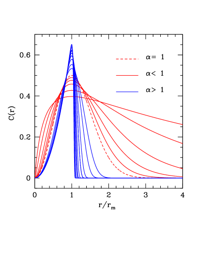
Figure 1: The left had plot shows the behavior of the compaction function varying the shape parameter $\alpha$ while the right panel shows the numerical data for $\delta_{c}$, using a blue line, in terms of $\alpha$ while the analytic fit given by (52) is plotted with a dashed line. In particular we are using here the curvature profile given by (50) for $\lambda=0$.

VI.1 The shape parameter

As seen in Musco (2019); Escrivà et al. (2020); Musco et al. (2021) the threshold for PBHs depends on the shape of the cosmological perturbation, characterized by the width of the peak of the compaction function $\mathcal{C}(r)$ defined in Eq. (21), measured by a dimensionless parameter $\alpha$ defined as

$$\alpha\equiv-\frac{r^{2}_{\mathrm{m}}\mathcal{C}^{\prime\prime}(r_{\mathrm{m}})}{4\mathcal{C}(r_{\mathrm{m}})}.$$ (43)

The radius $r_{\mathrm{m}}$ is the characteristic comoving scale of the perturbation, identified where the compaction function has a peak, corresponding to the the location where the gravitational filed reaches its maximum. The apparent horizon of a black hole forms in this region during the collapse if the height of the peak, measuring the perturbation amplitude $\delta$, is larger than a threshold $\delta_{\mathrm{c}}$.

For larger values of $\alpha$ the peak of the compaction function becomes sharper while the peak of the energy density perturbation gets broader, whereas for smaller values of $\alpha$ we have the opposite behavior. The strict relation between the shape of the compaction function and the shape of the energy density perturbation is related to the Birkhoff theorem, where the collapse is mainly affected by the matter distribution inside the region forming the black hole, characterized just by one parameter, plus very small second order corrections induced by the shape of the perturbation outside this region Musco (2019).

Looking at the quasi homogeneous solution derived in Sec. V we have

$$\mathcal{C}(r)\simeq\frac{r^{2}}{r^{2}_{\mathrm{m}}}\tilde{M}+O(\epsilon^{2})=\frac{2}{3}\mathcal{K}(r)r^{2}$$ (44)

which is a generalization of the expression for the isotropic solution, replacing $K(r)$ with $\mathcal{K}(r)$. The value of $r_{\mathrm{m}}$ is computed imposing $\mathcal{C}^{\prime}(r_{\mathrm{m}})=0$, which gives

$$\mathcal{K}(r_{\mathrm{m}})+\frac{r_{\mathrm{m}}}{2}\mathcal{K}^{\prime}(r_{\mathrm{m}})=0.$$ (45)

Using Eq. (38), we can explicitly write Eq. (45) as

$$K(r_{\mathrm{m}})+\frac{r_{\mathrm{m}}}{2}K^{\prime}(r_{\mathrm{m}})=\frac{\lambda}{r^{2}_{\mathrm{m}}}\Phi(a)\left[\mathcal{F}(r_{\mathrm{m}})+\frac{r_{\mathrm{m}}}{2}\mathcal{F}^{\prime}(r_{\mathrm{m}})\right].$$ (46)

To calculate the shape parameter $\alpha$ we insert Eq. (38) into Eq. (44) and calculate the second derivative $\mathcal{C}^{\prime\prime}(r_{\mathrm{m}})$. The full expression for $\alpha$ in terms of $K(r)$, $\mathcal{F}(r)$, $\Phi(a)$, $\lambda$ and $j$ is very complicated, but we can understand the qualitative effect of the anisotropy by making a perturbative expansion for $\lambda\ll 1$

$$\begin{split}\alpha\simeq\alpha_{0}\left\{1+\left[p(r_{\mathrm{m}})-q(r_{\mathrm{m}})\right]\Phi(a)\lambda\right.\\ \left.+p(r_{\mathrm{m}})q(r_{\mathrm{m}})\Phi^{2}(a)\lambda^{2}\right\},\end{split}$$ (47)

where $\alpha_{0}$ is the shape parameter when $\lambda=0$, and $p(r)$ and $q(r)$ are two dimensionless functions defined as

$$p(r) \equiv \frac{\mathcal{F}(r)}{K(r)r^{2}}$$ (48)

$$q(r) \equiv \frac{1}{r^{2}}\frac{\mathcal{F}^{\prime\prime}(r)r^{2}+4r\mathcal{F}^{\prime}(r)+2\mathcal{F}(r)}{K^{\prime\prime}(r)r^{2}+4rK^{\prime}(r)+2K(r)}.$$ (49)

The shape parameter $\alpha_{0}$ of the isotropic solution is related to a family of curvature profiles $K(r)$

$$K(r)=\mathcal{A}\exp\left[-\frac{1}{\alpha_{0}}\left(\frac{r}{r_{\mathrm{m,0}}}\right)^{2\alpha_{0}}\right],$$ (50)

where $r_{\mathrm{m,0}}$ is the comoving scale of the perturbation, obtained from Eq. (46) when $\lambda=0$, and $\mathcal{A}$ is a parameter varying the perturbation amplitude $\delta$ as (see Musco (2019) for more details)

$$\delta=\frac{2}{3}e^{-1/\alpha_{0}}\mathcal{A}\,r^{2}_{\mathrm{m,0}}\,.$$ (51)

The left plot of Figure 1 shows the compaction function profiles, obtained from (50) when $\lambda=0$, for different value of $\alpha$. The peak of the compaction function becomes broader (red lines) for smaller values of $\alpha$, corresponding to a shape of the energy density profiles more and more peaked. Instead for larger values of $\alpha$ the compaction function is more peaked (blue lines) while the energy density profiles become broader. For $\alpha=1$ we have the particular case of a Mexican hat shape for the energy density, obtained using a Gaussian profile for the curvature profile $K(r)$.

VI.2 The threshold for PBH formation

As the numerical simulations have shown, in a radiation dominated Universe there is a simple analytic relation for the threshold of PBH formation as a function of the shape parameter, $\alpha$, corresponding to the numerical fit given by Eq. (44) of Musco et al. (2021):

$$\delta_{\mathrm{c}}=\begin{cases}\alpha^{0.047}-0.50\quad\quad\quad 0.1\lesssim\alpha\lesssim 7\\ \alpha^{0.035}-0.475\quad\quad\quad 7\lesssim\alpha\lesssim 13\\ \alpha^{0.026}-0.45\quad\quad\quad 13\lesssim\alpha\lesssim 30.\end{cases}$$ (52)

This is represented in the right plot of Figure 1, where the numerical data is plotted with a blue line, while the fit given by (52) is plotted with a dashed line.

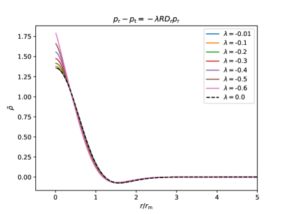
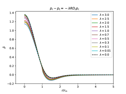
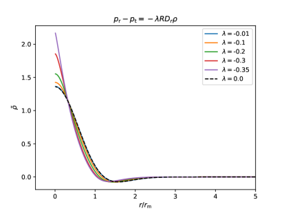
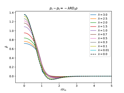
Figure 2: In this figure, we show the behavior of $\tilde{\rho}$ plotted against $r/r_{\mathrm{m}}$ for the special case $n=0$ from the family of models with $g(r,t)=R(r,t)$. In the top panels, we consider the case where the equation of state of the anisotropic fluid is given in terms of pressure gradients, following Eq. (13), whereas in the bottom panels we account for the case where the equation of state is given in terms of energy density gradients, following Eq. (14). The left panels consider negative values of the anisotropy parameter $\lambda$ while the right ones account for positive values.

Inserting (50) into Eq. (38), and solving numerically for the function $\mathcal{F}(r)$ (see Appendix B) to compute the profiles of the pressure or energy density gradients, we can study how the Mexican hat profile of the energy density, taken as a typical perturbation, is modified by the anisotropy, varying $\lambda$. To do this we consider a constant value of the perturbation amplitude $\delta=0.5$, taking into account that $\delta_{\mathrm{c}}\simeq 0.5$ is the threshold for the Mexican hat shape ($\alpha_{0}=1$ and $\lambda=0$). The relation between $\delta_{\mathrm{c}}$ and $\alpha$ given in (52) then allows the corresponding value of the threshold to be computed in terms of $\lambda$.

Here we are assuming that the effect of the anisotropy could be computed with the non linear modification of the shape, without modifying the relation between the shape and the threshold. This is a reasonable approximation without performing full non linear simulations of the anisotropic collapse.

After normalizing $r^{2}_{\mathrm{m,0}}=1$ and inserting this into Eq. (46) we find that $r_{\mathrm{m}}\simeq r_{\mathrm{m,0}}$ which means that there is no a significant change in the characteristic scale because of the anisotropy. The main effect on the shape is given by the competition of the two functions $p(r)$ and $q(r)$ defined in Eqs. (48) and (49). In general we have observed that $p(r_{\mathrm{m}})>q(r_{\mathrm{m}})$ and therefore from Eq. (47) one can easily infer that, considering terms up to order $O(\lambda)$ in Eq. (47), for positive values of $\lambda$ the value of the shape parameter $\alpha$ increases, making the shape of the compaction function sharper while the shape of the energy density perturbation profile becomes broader. On the other hand, negative values of $\lambda$ give a smaller value of $\alpha$, broadening the shape of the compaction function while the energy density perturbation profile gets steeper.

This behavior is shown explicitly in Figure 2, where we plot $\tilde{\rho}$ for different values of $\lambda$ when $g(r,t)=R(r,t)$: the upper plots correspond to the EoS expressed in terms of pressure gradients ($j=0$) while the bottom ones refer to the EoS expressed in terms of energy density gradients ($j=1$). The left plots of this figure are characterized by negative values of $\lambda$ while the right plots are characterized by positive values of $\lambda$.

Starting from $\lambda=0$ when the fluid is isotropic, we observe for $\lambda<0$ an increase of the amplitude of the peak of the energy density perturbation and the central profile sharpens more and more, consistently with the increase of the pressure gradients in the center observed in the left panels of Figure 2. This translates into a broadening of the peak of the compaction function, decreasing the value of $\delta_{\mathrm{c}}$ and enhancing in this way the formation of PBHs.

This could be explained with simple physical arguments by the following reasoning: given the fact that the pressure/energy density gradient profile is mainly negative (see Appendix B), from $p_{\mathrm{r}}-p_{\mathrm{t}}=-\lambda RD_{\mathrm{r}}\left(p_{\mathrm{r}}\rm{\;or\;}\rho\right)$, one has that $p_{\mathrm{r}}<p_{\mathrm{t}}$ and the radial pressure is reduced with respect to the tangential one. Because of this, one would expect it to be easier for a cosmological perturbation to collapse along the radial direction with respect to the isotropic case and consequently the peak of the energy density perturbation to be larger compared to the isotropic case with $\lambda=0$.

On the other hand, when $\lambda>0$ we have $p_{\mathrm{r}}>p_{\mathrm{t}}$, giving a larger value of the radial component of the pressure compared to the isotropic case. In this case the pressure gradients are increased around $r_{\mathrm{m}}$ as shown in the right panels of Figure 2. This translates into a reduced amplitude of the peak of the energy density perturbations with respect to the isotropic case, which makes the collapse of cosmological perturbations into PBHs more difficult, increasing consequently the value of $\delta_{\mathrm{c}}$.

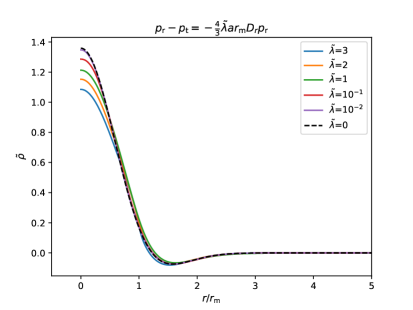
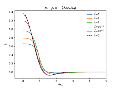
Figure 3: In this figure, we show the behavior of $\tilde{\rho}$ against $r/r_{\mathrm{m}}$ when $g(r,t)=\rho^{n}(r,t)$. In the left panel, we consider the case where the equation of state of the anisotropic fluid is given in terms of pressure gradients, following Eq. (15), whereas in the right panel we account for the case where the equation of state is given in terms of energy density gradients, following Eq. (16).

In Figure 3, we analyze the effect of the anisotropy on the profile of the energy density perturbation when the equation of state is characterized by $g(r,t)=\rho^{n}(r,t)$, rescaling the anisotropic parameter, measured at horizon crossing $a_{\mathrm{HC}}$, in a dimensionless form

$$\tilde{\lambda}\equiv\lambda\Phi(a_{\mathrm{HC}}),$$ (53)

which allows he EoS to be rewritten as

$$p_{\mathrm{r}}=\frac{1}{3}\left[\rho-2\tilde{\lambda}r_{\mathrm{m}}\chi_{n}(a)\left(\frac{\rho}{\rho_{\mathrm{b,i}}}\right)^{n}D_{\mathrm{r}}\left\{\begin{split}&p_{\mathrm{r}}&(j=0)\\ &\rho&(j=1)\end{split}\right\}\right],$$ (54)

where

$$\chi_{n}(a)\equiv\frac{2a_{\mathrm{i}}(1-2n)}{3}\frac{\displaystyle{\left(\frac{a}{a_{\mathrm{i}}}\right)^{3}}}{\left[\displaystyle{\left(\frac{a}{a_{\mathrm{i}}}\right)^{2(1-2n)}-1}\right]}\,.$$ (55)

In this case, we consider only positive values of $\tilde{\lambda}$ because of the structure of the equations for the pressure or energy density gradients (see Eq. (65) and (66) in Appendix B.2).

As we have discussed in Section V.2, this EoS introduces a characteristic scale into the problem, which requires specification of an additional parameter $\mu\equiv\left(\frac{\rho_{\mathrm{b,HC}}}{\rho_{\mathrm{b,i}}}\right)^{1/4}$  , defined as the ratio between the energy scales at horizon crossing ($\epsilon_{\mathrm{HC}}=1$) and at the initial time $t_{i}$, when the perturbations are generated. This time depends on the particular cosmological model of the early Universe being considered (e.g. inflation).

From the EoS seen in Eq. (54) one can identify three main contributions: the dimensionless parameter $\tilde{\lambda}$ accounting for the anisotropy of the medium, the term $\left(\frac{\rho}{\rho_{\mathrm{b,i}}}\right)^{n}$ measuring the effect of cosmic expansion, and finally $D_{\mathrm{r}}\left(p_{\mathrm{r}}\rm\ \textrm{or}\ \rho\right)$ which accounts for the effect of the pressure or energy density gradients. As it seems reasonable, we assume that for $t\to\infty$ the contribution of the pressure and energy density gradients disappears. This constrains the value of the exponent of $\rho$ just to non negative values ($n\geq 0$) and it is interesting to note that this is discarding the solution analyzed in Sec. V.1.

In Figure 3 we analyze the simplest model with $n=0$ and $\mu=10^{-10}$. The qualitative behavior is similar to the case where $g(r,t)=R(r,t)$ with a positive value of $\tilde{\lambda}$ enhancing the radial pressure compared to the tangential one and reducing the height of the peak of $\tilde{\rho}$ with respect the isotropic case, making in this way more difficult for cosmological perturbations to collapse into PBHs. This is confirmed by the behavior of the pressure gradients seen in Fig. 7, similar to the one seen in the right plots of Fig. 6.

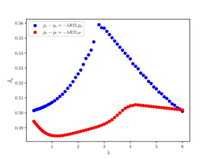
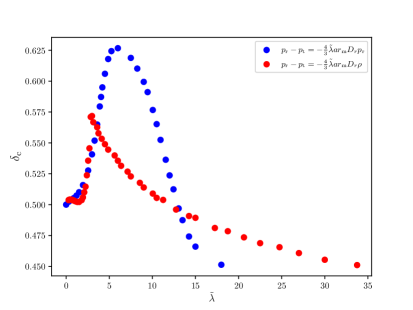
Figure 4: This figure shows the threshold of PBHs $\delta_{\mathrm{c}}$ as a function of the amplitude of the anisotropy in linear scale. In the left panel, we see the case where $g(r,t)=R(r,t)$ while in the right panel we consider a more general model with $g(r,t)=\rho^{n}(r,t)$. For both cases the blue dots indicate the values of the threshold when the anisotropic term of the equation of state is modeled in terms of pressure gradients while the red dots correspond to values of the threshold when the anisotropic term is written in terms of gradients of the energy density.

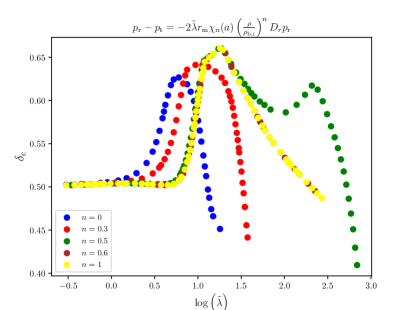
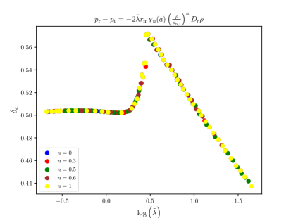
Figure 5: This figure shows the threshold of PBHs $\delta_{\mathrm{c}}$ as a function of the amplitude of the anisotropy using when the equation of state is characterized by $g(r,t)=\rho^{n}(r,t)$ for $n=0,0.3,0.5,0.6,1$. In the left panel we see the case of the equation of state having an implicit form when this expressed in terms of pressure gradients, while in the right panel this has an explicit form as it is expressed in terms of density gradients.

The effect of the anisotropy on the shape of the energy density perturbation can be used to estimate the corresponding effect on the threshold $\delta_{\mathrm{c}}$ for PBH formation. To do so, we make the assumption that $\delta_{\mathrm{c}}$ has the same dependence on the shape of the initial energy density perturbation profile seen in the isotropic case, as given by (52). This enables us to study how $\delta_{\mathrm{c}}$ is varying with respect to the amplitude of the anisotropy, as shown explicitly in Fig. 4, both for the model plotted in Fig. 2 when $g(r,t)=R(r,t)$ (left panel) and for the model of Fig. 3, when $g(r,t)=\rho^{n}(r,t)$, using in particular $n=0$ and $\mu=10^{-10}$ (right panel). Finally in Fig. 5 we study the behavior of $\delta_{c}$ when $g(r,t)=\rho^{n}(r,t)$ for different values of $n$, considering in the left panel the EoS written in terms of pressure gradients while in the right one the EoS written in terms of density gradients is used.

In general we observe an initial increase of $\delta_{\mathrm{c}}$ with respect to $\lambda$ or $\tilde{\lambda}$, which is somehow expected, as already explained, because the shape parameter $\alpha$ becomes larger for an increasing amplitude of the anisotropy, enhancing the radial pressure with respect to the tangential one. However from these figure we can see a critical value of $\lambda$ and $\tilde{\lambda}$, followed by a decreasing behavior of $\delta_{\mathrm{c}}$, when the modification of the shape parameter due to the anisotropy is non linear. This effect is due to the term $O(\lambda^{2})$ in Eq. (47), becoming important when $\lambda\sim 1$. Obviously this regime is challenging the validity of our approximation of computing the threshold using the isotropic relation between $\delta_{c}$ and $\alpha$, and this result should therefore be considered with care.

Fig. 5 shows that, while the model in terms of pressure gradients has a different behavior for different values of $n$, the model of the EoS written in terms of density gradients shows a universal behavior, independent of the particular value of $n$. This difference can be explained by the implicit solution of the equation of state, when this is expressed in terms of the pressure gradients with respect to the explicit form which has when written in terms of the density gradients.

Although these results are genuinely interesting and find a clear physical explanation, we stress again that one cannot fully trust the perturbative approach in the regime where $\delta_{\mathrm{c}}$ is decreasing and full numerical simulations solving the non-linear hydrodynamic equations are necessary to confirm to which extent Eq. (52) holds for a non linear amplitude of the anisotropy.

Despite this, the results obtained here give a reasonable estimation of the effect of the anisotropy on the threshold of PBH formation when the anisotropy is not too large, with a change of the threshold up to $25\%$. This would mean, potentially, a relevant change of the abundance for PBHs if the early Universe was significantly non isotropic.

VII Conclusions

In this work, we have studied the formation of PBHs within a radiation fluid described by an anisotropic pressure. By making use of a covariant formulation of the equation of state and performing a gradient expansion approximation on superhorizon scales we have computed the anisotropic quasi homogeneous solution describing the initial conditions that one would need to use in the future for numerical simulations. Using this solution we have investigated the effect of the anisotropy on the shape of the energy density perturbation profile, estimating the corresponding value of the threshold for PBHs, assuming that $\delta_{\mathrm{c}}$ has the same behavior with the shape of the energy density profile as when the fluid is isotropic.

Although the estimation of the threshold for PBH computed here is consistent only for small values of the anisotropy parameter ($\lambda\ll 1$), the qualitative behavior found for $\delta_{\mathrm{c}}$ looks to be consistent, and gives a reasonable solution to a problem that has never been studied before. To obtain a more quantitative and precise answer to such a problem, when the amplitude of the anisotropy is not small, it would be necessary to perform full numerical simulations, generalizing for example the code used in previous works of this type, as in Musco et al. (2005); Polnarev and Musco (2007); Musco et al. (2009); Musco and Miller (2013); Musco (2019); Musco et al. (2021).

Before concluding we should comment here on the model with $g(r,r)=R(r,t)$ where the behavior of $\alpha$ and $\delta_{\mathrm{c}}$ is significantly different when $p_{\mathrm{r}}-p_{\mathrm{t}}$ is proportional to the pressure gradients from the case when it is proportional to the energy density gradients. In the first case $\delta_{\mathrm{c}}$ is initially increasing with $\lambda$ up to a critical point and then decreases, while in the second case $\delta_{\mathrm{c}}$ is first decreasing and then increasing. It is difficult to understand the physical motivation of this discordant behavior. This model however is not based on solid physical grounds, because the EoS with $g(r,t)=R(r,t)$ is not expressed in terms of local quantities, as one would normally expect. This is a special case of the model described in Sec. V.2, with $n=-1/4$, where the pressure or energy density gradients do not vanish for an infinite expansion, as one would expect.

Analyzing this first model has been useful to simplify the problem, understanding how to write the anisotropic quasi homogeneous solution in a clear and self consistent form. However, only the model elaborated later in Sec. V.2, where the EoS is written only in terms of local quantities, and the anisotropy is varying also with the expansion of the Universe, looks to be physically plausible, and therefore should be seriously taken into account for further studies on the subject, with particular attention to the version where the EoS is written in terms of density gradients, characterized by an explicit solution.

Appendix A EoS with $g(r,t)=\rho^{n}(r,t)$ and $n=1/2,1/4$

Here we discuss the particular cases when $n=1/2$ and $n=1/4$. Looking at Eq. (41), one can see that the functions $\Phi$ , $I_{1}$ and $I_{2}$ diverge due to the prefactor $1/(1-2n)$ in $\Phi$ and $1/\left[(1-2n)(1-4n)\right]$ in $I_{1}$ and $I_{2}$. However, computing carefully these limits for $n\to 1/2$ one gets

$$\Phi(a) =\frac{3\sqrt{\rho_{\mathrm{b,i}}}}{a_{\mathrm{i}}r_{\mathrm{m}}}\left(\frac{a}{a_{\mathrm{i}}}\right)^{-3}\ln\left(\frac{a}{a_{\mathrm{i}}}\right)$$ (56)

$$I_{1}(a) =\frac{\sqrt{\rho_{\mathrm{b,i}}}}{2a_{\mathrm{i}}r_{\mathrm{m}}}\left(\frac{a}{a_{\mathrm{i}}}\right)^{-3}\left[2-2\frac{a}{a_{\mathrm{i}}}+\ln\left(\frac{a}{a_{\mathrm{i}}}\right)\right]$$ (57)

$$I_{2}(a) =\frac{\sqrt{\rho_{\mathrm{b,i}}}}{a_{\mathrm{i}}r_{\mathrm{m}}}\left(\frac{a}{a_{\mathrm{i}}}\right)^{-3}\left[\ln\left(\frac{a}{a_{\mathrm{i}}}\right)-\frac{a}{a_{\mathrm{i}}}+1\right]\ \,,$$ (58)

while for $n\to 1/4$ one has

$$I_{1}(a) =\frac{\rho^{1/4}_{\mathrm{b,i}}}{2a_{\mathrm{i}}r_{\mathrm{m}}}\left(\frac{a}{a_{\mathrm{i}}}\right)^{-3}\left\{\frac{a}{a_{\mathrm{i}}}\left[1-2\ln\left(\frac{a}{a_{\mathrm{i}}}\right)\right]-1\right\}$$ (59)

$$I_{2}(a) =\frac{\rho^{1/4}_{\mathrm{b,i}}}{a_{\mathrm{i}}r_{\mathrm{m}}}\left(\frac{a}{a_{\mathrm{i}}}\right)^{-3}\left\{\frac{a}{a_{\mathrm{i}}}\left[1-\ln\left(\frac{a}{a_{\mathrm{i}}}\right)\right]-1\right\}\,.$$ (60)

Appendix B Density and pressure gradients

In this appendix, we give some additional details concerning the pressure and energy density gradient profiles for both EoSs, $g(r,t)=R(r,t)$ and $g(r,t)=\rho^{n}(r,t)$.

B.1 Equation of state with $g(r,t)=R(r,t)$

In the case where the equation of state is given in terms of pressure gradients, following Eq. (13), in order to get $\frac{\partial\tilde{p}_{\mathrm{r}}}{\partial r}$, one should combine Eq. (25) and the equation for $\tilde{\rho}$ from Eq. (28) to find the behavior of $f(r)$ defined in Eq. (27) as solution of the following differential equation:

$$\frac{4\lambda}{3}r\sqrt{1-K(r)r^{2}}f^{\prime}(r)+\left[\frac{7\lambda}{3}\sqrt{1-K(r)r^{2}}+\frac{3}{2}\right]f(r)$$ (61)

$$-\left\{\frac{\left[r^{3}K(r)\right]^{\prime}}{3r^{2}}\right\}^{\prime}r^{2}_{\mathrm{m}}\sqrt{1-K(r)r^{2}}=0,$$

with the boundary condition $f(0)=0$, as imposed by Eq. (12). For $\lambda=0$ one recovers the isotropic quasi-homogeneous limit,

$$f_{\lambda=0}(r)=\frac{2}{3}\left\{\frac{\left[r^{3}K(r)\right]^{\prime}}{3r^{2}}\right\}^{\prime}r^{2}_{\mathrm{m}}\sqrt{1-K(r)r^{2}}.$$ (62)

Solving Eq. (61) for $f(r)$, which allows to compute explicitly $\mathcal{F}(r)$ in Eq. (30), one obtains the explicit for of the quasi homogeneous solution given in (28) written in terms of a given curvature profile $K(r)$.

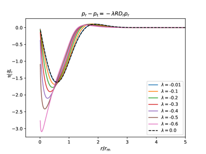
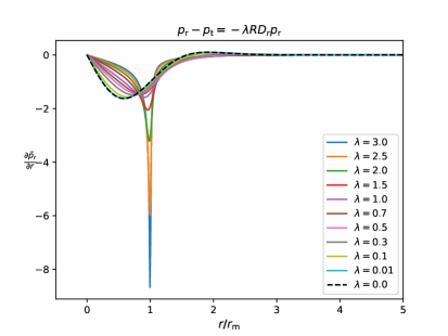
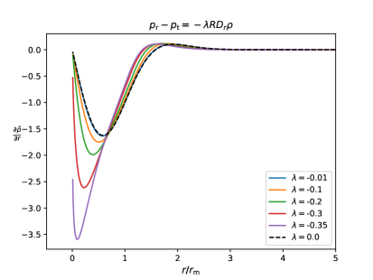
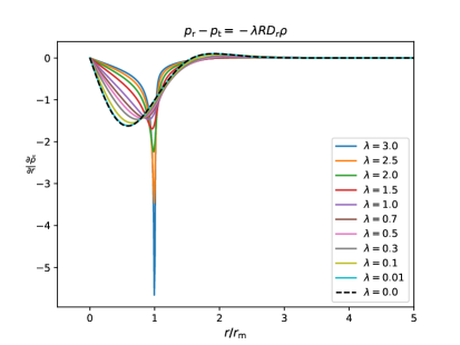
Figure 6: In this figure, we show the behavior of $\frac{\partial\tilde{p}_{\mathrm{r}}}{\partial r}$ and $\frac{\partial\tilde{\rho}}{\partial r}$ plotted against $r/r_{\mathrm{m}}$. The top panels concern the case where the equation of state is given in terms of pressure gradients, following Eq. (13), whereas the bottom panels are for the case where the equation of state is given in terms of energy density gradients, following Eq. (14). The left figures show the gradient profiles when $\lambda<0$ whereas the right ones consider values of $\lambda>0$.

In the case where the equation of state is given in terms of energy density gradients, following Eq. (14), with the same reasoning as before one gets the following equation for $f(r)$:

$$\frac{2\lambda}{3}r\sqrt{1-K(r)r^{2}}f^{\prime}(r)+\left[\frac{8\lambda}{3}\sqrt{1-K(r)r^{2}}+1\right]f(r)+$$ (63)

$$-2\left\{\frac{\left[r^{3}K(r)\right]^{\prime}}{3r^{2}}\right\}^{\prime}r^{2}_{\mathrm{m}}\sqrt{1-K(r)r^{2}}=0,$$

with the boundary condition $f(0)=0$.

In Figure 6, we show the pressure and energy density gradient profiles for positive and negative values of the anisotropy parameter $\lambda$. As one can clearly see, in the case where $\lambda<0$, there is a divergence of the pressure and energy density gradient profile in the center below a critical value. This behavior is due to the mathematical structure of Eq. (61) and Eq. (63), where the radial derivatives of $\tilde{p}_{\mathrm{r}}$ and $\tilde{\rho}$ diverge at $r=0$, for $\lambda<-9/14$ and $\lambda<-3/8$, respectively.

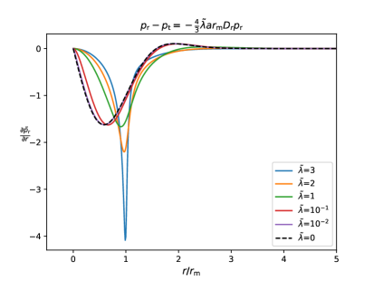
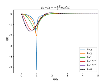
Figure 7: In this figure we show the behavior of $\frac{\partial\tilde{p}_{\mathrm{r}}}{\partial r}$ (left panel) and $\frac{\partial\tilde{\rho}}{\partial r}$ (right panel) potted against $r/r_{\mathrm{m}}$ for $n=0$ and $\lambda>0$.

To see this more in detail, consider for example the EoS in terms of the pressure gradients (the same applies also for the energy density gradients) and develop $f(r)$ defined in Eq. (27) around zero as

$$f(r)=j_{0}+j_{1}r+j_{2}r^{2}/2,$$

where

$$j_{0}=f(0)=\tilde{p}^{\prime}_{\mathrm{r}}(0)\,,\quad j_{1}=f^{\prime}(0)\quad\textrm{and}\quad j_{2}=f^{\prime\prime}(0)$$

and then using the differential equation (61) we get that

$$\frac{8\lambda r}{9}\left(1-\frac{\mathcal{A}r^{2}}{2}\right)\left(j_{0}+j_{1}r\right)$$ (64)

$$+\left[\frac{14\lambda}{9}\left(1-\frac{\mathcal{A}r^{2}}{2}\right)+1\right]\left(j_{0}+j_{1}r+\frac{j_{2}r^{2}}{2}\right)$$

$$-\tilde{p}^{\prime}_{\mathrm{r,iso}}\left(1-\frac{\mathcal{A}r^{2}}{2}\right)=0\,.$$

Taking now the limit as $r\to 0$ we obtain that

$$j_{0}=\tilde{p}^{\prime}_{\mathrm{r}}(0)=\lim_{r\to 0}\frac{\tilde{p}^{\prime}_{\mathrm{r,iso}}(r)}{1+\frac{14\lambda}{9}},$$

where $\tilde{p}^{\prime}_{\mathrm{r,iso}}=\frac{2}{3}\left\{\frac{\left[r^{3}K(r)\right]^{\prime}}{3r^{2}}\right\}^{\prime}r^{2}_{\mathrm{m}}$.

If $\lambda<-9/14$ one gets that $\tilde{p}^{\prime}_{\mathrm{r}}(0)=0^{+}$ which is not consistent because $\tilde{p}^{\prime}_{\mathrm{r}}(0)$ should approach zero from negative values, namely $\tilde{p}^{\prime}_{\mathrm{r,iso}}(0)=0^{-}$. However, if $\lambda>-9/14$ one obtains the consistent result that $\tilde{p}^{\prime}_{\mathrm{r}}(0)=0^{-}$. For the critical value $\lambda=-9/14$, applying the De l’Hopital theorem and considering that $\tilde{p}^{\prime\prime}_{\mathrm{r,iso}}(0)<0$, one gets

$$\tilde{p}^{\prime}_{\mathrm{r}}(0)=\lim_{r\to 0}\frac{\tilde{p}^{\prime}_{\mathrm{r,iso}}(r)}{1+\frac{14\lambda}{9}}=-\infty\neq 0^{-}\,.$$

In the case of $p_{\mathrm{r}}-p_{\mathrm{t}}=-\lambda RD_{\mathrm{r}}p_{\mathrm{r}}$ with $\lambda<0$ one gets that $\lambda$ should be larger than a critical value, namely $\lambda>\lambda_{\mathrm{c}}=-9/14$. When $p_{\mathrm{r}}-p_{\mathrm{t}}=-\lambda RD_{\mathrm{r}}\rho$, following the same procedure, one obtains that $\lambda>\lambda_{\mathrm{c}}=-3/8$ in order to avoid $\frac{\partial\tilde{\rho}}{\partial r}$ diverging at $r=0$.

B.2 Equation of state with $g(r,t)=\rho^{n}(r,t)$

In the case where the EoS is given in terms of pressure gradients, following Eq. (15), one should combine Eq. (34) and $\tilde{\rho}$ from Eq. (37) to obtain after a straightforward calculation the following differential equation for the function $f(r)$:

$$\begin{aligned} &\sqrt{1-K(r)r^{2}}\left[\frac{\rho^{n}_{\mathrm{b}}(a)}{\rho^{n}_{\mathrm{b,i}}}\frac{\chi_{n}(a)}{a}+\frac{1}{3}\right]\tilde{\lambda}rf^{\prime}(r)\\ &+\left\{\left[\frac{\rho^{n}_{\mathrm{b}}(a)}{\rho^{n}_{\mathrm{b,i}}}\frac{\chi_{n}(a)}{a}+\frac{4}{3}\right]\tilde{\lambda}\sqrt{1-K(r)r^{2}}+\frac{3r}{2r_{\mathrm{m}}}\right\}f(r)\\ &-\left[\frac{\left(r^{3}K(r)\right)^{\prime}}{3r^{2}}\right]^{\prime}r_{\mathrm{m}}\sqrt{1-K(r)r^{2}}=0\end{aligned},$$ (65)

where $f(r)$ is defined in Eq. (36) . The above differential equation should satisfy the boundary condition $\lim_{r\rightarrow 0}f(r)=0$ as imposed by Eq. (12).

Finally, in the case where the equation of state is given in terms of energy density gradients, following Eq. (16), with the same reasoning as before one obtains the following differential equation for the function $f(r)$:

$$\begin{aligned} &\frac{2\tilde{\lambda}\sqrt{1-K(r)r^{2}}}{3}rf^{\prime}(r)\\ &+\left\{\frac{8\tilde{\lambda}}{3}\sqrt{1-K(r)r^{2}}+\frac{r}{r_{\mathrm{m}}}\right\}f(r)\\ &-2\left[\frac{\left(r^{3}K(r)\right)^{\prime}}{3r^{2}}\right]^{\prime}r_{\mathrm{m}}\sqrt{1-K(r)r^{2}}=0\end{aligned},$$ (66)

with $\lim_{r\rightarrow 0}f(r)=0$.

In Figure 7 we show the pressure and energy density gradient profiles for different values of $\lambda$ and $n=0$. In this case, negative values of $\lambda$ lead to a divergence of the radial derivatives of $\tilde{p}_{\mathrm{r}}$ and $\tilde{\rho}$ at $r=0$ and therefore they should not be taken into account. This can be seen by applying the same gradient expansion around zero for Eq. (65) as before, which gives

$$\tilde{p_{\mathrm{r}}}^{\prime}(0)=\lim_{r\to 0}\frac{\tilde{p}^{\prime}_{\mathrm{r,iso}}(r)}{\frac{2}{3(1-2n)}\frac{\lambda\rho^{n}_{\mathrm{b,i}}}{\mu}\left(\frac{\mu}{\epsilon}\right)^{3}\left[(3-2n)\left(\frac{\mu}{\epsilon}\right)^{4n-2}-2\right]},$$

where $\tilde{p}^{\prime}_{\mathrm{r,iso}}=\frac{2}{3}\left\{\frac{\left[r^{3}K(r)\right]^{\prime}}{3r^{2}}\right\}^{\prime}r^{2}_{\mathrm{m}}$, and the necessary condition in order not to have a divergence at $r=0$ is

$$\frac{3}{2(1-2n)}\frac{\lambda}{\mu}\left(\frac{\mu}{\epsilon}\right)^{3}\left[(3-2n)\left(\frac{\mu}{\epsilon}\right)^{4n-2}-2\right]>0.$$ (67)

From the above expression, fixing $\mu$ and $\epsilon$ one may identify two regimes, $n>1/2$ and $n<1/2$. In particular, when $n>1/2$ assuming that $\mu/\epsilon\ll 1$, one obtains that the second term within the square brackets of Eq. (67) is dominant and $\lambda>0$. On the other hand, if $n<1/2$ the first term within the brackets is now dominating, and one again gets $\lambda>0$. Therefore, if $\mu/\epsilon\ll 1$ one has in general that $\lambda>\lambda_{\mathrm{c}}=0$.

Finally, when the difference between the radial and the tangential pressure is proportional to the energy density gradients, by following the same reasoning, one gets the following necessary condition to avoid divergences around $r=0$

$$\frac{4}{1-2n}\frac{\lambda}{\mu}\left(\frac{\mu}{\epsilon}\right)^{3}\left[1-\left(\frac{\mu}{\epsilon}\right)^{4n-2}\right]<0\,,$$ (68)

and if $\mu/\epsilon_{0}\ll 1$, we again have $\lambda>0$ for any value of $n$.

References

- Zel’dovich (1967) Y. B. . N. Zel’dovich, I. D., Soviet Astron. AJ (Engl. Transl. ), 10, 602 (1967).
- Hawking (1971) S. Hawking, Mon. Not. Roy. Astron. Soc. 152, 75 (1971).
- Carr and Hawking (1974) B. J. Carr and S. W. Hawking, Mon. Not. Roy. Astron. Soc. 168, 399 (1974).
- Sasaki et al. (2018) M. Sasaki, T. Suyama, T. Tanaka, and S. Yokoyama, Class. Quant. Grav. 35, 063001 (2018), arXiv:1801.05235 [astro-ph.CO] .
- Green and Kavanagh (2021) A. M. Green and B. J. Kavanagh, J. Phys. G 48, 043001 (2021), arXiv:2007.10722 [astro-ph.CO] .
- Carr et al. (2020) B. Carr, K. Kohri, Y. Sendouda, and J. Yokoyama, (2020), arXiv:2002.12778 [astro-ph.CO] .
- Abbott et al. (2019) B. Abbott et al. (LIGO Scientific, Virgo), Phys. Rev. X 9, 031040 (2019), arXiv:1811.12907 [astro-ph.HE] .
- Abbott et al. (2020a) R. Abbott et al. (LIGO Scientific, Virgo), Phys. Rev. D 102, 043015 (2020a), arXiv:2004.08342 [astro-ph.HE] .
- Abbott et al. (2020b) R. Abbott et al. (LIGO Scientific, Virgo), Astrophys. J. Lett. 896, L44 (2020b), arXiv:2006.12611 [astro-ph.HE] .
- Abbott et al. (2020c) R. Abbott et al. (LIGO Scientific, Virgo), Phys. Rev. Lett. 125, 101102 (2020c), arXiv:2009.01075 [gr-qc] .
- Sasaki et al. (2016) M. Sasaki, T. Suyama, T. Tanaka, and S. Yokoyama, Phys. Rev. Lett. 117, 061101 (2016), [erratum: Phys. Rev. Lett.121,no.5,059901(2018)], arXiv:1603.08338 [astro-ph.CO] .
- Bird et al. (2016) S. Bird, I. Cholis, J. B. Muñoz, Y. Ali-Haïmoud, M. Kamionkowski, E. D. Kovetz, A. Raccanelli, and A. G. Riess, Phys. Rev. Lett. 116, 201301 (2016), arXiv:1603.00464 [astro-ph.CO] .
- Clesse and García-Bellido (2017) S. Clesse and J. García-Bellido, Phys. Dark Univ. 15, 142 (2017), arXiv:1603.05234 [astro-ph.CO] .
- Ali-Haïmoud et al. (2017) Y. Ali-Haïmoud, E. D. Kovetz, and M. Kamionkowski, Phys. Rev. D 96, 123523 (2017), arXiv:1709.06576 [astro-ph.CO] .
- Raidal et al. (2019) M. Raidal, C. Spethmann, V. Vaskonen, and H. Veermäe, JCAP 1902, 018 (2019), arXiv:1812.01930 [astro-ph.CO] .
- Hütsi et al. (2019) G. Hütsi, M. Raidal, and H. Veermäe, Phys. Rev. D 100, 083016 (2019), arXiv:1907.06533 [astro-ph.CO] .
- Vaskonen and Veermäe (2020) V. Vaskonen and H. Veermäe, Phys. Rev. D 101, 043015 (2020), arXiv:1908.09752 [astro-ph.CO] .
- Gow et al. (2020) A. D. Gow, C. T. Byrnes, A. Hall, and J. A. Peacock, JCAP 01, 031 (2020), arXiv:1911.12685 [astro-ph.CO] .
- De Luca et al. (2020a) V. De Luca, G. Franciolini, P. Pani, and A. Riotto, Phys. Rev. D 102, 043505 (2020a), arXiv:2003.12589 [astro-ph.CO] .
- De Luca et al. (2020b) V. De Luca, G. Franciolini, P. Pani, and A. Riotto, JCAP 06, 044 (2020b), arXiv:2005.05641 [astro-ph.CO] .
- Clesse and Garcia-Bellido (2020) S. Clesse and J. Garcia-Bellido, (2020), arXiv:2007.06481 [astro-ph.CO] .
- Hall et al. (2020) A. Hall, A. D. Gow, and C. T. Byrnes, Phys. Rev. D 102, 123524 (2020), arXiv:2008.13704 [astro-ph.CO] .
- Jedamzik (2020) K. Jedamzik, JCAP 09, 022 (2020), arXiv:2006.11172 [astro-ph.CO] .
- Jedamzik (2021) K. Jedamzik, Phys. Rev. Lett. 126, 051302 (2021), arXiv:2007.03565 [astro-ph.CO] .
- De Luca et al. (2021a) V. De Luca, V. Desjacques, G. Franciolini, P. Pani, and A. Riotto, Phys. Rev. Lett. 126, 051101 (2021a), arXiv:2009.01728 [astro-ph.CO] .
- De Luca et al. (2020c) V. De Luca, V. Desjacques, G. Franciolini, and A. Riotto, JCAP 11, 028 (2020c), arXiv:2009.04731 [astro-ph.CO] .
- Wong et al. (2021) K. W. K. Wong, G. Franciolini, V. De Luca, V. Baibhav, E. Berti, P. Pani, and A. Riotto, Phys. Rev. D 103, 023026 (2021), arXiv:2011.01865 [gr-qc] .
- Arzoumanian et al. (2020) Z. Arzoumanian et al. (NANOGrav), Astrophys. J. Lett. 905, L34 (2020), arXiv:2009.04496 [astro-ph.HE] .
- Vaskonen and Veermäe (2021) V. Vaskonen and H. Veermäe, Phys. Rev. Lett. 126, 051303 (2021), arXiv:2009.07832 [astro-ph.CO] .
- De Luca et al. (2021b) V. De Luca, G. Franciolini, and A. Riotto, Phys. Rev. Lett. 126, 041303 (2021b), arXiv:2009.08268 [astro-ph.CO] .
- Kohri and Terada (2021) K. Kohri and T. Terada, Phys. Lett. B 813, 136040 (2021), arXiv:2009.11853 [astro-ph.CO] .
- Domènech and Pi (2020) G. Domènech and S. Pi, (2020), arXiv:2010.03976 [astro-ph.CO] .
- Sugiyama et al. (2021) S. Sugiyama, V. Takhistov, E. Vitagliano, A. Kusenko, M. Sasaki, and M. Takada, Phys. Lett. B 814, 136097 (2021), arXiv:2010.02189 [astro-ph.CO] .
- Inomata et al. (2021) K. Inomata, M. Kawasaki, K. Mukaida, and T. T. Yanagida, Phys. Rev. Lett. 126, 131301 (2021), arXiv:2011.01270 [astro-ph.CO] .
- Nadezhin et al. (1978) D. K. Nadezhin, I. D. Novikov, and A. G. Polnarev, Soviet Astronomy 22, 129 (1978).
- Bicknell and Henriksen (1979) G. V. Bicknell and R. N. Henriksen, Astrophysics Journal 232, 670 (1979).
- Novikov and Polnarev (1979) I. D. Novikov and A. G. Polnarev, in Sources of Gravitational Radiation, edited by L. L. Smarr (1979) pp. 173–190.
- Jedamzik and Niemeyer (1999) K. Jedamzik and J. C. Niemeyer, Phys. Rev. D 59, 124014 (1999), arXiv:astro-ph/9901293 .
- Shibata and Sasaki (1999a) M. Shibata and M. Sasaki, Phys. Rev. D 60, 084002 (1999a), arXiv:gr-qc/9905064 .
- Hawke and Stewart (2002) I. Hawke and J. Stewart, Class. Quant. Grav. 19, 3687 (2002).
- Musco et al. (2005) I. Musco, J. C. Miller, and L. Rezzolla, Class. Quant. Grav. 22, 1405 (2005), arXiv:gr-qc/0412063 .
- Polnarev and Musco (2007) A. G. Polnarev and I. Musco, Class. Quant. Grav. 24, 1405 (2007), arXiv:gr-qc/0605122 .
- Musco et al. (2009) I. Musco, J. C. Miller, and A. G. Polnarev, Class. Quant. Grav. 26, 235001 (2009), arXiv:0811.1452 [gr-qc] .
- Musco and Miller (2013) I. Musco and J. C. Miller, Class. Quant. Grav. 30, 145009 (2013), arXiv:1201.2379 [gr-qc] .
- Harada et al. (2013) T. Harada, C.-M. Yoo, and K. Kohri, Phys. Rev. D88, 084051 (2013), [Erratum: Phys. Rev.D89,no.2,029903(2014)], arXiv:1309.4201 [astro-ph.CO] .
- Musco (2019) I. Musco, Phys. Rev. D 100, 123524 (2019), arXiv:1809.02127 [gr-qc] .
- Escrivà et al. (2020) A. Escrivà, C. Germani, and R. K. Sheth, Phys. Rev. D 101, 044022 (2020), arXiv:1907.13311 [gr-qc] .
- Musco et al. (2021) I. Musco, V. De Luca, G. Franciolini, and A. Riotto, Phys. Rev. D 103, 063538 (2021), arXiv:2011.03014 [astro-ph.CO] .
- Bardeen et al. (1986) J. M. Bardeen, J. Bond, N. Kaiser, and A. Szalay, Astrophys. J. 304, 15 (1986).
- Lin et al. (1965) C. C. Lin, L. Mestel, and F. H. Shu, Astrophysics Journal 142, 1431 (1965).
- Doroshkevich (1970) A. G. Doroshkevich, Astrophysics 6, 320 (1970).
- Zel’Dovich (1970) Y. B. Zel’Dovich, Astronomy and Astrophysics 500, 13 (1970).
- Khlopov and Polnarev (1980) M. Y. Khlopov and A. G. Polnarev, Physics Letters B 97, 383 (1980).
- Harada and Jhingan (2016) T. Harada and S. Jhingan, PTEP 2016, 093E04 (2016), arXiv:1512.08639 [gr-qc] .
- Kühnel and Sandstad (2016) F. Kühnel and M. Sandstad, Phys. Rev. D 94, 063514 (2016), arXiv:1602.04815 [astro-ph.CO] .
- Letelier (1982) P. S. Letelier, Nuovo Cimento B Serie 69, 145 (1982).
- Bowers and Liang (1974) R. L. Bowers and E. P. T. Liang, Astrophysics Journal 188, 657 (1974).
- Letelier (1980) P. S. Letelier, Physical Review D 22, 807 (1980).
- Bayin (1982) S. S. Bayin, Phys. Rev. D 26, 1262 (1982).
- Mak and Harko (2003) M. K. Mak and T. Harko, Proc. Roy. Soc. Lond. A 459, 393 (2003), arXiv:gr-qc/0110103 .
- Dev and Gleiser (2004) K. Dev and M. Gleiser, Int. J. Mod. Phys. D 13, 1389 (2004), arXiv:astro-ph/0401546 .
- Herrera et al. (2004) L. Herrera, A. Di Prisco, J. Martin, J. Ospino, N. O. Santos, and O. Troconis, Phys. Rev. D 69, 084026 (2004), arXiv:gr-qc/0403006 .
- Veneroni and da Silva (2018) L. S. M. Veneroni and M. F. A. da Silva, Int. J. Mod. Phys. D 28, 1950034 (2018), arXiv:1807.09926 [gr-qc] .
- Doneva and Yazadjiev (2012) D. D. Doneva and S. S. Yazadjiev, Phys. Rev. D 85, 124023 (2012), arXiv:1203.3963 [gr-qc] .
- Biswas and Bose (2019) B. Biswas and S. Bose, Phys. Rev. D 99, 104002 (2019), arXiv:1903.04956 [gr-qc] .
- Raposo et al. (2019) G. Raposo, P. Pani, M. Bezares, C. Palenzuela, and V. Cardoso, Phys. Rev. D99, 104072 (2019), arXiv:1811.07917 [gr-qc] .
- Misner and Sharp (1964) C. W. Misner and D. H. Sharp, Phys. Rev. 136, B571 (1964).
- Hayward (1996) S. A. Hayward, Phys. Rev. D 53, 1938 (1996), arXiv:gr-qc/9408002 .
- May and White (1966) M. M. May and R. H. White, Phys. Rev. 141, 1232 (1966).
- Bowers and Liang (1974) R. L. Bowers and E. P. T. Liang, Astrophys. J. 188, 657 (1974).
- Bowers et al. (1973) R. L. Bowers, J. A. Campbell, and R. L. Zimmerman, Phys. Rev. D 7, 2278 (1973).
- Ellis (1971) G. F. R. Ellis, Proc. Int. Sch. Phys. Fermi 47, 104 (1971).
- Lifshitz and Khalatnikov (1963) E. M. Lifshitz and I. M. Khalatnikov, Adv. Phys. 12, 185 (1963).
- Lyth et al. (2005) D. H. Lyth, K. A. Malik, and M. Sasaki, JCAP 0505, 004 (2005), arXiv:astro-ph/0411220 [astro-ph] .
- Shibata and Sasaki (1999b) M. Shibata and M. Sasaki, Physical Review D 60 (1999b), 10.1103/physrevd.60.084002.
- Salopek and Bond (1990) D. S. Salopek and J. R. Bond, Phys. Rev. D42, 3936 (1990).
- Wands et al. (2000) D. Wands, K. A. Malik, D. H. Lyth, and A. R. Liddle, Phys.Rev. D62, 043527 (2000), arXiv:astro-ph/0003278 [astro-ph] .