Gaia May Detect Hundreds of Well-characterised Stellar Black Holes

Abstract

Detection of black holes (BHs) with detached luminous companions (LCs) can be instrumental in connecting the BH properties with their progenitors’ since the latter can be inferred from the observable properties of the LC. Past studies showed the promise of Gaia astrometry in detecting BH-LC binaries. We build upon these studies by: 1) initialising the zero-age binary properties based on realistic, metallicity-dependent star-formation history in the Milky Way (MW), 2) evolving these binaries to current epoch to generate realistic MW populations of BH-LC binaries, 3) distributing these binaries in the MW preserving the complex age-metallicity-Galactic position correlations, 4) accounting for extinction and reddening using three-dimensional dust maps, 5) examining the extended Gaia mission’s ability to resolve BH-LC binaries. We restrict ourselves to detached BH-LC binaries with orbital period ${{P_{\rm{orb}}}}\leq 10\,{{\rm{yr}}}$ such that Gaia can observe at least one full orbit. We find: 1) the extended Gaia mission can astrometrically resolve $\sim 30$–$300$ detached BH-LC binaries depending on our assumptions of supernova physics and astrometric detection threshold; 2) Gaia’s astrometry alone can indicate BH candidates for $\sim 10$–$100$ BH-LC binaries by constraining the dark primary mass $\geq 3\,{M_{\odot}}$; 3) distributions of observables including orbital periods, eccentricities, and component masses are sensitive to the adopted binary evolution model, hence can directly inform binary evolution models. Finally, we comment on the potential to further characterise these BH binaries through radial velocity measurements and observation of X-ray counterparts.

1 Introduction

The recent discoveries of merging binary black holes (BHs) by the LIGO-Virgo and Kagra observatories have reignited the interest in understanding the astrophysical origins of BH binaries in short-period orbits (e.g., Abbott et al., 2016a, b, 2019, 2021a, 2021b). A major hurdle in understanding the astrophysical implications of these detections, as well as modeling realistic populations of binary BHs can be attributed to uncertainties in how massive stars evolve and form compact objects (e.g., Woosley et al., 2002; Fryer et al., 2012; Sukhbold et al., 2016; Woosley, 2017; Sukhbold et al., 2018; Pejcha, 2020).

It is expected that there are $\sim 10^{7}-10^{9}$ stellar-mass BHs in the Milky Way (e.g., Brown & Bethe, 1994; Timmes et al., 1996; Samland, 1998; Olejak, A. et al., 2020). However, discovering them using traditional methods such as X-ray or radio observations is notoriously difficult resulting in only $\sim 60$ detections to date (e.g., Remillard & McClintock, 2006). Only a small fraction of BH binaries are expected to be actively accreting at a detectable rate at any given time due to the stringent requirements on the orbital and stellar properties of accreting systems and their typically low duty cycles (Fragos et al., 2009; Fabbiano, 2012; Gallo et al., 2014; Corral-Santana et al., 2016; Tetarenko et al., 2016). Furthermore, the observed population of BHs in low mass X-ray binaries may be biased toward lower masses due to observational selection effects (Jonker et al., 2021).

The population of BHs detected via gravitational waves (GWs) emitted from the inspiral and merger of binary BHs also have strong selection biases favoring distant and high-mass objects (e.g., Fishbach & Holz, 2017). Thus, the historically standard methods for BH detections likely miss the bulk of the population of BH binaries in the Milky Way. Even when discovered, GW detections do not directly constrain age and metallicity of the progenitors of the merging BHs. Instead, such constraints come indirectly from population modeling of various astrophysical formation channels (e.g., Chatterjee et al., 2017; Abbott et al., 2021a, b; Bavera et al., 2021; Boco et al., 2021). On the other hand, detailed modeling of complex accretion physics is needed to characterise the BH and the companion properties in X-ray binaries since the properties of the accretion disks are the observables in this case (e.g., Frank et al., 2002; Davis et al., 2005; Kreidberg et al., 2012).

The majority of BH binaries are expected to have stellar companions in orbits too wide for mass transfer via Roche-lobe overflow (RLOF) (e.g., Breivik et al., 2017). Detection of a detached BH binary with a luminous companion (LC) is interesting since such a source can effectively remove several limitations of the aforementioned methods. In a detached BH-LC binary, the properties, such as the age and metallicity of the BH progenitor can be assumed if the same properties can be measured for the LC. For example, knowledge of the brightness and distance of the LC can allow strong constraints for the luminosity and metallicity using well-understood stellar evolution models. If the BH-LC binary is primordial, as expected for most BH binaries in the Milky Way field, the metallicity and age of the BH progenitor is very likely the same as its companion. Furthermore, especially if the LC is a main-sequence (MS) star, the knowledge of luminosity and color can provide strong constraints on the mass of the star and as a result, the mass of the dark object can also be constrained (e.g., Andrews et al., 2019; Shikauchi et al., 2020). Interestingly, a fraction of detached BH-LC binaries in the field may also have been created dynamically inside star clusters which then get ejected from the host cluster (e.g., Chatterjee et al., 2017; Kremer et al., 2018). Since star clusters consist of an effectively co-eval aggregate of stars, the same assumptions should be valid for dynamically produced systems as well to a large degree.

Detached BH-LC binaries are almost impossible to detect via traditional methods such as radio, GW, or X-ray emissions, with the only exception being wind-fed X-ray binaries. Nevertheless, several BH candidates in detached binary systems with a LC have already been detected by multi-epoch spectroscopic and photometric campaigns via measurement of the orbital motion of the LC (e.g., Giesers et al., 2018, 2019; Thompson et al., 2019; Jayasinghe et al., 2021). Systematic surveys for radial velocities of all nearby stars by APOGEE or SDSS-V may provide more discoveries in future (e.g., Zasowski et al., 2017; Kollmeier et al., 2019).

Recently, several groups have proposed that large numbers of detached BH-LC binaries may be detected by resolving the orbital motion of LCs around dark objects using astrometry by Gaia (Gould & Salim, 2002; Barstow et al., 2014; Mashian & Loeb, 2017; Breivik et al., 2017; Yalinewich et al., 2018; Yamaguchi et al., 2018; Breivik et al., 2019; Wiktorowicz et al., 2020). Since Gaia will provide position and parallax measurements to $\sim\mu\rm{as}$ precision, it will be relatively straightforward to estimate the LC’s luminosity and temperature from magnitude and color without the need for additional followup observations. As a result, the age, metallicity, and mass of the LCs (especially if the LC is a main-sequence star) can be constrained using well-understood stellar modeling (e.g., Anders et al., 2019; Howes et al., 2019). In addition, a population of BHs detected this way, arguably will constitute the least biased detected to date, since all selection effects in this case depend primarily on the properties of the LC and not directly on the properties of the BH.

All of the aforementioned studies show that the astrometric motion of a large number of LCs in orbit around unseen dark objects should be resolved using Gaia. These studies also illustrate that while the basic idea is robust, the actual yield and the properties of the detected BH-LC binaries can vary widely depending on the assumptions for stellar evolution and binary interactions (e.g., Breivik et al., 2017), and how carefully one considers observability and selection effects. Hence, it is crucial to carefully consider the details related to the synthesis of the population of BH-LC binaries as well as their observation by Gaia. In this study we update our earlier works presented in Breivik et al. (2017), Breivik et al. (2019), and Andrews et al. (2019) by making several improvements in our binary population synthesis and observational considerations. In contrast to these previous works, we now include realistic stellar distributions in the Milky Way, and location-dependent stellar ages and metallicities based on the Ananke Framework of the Latte Suite of the FIRE-2 Simulations (Wetzel et al., 2016; Hopkins et al., 2018; Sanderson et al., 2020). Furthermore, we consider observational selection effects more accurately by taking into account the number of planned Gaia transits for each system and three dimensional extinction, both of which depend on the Galactic positions of the BH-LCs.

The paper is organised as follows. In section 2 we detail our numerical setup for BH-LC population synthesis and construction of synthetic Milky Way models. In section 3 we describe how we determine whether a BH-LC binary would be resolvable by Gaia. Here we take into account astrometric detectability, interstellar extinction and reddening, and possibility of mass constraints of the dark objects using astrometry alone. In section 4 we present our key results for the population of BH-LCs resolvable by Gaia’s astrometry. In section 5 we explore promising avenues for followup studies. Finally, we summarize our results and conclude in section 6.

2 Numerical Setup

To study the properties of the BH-LC population Gaia may observe, we generate representative present day BH-LC binary populations using COSMIC (Breivik et al., 2020). COSMIC is a Python-based binary population synthesis suite that employs modified versions of the single and binary star evolution codes SSE/BSE (Hurley et al., 2000, 2002). For a detailed discussion of the modifications to assumptions for binary interaction physics beyond the standard BSE release, see Breivik et al. (2020); Rodriguez et al. (2021). We detail the process to generate a representative Galactic population of BH-LC binaries in the following subsections.

2.1 Initialising the binary population

COSMIC generates binary populations from Zero Age Main Sequence (ZAMS) by assigning each system with an initial age, metallicity, primary mass, secondary mass, orbital period, and eccentricity. We assign ages and metallicities for each binary based on the distribution of star particles in the final snapshot of the simulated galaxy m12i in the Latte suite of the Feedback In Realistic Environments 2 (FIRE-2) simulation suite (Wetzel et al., 2016; Hopkins et al., 2018). We use the ananke framework to assign three-dimensional Galactic positions for each binary by resampling from the smoothed density distribution of the star particles, as described in subsection 2.4 of Sanderson et al. (2020). These new star formation history assumptions are a major upgrade to our earlier work (Breivik et al., 2017) which assumed constant star formation rate and discrete metallicity values for the thin and thick disks. For a detailed discussion of the resemblance of the adopted star-formation history to that of the Milky Way see Sanderson et al. (2020). Since the stellar evolution fits employed in BSE and thus COSMIC are valid for metallicities in the range between $\log({{\rm Z}}/{{\rm Z}}_{\odot})=-2.3$ and $0.2$, we limit the metallicity of our binaries to fall within this range and assign any metallicities outside of the range to the limiting values.

We assign ZAMS orbital parameters of the binary population by sampling primary masses, secondary masses, orbital periods, and eccentricities from observationally motivated probability distribution functions. In particular, the primary masses are drawn from the Kroupa (2001) initial stellar mass function (IMF) while the secondary companions are assigned masses following a uniform distribution of mass ratios with a range in mass from $0.08\,{M_{\odot}}$ to the primary mass (Mazeh et al., 1992; Goldberg & Mazeh, 1994). Initial eccentricities and orbital periods are drawn by first sampling eccentricities from a thermal distribution (Heggie, 1975) then sampling semimajor axes that are uniform in log space up to $10^{5}\,\rm{R}_{\odot}$ (Han, 1998). We reject any samples that produce binaries where one of the component stars fills more than half of its Roche radius. Finally, we assume that the initial binary fraction is $0.5$ which places two of every three stars formed into a binary system.

2.2 Binary stellar evolution

We use COSMIC to simulate binary evolution from ZAMS through to the present day with ages and metallicities assigned by the star particles in galaxy m12i. The present-day orbital characteristics of the BH-LC population depend strongly on the assumptions for the outcomes of RLOF mass transfer from the BH progenitor as well as natal kicks which can be imparted to the BH during its formation. We parameterize the stability of mass transfer using critical mass ratios defined in Belczynski et al. (2008) which delineate whether mass transfer remains dynamically stable or enters a common envelope (CE) which dramatically shrinks the orbit of the BH-LC progenitor. For stable mass transfer our treatment follows the treatment described in Hurley et al. (2002). We assume that the donor loses mass with a rate that steeply increases with the amount that the donor radius overfills its Roche radius. We assume that the accretor is able to accept mass at $10$ times its thermally limited rate (a star’s mass divided by its thermal time) during the main sequence, Hertzsprung gap, and core helium burning phase and at an unlimited rate during any giant-like phases. All mass that is not accreted is assumed to leave the binary with the specific angular momentum of the accretor.

COSMIC employs the $\alpha\lambda$ prescription for CE evolution where $\lambda$ is a parameter which varies the binding energy of the donor’s envelope based on its structure and $\alpha$ defines how efficiently orbital energy is used to eject the envelope (Paczynski, 1976; Livio & Soker, 1984; Tout et al., 1997). We set $\alpha=1$ which assumes that the initial orbital energy is converted into ejecting the envelope with $100\%$ efficiency. We set the binding energy parameter, $\lambda$, as defined in the Appendix of Claeys et al. (2014). We assume the default choice in Claeys et al. (2014) such that no recombination energy from ionization in the donor envelope is considered in the envelope ejection (recombination contributes only a few percent to the overall energy budget for massive stars; Kruckow et al., 2016). All stable RLOF and CE interactions are assumed to perfectly circularize the binary.

The distribution of birth kicks BHs receive is quite uncertain because of the limited numbers of detected stellar BHs (e.g., Repetto et al., 2012; Repetto & Nelemans, 2015; Atri et al., 2019) and the complexity of modeling SN explosions from first principles (e.g., Woosley et al., 2002; Sukhbold et al., 2018; Pejcha, 2020). For this study, we consider the two most widely used mechanisms for the formation of the compact objects: the “rapid” and “delayed” mechanisms presented in Fryer et al. (2012). The two mechanisms differ in the growth time of instabilities in the convective region outside of the proto-compact object which re-initiate the post core-bounce shock to complete the explosion. The primary difference between BH populations formed with the rapid and delayed mechanisms is the existence (rapid) or lack of (delayed) a mass gap separating neutron stars (NS) and BHs between $\sim 3\,\rm{M_{\odot}}$ and $\sim 5\,\rm{M_{\odot}}$. Each prescription includes a recipe for the partial fallback ($f_{\rm{fb}}$) of the stellar envelope. In addition to its effect on the BH masses, SN fallback reduces the strength of the natal kicks by a factor of $1-f_{\rm{fb}}$ from the kick strength drawn randomly from a Maxwellian distribution with $\sigma=265\rm{km/s}$ (Hobbs et al., 2005) and distributed isotropically. Throughout this work we test both models and call our simulated populations rapid and delayed after the name of the SN prescriptions used to create them.

2.3 Convergence of present-day binary properties

COSMIC is designed to adaptively choose the size of a simulated population based on a convergence criteria that tracks how the shape of parameter distributions for binaries, such as mass, orbital period (${{P_{\rm{orb}}}}$), and eccentricity ($Ecc$) change as the population grows. This is done by iteratively simulating populations of size $N_{\rm{sim}}$ and adding each newly simulated population to the total population on each iteration. Histograms of the binary parameter data are also made at each iteration and compared bin by bin using a criterion inspired by matched filtering techniques (e.g. Eq. 6 of Chatziioannou et al., 2017) and defined as

$$match=\frac{\sum_{k=1}^{N}P_{k,i}P_{k,i+1}}{\sqrt{\sum_{k=1}^{N}P_{k,i}P_{k,i}\sum_{k=1}^{N}P_{k,i+1}P_{k,i+1}}},$$ (1)

where $P_{k,i}$ represents the height of bin $k$ on the $i\rm{th}$ iteration (Breivik et al., 2020). The match criteria approaches unity as the shapes of each histogram converge. We use Knuth’s Rule to determine the binwidths of each binary parameter histogram for the $i+1$ simulation iteration(Knuth, 2019). At each iteration we record the total amount of ZAMS mass drawn in single and binary stars to scale the converged population up to a Galactic population. We continue to simulate binaries until $match>1-10^{-5}$ for the BH mass (${{M_{\rm{BH}}}}$), LC mass (${{M_{\rm{LC}}}}$), ${{P_{\rm{orb}}}}$, and $Ecc$.

2.4 Creating synthetic Milky-Way population

We generate synthetic Milky-Way populations by sampling with replacement from the converged population of simulated binaries. To determine the number of BH-LC binaries in the Milky Way at present, we scale the number of BH-LC binaries in the converged population as

$$N_{\rm{BH-LC,MW}}=N_{\rm{BH-LC,sim}}\frac{M_{\rm{\bf m12i}}}{M_{\rm{sim}}},$$ (2)

where $M_{\rm{\bf m12i}}$ is the total amount of mass formed in galaxy m12i, and $M_{\rm{sim}}$ is the mass of single and binary stars drawn to produce the simulated BH-LC population. We assign each of the $N_{\rm{BH-LC,MW}}$ BH-LCs a complete set of stellar and orbital parameters including primary mass, secondary mass, age, metallicity, eccentricity, $\rm{P_{orb}}$, and luminosity from the converged population according to the unique binary id. The sampled binaries are then assigned a Galactocentric position by minimizing the difference in age and metallicity between the binary and star particles in the m12i galaxy. Since multiple BH-LCs can be assigned to a single star particle, the BH-LCs are distributed in a sphere centered around the star particle, where the radius of the sphere is determined using an Epanechnikov kernel with kernel size inversely proportional to the local density (Sanderson et al., 2020). Each BH-LC is also assigned an orientation with respect to the line-of-sight from Earth by sampling the inclination ($i$) uniformly in $\cos(i)$, and argument of periapsis ($\omega$) and longitude of ascending node ($\Omega$) uniformly between $0$ and $2\pi$.

The number of BH-LCs resolvable by Gaia (described in section 3) varies depending on the random assignment of the parameters described above. To incorporate the effects of this variance, we repeat the process described above to generate $200$ realisations of the Milky-Way population for each of the rapid and delayed models, producing $400$ Milky Way realizations in total.

3 Detectability of BH-LC binaries using Gaia

In this section we describe how we consider several important aspects that determine detectability of a BH-LC by Gaia, including the size of the sky-projected orbit of the LC with respect to the astrometric precision of Gaia, the number of Gaia observations at each sky position, and the effects of extinction and reddening on the target LC population.

3.1 Reddening

Extinction and reddening from interstellar dust have a significant effect on the observation of stars distributed in the Galactic disk. To account for the extinction due to interstellar dust we apply an extinction correction to all LCs in our population. We determine the extinction corrections using a complete three dimensional position-dependent dust map which combines three different dust maps (Drimmel et al., 2003; Marshall et al., 2006; Green et al., 2019) covering different regions of the Milky Way as implemented in mwdust (Bovy et al., 2016).

3.2 Resolving the sky-projected LC orbits by Gaia

For a BH-LC binary orbit to be resolved by Gaia we require that the extinction-corrected LC magnitude be brighter than Gaia’s limit of $G<20$. Gaia can observe stars fainter than $G=21$, but in practice these are too faint to detect astrometric motion due to binarity. We further require that the projected angular size of the binary, $\alpha\geq\sigma_{\xi}$ (“optimistic”) and $\alpha\geq 3\times\sigma_{\xi}$ (“pessimistic”), where $\sigma_{\xi}$ is Gaia’s single position pointing error (Lindegren et al., 2018). In addition to the criteria for resolving the LC’s orbital motion, we impose the condition ${{P_{\rm{orb}}}}\leq 10\,{{\rm{yr}}}$ to ensure that each binary completes a full orbit within the duration of Gaia’s extended mission.

Since every BH-LC has a unique position and orientation in the Galaxy, we determine the projected angular size of the binary on the sky using the Thiele-Innes constants:

$$\mathcal{A} =a_{{\rm{LC}}}(\cos\ \omega\ \cos\ \Omega-\sin\ \omega\ \sin\ \Omega\ \cos\ i)$$ (3)

$$\mathcal{B} =a_{{\rm{LC}}}(\cos\ \omega\ \sin\ \Omega\ +\sin\ \omega\ \cos\ \Omega\ \cos\ i)$$ (4)

$$\mathcal{F} =a_{{\rm{LC}}}(-\sin\ \omega\ \cos\ \Omega\ -\cos\ \omega\ \sin\ \Omega\ \cos\ i)$$ (5)

$$\mathcal{G} =a_{{\rm{LC}}}(-\sin\ \omega\ \sin\ \Omega\ +\cos\ \omega\ \cos\ \Omega\ \cos\ i).$$ (6)

In the equations above, $a_{\rm{LC}}$ is the semimajor axis of the LC orbit defined as

$$a_{{\rm{LC}}}=a\frac{{{M_{\rm{BH}}}}}{{{M_{\rm{LC}}}}+{{M_{\rm{BH}}}}},$$ (7)

where $a$ is the binary semimajor axis and ${{M_{\rm{LC}}}}$ (${{M_{\rm{BH}}}}$) is the mass of the LC (BH). The projected cartesian position of the LC is then defined by

$$x_{\rm{project,LC}} =\mathcal{AX}+\mathcal{FY}$$ (8)

$$y_{\rm{project,LC}} =\mathcal{BX}+\mathcal{GY},$$ (9)

where, $\mathcal{X}=\cos\,E-Ecc$, $\mathcal{Y}=\sqrt{1-Ecc^{2}}\sin\,E$, and $E$ is the eccentric anomaly. Finally, we define the projected size of the LC orbit, $a_{\rm{project,LC}}$, on the sky in terms of the semimajor axis of the ellipse defined by Equation 8 and 9, as

$$\alpha=\frac{a_{\rm{project,LC}}}{D},$$ (10)

where $D$ is the distance to the binary.

3.3 Astrometric mass measurement

The most promising way of discovering BH-LC binary candidates is through astrometric mass estimation of the BH, which does not suffer the inclination degeneracy present in radial velocity (RV) measurements (e.g., see discussion in Andrews et al., 2019). If the mass of the unseen companion to an LC is confirmed to be larger than the minimum mass of a BH then the unseen companion is likely a BH candidate. We showed in Andrews et al. (2019) that the astrometric mass function error can be approximated as

$$\left|\frac{\Delta(M_{\rm{BH}}^{3}{M_{\rm{tot}}}^{-2})}{M_{\rm{BH}}^{3}{M_{\rm{tot}}}^{-2}}\right|=0.9\Big{(}\frac{\sigma_{\xi}}{\alpha}\Big{)}\Big{(}\frac{N}{75}\Big{)}^{-1/2}$$ (11)

where ${M_{\rm{tot}}}={{M_{\rm{BH}}}}+{{M_{\rm{LC}}}}$ and $N$ is the number of times a binary is observed by Gaia.

We determine the position-dependent $N$ for each BH-LC in the following way. We divide the sky into $164,838$ grids of equal angular area on the sky-plane. We take 360 equal intervals in declination, each $0.5^{\circ}$ apart between $-90^{\circ}$ to $90^{\circ}$. We divide RA for each of the above dec into $n_{\rm{RA}}$ bins where $n_{\rm{RA}}$ is the nearest integer $\geq 720\times\cos(\rm{dec})$. Our grid points ensure that the angular sky-projected area between any two adjacent grid points in RA and dec is smaller than the field-of-view ($0.72^{\circ}\times 0.69^{\circ}$) for each of Gaia’s telescopes (e.g., Lindegren et al., 2012). Using the Gaia Observation Forecast Tool (GOST) we calculate and store the number of times Gaia would observe each grid point in five years ($N_{5}$; between 2014-19). We find the value of $N_{5}$ for any BH-LC binary in our Milky-Way realisations, simply by looking up this number corresponding to the nearest grid point from the RA and dec of that particular model binary. Finally, we set $N=2N_{5}$ to account for a $10\,\rm{yr}$ observation duration.

If the LC mass is estimated using the astrometrically derived distance, then this mass measurement can be combined with the mass function measurement described above to determine the BH mass measurement accuracy $\Delta{{M_{\rm{BH}}}}$. We use error propagation based on Equation 11 to estimate $\Delta{{M_{\rm{BH}}}}$:

$$\left|\frac{\Delta{{M_{\rm{BH}}}}}{{{M_{\rm{BH}}}}}\right| = 0.1\left|\frac{\Delta{{M_{\rm{LC}}}}}{0.1{{M_{\rm{LC}}}}}\right|\left(\frac{2{{M_{\rm{LC}}}}}{{M_{\rm{tot}}}+2{{M_{\rm{LC}}}}}\right)$$

$$+ \left|\frac{\Delta(M_{\rm{BH}}^{3}M_{\rm{tot}}^{-2})}{M_{\rm{BH}}^{3}M_{\rm{tot}}^{-2}}\right|\left(\frac{{M_{\rm{tot}}}}{{M_{\rm{tot}}}+2{{M_{\rm{LC}}}}}\right)$$

$$= 0.1\left|\frac{\Delta{{M_{\rm{LC}}}}}{0.1{{M_{\rm{LC}}}}}\right|\left(\frac{2{{M_{\rm{LC}}}}}{{{M_{\rm{BH}}}}+3{{M_{\rm{LC}}}}}\right)$$

$$+ 0.9\left(\frac{\sigma_{\xi}}{\alpha}\right)\left(\frac{2N_{5}}{75}\right)^{-1/2}\left(\frac{{{M_{\rm{BH}}}}+{{M_{\rm{LC}}}}}{{{M_{\rm{BH}}}}+3{{M_{\rm{LC}}}}}\right)$$

To determine the number of potential BH candidates, we assume that all LCs have mass measurements to $10\%$ accuracy. We select BH candidates from our simulated population if ${{M_{\rm{BH}}}}>{{M_{\rm{LC}}}}$ and the BH has a mass measurement such that ${{M_{\rm{BH}}}}-\Delta{{M_{\rm{BH}}}}\geq 3\,{M_{\odot}}$. We impose the former condition to eliminate tricky scenarios where confirming a BH candidate is difficult because of the possibility that the LC may dominate the total light not because its companion is a dark remnant, but because it is a lower-mass and hence fainter star.

4 RESULTS

In this section we describe the BH-LC populations, both for the entire Milky Way and the subset resolvable by Gaia. We include both the overall detection rate as well as the stellar and orbital characteristics of the BH-LC binaries.

4.1 Present-day properties of simulated BH-LC binaries

In order to gain insight for the underlying population of BH-LCs in the Milky Way at present, we first focus on the observable properties of the BH-LC populations created in our models without imposing any observational selection effects.

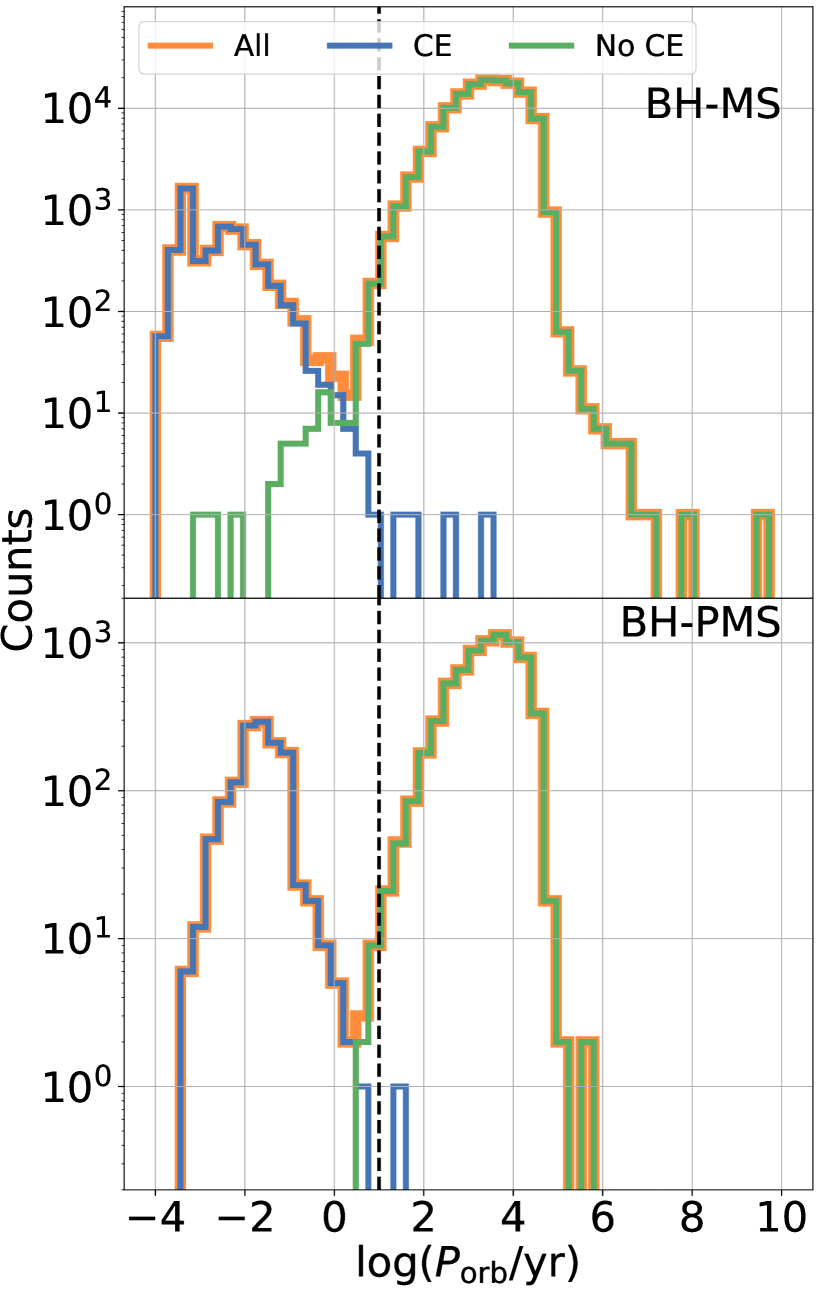
Figure 1: The distribution of orbital periods (${{P_{\rm{orb}}}}$) for all BH-LC binaries at present time in the Milky Way in our rapid model (section 2). The top and bottom panels show binaries with MS and PMS companions. Orange, blue, and green histograms denote distributions for all BH-LC binaries, those that went through at least one CE evolution, and those that never went through a CE evolution. The short-period peak is dominated by BH-LC systems created via at least one CE episode, whereas, the long-period peak is created primarily by BH-LC binaries that never went through a CE episode. In our analysis we consider BH-LC binaries with ${{P_{\rm{orb}}}}\leq 10\,{{\rm{yr}}}$ (the vertical black dashed line to guide the eye), such that a $10$-${{\rm{yr}}}$ Gaia mission can resolve the full orbit. Interestingly, $10$-${{\rm{yr}}}$ Gaia mission potentially can detect BH-LC binaries created via the CE channel as well as those that never went through a CE evolution. (The equivalent figure for our delayed model is presented in the Appendix.)

Figure 1 shows the overall distribution for the orbital periods (${{P_{\rm{orb}}}}$) of all BH-LC binaries in the Milky Way at present from the rapid model (section 2). The distribution of ${{P_{\rm{orb}}}}$ for BH-LC binaries in the delayed model is very similar (shown in the appendix). The ${{P_{\rm{orb}}}}$ distributions are clearly bimodal for both BH-MS and BH-PMS binaries for both of the adopted SN models. In both cases, the short-period peak is dominated by binaries created via at least one CE episode, whereas, the long-period peak is created primarily with BH-LC binaries that never undergo a CE. The location of the trough for all cases is between ${{P_{\rm{orb}}}}\sim 1$–$10\,{{\rm{yr}}}$. The majority ($\sim 96\%$) of BH-LC binaries with ${{P_{\rm{orb}}}}\leq 10\,{{\rm{yr}}}$ have gone through at least one CE evolution independent of the adopted SN mechanism. Interestingly, the extended $10\,{{\rm{yr}}}$ mission of Gaia allows sampling of the separation between the CE and non-CE peaks. While outside the scope of this work, future studies could investigate how the observed shape and width of the trough can constrain uncertain CE physics.

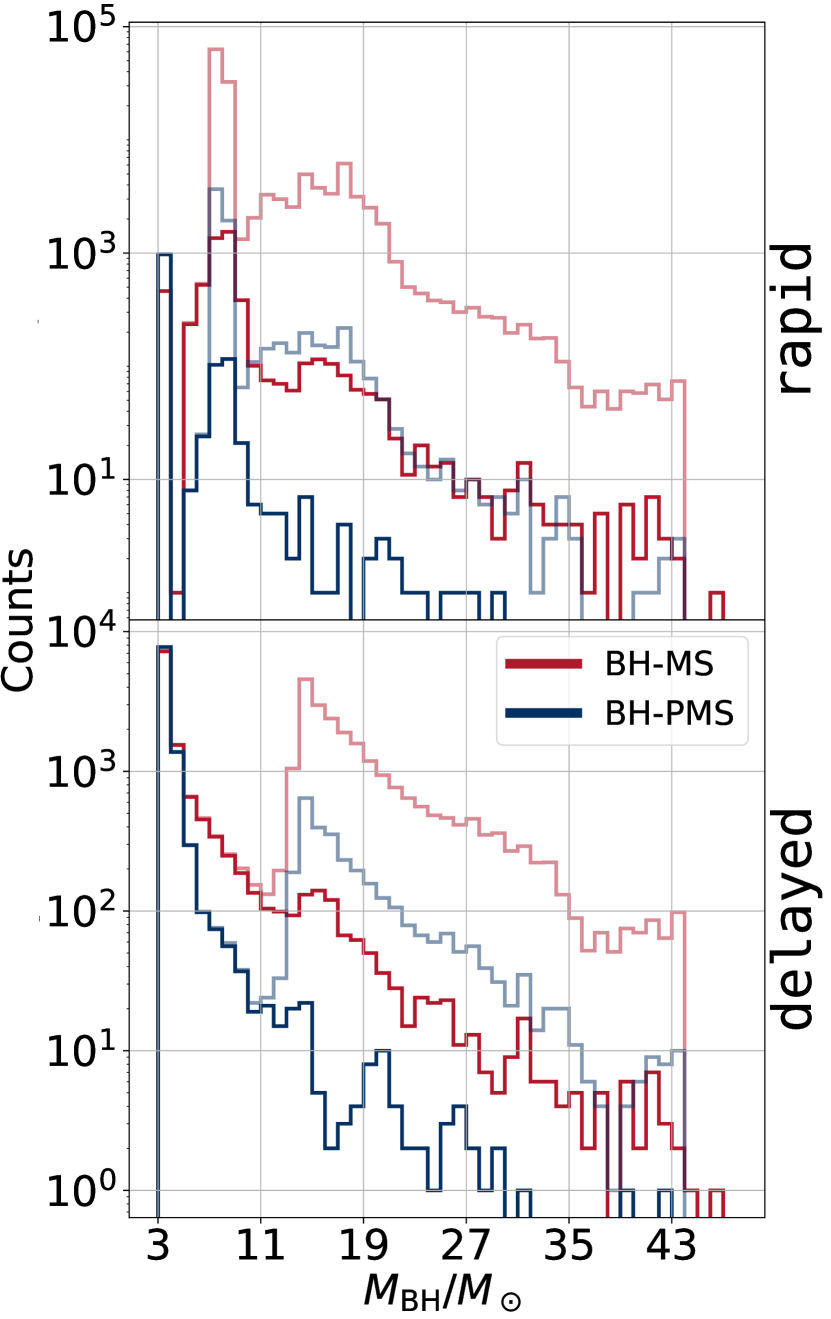
Figure 2: Distribution of BH mass for present-day populations from the rapid (top) and delayed (bottom) models. The blue and red curves represent MS and PMS companions, respectively. The faded and bright lines denote all BH-LC binaries without any constraints on ${{P_{\rm{orb}}}}$ and those satisfying ${{P_{\rm{orb}}}}\leq 10\,{{\rm{yr}}}$. The major difference between the two distributions come in the range ${{M_{\rm{BH}}}}/{M_{\odot}}=3$—$5$. In case of the rapid model, all BHs within ${{M_{\rm{BH}}}}/{M_{\odot}}=3$—$5$ come from AIC of NSs; we assume that the limiting mass for NSs is $3\,{M_{\odot}}$ (section 2). Whereas, for delayed, BHs formed via core-collapse SN can have masses down to $3\,{M_{\odot}}$. As a consequence, the delayed model consists of a relatively higher fraction [$25\ (71)\%$] of BHs in this mass range of compared to the rapid model [$0.3\ (12)\%$] with MS (PMS) companion. In both cases, ${{M_{\rm{BH}}}}$ is distributed in a wide range.

One of the most prominent differences between the two SN mechanisms manifests in the ${{M_{\rm{BH}}}}$ distribution; while the rapid prescription for core-collapse SN does not allow production of BHs in the mass range $3$ to $5\,{M_{\odot}}$, (often called the ‘mass-gap’ between neutron stars (NSs) and BHs), the delayed prescription predicts no mass gap. Figure 2 shows the ${{M_{\rm{BH}}}}$ distributions for BH-LC binaries at present day for the rapid and delayed models. The distributions are clearly different in the range between $3$ and $5\,{M_{\odot}}$, as expected. All BHs with ${{M_{\rm{BH}}}}$ between $3$ and $5\,{M_{\odot}}$ in the rapid model originate from accretion-induced collapse (AIC) of NSs. In contrast, in the delayed model, the AIC BHs contribute at $\sim 15\ (55)\%$ for BHs MS (PMS) companions and the rest come from core-collapse SN. The ${{M_{\rm{BH}}}}$ distribution continuous all the way down to ${{M_{\rm{BH}}}}/{M_{\odot}}=3$, our adopted mass that separates NSs from BHs in the delayed model, whereas, for the rapid model, there is a clear separation between the mass-gap BHs and the rest.

Interestingly, all BH-LC binaries with ${{M_{\rm{BH}}}}/{M_{\odot}}\lesssim 7$ ($10$) in the rapid (delayed) model have ${{P_{\rm{orb}}}}\leq 10\,{{\rm{yr}}}$ leading to identical populations for the BH-LC binaries with lower-mass BHs regardless of ${{P_{\rm{orb}}}}$ restrictions. This is because lower-mass BHs receive larger natal kicks in both SN prescriptions we have considered (Fryer et al., 2012) while for higher-mass BHs, natal kick magnitudes are reduced depending on the amount of mass that falls back onto the proto- compact object (e.g., Belczynski et al., 2008). The large natal kicks for low-mass BHs break their progenitor binaries with orbits ${{P_{\rm{orb}}}}/{{\rm{yr}}}\gtrsim 10$, while, the more massive counterparts in wide orbits can remain intact. If Gaia is able to characterize BHs in binaries with ${{M_{\rm{BH}}}}\sim 10\,{M_{\odot}}$ and ${{P_{\rm{orb}}}}\leq 10\,{{\rm{yr}}}$, strong constraints can be placed on the strength of natal kicks for these systems.

A few other features, originating from a combination of the adopted initial stellar mass function, metallicity and age distributions, and the complex binary star evolution of the initial population of binaries, are noticeable and different in the two models. For example, in the rapid model a peak in the range ${{M_{\rm{BH}}}}/{M_{\odot}}\approx 7$ to $9$ come from the evolution of metal-rich (${{\rm Z}}/{{\rm Z}}_{\odot}\geq 0.75$) systems. Another less prominent and broader peak between ${{M_{\rm{BH}}}}/{M_{\odot}}\approx 13$ and $19$ consists of systems that are relatively metal poor (${{\rm Z}}/{{\rm Z}}_{\odot}\leq 0.5$). In contrast, in the delayed model the distribution peaks near ${{M_{\rm{BH}}}}/{M_{\odot}}=3$ and again near ${{M_{\rm{BH}}}}/{M_{\odot}}\approx 15$.

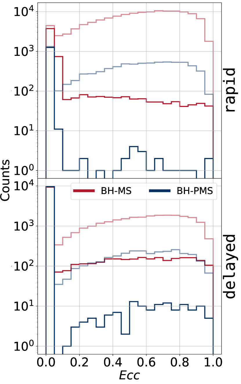
Figure 3: Same as Figure 2 but showing the distribution for the orbital eccentricities (${{Ecc}}$). In all cases there is a prominent peak for near-zero eccentricity, especially for BH-LC binaries with ${{P_{\rm{orb}}}}/{{\rm{yr}}}\leq 10$. This is because a large fraction of short-period BH-LC binaries go through CE evolution and are significantly affected by tides. The BH-MS (BH-PMS) binaries in the rapid and delayed models contain $0.8\%$ ($0.3\%$) and $7\%$ ($1\%$) ${{P_{\rm{orb}}}}/{{\rm{yr}}}\leq 10$ systems with $Ecc\geq 0.1$, respectively. The delayed model contains higher fraction of eccentric BH-LC binaries compared to the rapid model. This can be attributed to typically larger natal kicks in case of delayed. The fraction of near-circular orbits is less in case of BH-MS compared to BH-PMS in both models since tidal circularisation is more effective in BH-PMS binaries than in BH-MS binaries.

Figure 3 shows the distributions of BH-LC orbital eccentricities for the rapid and delayed models. We find that about $2\%$ ($15\%$) and $27\%$ ($76\%$) of BH-MS (BH-PMS) binaries with ${{P_{\rm{orb}}}}/{{\rm{yr}}}\leq 10$ have near-circular (${{Ecc}}\leq 10^{-2}$) orbits for the rapid and delayed models, respectively. The majority of the BH-LC systems with ${{P_{\rm{orb}}}}\leq 10\,{{\rm{yr}}}$ go through at least one CE evolution stage with the BH-progenitor’s envelope which circularizes the binary before BH formation (Figure 1). Moreover, even the small fraction of the short-period BH-LC binaries that never went through a CE phase can be significantly affected by tidal circularisation. In spite of this, the high fraction of eccentric BH-LC binaries primarily result from natal kicks during BH formation. The differences in the explosion mechanism between the rapid and delayed SN prescriptions lead to typically higher natal kicks in the delayed models. As a result, the fractions of short-period BH-MS (BH-PMS) binaries with significant ${{Ecc}}\geq 0.1$ are $0.8\%$ ($0.3\%$) and 7% (1%) in our rapid and delayed models, respectively. The connection between larger eccentricities and stronger natal kicks is a robust prediction that is independent of our chosen SN prescription. For both SN mechanisms, BH-PMS binaries usually have a smaller fraction of eccentric systems compared to BH-MS binaries, since the former have larger LC envelopes which are affected more strongly by tides after BH formation.

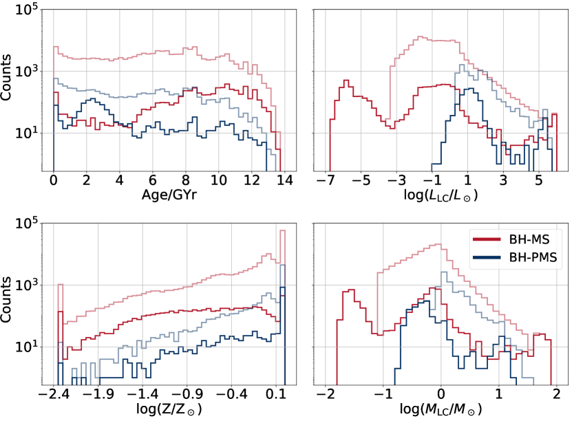
Figure 4: Distributions for present-day age (top-left), luminosity (top-right), metallicity (bottom-left), and mass (bottom-right) of the LC from our rapid model. Red and blue lines denote MS and PMS companions. The faded and bright lines denote all BH-LC binaries and those satisfying ${{P_{\rm{orb}}}}\leq 10\,{{\rm{yr}}}$, respectively. Simulated present-day BH-LC binaries in the Milky Way show large ranges in age, metallicity, ${{M_{\rm{LC}}}}$, and ${{L_{\rm{LC}}}}$. (The equivalent figure for our delayed model is presented in the Appendix.)

Figure 4 shows the distributions for age, metallicity, mass, and luminosity of the LCs for all BH-LC binaries and those satisfying ${{P_{\rm{orb}}}}\leq 10\,{{\rm{yr}}}$ for the rapid model. The corresponding figure for the delayed model is included in the Appendix. In contrast to the eccentricity and ${{M_{\rm{BH}}}}$ distributions, the LC properties primarily depend on the stellar IMF, binary stellar evolution physics, and the star formation and metallicity evolution in the Milky Way; they do not strongly depend on the details of the assumptions of core-collapse SN physics. As a result, the distributions of LC properties are very similar in the rapid and delayed models. We find that the ages of the BH-LC progenitors spans several Gyr covering the full range of the star particle ages in the galaxy model m12i. As a consequence, the BH-LC progenitors also have a wide range in metallicities. The pile up at the last metallicity bins near $\log({{\rm Z}}/{{\rm Z}}_{\odot})=-2.3$ and $0.2$ is simply because the star particles in the model galaxy m12i have a wider range in ${{\rm Z}}$ relative to the allowed ${{\rm Z}}$ range in COSMIC which is based on the single star fits of BSE (Hurley et al., 2000, see also the discussion in subsection 2.1). Nevertheless, the wide range in metallicities of our predicted present-day BH-LC binaries in the Milky Way indicates that if a sizeable population of BHs are detected, metallicity-dependent constraints on the properties of BHs may be obtained. Note that our earlier work made a simplifying assumption that used two fixed metallicity values corresponding to the thin and thick disks of the Milky Way (Breivik et al., 2017). Using more realistic metallicities that depend on the star-formation history in the Milky Way is one of the key improvements in the present study.

Almost all low-mass ($\lesssim 0.1\,{M_{\odot}}$) MS companions to the BH binaries show ${{P_{\rm{orb}}}}\leq 10\,{{\rm{yr}}}$. This is likely related to the CE evolution. Orbits with lower LC masses (on an average) contain a smaller reservoir of orbital energy to eject the envelope. As a result, BH’s with lower-mass LCs tend to have shorter post-CE orbits. Although, not as prominent, the same trend is observed for BH binaries with PMS companions; below ${{M_{\rm{LC}}}}\sim 1\,{M_{\odot}}$, all BH-PMS binaries have ${{P_{\rm{orb}}}}\leq 10\,{{\rm{yr}}}$.

A small ($\lesssim 0.1\%$) fraction of BH-MS binaries consist of MS stars in excess of $40\,{M_{\odot}}$. We find that in some cases, an initially high-mass ($M\geq 15\,{M_{\odot}}$) MS star accretes from the BH progenitor through stable mass transfer via RLOF and grow. These stars live longer than normal due to rejuvenation (e.g., Hurley et al., 2002). Most of these systems are also very young ($\lesssim 9\,{{\rm Myr}}$). As expected, the mass range for the PMS companions is narrower compared that for the MS companions because the PMS phase is a shorter-lived stage of evolution. In addition, lower-mass LCs must be sufficiently old to advance off the MS leading to a higher relative number of BH-MS binaries with ages larger than $6\,\rm{Gyr}$ relative to BH-PMS binaries.

We estimate that the Milky Way at present harbors $\sim 4\times 10^{5}$ ($\sim 8\times 10^{4}$) BH-LC binaries according to the rapid (delayed) model. Of these, $17,621^{+145}_{-144}$ ($29,616^{+181}_{-189}$) have ${{P_{\rm{orb}}}}/{{\rm{yr}}}\leq 10$. Of the BH-LC binaries with ${{P_{\rm{orb}}}}/{{\rm{yr}}}\leq 10$, $9,184^{+120}_{-133}$ ($7,091^{+113}_{-100}$) BH-LC binaries are in detached configurations in the rapid (delayed) model (Table 1). We focus on the detached BH-LC binaries with ${{P_{\rm{orb}}}}/{{\rm{yr}}}\leq 10$ in the Milky Way for Gaia’s ability to resolve the LC’s orbits throughout the rest of the paper.

4.2 BH-LC binaries in the Milky Way resolvable by Gaia

Table 1: BH-LC binaries in the Milky Way

Model	Type	Intrinsic			Resolvable
		All	${{P_{\rm{orb}}}}/{{\rm{yr}}}<10$		Optimistic			Pessimistic
			All	Detached	Resolved	$A_{v}$-corrected	BH candidate	Resolved	$A_{v}$-corrected	BH candidates
	MS	$369,199$	$14,679^{+142}_{-145}$	$8,658^{+113}_{-123}$	$383^{+33}_{-28}$	$255^{+19}_{-26}$	$76^{+9}_{-11}$	$191^{+20}_{-19}$	$139^{+12}_{-18}$	$35^{+8}_{-7}$
rapid	PMS	$18,990$	$2,947^{+52}_{-71}$	$529^{+26}_{-27}$	$88^{+11}_{-12}$	$36^{+9}_{-7}$	$31^{+8}_{-6}$	$47^{+9}_{-9}$	$14^{+5}_{-4}$	$12^{+4}_{-4}$
	total	$388,189$	$17,621^{+145}_{-144}$	$9,184^{+120}_{-133}$	$470^{+32}_{-30}$	$292^{+21}_{-26}$	$107^{+11}_{-12}$	$239^{+21}_{-20}$	$152^{+14}_{-17}$	$47^{+9}_{-8}$
	MS	$70,694$	$24,731^{+166}_{-175}$	$6,653^{+106}_{-104}$	$125^{+15}_{-12}$	$68^{+11}_{-9}$	$13^{+5}_{-4}$	$40^{+8}_{-8}$	$26^{+7}_{-6}$	$6^{+3}_{-3}$
delayed	PMS	$6,355$	$4,886^{+47}_{-48}$	$443^{+26}_{-28}$	$57^{+10}_{-8}$	$27^{+6}_{-7}$	$11^{+5}_{-3}$	$19^{+5}_{-5}$	$9^{+3}_{-4}$	$4^{+4}_{-2}$
	total	$77,049$	$29,616^{+181}_{-189}$	$7,091^{+113}_{-100}$	$184^{+15}_{-14}$	$95^{+12}_{-12}$	$24^{+7}_{-5}$	$60^{+8}_{-12}$	$36^{+7}_{-8}$	$10^{+4}_{-4}$

Note. — BH-LC numbers in the Milky Way predicted in our models. The numbers and errors denote the median and the spread between the $10$th and $90$th percentiles across the Milky-Way realisations. “Intrinsic” denotes the present-day population of BH-LC binaries in the Milky Way. “Resolvable” denotes the subset of BH-LC binaries resolvable by Gaia’s astrometry over a $10$ ${{\rm{yr}}}$ mission (subsection 3.2). Any detached BH-LC binary with ${{P_{\rm{orb}}}}/{{\rm{yr}}}\leq 10$ and resolved LC orbit is denoted as “Resolved.” “$A_{v}$-corrected” denotes the expected number of resolved BH-LC binaries after correcting for extinction and reddening from interstellar dust (subsection 3.1). A BH-LC is a “BH candidate” if Gaia’s astrometry can constrain the BH’s mass ${{M_{\rm{BH}}}}-\Delta{{M_{\rm{BH}}}}\geq 3\,{M_{\odot}}$ and ${{M_{\rm{BH}}}}\geq{{M_{\rm{LC}}}}$ within the $A_{v}$-corrected resolved population (subsection 3.3).

In this section we introduce the realistic Milky-Way populations each consistent with the complex and interdependent age-metallicity-Galactic position observed in the Galaxy (subsection 2.4). These realisations are different from each other in the random orientations, the distance, and the Galactic locations of the BH-LC binaries. As a result there are differences in the number of detections by Gaia in each realisation. These differences provide an estimate of the level of statistical fluctuations in the expected BH-LC numbers resolvable by Gaia.

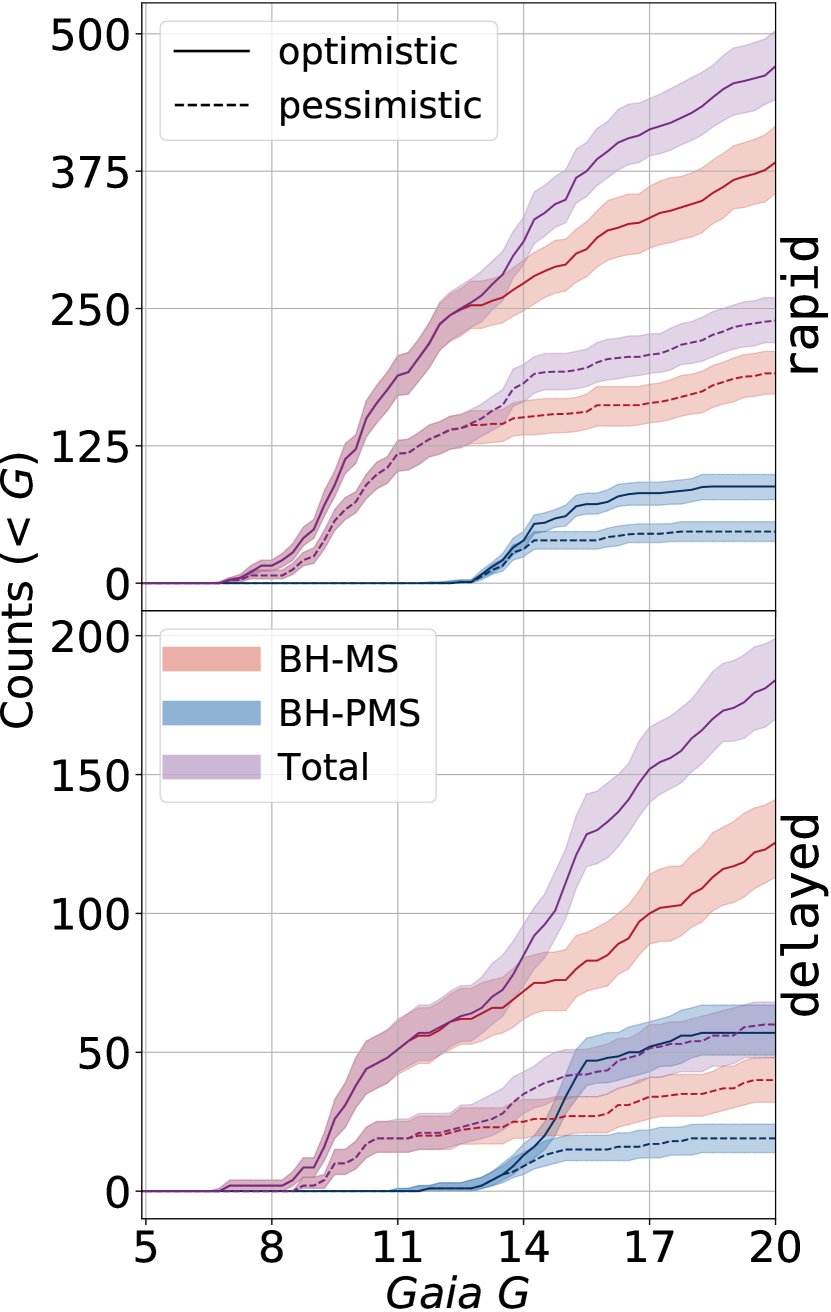
Figure 5: The cumulative number of expected detections of BH-LC binaries by Gaia as a function of Gaia’s $G$ magnitude for the rapid (top) and delayed models. Purple, blue, and red denote all BH-LC binaries, BHs with PMS, and MS companions, respectively. Lines and shaded regions around them represent the median and the range between the $10$th and $90$th percentiles. The statistical fluctuations come from the 200 realisations of the Milky Way we generate (subsection 2.4). Solid and dashed lines denote two different astrometric cuts, $\alpha>\sigma_{\xi}$ (optimistic) and $\alpha>3\sigma_{\xi}$ (pessimistic), respectively.

Figure 5 shows the cumulative number of BH-LC binaries for which Gaia can resolve the motion of the LC in orbit around the BH as a function of Gaia’s $G$ magnitude. The estimated total number of resolvable BH-LC binaries for the rapid model is between $\approx 240$ (pessimistic) and $470$ (optimistic). In case of the delayed model, the expected yield is lower, between about $60$ (pessimistic) and $185$ (optimistic) BH-LCs. The delayed SN prescription typically produces lower-mass BHs and higher natal kick magnitudes compared to the rapid SN prescription. As a result, a higher fraction of the progenitors of BH-LC binaries disrupt in our delayed model.

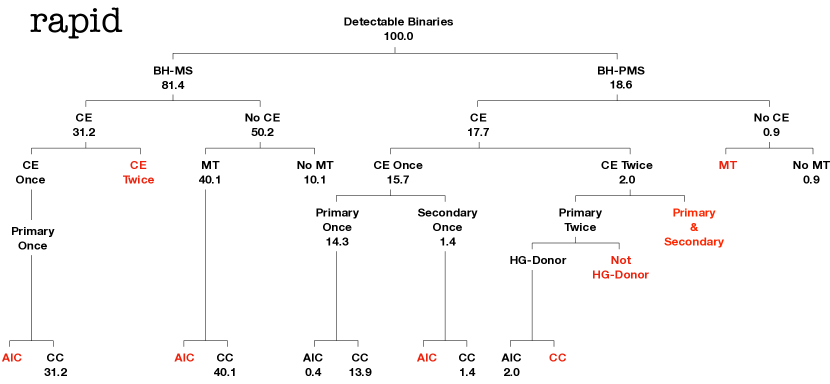
Figure 6: Branching ratios of the different formation channels for the resolvable BH-LC binaries in the rapid model. The branches in red denote no contribution from that channel. CE, MT, CC, and AIC denote common-envelope, stable mass transfer via RLOF, core-collapse SN, and accretion-induced collapse of a NS, respectively. We divide the CE channels based on the number of CE phases the binaries go through as well as the the binary component that initiates the CE. The fractional contribution from each channel is denoted by numbers in percent (rounded to one significant digit after the decimal). Most BH-LC binaries are BH-MS. We further highlight channels created via a HG donor, we allow such binaries to survive in our simulations. Note that BH-LC binaries that ever had a HG donor contribute towards BH-PMS at the level of about $2\%$.

We now embark on an investigation of the relative importance of various formation channels of the resolvable BH-LC binaries. Identification of the relative importance of different channels can inform which binary evolution physics of any particular channel matters most in estimating the model populations. In addition, different formation channels can create BH-LC binaries with significantly different properties including ${{P_{\rm{orb}}}}$ and ${{Ecc}}$ (Figure 1, 3). Moreover, future BH-LC detections from Gaia can inform the relative abundances of various types of BH-LC binaries and shed light on the uncertain aspects of binary stellar evolution including the CE, and BH formation physics.

Figure 6 and 7 show the detailed evolutionary pathways for the Gaia-resolvable BH-LC binaries and their relative importance. Below we mention the key findings. In case of the rapid model, above $80\%$ of resolvable BH-LC binaries are expected to contain a MS star as a companion. Overall, $\sim 50\%$ of all resolvable BH-LC systems come via CE evolution. Note that, the contribution from CE evolution in the intrinsic BH-LC population with ${{P_{\rm{orb}}}}/{{\rm{yr}}}\leq 10$ is much higher ($\sim 96\%$; subsection 4.1). However, Gaia’s astrometry can resolve the typically large orbits of the non-CE BH-LC binaries to larger distances. This selection bias increases the fraction of non-CE BH-LCs in the resolvable population. Looking at the resolvable BH-MS and BH-PMS populations separately, about $40\%$ ($95\%$) of the resolvable BH-MS (BH-PMS) binaries are expected to have undergone at least one CE phase.

Only about $2.4\%$ of the resolvable BH-LCs contain BHs formed via AIC and all of them have a PMS companion. This is significant in two ways. First, if the mass-gap is real, it will be easily discovered from the resolvable BH-LC population without any significant contamination from BHs created via AIC of NSs. Second, the resolvable BHs in the mass gap are expected to have PMS companions only.

We find that in about $2\%$ of the resolvable BH-LCs the BH progenitor is the donor while crossing the Hertzsprung Gap (HG) during one of the CE episodes. Whether a binary can survive a phase of CE evolution with a HG donor is uncertain(e.g., Ivanova & Taam, 2004; Belczynski et al., 2008). In spite of the uncertainty of this channel, we do not exclude these systems from our analysis for the sake of completeness. Interestingly, if we do exclude systems that underwent a CE initiated by a HG donor, then the fraction of resolvable BH-LCs containing mass-gap BHs reduces to only $0.4\%$.

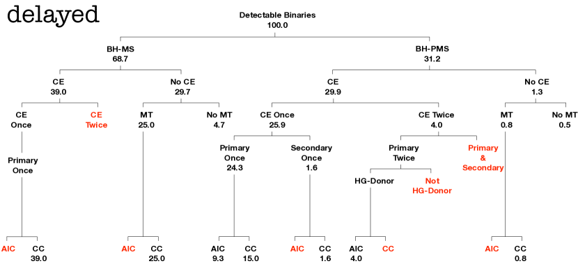
Figure 7: Same as Figure 6, but for the delayed model. BH-MS and BH-PMS created via CE evolution have similar contributions. BH-LCs that at some point had a HG donor contributes at the level of about $4\%$.

In the delayed model, the relative importance of the formation channels are somewhat different. MS companions still dominate ($69\%$) the population of resolvable BH-LCs. About $70\%$ of the resolvable BH-LCs form via at least one CE episode and about $13\%$ of the BH-LCs contain BHs created via AIC.

The extension of Gaia’s mission from $5$ to $10$ years allows Gaia to target BH-LCs up to ${{P_{\rm{orb}}}}=10\,{{\rm{yr}}}$ and still resolve the full orbit. According to our rapid (delayed) model, the total expected yield of resolved BH-LC binaries increases by $34\%$ ($16\%$) simply because of the mission extension and this increase in overall yield almost entirely comes from the increase in detectability of longer-period BH-LC binaries that do not go through CE evolution. We find that Gaia’s $10\,{{\rm{yr}}}$ mission would identify significant fractions ($50\%$ and $30\%$ for rapid and delayed models) of resolvable BH-LC binaries that do not come from the CE evolution channel. If such yields are realised, it may be possible to distinguish resolved BH-LC systems that form via CE evolution from those that do not simply using the ${{P_{\rm{orb}}}}$ distribution.

4.3 Key Properties of resolvable BH-LC binaries

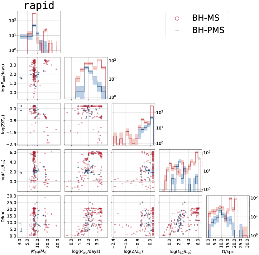
Figure 8: Corner plot showing the observable properties- ${{L_{\rm{LC}}}}$, $D$, ${{\rm Z}}$, ${{P_{\rm{orb}}}}$, and ${{M_{\rm{BH}}}}$- of BH-MS (red) and BH-PMS (blue) binaries resolvable by Gaia in our rapid model. The scatter plots show each unique resolvable binary across all of our Milky Way realisations. Histograms denote the PDF for each property. The shaded regions in the histograms have the same meaning as in Figure 5.

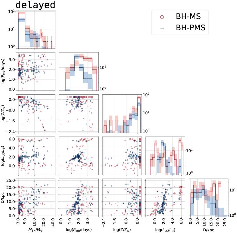
Figure 9: Same as Figure 8 but for the delayed model.

In this section we highlight some key properties of the resolvable BH-LC binaries. Comparisons between the distribution of properties presented here with those presented in subsection 4.1 sheds light on the selection biases of Gaia. Figure 8 and 9 show the corner plots for all resolvable binaries across all Milky Way realisations from our rapid and delayed models. Note that different Milky Way realisations can sample the same binaries multiple times (subsection 2.4). To avoid clutter, we plot resolvable binaries in the scatter plots only once and ignore the repeated draws. However, we create the histograms taking into account the repeated draws.

The difference between the rapid and delayed models manifests most prominently for BHs with $3\leq{{M_{\rm{BH}}}}/{M_{\odot}}\leq 5$. In the rapid (delayed) model, about $2.4\%$ ($65\%$) of the resolvable BH-LCs contain BHs in this mass range. If we discard the systems that have undergone CE involving a HG donor, the contrast is even starker. For resolved BH-LCs with BHs in this mass range, while in the rapid model we do not find any BH-MS binaries, in the delayed model BH-MS and BH-PMS contribute almost equally. Note that, even in the delayed model AIC BHs contribute only at about $13\%$ within this ${{M_{\rm{BH}}}}$ range and the rest come from core-collapse SN. We already highlighted similar trends in Figure 2 in the context of the intrinsic population of BH-LCs, however, it is interesting that this difference is prominent in the resolvable population as well. Detection of BHs with $3\leq{{M_{\rm{BH}}}}/{M_{\odot}}\leq 5$ with both MS and PMS companions in detached configuration would clearly indicate that the so-called mass-gap from core-collapse SN may not be real. Indeed, the recent discovery of BH-LC candidates with BH masses in this range (Thompson et al., 2019; Jayasinghe et al., 2021) and microlensing analyses (Wyrzykowski & Mandel, 2020) provide observational evidence against the existence of a mass gap.

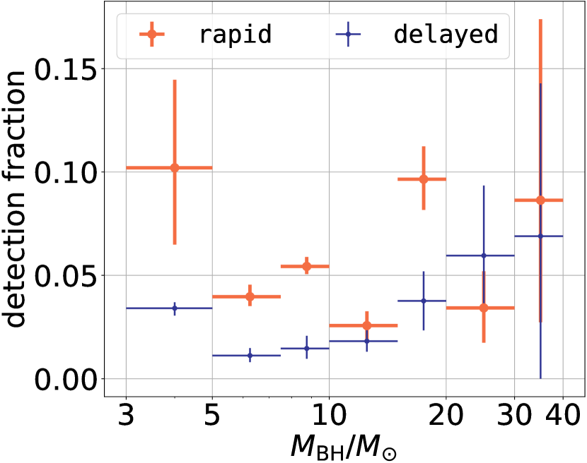
Figure 10: The ratio between the Gaia-resolvable and the intrinsic numbers of detached BH-LC binaries with ${{P_{\rm{orb}}}}/{{\rm{yr}}}\leq 10$ in the Milky Way as a function of ${{M_{\rm{BH}}}}$. Orange and blue denote rapid and delayed models. The horizontal and vertical errorbars denote the ${{M_{\rm{BH}}}}$ bin span for the calculation and range between the 10th and 90th percentiles, respectively. We do not find a strong correlation between Gaia’s ability to resolve a BH-LC binary and ${{M_{\rm{BH}}}}$.

It is interesting that the shapes of the ${{M_{\rm{BH}}}}$ distributions in our models do not change significantly between the intrinsic and resolvable populations of BH-LC binaries in the Milky Way independent of the adopted SN prescription. This indicates that the ability for Gaia to resolve a BH-LC binary do not strongly depend on ${{M_{\rm{BH}}}}$. Indeed, we find that the ratio between the total numbers of BH-LC binaries in the Milky Way and those that are resolvable by Gaia, do not strongly correlate with ${{M_{\rm{BH}}}}$ (Figure 10). This is because Gaia’s astrometric selection biases do not depend directly on the BH, rather they depend on the LC and orbital properties, such as $G$ and ${{P_{\rm{orb}}}}$. As a result, the population of BHs resolvable by Gaia is expected to exhibit ${{M_{\rm{BH}}}}$-distribution that is very close to the intrinsic one in the Milky Way.

The other potentially observable difference between the BH-LCs in the rapid and delayed models stems from the differences in the fallback-dependent natal kicks in the two respective SN mechanisms. The majority of the resolvable systems- about $90\%$ ($95\%$) in the rapid (delayed) model- go through dissipative binary evolution phases such as CE evolution and RLOF. The final eccentricities are almost entirely dependent on the natal kicks the BHs receive modulated later by tidal cirularisation or RLOF. Because of this, in both the rapid and delayed models, there are prominent peaks near circular orbits. We find that about $87\%$ ($33\%$) of the resolvable BH-LC binaries have ${{Ecc}}\leq 0.1$ in the rapid (delayed) model. Similar to the intrinsic population, the resolvable BH-MS binaries in the delayed model show a higher fraction of eccentric systems compared to those in the rapid model. We find that the resolvable systems with ${{Ecc}}\geq 0.5$ in both rapid and delayed models form predominantly from progenitor binaries that never underwent a CE evolution. Since, this group also consists of relatively wider orbits, they are also less affected by tides after BH formation. In both models, the fraction of eccentric BH-MS binaries is higher than that of eccentric BH-PMS binaries in the resolvable population since the BH-PMS binaries are more strongly affected by tides. Thus future observations of the eccentricity distribution of BH-LC binaries can put constraints on the natal kick strengths for stellar-mass BHs. Such constraints would be complimentary to those based on the locations of BH XRBs away from the Galactic plane (e.g., Repetto et al., 2012; Repetto & Nelemans, 2015) or those coming from detailed modeling of individual observed BH XRBs (e.g., Brandt et al., 1995; Gualandris et al., 2005; Fragos et al., 2009; Wong et al., 2014).

Similar to the intrinsic population in the Milky Way, the resolvable population also shows a wide range in metallicities. We also find an expected anti-correlation between metallicity and ${{M_{\rm{BH}}}}$ since metallicity-dependent stellar winds strongly reduce the maximum BH mass for near solar metallicities (e.g., Belczynski et al., 2010). Several other expected correlations are apprent in Figure 8 and 9. For example, longer-period binaries are detected at further distances; all resolvable detached BH-LC binaries reside right of a line representing the limiting angular size of the orbit. Similarly, brighter systems are detected at higher distances. In contrast, no clear correlation is found between ${{M_{\rm{BH}}}}$ and the distance to the resolvable binary. Some other relations, for example between distance and metallicity, simply come from the fact that we have used initial conditions such that the complex dependence between age-metallicity-distance in the Milky Way is preserved (subsection 2.1).

4.4 Effects of Reddening

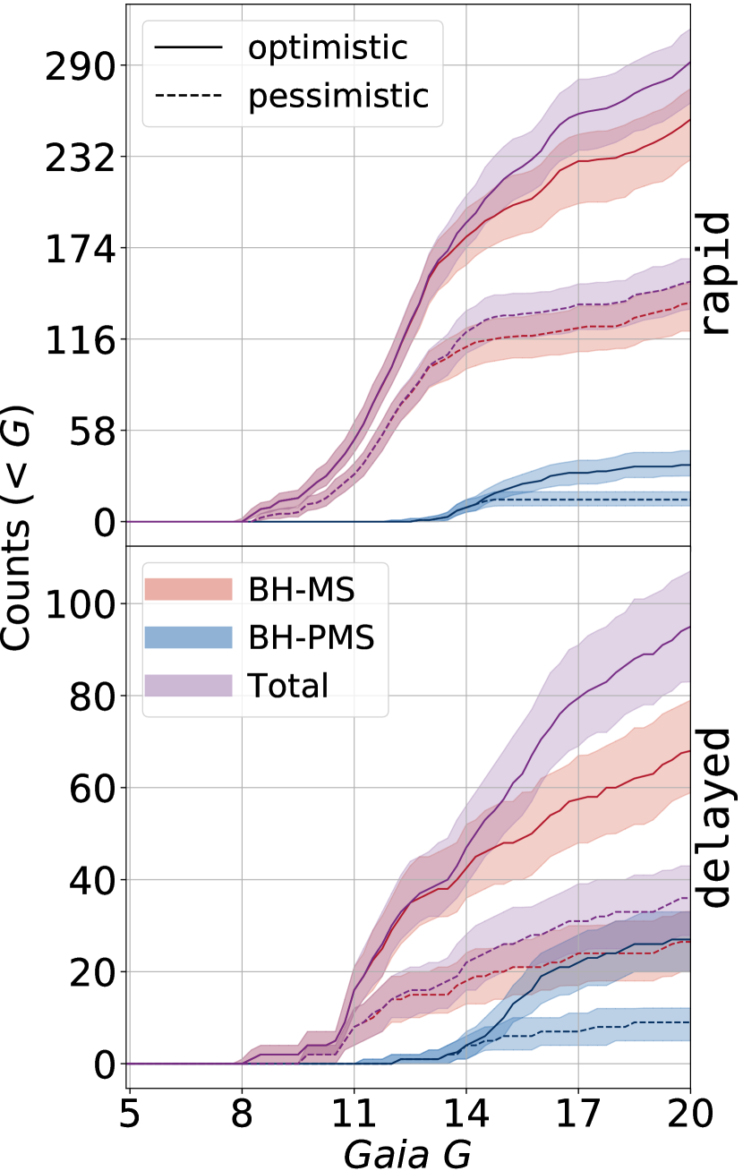
Figure 11: Cumulative number of Gaia-resolvable BH-LC binaries after incorporating the effects of extinction and reddening. The line-styles, colors, and the shades have the same meaning as in Figure 5. After correcting for extinction and reddening, the expected number of detections is between $\approx 36$ (delayed model with pessimistic cut) $292$ (rapid model with optimistic cut). We find a higher expected yield for the rapid model compared to the delayed model by a factor of about $3.0$ ($4.2$) using the optimistic (pessimistic) cut. This difference can be attributed to typically lower-mass BHs and larger kicks in case of delayed.

In this section we evaluate the effects of reddening on our estimated yield of detached BH-LC binaries by Gaia. The details of our method to determine extinction and reddening ar described in subsection 3.1. Figure 11 shows the expected number of detections as a function of Gaia’s $G$ magnitude after taking into account the effects of extinction and reddening. We find that reddening and extinction significantly decreases the expected number of detections (Table 1). After correcting for reddening and extinction we estimate that Gaia would resolve between $292^{+21}_{-26}$ (optimistic) and $152^{+14}_{-17}$ (pessimistic) BH-LCs in the rapid model. Whereas, the corresponding numbers for the delayed model are $95^{+12}_{-12}$ (optimistic) and $36^{+7}_{-8}$ (pessimistic). Our extinction- and reddening-corrected estimate for the BH-LC binaries resolvable by Gaia provide the most realistic estimates for detection yields. Thus, in the following sections we proceed with the extinction- and reddening-modulated resolvable systems.

4.5 Possible astrometric constraints on ${{M_{\rm{BH}}}}$

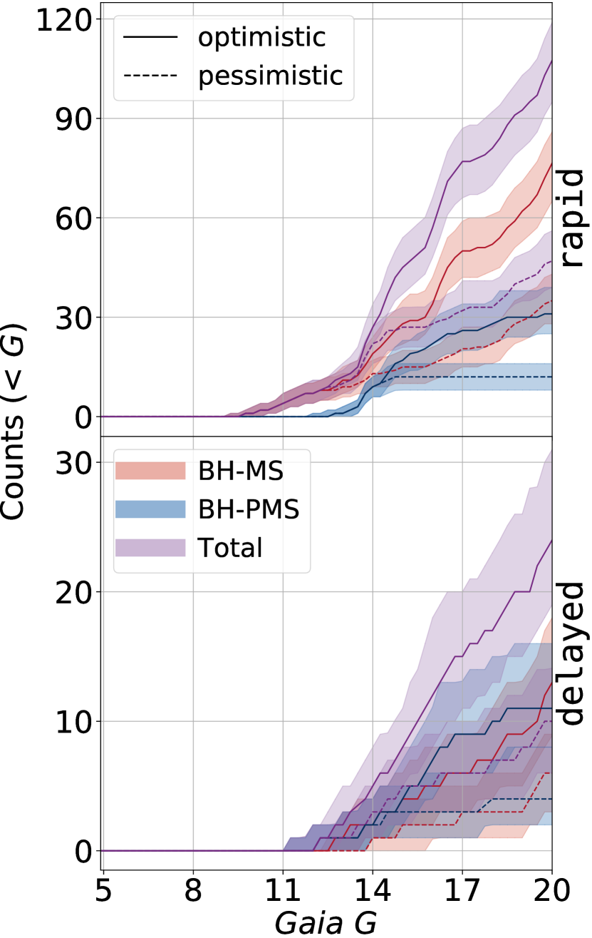
Figure 12: Same as Figure 11, but after imposing the additional constraints, ${{M_{\rm{BH}}}}-\Delta{{M_{\rm{BH}}}}\geq 3\,{M_{\odot}}$ and ${{M_{\rm{BH}}}}\geq{{M_{\rm{LC}}}}$ on the extinction- and reddening-corrected detection numbers. We call this subset BH candidates. We estimate $\Delta{{M_{\rm{BH}}}}$ from subsection 3.3. We assume, on an average, $10\%$ error in estimating ${{M_{\rm{LC}}}}$. These numbers indicate the number of cases where Gaia’s astrometry of the LC alone can identify that the dark companion must be a BH.

In this section we investigate whether Gaia’s astrometry alone can clearly identify the nature of an unseen dark companion to an observed LC as a BH via mass constraints with sufficient accuracy. Note that, in our analysis, the LC exclusively dominates the emission observed by Gaia. Hence, a higher-mass unseen object is most likely to be a dark remnant. This essentially means that if Gaia’s astrometry can provide mass constraints that clearly indicate that an unseen companion is more massive than any NSs or the LC mass, it must be a BH candidate.

By Gaia’s final data release, the parallax to identified binaries will be supplied. As a result, the absolute luminosity and hence the mass of the LC can be constrained from the Gaia magnitudes using standard stellar evolution models (e.g., Anders et al., 2019; Howes et al., 2019). The constrained mass of the LC and the determined ${{P_{\rm{orb}}}}$ from Gaia astrometry can then provide constraints for the unseen dark remnant in the binary. In Andrews et al. (2019) we showed that this is possible and the accuracy in the mass measurement for the dark component depends on the accuracy in the mass measurement of the LC and the accuracy of the along and across scans for the source. The analytic expression and the details of the calculation for mass errors of the BHs are given in subsection 3.3.

In order to find the subset of BH-LC binaries where Gaia’s astrometry alone can reveal that the dark remnant is a BH, in addition to all of Gaia’s detectability considerations (subsection 3.2) and effects of extinction and reddening (subsection 3.1), we employ two additional filters, (i) ${{M_{\rm{BH}}}}>{{M_{\rm{LC}}}}$ and (ii) ${{M_{\rm{BH}}}}-\Delta{{M_{\rm{BH}}}}\geq 3\,{M_{\odot}}$. The former condition is to rule out confusion potentially created by very high-mass bright primary in orbit with another less bright secondary of mass above $3\,{M_{\odot}}$ in observed systems. We denote this subset as BH candidates. Note that our constraint of ${{M_{\rm{BH}}}}-\Delta{{M_{\rm{BH}}}}\geq 3\,{M_{\odot}}$ is conservative and consistent with the assumed boundary between NSs and BHs in our simulations. We do not suggest that NSs can be as massive. The estimated masses of the heavy NSs to date are lower than $3\,{M_{\odot}}$ (e.g., Cromartie et al., 2020; Biswas et al., 2021).

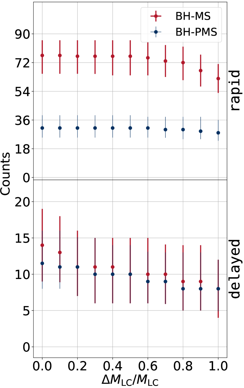
Figure 13: Number of BH candidates as a function of the adopted value of $\Delta{{M_{\rm{LC}}}}/{{M_{\rm{LC}}}}$. Red (blue) dots and errorbars denote the median, and the range between the 10th and 90th percentiles for BH-MS (BH-PMS) binaries. The number of BH candidates remains within the levels of statistical fluctuations throughout the full range in $\Delta{{M_{\rm{LC}}}}/{{M_{\rm{LC}}}}$.

Figure 12 shows the expected number of BH-LC binaries as a function of Gaia’s $G$ magnitude, where astrometry alone can determine that the mass of the unseen primary to a secondary LC is $\geq 3\,{M_{\odot}}$. We find that all of the above stringent criteria are satisfied for $\approx 37\%$ ($25\%$) of reddening-corrected resolvable systems in the rapid (delayed) model. According to our optimistic threshold for Gaia’s astrometric precision, the total numbers of resolvable BH-LC binaries with astrometric mass measurements strongly indicating a BH as the dark object, is $107^{+11}_{-12}$ ($24^{+7}_{-5}$) for the rapid (delayed) model. Based on the pessimistic threshold, the corresponding number is $47^{+9}_{-8}$ ($10^{+4}_{-4}$) (Table 1).

While the results shown in Figure 12 uses the fiducial value $\Delta{{M_{\rm{LC}}}}/{{M_{\rm{LC}}}}=0.1$, we note that the precision in mass estimates of isolated single or binary stars can vary widely depending on the system, data quality, as well as the measurement technique (e.g., Torres & Ribas, 2002; Gallenne et al., 2016; Pavlovski et al., 2018; Brogaard et al., 2018; Rendle et al., 2019). Our subsection 3.3 provides a straightforward way to use any desired value of $\Delta{{M_{\rm{LC}}}}/{{M_{\rm{LC}}}}$ to ultimately update the estimated $\Delta{{M_{\rm{BH}}}}/{{M_{\rm{BH}}}}$ through Gaia’s astrometry. Nevertheless, by varying $\Delta{{M_{\rm{LC}}}}/{{M_{\rm{LC}}}}$ between the full range of zero and one, we find that the estimated number of BH candidates do not depend strongly on the chosen value of $\Delta{{M_{\rm{LC}}}}/{{M_{\rm{LC}}}}$ (Figure 13). In fact, throughout the full range, the estimated numbers stay within the range due to statistical fluctuations for any one of the chosen values of $\Delta{{M_{\rm{LC}}}}/{{M_{\rm{LC}}}}$ including our fiducial value of 0.1. The lack of sensitivity towards the adopted value of $\Delta{{M_{\rm{LC}}}}/{{M_{\rm{LC}}}}$ can be easily understood from subsection 3.3. To identify BH candidates, we impose the condition ${{M_{\rm{BH}}}}\geq{{M_{\rm{LC}}}}$. This makes the term involving $\Delta{{M_{\rm{BH}}}}/{{M_{\rm{BH}}}}$ less significant compared to the other term involving astrometric precision.

5 Promise from followup measurements beyond astrometry

While our primary focus of this work is on the ability of Gaia to detect and characterise detached BH-LC binaries using astrometry alone, of course, once identified by Gaia’s astrometry, followup observations of these binaries can significantly improve the characterisation of the binary properties. In this section we highlight a couple of these promising avenues.

5.1 Radial velocities using Gaia’s spectroscopy

The most readily available avenue to improve characterisation of astrometrically identified candidates of interest is RV measurements by Gaia itself. Gaia contains a RV spectrometer which provides spectral resolution $R\sim 5000$ (low) and $R\sim 11500$ (high) for stars with $G\leq 17$ and $G\leq 11$, respectively. We find that Gaia’s high-$R$ spectra may not be very useful in characterising BH-LC binaries. While the high-$R$ allows measurement of lower RV semiamplitudes ($K$), the stronger constraint on $G$ prohibitively limits the number of available BH-LC binaries in the Milky Way.

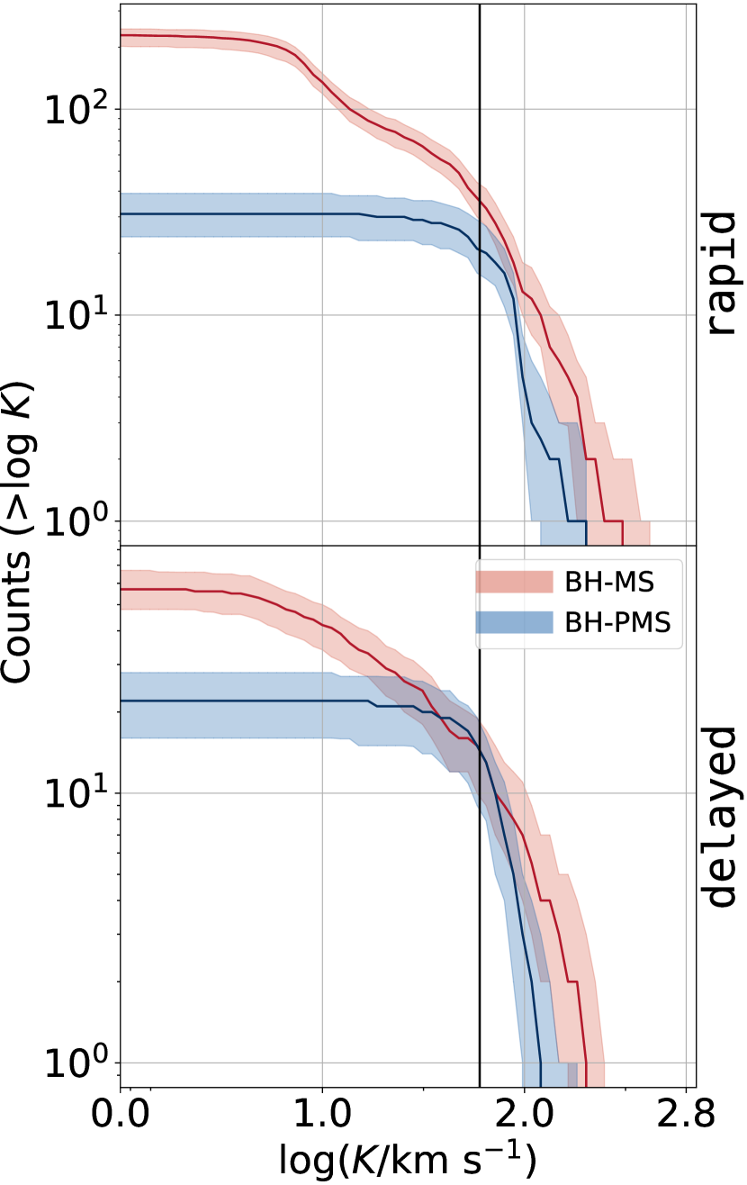
Figure 14: Reverse cumulative distribution of the RV semi-amplitude ($K$) for detached BH-LC binaries resolvable by Gaia (using the optimistic threshold for astrometric resolution) with $G<17$ after correcting for extinction and reddening. The vertical line denotes the level of $K$ resolved by Gaia’s low spectral resolution ($R$) data. Red and blue denote BH binaries with MS and PMS companions. Lines and shaded regions around the lines denote the median and the spread between the 10th and 90th percentiles.

Figure 14 shows the distribution RV semiamplitude ($K$) for the reddening- and extinction-corrected, resolvable BH-LC binaries with $G<17$. We find that in the rapid model $\sim 35$ BH-MS and $21$ BH-PMS binaries could have high enough $K$ to be resolved by Gaia’s low-$R$ spectroscopy (Figure 14). In comparison, in the delayed model $\sim 14$ BH-MS and $\sim 15$ BH-PMS binaries are expected to have high enough $K$ to be resolved by Gaia’s low-$R$ spectra. Using Gaia’s high-$R$ spectra, these numbers are at most a few in both rapid and delayed models. As can be seen in Figure 14, $K$ for Gaia-resolvable BH-LC binaries is rather large. Hence, a compromise in the spectral resolution matters less than the loss of available systems in the Milky Way from a stronger constraint in $G$.

Overall, we find that a little over $35\%$ of the detached Gaia-resolvable (reddening-corrected) BH-LC binaries will have some constraints on ${{M_{\rm{BH}}}}$ either through astrometry (as described in subsection 4.5) or through RV measurements using Gaia’s low-$R$ spectra. Although, we limit our discussion to RV measurements using Gaia’s spectrometer, of course, once the BH binary candidates are identified, a higher fraction of systems may be constrained via RV followup using other higher-$R$ telescopes that can probe fainter stars. We also caution the readers that in our quick analysis we did not consider the details that affect the feasibility of RV measurements of a particular LC which include availability of lines to observe within the band of the spectrometer, Galactic position, and stellar activity.

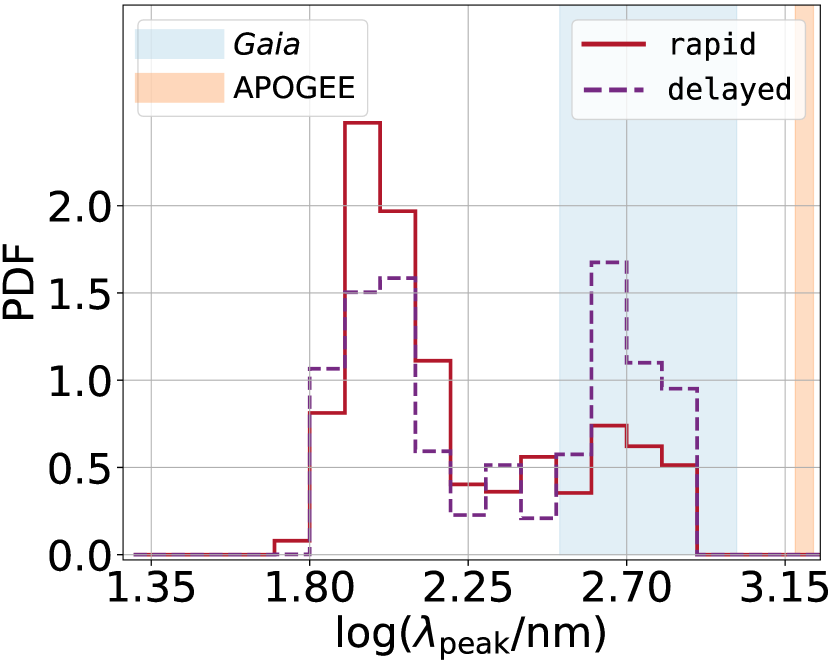
Figure 15: Distribution of the wavelengths ($\lambda_{\rm{peak}}$) corresponding to the peak in the blackbody spectral-energy distribution for the resolvable rapid (red) and delayed (purple) binaries. Blue and orange vertical bands show the ranges of bandpass filters for Gaia ($330$–$1050\,\rm{nm}$) and APOGEE ($1.51$–$1.70\,\micron$). The wavelength band for Gaia is more favorable for the majority of the BH-LC binaries compared to that of APOGEE.

Till date the discovered detached BH-LC binaries have used data from multi-epoch spectroscopic surveys by the MUSE (e.g., Giesers et al., 2018, 2019) and APOGEE collaborations (e.g., Thompson et al., 2019; Jayasinghe et al., 2021). MUSE specifically focuses in crowded fields such as globular clusters, whereas, primary APOGEE targets are in the field. Hence, it is interesting to compare Gaia’s capabilities with that of APOGEE in the context of detecting BH-LC binaries using RV measurements. In order to find the number of Gaia-resolvable BH-LC binaries APOGEE may also detect, we take the subset of reddening-corrected Gaia-resolvable BH-LC binaries in our models and apply two additional filters relevant for APOGEE. In particular, we use $J-K_{s}\leq 0.5$ and $12.2\leq H\leq 14$ (Zasowski et al., 2013; Price-Whelan et al., 2020). We find that APOGEE cannot detect any BH-MS binaries in our Gaia-resolvable populations and may detect $\sim 1$ ($\sim 3$) BH-PMS binaries in the rapid (delayed) model. Note that, both APOGEE detections of BH candidates so far contain PMS companions (e.g., Thompson et al., 2019; Jayasinghe et al., 2021). The reason why Gaia is expected to be more prolific in discovering BH-LC candidates, especially, BH-MS binaries, can be understood by comparing the filters of Gaia and APOGEE (Figure 15). APOGEE is sensitive to much cooler stars compared to Gaia. Most of the detached BH-LC binaries that Gaia can resolve are too faint in APOGEE.

5.2 X-ray counterparts

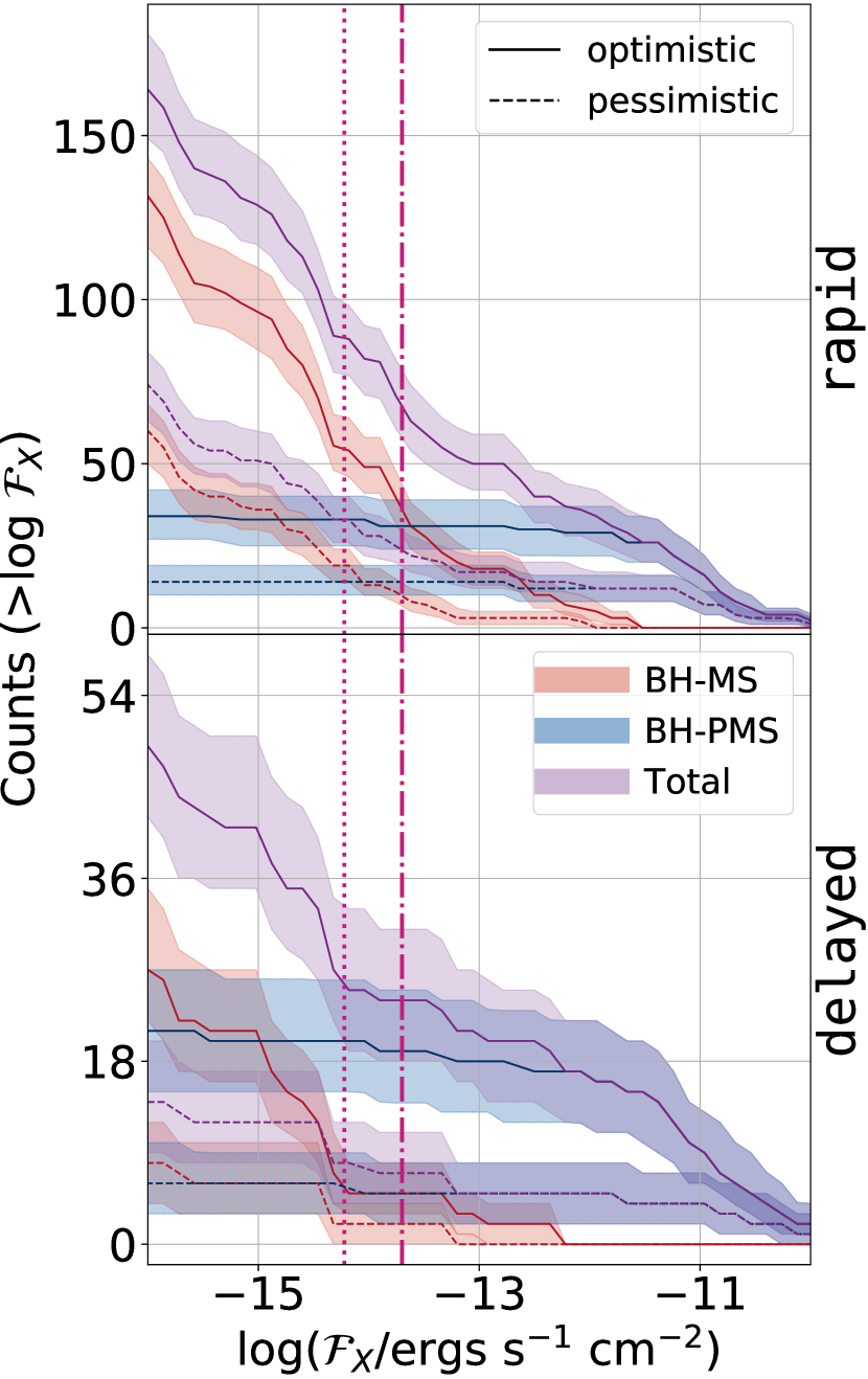
Figure 16: Reverse cumulative distributions of reddening-corrected, resolvable, detached BH-LC binaries as a function of the extinction and reddening corrected X-ray flux $\mathcal{F}_{\rm{x}}$ in the band $0.1-10{\rm{keV}}$. All systems shown here are wind-fed systems. The vertical pink lines denote $\mathcal{F}_{X}=6\times 10^{-15}\,{{\rm{ergs\ s^{-1}}}}\ {\rm{cm^{-2}}}$ (dotted) and $\mathcal{F}_{X}=2\times 10^{-14}\,{{\rm{ergs\ s^{-1}}}}\ {\rm{cm^{-2}}}$ (dash-dot), our adopted lower limits for detectability by Chandra and eROSITA, respectively. Red, blue, and purple denote BH-MS, BH-PMS, and all BH-LC binaries. Top and bottom panels are for the rapid and delayed models.

A fraction of the reddening-corrected, resolvable, detached BH-LC binaries may have X-ray counterparts if the stellar wind from the LC is accreted by the BH at a sufficiently high rate. We can estimate the bolometric X-ray luminosity for these wind-fed systems as-

$$L_{X}=\varepsilon\frac{G{{M_{\rm{BH}}}}\dot{M}_{\rm{acc}}}{R_{\rm{acc}}},$$ (13)

where $\dot{M}_{\rm{acc}}$ is the accretion rate of the BH, ${R_{\rm{acc}}}$ is the accretion radius, and $\varepsilon$ is an efficiency parameter for the conversion of gravitational binding energy to radiation. For our calculations we assume, ${R_{\rm{acc}}}\approx 3\times R_{\rm{sc}}$ ($R_{\rm{sc}}$ is the Schwarzschild radius) and $\dot{M}_{\rm{acc}}\sim 10^{-12}$ – $10^{-8}\,{M_{\odot}}\ {{\rm{yr}}}^{-1}$. Since $\dot{M}_{\rm{acc}}$ for the resolvable binaries is expected to be low, $\leq 10\%$ of the Eddington rate, we adopt that the accretion process is in the regime of the advection dominated accretion flow (ADAF). We adopt the prescription given in Xie & Yuan (2012, their equation 11) to calculate the efficiency parameter. In particular, assuming the viscosity parameter $\alpha=0.1$, viscous heating parameter $\delta=0.5$, we find $\varepsilon$ ranges from $10^{-5}-0.082$ based on the ratio of $\dot{M}_{\rm{acc}}$ to the Eddington mass accretion rate.

We assume that the bolometric X-ray luminosity calculated using Equation 13 includes X-rays in the energy range $0.1-500{\rm{keV}}$. Since X-ray observatories like Chandra and eRosita are sensitive in the energy band $0.1-10{\rm{keV}}$, we evaluate the incident flux $\mathcal{F}_{\rm{X}}$ in the energy band $0.1-10{\rm{keV}}$ assuming a power law spectrum for X-rays,

$$N(E)\propto E^{-\Gamma},$$ (14)

with photon index $\Gamma=2$ (Yang et al., 2015). Furthermore, we correct $\mathcal{F}_{\rm{X}}$ for interstellar extinction and reddening using

$$\mathcal{F}_{\rm{X}}=\int_{0.1}^{10}e^{\sigma_{\rm{ISM}}(E)N_{H}}EN(E)\,dE$$ (15)

where $\sigma_{\rm{ISM}}(E)$ is the total photoionization cross section of ISM taken from Wilms et al. (2000), and $N_{\rm{H}}$ is the hydrogen column density between the source and the observer. We estimate $N_{\rm{H}}$ simply from the position-dependent $A_{v}$ obtained using mwdust:

$$\frac{N_{H}}{A_{v}}=2.2\times 10^{21}{\rm{cm}}^{-2}$$ (16)

(Güver & Özel, 2009).

We show the reverse cumulative numbers of reddening-corrected Gaia-resolvable detached BH-LC binaries as a function of $\mathcal{F}_{X}$ in Figure 16. We adopt, the detection limits of Chandra and eROSITA as $\mathcal{F}_{X}\geq 6\times 10^{-15}\,{{\rm{ergs\ s^{-1}}}}\ {\rm{cm^{-2}}}$ (based on CSC2.0 catalog Weisskopf et al., 2000) and $\mathcal{F}_{X}\geq 2\times 10^{-14}\,{{\rm{ergs\ s^{-1}}}}\ {\rm{cm^{-2}}}$ (Merloni et al., 2012), respectively. We find that the number of reddening-corrected, Gaia-resolvable, detached BH-LC binaries expected to have X-ray counterparts in eROSITA are $68^{+9}_{-10}$ ($24^{+6}_{-5}$) and $24^{+7}_{-6}$ ($7^{+4}_{-3}$) for the rapid and delayed models adopting the optimistic (pessimistic) astrometric threshold. The corresponding numbers for Chandra are $88^{+11}_{-11}$ ($33^{+7}_{-7}$) and $25^{+8}_{-6}$ ($8^{+4}_{-4}$), respectively. Interestingly, although further characterisation is needed to ascertain the nature of these sources several studies have reported possible BH-LC candidates by cross-matching Gaia astrometry and X-ray counterparts (e.g., Gandhi et al., 2020; Price-Whelan et al., 2020).

6 Summary and Discussion

In this paper we have investigated the possibility for Gaia to detect a population of detached BH-LC binaries using astrometry. Using a state-of-the-art population synthesis code COSMIC (Breivik et al., 2020) and realistic stellar ages, metallicities, and Galactic positions adopted from the simulated Milky Way-mass galaxy m12i from the Latte suite of FIRE-2 simulations (Wetzel et al., 2016; Hopkins et al., 2018; Sanderson et al., 2020), which take into account the observed complex correlations between these parameters, we have created highly realistic present-day populations of BH-LC binaries expected to be found in the Milky Way adopting two widely used SN prescriptions, rapid and delayed (e.g., Fryer et al., 2012, ; section 2).

We have presented several relevant properties of our simulated present day populations of BH-LC binaries in the Milky Way, including the component masses, orbital properties, age, and metallicity (subsection 4.1). We summarize these findings below.

• We find that, intrinsically, the Milky Way is host to $9,184^{+120}_{-133}$ ($7,091^{+113}_{-100}$) detached BH-LC binaries at present with ${{P_{\rm{orb}}}}/{{\rm{yr}}}\leq 10$ based on the rapid (delayed) model (Table 1).

• The orbital period distribution, regardless of SN prescription, is bimodal with peaks corresponding to BH-LC populations with progenitors which have undergone at least one CE phase and those which have not experienced a CE. The extended Gaia mission lifetime of $10\,{{\rm{yr}}}$ allows for characterization of both populations.

• The BH mass distribution depends strongly on the SN prescription choice. The rapid prescription produces BH populations with a mass gap between $3$–$5{M_{\odot}}$, while the delayed prescription does not.

• BHs with masses $\lesssim 10\,{M_{\odot}}$ have orbital periods $<10\,{{\rm{yr}}}$ because of the correlation between natal kick strength and BH mass which unbinds BH-LC progenitors in wider orbits. If Gaia discovers BH-LCs with BH masses outside of this range, constraints on the correlation between natal kick strength and BH mass can be imposed.

• Eccentricity is a strong tracer of both natal kick strength and tidal circularisation. The majority of BH-PMS systems are circularized through tides, while $\sim 1\%$ ($7\%$) of BH-MS have $Ecc>0.1$ in the rapid (delayed) models.

• The age and metallicity of BH-LC binaries in both the rapid and delayed models are broadly distributed, indicating the potential to observationally constrain a metallicity-dependent BH mass distribution.

In order to determine the subset of BH-LC population resolvable by Gaia, we create $200$ realisations of the Milky Way sampling from our simulated intrinsic populations of BH-LC binaries for the rapid and delayed models. Each of these realisations preserve the observed correlations between the age, metallicity, and Galactic positions of stars in the Milky Way as well as the expected number and parameter distributions of the BH-LC population (subsection 2.4). For each of these realisations and each SN model, we investigate detectability using Gaia’s astrometry (section 3). We summarise our findings below.

• We predict that $\sim 180$—$470$ BH-LCs have $G<20$, ${{P_{\rm{orb}}}}<10\,{{\rm{yr}}}$, and $\alpha>\sigma_{\xi}$ depending on the choice of SN prescription. These numbers are reduced to $\sim 60$—$240$ if we apply a more pessimistic astrometric threshold $\alpha>3\sigma_{\xi}$.

• Extinction and reddening from interstellar dust reduces the expected yield of Gaia-resolvable BH-LCs. The expected yield after reddening correction is $292$ ($95$) for the rapid (delayed) model using the optimistic threshold; for the pessimistic threshold, these numbers are $152$ ($36$).

• We find that Gaia’s astrometry alone can identify BH candidates with some certainty for $\approx 107$ ($\approx 24$) BH-LC binaries in our rapid (delayed) model. In addition to being resolvable (after reddening correction) by Gaia’s astrometry, these systems satisfy ${{M_{\rm{BH}}}}-\Delta{{M_{\rm{BH}}}}\geq 3\,{M_{\odot}}$ and ${{M_{\rm{BH}}}}\geq{{M_{\rm{LC}}}}$.

• Independent of the adopted SN prescription, $\sim 50\%$ of the resolvable BH-MS progenitors undergo at least one CE phase while $\gtrsim 90\%$ of the resolvable BH-PMS experience at least one CE phase.

• The predicted intrinsic vs Gaia-resolvable Milky-Way populations of BH-LCs do not show a strong correlation with BH mass. This suggests that Gaia’s observational selection does not strongly bias our view of the BHs in detached binaries in the Galaxy.

• Intrinsic correlations in BH mass and eccentricity with SN prescription and BH mass with metallicity persists in the Gaia-resolvable population, highlighting opportunities to provide constraints on uncertain SN physics with future population detections.

In this paper we have focused on the promise from Gaia’s astrometry. Nevertheless, we point out that the orbital solutions and component characterisation of the BH-LC population potentially resolvable by Gaia astrometry can be improved significantly by analysing Gaia’s RV data as well as RV followup using other telescopes. We find that the RV semi-amplitude $K$ can be several to hundreds of ${\rm{km\ s^{-1}}}$ for the reddening-corrected resolvable population of BH-LC binaries in our models (subsection 5.1, Figure 14). Gaia’s own low-resolution spectroscopy can resolve the RV for $\sim 56$ ($\sim 29$) BH-LC binaries within the reddening-corrected resolvable population in our rapid (delayed) model. In both models, about $35\%$ of the extinction- and reddening-corrected Gaia-resolvable BH-LCs either have high enough $K$ to be resolved by Gaia’s low-R spectra or they can be identified as BH candidates through astrometric mass constraint independent of the adopted threshold for astrometric precision.

At present, APOGEE data provides the most relevant all-sky RV survey we can compare with. We find that the APOGEE RV survey may not be as prolific as what is expected of Gaia’s RV data based on our models. This is because most resolvable BH-LC binaries, except for some BH-PMS binaries, are expected to be too faint in the APOGEE bands (Figure 15).

Our models show that between $\sim 7$ to $88$ (depending on the adopted SN prescription and astrometric threshold) of the reddening-corrected Gaia-resolvable detached BH-LC binaries may also have X-ray counterparts as wind-fed systems potentially detectable by Chandra and eROSITA. In addition to these detached wind-fed systems, we estimate that the orbital motion of the PMS companion may be resolvable by Gaia astrometry for $\approx 76$ BH-PMS binaries currently transferring mass via ROLF in both rapid and delayed models. We have ignored these binaries in this work to focus on the detached BH-LC binaries. We suspect that finding an orbital solution astrometrically for the non-detached systems will be significantly more challenging compared to doing so for the detached systems even if Gaia astrometry can resolve the orbital motion of the LC. However, these systems can be interesting candidates for multi-messenger studies potentially creating a population of BH-LC binaries that connect the populations of BH X-ray binaries and detached BH binaries potentially resolvable in large numbers by Gaia soon.

In conclusion, our models suggest that Gaia data could dramatically improve our understanding of the properties and demographics of BH binaries in the Milky Way. Such detections are expected to have few selections biases depending on the BH mass and would provide unprecedented constraints on BH-progenitor properties by constraining the stellar properties of the observed LC.

7 Code and Data availability

The data and code used for this study is freely accessible on Zenodo Chawla et al. (2021).

Here we present selected results from our delayed model. Figure 17 shows the ${{P_{\rm{orb}}}}$ distribution for the delayed model for our converged population of BH-LC binaries. The distribution of ${{P_{\rm{orb}}}}$ in the delayed model is very similar to the same for the rapid model (Figure 1).

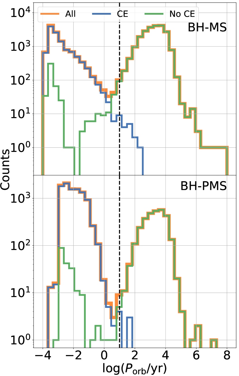
Figure 17: Same as Figure 1 but for the BH-LCs in our delayed model.

Figure 18 shows the relevant LC properties for the intrinsic population of BH-LC binaries in our delayed model.

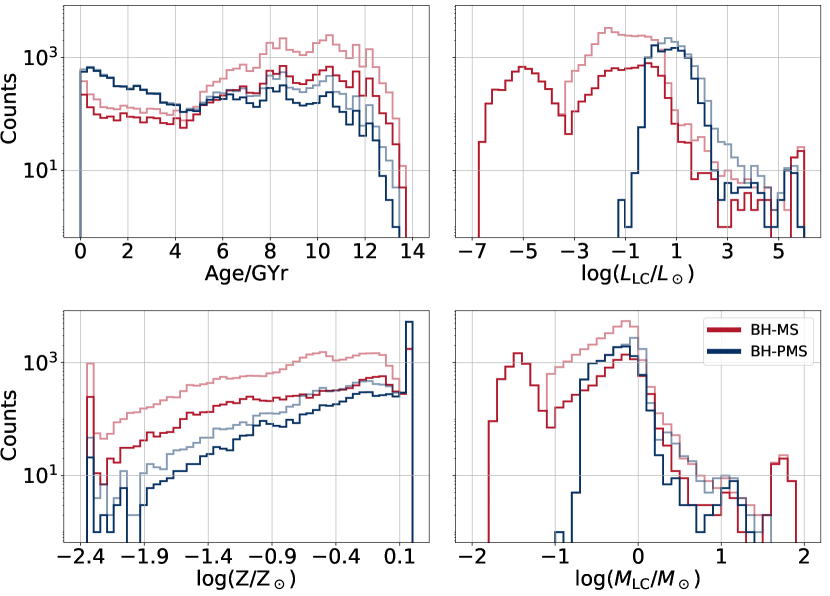
Figure 18: Same as Figure 4 except for the BH-LC binaries in our delayed model.

We have used propagation of error to estimate $\Delta{{M_{\rm{BH}}}}$ from the analytic expression for the astrometric mass function for the LC’s motion (without the $\sin i$ degeneracy) given in Equation 11. Andrews et al. (2019) derived this expression using a suite of Markov-chain Monete Carlo parameter-estimation exercise using injected LC motion as would be seen by Gaia assuming a $5$-${{\rm{yr}}}$ mission duration. We have updated their expression for a $10$-${{\rm{yr}}}$ Gaia mission for our purpose. Below we show the steps used to derive subsection 3.3 from Equation 11. For simplicity, we write the astrometric mass function without the $\sin\ i$ term as-

$$x \equiv \frac{{{M_{\rm{BH}}}}^{3}}{({{M_{\rm{BH}}}}+{{M_{\rm{LC}}}})^{2}}$$ (1)

$$= {{M_{\rm{BH}}}}\left(1+\frac{{{M_{\rm{LC}}}}}{{{M_{\rm{BH}}}}}\right)^{-2}$$

$$= {{M_{\rm{BH}}}}\times y^{-2},$$

where, we have used $y=(1+{{M_{\rm{LC}}}}/{{M_{\rm{BH}}}})$. Taking $\ln$ on both sides of Equation 1 and differentiating we get-

$$\frac{\partial x}{x}=\frac{\partial{{M_{\rm{BH}}}}}{{{M_{\rm{BH}}}}}-2\frac{\partial y}{y}$$ (2)

Since, $y$ is a function of both ${{M_{\rm{BH}}}}$ and ${{M_{\rm{LC}}}}$, we evaluate $\partial y/y$ as-

$$\frac{\partial y}{y} = \left.\frac{dy}{d{{M_{\rm{BH}}}}}\right|_{{{M_{\rm{LC}}}}}\frac{\partial{{M_{\rm{BH}}}}}{y}+\left.\frac{dy}{d{{M_{\rm{LC}}}}}\right|_{{{M_{\rm{BH}}}}}\frac{\partial{{M_{\rm{LC}}}}}{y}$$ (3)

$$= -\frac{2{{M_{\rm{LC}}}}}{{{M_{\rm{BH}}}}^{2}}\frac{\partial{{M_{\rm{BH}}}}}{y}+\frac{2}{{{M_{\rm{BH}}}}}\frac{\partial{{M_{\rm{LC}}}}}{y}.$$

Combining Equation 1, 2, and 3 we find,

$$\frac{\partial{{M_{\rm{BH}}}}}{{{M_{\rm{BH}}}}}=\frac{{M_{\rm{tot}}}}{{M_{\rm{tot}}}+2{{M_{\rm{LC}}}}}\frac{\partial x}{x}+\frac{2{{M_{\rm{LC}}}}}{{M_{\rm{tot}}}+2{{M_{\rm{LC}}}}}\frac{\partial{{M_{\rm{LC}}}}}{{{M_{\rm{LC}}}}}$$ (4)

Using Equation 4 and 11, replacing $x$, equating differentials with errors, and taking absolute values of possible errors, we find subsection 3.3.

References

- Abbott et al. (2016a) Abbott, B. P., Abbott, R., Abbott, T. D., et al. 2016a, Phys. Rev. Lett., 116, 1, doi: 10.1103/PhysRevLett.116.061102
- Abbott et al. (2016b) —. 2016b, Phys. Rev. Lett., 116, 1, doi: 10.1103/PhysRevLett.116.241103
- Abbott et al. (2019) —. 2019, Phys. Rev. X, 9, 031040, doi: 10.1103/PhysRevX.9.031040
- Abbott et al. (2021a) Abbott, R., Abbott, T. D., Abraham, S., et al. 2021a, Physical Review X, 11, 021053, doi: 10.1103/PhysRevX.11.021053
- Abbott et al. (2021b) —. 2021b, ApJ, 913, L7, doi: 10.3847/2041-8213/abe949
- Anders et al. (2019) Anders, F., Khalatyan, A., Chiappini, C., et al. 2019, VizieR Online Data Catalog, I/349
- Andrews et al. (2019) Andrews, J. J., Breivik, K., & Chatterjee, S. 2019, The Astrophysical Journal, 886, 68, doi: 10.3847/1538-4357/ab441f
- Astropy Collaboration et al. (2013) Astropy Collaboration, Robitaille, T. P., Tollerud, E. J., et al. 2013, A&A, 558, A33, doi: 10.1051/0004-6361/201322068
- Atri et al. (2019) Atri, P., Miller-Jones, J. C. A., Bahramian, A., et al. 2019, MNRAS, 489, 3116, doi: 10.1093/mnras/stz2335
- Barstow et al. (2014) Barstow, M. A., Casewell, S. L., Catalan, S., et al. 2014, arXiv e-prints, arXiv:1407.6163. https://arxiv.org/abs/1407.6163
- Bavera et al. (2021) Bavera, S. S., Fragos, T., Zevin, M., et al. 2021, A&A, 647, A153, doi: 10.1051/0004-6361/202039804
- Belczynski et al. (2010) Belczynski, K., Dominik, M., Bulik, T., et al. 2010, ApJ, 715, L138, doi: 10.1088/2041-8205/715/2/L138
- Belczynski et al. (2008) Belczynski, K., Kalogera, V., Rasio, F. A., et al. 2008, Astrophys. J. Suppl. Ser., 174, 223, doi: 10.1086/521026
- Biswas et al. (2021) Biswas, B., Nandi, R., Char, P., Bose, S., & Stergioulas, N. 2021, MNRAS, 505, 1600, doi: 10.1093/mnras/stab1383
- Boco et al. (2021) Boco, L., Lapi, A., Chruslinska, M., et al. 2021, ApJ, 907, 110, doi: 10.3847/1538-4357/abd3a0
- Bovy et al. (2016) Bovy, J., Rix, H.-W., Green, G. M., Schlafly, E. F., & Finkbeiner, D. P. 2016, The Astrophysical Journal, 818, 130, doi: 10.3847/0004-637x/818/2/130
- Brandt et al. (1995) Brandt, W. N., Podsiadlowski, P., & Sigurdsson, S. 1995, MNRAS, 277, L35, doi: 10.1093/mnras/277.1.L35
- Breivik et al. (2019) Breivik, K., Chatterjee, S., & Andrews, J. J. 2019, ApJ, 878, L4, doi: 10.3847/2041-8213/ab21d3
- Breivik et al. (2017) Breivik, K., Chatterjee, S., & Larson, S. L. 2017, The Astrophysical Journal, 850, L13, doi: 10.3847/2041-8213/aa97d5
- Breivik et al. (2020) Breivik, K., Coughlin, S., Zevin, M., et al. 2020, ApJ, 898, 71, doi: 10.3847/1538-4357/ab9d85
- Brogaard et al. (2018) Brogaard, K., Hansen, C. J., Miglio, A., et al. 2018, Mon. Not. R. Astron. Soc., 476, 3729, doi: 10.1093/MNRAS/STY268
- Brown & Bethe (1994) Brown, G. E., & Bethe, H. A. 1994, Astrophys. J., 423, doi: 10.1086/173844
- Chatterjee et al. (2017) Chatterjee, S., Rodriguez, C. L., Kalogera, V., & Rasio, F. A. 2017, ApJ, 836, L26, doi: 10.3847/2041-8213/aa5caa
- Chatterjee et al. (2017) Chatterjee, S., Rodriguez, C. L., & Rasio, F. A. 2017, Astrophys. J., 834, 68, doi: 10.3847/1538-4357/834/1/68
- Chatziioannou et al. (2017) Chatziioannou, K., Clark, J. A., Bauswein, A., et al. 2017, Phys. Rev. D, 96, 124035, doi: 10.1103/PhysRevD.96.124035
- Chawla et al. (2021) Chawla, C., Chatterjee, S., Breivik, K., et al. 2021, Gaia May Detect Hundreds of Well-characterised Stellar Black Holes, Zenodo, doi: 10.5281/zenodo.5993252. https://doi.org/10.5281/zenodo.5993252
- Claeys et al. (2014) Claeys, J. S. W., Pols, O. R., Izzard, R. G., Vink, J., & Verbunt, F. W. M. 2014, A&A, 563, A83, doi: 10.1051/0004-6361/201322714
- Corral-Santana et al. (2016) Corral-Santana, J. M., Casares, J., Muñoz-Darias, T., et al. 2016, Astron. Astrophys., 587, doi: 10.1051/0004-6361/201527130
- Cromartie et al. (2020) Cromartie, H. T., Fonseca, E., Ransom, S. M., et al. 2020, Nature Astronomy, 4, 72, doi: 10.1038/s41550-019-0880-2
- Davis et al. (2005) Davis, S. W., Blaes, O. M., Hubeny, I., & Turner, N. J. 2005, ApJ, 621, 372, doi: 10.1086/427278
- Drimmel et al. (2003) Drimmel, R., Cabrera-Lavers, A., & López-Corredoira, M. 2003, Astron. Astrophys., 409, 205, doi: 10.1051/0004-6361:20031070
- Fabbiano (2012) Fabbiano, G. 2012, Accretion Process. Astrophys. XXI Canar. Islands Winter Sch. Astrophys., 9781107030190, 151, doi: 10.1017/CBO9781139343268.006
- Fishbach & Holz (2017) Fishbach, M., & Holz, D. E. 2017, ApJ, 851, L25, doi: 10.3847/2041-8213/aa9bf6
- Fragos et al. (2009) Fragos, T., Willems, B., Kalogera, V., et al. 2009, ApJ, 697, 1057, doi: 10.1088/0004-637X/697/2/1057
- Frank et al. (2002) Frank, J., King, A., & Raine, D. J. 2002, Accretion Power in Astrophysics: Third Edition
- Fryer et al. (2012) Fryer, C. L., Belczynski, K., Wiktorowicz, G., et al. 2012, Astrophys. J., 749, doi: 10.1088/0004-637X/749/1/91
- Gallenne et al. (2016) Gallenne, A., Pietrzyński, G., Graczyk, D., et al. 2016, Astron. Astrophys., 586, 1, doi: 10.1051/0004-6361/201526764
- Gallo et al. (2014) Gallo, E., Miller-Jones, J. C., Russell, D. M., et al. 2014, Mon. Not. R. Astron. Soc., 445, 290, doi: 10.1093/mnras/stu1599
- Gandhi et al. (2020) Gandhi, P., Buckley, D. A. H., Charles, P., et al. 2020, 8, 1
- Giesers et al. (2018) Giesers, B., Dreizler, S., Husser, T. O., et al. 2018, Mon. Not. R. Astron. Soc. Lett., 475, L15, doi: 10.1093/mnrasl/slx203
- Giesers et al. (2019) Giesers, B., Kamann, S., Dreizler, S., et al. 2019, A&A, 632, A3, doi: 10.1051/0004-6361/201936203
- Goldberg & Mazeh (1994) Goldberg, D., & Mazeh, T. 1994, A&A, 282, 801
- Gould & Salim (2002) Gould, A., & Salim, S. 2002, ApJ, 572, 944, doi: 10.1086/340435
- Green et al. (2019) Green, G. M., Schlafly, E., Zucker, C., Speagle, J. S., & Finkbeiner, D. 2019, The Astrophysical Journal, 887, 93, doi: 10.3847/1538-4357/ab5362
- Gualandris et al. (2005) Gualandris, A., Colpi, M., Portegies Zwart, S., & Possenti, A. 2005, ApJ, 618, 845, doi: 10.1086/426126
- Güver & Özel (2009) Güver, T., & Özel, F. 2009, Mon. Not. R. Astron. Soc., 400, 2050, doi: 10.1111/j.1365-2966.2009.15598.x
- Han (1998) Han, Z. 1998, MNRAS, 296, 1019, doi: 10.1046/j.1365-8711.1998.01475.x
- Heggie (1975) Heggie, D. C. 1975, Mon. Not. R. Astron. Soc., 173, doi: 10.1093/mnras/173.3.729
- Hobbs et al. (2005) Hobbs, G., Lorimer, D. R., Lyne, A. G., & Kramer, M. 2005, Mon. Not. R. Astron. Soc., 360, doi: 10.1111/j.1365-2966.2005.09087.x
- Hopkins et al. (2018) Hopkins, P. F., Wetzel, A., Kereš, D., et al. 2018, MNRAS, 480, 800, doi: 10.1093/mnras/sty1690
- Howes et al. (2019) Howes, L. M., Lindegren, L., Feltzing, S., Church, R. P., & Bensby, T. 2019, A&A, 622, A27, doi: 10.1051/0004-6361/201833280
- Hunter (2007) Hunter, J. D. 2007, Computing in Science and Engineering, 9, 90, doi: 10.1109/MCSE.2007.55
- Hurley et al. (2000) Hurley, J. R., Pols, O. R., & Tout, C. A. 2000, MNRAS, 315, 543, doi: 10.1046/j.1365-8711.2000.03426.x
- Hurley et al. (2002) Hurley, J. R., Tout, C. A., & Pols, O. R. 2002, Mon. Not. R. Astron. Soc., 329, doi: 10.1046/j.1365-8711.2002.05038.x
- Ivanova & Taam (2004) Ivanova, N., & Taam, R. E. 2004, ApJ, 601, 1058, doi: 10.1086/380561
- Jayasinghe et al. (2021) Jayasinghe, T., Stanek, K. Z., Thompson, T. A., et al. 2021, MNRAS, 504, 2577, doi: 10.1093/mnras/stab907
- Jones et al. (2001) Jones, E., Oliphant, T., Peterson, P., et al. 2001, SciPy: Open source scientific tools for Python. http://www.scipy.org/
- Jonker et al. (2021) Jonker, P. G., Kaur, K., Stone, N., & Torres, M. A. P. 2021, arXiv e-prints, arXiv:2104.03596. https://arxiv.org/abs/2104.03596
- Knuth (2019) Knuth, K. H. 2019, Digital Signal Processing, 95, 102581, doi: https://doi.org/10.1016/j.dsp.2019.102581
- Kollmeier et al. (2019) Kollmeier, J., Anderson, S. F., Blanc, G. A., et al. 2019, in Bulletin of the American Astronomical Society, Vol. 51, 274
- Kreidberg et al. (2012) Kreidberg, L., Bailyn, C. D., Farr, W. M., & Kalogera, V. 2012, ApJ, 757, 36, doi: 10.1088/0004-637X/757/1/36
- Kremer et al. (2018) Kremer, K., Chatterjee, S., Rodriguez, C. L., & Rasio, F. A. 2018, arXiv e-prints, arXiv:1802.04895. https://arxiv.org/abs/1802.04895
- Kroupa (2001) Kroupa, P. 2001, Mon. Not. R. Astron. Soc., 322, doi: 10.1046/j.1365-8711.2001.04022.x
- Kruckow et al. (2016) Kruckow, M. U., Tauris, T. M., Langer, N., et al. 2016, A&A, 596, A58, doi: 10.1051/0004-6361/201629420
- Lindegren et al. (2012) Lindegren, L., Lammers, U., Hobbs, D., et al. 2012, Astron. Astrophys., 538, doi: 10.1051/0004-6361/201117905
- Lindegren et al. (2018) Lindegren, L., Hernández, J., Bombrun, A., et al. 2018, Astron. Astrophys., 616, doi: 10.1051/0004-6361/201832727
- Livio & Soker (1984) Livio, M., & Soker, N. 1984, MNRAS, 208, 763, doi: 10.1093/mnras/208.4.763
- Marshall et al. (2006) Marshall, D. J., Robin, A. C., Reylé, C., Schultheis, M., & Picaud, S. 2006, Astron. Astrophys., 453, 635, doi: 10.1051/0004-6361:20053842
- Mashian & Loeb (2017) Mashian, N., & Loeb, A. 2017, Mon. Not. R. Astron. Soc., 470, doi: 10.1093/mnras/stx1410
- Mazeh et al. (1992) Mazeh, T., Goldberg, D., Duquennoy, A., & Mayor, M. 1992, ApJ, 401, 265, doi: 10.1086/172058
- Merloni et al. (2012) Merloni, A., Predehl, P., Becker, W., et al. 2012. https://arxiv.org/abs/1209.3114
- Milone et al. (2020) Milone, A. P., Marino, A. F., Da Costa, G. S., et al. 2020, MNRAS, 491, 515, doi: 10.1093/mnras/stz2999
- Morton (2015) Morton, T. D. 2015, isochrones: Stellar model grid package. http://ascl.net/1503.010
- Olejak, A. et al. (2020) Olejak, A., Belczynski, K., Bulik, T., & Sobolewska, M. 2020, A&A, 638, A94, doi: 10.1051/0004-6361/201936557
- Paczynski (1976) Paczynski, B. 1976, in Structure and Evolution of Close Binary Systems, ed. P. Eggleton, S. Mitton, & J. Whelan, Vol. 73, 75
- Pavlovski et al. (2018) Pavlovski, K., Southworth, J., & Tamajo, E. 2018, Mon. Not. R. Astron. Soc., 481, 3129, doi: 10.1093/mnras/sty2516
- Pejcha (2020) Pejcha, O. 2020, Rev. Front. Mod. Astrophys., 189, doi: 10.1007/978-3-030-38509-5_7
- Price-Whelan et al. (2018) Price-Whelan, A. M., Sipőcz, B. M., Günther, H. M., et al. 2018, AJ, 156, 123, doi: 10.3847/1538-3881/aabc4f
- Price-Whelan et al. (2020) Price-Whelan, A. M., Hogg, D. W., Rix, H.-W., et al. 2020, Astrophys. J., 895, 2, doi: 10.3847/1538-4357/ab8acc
- Remillard & McClintock (2006) Remillard, R. A., & McClintock, J. E. 2006, Annu. Rev. Astron. Astrophys., 44, 49, doi: 10.1146/annurev.astro.44.051905.092532
- Rendle et al. (2019) Rendle, B. M., Buldgen, G., Miglio, A., et al. 2019, MNRAS, 484, 771, doi: 10.1093/mnras/stz031
- Repetto et al. (2012) Repetto, S., Davies, M. B., & Sigurdsson, S. 2012, MNRAS, 425, 2799, doi: 10.1111/j.1365-2966.2012.21549.x
- Repetto & Nelemans (2015) Repetto, S., & Nelemans, G. 2015, MNRAS, 453, 3341, doi: 10.1093/mnras/stv1753
- Rodriguez et al. (2021) Rodriguez, C. L., Weatherford, N. C., Coughlin, S. C., et al. 2021, arXiv e-prints, arXiv:2106.02643. https://arxiv.org/abs/2106.02643
- Samland (1998) Samland, M. 1998, Astrophys. J., 496, 155, doi: 10.1086/305368
- Sanderson et al. (2020) Sanderson, R. E., Wetzel, A., Loebman, S., et al. 2020, Astrophys. J. Suppl. Ser., 246, doi: 10.3847/1538-4365/ab5b9d
- Shikauchi et al. (2020) Shikauchi, M., Kumamoto, J., Tanikawa, A., & Fujii, M. S. 2020, PASJ, 72, 45, doi: 10.1093/pasj/psaa030
- Sukhbold et al. (2016) Sukhbold, T., Ertl, T., Woosley, S. E., Brown, J. M., & Janka, H.-T. 2016, Core-Collapse Supernovae From 9 To 120 Solar Masses Based on Neutrino-Powered Explosions, IOP Publishing, doi: 10.3847/0004-637x/821/1/38. http://dx.doi.org/10.3847/0004-637X/821/1/38
- Sukhbold et al. (2018) Sukhbold, T., Woosley, S. E., & Heger, A. 2018, ApJ, 860, 93, doi: 10.3847/1538-4357/aac2da
- Tetarenko et al. (2016) Tetarenko, B. E., Sivakoff, G. R., Heinke, C. O., & Gladstone, J. C. 2016, Astrophys. J. Suppl. Ser., 222, 15, doi: 10.3847/0067-0049/222/2/15
- Thompson et al. (2019) Thompson, T. A., Kochanek, C. S., Stanek, K. Z., et al. 2019, Science (80-. )., 366, 637, doi: 10.1126/science.aau4005
- Timmes et al. (1996) Timmes, F. X., Woosley, S. E., & Weaver, T. A. 1996, Astrophys. J., 457, 834, doi: 10.1086/176778
- Torres & Ribas (2002) Torres, G., & Ribas, I. 2002, Astrophys. J., 567, 1140, doi: 10.1086/338587
- Tout et al. (1997) Tout, C. A., Aarseth, S. J., Pols, O. R., & Eggleton, P. P. 1997, MNRAS, 291, 732, doi: 10.1093/mnras/291.4.732
- van der Walt et al. (2011) van der Walt, S., Colbert, S. C., & Varoquaux, G. 2011, Computing in Science and Engineering, 13, 22, doi: 10.1109/MCSE.2011.37
- Weisskopf et al. (2000) Weisskopf, M. C., Tananbaum, H. D., Speybroeck, L. P. V., & O’Dell, S. L. 2000, in X-Ray Optics, Instruments, and Missions III, ed. J. E. Truemper & B. Aschenbach, Vol. 4012, International Society for Optics and Photonics (SPIE), 2 – 16. https://doi.org/10.1117/12.391545
- Wetzel et al. (2016) Wetzel, A. R., Hopkins, P. F., Kim, J.-h., et al. 2016, Astrophys. J., 827, L23, doi: 10.3847/2041-8205/827/2/l23
- Wiktorowicz et al. (2020) Wiktorowicz, G., Lu, Y., Wyrzykowski, Ł., et al. 2020, The Astrophysical Journal, 905, 134, doi: 10.3847/1538-4357/abc699
- Wilms et al. (2000) Wilms, J., Allen, A., & McCray, R. 2000, The Astrophysical Journal, 542, 914, doi: 10.1086/317016
- Wong et al. (2014) Wong, T.-W., Valsecchi, F., Ansari, A., et al. 2014, ApJ, 790, 119, doi: 10.1088/0004-637X/790/2/119
- Woosley (2017) Woosley, S. E. 2017, Astrophys. J., 836, 244, doi: 10.3847/1538-4357/836/2/244
- Woosley et al. (2002) Woosley, S. E., Heger, A., & Weaver, T. A. 2002, Reviews of Modern Physics, 74, 1015, doi: 10.1103/RevModPhys.74.1015
- Wyrzykowski & Mandel (2020) Wyrzykowski, Ł., & Mandel, I. 2020, A&A, 636, A20, doi: 10.1051/0004-6361/201935842
- Xie & Yuan (2012) Xie, F. G., & Yuan, F. 2012, Mon. Not. R. Astron. Soc., 427, 1580, doi: 10.1111/j.1365-2966.2012.22030.x
- Yalinewich et al. (2018) Yalinewich, A., Beniamini, P., Hotokezaka, K., & Zhu, W. 2018, Mon. Not. R. Astron. Soc., 481, 930, doi: 10.1093/mnras/sty2327
- Yamaguchi et al. (2018) Yamaguchi, M. S., Kawanaka, N., Bulik, T., & Piran, T. 2018, The Astrophysical Journal, 861, 21, doi: 10.3847/1538-4357/aac5ec
- Yang et al. (2015) Yang, Q. X., Xie, F. G., Yuan, F., et al. 2015, Mon. Not. R. Astron. Soc., 447, 1692, doi: 10.1093/mnras/stu2571
- Zasowski et al. (2013) Zasowski, G., Johnson, J. A., Frinchaboy, P. M., et al. 2013, Astron. J., 146, doi: 10.1088/0004-6256/146/4/81
- Zasowski et al. (2017) Zasowski, G., Cohen, R. E., Chojnowski, S. D., et al. 2017, AJ, 154, 198, doi: 10.3847/1538-3881/aa8df9