HyperCube: Implicit Field Representations of Voxelized 3D Models

Abstract

Recently introduced implicit field representations offer an effective way of generating 3D object shapes. They leverage implicit decoder trained to take a 3D point coordinate concatenated with a shape encoding and to output a value which indicates whether the point is outside the shape or not. Although this approach enables efficient rendering of visually plausible objects, it has two significant limitations. First, it is based on a single neural network dedicated for all objects from a training set which results in a cumbersome training procedure and its application in real life. More importantly, the implicit decoder takes only points sampled within voxels (and not the entire voxels) which yields problems at the classification boundaries and results in empty spaces within the rendered mesh.

To solve the above limitations, we introduce a new HyperCube architecture based on interval arithmetic network, that enables direct processing of 3D voxels, trained using a hypernetwork paradigm to enforce model convergence. Instead of processing individual 3D samples from within a voxel, our approach allows to input the entire voxel (3D cube) represented with its convex hull coordinates, while the target network constructed by a hypernet assigns it to an inside or outside category. As a result our HyperCube model outperforms the competing approaches both in terms of training and inference efficiency, as well as the final mesh quality.

1 Introduction

Recently introduced implicit field representations of 3D objects offer high quality generations of 3D shapes [1]. This method relies on an implicit decoder, called IM-NET, trained to take a 3D point coordinate concatenated with a shape encoding and to assign it a value indicating whether it belongs inside or outside of a given shape. Using this formulation, a shape is constructed out of points assigned to the inside class and it is typically rendered via the iso-surface extraction method such as Marching Cubes.

input
IM-NET
HyperCube

Figure 1: Comparison between our HyperCube approach and the state-of-the-art implicit field method based on the IM-NET [1]. IM-NET takes as an input 3D points sampled within voxels, while HyperCube leverages an interval arithmetic to process the entire voxels. As a result, HyperCube offers a high quality 3D object rendering without missing important parts of object close to the implicit decoder’s decision boundary, as done by IM-NET.

The IM-NET architecture has several advantages over a standard convolutional model. First of all, it can produce outputs of various resolutions, including those not observed in the training. Furthermore, IM-NET learns shape boundaries instead of voxel distributions over the volume, which results in surfaces of a higher quality.

On the other hand, however, IM-NET has some limitations. First of all, the point coordinates processed by the model are concatenated with the shape embedding and to reconstruct an object the model needs to possess the knowledge about all objects present in the entire dataset. Therefore IM-NET architecture is hard to train on many different classes. Moreover, the implicit decoder processes only points sampled from within a voxel, instead of the entire voxels. This, in turn, yields problems at the classification boundaries at object edges and gives severe rendering artifacts, see Fig. 1.

In this paper, we address the above limitations by introducing a novel approach to 3D object representation based on implicit fields called HyperCube. Contrary to the baseline IM-NET model, our approach leverages a hyper-network architecture to produce weights of a target implicit decoder, based on the input feature vector defining a voxel. This target decoder assigns an inside or outside of a shape label to each processed voxel. Such architecture is more compact than IM-NET and therefore much faster to train, while it does not need to know the distribution of all objects in the training dataset to obtain object reconstructions. Furthermore, its design allows a flexible adjustment of the target network processing feature vectors. This enables us to input the entire voxels into the model leveraging interval arithmetic and the IntervalNet architecture [2, 3] and leading to the inception of our HyperFlow model. The HyperFlow architecture takes as an input relatively small 3D cubes (hence the name), instead of 3D points samples within the voxels. Therefore, it does not produce empty space in reconstructed mesh representation, as done by the IM-NET and visualized in Fig. 1.

To summarize, our contributions are the following:

• We introduce a new HyperCube architecture for representing voxelized 3D models based on implicit field representation.

• We incorporate a hypernetwork paradigm into our architecture which leads to significant simplification of the resulting model and reduces training time.

• Our approach offers unprecedented flexibility of integrating various target network models, and we show on the example of the IntervalNet how this can be leveraged to work with the entire voxels, and not their sampled versions, which significantly improves the quality of generated 3D models.

2 Related works

3D objects can be represented using different approaches including voxel grids [4, 5, 6, 7], octrees [8, 9, 10, 11], multi-view images [12, 13, 14], point clouds [15, 16, 17, 18, 19], geometry images [20, 21], deformable meshes [5, 21, 22, 19], and part-based structural graphs [23, 24].

All the above representations are discreet which hinders their application in real-life scenarios. Therefore recent works introduced 3D representations modeled as a continuous function [25]. In such a case the implicit occupancy [1, 26, 27], distance field [28, 29] and surface parametrization [30, 31, 32, 33] models use a neural network to represent a 3D object. These methods do not use discretization (e.g., fixed number of voxels, points, or vertices), but represent shapes in a continuous manner and handle complicated shape topologies.

In [26] the authors propose that the occupancy networks implicitly represent the 3D surface as a continuous decision boundary of a deep neural network classifier. Thus, the occupancy networks produce continuous representation instead of a discrete one, and render realistic high-resolution meshes. In [1], which is the most relevant baseline to our approach, the authors propose an implicit decoder (IM-NET). Such a model uses a binary classifier that takes a point coordinate concatenated with a feature vector encoding a shape and outputs a value that indicates inside or outside label. The above-mentioned implicit approaches are limited to rather simple geometries of single objects and do not scale to more complicated or large-scale scenes. In [27], the authors propose Convolutional Occupancy Networks, dedicated for the representations of 3D scenes. The authors use convolutional encoders and implicit decoders. In general, all above method uses conditioning mechanism. In our paper, we use the hyper network, which gives a more flexible model which can be trained faster.

In [29] the authors introduce DeepSDF representation of 3D objects that produce high-quality meshes. DeepSDF represents a shape surface by a continuous volumetric field. Points represent the distance to the surface boundary, and the sign indicates whether the region is inside or outside. Such representation implicitly encodes a shape’s border as a classification boundary.

In [31, 32] the authors propose HyperCloud model that uses a hyper network to output weights of a generative network to create 3D point clouds, instead of generating a fixed size reconstruction. One neural network is trained to produce a continuous representation of an object. In [30] authors propose to use a conditioning mechanism to produce a flow model which transfers gaussian noise into a 3D object.

Our solution can be interpreted as a generalization of all the above methods. We use data reprehension approach described in IM-NET, but extend it to follow the hypernetwork paradigm used in HyperCloud. As a consequence, we take the best of both wordls and obtain a reconstruction quality of the IM-NET, while reducing the training and inference time as in the case of a HyperCloud.

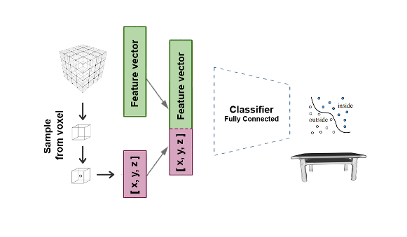
(a) IM-NET

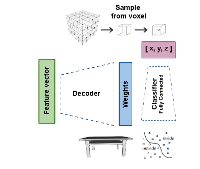
(b) HyperCube

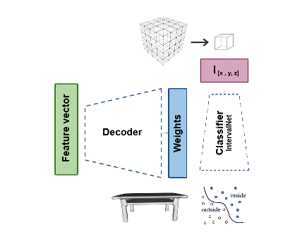
(c) HyperFlow

​ ​ ​

Figure 2: Comparison of the network architectures: (a) IM-NET, (b) HyperCube and (c) HyperFlow. (a) IM-NET uses a binary classifier that takes a point coordinate $(x,y,z)$ concatenated with a feature vector encoding a shape and outputs a value which indicates whether the point is outside the shape or not. IM-NET is a single neural network dedicated to all object from the training dataset. (b) HyperCube takes feature vectors and produce a new network, dubbed target network which classifies points sampled from voxel into one of two categories: inside or outside. For object reconstruction, only a target network run on a 3D cube is needed, which makes this solution significantly faster. (c) HyperFlow extends HyperCube idea by incorporating interval arithmetic which in turn allows to process the entire voxel by an IntervalNet, instead of samples of voxels, as done in the IM-NET.

3 Hyper Implicit Field

In this section, we present the HyperCube model designed to produce a continuous representation of Implicit Fields. More precisely, for each 3D object represented by voxels, we would like to create a neural network that classifies elements from $\mathbb{R}^{3}$ to the inside or outside classes. We define voxel representation as a unit cube $[0,1]\times[0,1]\times[0,1]$ divided into small cubes with a given resolution $n\in\mathbb{N}$:

$$V_{n}=\left\{[\stackunder[1.2pt]{$x$}{\rule{3.44444pt}{0.32289pt}}_{i},\bar{x}_{i}]\times[\stackunder[1.2pt]{$y$}{\rule{3.44444pt}{0.32289pt}}_{i},\bar{y}_{i}]\times[\stackunder[1.2pt]{$z$}{\rule{3.44444pt}{0.32289pt}}_{i},\bar{z}_{i}]\mbox{ where }\stackunder[1.2pt]{$x$}{\rule{3.44444pt}{0.32289pt}}_{i},\stackunder[1.2pt]{$y$}{\rule{3.44444pt}{0.32289pt}}_{i},\stackunder[1.2pt]{$z$}{\rule{3.44444pt}{0.32289pt}}_{i}=0,\frac{1}{n},\frac{2}{n},\ldots,\frac{n-1}{n}\right.\\ \left.\mbox{ and }\bar{x}_{i}=\stackunder[1.2pt]{$x$}{\rule{3.44444pt}{0.32289pt}}_{i}+\frac{1}{n},\bar{y}_{i}=\stackunder[1.2pt]{$y$}{\rule{3.44444pt}{0.32289pt}}_{i}+\frac{1}{n},\bar{z}_{i}=\stackunder[1.2pt]{$z$}{\rule{3.44444pt}{0.32289pt}}_{i}+\frac{1}{n}\right\}.$$

During the training, we use binary labels for each element of the voxel grid: $\mathcal{X}=\left\{I_{i}\right\}_{i=1}^{n^{3}},y\subset\{0,1\}^{n^{3}},$ where $I_{i}=[\stackunder[1.2pt]{$x$}{\rule{3.44444pt}{0.32289pt}}_{i},\bar{x}_{i}]\times[\stackunder[1.2pt]{$y$}{\rule{3.44444pt}{0.32289pt}}_{i},\bar{y}_{i}]\times[\stackunder[1.2pt]{$z$}{\rule{3.44444pt}{0.32289pt}}_{i},\bar{z}_{i}]\in V_{n}$. Although the labels are assigned to the voxels defined as 3D cubes, a classical neural networks are not able to process them in the raw continuous format. Therefore, such methods use points uniformly sampled from a voxel: $X=\left\{(x_{i},y_{i},z_{i}):(x_{i},y_{i},z_{i})\sim\mathcal{U}_{I_{i}}\right\}_{i=1}^{n^{3}},y\subset\{0,1\}^{n^{3}},$ where $\mathcal{U}_{I_{i}}$ is uniform distribution in 3D cube $I_{i}$. In the paper, we present a method that works directly with voxels.

We assume that we have feature vectors for each element from the training set. Our goal is to build a continuous representation of 3D objects. More precisely we have to model function $f\colon\mathbb{R}^{3}\to\{0,1\}$, which takes coordinate of 3D point and returns an inside/outside label. Reconstruction of the object is produced by labeling all elements from the voxel grid using the Marching Cubes algorithm.

In this section, we first describe a general hyper network architecture used in our model. We follow up with the description of our HyperCube method, which uses hyper networks to efficiently process 3D points. Finally, we introduce interval arithmetic, which allows us to propagate 3D cubes instead of point sampled from voxels, and we show how we can use incorporate is within our approach HyperFlow.

3.1 Hypernetwork

Hyper networks, introduced in [34], are defined as neural models that generate weights for target network solving a specific task. The authors aim to reduce trainable parameters by designing a hyper-network with a smaller number of parameters than the target network.

In the context of 3D point clouds, various methods make use of a hyper network to produce a continuous representation of objects [31, 35, 36]. HyperCloud [31] proposes a generative autoencoder-based model that relies on a decoder to produce a vector of weights $\theta$ of a target network $\mathcal{T}_{\theta}\colon\mathbb{R}^{3}\to\mathbb{R}^{3}$. The target network is designed to transform a prior into target objects (reconstructed data). In practice, we have one neural network architecture that uses different weights for each 3D object.

HyperCube
HyperCube
HyperCube
HyperCube
HyperCube

Figure 3: Interpolations produce by HyperCube. We take two 3d objects and obtain a smooth transition between them.

3.2 HyperCube

In this section, we introduce our HyperCube approach that draws the inspiration from the above methods to address the limitations of the baseline IM-NET model. We produce weights for a target network that describes a 3D object. Instead of transferring a prior distribution, as done in the HyperCloud, we transfer through a network a voxel grid to predict inside/outside label for each coordinate, see Fig. 2(b).

HyperCube model uses a hyper network to output weights of a small neural network that creates a 3D voxel representation of a 3D object, instead of generating a directly inside/outside label to a fixed grid on a 3D cube. More specifically, we parametrize the surface of 3D objects as a function $f:\mathbb{R}^{3}\to\{0,1\}$, which returns ab inside/outside category, given a point from grid $(x,y,z)$. In other words, instead of producing a 3D voxel representation, we construct a model which create multiple neural networks (a different neural network for each object) that model the surfaces of the objects.

In practice, we have one large architecture (hyper network) that produces different weights for each 3D object (target network). More precisely, we model function $T_{\theta}:\mathbb{R}^{3}\to\mathbb{R}$ (neural network classifier with weights $\theta$), which takes an element from the voxel grid and predicts an inside/outside label. In consequence, we can generate a 3D shape at any resolution by creating grids of different sizes and predict labels for its voxels.

The target network is not trained directly. We use a hyper-network $\begin{array}[]{c}H_{\phi}:\mathbb{R}^{3}\supset X\to\theta,\end{array}$ which for a voxel representation returns weights $\theta$ to the corresponding target network $T_{\theta}:X\to\{0,1\}$. Thus, a 3D object is represented by a function (classifier)

$$\begin{array}[]{c}T((x,y,x);\theta)=T((x,y,x);H_{\phi}(X)).\end{array}$$

More precisely, we take a voxel representation $X$ and pass it to $H_{\phi}$. The hyper network returns weights $\theta$ to target network $T_{\theta}$. Next, the input voxel representation $X$ (points sampled from $\mathcal{X}$) is compared with the output from the target network $T_{\theta}$ (we take voxel grid and predict inside/outside labels). To train our model we use mean squared error loss function.

We train a single neural model (hypernetwork), which allows us to produce a variety of functions at test time. By interpolating in the space of hypernetwork parameters, we are able to produce multiple shapes that bear similarity to each other, as Fig. 3 shows.

The above architecture gives competitive qualitative and quantitative results to IM-NET, as we show in Section 4.2, yet it offers a significant processing speedup confirmed by the results presented in Section 4.1. However, the remaining shortcoming of IM-NET, namely the reconstruction artifacts close to classification boundaries resulting from sampling strategy, remains. To address this limitation and process entire 3D cubes instead of sampled points, we leverage interval arithmetic [37] and a neural architecture that implements it, IntervalNet [2, 3].

3.3 Interval arithmetic

Interval arithmetic allows to address the problems with precise numerical calculations caused by the rounding errors that appear within the computer representations of real numbers. In neural networks interval arithmetic is used to train models on interval data [38, 39, 40] and produce neural networks that are robust against adversarial attacks [2, 3].

For the convenience of the reader, we give a short description of interval arithmetic. Interval arithmetic [37](Chapter 2.5.3) is based on the operations on segments. Let us assume $A$ and $B$ as numbers expressed as interval. For all $\bar{a},\stackunder[1.2pt]{$a$}{\rule{3.44444pt}{0.32289pt}},\bar{b},\stackunder[1.2pt]{$b$}{\rule{3.44444pt}{0.32289pt}}\in R$ where $A=[\stackunder[1.2pt]{$a$}{\rule{3.44444pt}{0.32289pt}},\bar{a}]$ , $B=[\stackunder[1.2pt]{$b$}{\rule{3.44444pt}{0.32289pt}},\bar{b}]$, the main operations of intervals may be written as [41]:

• addition: $[\stackunder[1.2pt]{$a$}{\rule{3.44444pt}{0.32289pt}},\bar{a}]+[\stackunder[1.2pt]{$b$}{\rule{3.44444pt}{0.32289pt}},\bar{b}]=[\stackunder[1.2pt]{$a$}{\rule{3.44444pt}{0.32289pt}}+\stackunder[1.2pt]{$b$}{\rule{3.44444pt}{0.32289pt}},\bar{a}+\bar{b}]$

• subtraction: $[\stackunder[1.2pt]{$a$}{\rule{3.44444pt}{0.32289pt}},\bar{a}]-[\stackunder[1.2pt]{$b$}{\rule{3.44444pt}{0.32289pt}},\bar{b}]=[\stackunder[1.2pt]{$a$}{\rule{3.44444pt}{0.32289pt}}-\stackunder[1.2pt]{$b$}{\rule{3.44444pt}{0.32289pt}},\bar{a}-\bar{b}]$

• multiplication: $[\stackunder[1.2pt]{$a$}{\rule{3.44444pt}{0.32289pt}},\bar{a}]*[\stackunder[1.2pt]{$b$}{\rule{3.44444pt}{0.32289pt}},\bar{b}]=[\min(\stackunder[1.2pt]{$a$}{\rule{3.44444pt}{0.32289pt}}*\stackunder[1.2pt]{$b$}{\rule{3.44444pt}{0.32289pt}},\stackunder[1.2pt]{$a$}{\rule{3.44444pt}{0.32289pt}}*\bar{b},\bar{a}*\stackunder[1.2pt]{$b$}{\rule{3.44444pt}{0.32289pt}},\bar{a}*\bar{b}),\max(\stackunder[1.2pt]{$a$}{\rule{3.44444pt}{0.32289pt}}*\stackunder[1.2pt]{$b$}{\rule{3.44444pt}{0.32289pt}},\stackunder[1.2pt]{$a$}{\rule{3.44444pt}{0.32289pt}}*\bar{b},\bar{a}*\stackunder[1.2pt]{$b$}{\rule{3.44444pt}{0.32289pt}},\bar{a}*\bar{b})]$

• division: $[\stackunder[1.2pt]{$a$}{\rule{3.44444pt}{0.32289pt}},\bar{a}]\div[\stackunder[1.2pt]{$b$}{\rule{3.44444pt}{0.32289pt}},\bar{b}]=[\min(\stackunder[1.2pt]{$a$}{\rule{3.44444pt}{0.32289pt}}\div\stackunder[1.2pt]{$b$}{\rule{3.44444pt}{0.32289pt}},\stackunder[1.2pt]{$a$}{\rule{3.44444pt}{0.32289pt}}\div\bar{b},\bar{a}\div\stackunder[1.2pt]{$b$}{\rule{3.44444pt}{0.32289pt}},\bar{a}\div\bar{b}),\max(\stackunder[1.2pt]{$a$}{\rule{3.44444pt}{0.32289pt}}\div\stackunder[1.2pt]{$b$}{\rule{3.44444pt}{0.32289pt}},\stackunder[1.2pt]{$a$}{\rule{3.44444pt}{0.32289pt}}\div\bar{b},\bar{a}\div\stackunder[1.2pt]{$b$}{\rule{3.44444pt}{0.32289pt}},\bar{a}\div\bar{b})]$ excluding the case $\stackunder[1.2pt]{$b$}{\rule{3.44444pt}{0.32289pt}}=0$ or $\bar{b}=0$.

The above operations allow the construction of a neural network, which uses intervals instead of points on neural networks input. The following subsection shows that we can substitute classical arithmetic on points to the arithmetic on intervals and, consequently, directly work on voxels.

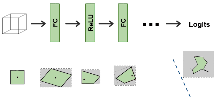
Figure 4: Illustration of IntervalNet 3D interval (illustrated in 2D for clarity) is propagated through MLP. At each layer, the 3D cube is deformed by linear transformation (FC layer). Then we construct interval bound (marked by gray color) and use the ReLU activation function. Interval bound (in gray) is propagated to the next layer. In logit space, it becomes easy to compute an upper bound on the worstcase violation. Interval bound (in gray) is moved on one side of the decision boundary and consequently transformed 3D cube (in green) is correctly classified. The figure is inspired by Fig. 2 from [2].

3.4 HyperFlow

Thanks to the interval arithmetic, we can construct IntervalNet [2, 3] that is able to process 3D cubes defined as intervals in the 3D space. Let us consider the feed-forward neural network trained for a classification task. We assume that the network is defined by a sequence of transformations $h_{k}$ for each of its $K$ layers. That is, for input $z_{0}$, we have

$$z_{k}=h_{k}(z_{k-1})\mbox{ for }k=1,\ldots,K.$$

The output $z_{K}\in\mathbb{R}^{N}$ has $N$ logits corresponding to $N$ classes. In the IntervalNet each transformation $h_{k}$ uses interval arithmetic. More precisely, the input of a layer is a 3D interval (3D cube).

Let us consider a classical dense layer:

$$h(x)=Wx+b.$$

In IntervalNet, the input of the network is an interval and consequently the output of a dense layer is also a vector of intervals:

$$[\stackunder[1.2pt]{h}{\rule{3.44444pt}{0.32289pt}}(x),\bar{h}(x)]=W[\stackunder[1.2pt]{x}{\rule{3.44444pt}{0.32289pt}},\bar{x}]+b.$$

Therefore, the IntervalNet is defined by a sequence of transformations $h_{k}$ for each of its $K$ layers. That is, for an input $[\stackunder[1.2pt]{$x$}{\rule{3.44444pt}{0.32289pt}},\bar{x}]$, we have

$$[\stackunder[1.2pt]{z}{\rule{3.44444pt}{0.32289pt}}_{k},\bar{z}_{k}]=h_{k}([\stackunder[1.2pt]{z}{\rule{3.44444pt}{0.32289pt}}_{k-1},\bar{z}_{k-1}])\mbox{ for }k=1,\ldots,K.$$

The output $[\stackunder[1.2pt]{$z$}{\rule{3.44444pt}{0.32289pt}}_{K},\bar{z}_{K}]$ has $N$ interval logits corresponding to $N$ classes. Propagating intervals through any element-wise monotonic activation function (e.g., ReLU, tanh, sigmoid) is straightforward. If $h_{k}$ is an element-wise increasing function, we have:

$$\stackunder[1.2pt]{z}{\rule{3.44444pt}{0.32289pt}}_{k}=h_{k}(\stackunder[1.2pt]{z}{\rule{3.44444pt}{0.32289pt}}_{k-1}),\qquad\bar{z}_{k}=h_{k}(\bar{z}_{k-1}).$$

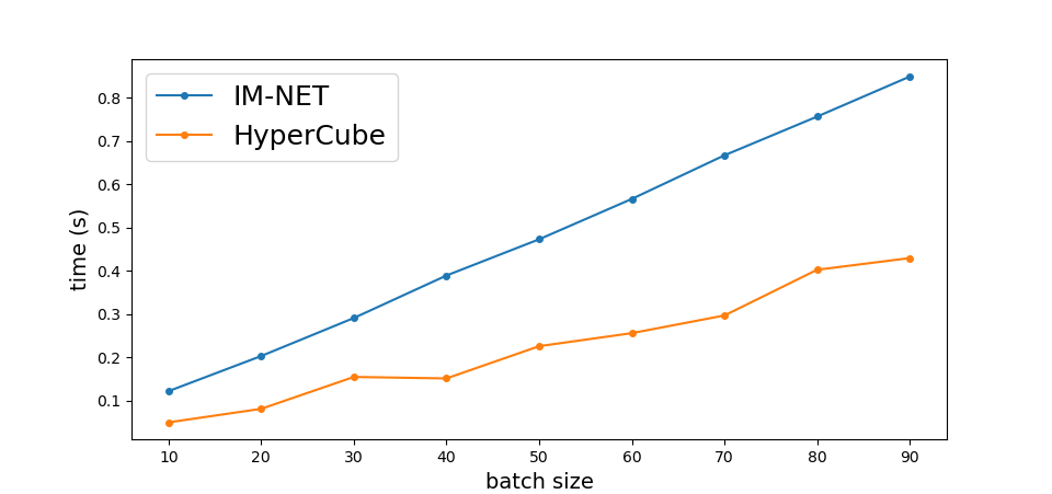
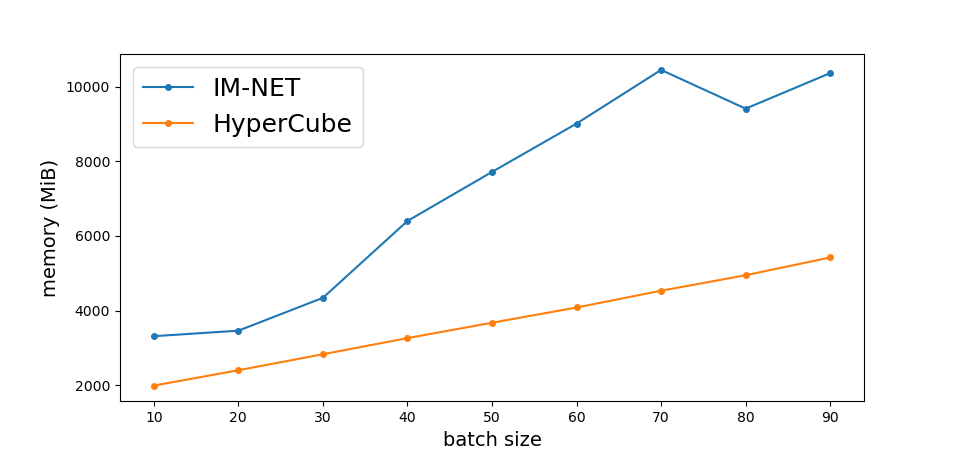
Figure 5: Comparison of training times and GPU memory used by IM-NET and HyperCube. Our HyperCube method offers over an order of magnitude decrease in both training time and memory.

Our goal is to obtain a classification rate for all elements from the interval. Therefore, we consider the worst-case prediction for the whole interval bound $[\stackunder[1.2pt]{$z$}{\rule{3.44444pt}{0.32289pt}}_{K},\bar{z}_{K}]$ of the final logits. More precisely, we need to ensure that the entire bounding box is classified correctly, i.e., no perturbation changes the correct class label. In consequence, the logit of the true class is equal to its lower bound, and the other logits are equal to their upper bounds:

$$\hat{z}_{K,y}=\left\{\begin{array}[]{ll}\overline{z}_{K,y},&\mbox{ for }y\neq y_{true},\\[3.44444pt] \underline{z}_{K,y_{true}},&\mbox{ otherwise }.\end{array}\right.$$

Finally, one can apply softmax with the cross-entropy loss to the logit vectors $\hat{z}_{K}$ representing the worst-case prediction, see Fig. 4. For more detailed information see [2, 3].

Such architecture can be simply added to HyperCube as a target network. It turns out that the output of the interval layer can be calculated only by two matrix multiplies:

$$\begin{array}[]{lll}&z_{k-1}=\frac{\bar{z}_{k-1}+\stackunder[1.2pt]{$z$}{\rule{2.41112pt}{0.22603pt}}_{k-1}}{2},&r_{k-1}=\frac{\bar{z}_{k-1}-\stackunder[1.2pt]{$z$}{\rule{2.41112pt}{0.22603pt}}_{k-1}}{2},\\[3.44444pt] &z_{k}=W_{k}z_{k-1}+b_{k-1},&r_{k}=|W_{k}|r_{k-1},\\[3.44444pt] &\stackunder[1.2pt]{$z$}{\rule{3.44444pt}{0.32289pt}}_{k}=z_{k}-r_{k},&\bar{z}_{k}=z_{k}+r_{k},\\ \end{array}$$

where $|\cdot|$ is the element-wise absolute value operator and $r_{k}$ is a radius of the interval.

Consequently, IntervalNet has exactly the same number of weights as in a fully connected architecture with the some architecture. HyperFlow is a copy of HyperCube with using IntervalNet instead of MLP as a target network. We use worst-case accuracy instead of mse to ensure that the whole voxel is correctly classified.

It should be highlighted that IntervalNet can not be added to IM-NET since we concatenate feature vectors with 3D coordinates. More precisely, feature vectors must be propagated by fully connected architecture and 3D cube by interval arithmetic, which is hard to implement in one neural network.

4 Experiments

In this section, we describe the experimental results of the proposed generative models in various tasks, including 3D mesh generation and interpolation. We show that our model is essentially faster and requires less memory in training time. Then, we compare our model with a baseline on reconstruction and generative tasks.

		Plane	Car	Chair	Rifle	Table
MSE	IM-NET	2.14	4.99	11.43	1.91	10.67
	HyperCube	2.44	4.37	9.07	1.91	9.37
IoU	IM-NET	78.77	89.26	65.65	72.88	71.44
	HyperCube	65.35	90.05	72.61	63.97	73.78
CD	IM-NET	4.23	5.44	9.05	3.77	11.54
	HyperCube	4.74	3.36	8.35	4.20	8.82

Table 1: The mean is calculated for reconstructions of 100 first elements from test set in each category. MSE is multiplied by $10^{3}$, IoU by $10^{2}$, and CD by $10^{4}$.

4.1 Training time and memory footprint comparison

Fig. 5 displays a comparison between our HyperCube method and the competing IM-NET. For a fair comparison we evaluated the architectures proposed in [1] . The models were trained on the ShapeNet dataset. Our HyperCube approach leads to a significant reduction in both training time and memory footprint due to a more compact architecture.

4.2 Reconstruction capabilities

For the quantitative comparison of our method with the current state-of-the-art solutions in the reconstruction task, we follow the approach introduced in [1]. Metrics for encoding and reconstruction are based on point-wise distances, e.g., Chamfer Distance (CD), Mean Squared Error (MSE) and Intersection over Union (IoU) on voxels.

The results are presented in Table 2. HyperCube obtain comparable results to the reference method.

		Plane	Car	Chair	Rifle	Table
MSE	IM-NET	2.98	10.98	17.11	2.41	13.38
	IM-NET %	0.45	0.70	0.68	0.56	0.64
	HyperCube	2.99	7.47	16.46	2.61	13.23
	HyperCube %	0.57	0.70	0.72	0.68	0.69
IoU	IM-NET	56.05	77.36	50.46	51.53	54.08
	IM-NET %	0.61	0.71	0.72	0.69	0.75
	HyperCube	61.68	86.34	53.52	59.80	61.23
	HyperCube %	0.67	0.71	0.76	0.73	0.77
CD	IM-NET	7.38	5.72	13.99	8.06	17.36
	IM-NET	0.58	0.71	0.78	0.72	0.82
	HyperCube	5.02	4.28	12.92	4.96	12.49
	HyperCube %	0.66	0.74	0.78	0.74	0.81

Table 2: Generation. Mean of minimum MSE/CD, maximum IoU between test set and 5*test_set_size generated objects, % of test set objects matched as the closest ones.

4.3 Generative model

We examine the generative capabilities of the provided HyperCube model compared to the existing reference IM-NET. Our model similarly to IM-NET can be used for generating 3D objects. For 3D shape generation, we employed latent-GANs [42] on feature vectors learned by a 3D autoencoder. By analogy to IM-NET we did not apply traditional GANs trained on voxel grids since the training set is considerably smaller compared to the size of the output. Therefore, the pre-trained AE serves as a dimensionality reduction method, and the latent-GAN was trained on high-level features of the original shapes. In Table 2 we present compression between IM-NET and HyperCube. As we can see we obtain similar results than classical approaches.

input
HyperCube
HyperCube (Interval)

Figure 6: Competition between models between architectures working on points (HyperCube) and interval architecture (HyperFlow). As we can see, IntervalNet can fill some empty spaces in meshes.

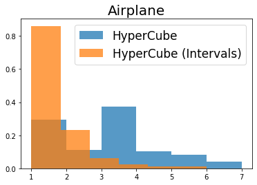
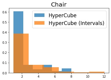
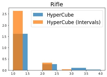
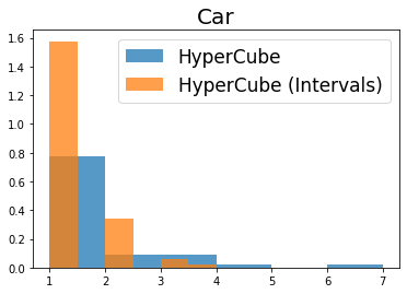
Figure 7: We calculate the number of connected components produced by mesh obtained by architecture with intervals and without. Our HyperFlow approach provides better models for classes Airplane, Rifle, Car.

4.4 Intervals vs Points

As it was shown in previous section, HyperFlow is essentially faster than IM-NET. Both architectures give similar reconstruction and generative capability. Since HyperCube as well as IM-NET works directly on points the classification boundary is not smooth and we can see artifacts in mesh reconstruction, see Fig. 6. Since mesh representation is produced by the Marching Cubes algorithm such artefacts appear with object with similar value of MSE, CD, and IoU. As it was shown in [1, 43] such measures do not describe visual quality.

The classification boundary can be regularized using IntervalNet. In Fig. 6 we present such examples. As we can see HyperFlow models produce single objects without empty space. To verify it, we calculate the number of connected components produced by mesh and visualize them on histograms, see Fig. 7. Our model produces better models for classes: Airplane, Rifle, Car. On the other hand, in the Tables, we have a similar result.

5 Conclusions

In this work we introduce a new implicit field representation of 3D models. Contrary to the existing solutions, such as IM-NET, it is more light-weight and faster to train thanks to the hypernetwork architecture, while offering competitive or superior quantitative results. Finally, our method allows to incorporate interval arithmetic which enables processing entire 3D voxels, instead of their sampled version, and hence yielding more plausible and higher quality 3D reconstructions.

References

- [1] Zhiqin Chen and Hao Zhang. Learning implicit fields for generative shape modeling. In Proceedings of the IEEE/CVF Conference on Computer Vision and Pattern Recognition, pages 5939–5948, 2019.
- [2] Sven Gowal, Krishnamurthy Dvijotham, Robert Stanforth, Rudy Bunel, Chongli Qin, Jonathan Uesato, Relja Arandjelovic, Timothy Mann, and Pushmeet Kohli. On the effectiveness of interval bound propagation for training verifiably robust models. arXiv preprint arXiv:1810.12715, 2018.
- [3] Pawel Morawiecki, Przemysław Spurek, Marek Śmieja, and Jacek Tabor. Fast and stable interval bounds propagation for training verifiably robust models. arXiv preprint arXiv:1906.00628, 2019.
- [4] Christopher B Choy, Danfei Xu, JunYoung Gwak, Kevin Chen, and Silvio Savarese. 3d-r2n2: A unified approach for single and multi-view 3d object reconstruction. In European conference on computer vision, pages 628–644. Springer, 2016.
- [5] Rohit Girdhar, David F Fouhey, Mikel Rodriguez, and Abhinav Gupta. Learning a predictable and generative vector representation for objects. In European Conference on Computer Vision, pages 484–499. Springer, 2016.
- [6] Yiyi Liao, Simon Donne, and Andreas Geiger. Deep marching cubes: Learning explicit surface representations. In Proceedings of the IEEE Conference on Computer Vision and Pattern Recognition, pages 2916–2925, 2018.
- [7] Jiajun Wu, Chengkai Zhang, Tianfan Xue, William T Freeman, and Joshua B Tenenbaum. Learning a probabilistic latent space of object shapes via 3d generative-adversarial modeling. In Proceedings of the 30th International Conference on Neural Information Processing Systems, pages 82–90, 2016.
- [8] Christian Häne, Shubham Tulsiani, and Jitendra Malik. Hierarchical surface prediction for 3d object reconstruction. In 2017 International Conference on 3D Vision (3DV), pages 412–420. IEEE, 2017.
- [9] Gernot Riegler, Ali Osman Ulusoy, Horst Bischof, and Andreas Geiger. Octnetfusion: Learning depth fusion from data. In 2017 International Conference on 3D Vision (3DV), pages 57–66. IEEE, 2017.
- [10] Maxim Tatarchenko, Alexey Dosovitskiy, and Thomas Brox. Octree generating networks: Efficient convolutional architectures for high-resolution 3d outputs. In Proceedings of the IEEE International Conference on Computer Vision, pages 2088–2096, 2017.
- [11] Peng-Shuai Wang, Chun-Yu Sun, Yang Liu, and Xin Tong. Adaptive o-cnn: A patch-based deep representation of 3d shapes. ACM Transactions on Graphics (TOG), 37(6):1–11, 2018.
- [12] Amir Arsalan Soltani, Haibin Huang, Jiajun Wu, Tejas D Kulkarni, and Joshua B Tenenbaum. Synthesizing 3d shapes via modeling multi-view depth maps and silhouettes with deep generative networks. In Proceedings of the IEEE conference on computer vision and pattern recognition, pages 1511–1519, 2017.
- [13] Chen-Hsuan Lin, Chen Kong, and Simon Lucey. Learning efficient point cloud generation for dense 3d object reconstruction. In proceedings of the AAAI Conference on Artificial Intelligence, volume 32, 2018.
- [14] Hang Su, Subhransu Maji, Evangelos Kalogerakis, and Erik Learned-Miller. Multi-view convolutional neural networks for 3d shape recognition. In Proceedings of the IEEE international conference on computer vision, pages 945–953, 2015.
- [15] Panos Achlioptas, Olga Diamanti, Ioannis Mitliagkas, and Leonidas Guibas. Learning representations and generative models for 3d point clouds. In International conference on machine learning, pages 40–49. PMLR, 2018.
- [16] Haoqiang Fan, Hao Su, and Leonidas J Guibas. A point set generation network for 3d object reconstruction from a single image. In Proceedings of the IEEE conference on computer vision and pattern recognition, pages 605–613, 2017.
- [17] Charles R Qi, Hao Su, Kaichun Mo, and Leonidas J Guibas. Pointnet: Deep learning on point sets for 3d classification and segmentation. In Proceedings of the IEEE conference on computer vision and pattern recognition, pages 652–660, 2017.
- [18] Charles R Qi, Li Yi, Hao Su, and Leonidas J Guibas. Pointnet++: Deep hierarchical feature learning on point sets in a metric space. arXiv preprint arXiv:1706.02413, 2017.
- [19] Yaoqing Yang, Chen Feng, Yiru Shen, and Dong Tian. Foldingnet: Point cloud auto-encoder via deep grid deformation. In Proceedings of the IEEE Conference on Computer Vision and Pattern Recognition, pages 206–215, 2018.
- [20] Ayan Sinha, Jing Bai, and Karthik Ramani. Deep learning 3d shape surfaces using geometry images. In European Conference on Computer Vision, pages 223–240. Springer, 2016.
- [21] Ayan Sinha, Asim Unmesh, Qixing Huang, and Karthik Ramani. Surfnet: Generating 3d shape surfaces using deep residual networks. In Proceedings of the IEEE conference on computer vision and pattern recognition, pages 6040–6049, 2017.
- [22] Nanyang Wang, Yinda Zhang, Zhuwen Li, Yanwei Fu, Wei Liu, and Yu-Gang Jiang. Pixel2mesh: Generating 3d mesh models from single rgb images. In Proceedings of the European Conference on Computer Vision (ECCV), pages 52–67, 2018.
- [23] Jun Li, Kai Xu, Siddhartha Chaudhuri, Ersin Yumer, Hao Zhang, and Leonidas Guibas. Grass: Generative recursive autoencoders for shape structures. ACM Transactions on Graphics (TOG), 36(4):1–14, 2017.
- [24] Chenyang Zhu, Kai Xu, Siddhartha Chaudhuri, Renjiao Yi, and Hao Zhang. Scores: Shape composition with recursive substructure priors. ACM Transactions on Graphics (TOG), 37(6):1–14, 2018.
- [25] Emilien Dupont, Yee Whye Teh, and Arnaud Doucet. Generative models as distributions of functions. arXiv preprint arXiv:2102.04776, 2021.
- [26] Lars Mescheder, Michael Oechsle, Michael Niemeyer, Sebastian Nowozin, and Andreas Geiger. Occupancy networks: Learning 3d reconstruction in function space. In Proceedings of the IEEE/CVF Conference on Computer Vision and Pattern Recognition, pages 4460–4470, 2019.
- [27] Songyou Peng, Michael Niemeyer, Lars Mescheder, Marc Pollefeys, and Andreas Geiger. Convolutional occupancy networks. In Computer Vision–ECCV 2020: 16th European Conference, Glasgow, UK, August 23–28, 2020, Proceedings, Part III 16, pages 523–540. Springer, 2020.
- [28] Mateusz Michalkiewicz, Jhony K Pontes, Dominic Jack, Mahsa Baktashmotlagh, and Anders Eriksson. Implicit surface representations as layers in neural networks. In Proceedings of the IEEE/CVF International Conference on Computer Vision, pages 4743–4752, 2019.
- [29] Jeong Joon Park, Peter Florence, Julian Straub, Richard Newcombe, and Steven Lovegrove. Deepsdf: Learning continuous signed distance functions for shape representation. In Proceedings of the IEEE/CVF Conference on Computer Vision and Pattern Recognition, pages 165–174, 2019.
- [30] Guandao Yang, Xun Huang, Zekun Hao, Ming-Yu Liu, Serge Belongie, and Bharath Hariharan. Pointflow: 3d point cloud generation with continuous normalizing flows. In Proceedings of the IEEE International Conference on Computer Vision, pages 4541–4550, 2019.
- [31] Przemysław Spurek, Sebastian Winczowski, Jacek Tabor, Maciej Zamorski, Maciej Zięba, and Tomasz Trzciński. Hypernetwork approach to generating point clouds. Proceedings of the 37th International Conference on Machine Learning (ICML), 2020.
- [32] Przemysław Spurek, Maciej Zięba, Jacek Tabor, and Tomasz Trzciński. Hyperflow: Representing 3d objects as surfaces. arXiv preprint arXiv:2006.08710, 2020.
- [33] Ruojin Cai, Guandao Yang, Hadar Averbuch-Elor, Zekun Hao, Serge Belongie, Noah Snavely, and Bharath Hariharan. Learning gradient fields for shape generation. In Computer Vision–ECCV 2020: 16th European Conference, Glasgow, UK, August 23–28, 2020, Proceedings, Part III 16, pages 364–381. Springer, 2020.
- [34] David Ha, Andrew Dai, and Quoc V Le. Hypernetworks. arXiv preprint arXiv:1609.09106, 2016.
- [35] Przemysław Spurek, Artur Kasymov, Marcin Mazur, Diana Janik, Slawomir Tadeja, Lukasz Struski, Jacek Tabor, and Tomasz Trzciński. Hyperpocket: Generative point cloud completion. arXiv preprint arXiv:2102.05973, 2021.
- [36] Przemysław Spurek, Sebastian Winczowski, Maciej Zięba, Tomasz Trzciński, and Kacper Kania. Modeling 3d surface manifolds with a locally conditioned atlas. arXiv preprint arXiv:2102.05984, 2021.
- [37] Germund Dahlquist and Åke Björck. Numerical methods in scientific computing, volume I. SIAM, 2008.
- [38] S Chakraverty and Deepti Moyi Sahoo. Interval response data based system identification of multi storey shear buildings using interval neural network modelling. Computer Assisted Methods in Engineering and Science, 21(2):123–140, 2014.
- [39] S Chakraverty and Deepti Moyi Sahoo. Novel transformation-based response prediction of shear building using interval neural network. Journal of Earth System Science, 126(3):32, 2017.
- [40] Deepti Moyi Sahoo and S Chakraverty. Structural parameter identification using interval functional link neural network. In Recent Trends in Wave Mechanics and Vibrations, pages 139–150. Springer, 2020.
- [41] Kwang Hyung Lee. First course on fuzzy theory and applications, volume 27. Springer Science & Business Media, 2004.
- [42] Chao Dong, Chen Change Loy, Kaiming He, and Xiaoou Tang. Learning a deep convolutional network for image super-resolution. In European conference on computer vision, pages 184–199. Springer, 2014.
- [43] Olga Sorkine, Daniel Cohen-Or, and Sivan Toledo. High-pass quantization for mesh encoding. In Symposium on Geometry Processing, volume 42, page 3. Citeseer, 2003.