Estimation of Photometric Redshifts. I. Machine Learning Inference for Pan-STARRS1 Galaxies Using Neural Networks

Abstract

We present a new machine learning model for estimating photometric redshifts with improved accuracy for galaxies in Pan-STARRS1 data release 1. Depending on the estimation range of redshifts, this model based on neural networks can handle the difficulty for inferring photometric redshifts. Moreover, to reduce bias induced by the new model’s ability to deal with estimation difficulty, it exploits the power of ensemble learning. We extensively examine the mapping between input features and target redshift spaces to which the model is validly applicable to discover the strength and weaknesses of trained model. Because our trained model is well calibrated, our model produces reliable confidence information about objects with non-catastrophic estimation. While our model is highly accurate for most test examples residing in the input space, where training samples are densely populated, its accuracy quickly diminishes for sparse samples and unobserved objects (i.e., unseen samples) in training. We report that out-of-distribution (OOD) samples for our model contain both physically OOD objects (i.e., stars and quasars) and galaxies with observed properties not represented by training data. The code for our model is available at https://github.com/GooLee0123/MBRNN for other uses of the model and retraining the model with different data.

1 Introduction

For various astronomical studies, the photometric redshifts of galaxies are critical. Representative research areas include cosmological model testing (Blake & Bridle, 2005; Amon et al., 2018) and dark energy survey (Banerji et al., 2008; Sánchez et al., 2014). In terms of accuracy, although the spectroscopic estimation of redshifts is the most appropriate method, acquiring spectroscopic redshifts is significantly more expensive than estimating photometric redshifts (Salvato et al., 2019). In terms of cost, at a tolerable expense of accuracy, photometric redshifts can be a suitable substitute for spectroscopic redshifts.

Modern photometric redshift estimation approaches are split into two large branches: the spectral energy distribution (SED) fitting based on SED models (including spectral templates) and machine learning inference (Cavuoti et al., 2017; Salvato et al., 2019). These two methods are mutually complementary with different pros and cons. The template-based SED fitting may provide photometric redshifts in a wide redshift and photometric range; moreover, using Bayesian inference improves the effectiveness of the method (Bolzonella et al., 2000). However, this approach heavily relies on the prior knowledge of SEDs and the understanding of related physics determining SEDs. This dependency may result in biased results (Walcher et al., 2011; Tanaka, 2015). However, the machine learning method can quickly retrieve accurate photometric redshifts without dependence on prior knowledge (Cavuoti et al., 2017). Nonetheless, most of the machine learning models suffer from performance degradation for few or unseen data during their training since these methods are induction models for the provided data (Liang et al., 2018; Hendrycks et al., 2019).

Samples drawn from out-of-distribution (OOD) (i.e., few or unseen data in training) are well-known distress in a reliable application of neural networks (NNs). Hendrycks & Gimpel (2017) demonstrate that an ML model’s accuracy degrades for OOD samples for several training datasets: e.g., MNIST (LeCun & Cortes, 2010), CIFAR-10, and CIFAR-100 (Krizhevsky, 2012), and they suggest a baseline model for OOD detection in an NN. Lee et al. (2018) propose an advanced method for detecting OOD examples using Mahalanobis distance, thus assuming the trained network parameters can be fitted by a class-conditional Gaussian distribution. The unsupervised approach introduced by Yu & Aizawa (2019) uses unlabeled samples as training data to equip NNs with the functionality of scoring and detecting OOD examples. A parameter-free OOD score is proposed by Serrà et al. (2020) to handle the OOD issue in generative models, thus posing that the problem is attributed to the excessive effect of input complexity. These recent studies emphasize that, for achieving a more robust NN model, the OOD instance is a practical and important limitation.

The appropriate warning on OOD samples and handling their impact on models should be offered in machine learning inference of photometric redshifts. The machine learning method for photometric redshift estimation has been explored in many past studies (Firth et al., 2003; Ball et al., 2008; Singal et al., 2011; Brescia et al., 2013; Laigle et al., 2017; Bilicki et al., 2018; Chong & Yang, 2019). In these past studies, although the superior performance of machine learning methods has been demonstrated, the input/target feature spaces regarding OOD examples that the models are unable to describe for accurate and reliable prediction of photometric redshifts have not been quantitatively investigated.

In this series of studies, we propose a machine learning method to improve the accuracy and reliability of photometric redshift inference, thus exploiting the well-known flexibility of NN models. The NNs are renowned for their capacity of mapping nonlinear relationships between input and target (i.e., redshift) as a universal approximator and handling a massive amount of data. NNs have been one of the most popularly used machine learning algorithms throughout a wide range of fields and tasks including natural language processing (Vaswani et al., 2017; Brown et al., 2020), image classification (Krizhevsky et al., 2012; Szegedy et al., 2015), autonomous vehicles (Levinson et al., 2011; Dosovitskiy et al., 2017), and protein structure prediction (Senior et al., 2020; Torrisi et al., 2020).

This study, the first study in the series, focuses on improving accuracy in inferring photometric redshifts. In our NN models, we adopt anchor loss (Ryou et al., 2019), which considers the difficulty of inferring photometric redshifts with respect to the estimated redshift, i.e., target. The primary cause of the inference difficulty is imbalanced training samples for redshifts and complex patterns in mapping from input features to the target redshift space. Because a new loss can cause systematic bias effects, we use an ensemble learning approach, which combines multiple base models into a unified model, to reduce the bias of models and improve accuracy (Zhou, 2009).

Photometric data used are collected from the Panoramic Survey Telescope and Rapid Response System (Pan-STARRS) public data release (Chambers et al., 2016). We intend to use our trained model to infer the photometric redshifts of objects that correspond to extragalactic transient and variable sources. For transient sources such as supernovae and variable sources such as quasars, Pan-STARRS photometric catalogs can be useful to infer the photometric redshifts of hosts. Because photometric information used by our model is not much different from that acquired in other surveys, such as the SkyMapper Southern Sky Survey (Keller et al., 2007) and Legacy Survey of Space and Time (Tyson, 2002; Ivezić et al., 2019), using the Pan-STARRS data for the model has potential benefits for applications with other data. Moreover, there are not many previous studies on photometric redshifts with Pan-STARRS data (Beck et al., 2021).

This study is organized as follows. Section 2 provides the overview of training data and pre-processing of input features for machine learning applications. In Section 3, machine learning approaches and performance evaluation metrics are elaborated in detail. Section 4 focuses on the performance analysis of our machine learning model and its comparison with baseline models. In Section 5, we explore the mapping between the input feature space and the target redshift space for which our model is validly applicable using comparison data. Finally, we discuss our results and provide the conclusion in Section 6.

2 Data

Table 1: Spectroscopic galaxy redshift samples.

Dataset name	Number of objects	Selection conditions	Reference
SDSS DR15	1294042	(CLASS $==$ GALAXY) and (ZWARNING $==$ 0 or 16) and (Z_ERR $>=$ 0.0)	Aguado et al. (2019)
LAMOST DR5	116186	(CLASS $==$ GALAXY) and (Z $>$ -9000)	Cui et al. (2012)
6dFGS	45036	(QUALITY_CODE $==$ 4) and (REDSHIFT $<=$ 1.0)	Jones et al. (2009)
PRIMUS	11012	(CLASS $==$ GALAXY) and (ZQUALITY $==$ 4)	Cool et al. (2013)
2dFGRS	7000	(Q_Z $>=$ 4) and (O_Z_EM $<$ 1) and (Z $<$ 1)	Colless et al. (2001)
OzDES	2159	(TYPES $!=$ RadioGalaxy or AGN or QSO or Tertiary) and (FLAG $!=$ 3 and 6) and (Z $>$ 0.0001)	Childress et al. (2017)
VIPERS	1680	(4 $<=$ ZFLG $<$ 5) or (24 $<=$ ZFLG $<$ 25)	Scodeggio et al. (2018)
COSMOS-Z-COSMOS	985	((4 $<=$ CC $<$ 5) or (24 $<=$ CC $<$ 25)) and (REDSHIFT $>=$ 0.0002)	Lilly et al. (2007, 2009)
VVDS	829	ZFLAGS $==$ 4 or 24	Le Fèvre et al. (2013)
DEEP2	540	(ZBEST $>$ 0.001) and (ZERR $>$ 0.0) and (ZQUALITY $==$ 4) and (CLASS $==$ GALAXY)	Newman et al. (2013)
COSMOS-DEIMOS	517	(REMARKS $!=$ STAR) and (QF $<$ 10) and (Q $>=$ 1.6)	Hasinger et al. (2018)
COMOS-Magellan	183	(CLASS $==$ nl or a or nla) and (Z_CONF $==$ 4)	Trump et al. (2009)
C3R2-Keck	88	(REDSHIFT $>=$ 0.001) and (REDSHIFT_QUALITY $==$ 4)	Masters et al. (2017, 2019)
MUSE-Wide	3	No filtering conditions.	Urrutia et al. (2019)
UVUDF	2	Spectroscopic samples.	Rafelski et al. (2015)

Training samples comprise 1,480,262 galaxy objects with known spectroscopic redshifts. We compile the samples from multiple spectroscopic redshift catalogs with the condition of reliable redshift estimation. Table 1 summarizes the spectroscopic redshift samples that satisfy the required selection conditions and have acceptable photometric data as subsequently described. Most selection conditions adopted here help us use only samples with highly reliable redshifts.

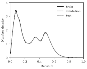
Figure 1: Redshift distributions of training, validation, and test sets. We use an adaptive kernel density estimation for density estimation of redshifts.

We use the photometric data of Pan-STARRS project as input photometric data for the machine learning model. The Pan-STARRS1 (PS1) is the first 1.8m telescope of the Pan-STARRS project (Kaiser et al., 2010), and the $3\pi$ Steradian Survey is one of the primary surveys covering 75% of the sky (Chambers et al., 2016). The PS1 survey provides photometry in five grizy bands with limiting magnitudes of 23.3, 23.2, 23.1, 22.3, and 21.4, respectively (Chambers et al., 2016).

We retrieve the photometric data of spectroscopic samples from the public data release 1 (DR1, Flewelling et al., 2020) using the Vizier table, which has objects included in the ObjectThin and StackObjectThin tables with nDetections $>$ 2 option. For given positions of spectroscopic samples, we search the nearest object in the photometric table using the search radius of 0.5 arcseconds with the condition of ObjectQualityFlags $==$ QF_OBJ_GOOD (i.e., good-quality measurement in the PS1) (Flewelling et al., 2020). A single photometric object can be matched to multiple spectroscopic samples. We use the median redshift if more than two spectroscopic samples correspond to a single PS1 DR1 object. We use the average of two redshifts if two spectroscopic samples are matched to a single photometric object and their redshift difference is less than or equal to 0.005. Objects with a difference of greater than 0.005 are excluded from training samples.

We purposely restrict our training input data to color-related features that allow the easy interpretation of the model results rather than exploring all possible combinations of input features (D’Isanto et al., 2018). The input features comprise four colors $(g-r)$, $(r-i)$, $(i-z)$, and $(z-y)$ in PSF measurement, their uncertainties derived in the quadrature rule, and the same quantities in Kron measurement. The training data include objects only if all four colors are valid in the data release.

Magnitudes of samples are excluded as input; rather, we include the color and color difference uncertainties that implicitly depend on the magnitude and SED of sources. As expected, fainter objects have larger uncertainties. Although uncertainties implicitly contain information correlated with the source magnitudes and SEDs, how NN models treat these inputs may be different.

Furthermore, the $E(B-V)$ value is one of the input features. It is common to apply Galactic dust extinction correction to photometric data as a pre-processing step before photometric redshifts are estimated by machine learning methods. In our case, we let the machine learning models consider the effect of the Galactic dust extinction in the training stage (Beck et al., 2021). We decide to use the $E(B-V)$ values based on the dust emission model of the Plank cosmic microwave background observation (Planck Collaboration et al., 2014), which provides a wide coverage of the sky.

The input features are transformed to improve the performance of the machine learning model. In training machine learning models, data pre-processing is required when input features have different ranges (Sola & Sevilla, 1997). Diversely ranged features have a different effect on the loss function adopted in a machine learning model, thus making results biased. From the geometrical standpoint, the data points of differently ranged features form a multi-dimensional asymmetric volume in the input space. Data pre-processing handles this geometrical asymmetry and makes data more symmetric. Moreover, it smooths out pointy regions that might exist on the surface of the volume. Our data pre-processing restricts each feature to a comparable range. We test two data pre-processing methods: min-max normalization and standardization. Both methods process data in a feature-wise manner. The former method uses the minimum and maximum values of each feature to restrict feature ranges. For standardization, each feature is re-scaled to have zero mean and unit variance.

After the pre-processing step, we randomly select 80% of our samples as the training set and each 10% of samples as the test and validation sets, respectively. Because we randomly split the data and have many samples, we assume that the samples allocated to each set are drawn from the same distribution. Figure 1 shows the redshift distribution of the training, test, and validation sets. To avoid any confusion, we sometimes refer to redshifts as targets in training the machine learning models.

3 Method

In this section, we describe the baseline models based on regression, our machine learning approach, ensemble methods for better machine learning performance, and metrics to quantitatively assess the photometric redshift quality.

3.1 Baseline Models Based on Regression

For both classification and regression, K-nearest neighbors (KNN) is a relatively simple non-parametric model that can be used (Altman, 1992). Because of its simplicity, the model has been used to estimate the photometric redshifts of galaxies and quasars or used as a baseline to evaluate the performances of novel approaches (Zhang et al., 2013; Pasquet-Itam & Pasquet, 2018). The model estimates targets (or labels) of given samples based on the averaged target values of $k$ nearest samples in a training set.

Random forest (RF) is an ensemble method using multiple decision trees (Breiman, 2001). The model has been extensively used for astronomical classification, regression, and other tasks (Zhang & Zhao, 2015). RF is essentially optimized to use feature-based inputs because it recursively splits high-dimensional features by generating multiple root nodes and their succeeding child nodes. RF, in addition to KNN, is frequently used as a baseline because of its usage of ensemble learning resulting in statistical robustness and its split-rule-learning characteristics, which can return the importance of input features.

A NN is a representative machine learning model inspired by the functioning of the human brain (Hopfield, 1982). Generally, NN architecture comprises one input layer, multiple hidden layers, and one output layer. Moreover, these layers are composed of artificial neurons or perceptrons (Rosenblatt, 1958), which are the basic units forming the model and mimicking biological neurons. Artificial neurons are interconnected to ones in adjacent layers with randomly initialized connection weights. Vectors provided to neurons in the input layer are transformed by neurons in the hidden layers using connection weights with nonlinear activation functions and are then transmitted to the output layer. Then, neurons in the output layer finally produce scalar or vector outputs. Although the definition of the term is not stringent, the network is usually referred to as a vanilla NN (VNN) when the model generates a scalar output. We emphasize that the regression NN, hereafter, is referred to as VNN because, in our study, it produces a scalar output — a photometric redshift.

We use the mean squared error (MSE) as a loss function to train the parameters of RF and VNN for redshift regression. KNN does not require a loss function. Moreover, we also have tested the adaptive robust loss function proposed by Barron (2019), thus reflecting the anchor loss to be explained later. However, we found that a simpler MSE outperforms the loss in this study.

3.2 Multiple-Bin Regression with NN

The MSE for regression problems with the heterogeneous target is not an optimal option (Liu, 2019). MSE is the most commonly used loss function to train machine learning models for regression because minimizing the MSE is generally identical for maximizing log-likelihood from a probabilistic standpoint. In most real-life cases, however, the target is heterogeneous rather than homogeneous. If it is the case, using the MSE may result in an undesirable performance of the regression model because the loss function fosters the model to minimize the error throughout all modes while not considering the multi-modal behavior of the target.

Because our target, i.e., redshift, can have a multi-modal distribution particularly because of the degeneracy of redshifts in terms of input features, we consider multiple-bin regression with a NN (hereafter, MBRNN) to bypass the limitation of the MSE for a heterogeneously behaving target. The MBRNN model has been previously explored in several studies for viewpoint estimation (Su et al., 2015; Francisco Massa & Aubry, 2016), bounding-box estimation (Mousavian et al., 2017), pose estimation (Kundu et al., 2018), and redshift estimation in astronomy (Pasquet-Itam & Pasquet, 2018; Pasquet et al., 2019). Compared with regression using the MSE, these studies demonstrated the performance enhancement of the approach. Furthermore, the property of the probabilistic model enables deeper scrutiny on the causes of poor inference performance for specific samples and examination of model calibration, which are discussed in Section 4.1.

We first discretize spectroscopic redshifts and divide them into $n$ independent bins. We test two types of redshift bins: uniform and non-uniform. For uniform bins, we equally discretize the redshifts of the training data with a constant bin width. However, we make each bin have an almost uniform number of samples in the non-uniform binning. Because most objects reside in low redshift ranges, the non-uniform bin width becomes wider as the redshift increases even though it is not monotonic.

The MBRNN model using the softmax function estimates probabilities $p_{i}$ that the photometric redshifts of objects lie in $i^{th}$ redshift bin. That is, we modify the regression problem into a classification problem with multiple redshift bins. For point estimation, we can compute the photometric redshift $z_{phot}$ either by selecting a redshift bin center with peak probability (i.e., mode) as $z_{mode}$ or by averaging with the output probabilities and central values of the bins as $z_{avg}$ as follows:

$$\begin{split}z_{mode}&=c_{j}~{}{\rm for}~{}j=\underset{k}{\operatorname{argmax}}(p_{k}),\\ {\rm or}\\ z_{avg}&=\sum p_{i}\,c_{i},\\ \end{split}$$ (1)

where $c_{i}$ is the central value of ${i^{th}}$ redshift bin. We compare the prediction accuracy of the two different point-estimation methods in Section 4.

We use the anchor loss (Ryou et al., 2019) as a classification loss function for training the model. The loss is designed to measure the disparity of two given probability distributions considering prediction difficulties, which can be attributed to various reasons such as the scarcity of data or the similarities between samples drawn from different distributions. This function evaluates the prediction difficulty using the difference between network-estimated probabilities for the true and other classes. In an easy prediction case, the network-estimated probability of the true class is higher than those of the other classes, whereas it is lower in a difficult case. The difficulty is used to weigh the loss of a sample. For the given two discrete probability distributions, $g$ and $p$, the anchor loss $\ell(g,p)$ is defined as follows:

$$\ell(g,p)=-\underset{k}{\sum}\,g_{k}\,log(p_{k})+(1-g_{k})(1+p_{k}-p_{*})^{\gamma}log(1-p_{k}),$$ (2)

where $g_{k}$ and $p_{k}$ represent the label (i.e., $g_{k}=1$ for the correct redshift bin and $g_{k}=0$ for other bins) and network-estimated probabilities for class (i.e., redshift bin) $k$, respectively; $\gamma$ represents an exponent governing the weights of prediction difficulties; $p_{*}$ represents the anchor probability which is set to the network-estimated true class probability (i.e., the classification probability for the correct redshift bin). Therefore, $p_{*}$ determines the prediction difficulties of samples. In the cases of easy prediction, the trained model assigns high probability on the true class (i.e., the correct redshift bin), leading to higher $p_{*}$ than $p_{k}$ (see the appendix of Ryou et al. (2019) and its equation A-3). Note that the anchor loss approaches a binary cross-entropy loss, which is one of the most commonly used classification losses, as $\gamma$ goes to $0$.

The baseline VNN and our proposed model MBRNN share the same NN structures except for output layers because these networks generate differently shaped outputs. The networks are composed of fully connected layers only: an input layer with 17 neurons, eight hidden layers sequentially with 128, 256, 512, 1024, 512, 256, 128, and 32 neurons, and the output layer with the number of neurons corresponding to the output size. Each layer is followed by a batch normalization layer (Ioffe & Szegedy, 2015) and softplus activation function (Zheng et al., 2015).

3.3 Ensemble of multiple-bin method

Our adoption of ensemble methods combines the outputs of multiple MBRNN models and generates an integrated model. Ensemble methods have been extensively used in the field of machine learning to overcome the limitations of models trained for a limited set of tasks. This strategy often results in better or more generalized model performance by weighting the models depending on their performance or properly assigning each model to the task where the model performs best.

To identify a suitable ensemble approach for our purpose, we evaluate four different methods: plain model averaging ensemble (E1), weighted model ensemble (E2), bin ensemble (E3), and bin-wise selective ensemble (E4) (Yu-yan, 2010). E1 is simply averaging results from each model. For E1, the performance of the integrated model might be downgraded when a poorly performing model is included because this method does not consider the specialty of each model. E2 uses weighted averaging of predictions from each model. Assigning higher and lower weights to high- and low-performance models, respectively, this method is frequently expected to yield higher performance than a single model or E1. Optimal weights can be found by various methods such as Bayesian optimization methods (Snoek et al., 2012) and gradient descent methods (Bottou, 2010). The gradient descent method with the validation set is used in our study. Moreover, we consider another weighted ensemble method E3, which allocates individual weight to each model and redshift bin combination. Because it provides different weights to each bin in addition to models, this approach has additional parameters to be tuned and more flexibility than E2. Finally, we evaluate the selective ensemble method E4, which selects a single model for each redshift bin where the model shows the highest point estimation accuracy using the validation set. In E4, we find redshift bins to which point-estimated redshifts of each test object belong using the vote of the single models. Then, the model allocated to the bin is used to estimate probability distributions for objects.

3.4 Metric

We use multiple metrics to assess performance in estimating photometric redshifts. We refer to Cavuoti et al. (2017) for the detailed description of metrics. The following is a brief explanation of metrics:

• Bias: the absolute mean of redshift differences defined by $\frac{1}{N}|\sum_{i}^{N}\Delta z_{i}|$ where $N$ represents the number of samples in the dataset, $i$ represents the sample index, and $\Delta z_{i}=(z_{i,spec}-z_{i,phot})/(1+z_{i,spec})$,

• MAD: the mean of absolute differences defined by $\frac{1}{N}\sum_{i}^{N}|\Delta z_{i}|$,

• $\sigma$: the standard deviation of the difference $z_{i,spec}-z_{i,phot}$,

• $\sigma_{68}$: the 68th percentile of the absolute difference, i.e., $|z_{i,spec}-z_{i,phot}|$,

• NMAD: the normalized median absolute deviation of the differences, which is $1.4826\times Median(\Delta z)$,

• $R_{cat}$: catastrophic (hereafter, cat) error, which corresponds to $|\Delta z|>0.15$, fraction.

Using these metrics, we evaluate the quality of photometric redshifts and perform a grid search to identify the empirically optimal configuration of the MBRNN model. For the numerical metrics, the lower the values, the better the model performance.

4 Result

4.1 Single Model Performance Test

Figure 2: Redshift difference distributions of the MBRNN and baseline models. The distribution of spectroscopic redshifts is also drawn here for comparison. The spectroscopic redshift distribution is scaled down by half for visual clarity. Positive and negative differences indicate under- and over-estimation of the distribution, respectively.

Figure 3: Distributions of spectroscopic and photometric redshifts obtained by the MBRNN and baseline models. The markers are color-coded with number density, and the color is normalized in the log scale for better contrast. Samples outside the dashed lines on both sides correspond to cat objects, and the central dashed line has a slope of 1. The Pearson correlation coefficients $\rho$ between spectroscopic and photometric redshifts are also presented in each panel.

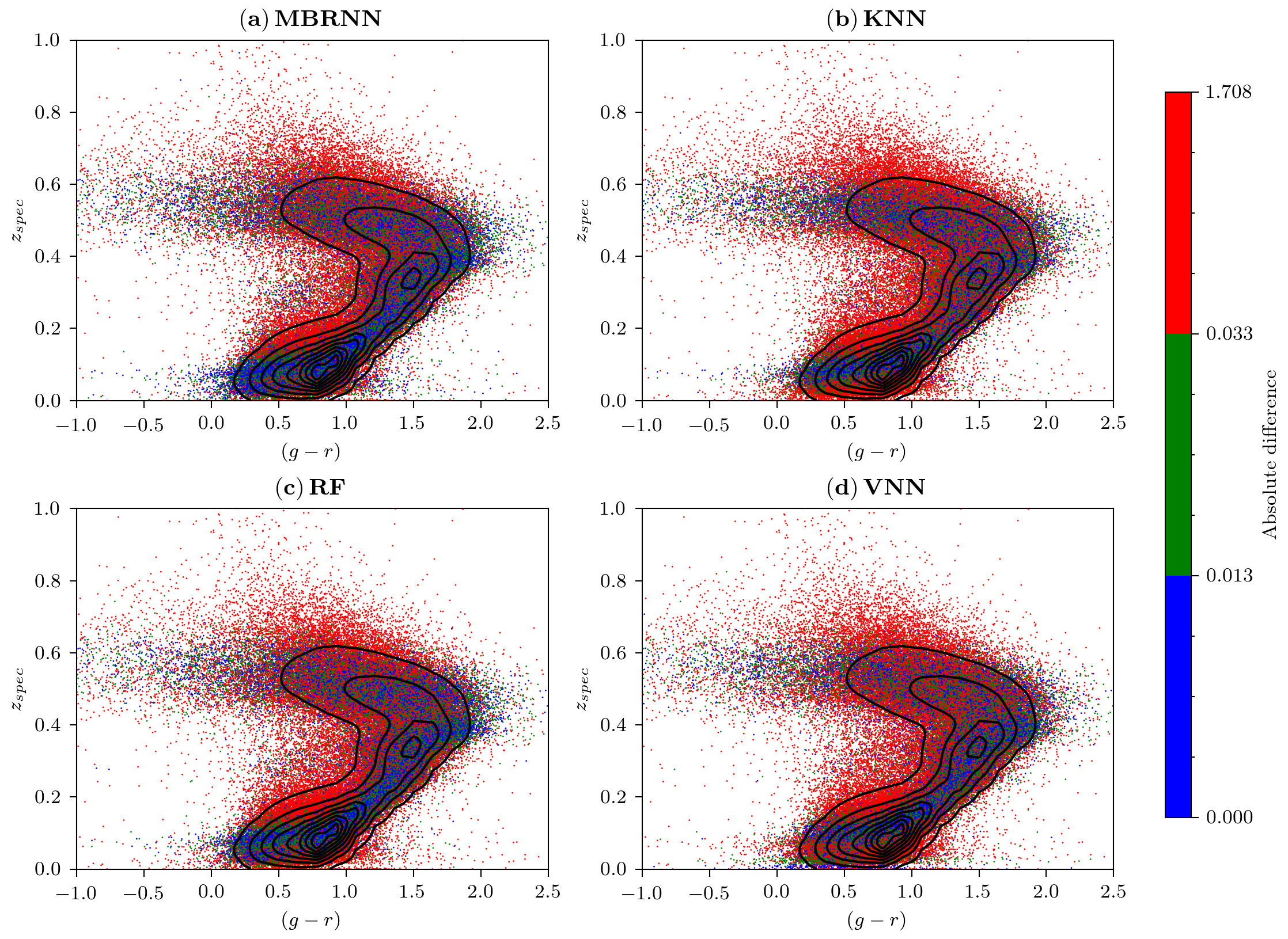
Figure 4: Distribution of the absolute difference between spectroscopic and photometric redshifts in the space of $(g-r)$ in Kron measurement and spectroscopic redshifts. The contour lines show the densities of the samples in this space. We assign samples to low-, middle-, and high-difference groups, and the samples in each group are represented in different colors. Providing the smallest area of the high-difference region in the MBRNN model compared with the other baseline models, the MBRNN model reproduces spectroscopic redshifts with the highest accuracy in the outskirt area of the contours.

Figure 5: Left: Distribution of the difference between the average and mode photometric redshifts for the cat and non-cat cases. Right: Distribution of the confidence estimation for photometric redshifts. The vertical solid and dashed lines mark the mean confidence and accuracy, respectively, for each case.

Table 2: Metrics comparison between the average and mode point estimation of the MBRNN and baseline models. The best performing cases in each search are presented in boldface.

Model	Bias	MAD	$\sigma$	$\sigma_{68}$	NMAD	$R_{cat}$
MBRNN (mode)	0.0036	0.0266	0.0430	0.0274	0.0256	0.0111
MBRNN (avg)	0.0017	0.0254	0.0394	0.0272	0.0256	0.0084
KNN	0.0055	0.0324	0.0487	0.0352	0.0340	0.0158
RF	0.0027	0.0277	0.0430	0.0294	0.0277	0.0116
VNN	0.0046	0.0307	0.0450	0.0338	0.0327	0.0113

We quantitatively assess and visually inspect photometric redshifts obtained by the MBRNN model using test set samples. The empirically optimal model configuration for inference is selected in the grid search (see appendix A). The default model setup adopts the anchor loss with $\gamma$ of 0 and 64 uniform redshift bins. Henceforth, unless otherwise stated, we shall restrict ourselves to the MBRNN model with this setup.

Because the baseline models perform regression, we require a way to derive the point estimation of redshifts with the MBRNN model for a fair comparison with the baseline models. We first juxtapose the metrics of mode and average photometric redshifts, as shown in Table 2, to determine which estimation is more suitable for point estimation. Average redshifts evince lower metrics than mode redshifts. Because this result indicates that the average estimation accompanies higher point estimation accuracy than the mode estimation, we use average redshifts in the rest of the analysis related to point estimation, except cases specifying the usage of the mode redshift. Using the average estimation of redshifts, we now can equitably compare the MBRNN model with the baseline models.

The MBRNN model shows a higher prediction accuracy for overall redshift ranges than baseline models. Figure 2 shows the distribution of differences between spectroscopic and photometric redshifts in the MBRNN and baseline models. We obtain the distributions of the differences by subtracting the distribution of photometric redshifts from that of spectroscopic redshifts. The MBRNN model’s relatively close-to-zero differences indicate that it best captures the multi-modal behavior of targets, i.e., redshifts. The KNN, RF, and VNN models show poorer descriptions for the heterogeneous property of targets, particularly for redshift ranges with distribution peaks. These results are naively expected from the lowest metrics of the MBRNN model compared with the baseline models as presented in Table 2, even though the metrics, which are marginalized into one scalar throughout multiple dimensions, cannot represent locally different behaviors of the distribution.

The distributions of spectroscopic and photometric redshifts shown in Figure 3 summarize well the differences reported in the metrics. The density peaks of the MBRNN and RF models are aligned with the slope-one line, whereas those of the KNN and VNN models are misaligned. This difference reflects lower deflection-related metrics (i.e., bias and MAD) of the MBRNN and RF models. As expected from the dispersion-related metrics (i.e., $\sigma$ and $\sigma_{68}$), the redshift distribution of the MBRNN model shows the smallest dispersion around the slope-one line. This characteristic is conspicuous in redshift regions with the distribution peaks (i.e., $z_{spec}\sim$ 0.125, 0.35, and 0.5), as presented in Figure 1, where scatters spread more extensively than other redshift regions. The small bias and dispersion values of the MBRNN model contribute to the highest Pearson correlation coefficient.

The lack of objects in the input space is one of the primary causes that induce prediction difficulty. Figure 4 shows the distribution for the absolute difference of redshifts between spectroscopic and photometric redshifts in the space of the input $(g-r)$ in Kron measurement and target redshifts. Although this visualization only shows the projected distribution in the input $(g-r)$ space with degeneracy of the other input features in the higher dimensional space, the $(g-r)$ color has a well known correlation with redshifts, and its interpretation is usually straightforward in examining models (e.g. Korytov et al., 2019). When grouping the samples into low-, middle-, and high-difference groups corresponding to about 33% of the samples per group in the MBRNN model, a large number of samples with significant redshift discrepancy are found independently in models. Intriguingly, the high-difference groups are similarly distributed in every model, whereas the area of the regions corresponding to this group is the smallest in the MBRNN model. These regions are the outskirts of the density contour lines in which the objects sparsely reside. As presented in Appendix B, the distribution of the cat samples in the MBRNN model is similar to that of baseline models. These model-independent patterns also can be found in Figure 2. The results indicate that the samples populating over the specific regions in the input space are likely to bring high prediction difficulty regardless of the model.

The high-difference samples possibly have multi-modal model probability distributions. Benefiting from the MBRNN model’s property as a probabilistic classification model, we examine the distribution of the difference between the average and mode photometric redshifts for the cat and non-cat samples. Figure 5 shows that the cat error samples have higher differences than non-cat ones. The higher differences between the average and mode estimation of the cat samples indicate that the model-estimated probabilities of cat samples are possibly multi-modal.

Furthermore, the confidence distribution of the MBRNN model shown in Figure 5 endorses our interpretation of the cat samples. Confidence expresses a model’s level of certainty about the classification result for a given sample. The measure of confidence is defined as the maximum value in the probability output of a model (Hendrycks & Gimpel, 2017). The low confidence of cat samples indicates a high possibility that these samples have multiple probability peaks.

It is worthwhile to refer to the practical guide for flagging objects that require caution in analysis. In the confidence histogram presented in Figure 5, the difference between mean confidence and accuracy of cat samples is higher than that of non-cat samples. We may refer that the model is well-calibrated for non-cat samples because mean confidence and accuracy are comparable (Guo et al., 2017). However, the model is overconfident about the cat samples because the mean confidence of the model is significantly higher than mean accuracy. In this case, caution is required because overconfident estimation leads to high prediction error and may lead to an incorrect interpretation. We recommend being cautious about objects outside the dense regions in the input space because the model is overconfident about cat samples, and most of the cat samples reside in the low-density region of input space (see Figure 4).

4.2 Ensemble Model Performance Test

Figure 6: Distribution of photometric redshifts in the MBRNN model with 64 uniform bins (left) and 512 non-uniform bins (right) with the anchor loss $\gamma$ of 0, 2, 5, and 8. The distribution of spectroscopic redshifts is also drawn for comparison.

Table 3: The metrics of the ensemble learning. We also summarize the results of the single model for comparison.

Bin type	Case	Bias	MAD	$\sigma$	$\sigma_{68}$	NMAD	$R_{cat}$
64 uniform bins	Single Model	0.0017	0.0254	0.0394	0.0272	0.0256	0.0084
	E1	0.0023	0.0255	0.0393	0.0274	0.0258	0.0084
	E2	0.0019	0.0254	0.0392	0.0273	0.0256	0.0083
	E3	0.0010	0.0253	0.0389	0.0272	0.0255	0.0082
	E4	0.0020	0.0255	0.0394	0.0273	0.0257	0.0086
512 non-uniform bins	Single Model	0.0023	0.0256	0.0404	0.0272	0.0255	0.0090
	E1	0.0021	0.0255	0.0400	0.0272	0.0255	0.0088
	E2	0.0021	0.0255	0.0400	0.0272	0.0255	0.0088
	E3	0.0021	0.0255	0.0400	0.0272	0.0255	0.0087
	E4	0.0022	0.0256	0.0405	0.0272	0.0255	0.0090

Performance elevation of the integrated model through ensemble learning emerges from diverse specialties of individual models. During grid-search, we find that the anchor loss assigns different specialties to models based on $\gamma$. As the value of $\gamma$ increases, the distributions of photometric redshifts shift toward the higher redshift region in the uniform bin case (see Figure 6). Because the loss with larger $\gamma$ allocates more difficult objects for prediction with bigger weights, this model bias is attributed to the higher redshift region which corresponds to the most difficult part for prediction from the model’s perspective .

We examine four ensemble methods explained in Section 3. Because the models with high anchor loss $\gamma$ focus excessively on the high redshift region, we perform ensemble learning with models trained with moderate values of $\gamma$: 0, 0.2, 0.5, and 1. Furthermore, for comparison, we test ensemble methods with 512 non-uniform bins trained with the same set of $\gamma$ values. A set of models used for each ensemble combination has the same architecture and number of redshift bins. The ensemble experiments with different numbers of bins and sets of $\gamma$ values can be found in Appendix C.

We report that E3 with 64 uniform bins has the best performance metrics. Moreover, the E3 ensemble model is well-calibrated. Appendix D provides the calibration study of the ensemble model. In other words, E3 successfully considers the varied specialties of the individual models with different values of $\gamma$. Table 3 compares the results of the four different ensemble methods using 64 uniform bins and 512 non-uniform bins.

For the 512 non-uniform bin cases, all methods outperform the single model; however, the performance disparity between the ensemble methods is not as pronounced as it is in the uniform bin case. We recognize that it is because improvement is attributed to the stochastic differences between models, and not diverse specialties. The non-uniform bins are designed to make each bin have an almost uniform number of samples. Since the prediction difficulty mostly stems from the scarcity of data, the non-uniform bin cases have no particularly challenging parts to predict. Therefore, it results in monotonous specialties of individual models being insensitive to the variation of $\gamma$. Figure 6 shows that the redshift distributions in the MBRNN model with the non-uniform bins do not vary significantly as the $\gamma$ increases. Consequently, it results in a small improvement in all ensemble methods because of the stochastic difference among the single models.

Figure 7: Redshift distribution of the comparison samples for model validation as summarized in Table 4. The plot displays redshifts up to approximately 1 even though the maximum redshift is 4.15 in the HSC-PDR2-Mizuki-NonGalaxy.

Table 4: Comparison data with either spectroscopic or photometric redshifts.

Name	Number of objects	Maximum redshift	Reference
HeCS	20,544	0.72	Rines et al. (2013)
SDSS-DR12-LPSC	38,818	1.00	https://www.sdss.org/dr12/algorithms/photo-z/
HSC-PDR2-Mizuki-Galaxy	6,996	1.47	Nishizawa et al. (2020)
HSC-PDR2-Mizuki-NonGalaxy	3,267	4.15

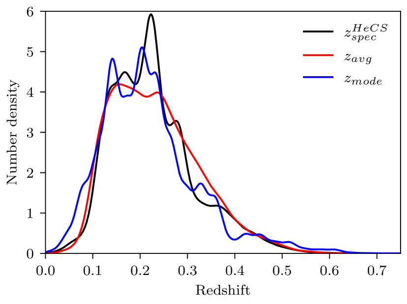
Figure 8: Left: Distribution of the comparison HeCS spectroscopic redshifts and derived photometric redshifts $z_{avg}$ as the average value, and $z_{mode}$ as the mode value. Right: The distribution of the absolute difference between the HeCS spectroscopic redshifts and the derived $z_{avg}$ in the space of $(g-r)$ and HeCS spectroscopic redshifts. Following Figure 4, the samples are color-coded, and the distribution of the training samples is drawn as contour lines for comparison. The distribution of the absolute difference between $z_{spec}$ and $z_{avg}$ with respect to $(g-r)$ in Kron measurement evidently shows that the incorrect estimation of $z_{avg}$ is due to the lack of sufficient training samples to occupy the input space.

5 Model Validation

We compare our photometric redshift results with other existing spectroscopic or photometric redshifts from various sources to investigate when the trained models fail or are not trustworthy. In particular, the data collected from the OOD with respect to the training data distribution should have highly uncertain photometric redshifts because the training data have never allowed the model to acquire the relevant information about the OOD data (e.g., Ren et al., 2019). Table 4 summarizes the comparison data, and Figure 7 shows the redshift distribution of the comparison samples. We match the PS1 DR1 data to comparison data with a search radius of 0.5″, and we apply the same selection and filtering rules to the PS1 DR1 data as we do to the training samples.

5.1 Validation with Spectroscopic Redshift Samples

We estimate the photometric redshifts of the matched PS1 DR1 objects for the dataset HeCS. The HeCS dataset includes objects with the spectroscopic redshifts of galaxies found in galaxy cluster areas over z = 0.1 – 0.3 (Rines et al., 2013). Therefore, this dataset contains both cluster members and line-of-sight field galaxies. We use objects with a redshift quality flag of Q, thus indicating a secure redshift. Moreover, we exclude objects with redshifts $<$ 0.009 because they are not galaxies generally.

The comparison with spectroscopic samples allows us to unbiasedly evaluate the performance of our trained machine learning model although the comparison sample size is not as large as that of training samples. As shown in Figure 7, the true redshift range is well matched to the redshift range over which we intend to use the trained model. However, the distribution of true redshifts differs from that of training samples. Moreover, this comparison helps us assess how well the trained model can be used in identifying potential galaxy groups and clusters with the PS1 DR1 data (see Euclid Collaboration et al., 2019, for discussion).

As shown in Figure 8, the photometric redshifts are well estimated for the redshift range of the HeCS dataset. However, we find that certain objects with the biased estimation of photometric redshifts over 0.1 $<~{}z~{}<$ 0.3. As the distribution of the absolute difference between the spectroscopic and photometric redshifts in the space of $(g-r)$ and the spectroscopic redshifts highlights, the biased estimation of the photometric redshifts is attributed to the lack of blue training samples for given redshifts over 0.1 $<~{}z~{}<$ 0.3. Although the distribution in the input space such as $(g-r)$ does not completely show the distribution mismatch with respect to the model because of the model’s nonlinearity, the mismatched training and test HeCS distributions lead to the model’s biased results. This result indicates that our model may require to be updated with sufficient samples of blue galaxies to estimate photometric redshifts in galaxy groups and clusters over 0.1 $<~{}z~{}<$ 0.3.

5.2 Validation with Photometric Redshift Samples

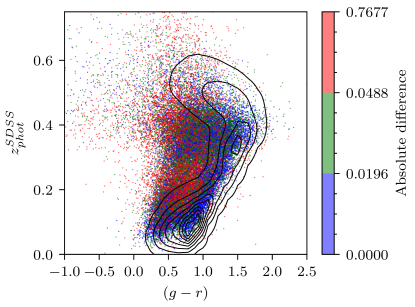
Figure 9: Left: Distribution of the comparison SDSS photometric redshifts and derived photometric redshifts $z_{avg}$ for the PS1 photometric data. Right: The distribution of the absolute difference between SDSS photometric redshifts and the derived $z_{avg}$ in the space of $(g-r)$ (Kron measurement) and SDSS photometric redshifts. The scatters are color-coded, as in Figure 8, and the distribution of PS1 training samples are drawn as contour lines for comparison. The distribution of the absolute difference between SDSS photometric redshifts and the derived $z_{avg}$ with respect to $(g-r)$ shows that the significant fraction of samples with a large difference of photometric redshifts have $(g-r)$ out of the main training samples. However, we still find some consistent estimation of photometric redshifts between the two different methods/data for $(g-r)\sim 0.7$ and $z_{phot}^{SDSS}\sim 0.3$.

Our trained model is compared with other photometric redshift estimation methods. Because there are more galaxy objects with known photometric redshifts than those with spectroscopic redshifts, we intend to use this comparison to assess the validity of the trained model over a wide range of redshifts and input space although photometric redshifts are not as precise and accurate as spectroscopic redshifts.

As summarized in Table 4, we use the SDSS Data Release 12 (DR12) (Alam et al., 2015), which contains photometric redshifts derived from a nearest-neighbor fit with a kd-tree structure of training samples (Csabai et al., 2007). We extract SDSS photometric redshifts for objects found in the area centered at RA 26.25°, DEC -7.5°with a radius of 2.5°, and we extract the PS1 DR1 objects corresponding to the SDSS objects that were identified. After discarding objects with SDSS spectroscopic redshifts, the sample size becomes 44,890 for the same filtering rule that we use for the training data of the PS1 DR1 data. We examine point-source scores of the 44,890 objects in the PS1 DR1 catalog (Tachibana & Miller, 2018), leaving out only extended sources (i.e., galaxies) in the PS1 image data with the condition of the point-source score $<$ 0.1. The filtered data, including 38,818 objects commonly found in the SDSS and PS1, should comprise only galaxy-like objects for which our trained model should be able to estimate photometric redshifts.

Generally, two different estimations of photometric redshifts are consistent although the methods and training data are completely different. Figure 9 shows the comparison between the two photometric redshift inferences where $z_{phot}^{PS1}$ corresponds to $z_{avg}$ in our estimation and $z_{phot}^{SDSS}$ represents estimation by robust fit to nearest neighbors in the SDSS reference set. Pearson’s correlation coefficient $\rho\sim 0.81$ confirms that the two methods are consistent for most samples. A dominant fraction of objects with discrepant redshifts seems to have a range of colors not properly represented by training samples; however, we report certain fraction of objects to have consistent redshifts although their colors do not follow the color of the training samples (see Figure 9).

We examine possible causes of certain objects showing a large discrepancy in the estimated redshifts. For example, SDSS J014232.69-090324.5 (catalog ) corresponding to PS1 DR1 objid $=$ 97130256361222090 seems blended in the PS1 DR1 and the SDSS images. The photometric redshifts of this object are 0.203 and 0.858 as $z_{phot}^{SDSS}$ and $z_{phot}^{PS1}$, respectively. The SDSS J014228.47-072343.0 (catalog ) (i.e., PS1 DR1 objid $=$ 99120256186386095) shows possible effects of blending in their images with the photometric redshifts $z_{phot}^{SDSS}=0.018$ and $z_{phot}^{PS1}=0.391$. The blending of sources is a well-known problem for estimating photometric redshifts (Jones & Heavens, 2019; LSST Dark Energy Science Collaboration et al.(2021)LSST Dark Energy Science Collaboration (LSST DESC), Abolfathi, Alonso, Armstrong, Aubourg, Awan, Babuji, Bauer, Bean, Beckett, Biswas, Bogart, Boutigny, Chard, Chiang, Claver, Cohen-Tanugi, Combet, Connolly, Daniel, Digel, Drlica-Wagner, Dubois, Gangler, Gawiser, Glanzman, Gris, Habib, Hearin, Heitmann, Hernandez, Hložek, Hollowed, Ishak, Ivezić, Jarvis, Jha, Kahn, Kalmbach, Kelly, Kovacs, Korytov, Krughoff, Lage, Lanusse, Larsen, Le Guillou, Li, Longley, Lupton, Mandelbaum, Mao, Marshall, Meyers, Moniez, Morrison, Nomerotski, O’Connor, Park, Park, Peloton, Perrefort, Perry, Plaszczynski, Pope, Rasmussen, Reil, Roodman, Rykoff, Sánchez, Schmidt, Scolnic, Stubbs, Tyson, Uram, Villarreal, Walter, Wiesner, Wood-Vasey, & Zuntz, LSST DESC). We also find certain objects have conflicting colors between the SDSS DR12 and PS1 DR1 catalogs. For example, SDSS J014126.01-065056.2 (catalog ) matched to the PS1 DR1 objid $=$ 99780253584271692 has $(g-r)=1.1\pm 0.01$ (Kron color) and $0.7\pm 0.32$ (aperture color) in the SDSS DR12 and PS1 DR1 catalogs, respectively. The photometric redshifts of this object are $z_{phot}^{SDSS}=0.941$ and $z_{phot}^{PS1}=0.172$.

5.3 Model Outcomes for Non-galaxy Objects

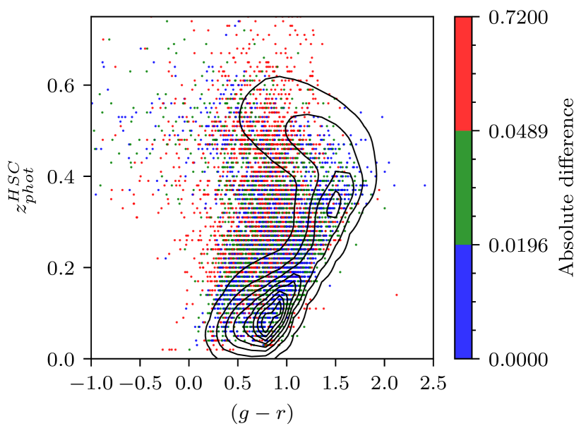
Figure 10: Left: Distribution of the comparison HSC galaxy photometric redshifts and derived photometric redshifts $z_{avg}$ for the PS1 photometric data. Right: The distribution of the absolute difference between the HSC photometric redshifts and the derived $z_{avg}$ in the space of $(g-r)$ (Kron measurement) and HSC photometric redshifts. The color-coding of scatters and contour lines are as those of Figure 9. The pattern of the discrete $z_{phot}^{HSC}$ distribution appears clearly in both plots. The correlation $\rho$ between the two photometric redshifts is lower than that in for the comparison with the SDSS photometric redshift presented in Figure 9 partly due to the discrete distribution of $z_{phot}^{HSC}$.

The validity of trained machine learning models depends on the assumption that the training and test data follow the same distribution from the learning model’s view. Therefore, when the trained model infers photometric redshifts for objects obtained from the OOD data, the estimation should be highly uncertain and/or inaccurate. We already present the case showing this effect in Section 5.1 for the slightly different distribution of input features for galaxies between training samples and HeCS test data.

The application of the trained model on the datasets HSC-PDR2-Mizuki-Galaxy and HSC-PDR2-Mizuki-NonGalaxy enables us to evaluate the results for the physically OOD objects, i.e., non-galaxy objects. Photometric redshifts in these datasets are results acquired in running a template fitting-code MIZUKI (Tanaka, 2015; Tanaka et al., 2018; Nishizawa et al., 2020). The estimation products have probabilities of being stars, quasars, and galaxies. We select objects with photometric redshifts around RA 31.25°, DEC -2.5°with a radius of 2.5°. Following the filtering criteria used for the training data, we extract 6,996 objects as galaxy objects and 3,267 objects as non-galaxy objects with the PS1 DR1 data. The number of stars is 3,171 among 3,267 non-galaxy objects. Therefore, $\sim$100 objects are classified as quasars in the HSC test data.

The estimated photometric redshifts of galaxy objects in the HSC comparison data are similarly estimated to what our trained model estimates as shown in Figure 10. In general, our machine-learning estimation of photometric redshifts seems consistent with those derived by the template fitting-code. However, we report certain systematic difference patterns such as objects with $z_{phot}^{HSC}\sim 0.6$ for $z_{phot}^{PS1}\sim 0.1$. The discrete distribution of $z_{phot}^{HSC}$ appears to be a systematic pattern embedded in the HSC Mizuki inference of photometric redshifts. As shown in Figures 8 and 9, we report that most objects with a large difference between the two photometric redshifts can be considered OOD samples based on the input data properties (see Figure 10).

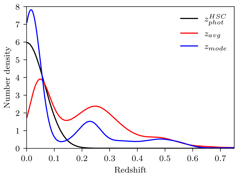
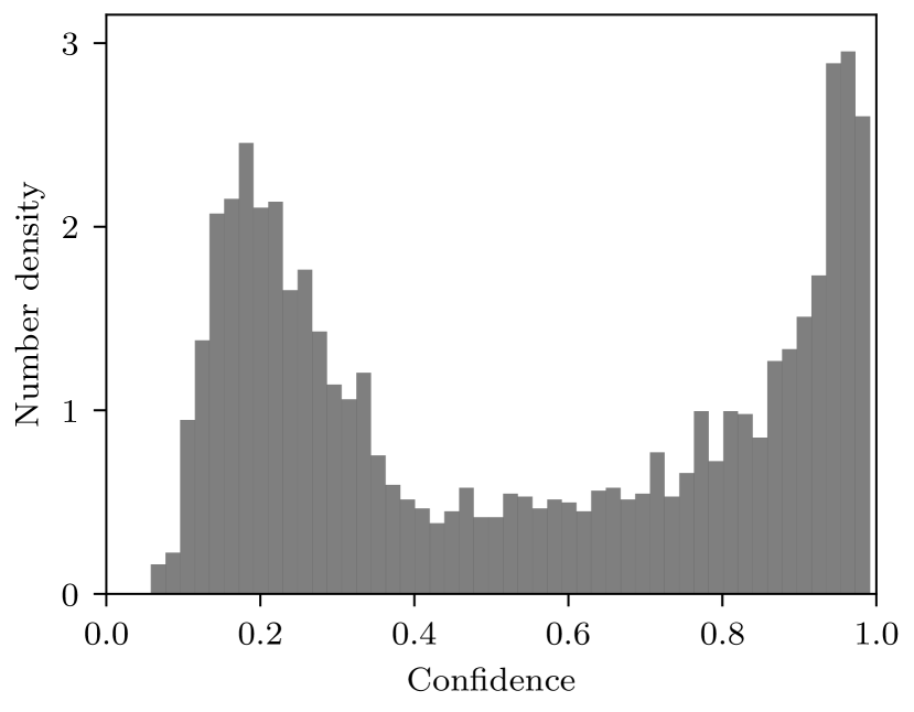
Figure 11: Distribution of the comparison HSC non-galaxy spectroscopic redshifts, derived photometric redshifts $z_{avg}$ as the average value, and $z_{mode}$ as the mode value (left). Confidence distribution of the non-galaxy samples (right) shows that our trained model is overconfident on some of the physically OOD samples.

We examine how our trained model estimates photometric redshifts of non-galaxy objects. If the model is well-trained to inductively infer the galactic photometric redshifts, photometric redshifts of the physically OOD samples (i.e., stars and galaxies) should follow the overall redshift estimation of galaxies when the OOD samples have similar input values as training galaxies. The useful machine learning model should result in a highly uncertain estimation of photometric redshifts for data samples from the OOD with respect to the input space and the trained model even when the OOD samples are galaxies.

Figure 11 shows the distribution of photometric redshifts for the non-galaxy HSC objects. Because the majority of non-galaxy HSC objects are stars, their redshift distribution has a peak at z $=$ 0. Comparing the distribution to that of the training samples (see Figure 7), the derived photometric redshifts of the physically OOD samples share a similar distribution to that of the training samples at z $\sim$ 0.1 and 0.5. However, the derived photometric redshifts of the physically OOD samples show a concentrated distribution around z $=$ 0.25 where the input values and photometric redshifts of these physically OOD samples are distributed in a manner similar to the galaxy OOD samples as shown in Figure 10 (i.e., the galaxy OOD objects at $(g-r)\sim 0.7$ and $z_{phot}^{HSC}\sim 0.25$).

As shown in Figure 11, the trained model produces overconfident results on certain physically OOD samples. We anticipate that the well-trained model will output nearly identical probability distributions for OOD samples as random guesses, i.e., uniform distribution. In such a case, the confidence distribution should be nearly uni-modal with a peak in the low confidence range and then monotonically diminish as the confidence increases. However, the confidence distribution of physically OOD samples is multi-modal and has the tallest peak with high confidence. Therefore, the high confidence of the trained model’s outputs does not guarantee that the tested sample has the same distribution as the training samples, particularly for the physically OOD samples. Unless the physically OOD samples such as stars and quasars are separately classified (e.g., Fotopoulou & Paltani, 2018), the application of our model to these OOD samples can produce incorrect inference results with overconfidence.

6 Discussion and Conclusion

The machine learning model presented in this study shows that 1) the machine-learning estimation of photometric redshifts can incorporate the uncertainty of color measurements and $E(B-V)$ as input data, 2) the anchor loss adopted in the framework of NNs can be useful to handle difficult training data for target prediction generally linked to the sample imbalance problem, thereby improving the trained model for the difficult problem domains, and 3) the ensemble learning approach with various anchor loss weighting parameters is an effective way of maintaining the balance between the increased bias caused by the anchor loss and the improved overall accuracy.

We expect other researchers to use our trained model in various ways with the publicly available Python code on GitHub under an MIT License (Lee & Shin, 2021), which is based on PyTorch (Paszke et al., 2019). The code can be used for both training new data such as the PS1 data release 2 with photometric colors in different types like aperture magnitudes and inference of photometric redshifts with the PS1 DR1 data. As planned, the inference made by our model can be combined with the conventional fitting-based inference. Users of our model can consider using the time-consuming model-fitting codes to estimate the photometric redshifts only for objects with low confidence values or a large difference between $z_{avg}$ and $z_{mode}$ in our machine learning inference (see Figure 5). The model can be adopted and retrained with new training samples, which focus on specific science goals such as studies of low-z red galaxies (e.g., Abdalla et al., 2011). In particular, retraining the model with more fine redshift bins than those used in our study at low redshift might be useful for science goals related to low-redshift galaxies with better performance (i.e., higher accuracy and lower variance).

Our application of ensemble learning and comparison to the other machine learning method results encourages others to combine their machine learning model results with ours in different ensemble learning forms (for example, dynamical ensemble, instead of the static ensemble adopted in this study). As shown in Section 5.2, the consensus between our model and other machine learning models indicates that combining multiple model results, which are generated by either different data or methods, can be a useful approach to improve the reliability of machine learning inference (e.g. Shin et al., 2018).

The performance of ensembling models with the anchor loss with respect to the given redshift bins hints that it might be powerful to combine models trained with the observed spectroscopic training samples, which are mainly low-redshift bright objects, and models trained with the simulated high-redshift or faint training samples. Using the simulated mock catalog data in the machine learning models is not a new concept, and the application of the NNs with the mock data has already been presented in the past (e.g. Firth et al., 2003). Because the observed training samples have the redshift-dependent distribution biased toward low-redshift space (see Figure 1), the lack of high-redshift learning samples can be handled by incorporating high-redshift mock/simulated data if the simulated data is well-calibrated to the observed/expected properties (particularly, photometric properties) of galaxies at high redshifts with a correct distribution of the properties (Sawicki et al., 1997; Kalmbach & Connolly, 2017). Our method can naturally combine the multiple models with redshift bins where a fraction of models trained with mock data perform well for a limited range of redshift bins.

Our examination of the trained model’s limitations leads us to issues that should be addressed to improve machine learning inference of photometric redshifts. First, additional spectroscopic samples are required to improve the trained model’s accuracy. The accuracy of machine learning inference might be degraded for specific parts of mapping between the input and redshift space because of the lack of sufficient training samples, which are generally considered close to OOD samples (Beck et al., 2017). The mismatch between the training sample and test data distributions results in biased estimation of photometric redshifts (Rivera et al., 2018). Even when the test data contain only galaxies, the distribution of input features in the test data can become the OOD case, as we examined in Section 5.1. Therefore, new machine learning models require to include additional spectroscopic samples as training data covering large input and output (i.e., redshift) spaces.

The physically OOD objects become problematic as well as reported in Section 5.3. Some fraction of physically OOD objects can be seen as valid in-distribution galaxies with respect to input space and models even though quasars and stars are physically different from galaxies. Therefore, the algorithm detecting the OOD samples in terms of the input-output mapping cannot handle the physically OOD samples with valid input values. The most straightforward solution to address this issue might be using a separate machine learning model to classify test objects (e.g., Kim et al., 2015; Clarke et al., 2020; Golob et al., 2021) and forward only galaxy objects to the trained model for the inference of photometric redshifts.

Future studies, including our next study, will require to tackle the OOD problem. In particular, the improved model should be able to produce a quantitative evaluation of how much the test objects deviate from the in-distribution samples. The quantitative OOD score of test samples will allow us to use computationally expensive procedures such as spectral modeling for only objects with high OOD scores.

Appendix A Search for the Optimal Configuration of the MBRNN Model

Table A.1: Metrics of the grid search for the best model configuration of the MBRNN model. As mentioned in Section 4, the lower metrics indicate a higher accuracy of the model.

Data scaling	Color uncertainties	$E(B-V)$	Bias	MAD	$\sigma$	$\sigma_{68}$	NMAD	$R_{cat}$
Min-max	Yes	Yes	0.0019	0.0256	0.0398	0.0273	0.0256	0.0088
		No	0.0021	0.0267	0.0412	0.0287	0.0270	0.0096
	No	Yes	0.0028	0.0316	0.0496	0.0329	0.0310	0.0188
		No	0.0030	0.0336	0.0533	0.0346	0.0327	0.0226
Standardization	Yes	Yes	0.0022	0.0256	0.0399	0.0273	0.0257	0.0086
		No	0.0023	0.0268	0.0415	0.0288	0.0270	0.0095
	No	Yes	0.0030	0.0317	0.0498	0.0329	0.0310	0.0191
		No	0.0031	0.0336	0.0535	0.0346	0.0328	0.0229

(a) Metrics for different data scaling methods, and the existence of color uncertainties and $E(B-V)$ as input features.

Loss configuration		Bias	MAD	$\sigma$	$\sigma_{68}$	NMAD	$R_{cat}$
Binary Cross Entropy ($\gamma=0$)		0.0019	0.0256	0.0398	0.0273	0.0256	0.0088
Anchor Loss	$\gamma=0.2$	0.0025	0.0257	0.0398	0.0275	0.0259	0.0087
	$\gamma=0.5$	0.0027	0.0256	0.0396	0.0274	0.0258	0.0086
	$\gamma=1$	0.0027	0.0256	0.0396	0.0275	0.0260	0.0086
	$\gamma=2$	0.0039	0.0260	0.0399	0.0280	0.0266	0.0087
	$\gamma=5$	0.0327	0.0483	0.0611	0.0536	0.0507	0.0451

(b) Metrics for different anchor loss $\gamma$ values.

Bin type		Bias	MAD	$\sigma$	$\sigma_{68}$	NMAD	$R_{cat}$
Uniform Bins	32	0.0020	0.0257	0.0399	0.0274	0.026	0.0086
	64	0.0017	0.0254	0.0394	0.0272	0.0256	0.0084
	128	0.0019	0.0256	0.0398	0.0273	0.0256	0.0088
	256	0.0024	0.0254	0.0396	0.0272	0.0255	0.0084
	512	0.0024	0.0255	0.0396	0.0273	0.0256	0.0086
Non-uniform Bins	32	0.0144	0.0337	0.0577	0.0310	0.0281	0.0342
	64	0.0075	0.0285	0.0470	0.0288	0.0266	0.0168
	128	0.0045	0.0266	0.0429	0.0278	0.0259	0.0117
	256	0.0028	0.0259	0.0415	0.0274	0.0255	0.0096
	512	0.0023	0.0256	0.0404	0.0272	0.0255	0.0090

(c) Metrics for different redshift bin configurations.

We perform a grid search by varying model configurations with the validation data to find the empirically optimal configuration of the MBRNN model. The grid search includes three different sets of configuration variations. First, when setting the number of redshift bins to 128 and using the anchor loss with $\gamma~{}=~{}0$, we examine the changes in the model’s accuracy in terms of input data scaling methods (i.e., standardization vs. min-max normalization), and the existence of color uncertainties and $E(B-V)$ as input features.

The model using the min-max normalization, color uncertainties, and $E(B-V)$ shows the best point-estimation accuracy as summarized in Table 1(c) (a). Including the color uncertainties as input features has the largest impact on point-estimation accuracy among three factors. The min-max normalization and inclusion of $E(B-V)$ in the input have small positive effects on point-estimation accuracy.

Second, we perform the grid-search for the anchor loss parameter $\gamma$ fixing the number of redshift bins to 128. Because the anchor loss requires a prior setup of $\gamma$ before training, we examine a set of $\gamma$ values of 0 (i.e., binary cross entropy loss), 0.2, 0.5, 1, 2, and 5. The results of this second grid search are presented in Table 1(c) (b). The model with $\gamma$ of 0 outperforms the others in terms of the overall accuracy as naively expected.

Using the maximum performance configuration, we finally examine the various strategies of redshift binning and the number of bins. The search includes a comparison of results between uniform and non-uniform binning methods as well as the results for the 32, 64, 128, 256, and 512 redshift bins. In the non-uniform redshift binning, we set the bin edges such that each bin contains nearly the same number of samples, as explained in Section 3.2. As illustrated in Table 1(c) (c), the MBRNN model with 64 uniform bins outperforms the other configurations for most metrics, although the difference is not significant. Moreover, we discover that the uniform binning case outperforms the non-uniform one.

Appendix B Catastrophic Samples

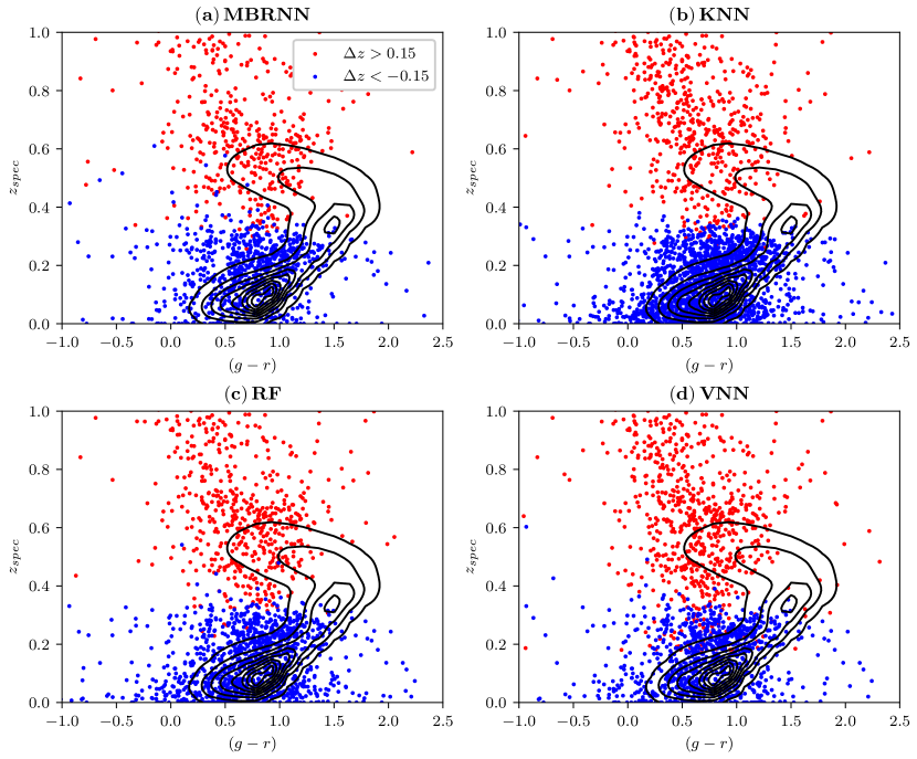
Figure B.1: Distributions of the cat samples in the space of $(g-r)$ in Kron measurement and spectroscopic redshifts. The cat samples are shown with different colors for $\Delta z>0.15$ (red) and $\Delta z<-0.15$ (blue). The lower fraction of the cat samples in the MBRNN than in other models is mainly due to the reduction of these samples at low redshifts.

We examine the distributions of the cat samples in the input space according to models and find that these samples populate in the similar regions of the input space. Figure B.1 presents the distributions of under and overestimated cat samples in the MBRNN and baseline models. As shown in the figure, the point-estimated photometric redshifts of the cat samples in MBRNN with true spectroscopic redshifts larger and lower than $z_{spec}\sim 0.4$ tend to be under- and over-estimated, respectively. This pattern appears in the other baseline models too, and the under- and over-estimated photometric redshifts of the cat samples are similarly distributed in the input space. However, the area taken by the cat samples in the MBRNN model is smallest among the models, being consistent with the fact that the $R_{cat}$ is smallest in the MBRNN model (see Table 2).

We also find that MBRNN works better than the baseline models particularly in the low redshift range. Specifically, we compare how many cat samples found in the RF model, which shows the best performance among the baseline models, become non-cat samples in the MBRNN model. The RF model has 766 cat samples in its test, and the entire 543 and 223 samples with over- and under-estimated photometric redshifts in the RF model are the non-cat samples in the MBRNN. Especially, samples with $z_{spec}\sim 0$ mainly turn into the non-cat objects in the MBRNN model (see Figure B.1).

The cat samples in the models include various cases. When inspecting the cat samples in the MBRNN model, we find that some objects such as SDSS J014904.18+243502.4 (catalog ), SDSS J104307.62+084059.2 (catalog ), and SDSS J101223.88+161313.4 (catalog ) might not have reliable photometric input features due to neighbor objects. Star-forming galaxies with emission lines are also found as the cat samples. For example, SDSS J085139.46+455518.4 (catalog ) and SDSS J091022.97+164534.9 (catalog ) have emission-lines representing star formation at redshifts of 0.28 and 0.30, respectively. Objects like SDSS J150912.92+344418.1 (catalog ) at $z_{spec}~{}=~{}0.06028$ have a large apparent size, and their photometry might not be reliable.

Appendix C Results With Different Ensemble Learning Configurations

Table C.2: Metrics for the ensemble cases with different redshift bins.

Number of bins	Bias	MAD	$\sigma$	$\sigma_{68}$	NMAD	$R_{cat}$
32	0.0015	0.0255	0.0392	0.0274	0.0260	0.0084
64	0.0010	0.0253	0.0389	0.0272	0.0255	0.0082
128	0.0014	0.0254	0.0390	0.0272	0.0256	0.0082
64 & 128	0.0013	0.0253	0.0389	0.0272	0.0255	0.0083

Furthermore, we present the performance of the E3 ensemble model with 32 and 128 uniform redshift bins as well as the results obtained from the runs of the adopted 64 bins. Moreover, we consider merging the single models trained with 64 and 128 redshift bins rather than only the results with the same number of redshift bins. In particular, four single models sharing the same number of bins and trained with different anchor loss $\gamma$s — 0, 0.2, 0.5, and 1 — are combined for the ensemble models of 32, 64, and 128 bins, respectively. For the merged ensemble model of 64 and 128 bins, however, eight single models are combined; four each of the 64 and 128 bin models trained with different $\gamma$ values. Merging the models with the different number of redshift bins is conducted by interpolating their probability outputs to a higher number of redshift bins while maintaining the probability sum equal to 1.

Table C.2 compares the point estimation metrics of the ensemble models with 32, 64, and 128 bins, and the case of combining models generated with 64 and 128 redshift bins. We find no advantage or improvement in these cases over the adopted ensemble model of combing the runs with 64 redshift bins.

Table C.3: Metrics for ensembling cases with the different anchor loss $\gamma$ values. The set ${\cal{G}}$ contains the models trained with anchor loss $\gamma$ of 0, 0.2, 0.5, and 1.

Set of $\gamma$	Bias	MAD	$\sigma$	$\sigma_{68}$	NMAD	$R_{cat}$
${\cal{G}}$	0.0010	0.0253	0.0389	0.0272	0.0255	0.0082
${\cal{G}}\cup\{2\}$	0.0014	0.0253	0.0389	0.0272	0.0256	0.0083
${\cal{G}}\cup\{2,5\}$	0.0024	0.0255	0.0389	0.0274	0.0260	0.0082
${\cal{G}}\cup\{2,5,8\}$	0.0040	0.0258	0.0389	0.0279	0.0268	0.0083

Moreover, we check how the high $\gamma$ values of the anchor loss affect the performance of the ensemble model. We attempt the E3 ensemble method with 64 uniform redshift bins while combining the additional results with $\gamma$ in the order of 2, 5, and 8 into the set of models used in the adopted E3 model (${\cal{G}}$), which is described in Section 4.2 as the model combining the results with $\gamma~{}=~{}0,0.2,0.5,$ and $1$. Table C.3 illustrates the metrics of the models for the trial configurations. Compared with the other runs, the ensemble model with the set ${\cal{G}}$ achieves the highest accuracy in general.

Appendix D Examination of The Ensemble Model Calibration

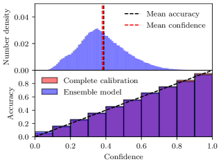
Figure D.2: Top: Confidence distribution in the E3 model. Black and red vertical lines indicate the mean accuracy and confidence of the E3 model. Bottom: Reliability diagrams of the E3 model. Red and blue bars represent the distribution of the complete calibration and the E3 model result, respectively. The black dashed line marks a line with a slope of 1, meaning the perfect calibration.

Many typical modern NNs are not well-calibrated (Guo et al., 2017). Hence, we examine the calibration of our E3 ensemble model. A well-calibrated model should have similar mean accuracy and confidence values. Figure D.2 shows that our ensemble model E3 is well-calibrated. The difference between the mean accuracy and confidence of our E3 ensemble model is $\sim$0.0078, which is close to 0. A reliability diagram depicting the accuracy variation as per the confidence confirms the adequate calibration of the ensemble model, almost identical to the completely calibrated case.

Appendix E Effects of The Galactic Extinction Correction

We apply the galactic extinction correction to the input colors using $E(B-V)$ and a simple correction rule, and then we train our model with corrected colors. Therefore, the model learns without $E(B-V)$ as a training input feature in this experiment. Three different correction rules are tested with the given $E(B-V)$, and the three different correction results (I, II, and III cases in Table E.4) are compared in terms of model performances. Case I adopts the correction given as equations (7) to (13) in Tonry et al. (2012) with the observed apparent $(g-i)$ color. We note that this correction is fundamentally incorrect because the correction is valid only with the intrinsic color $(g-i)$, which we do not know beforehand, rather than the observed color (see Galametz et al., 2017, for discussions). The correction in cases II and III do not depend on $(g-i)$. Their correction rules adopt the representative values of the extinction $A$ given as $A$ at the pivot in Galametz et al. (2017) and $A$ values used in Schindler et al. (2019) for cases II and III, respectively. Although the metrics in case II are the lowest overall, there are no significant differences among these three cases.

In case II, we analyze the effect of the correction on the photometric redshifts inferred by the trained model. We split $E(B-V)$ values into three different ranges, and each range has $\sim$33% of samples as low, middle, and high $E(B-V)$ values. Then, we compare photometric redshifts derived from our main model trained with $E(B-V)$ as an input feature ($z_{model}$) with case II results acquired with the extinction-corrected color data ($z_{comp}$). The left panel of Figure E.3 shows that the redshift difference ($\Delta z~{}=~{}z_{model}~{}-~{}z_{comp}$) distribution. Interestingly, the distributions of redshifts for the low and high $E(B-V)$ values are positively and negatively shifted from a non-bias line ($\Delta z=0$), respectively. This pattern is conspicuous in the right panel of the figure, which shows a comparison between $z_{comp}$ and $z_{model}$. These results indicate that the model trained with the extinction-corrected colors tends to under- and over-estimate redshifts compared to $z_{model}$ for low and high $E(B-V)$ objects, respectively, indicating that the systematic bias is induced by the Galactic extinction correction on colors.

Figure E.4 shows the distribution of the $z_{spec}-z_{model}$ and $z_{spec}-z_{comp}$, where $z_{spec}$ corresponds to true spectroscopic redshifts. The distribution reported in the model with $E(B-V)$ as input features does not vary with respect to $E(B-V)$. However, the distribution of $z_{spec}-z_{comp}$ reveals that the trend found in Figure E.3 can be explained by the fact that the extinction correction introduces bias into the redshift inference.

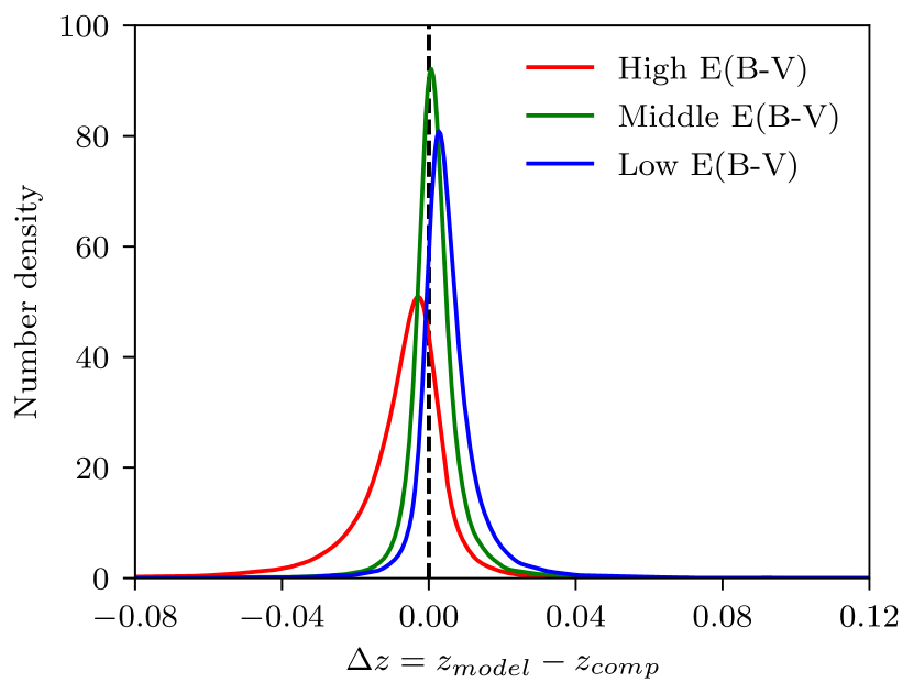
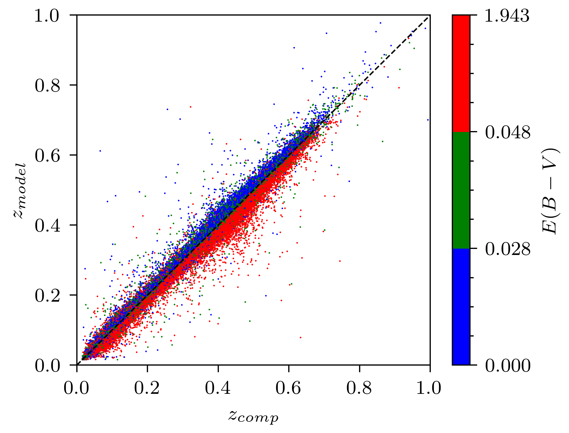
Figure E.3: Distribution of the difference between photometric redshifts ($z_{model}$) from the model trained with $E(B-V)$ and those ($z_{comp}$) from the model trained without $E(B-V)$ but with the Galactic extinction-corrected colors (left). The samples are grouped into the low, medium, and high $E(B-V)$ value groups in which each group has approximately one-third of the number of samples. $\Delta z$ shows systematic differences depending on the $E(B-V)$ values. This pattern is also found in the redshift comparison plot (right). The redshifts of the low and high $E(B-V)$ samples are mostly in the under- and over-estimation regions with respect to the correspondence line, which is represented by the dashed line, respectively.

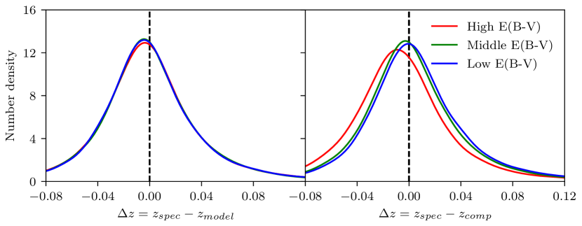
Figure E.4: Distributions of the difference between spectroscopic redshift ($z_{spec}$) and photometric redshifts ($z_{model}$ and $z_{comp}$). The samples are binned with respect to $E(B-V)$ as done for Figure E.3. While the difference distributions for the $z_{model}$ (left) are unbiased regarding $E(B-V)$, the distributions of the $z_{comp}$ with higher $E(B-V)$ are shifted towards the lower $\Delta z$ direction (right).

Table E.4: Metrics for the experiments with three different Galactic extinction correction methods.

Case	Bias	MAD	$\sigma$	$\sigma_{68}$	NMAD	$R_{cat}$
I	0.0019	0.0261	0.0403	0.0280	0.0265	0.0090
II	0.0019	0.0261	0.0404	0.0280	0.0264	0.0089
III	0.0019	0.0262	0.0405	0.0281	0.0265	0.0092

References

- Abdalla et al. (2011) Abdalla, F. B., Banerji, M., Lahav, O., & Rashkov, V. 2011, MNRAS, 417, 1891, doi: 10.1111/j.1365-2966.2011.19375.x
- Aguado et al. (2019) Aguado, D. S., Ahumada, R., Almeida, A., et al. 2019, ApJS, 240, 23, doi: 10.3847/1538-4365/aaf651
- Alam et al. (2015) Alam, S., Albareti, F. D., Allende Prieto, C., et al. 2015, ApJS, 219, 12, doi: 10.1088/0067-0049/219/1/12
- Altman (1992) Altman, N. S. 1992, The American Statistician, 46, 175, doi: 10.1080/00031305.1992.10475879
- Amon et al. (2018) Amon, A., Blake, C., Heymans, C., et al. 2018, Monthly Notices of the Royal Astronomical Society, 479, 3422, doi: 10.1093/mnras/sty1624
- Ball et al. (2008) Ball, N. M., Brunner, R. J., Myers, A. D., et al. 2008, The Astrophysical Journal, 683, 12
- Banerji et al. (2008) Banerji, M., Abdalla, F. B., Lahav, O., & Lin, H. 2008, Monthly Notices of the Royal Astronomical Society, 386, 1219, doi: 10.1111/j.1365-2966.2008.13095.x
- Barron (2019) Barron, J. T. 2019, in Proceedings of the IEEE/CVF Conference on Computer Vision and Pattern Recognition (CVPR)
- Beck et al. (2017) Beck, R., Lin, C. A., Ishida, E. E. O., et al. 2017, MNRAS, 468, 4323, doi: 10.1093/mnras/stx687
- Beck et al. (2021) Beck, R., Szapudi, I., Flewelling, H., et al. 2021, MNRAS, 500, 1633, doi: 10.1093/mnras/staa2587
- Bilicki et al. (2018) Bilicki, M., Hoekstra, H., Brown, M., et al. 2018, Astronomy & Astrophysics, 616, A69
- Blake & Bridle (2005) Blake, C., & Bridle, S. 2005, Monthly Notices of the Royal Astronomical Society, 363, 1329, doi: 10.1111/j.1365-2966.2005.09526.x
- Bolzonella et al. (2000) Bolzonella, M., Miralles, J. M., & Pelló, R. 2000, A&A, 363, 476. https://arxiv.org/abs/astro-ph/0003380
- Bottou (2010) Bottou, L. 2010, Large-Scale Machine Learning with Stochastic Gradient Descent, 177–186, doi: 10.1007/978-3-7908-2604-3_16
- Breiman (2001) Breiman, L. 2001, Machine Learning, 45, 5, doi: 10.1023/A:1010933404324
- Brescia et al. (2013) Brescia, M., Cavuoti, S., D’Abrusco, R., Longo, G., & Mercurio, A. 2013, The Astrophysical Journal, 772, 140, doi: 10.1088/0004-637x/772/2/140
- Brown et al. (2020) Brown, T., Mann, B., Ryder, N., et al. 2020, Language Models are Few-Shot Learners
- Cavuoti et al. (2017) Cavuoti, S., Amaro, V., Brescia, M., et al. 2017, MNRAS, 465, 1959, doi: 10.1093/mnras/stw2930
- Chambers et al. (2016) Chambers, K. C., Magnier, E. A., Metcalfe, N., et al. 2016, arXiv e-prints, arXiv:1612.05560. https://arxiv.org/abs/1612.05560
- Childress et al. (2017) Childress, M. J., Lidman, C., Davis, T. M., et al. 2017, MNRAS, 472, 273, doi: 10.1093/mnras/stx1872
- Chong & Yang (2019) Chong, De Wei, K., & Yang, A. 2019, in European Physical Journal Web of Conferences, Vol. 206, European Physical Journal Web of Conferences, 09006, doi: 10.1051/epjconf/201920609006
- Clarke et al. (2020) Clarke, A. O., Scaife, A. M. M., Greenhalgh, R., & Griguta, V. 2020, A&A, 639, A84, doi: 10.1051/0004-6361/201936770
- Colless et al. (2001) Colless, M., Dalton, G., Maddox, S., et al. 2001, MNRAS, 328, 1039, doi: 10.1046/j.1365-8711.2001.04902.x
- Cool et al. (2013) Cool, R. J., Moustakas, J., Blanton, M. R., et al. 2013, ApJ, 767, 118, doi: 10.1088/0004-637X/767/2/118
- Csabai et al. (2007) Csabai, I., Dobos, L., Trencséni, M., et al. 2007, Astronomische Nachrichten, 328, 852, doi: 10.1002/asna.200710817
- Cui et al. (2012) Cui, X.-Q., Zhao, Y.-H., Chu, Y.-Q., et al. 2012, Research in Astronomy and Astrophysics, 12, 1197, doi: 10.1088/1674-4527/12/9/003
- D’Isanto et al. (2018) D’Isanto, A., Cavuoti, S., Gieseke, F., & Polsterer, K. L. 2018, A&A, 616, A97, doi: 10.1051/0004-6361/201833103
- Dosovitskiy et al. (2017) Dosovitskiy, A., Ros, G., Codevilla, F., Lopez, A., & Koltun, V. 2017, in Proceedings of Machine Learning Research, Vol. 78, Proceedings of the 1st Annual Conference on Robot Learning, ed. S. Levine, V. Vanhoucke, & K. Goldberg (PMLR), 1–16. http://proceedings.mlr.press/v78/dosovitskiy17a.html
- Euclid Collaboration et al. (2019) Euclid Collaboration, Adam, R., Vannier, M., et al. 2019, A&A, 627, A23, doi: 10.1051/0004-6361/201935088
- Firth et al. (2003) Firth, A. E., Lahav, O., & Somerville, R. S. 2003, Monthly Notices of the Royal Astronomical Society, 339, 1195, doi: 10.1046/j.1365-8711.2003.06271.x
- Flewelling et al. (2020) Flewelling, H. A., Magnier, E. A., Chambers, K. C., et al. 2020, ApJS, 251, 7, doi: 10.3847/1538-4365/abb82d
- Fotopoulou & Paltani (2018) Fotopoulou, S., & Paltani, S. 2018, A&A, 619, A14, doi: 10.1051/0004-6361/201730763
- Francisco Massa & Aubry (2016) Francisco Massa, R. M., & Aubry, M. 2016, in Proceedings of the British Machine Vision Conference (BMVC), ed. E. R. H. Richard C. Wilson & W. A. P. Smith (BMVA Press), 91.1–91.12, doi: 10.5244/C.30.91
- Galametz et al. (2017) Galametz, A., Saglia, R., Paltani, S., Apostolakos, N., & Dubath, P. 2017, A&A, 598, A20, doi: 10.1051/0004-6361/201629333
- Golob et al. (2021) Golob, A., Sawicki, M., Goulding, A. D., & Coupon, J. 2021, MNRAS, 503, 4136, doi: 10.1093/mnras/stab719
- Guo et al. (2017) Guo, C., Pleiss, G., Sun, Y., & Weinberger, K. Q. 2017, in Proceedings of Machine Learning Research, Vol. 70, Proceedings of the 34th International Conference on Machine Learning, ed. D. Precup & Y. W. Teh (PMLR), 1321–1330. http://proceedings.mlr.press/v70/guo17a.html
- Hasinger et al. (2018) Hasinger, G., Capak, P., Salvato, M., et al. 2018, ApJ, 858, 77, doi: 10.3847/1538-4357/aabacf
- Hendrycks & Gimpel (2017) Hendrycks, D., & Gimpel, K. 2017, in 5th International Conference on Learning Representations, ICLR 2017, Toulon, France, April 24-26, 2017, Conference Track Proceedings (OpenReview.net). https://openreview.net/forum?id=Hkg4TI9xl
- Hendrycks et al. (2019) Hendrycks, D., Mazeika, M., & Dietterich, T. G. 2019, in 7th International Conference on Learning Representations, ICLR 2019, New Orleans, LA, USA, May 6-9, 2019 (OpenReview.net). https://openreview.net/forum?id=HyxCxhRcY7
- Hopfield (1982) Hopfield, J. J. 1982, Proceedings of the National Academy of Sciences, 79, 2554, doi: 10.1073/pnas.79.8.2554
- Ioffe & Szegedy (2015) Ioffe, S., & Szegedy, C. 2015, in Proceedings of Machine Learning Research, Vol. 37, Proceedings of the 32nd International Conference on Machine Learning, ed. F. Bach & D. Blei (Lille, France: PMLR), 448–456. http://proceedings.mlr.press/v37/ioffe15.html
- Ivezić et al. (2019) Ivezić, Ž., Kahn, S. M., Tyson, J. A., et al. 2019, ApJ, 873, 111, doi: 10.3847/1538-4357/ab042c
- Jones et al. (2009) Jones, D. H., Read, M. A., Saunders, W., et al. 2009, MNRAS, 399, 683, doi: 10.1111/j.1365-2966.2009.15338.x
- Jones & Heavens (2019) Jones, D. M., & Heavens, A. F. 2019, MNRAS, 483, 2487, doi: 10.1093/mnras/sty3279
- Kaiser et al. (2010) Kaiser, N., Burgett, W., Chambers, K., et al. 2010, Society of Photo-Optical Instrumentation Engineers (SPIE) Conference Series, Vol. 7733, The Pan-STARRS wide-field optical/NIR imaging survey, 77330E, doi: 10.1117/12.859188
- Kalmbach & Connolly (2017) Kalmbach, J. B., & Connolly, A. J. 2017, AJ, 154, 277, doi: 10.3847/1538-3881/aa9933
- Keller et al. (2007) Keller, S. C., Schmidt, B. P., Bessell, M. S., et al. 2007, PASA, 24, 1, doi: 10.1071/AS07001
- Kim et al. (2015) Kim, E. J., Brunner, R. J., & Carrasco Kind, M. 2015, MNRAS, 453, 507, doi: 10.1093/mnras/stv1608
- Korytov et al. (2019) Korytov, D., Hearin, A., Kovacs, E., et al. 2019, ApJS, 245, 26, doi: 10.3847/1538-4365/ab510c
- Krizhevsky (2012) Krizhevsky, A. 2012, University of Toronto
- Krizhevsky et al. (2012) Krizhevsky, A., Sutskever, I., & Hinton, G. E. 2012, in Advances in Neural Information Processing Systems, ed. F. Pereira, C. J. C. Burges, L. Bottou, & K. Q. Weinberger, Vol. 25 (Curran Associates, Inc.), 1097–1105. https://proceedings.neurips.cc/paper/2012/file/c399862d3b9d6b76c8436e924a68c45b-Paper.pdf
- Kundu et al. (2018) Kundu, A., Li, Y., & Rehg, J. M. 2018, in CVPR
- Laigle et al. (2017) Laigle, C., Pichon, C., Arnouts, S., et al. 2017, Monthly Notices of the Royal Astronomical Society, 474, 5437, doi: 10.1093/mnras/stx3055
- Le Fèvre et al. (2013) Le Fèvre, O., Cassata, P., Cucciati, O., et al. 2013, A&A, 559, A14, doi: 10.1051/0004-6361/201322179
- LeCun & Cortes (2010) LeCun, Y., & Cortes, C. 2010. http://yann.lecun.com/exdb/mnist/
- Lee & Shin (2021) Lee, J., & Shin, M.-S. 2021, MBRNN: Multiple bin regression with neural network for photometric redshift estimation, 1.0, Zenodo, doi: 10.5281/zenodo.5529452
- Lee et al. (2018) Lee, K., Lee, K., Lee, H., & Shin, J. 2018, in Proceedings of the 32nd International Conference on Neural Information Processing Systems, NIPS’18 (Red Hook, NY, USA: Curran Associates Inc.), 7167–7177
- Levinson et al. (2011) Levinson, J., Askeland, J., Becker, J., et al. 2011, in 2011 IEEE Intelligent Vehicles Symposium (IV), IEEE, 163–168
- Liang et al. (2018) Liang, S., Li, Y., & Srikant, R. 2018, International Conference on Learning Representations (ICLR)
- Lilly et al. (2007) Lilly, S. J., Le Fèvre, O., Renzini, A., et al. 2007, ApJS, 172, 70, doi: 10.1086/516589
- Lilly et al. (2009) Lilly, S. J., Le Brun, V., Maier, C., et al. 2009, ApJS, 184, 218, doi: 10.1088/0067-0049/184/2/218
- Liu (2019) Liu, P. L. 2019, Multimodal Regression — Beyond L1 and L2 Loss. https://towardsdatascience.com/anchors-and-multi-bin-loss-for-multi-modal-target-regression-647ea1974617
- LSST Dark Energy Science Collaboration et al.(2021)LSST Dark Energy Science Collaboration (LSST DESC), Abolfathi, Alonso, Armstrong, Aubourg, Awan, Babuji, Bauer, Bean, Beckett, Biswas, Bogart, Boutigny, Chard, Chiang, Claver, Cohen-Tanugi, Combet, Connolly, Daniel, Digel, Drlica-Wagner, Dubois, Gangler, Gawiser, Glanzman, Gris, Habib, Hearin, Heitmann, Hernandez, Hložek, Hollowed, Ishak, Ivezić, Jarvis, Jha, Kahn, Kalmbach, Kelly, Kovacs, Korytov, Krughoff, Lage, Lanusse, Larsen, Le Guillou, Li, Longley, Lupton, Mandelbaum, Mao, Marshall, Meyers, Moniez, Morrison, Nomerotski, O’Connor, Park, Park, Peloton, Perrefort, Perry, Plaszczynski, Pope, Rasmussen, Reil, Roodman, Rykoff, Sánchez, Schmidt, Scolnic, Stubbs, Tyson, Uram, Villarreal, Walter, Wiesner, Wood-Vasey, & Zuntz (LSST DESC) LSST Dark Energy Science Collaboration (LSST DESC), Abolfathi, B., Alonso, D., et al. 2021, ApJS, 253, 31, doi: 10.3847/1538-4365/abd62c
- Masters et al. (2017) Masters, D. C., Stern, D. K., Cohen, J. G., et al. 2017, ApJ, 841, 111, doi: 10.3847/1538-4357/aa6f08
- Masters et al. (2019) —. 2019, ApJ, 877, 81, doi: 10.3847/1538-4357/ab184d
- Mousavian et al. (2017) Mousavian, A., Anguelov, D., Flynn, J., & Kosecka, J. 2017, in Proceedings of the IEEE Conference on Computer Vision and Pattern Recognition (CVPR)
- Newman et al. (2013) Newman, J. A., Cooper, M. C., Davis, M., et al. 2013, ApJS, 208, 5, doi: 10.1088/0067-0049/208/1/5
- Nishizawa et al. (2020) Nishizawa, A. J., Hsieh, B.-C., Tanaka, M., & Takata, T. 2020, arXiv e-prints, arXiv:2003.01511. https://arxiv.org/abs/2003.01511
- Pasquet et al. (2019) Pasquet, J., Bertin, E., Treyer, M., Arnouts, S., & Fouchez, D. 2019, A&A, 621, A26, doi: 10.1051/0004-6361/201833617
- Pasquet-Itam & Pasquet (2018) Pasquet-Itam, J., & Pasquet, J. 2018, A&A, 611, A97, doi: 10.1051/0004-6361/201731106
- Paszke et al. (2019) Paszke, A., Gross, S., Massa, F., et al. 2019, in Advances in Neural Information Processing Systems 32, ed. H. Wallach, H. Larochelle, A. Beygelzimer, F. d'Alché-Buc, E. Fox, & R. Garnett (Curran Associates, Inc.), 8024–8035. http://papers.neurips.cc/paper/9015-pytorch-an-imperative-style-high-performance-deep-learning-library.pdf
- Planck Collaboration et al. (2014) Planck Collaboration, Abergel, A., Ade, P. A. R., et al. 2014, A&A, 571, A11, doi: 10.1051/0004-6361/201323195
- Rafelski et al. (2015) Rafelski, M., Teplitz, H. I., Gardner, J. P., et al. 2015, AJ, 150, 31, doi: 10.1088/0004-6256/150/1/31
- Ren et al. (2019) Ren, J., Liu, P. J., Fertig, E., et al. 2019, in Advances in Neural Information Processing Systems 32, ed. H. Wallach, H. Larochelle, A. Beygelzimer, F. d’Alché Buc, E. Fox, & R. Garnett (Curran Associates, Inc.), 14707–14718. http://papers.nips.cc/paper/9611-likelihood-ratios-for-out-of-distribution-detection.pdf
- Rines et al. (2013) Rines, K., Geller, M. J., Diaferio, A., & Kurtz, M. J. 2013, ApJ, 767, 15, doi: 10.1088/0004-637X/767/1/15
- Rivera et al. (2018) Rivera, J. D., Moraes, B., Merson, A. I., et al. 2018, MNRAS, 477, 4330, doi: 10.1093/mnras/sty880
- Rosenblatt (1958) Rosenblatt, F. 1958, Psychological Review, 65
- Ryou et al. (2019) Ryou, S., Jeong, S., & Perona, P. 2019, in 2019 IEEE/CVF International Conference on Computer Vision (ICCV) (Los Alamitos, CA, USA: IEEE Computer Society), 5991–6000, doi: 10.1109/ICCV.2019.00609
- Salvato et al. (2019) Salvato, M., Ilbert, O., & Hoyle, B. 2019, Nature Astronomy, 3, 212, doi: 10.1038/s41550-018-0478-0
- Sawicki et al. (1997) Sawicki, M. J., Lin, H., & Yee, H. K. C. 1997, AJ, 113, 1, doi: 10.1086/118231
- Schindler et al. (2019) Schindler, J.-T., Fan, X., Huang, Y.-H., et al. 2019, ApJS, 243, 5, doi: 10.3847/1538-4365/ab20d0
- Scodeggio et al. (2018) Scodeggio, M., Guzzo, L., Garilli, B., et al. 2018, A&A, 609, A84, doi: 10.1051/0004-6361/201630114
- Senior et al. (2020) Senior, A., Evans, R., Jumper, J., et al. 2020, Nature, 577, 1, doi: 10.1038/s41586-019-1923-7
- Serrà et al. (2020) Serrà, J., Álvarez, D., Gómez, V., et al. 2020, in International Conference on Learning Representations. https://openreview.net/forum?id=SyxIWpVYvr
- Shin et al. (2018) Shin, M.-S., Chang, S.-W., Yi, H., et al. 2018, AJ, 156, 201, doi: 10.3847/1538-3881/aae263
- Singal et al. (2011) Singal, J., Shmakova, M., Gerke, B., Griffith, R. L., & Lotz, J. 2011, PASP, 123, 615, doi: 10.1086/660155
- Snoek et al. (2012) Snoek, J., Larochelle, H., & Adams, R. P. 2012, in Proceedings of the 25th International Conference on Neural Information Processing Systems - Volume 2, NIPS’12 (Red Hook, NY, USA: Curran Associates Inc.), 2951–2959
- Sola & Sevilla (1997) Sola, J., & Sevilla, J. 1997, IEEE Transactions on Nuclear Science, 44, 1464
- Su et al. (2015) Su, H., Qi, C. R., Li, Y., & Guibas, L. J. 2015, in 2015 IEEE International Conference on Computer Vision (ICCV), 2686–2694, doi: 10.1109/ICCV.2015.308
- Szegedy et al. (2015) Szegedy, C., Wei Liu, Yangqing Jia, et al. 2015, in 2015 IEEE Conference on Computer Vision and Pattern Recognition (CVPR), 1–9, doi: 10.1109/CVPR.2015.7298594
- Sánchez et al. (2014) Sánchez, C., Carrasco Kind, M., Lin, H., et al. 2014, Monthly Notices of the Royal Astronomical Society, 445, 1482, doi: 10.1093/mnras/stu1836
- Tachibana & Miller (2018) Tachibana, Y., & Miller, A. A. 2018, PASP, 130, 128001, doi: 10.1088/1538-3873/aae3d9
- Tanaka (2015) Tanaka, M. 2015, ApJ, 801, 20, doi: 10.1088/0004-637X/801/1/20
- Tanaka et al. (2018) Tanaka, M., Coupon, J., Hsieh, B.-C., et al. 2018, PASJ, 70, S9, doi: 10.1093/pasj/psx077
- Tonry et al. (2012) Tonry, J. L., Stubbs, C. W., Lykke, K. R., et al. 2012, ApJ, 750, 99, doi: 10.1088/0004-637X/750/2/99
- Torrisi et al. (2020) Torrisi, M., Pollastri, G., & Le, Q. 2020, Computational and Structural Biotechnology Journal, 18, 1301 , doi: https://doi.org/10.1016/j.csbj.2019.12.011
- Trump et al. (2009) Trump, J. R., Impey, C. D., Elvis, M., et al. 2009, ApJ, 696, 1195, doi: 10.1088/0004-637X/696/2/1195
- Tyson (2002) Tyson, J. A. 2002, in Society of Photo-Optical Instrumentation Engineers (SPIE) Conference Series, Vol. 4836, Survey and Other Telescope Technologies and Discoveries, ed. J. A. Tyson & S. Wolff, 10–20, doi: 10.1117/12.456772
- Urrutia et al. (2019) Urrutia, T., Wisotzki, L., Kerutt, J., et al. 2019, A&A, 624, A141, doi: 10.1051/0004-6361/201834656
- Vaswani et al. (2017) Vaswani, A., Shazeer, N., Parmar, N., et al. 2017, in Advances in Neural Information Processing Systems, ed. I. Guyon, U. V. Luxburg, S. Bengio, H. Wallach, R. Fergus, S. Vishwanathan, & R. Garnett, Vol. 30 (Curran Associates, Inc.), 5998–6008. https://proceedings.neurips.cc/paper/2017/file/3f5ee243547dee91fbd053c1c4a845aa-Paper.pdf
- Walcher et al. (2011) Walcher, J., Groves, B., Budavári, T., & Dale, D. 2011, Ap&SS, 331, 1, doi: 10.1007/s10509-010-0458-z
- Yu & Aizawa (2019) Yu, Q., & Aizawa, K. 2019, in Proceedings of the IEEE/CVF International Conference on Computer Vision (ICCV)
- Yu-yan (2010) Yu-yan, J. 2010, in 2010 International Conference on Electrical and Control Engineering, 1859–1862, doi: 10.1109/iCECE.2010.457
- Zhang et al. (2013) Zhang, Y., Ma, H., Peng, N., Zhao, Y., & Wu, X.-b. 2013, AJ, 146, 22, doi: 10.1088/0004-6256/146/2/22
- Zhang & Zhao (2015) Zhang, Y., & Zhao, Y. 2015, Data Science Journal, 14, 11, doi: 10.5334/dsj-2015-011
- Zheng et al. (2015) Zheng, H., Yang, Z., Liu, W., Liang, J., & Li, Y. 2015, in 2015 International Joint Conference on Neural Networks (IJCNN), 1–4, doi: 10.1109/IJCNN.2015.7280459
- Zhou (2009) Zhou, Z.-H. 2009, Ensemble Learning, ed. S. Z. Li & A. Jain (Boston, MA: Springer US), 270–273, doi: 10.1007/978-0-387-73003-5_293