Query-Reward Tradeoffs in Multi-Armed Bandits

Abstract

We consider a stochastic multi-armed bandit setting where reward must be actively queried for it to be observed. We provide tight lower and upper problem-dependent guarantees on both the regret and the number of queries. Interestingly, we prove that there is a fundamental difference between problems with a unique and multiple optimal arms, unlike in the standard multi-armed bandit problem. We also present a new, simple, UCB-style sampling concept, and show that it naturally adapts to the number of optimal arms and achieves tight regret and querying bounds.

1 Introduction

In the stochastic multi-armed bandit (MAB) problem (Robbins, 1952), an agent repeatedly selects actions (‘arms’) from a finite set and obtains their rewards, generated independently from arm-dependent distributions. The goal is to maximize the cumulative obtained reward, or, alternatively, minimize the regret. This setting has been extensively studied and its extensions are ubiquitous. In particular, many of its variants suggest different feedback models – structured (Chen et al., 2016a), partial, delayed and/or aggregated (Pike-Burke et al., 2018). Then, once the feedback model is fixed, rewards are always observed through this model.

Nevertheless, such models ignore a key element in sequential decision-making: whatever the feedback model is, asking to observe rewards usually comes at some cost. In some cases, the cost is evident from the setting, e.g., if experimentation is required or the reward is manually labeled by an expert. In other settings, the feedback cost is more subtle. For example, when humans supply the reward feedback, incessantly asking for it may aggravate them. Thus, it is natural to allow agents to decide whether they ask for feedback and design algorithms to ask for feedback with care.

One existing approach to regulate feedback requests is to limit reward querying by a hard querying-budget constraint (Efroni et al., 2021). However, this approach is very wasteful, as it encourages exhausting the budget whenever possible, regardless of the querying costs. Instead, we should aim to query only when we gain valuable information and avoid querying otherwise. A goal of our work is to develop an algorithm that has good performance, while not violating querying constraints and not querying for reward unnecessarily. The importance of such a goal is illustrated in the following example.

Example 1 (Restaurant recommendation problem).

Consider a restaurant recommendation problem that learns from user-rankings (‘feedback’). Repeatedly asking for rankings will annoy users, so it is natural to cap the ranking requests (‘budget’) with an initially low cap that gradually increases to allow learning. Yet, even when the agent is allowed to ask for user feedback, such queries harm the user experience, so we should avoid asking for feedback when not needed.

Example 2 (Medical treatment).

Consider a doctor treating patients. While patients are expected to recover after a few days, whether the doctor administered drugs or sent them to rest, it would be beneficial to perform a follow-up exam. to see how effective the treatment was in retrospect. However, doing follow-ups to all patients cost valuable medical resources, so we would like to do perform them only if when expect to get information on the best course of treatment.

In this work, we study tradeoffs between feedback querying and reward gain in stochastic MAB problems. To do so, we derive both lower and upper bounds to this problem (summarized in Table 1).

Lower bounds. In Section 4, we study asymptotic and finite-sample lower bounds for reward querying. These reveal fundamental tradeoffs between the querying profile and regret. Interestingly, the lower bounds highlight a clear separation – absent in the usual MAB setting – between problems where the optimal (highest rewarding) arm is unique and problems with multiple optimal arms.

Upper Bounds. In Section 5, we present and analyze a simple algorithm for efficient reward querying – the BuFALU algorithm – and study its problem-dependent behavior. Notably, unlike prior work, we show that BuFALU naturally adapts to problems with a unique optimal arm and avoids wasting its reward queries unnecessarily. We conclude with a numerical comparison of BuFALU to other alternatives, which highlights its advantages.

Table 1: Result summary. $\epsilon(t)>0$ is a sequence that controls querying, $n^{q}_{t}\left(a\right)$ is the number of queries from arm $a$ before time $t$ and $B^{q}(T)$ is the total queries before $T$. For simplicity, the lower bounds are stated for Gaussian arms of fixed variance and $\epsilon(t)$ is assumed to strictly decrease to $0$.

Regime	Scenario	Lower Bounds	Upper Bounds (BuFALU)
Asymptotic Bounds	Suboptimal Arms	$\forall a\notin\mathcal{A}^{*},\mathbb{E}\left[n^{q}_{T}\left(a\right)\right]=\Omega\left(\frac{\ln T}{\Delta_{a}^{2}}\right)^{\dagger}$
	Unique Optimal	$\mathbb{E}\left[n^{q}_{T}\left(a^{*}\right)\right]=\Omega\left(\frac{\ln T}{\Delta_{\min}^{2}}\right)^{\dagger}$	$E\left[B^{q}(T)\right]=\mathcal{O}\left(\sum_{a\notin\mathcal{A}^{*}}\frac{\ln T}{\Delta_{a}^{2}}+\frac{\ln T}{\Delta_{\min}^{2}}\right)$
			$\mathrm{Reg}(T)=\mathcal{O}\left(\sum_{a\notin\mathcal{A}^{*}}\frac{\ln T}{\Delta_{a}}\right)^{\ddagger}$
	Multiple Optimal	$\mathbb{E}\left[n^{q}_{T}\left(a^{*}\right)\right]=\omega\left(\ln T\right)^{\dagger}$	$E\left[B^{q}(T)\right]=\mathcal{O}\left(\sum_{a\notin\mathcal{A}^{*}}\frac{\ln T}{\Delta_{a}^{2}}+\left\lvert\mathcal{A}^{*}\right\rvert\frac{\ln T}{\epsilon(T)^{2}}\right)$
			$\mathrm{Reg}(T)=\mathcal{O}\left(\sum_{a\notin\mathcal{A}^{*}}\frac{\ln T}{\Delta_{a}}\right)^{\ddagger}$
Scarce Querying Bounds	$\mathbb{E}\left[n^{q}_{T}\left(a^{*}\right)\right]$	$\mathrm{Reg}(T)=$	$B_{a}(t)\triangleq\mathbb{E}\left[n^{q}_{T}\left(a\right)\right]=\mathcal{O}\left(\frac{\ln T}{\epsilon(T)^{2}}\right)$
	$\leq B_{a}(T)$	$\Omega\left(\sum_{a\notin\mathcal{A}^{*}}\frac{\Delta_{a}}{K}B_{a}^{-1}\left(\frac{1}{K\Delta_{a}^{2}}\right)\right)^{\star}$	$\mathrm{Reg}(T)=\mathcal{O}\left(\sum_{a\notin\mathcal{A}^{*}}\Delta_{a}B_{a}^{-1}\left(\frac{\ln T}{\Delta_{a}^{2}}\right)\right)^{\S}$

• ^† 1    ^‡ Theorem 2, $\bar{N}\left(T,\Delta\right)$ term    ^⋆ 2    ^§ Theorem 2, $L_{\epsilon}\left(T,\Delta\right)$ term

Related Work. Surprisingly, the tradeoff between reward querying and performance in sequential learning has been, to a large extent, unexplored. To our knowledge, our work is the first to study problem-dependent anytime guarantees for the MAB problem when reward must be actively queried.

Related to our work is the sequential budgeted learning framework in (Efroni et al., 2021). There, queries must follow a hard time-dependent budget constraint. However, the suggested algorithm wastefully uses its entire budget. Unlike their algorithm, we develop an algorithm that can adapt to the problem instance and querying reward feedback for $O(\log(T))$ rounds. Moreover, we provide problem-dependent regret and querying guarantees, while (Efroni et al., 2021) only derived problem-independent regret guarantees. Another related setting is the problem of MAB with additional observations (Yun et al., 2018). There, agents can ask for observations from arms that were not played, but such queries are limited by a time-dependent budget. The rewards of played arms are always observed. In contrast, we limit the number of observations from played arms. Thus, the settings are complementary. Previous works also studied adversarial settings where observing rewards incurs a cost (Seldin et al., 2014), or where the interaction ends when the budget is exhausted (Badanidiyuru et al., 2013). These models greatly differ from ours, as we work in a stochastic setting without explicit querying costs, and the interaction length is unaffected by querying constraints.

2 Setting

In our setting, an agent (bandit strategy) selects one of $K$ arms (actions), each characterized by a reward distribution $\nu_{a}$ of expectation $\mu_{a}$. We refer to ${\underline{\nu}}=\left\{\nu_{a}\right\}_{a\in\left[K\right]}$ as the bandit instance, where $\left[K\right]\triangleq\left\{1\dots,K\right\}$, and denote the set of all valid reward distributions by $\mathcal{D}$ (e.g., all distributions supported by $[0,1]$). When not clear from the context, we denote the expectation w.r.t. a specific bandit instance by $\mathbb{E}_{{\underline{\nu}}}\left[\cdot\right]$. The optimal reward of a bandit instance is $\mu^{*}=\max_{a\in\left[K\right]}\mu_{a}$, and we define the set of all optimal arms as $\mathcal{A}_{*}=\left\{a:\mu_{a}=\mu^{*}\right\}$. The suboptimality gap of an arm $a$ is $\Delta_{a}=\mu^{*}-\mu_{a}$, and we denote the maximal and minimal gaps by $\Delta_{\max}=\max_{a}\Delta_{a}$ and $\Delta_{\min}=\min_{a:\Delta_{a}>0}\Delta_{a}$.

At each round $t\geq 1$, the agent plays a single arm $a_{t}\in\left[K\right]$. Then, the arm generates a reward $R_{t}\sim\nu_{a_{t}}$, independently at random of other rounds. However, to observe this reward, the agent must actively query it by setting $q_{t}=1$; otherwise, the reward is not observed and $q_{t}=0$. For brevity, we say that the agent always observes $R_{t}\cdot q_{t}$. We denote the number of times an arm was played up to round $t$ by $n_{t}\left(a\right)=\sum_{s=1}^{t}\mathds{1}\left\{a_{s}=a\right\}$, where $\mathds{1}\left\{\cdot\right\}$ is the indicator function, and the number of times it was queried by $n^{q}_{t}\left(a\right)=\sum_{s=1}^{t}\mathds{1}\left\{a_{s}=a,q_{s}=1\right\}$. Notice that for an arm to be queried, it must first be played, and thus $n^{q}_{t}\left(a\right)\leq n_{t}\left(a\right)$. We similarly denote the total number of queries up to time $t$ by $B^{q}(t)=\sum_{a=1}^{K}n^{q}_{t}\left(a\right)$ and sometimes limit it by some querying budget $B(t)$ (similarly to (Efroni et al., 2021)). We assume that querying an arm incurs a unit querying-cost but remark that all bounds can be extended to arm-dependent costs. Finally, we define the empirical mean of an arm $a$, based on observed samples up to round $t$, by $\hat{\mu}_{t}\left(a\right)=\frac{1}{n^{q}_{t}\left(a\right)}\sum_{s=1}^{t}R_{s}\mathds{1}\left\{a_{s}=a,q_{s}=1\right\}$ and say that $\hat{\mu}_{t}\left(a\right)=0$ if $n^{q}_{t}\left(a\right)=0$.

In this work, we evaluate agents by two metrics: by the expected number of reward queries, $\mathbb{E}\left[B^{q}(T)\right]$, and by the regret, namely, the expected difference between the optimal reward and the reward of the played arms: $\mathrm{Reg}(T)=\mathbb{E}\left[\sum_{t=1}^{T}\left(\mu^{*}-\mu_{a_{t}}\right)\right]=\mathbb{E}\left[\sum_{t=1}^{T}\Delta_{a_{t}}\right]$. Particularly, we analyze the tradeoffs between the two quantities and the effect of reducing the querying on the regret.

3 Failures of Existing Approaches

In this section, we elaborate on the failures of existing approaches to efficiently query rewards in the stochastic MAB setting in the presence of query restriction.

Failure of best-arm identification approach. The simplest (and most naïve) approach to incorporate reward querying to sequential decision-making is to query rewards using a best-arm identification (BAI) algorithm (Gabillon et al., 2012; Kalyanakrishnan et al., 2012). Such algorithms usually adapt themselves to efficiently query arms. Then, it is intuitive to explore first using a BAI algorithm and then exploit its recommended arm. However, this is nontrivial in an anytime setting, where the interaction horizon is unknown. For simplicity, assume that a hard querying budget is given at its whole at the beginning of the interaction ($B(t)=B$ for all $t\geq 1$). For interactions of length $T\gg B$, we would like to use all the budget for exploration, while for $T<B$, we should save rounds for exploitation. In general, the number of exploration rounds must be adaptively determined, and it is unclear how to do so with off-the-shelf algorithms. The same holds for the accuracy and confidence of BAI algorithms. This is even less clear with time-dependent adversarial budgets, which prevent standard doubling tricks.

Failure of confidence-budget-matching (CBM). Alternatively, one might use the confidence-budget matching mechanism (CBM, Efroni et al., 2021), which is designed for anytime settings and time-dependent budgets. However, the algorithm wastefully and unnecessarily expends its querying budget. For example, when $B(t)\gg t$ the algorithm reduces to be UCB1 and queries every round. In contrast, in problems with a unique optimal arm, it is well-known that $\mathcal{O}\left({K\ln t}/{\Delta_{\min}^{2}}\right)$ queries are sufficient to identify the optimal arm with high enough probability of $\sim 1/t$ (Gabillon et al., 2012). Thus, CBM should not query every round (even though allowed), but rather on a logarithmic number of rounds, and fails to conserve queries.

4 Lower Bounds

In this section, we present lower bounds on the number of queries we must take from arms for the agent to ‘behave well’. Importantly, we will see a distinctly different behavior of the lower bounds when there is a unique or multiple optimal arms. This will encourage us to design an algorithm that adapts to both scenarios, as we do in the next section.

We require a few additional notations. Let $\mathcal{A}_{*}({\underline{\nu}})$ be the set of optimal arms in instance ${\underline{\nu}}$. Also, denote the Kullback-Leibler (KL) divergence between any two distributions $\nu_{a}$ and $\nu^{\prime}_{a}$ by $\mathrm{KL}(\nu_{a},\nu^{\prime}_{a})$ and the KL divergence between two Bernoulli random variables of expectations $p,q$ by $\mathrm{kl}(p,q)=p\ln\frac{p}{q}+(1-p)\ln\frac{1-p}{1-q}$. Then, we define

$$\mathcal{K}_{\mathrm{inf}}^{+}(\nu,\mu,\mathcal{D})=\inf\left\{\mathrm{KL}(\nu,\nu^{\prime}):\nu^{\prime}\in\mathcal{D},\mathbb{E}\left[\nu^{\prime}\right]>\mu\right\}\;,$$

$$\mathcal{K}_{\mathrm{inf}}^{-}(\nu,\mu,\mathcal{D})=\inf\left\{\mathrm{KL}(\nu,\nu^{\prime}):\nu^{\prime}\in\mathcal{D},\mathbb{E}\left[\nu^{\prime}\right]<\mu\right\}\;,$$

where the infimum over an empty set is $+\infty$. If the infimum is zero, we let its inverse be $+\infty$. Intuitively, $\mathcal{K}_{\mathrm{inf}}^{+}(\nu_{a},\mu,\mathcal{D})$ represents the distance between a distribution $\nu_{a}$ to the closest distribution in $\mathcal{D}$ of expectation higher than $\mu$. Then, to distinguish between $\nu_{a}$ and any distribution of expectation larger than $\mu$, we require a number of samples that is inversely proportional to $\mathcal{K}_{\mathrm{inf}}^{+}(\nu_{a},\mu,\mathcal{D})$. Similarly, $\mathcal{K}_{\mathrm{inf}}^{-}$ can be related to the closest distribution of a lower expectation.

Finally, let $\left\{U_{t}\right\}_{t\geq 0}$ be a sequence of i.i.d. uniform random variables that encompass the internal randomization of agents. Then, a bandit strategy maps the history $I_{t}=\left(U_{0},a_{1},q_{1},R_{1}\cdot q_{1},U_{1},\dots,a_{t},q_{t},R_{t}\cdot q_{t},U_{t}\right)$ into a next action $a_{t+1}$ and querying rule $q_{t+1}$.

4.1 Asymptotic Lower Bounds

Probably the most common assumption for a bandit strategy is consistency, namely, that for any bandit instance, the regret of the strategy is asymptotically sub-polynomial.

Definition 1.

A bandit strategy is called consistent w.r.t. $\mathcal{D}$ if for any instance ${\underline{\nu}}\in\mathcal{D}$, any suboptimal arm $a\notin\mathcal{A}_{*}({\underline{\nu}})$ and any $\alpha\in(0,1]$ it holds that $n_{T}\left(a\right)=o(T^{\alpha})$.

For consistent strategies, we show that the following holds:

Theorem 1.

Let $n^{q}_{\infty}\left(a\right)=\liminf_{T\to\infty}\frac{\mathbb{E}_{{\underline{\nu}}}\left[n^{q}_{T}\left(a\right)\right]}{\ln T}$ for any $a\in\left[K\right]$. If the bandit strategy is consistent w.r.t. $\mathcal{D}$, then for any bandit instance ${\underline{\nu}}\in\mathcal{D}$, the following hold:

1. For any suboptimal arm $a\notin\mathcal{A}_{*}({\underline{\nu}})$, $n^{q}_{\infty}\left(a\right)\geq 1/{\mathcal{K}_{\mathrm{inf}}^{+}(\nu_{a},\mu^{*},\mathcal{D})}$.

2. Assume that $a^{*}$ is the unique optimal arm and let $a\neq a^{*}$ be a suboptimal arm. Also, denote the maximal suboptimal reward by $\mu^{s}=\max_{a\neq a^{*}}\mu_{a}$. Then $n^{q}_{\infty}\left(a^{*}\right)\geq 1/{\mathcal{K}_{\mathrm{inf}}^{-}(\nu_{a^{*}},\mu^{s},\mathcal{D})}$ and for any $\mu\in\left[\mu^{s},\mu^{*}\right]$,

   $$n^{q}_{\infty}\left(a\right)+n^{q}_{\infty}\left(a^{*}\right)\geq 1/{\max\left\{\mathcal{K}_{\mathrm{inf}}^{+}(\nu_{a},\mu,\mathcal{D}),\mathcal{K}_{\mathrm{inf}}^{-}(\nu_{a^{*}},\mu,\mathcal{D})\right\}}\;.$$ (1)

3. Assume that there are at least two optimal arms. Moreover, assume that (1) for all optimal arms $a\in\mathcal{A}_{*}({\underline{\nu}})$, $\mathcal{K}_{\mathrm{inf}}^{-}(\nu_{a},\mu^{*},\mathcal{D})=0$, or, alternatively, (2) there are at least two optimal arms for which $\mathcal{K}_{\mathrm{inf}}^{+}(\nu_{a},\mu^{*},\mathcal{D})=0$. Then $n^{q}_{\infty}\left(a\right)=\infty$ for some optimal arm $a\in\mathcal{A}_{*}({\underline{\nu}})$.

The proof is in Appendix A. Notice that the bounds of the theorem are asymptotic, namely, for large enough $T$, an action $a$ is roughly queried $n^{q}_{\infty}\left(a\right)\cdot\ln T$ times. Importantly, recall that $n^{q}_{t}\left(a\right)\leq n_{t}\left(a\right)$, so all results also hold for the number of plays. The theorem is divided into three parts. The first part is a natural extension of the classical problem-dependent lower bound for MABs (Lai and Robbins, 1985; Burnetas and Katehakis, 1996; Garivier et al., 2019) and emphasizes that it is not enough to sufficiently play suboptimal arms, but we rather must sufficiently query them. The second and third parts discuss the querying requirements from optimal arms when there is a unique or multiple optimal arms, respectively. This comes in contrast to the classical lower bounds that disregard querying, as playing optimal arms does not incur regret and can thus be ignored.

Intuitively, when there is a unique optimal arm $a^{*}$, the result first states that it must be distinguished from the highest suboptimal arm $a$. Yet, Equation 1 implies that by itself, this does not suffice. Instead, for any subotpimal arm $a$, both $a$ and $a^{*}$ must be sufficiently queried to separate them; namely, identifying that $a^{*}$ is better than $a$. To see this, consider the (typical case) where $\mathcal{K}_{\mathrm{inf}}^{+}(\nu,\mu,\mathcal{D})$ and $\mathcal{K}_{\mathrm{inf}}^{-}(\nu,\mu,\mathcal{D})$ are continuous in $\mu$ and equal zero if $\mathbb{E}\left[\nu\right]=\mu$. Also, notice that $\mathcal{K}_{\mathrm{inf}}^{+}$ ($\mathcal{K}_{\mathrm{inf}}^{-}$) decreases (increases) in $\mu$. Then, there exists $\mu_{0}\in\left(\mu_{a},\mu^{*}\right)$ such that $\mathcal{K}_{\mathrm{inf}}^{+}(\nu_{a},\mu_{0},\mathcal{D})=\mathcal{K}_{\mathrm{inf}}^{-}(\nu_{a^{*}},\mu_{0},\mathcal{D})$, and this choice maximizes the r.h.s. of (1). In this case, a reasonable way to match the lower bound is to ensure that both $n^{q}_{\infty}\left(a\right)$ and $n^{q}_{\infty}\left(a^{*}\right)$ are roughly equal to $(\mathcal{K}_{\mathrm{inf}}^{+}(\nu,\mu_{0},\mathcal{D}))^{-1}$. This separates the optimal arm $a^{*}$ from distributions $\left\{\nu\in\mathcal{D}:\mathbb{E}\left[\nu\right]<\mu_{0}\right\}$ and the suboptimal arm $a$ from $\left\{\nu\in\mathcal{D}:\mathbb{E}\left[\nu\right]>\mu_{0}\right\}$. Concretely, if $\mathcal{D}$ is the set of all Gaussian distributions of unit variance, then $\mu_{0}=\mu_{a}+\Delta_{a}/2=\mu^{*}-\Delta_{a}/2$, and we should estimate both $a$ and $a^{*}$ up to a precision of $\Delta_{a}/2$.

Finally, the last part of 1 treats problems with multiple optimal arms. Specifically, it states that a logarithmic queries might suffice only if $\mathcal{K}_{\mathrm{inf}}^{+}(\nu_{a},\mu^{*},\mathcal{D})=0$ for at most a single optimal arm and $\mathcal{K}_{\mathrm{inf}}^{-}(\nu_{a},\mu^{*},\mathcal{D})>0$ for at least one optimal arm. Notably, for standard distribution sets $\mathcal{D}$, for any value of $\mu^{*}$, either $\mathcal{K}_{\mathrm{inf}}^{+}(\nu,\mu^{*},\mathcal{D})=0$ or $\mathcal{K}_{\mathrm{inf}}^{-}(\nu,\mu^{*},\mathcal{D})=0$ for all $\nu\in\mathcal{D}$ with $\mathbb{E}\left[\nu\right]=\mu^{*}$ – at least one of the conditions hold, so multiple optimal arms should be queried super-logarithmically. Intuitively, when either of the conditions hold, it is impossible to determine if arms are strictly optimal or near-optimal with arbitrarily small gaps using logarithmic queries. We illustrate that both conditions are necessary by a concrete example of a distribution set $\mathcal{D}$ in Section A.2.

To summarize, 1 draws a remarkable distinction between problems with a unique optimal arm – where log-querying suffices – and ones with multiple optimal arms, where consistent strategies must query super-logarithmically. Similar phenomena do not exist in standard MAB problems and a key contribution of this theorem is the refined characterization of the conditions for it to occur.

We end this section by remarking that our problem-dependent lower bounds can also be applied to problems with (implicit or explicit) querying costs. Due to space limitations, we defer this discussion to Section A.3. There, we show that algorithms must avoid unnecessary reward queries, as otherwise, even the most minuscule (fixed) querying cost would result in a linear regret. Such scenario clearly highlights the advantage in reducing the feedback queries as much as possible.

4.2 Lower Bounds for Scarce Querying

We now discuss the best possible performance in the limit of scarce querying. To derive these bounds, we require the bandit strategy to be better-than-uniform:

Definition 2.

A bandit strategy is called better-than-uniform on $\mathcal{D}$ if for any instance ${\underline{\nu}}\in\mathcal{D}$ and any $T\geq 1$, it holds that $\sum_{a\in\mathcal{A}_{*}({\underline{\nu}})}\mathbb{E}_{{\underline{\nu}}}\left[n_{T}\left(a\right)\right]\geq\frac{\left\lvert\mathcal{A}_{*}({\underline{\nu}})\right\rvert}{K}T$.

This definition is weaker than the one in (Garivier et al., 2019), which requires all optimal arms to be played at least $T/K$ times in expectation. This does not affect the result but allows focusing on playing a specific optimal arm, which better fits querying-aware settings. For such strategies, the following holds (see proof in Section A.4, which resembles the one of Theorem 2 in Garivier et al. 2019):

Proposition 1.

For any bandit instance ${\underline{\nu}}\in\mathcal{D}$, any strategy that is better than uniform on $\mathcal{D}$, any arm $a\notin\mathcal{A}_{*}({\underline{\nu}})$ and any $T\geq 1$, it holds that

$$\mathbb{E}_{{\underline{\nu}}}\left[n_{T}\left(a\right)\right]\geq\frac{T}{K}\left(1-\sqrt{2\min\left\{K\mathbb{E}_{{\underline{\nu}}}\left[n^{q}_{T}\left(a\right)\right],T\right\}\mathcal{K}_{\mathrm{inf}}^{+}(\nu_{a},\mu^{*},\mathcal{D})}\right).$$

If $\mathcal{K}_{\mathrm{inf}}^{+}(\nu_{a},\mu^{*},\mathcal{D})=\infty$, we define the r.h.s. to be zero. Specifically, if $\mathcal{K}_{\mathrm{inf}}^{+}(\nu_{a},\mu^{*},\mathcal{D})<\infty$ and $\mathbb{E}_{{\underline{\nu}}}\left[n^{q}_{T}\left(a\right)\right]\leq\frac{1}{8K\mathcal{K}_{\mathrm{inf}}^{+}(\nu_{a},\mu^{*},\mathcal{D})}$, then $\mathbb{E}_{{\underline{\nu}}}\left[n_{T}\left(a\right)\right]\geq{T}/\left(2K\right)$.

This proposition implies that until we sufficiently query arms, the regret must be linear, and has an important implication on the regret when feedback is limited (see proof in Section A.4):

Corollary 2.

For any $t\geq 1$ and $a\in\left[K\right]$, denote $B_{a}(t)=\mathbb{E}_{{\underline{\nu}}}\left[n^{q}_{t}\left(a\right)\right]$. Also, let $B_{a}^{-1}(x)=\sup\left\{t\in\mathbb{N}:B_{a}(t)\leq x\right\}$ for $x\geq B(1)$ and otherwise $B_{a}^{-1}(x)=0$. Then, for any instance ${\underline{\nu}}\in\mathcal{D}$ and any better-than-uniform strategy on $\mathcal{D}$,

$$\forall T\geq\max_{a\notin\mathcal{A}_{*}({\underline{\nu}})}B_{a}^{-1}\left(\frac{1}{8K\mathcal{K}_{\mathrm{inf}}^{+}(\nu_{a},\mu^{*},\mathcal{D})}\right),\quad\mathrm{Reg}(T)\geq\sum_{a\notin\mathcal{A}_{*}({\underline{\nu}})}\frac{\Delta_{a}}{2K}B_{a}^{-1}\left(\frac{1}{8K\mathcal{K}_{\mathrm{inf}}^{+}(\nu_{a},\mu^{*},\mathcal{D})}\right).$$

We remark that the same result also holds when we only have bounds on the number of queries ($\mathbb{E}_{{\underline{\nu}}}\left[n^{q}_{t}\left(a\right)\right]\leq B_{a}(t)$ for some positive nondecreasing $B_{a}(t)$), e.g., per-arm querying budget. When querying is scarce, this might lead to an exponential lower bound, as shown in the following example:

Example 3 (Querying profiles).

Let the set of all valid arm distributions $\mathcal{D}$ be the set of Gaussian distributions with unit variance. Then, it can be easily verified that for all $a\in\left[K\right]$, $\mathcal{K}_{\mathrm{inf}}^{+}(\nu_{a},\mu^{*},\mathcal{D})=\frac{(\mu^{*}-\mu_{a})^{2}}{2}\!=\!\frac{\Delta_{a}^{2}}{2}$. Thus, by 2, for any $T\!\geq\!B_{a}^{-1}\left(\frac{1}{4K\Delta_{\min}^{2}}\right)$, the regret is lower bounded by

$$\mathrm{Reg}(T)\geq\sum_{a\notin\mathcal{A}_{*}({\underline{\nu}})}\frac{\Delta_{a}}{2K}B_{a}^{-1}\left(\frac{1}{4K\Delta_{a}^{2}}\right)\enspace.$$

Consider the following querying profiles:

1. If the per-arm queries are polynomial $B_{a}(T)\!=\!T^{\alpha}/K$ for $\alpha\!\in\![0,1]$, then the lower bound is $\mathrm{Reg}(T)\!=\!\Omega\left(\sum_{a\notin\mathcal{A}_{*}({\underline{\nu}})}\Delta_{a}^{1-\frac{2}{\alpha}}\right)$, i.e., the lower bound is inversely polynomial in the gaps.

2. If the per-arm queries are poly-log and gap-oblivious, i.e., $B_{a}(T)=(\ln T)^{\alpha}/K$, then the bound is exponential in the inverse-gaps: $\mathrm{Reg}(T)=\Omega\left(\sum_{a\notin\mathcal{A}_{*}({\underline{\nu}})}\Delta_{a}\exp\left\{\Delta_{a}^{-2/\alpha}\right\}\right)$.

3. If the per-arm queries are logarithmic but gap-aware, i.e., $B_{a}(T)=\ln T/\Delta_{a}^{2}$, then the lower bound is linear in the gaps: $\mathrm{Reg}(T)=\Omega\left(\sum_{a\notin\mathcal{A}_{*}({\underline{\nu}})}\Delta_{a}/K\right)$. Typically, $\Delta_{a}\leq 1$, and the bound is effectively constant. Notably, it suffices to know a lower bound on the gaps: if $\Delta_{a}\geq\epsilon$ for all $a\notin\mathcal{A}_{*}({\underline{\nu}})$, then a total of $B(T)=\left(K\ln T\right)/\epsilon^{2}$ queries is adequate.

The last bound hints that logarithmic queries suffice, so it might be appealing to pre-allocate a logarithmic querying budget. However, agents typically do not know the gap values, and allocating a logarithmic querying budget might lead to a prohibitively large regret – exponential in the gaps. Notably, this is the case even when the optimal arm is unique. On the other hand, if the agent does know the minimal gap, it can be used to drastically reduce querying, even with multiple optimal arms.

5 Upper Bounds

Algorithm 1 Budget-Feedback Aware Lower Upper Confidence Bound (BuFALU)

1:Define: $UCB_{t}(a)=\hat{\mu}_{t-1}\left(a\right)+\sqrt{\frac{3\ln t}{2n^{q}_{t-1}\left(a\right)}}$, $LCB_{t}(a)=\hat{\mu}_{t-1}\left(a\right)-\sqrt{\frac{3\ln t}{2n^{q}_{t-1}\left(a\right)}}$ (‘Hoeffding’)

2:for $t=1,...,K$ do

3:     Play $a_{t}=t$ and ask for feedback ($q_{t}=1$); observe $R_{t}$ and update $n^{q}_{t}\left(a_{t}\right),\hat{\mu}_{t}\left(a_{t}\right)$

4:end for

5:for $t=K+1,...,T$ do

6:     Observe $\epsilon(t)\geq 0$

7:     Set $l_{t},u_{t},c_{t}$ according to Equation 2

8:     if $UCB_{t}(u_{t})\leq LCB_{t}(l_{t})$ or $UCB_{t}(c_{t})-LCB_{t}(l_{t})\leq\epsilon(t)$ then

9:         Play $a_{t}=l_{t}$ and do not ask for feedback ($q_{t}=0$)

10:     else

11:         Play $a_{t}=c_{t}$ and ask for feedback ($q_{t}=1$); observe $R_{t}$ and update $n^{q}_{t}\left(a_{t}\right),\hat{\mu}_{t}\left(a_{t}\right)$

12:     end if

13:end for

In the last section, we showed that algorithms should allocate enough (possibly super-logarithmic) reward queries to optimal arms. We also showed that the regret is linear until we query feedback from suboptimal arms for sufficiently many times. Further, in the important case of a unique optimal arm, we showed that the optimal arm must be separated from all suboptimal arms, but argued it should still be logarithmically queried. We now leverage these insights to design an algorithm that conservatively queries rewards. For simplicity, we focus on problems with rewards in $[0,1]$. In Appendix B, we prove our results for any confidence intervals under mild assumptions (including Bernstein bounds).

To be more feedback-conscious, we adopt a confidence-based approach. Namely, we assume that each arm $a$ is equipped with a confidence interval of width $CI_{t}(a)=UCB_{t}(a)-LCB_{t}(a)$, such that the true mean of arms is within the confidence interval with high probability, i.e., $\mu_{a}\in\left[LCB_{t}(a),UCB_{t}(a)\right]$. Importantly, confidence intervals can be used to quantify the suboptimality of actions. For example, for any arm $a$, we can upper bound its suboptimality gap w.h.p. by

$$\Delta_{a}=\mu^{*}-\mu_{a} \leq UCB_{t}(a^{*})-LCB_{t}(a)\leq\max_{a^{\prime}}UCB_{t}(a^{\prime})-LCB_{t}(a)\enspace,$$

where $a^{*}$ is an optimal arm. Then, if $a\!\in\!\operatorname*{arg\,max}_{a^{\prime}}UCB_{t}(a^{\prime})$, we get $\Delta_{a}\!\leq\!CI_{t}(a)$. In general, by controlling the widths of confidence intervals, we can identify good arms and bound their sub-optimality. However, narrowing these intervals requires feedback, which we assume to be limited.

Our approach carefully shrinks the confidence intervals, with the goal to separate a unique optimal arm (whenever such exists), while controlling the number of reward queries. We divide our algorithm into two steps – action-selection and confidence-control. For action-selection, inspired by the lower bounds, we aim to separate the confidence interval of a unique optimal arm $a^{*}$ from the rest of the arms, i.e., $LCB_{t}(a^{*})\geq UCB_{t}(a)$ for all suboptimal $a$. If we succeeded in doing so, we can safely declare that $a^{*}=\operatorname*{arg\,max}_{a}LCB_{t}(a)\triangleq l_{t}$ and play $l_{t}$ without reward querying. Letting $u_{t}\in\operatorname*{arg\,max}_{a\neq l_{t}}UCB_{t}(a)$, this case happens if $UCB_{t}(u_{t})\leq LCB_{t}(l_{t})$. When this condition does not hold, we would like to separate $u_{t}$ from $l_{t}$ by actively shrinking the confidence intervals of both arms. An efficient way to do so is to play (and query) the arm with the wider confidence interval:

$$c_{t}\in\operatorname*{arg\,max}_{a\in\left\{u_{t},l_{t}\right\}}CI_{t}(a)\quad\mathrm{for}\quad l_{t}\in\operatorname*{arg\,max}_{a}LCB_{t}(a),\quad u_{t}\in\operatorname*{arg\,max}_{a\neq l_{t}}UCB_{t}(a)\;.$$ (2)

Yet, this separation might be costly in queries and is impossible if there are multiple optimal arms. To avoid this, we regulate the number of queries by controlling the widths of the confidence intervals. Let $\epsilon(t)$ be a variable that controls the widths of the confidence intervals. We allow our algorithm to query for reward only if $UCB_{t}(c_{t})-LCB_{t}(l_{t})>\epsilon(t)$; namely, we query only if $c_{t}$ might be distinctively better than $l_{t}$, which is a natural candidate for the optimal action. For generality, we allow $\epsilon(t)$ to be externally controlled (be chosen adversarially), to allow external effects on the querying rule (e.g., querying budget), but in practice, it can be oftentimes chosen by the algorithm designer.

Lastly, if $UCB_{t}(c_{t})-LCB_{t}(l_{t})\leq\epsilon(t)$, we revert to playing the ‘default action’ $l_{t}$ without reward querying. We later show that doing so is safe, in a sense that $\Delta_{l_{t}}\leq\epsilon(t)$ (Lemma 5 in Section B.1). Combining both playing and querying schemes leads to the Budget-Feedback Aware Lower-Upper Confidence Bound algorithm (BuFALU), depicted in Algorithm 1. Before stating the regret and querying guarantees of BuFALU, we present two notable quantities on which the bounds will depend:

$$L_{\epsilon}(T,\Delta)=\sum_{t=1}^{T}\mathds{1}\left\{\epsilon(t)\geq\Delta\right\}\quad\mathrm{and}\quad\bar{N}\left(T,\Delta\right)=\max_{t\in\left[T\right]}\frac{6\ln t}{\max\left\{\Delta^{2},\epsilon^{2}(t)\right\}}\enspace.$$

The first quantity $L_{\epsilon}(T,\Delta)$ counts the number of rounds that $\epsilon(t)$ exceeds a fixed confidence level $\Delta$ until time $T$. To understand it, keep in mind that when a reward is not queried, we play $a_{t}=l_{t}$ with the guarantee that $\Delta_{l_{t}}\leq\epsilon(t)$ (by Lemma 5). In turn, at such rounds, we might play any arm $a$ for which $\Delta_{a}\leq\epsilon(t)$. Thus, $L_{\epsilon}(T,\Delta_{a})$ represents the maximal number of rounds that a suboptimal arm $a$ can be played when reward are not queried. A notable case is when $\epsilon(t)$ is nonincreasing, and then $L_{\epsilon}(T,\Delta)$ can be conveniently bounded by $L_{\epsilon}(T,\Delta)\leq\epsilon^{-1}(\Delta)\triangleq\sup\left\{t\geq 1:\epsilon(t)\geq\Delta\right\}$.

To understand $\bar{N}$, recall that $n^{q}_{t-1}\left(a\right)=\frac{6\ln t}{\mu^{2}}$ is the number of samples required for the confidence interval $CI_{t}(a)$ to be smaller than $\mu$. Thus, $\bar{N}\left(T,\Delta\right)$ represents the maximal number of queries required to shrink the confidence intervals to a confidence level of $\max\left\{\epsilon(t),\Delta\right\}$. In particular, for any suboptimal arm $a$ and $\Delta=\Delta_{a}$, this number of queries suffices to either identify that $a$ is suboptimal (confidence smaller than $\Delta_{a}$) or to stop sampling it due to the confidence constraint. Importantly, if $\epsilon(t)=\sqrt{6K\ln t/B(t)}$ for a positive nondecreasing budget $B(t)$ (or, alternatively, if $\epsilon(t)$ is nonincreasing), see that $\bar{N}\left(T,\Delta\right)=\frac{6\ln T}{\max\left\{\Delta^{2},\epsilon^{2}(T)\right\}}$. Then, we get $\bar{N}(T,0)\leq B(T)/K$, so this term can ensure that the budget constraints are never violated. We now state the problem-dependent bounds for BuFALU (see proof in Section B.1). The bounds hold for oblivious adversarially chosen $\epsilon(t)$. If the adversary is adaptive, or $\epsilon(t)$ is stochastic, the results hold by taking an expectation on all bounds.

Theorem 2.

Assume that the rewards are bounded in $[0,1]$. Also, let $T\geq 1$ and assume that $\left\{\epsilon(t)\right\}_{t\in\left[T\right]}$ is some nonnegative sequence. Then, when running Algorithm 1, the following hold:

1. For all $a\in\left[K\right]$, it holds that $n^{q}_{T}\left(a\right)\leq\bar{N}\left(T,0\right)+1$.

2. If there are multiple optimal arms ($\lvert\mathcal{A}_{*}\rvert>1$), then

   $$\mathrm{Reg}(T)\leq\sum_{a\notin\mathcal{A}_{*}}\Delta_{a}\left(\bar{N}\left(T,\Delta_{a}\right)+L_{\epsilon}(T,\Delta_{a})\right)+3K\Delta_{\max},$$

   $$\mathbb{E}\left[B^{q}(T)\right]\leq\sum_{a\notin\mathcal{A}_{*}}\bar{N}\left(T,\Delta_{a}\right)+\lvert\mathcal{A}_{*}\rvert\bar{N}\left(T,0\right)+3K.$$

3. If the optimal arm $a^{*}$ is unique, then

   $$\mathrm{Reg}(T)\leq\sum_{a\neq a^{*}}\Delta_{a}\left(\bar{N}\left(T,\frac{\Delta_{a}}{2}\right)+L_{\epsilon}(T,\Delta_{a})\right)+3K\Delta_{\max},$$

   $$\mathbb{E}\left[B^{q}(T)\right]\leq\sum_{a\neq a^{*}}\bar{N}\left(T,\frac{\Delta_{a}}{2}\right)+\bar{N}\left(T,\frac{\Delta_{\min}}{2}\right)+3K.$$

Moreover, BuFALU enjoys the following problem-independent bound (see proof in Section B.2):

Proposition 3.

When running Algorithm 1 with any sequence $\epsilon(t)\geq 0$, for any $T\geq 1$, it holds that $\mathrm{Reg}(T)\leq 4\sqrt{6KT\ln T}+\sum_{t=1}^{T}\epsilon(t)+3K\Delta_{\max}$.

5.1 Discussion and Comparisons

Given a positive nondecreasing (possibly adversarial) querying budget $B(t)$, a natural parameter choice is $\epsilon(t)\!=\!\sqrt{6K\ln t/B(t)}$. Then, the first part of Theorem 2 provides strict (almost sure) querying guarantee of $B(T)+K$ queries, while Proposition 3 achieves a regret bound of $\mathrm{Reg}(T)=\mathcal{O}\left(\sqrt{KT\ln T}+\sum_{t=1}^{T}\sqrt{\frac{K\ln T}{B(T)}}\right)$ – the same bounds as CBM-UCB (Efroni et al., 2021). On the other hand, BuFALU also enjoys problem-dependent regret and querying guarantees. In particular, when the optimal arm is unique, the number of queries is logarithmic – usually far less than the allocated budget.

On the other hand, other choices of $\epsilon(t)$ allow flexibility in the algorithm design. Setting $\epsilon(t)=0$ represents rounds with free queries, while $\epsilon(t)>CI_{t}(c_{t})$ blocks querying. Also, if the minimal gap $\Delta_{\min}$ is known, then setting $\epsilon(t)\to\Delta_{\min}^{-}$ allows logarithmic querying (even with multiple optimal arms) while retaining logarithmic regret.

Next, we compare Theorem 2 to the lower bounds of Section 4, and for simplicity, assume that $\epsilon(t)$ is nonincreasing. First, the per-arm query bound of $B_{a}(t)=\mathcal{O}\left(\ln t/\epsilon^{2}(t)\right)$ implies that $\epsilon^{-1}\left(\Delta_{a}\right)\approx B_{a}^{-1}\left(\ln T/\Delta_{a}^{2}\right)$. Then, by bounding $L_{\epsilon}(t,\Delta)\leq\epsilon^{-1}(\Delta)$, and for $\mathcal{K}_{\mathrm{inf}}^{+}(\nu_{a},\mu^{*},\mathcal{D})\approx\Delta_{a}^{2}$, the regret term of $\Delta_{a}L_{\epsilon}(T,\Delta_{a})$ corresponds with the lower bound of 2. Moreover, for any $\epsilon(t)\!\mathrel{\text{$\leavevmode\hbox to8.59pt{\vbox to8.59pt{\text{[drawing]}}}$}}\!0$, the regret is logarithmic, and all suboptimal arms are logarithmically sampled. When $\mathcal{K}_{\mathrm{inf}}^{+}(\nu_{a},\mu^{*},\mathcal{D})\approx\Delta_{a}^{2}$, this also matches the asymptotic lower bound up to absolute constants. Yet, if there are multiple optimal arms, they will be queried $\mathcal{O}\left(\frac{\ln T}{\epsilon^{2}(T)}\right)$ times each – super-logarithmically.

Finally, recall that UCB methods for the standard MAB problem typically lead to count (and query) bounds of $\frac{6\ln T}{\Delta_{a}^{2}}$ (see, e.g., Theorem 2.1 of Bubeck et al. 2012 with $\alpha=3$). Indeed, the suboptimal queries depend on $\bar{N}(T,\Delta_{a})\leq\frac{6\ln T}{\Delta_{a}^{2}}$ when there are multiple optimal arms. In contrast, when the optimal arm is unique, the bounds depend on $\bar{N}(T,\Delta_{a}/2)\approx 4\bar{N}(T,\Delta_{a})$. This factor might be explained by the second part of the lower bound (1); to logarithmically query the unique optimal arm, it must be completely separated from all suboptimal arms. Then, the term $\Delta_{a}/2$ is the result of separating both the optimal arm and suboptimal arms from their middle point $(\mu_{a}+\mu^{*})/2$.

5.2 Numerical Illustration

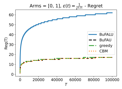
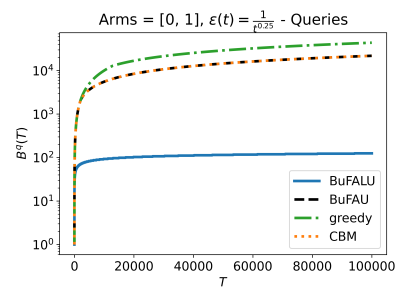
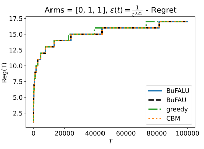
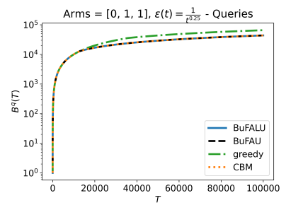
Figure 1: Performance in two deterministic instances. Left column: regret, right column: number of queries. In the top row, there is a unique optimal arm, while in the bottom one there are two. All evaluations used $\epsilon(t)=t^{-1/4}$ and tested one seed (deterministic problems).

In this section, we present a simple numerical illustration of the behavior of BuFALU in the presence of a unique or multiple optimal arms. To best capture the difference between the scenarios, we evaluate the algorithm on two deterministic MAB instances. In the first instance, the optimal arm is unique (with $\mu^{*}=1$) and there exists a single suboptimal arm (with $\mu_{1}=0$). The second instance is the same, except for an additional optimal arm. We compare BuFALU to a few natural baselines. The first uses the same querying mechanism as BuFALU but sets $c_{t}\in\operatorname*{arg\,max}_{a}UCB_{t}(a)$. This baseline, called BuFAU, will allow us to understand the contribution of the action choice vs. the querying rule. The second baseline is CBM-UCB (Efroni et al., 2021), whose problem-independent guarantees are similar to BuFALU. The final baseline is a greedy algorithm that receives a total budget as guaranteed by Theorem 2 (i.e., $\frac{6K\ln T}{\epsilon^{2}(t)}+K$). If the budget is not exhausted, it plays (and queries) the maximal UCB; otherwise, it plays (without querying) the arm with the maximal empirical mean. All algorithms are evaluated with $\epsilon(t)=t^{-1/4}$ for $100,000$ steps. Then, Theorem 2 guarantees that BuFALU cannot query any arm more than $\sim 20,000$ times. We refer to Section C.1 for a full description of the baselines and remark that evaluations in stochastic 5-armed problems yield similar insights (see Section C.2). The results are depicted in Figure 1.

The simulated behavior of BuFALU validates the characterization of Theorem 2: when there are multiple optimal arms, BuFALU uses all available budget to query them and achieves the same regret and querying performance as the baselines. In contrast, when the optimal arm is unique, BuFALU only sparingly asks for feedback – only $\sim 1/150$ fraction of the cumulative number of queries of other baselines. Its regret, however, is larger by a factor of $4$, the same factor that we get by replacing $\bar{N}(T,\Delta_{a})$ with $\bar{N}(T,\Delta_{a}/2)$. Notably, if queries have a cost $c$, the query reduction is clearly worth this degradation. In fact, for any per-query cost of $c>0.0025$ (namely, $0.25\%$ of the optimal rewards), BuFALU outperforms all baselines. Lastly, comparing BuFALU to BuFAU, we conclude that the key part in BuFALU is the choice of $c_{t}$, which allows separating a unique optimal arm from all other arms.

6 Summary and Future Work

In this work, we analyzed MAB problems where rewards must be queried to be observed. We proved lower bounds in this setting and highlighted the fundamental difference between problems with a unique and multiple optimal arms. We also presented BuFALU, to which we proved problem-dependent regret and querying bounds and showed its adaptivity to the number of optimal arms.

In the standard MAB setting, there are a few interesting directions for improving our results. First, although our analysis supports arbitrary sequences of $\epsilon(t)$, the maximization in $\bar{N}$ might be loose when $\epsilon(t)$ briefly drops. We believe that better characterizing these cases is imperative when working with general (possibly decreasing) budgets. Second, when the optimal arm is unique, our regret bounds degrade by a constant factor of $4$. Yet, the lower bounds hint that this factor does not have to affect all arms (and might, for example, be present mainly in the queries of the optimal arm). Improving this factor might require changes to the algorithm and/or confidence intervals and is left for future work. Finally, while we limited the number of queries from played arms, Yun et al. 2018 allowed budget-limited observations from unplayed arms. Although combining the settings is natural, the individual solutions are very different, and we leave this for future work.

Moreover, we only tackled the standard MAB setting. Extending our work to other settings might lead to nontrivial challenges. In large or continuous problem, e.g., combinatorial bandits, (Chen et al., 2016a), linear bandits (Abbasi-Yadkori et al., 2011) and reinforcement learning (RL, Jaksch et al., 2010; Azar et al., 2013; Simchowitz and Jamieson, 2019), the dichotomy to unique and multiple optimal arms might be too coarse. Then, it might be more relevant to characterize the behavior using the size or structure of the set of optimal actions. Specifically in RL, recent studies show that the presence of multiple optimal arms greatly affects the problem-dependent regret even without querying constraints (Xu et al., 2021; Tirinzoni et al., 2021), and it is worthwhile to further study it when feedback is limited. Alternatively, one could extend our setting to nonstationary environments, where feedback is required to track environmental changes, and to settings with some adversity in the rewards (e.g., adversarial corruptions Lykouris et al. (2018)).

Finally, our work raises important questions in the low-budget regime (e.g., logarithmic budget). There, minimizing the regret seems hopeless in the presence of multiple optimal arms, and weaker optimality notions can be considered. One option is lenient regret criteria (Merlis and Mannor, 2020), which do not incur regret when playing near-optimal arms. Then, it might be possible to perform well even when $\epsilon(t)$ does not decrease to zero, but this warrants further study.

Appendix A Lower bounds

We start by stating a variant of the fundamental inequality of [Garivier et al., 2019], proved by Efroni et al. [2021] for the case where feedback is not always observed.

Lemma 4.

For any $T\geq 1$, any $\sigma(I_{T})$-measurable random variable $Z$ with values in $[0,1]$ and any two bandit instances ${\underline{\nu}}$ and ${\underline{\nu}}^{\prime}$, it holds that

$$\sum_{a=1}^{K}\mathbb{E}_{\underline{\nu}}\left[n^{q}_{T}\left(a\right)\right]\mathrm{KL}(\nu_{a},\nu^{\prime}_{a})\geq\mathrm{kl}\left(\mathbb{E}_{\underline{\nu}}\left[Z\right],\mathbb{E}_{{\underline{\nu}}^{\prime}}\left[Z\right]\right)$$ (3)

As was shown in [Garivier et al., 2019], a similar inequality allows elegantly deriving lower bounds under various regularity assumptions on the bandit strategy.

A.1 Proof of Theorem 1

See 1

Proof.

Parts of the proof rely on techniques from Theorem 1 in [Garivier et al., 2019]. First notice that for any $p,q\in\left[0,1\right]$, it holds that

$$\mathrm{kl}(p,q) =\underbrace{p\ln\frac{1}{q}}_{\geq 0}+\underbrace{(1-p)\ln\frac{1}{1-q}}_{\geq 0}+\underbrace{p\ln p+(1-p)\ln(1-p)}_{\geq-\ln 2}$$

$$\geq\max\left\{p\ln\frac{1}{q},(1-p)\ln\frac{1}{1-q}\right\}-\ln 2$$ (4)

Proof of Part 1.

Let $a\notin\mathcal{A}_{*}({\underline{\nu}})$ be some suboptimal arm. Furthermore, let ${\underline{\nu}}^{\prime}$ be a modified bandit instance such that $\nu^{\prime}_{k}=\nu_{k}$ for all $k\neq a$ and $\nu^{\prime}_{a}\in\mathcal{D}$ is some distribution with $\mathbb{E}[\nu^{\prime}_{a}]>\mu^{*}$ (if such a distribution does not exist, then $\mathcal{K}_{\mathrm{inf}}^{+}(\nu_{a},\mu^{*},\mathcal{D})=\infty$ and the bound trivially holds). Then, by Lemma 4 with $Z=\frac{n_{T}\left(a\right)}{T}\in\left[0,1\right]$ and Equation 4, it holds that

$$\mathbb{E}_{\underline{\nu}}\left[n^{q}_{T}\left(a\right)\right]\mathrm{KL}(\nu_{a},\nu^{\prime}_{a}) \geq\mathrm{kl}\left(\frac{\mathbb{E}_{{\underline{\nu}}}\left[n_{T}\left(a\right)\right]}{T},\frac{\mathbb{E}_{{\underline{\nu}}^{\prime}}\left[n_{T}\left(a\right)\right]}{T}\right)$$

$$\geq\left(1-\frac{\mathbb{E}_{{\underline{\nu}}}\left[n_{T}\left(a\right)\right]}{T}\right)\ln\frac{1}{1-\frac{\mathbb{E}_{{\underline{\nu}}^{\prime}}\left[n_{T}\left(a\right)\right]}{T}}-\ln 2\enspace.$$ (5)

Since the bandit strategy is consistent and $a$ is suboptimal for instance ${\underline{\nu}}$, it holds that $\lim_{T\to\infty}\frac{\mathbb{E}_{{\underline{\nu}}}\left[n_{T}\left(a\right)\right]}{T}=0$. Moreover, $a$ is the unique optimal arm of bandit instance ${\underline{\nu}}^{\prime}$. Therefore, the consistency implies that for any $\alpha\in(0,1]$ and for sufficiently large $T$,

$$1-\frac{\mathbb{E}_{{\underline{\nu}}^{\prime}}\left[n_{T}\left(a\right)\right]}{T}=\frac{T-\mathbb{E}_{{\underline{\nu}}^{\prime}}\left[n_{T}\left(a\right)\right]}{T}=\frac{\sum_{a^{\prime}\neq a}\mathbb{E}_{{\underline{\nu}}^{\prime}}\left[n_{T}\left(a^{\prime}\right)\right]}{T}\leq\frac{T^{\alpha}}{T}=T^{\alpha-1}\enspace.$$

Combining both into section A.1, we get that for any $\alpha\in(0,1]$ and any $\nu^{\prime}_{a}$ with $\mathbb{E}[\nu^{\prime}_{a}]>\mu^{*}$,

$$\liminf_{T\to\infty}\frac{\mathbb{E}_{\underline{\nu}}\left[n^{q}_{T}\left(a\right)\right]}{\ln T} \geq\frac{1}{\mathrm{KL}(\nu_{a},\nu^{\prime}_{a})}\liminf_{T\to\infty}\frac{1}{\ln T}\left(\left(1-\frac{\mathbb{E}_{{\underline{\nu}}}\left[n_{T}\left(a\right)\right]}{T}\right)\ln\frac{1}{1-\frac{\mathbb{E}_{{\underline{\nu}}^{\prime}}\left[n_{T}\left(a\right)\right]}{T}}-\ln 2\right)$$

$$\geq\frac{1}{\mathrm{KL}(\nu_{a},\nu^{\prime}_{a})}\liminf_{T\to\infty}\frac{1}{\ln T}\ln\frac{1}{T^{\alpha-1}}$$

$$=\frac{1-\alpha}{\mathrm{KL}(\nu_{a},\nu^{\prime}_{a})}\enspace,$$

and since it holds for any $\alpha\in(0,1]$, we have that

$$\liminf_{T\to\infty}\frac{\mathbb{E}_{\underline{\nu}}\left[n^{q}_{T}\left(a\right)\right]}{\ln T}\geq\frac{1}{\mathrm{KL}(\nu_{a},\nu^{\prime}_{a})}\enspace.$$

By taking the supremum in the right-hand side over all distributions $\nu^{\prime}_{a}\in\mathcal{D}$ with $\mathbb{E}[\nu^{\prime}_{a}]>\mu^{*}$, we conclude this part of the proof.

Proof of Part 2.

Let $\mu\in\left[\mu^{s},\mu^{*}\right]$ and assume that there exist two distributions $\nu^{\prime}_{a},\nu^{\prime}_{a^{*}}\in\mathcal{D}$ such that $\mathbb{E}[\nu^{\prime}_{a}]\geq\mu$ and $\mathbb{E}[\nu^{\prime}_{a^{*}}]<\mu$ (otherwise, either $\mathcal{K}_{\mathrm{inf}}^{+}(\nu_{a},\mu,\mathcal{D})=\infty$ or $\mathcal{K}_{\mathrm{inf}}^{-}(\nu_{a^{*}},\mu,\mathcal{D})=\infty$ and the bound trivially holds). Also, define a new bandit instance ${\underline{\nu}}^{\prime}$ for which $\nu^{\prime}_{k}=\nu_{k}$ for all $k\neq a,a^{*}$ and arms $a,a^{*}$ are distributed according to $\nu^{\prime}_{a}$ and $\nu^{\prime}_{a^{*}}$, respectively. By Lemma 4 with $Z=\frac{n_{T}\left(a^{*}\right)}{T}\in\left[0,1\right]$ and Equation 4, it holds that

$$\mathbb{E}_{\underline{\nu}}\left[n^{q}_{T}\left(a\right)\right]\mathrm{KL}(\nu_{a},\nu^{\prime}_{a})+\mathbb{E}_{\underline{\nu}}\left[n^{q}_{T}\left(a^{*}\right)\right]\mathrm{KL}(\nu_{a^{*}},\nu^{\prime}_{a^{*}}) \geq\mathrm{kl}\left(\frac{\mathbb{E}_{{\underline{\nu}}}\left[n_{T}\left(a^{*}\right)\right]}{T},\frac{\mathbb{E}_{{\underline{\nu}}^{\prime}}\left[n_{T}\left(a^{*}\right)\right]}{T}\right)$$

$$\geq\frac{\mathbb{E}_{{\underline{\nu}}}\left[n_{T}\left(a^{*}\right)\right]}{T}\ln\frac{1}{\frac{\mathbb{E}_{{\underline{\nu}}^{\prime}}\left[n_{T}\left(a^{*}\right)\right]}{T}}-\ln 2\enspace.$$ (6)

Since the bandit strategy is consistent and $a^{*}$ is the unique optimal arm for instance ${\underline{\nu}}$, for any $a^{\prime}\neq a^{*}$ we have that $\mathbb{E}_{{\underline{\nu}}}\left[n_{T}\left(a^{\prime}\right)\right]/T\to 0$ and thus

$$\lim_{T\to\infty}\frac{\mathbb{E}_{{\underline{\nu}}}\left[n_{T}\left(a^{*}\right)\right]}{T}=\lim_{T\to\infty}\frac{T-\sum_{a^{\prime}\neq a^{*}}\mathbb{E}_{{\underline{\nu}}}\left[n_{T}\left(a^{\prime}\right)\right]}{T}=1-\sum_{a^{\prime}\neq a^{*}}\lim_{T\to\infty}\frac{\mathbb{E}_{{\underline{\nu}}}\left[n_{T}\left(a^{\prime}\right)\right]}{T}=1\enspace.$$

Moreover, $a^{*}$ is strictly suboptimal in bandit instance ${\underline{\nu}}^{\prime}$. Therefore, the consistency implies that for any $\alpha\in(0,1]$ and for sufficiently large $T$,

$$\frac{\mathbb{E}_{{\underline{\nu}}^{\prime}}\left[n_{T}\left(a^{*}\right)\right]}{T}\leq\frac{T^{\alpha}}{T}=T^{\alpha-1}\enspace.$$

Therefore, for any $\alpha\in(0,1]$, we can bound

$$\liminf_{T\to\infty}\frac{1}{\ln T}\left(\frac{\mathbb{E}_{{\underline{\nu}}}\left[n_{T}\left(a^{*}\right)\right]}{T}\ln\frac{1}{\frac{\mathbb{E}_{{\underline{\nu}}^{\prime}}\left[n_{T}\left(a^{*}\right)\right]}{T}}-\ln 2\right)\geq\liminf_{T\to\infty}\frac{1}{\ln T}\ln\frac{1}{T^{\alpha-1}}=1-\alpha\enspace,$$ (7)

and since it holds for any $\alpha\in(0,1]$, the same result holds for $\alpha=0$.

For the l.h.s., we divide into two cases:

Case I: Letting $a\in\operatorname*{arg\,max}_{a^{\prime}\neq a^{*}}\mu_{a^{\prime}}$ be an arm such that $\mu_{a}=\mu^{s}$ while choosing $\mu=\mu^{s}$ and $\nu^{\prime}_{a}=\nu_{a}$, we get that $\mathrm{KL}(\nu_{a},\nu^{\prime}_{a})=0$. Furthermore, since $a$ is strictly suboptimal and $\mathbb{E}[\nu^{\prime}_{a^{*}}]<\mu^{s}<\mu^{*}$, we have that $\mathrm{KL}(\nu_{a^{*}},\nu^{\prime}_{a^{*}})>0$. Dividing by it in (A.1) and combining with (7), we get that

$$\liminf_{T\to\infty}\frac{\mathbb{E}_{\underline{\nu}}\left[n^{q}_{T}\left(a^{*}\right)\right]}{\ln T}\geq\frac{1}{\mathrm{KL}(\nu_{a^{*}},\nu^{\prime}_{a^{*}})}\enspace.$$

By taking the supremum in the right-hand side over all distributions $\nu^{\prime}_{a^{*}}\in\mathcal{D}$ with $\mathbb{E}[\nu^{\prime}_{a^{*}}]<\mu^{s}$, we get the first desired result.

Case II: For any $\mu\in\left[\mu^{s},\mu^{*}\right]$, we apply Hölder’s inequality and bound the l.h.s. of Section A.1 by

$$\mathbb{E}_{\underline{\nu}}\left[n^{q}_{T}\left(a\right)\right]\mathrm{KL}(\nu_{a},\nu^{\prime}_{a}) +\mathbb{E}_{\underline{\nu}}\left[n^{q}_{T}\left(a^{*}\right)\right]\mathrm{KL}(\nu_{a^{*}},\nu^{\prime}_{a^{*}})$$

$$\leq\left(\mathbb{E}_{\underline{\nu}}\left[n^{q}_{T}\left(a\right)\right]+\mathbb{E}_{\underline{\nu}}\left[n^{q}_{T}\left(a^{*}\right)\right]\right)\max\left\{\mathrm{KL}(\nu_{a},\nu^{\prime}_{a}),\mathrm{KL}(\nu_{a^{*}},\nu^{\prime}_{a^{*}})\right\}\enspace.$$

Importantly, notice that $\mathrm{KL}(\nu_{a^{*}},\nu^{\prime}_{a^{*}})>0$ (since $\mathbb{E}\left[\nu^{\prime}_{a^{*}}\right]<\mu\leq\mu^{*}$) and we can divide by the maximum. Combining with (7), we get

$$\liminf_{T\to\infty}\frac{\mathbb{E}_{\underline{\nu}}\left[n^{q}_{T}\left(a\right)\right]+\mathbb{E}_{\underline{\nu}}\left[n^{q}_{T}\left(a^{*}\right)\right]}{\ln T} \geq\frac{1}{\max\left\{\mathrm{KL}(\nu_{a},\nu^{\prime}_{a}),\mathrm{KL}(\nu_{a^{*}},\nu^{\prime}_{a^{*}})\right\}}\enspace.$$

Taking the supremum over all distributions $\nu^{\prime}_{a},\nu^{\prime}_{a^{*}}\in\mathcal{D}$ with expectations $\mathbb{E}\left[\nu^{\prime}_{a}\right]>\mu$ and $\mathbb{E}\left[\nu^{\prime}_{a^{*}}\right]<\mu$ leads to the second stated result and concludes this part of the proof.

We remark that a more general lower bound can be written without applying Hölder’s inequality:

$$\mathcal{K}_{\mathrm{inf}}^{+}(\nu_{a},\mu,\mathcal{D})n^{q}_{\infty}\left(a\right)+\mathcal{K}_{\mathrm{inf}}^{-}(\nu_{a^{*}},\mu,\mathcal{D})n^{q}_{\infty}\left(a^{*}\right)\geq 1\enspace$$ (8)

for any $\mu\in\left[\mu^{s},\mu^{*}\right]$, where we define $0\cdot(+\infty)\geq 1$. Notably, this definition makes sure that the bound holds whenever any of the quantities at its l.h.s. are infinite, so it is only needed to be proven when all quantities are finite. Then, starting from (A.1), dividing by $\ln T$, taking $\liminf$ and using (7), we get that

$$\mathrm{KL}(\nu_{a},\nu^{\prime}_{a})n^{q}_{\infty}\left(a\right)+\mathrm{KL}(\nu_{a^{*}},\nu^{\prime}_{a^{*}})n^{q}_{\infty}\left(a^{*}\right)\geq 1\enspace.$$

Next, if both $\mathcal{K}_{\mathrm{inf}}^{+}(\nu_{a},\mu,\mathcal{D}),\mathcal{K}_{\mathrm{inf}}^{-}(\nu_{a^{*}},\mu,\mathcal{D})<+\infty$, we can take the infimum at the l.h.s. knowing that it is not over an empty set. Moreover, for $n^{q}_{\infty}\left(a\right),n^{q}_{\infty}\left(a^{*}\right)<+\infty$, the inequality is preserved after the infimum, which leads to Equation 8.

Proof of Part 3.

Assume that condition (1) holds. For any $a\in\mathcal{A}_{*}({\underline{\nu}})$, define a bandit instance ${\underline{\nu}}^{\prime}$ such that $\nu^{\prime}_{k}=\nu_{k}$ for all $k\neq a$ and $\nu^{\prime}_{a}\in\mathcal{D}$ is some distribution such that $\mathbb{E}\left[\nu^{\prime}_{a}\right]<\mu^{*}$ (such a distribution must exist, as otherwise, $\mathcal{K}_{\mathrm{inf}}^{-}(\nu_{a},\mu^{*},\mathcal{D})=\infty$ and condition (1) does not hold). Then, by Lemma 4 with $Z=\frac{n_{T}\left(a\right)}{T}\in\left[0,1\right]$ and Equation 4, it holds that

$$\mathbb{E}_{\underline{\nu}}\left[n^{q}_{T}\left(a\right)\right]\mathrm{KL}(\nu_{a},\nu^{\prime}_{a})\geq\mathrm{kl}\left(\frac{\mathbb{E}_{{\underline{\nu}}}\left[n_{T}\left(a\right)\right]}{T},\frac{\mathbb{E}_{{\underline{\nu}}^{\prime}}\left[n_{T}\left(a\right)\right]}{T}\right)\geq\frac{\mathbb{E}_{{\underline{\nu}}}\left[n_{T}\left(a\right)\right]}{T}\ln\frac{1}{\frac{\mathbb{E}_{{\underline{\nu}}^{\prime}}\left[n_{T}\left(a\right)\right]}{T}}-\ln 2\enspace.$$

As $a$ is strictly suboptimal in bandit instance ${\underline{\nu}}^{\prime}$, and since the bandit strategy is consistent, for any $\alpha\in(0,1]$ and for sufficiently large $T$, it holds that

$$\frac{\mathbb{E}_{{\underline{\nu}}^{\prime}}\left[n_{T}\left(a\right)\right]}{T}\leq\frac{T^{\alpha}}{T}=T^{\alpha-1}\enspace.$$

Then, for large enough $T$, we have that

$$\mathbb{E}_{\underline{\nu}}\left[n^{q}_{T}\left(a\right)\right]\mathrm{KL}(\nu_{a},\nu^{\prime}_{a})\geq\frac{\mathbb{E}_{{\underline{\nu}}}\left[n_{T}\left(a\right)\right]}{T}\ln\frac{1}{T^{\alpha-1}}-\ln 2=(1-\alpha)\frac{\mathbb{E}_{{\underline{\nu}}}\left[n_{T}\left(a\right)\right]}{T}\ln T-\ln 2\enspace.$$

Since the number of arms is finite, for large enough $T$, the inequality holds for all $a\in\mathcal{A}_{*}({\underline{\nu}})$. Then, summing over all inequalities yields

$$\sum_{a\in\mathcal{A}_{*}({\underline{\nu}})}\mathbb{E}_{\underline{\nu}}\left[n^{q}_{T}\left(a\right)\right]\mathrm{KL}(\nu_{a},\nu^{\prime}_{a})\geq(1-\alpha)\frac{\sum_{a\in\mathcal{A}_{*}({\underline{\nu}})}\mathbb{E}_{{\underline{\nu}}}\left[n_{T}\left(a\right)\right]}{T}\ln T-K\ln 2\enspace.$$ (9)

To further analyze the r.h.s. of the inequality, recall that the bandit strategy is consistent; therefore, the set of the optimal arm is sampled linearly, i.e.,

$$\lim_{T\to\infty}\frac{\sum_{a\in\mathcal{A}_{*}({\underline{\nu}})}\mathbb{E}_{{\underline{\nu}}}\left[n_{T}\left(a\right)\right]}{T} =\lim_{T\to\infty}\frac{T-\sum_{a^{\prime}\notin\mathcal{A}_{*}({\underline{\nu}})}\mathbb{E}_{{\underline{\nu}}}\left[n_{T}\left(a^{\prime}\right)\right]}{T}=1-\sum_{a^{\prime}\notin\mathcal{A}_{*}({\underline{\nu}})}\lim_{T\to\infty}\frac{\mathbb{E}_{{\underline{\nu}}}\left[n_{T}\left(a^{\prime}\right)\right]}{T}=1\,,$$

where the last equality is by the consistency, which implies that $\mathbb{E}_{{\underline{\nu}}}\left[n_{T}\left(a^{\prime}\right)\right]/T\to 0$ for any $a\notin\mathcal{A}_{*}({\underline{\nu}})$. For the l.h.s., we apply Hölder’s inequality and get

$$\sum_{a\in\mathcal{A}_{*}({\underline{\nu}})}\mathbb{E}_{\underline{\nu}}\left[n^{q}_{T}\left(a\right)\right]\mathrm{KL}(\nu_{a},\nu^{\prime}_{a})\leq\max_{a\in\mathcal{A}_{*}({\underline{\nu}})}\mathrm{KL}(\nu_{a},\nu^{\prime}_{a})\sum_{a\in\mathcal{A}_{*}({\underline{\nu}})}\mathbb{E}_{\underline{\nu}}\left[n^{q}_{T}\left(a\right)\right]\enspace.$$

Substituting both into Equation 9, reorganizing and taking the limit, we get

$$\liminf_{T\to\infty}\frac{\sum_{a\in\mathcal{A}_{*}}\mathbb{E}_{{\underline{\nu}}}\left[n^{q}_{T}\left(a\right)\right]}{\ln T}\geq(1-\alpha)\frac{1}{\max_{a\in\mathcal{A}_{*}({\underline{\nu}})}\mathrm{KL}(\nu_{a},\nu^{\prime}_{a})}\enspace.$$

Taking the supremum over all distributions $\left\{\nu^{\prime}_{a}\right\}_{a\in\mathcal{A}_{*}({\underline{\nu}})}$ in $\mathcal{D}$ such that $\mathbb{E}\left[\nu^{\prime}_{a}\right]<\mu^{*}$ and noting that the bound holds for any $\alpha\in(0,1]$ leads to the following bound:

$$\liminf_{T\to\infty}\frac{\sum_{a\in\mathcal{A}_{*}}\mathbb{E}_{{\underline{\nu}}}\left[n^{q}_{T}\left(a\right)\right]}{\ln T}\geq\frac{1}{\max_{a\in\mathcal{A}_{*}}\mathcal{K}_{\mathrm{inf}}^{-}(\nu_{a},\mu^{*},\mathcal{D})}\enspace,$$

Importantly, this bound implies that if $\mathcal{K}_{\mathrm{inf}}^{-}(\nu_{a},\mu^{*},\mathcal{D})=0$ for all $a\in\mathcal{A}_{*}({\underline{\nu}})$, then the r.h.s. is infinite and there exists at least on optimal arm $a\in\mathcal{A}_{*}({\underline{\nu}})$ for which $n^{q}_{\infty}\left(a\right)=\liminf_{T\to\infty}\frac{\mathbb{E}_{{\underline{\nu}}}\left[n^{q}_{T}\left(a\right)\right]}{\ln T}=\infty$. Moreover, one can easily verify that the derivation did not actually require condition (1); therefore, this might serve as a lower bound when the condition does not hold. Finally, as in (8), if we define $0\cdot(+\infty)\geq 1$, then using the exact same arguments, a more general version of the bound would be

$$\sum_{a\in\mathcal{A}_{*}({\underline{\nu}})}\mathcal{K}_{\mathrm{inf}}^{-}(\nu_{a},\mu^{*},\mathcal{D})n^{q}_{\infty}\left(a\right)\geq 1\enspace.$$ (10)

Assume that condition (2) holds. For any $a\in\mathcal{A}_{*}({\underline{\nu}})$, define a bandit instance ${\underline{\nu}}^{\prime}$ such that $\nu^{\prime}_{k}=\nu_{k}$ for all $k\neq a$ and $\nu^{\prime}_{a}\in\mathcal{D}$ is some distribution such that $\mathbb{E}\left[\nu^{\prime}_{a}\right]>\mu^{*}$ (we will later take an infiumum over all such distributions, and if such a distribution does not exists, then the value $\mathcal{K}_{\mathrm{inf}}^{+}(\nu_{a},\mu^{*},\mathcal{D})=\infty$ will lead to a trivial bound). Then, by Lemma 4 with $Z=\frac{n_{T}\left(a\right)}{T}\in\left[0,1\right]$ and Equation 4, it holds that

$$\mathbb{E}_{\underline{\nu}}\left[n^{q}_{T}\left(a\right)\right]\mathrm{KL}(\nu_{a},\nu^{\prime}_{a}) \geq\mathrm{kl}\left(\frac{\mathbb{E}_{{\underline{\nu}}}\left[n_{T}\left(a\right)\right]}{T},\frac{\mathbb{E}_{{\underline{\nu}}^{\prime}}\left[n_{T}\left(a\right)\right]}{T}\right)$$

$$\geq\left(1-\frac{\mathbb{E}_{{\underline{\nu}}}\left[n_{T}\left(a\right)\right]}{T}\right)\ln\frac{1}{1-\frac{\mathbb{E}_{{\underline{\nu}}^{\prime}}\left[n_{T}\left(a\right)\right]}{T}}-\ln 2\enspace.$$

As $a$ is the unique optimal arm for bandit instance ${\underline{\nu}}^{\prime}$, and since the bandit strategy is consistent, for any $\alpha\in(0,1]$ and for sufficiently large $T$ it holds that

$$1-\frac{\mathbb{E}_{{\underline{\nu}}^{\prime}}\left[n_{T}\left(a\right)\right]}{T}=\frac{T-\mathbb{E}_{{\underline{\nu}}^{\prime}}\left[n_{T}\left(a\right)\right]}{T}=\frac{\sum_{a^{\prime}\neq a}\mathbb{E}_{{\underline{\nu}}^{\prime}}\left[n_{T}\left(a^{\prime}\right)\right]}{T}\leq\frac{T^{\alpha}}{T}=T^{\alpha-1}\enspace.$$

Then, for large enough $T$, we have that

$$\mathbb{E}_{\underline{\nu}}\left[n^{q}_{T}\left(a\right)\right]\mathrm{KL}(\nu_{a},\nu^{\prime}_{a}) \geq\left(1-\frac{\mathbb{E}_{{\underline{\nu}}}\left[n_{T}\left(a\right)\right]}{T}\right)\ln\frac{1}{T^{\alpha-1}}-\ln 2$$

$$=(1-\alpha)\left(1-\frac{\mathbb{E}_{{\underline{\nu}}}\left[n_{T}\left(a\right)\right]}{T}\right)\ln T-\ln 2\enspace.$$

Next, let $a,b\in\mathcal{A}_{*}({\underline{\nu}})$ be two optimal arms. For large enough $T$, the inequality holds for both arms, and summing over their respective inequalities yields

$$\mathbb{E}_{\underline{\nu}}\left[n^{q}_{T}\left(a\right)\right]\mathrm{KL}(\nu_{a},\nu^{\prime}_{a}) +\mathbb{E}_{\underline{\nu}}\left[n^{q}_{T}\left(b\right)\right]\mathrm{KL}(\nu_{b},\nu^{\prime}_{b})$$

$$\geq(1-\alpha)\left(2-\frac{\mathbb{E}_{{\underline{\nu}}}\left[n_{T}\left(a\right)\right]}{T}-\frac{\mathbb{E}_{{\underline{\nu}}}\left[n_{T}\left(b\right)\right]}{T}\right)\ln T-2\ln 2\enspace.$$ (11)

To further analyze the r.h.s. of the inequality, notice that

$$2-\frac{\mathbb{E}_{{\underline{\nu}}}\left[n_{T}\left(a\right)\right]}{T}-\frac{\mathbb{E}_{{\underline{\nu}}}\left[n_{T}\left(b\right)\right]}{T}\geq 2-\frac{\sum_{a^{\prime}}\mathbb{E}_{{\underline{\nu}}}\left[n_{T}\left(a^{\prime}\right)\right]}{T}=2-\frac{T}{T}=1$$

For the l.h.s., we bound using Hölder’s inequality:

$$\mathbb{E}_{\underline{\nu}}\left[n^{q}_{T}\left(a\right)\right]\mathrm{KL}(\nu_{a},\nu^{\prime}_{a}) +\mathbb{E}_{\underline{\nu}}\left[n^{q}_{T}\left(b\right)\right]\mathrm{KL}(\nu_{b},\nu^{\prime}_{b})$$

$$\leq\max\left\{\mathrm{KL}(\nu_{a},\nu^{\prime}_{a}),\mathrm{KL}(\nu_{b},\nu^{\prime}_{b})\right\}\left(\mathbb{E}_{\underline{\nu}}\left[n^{q}_{T}\left(a\right)\right]+\mathbb{E}_{\underline{\nu}}\left[n^{q}_{T}\left(b\right)\right]\right)\enspace.$$

Substituting both into Section A.1, reorganizing and taking the limit, we get

$$\liminf_{T\to\infty}\frac{\mathbb{E}_{\underline{\nu}}\left[n^{q}_{T}\left(a\right)\right]+\mathbb{E}_{\underline{\nu}}\left[n^{q}_{T}\left(b\right)\right]}{\ln T}\geq(1-\alpha)\frac{1}{\max\left\{\mathrm{KL}(\nu_{a},\nu^{\prime}_{a}),\mathrm{KL}(\nu_{b},\nu^{\prime}_{b})\right\}}\enspace.$$

Taking the supremum over all distributions $\nu^{\prime}_{a},\nu^{\prime}_{b}\in\mathcal{D}$ such that $\mathbb{E}\left[\nu^{\prime}_{a}\right]>\mu^{*},\mathbb{E}\left[\nu^{\prime}_{b}\right]>\mu^{*}$ and noting that the bound holds for any $\alpha\in(0,1]$ leads to

$$\liminf_{T\to\infty}\frac{\mathbb{E}_{{\underline{\nu}}}\left[n^{q}_{T}\left(a\right)\right]+\mathbb{E}_{{\underline{\nu}}}\left[n^{q}_{T}\left(b\right)\right]}{\ln T}\geq\frac{1}{\max\left\{\mathcal{K}_{\mathrm{inf}}^{+}(\nu_{a},\mu^{*},\mathcal{D}),\mathcal{K}_{\mathrm{inf}}^{+}(\nu_{b},\mu^{*},\mathcal{D})\right\}}\enspace.$$

As we previously remarked, if one of the infimums is over an empty set, the r.h.s. equals zero and the bound trivially holds. Finally, as in the case of condition (1), if there exist two optimal arms $a,b\in\mathcal{A}_{*}({\underline{\nu}})$ for which $\mathcal{K}_{\mathrm{inf}}^{+}(\nu_{a},\mu^{*},\mathcal{D})=\mathcal{K}_{\mathrm{inf}}^{+}(\nu_{b},\mu^{*},\mathcal{D})=0$, then the r.h.s. of this bound equals infinity, and for at least one of these arms $a^{\prime}\in\left\{a,b\right\}$, it holds that $n^{q}_{\infty}\left(a^{\prime}\right)=\liminf_{T\to\infty}\frac{\mathbb{E}_{{\underline{\nu}}}\left[n^{q}_{T}\left(a^{\prime}\right)\right]}{\ln T}=\infty$. Furthermore, this bound can serve as a lower bound even when condition (2) does not hold. Finally, as in (8) and (10), if we define $0\cdot(+\infty)\geq 1$, a more general version of the bound would be

$$\mathcal{K}_{\mathrm{inf}}^{+}(\nu_{a},\mu^{*},\mathcal{D})n^{q}_{\infty}\left(a\right)+\mathcal{K}_{\mathrm{inf}}^{+}(\nu_{b},\mu^{*},\mathcal{D})n^{q}_{\infty}\left(b\right)\geq 1\enspace.$$ (12)

∎

A.2 Additional Intuition Behind the Lower Bound for multiple optimal arms

The following example illustrates the intuition behind the conditions for the third part of 1:

Example 4.

Let $x\in(0,1)$. Define $\mathcal{D}_{1}$ as the set of all distributions with the discrete support $\left\{0,1\right\}$ and expectations in $[0,x]$. Also, define $\mathcal{D}_{2}$ as the set of all distributions with the discrete support $\left\{x,1\right\}$. Particularly, for any $\nu\in\mathcal{D}_{1}$, $\mathbb{E}\left[\nu\right]\leq x$, and for any $\nu\in\mathcal{D}_{2}$, $\mathbb{E}\left[\nu\right]\geq x$. Finally, let $\mathcal{D}=\mathcal{D}_{1}\cup\mathcal{D}_{2}$. Now let ${\underline{\nu}}$ be a bandit instance with arm distributions in $\mathcal{D}$ such that $\mu^{*}=x$, i.e., the optimal reward is $x$. Then, the distribution of optimal arms is either $Ber(x)$ (if $\nu_{a^{*}}\in\mathcal{D}_{1}$) or outputs $x$ w.p. 1 (if $\nu_{a^{*}}\in\mathcal{D}_{2}$), and suboptimal arms are in $\mathcal{D}_{1}$. Consider the following instances:

1. All optimal arms are in $\mathcal{D}_{1}$. Recall that $\Omega\left(\frac{\ln{1}/{\delta}}{\epsilon^{2}}\right)$ samples are required to distinguish between $Ber(x)$ and $Ber(x-\epsilon)$ w.p. $1-\delta$. Then, any fixed logarithmic budget cannot identify whether an arm is optimal or suboptimal with arbitrarily close mean $x-\epsilon$, and at least one optimal arm must be queried super-logarithmically identify with high certainty that $\mu^{*}=x$. Notice that in this case, $\mathcal{K}_{\mathrm{inf}}^{-}(\nu_{a},x,\mathcal{D})=0$ for all optimal arms.

2. One optimal arm belongs to $\mathcal{D}_{2}$ and all other optimal arms are in $\mathcal{D}_{1}$. In this case, an agent can identify the optimal arm in $\mathcal{D}_{2}$ by a single sample, since it outputs $x$ w.p. 1 and this value is not supported by any distribution in $\mathcal{D}_{1}$. Similarly, an optimal arm can be related to $\mathcal{D}_{1}$ when outputs $0$, which only requires $\mathcal{O}\left(\frac{\ln{1}/{\delta}}{\ln{1}/(1-x)}\right)$ samples with certainty $1-\delta$. All suboptimal arms can be similarly identified. Then, with a logarithmic number of queries, agents can identify that only one arm belongs to $\mathcal{D}_{2}$, and as $\mathbb{E}\left[\nu\right]\leq\mathbb{E}\left[\nu^{\prime}\right]$ for any $\nu\in\mathcal{D}_{1}$ and $\nu^{\prime}\in\mathcal{D}_{2}$, exploiting this arm is always optimal. Thus, logarithmic queries suffice.

3. At least two optimal arms belong to $\mathcal{D}_{2}$. In this case, agents must identify that the optimal mean $\mu^{*}$ is not higher than $x$, and as in the case where all optimal arms belong to $\mathcal{D}_{1}$, a logarithmic number of queries will not suffice, as it only allows identifying the mean of an arm with a fixed accuracy. Then, all optimal arms in $\mathcal{D}_{2}$, except for a single arm, must be sampled more than a logarithmic number of times to identify that their mean is exactly $x$. In contrast, the remaining arm in $\mathcal{D}_{2}$ can be queried once to identify that it is in $\mathcal{D}_{2}$. Afterwards, as $\mathbb{E}\left[\nu\right]\geq x$ for any $\nu\in\mathcal{D}_{2}$ and $\mu^{*}=x$, this arm can be safely exploited. This corresponds to the case where $\mathcal{K}_{\mathrm{inf}}^{+}(\nu_{a},\mu^{*},\mathcal{D})=0$ for at least two optimal arms.

While the example illustrates that the conditions in the Theorem are sufficient, we actually believe that they are also necessary. In particular, when both conditions do not hold, we believe that an action-elimination algorithm that uses KL-based confidence interval [Garivier et al., 2018] should allow logarithmically querying the optimal arms. To do so, the algorithm will have to prioritize the optimal arm that might have similar distributions with higher expectations, if exists (e.g., the optimal arm in $\mathcal{D}_{2}$ in the second part of the example). However, this is not a formal proof, which we leave for future work.

A.3 Implications of the Problem-Dependent Lower Bounds to Querying Costs

We now discuss the implications of the asymptotic lower bounds when querying rewards incur a cost $c>0$. The cost might be known (e.g., payment for labeling) or unknown (e.g., user irritation in recommender systems). In this setting, it is natural to modify the regret to be query-aware:

$$\mathrm{Reg}^{q}(T)=\underbrace{\mathbb{E}\left[\sum_{t=1}^{T}\left(\mu^{*}-\mu_{a_{t}}\right)\right]}_{\text{reward suboptimality}}+\underbrace{\mathbb{E}\left[\sum_{t=1}^{T}c\mathds{1}\left\{q_{t}=1\right\}\right]}_{\text{cost penalty}} =\sum_{a=1}^{K}\left(\Delta_{a}\mathbb{E}\left[n_{T}\left(a\right)\right]+c\mathbb{E}\left[n^{q}_{T}\left(a\right)\right]\right)$$

$$\geq\sum_{a=1}^{K}\left(\Delta_{a}+c\right)\mathbb{E}\left[n^{q}_{T}\left(a\right)\right]\enspace,$$

where the inequality is since actions must be played to be queried. Assume that the regret is sub-polynomial for any instance in $\mathcal{D}$; in particular, the strategy is consistent and 1 holds.

Now, if the optimal arm is unique, then strategies must separate the optimal arm from any suboptimal arm (by 1, part 2). However, doing so with super-logarithmic queries leads to suboptimal regret due to the querying costs. Thus, optimal strategies should query all arms logarithmically, including the optimal arm. The best balance between queries from the optimal arm and increased plays from suboptimal arms depends on the values of $c$ and the gaps. However, reward degradation is unavoidable for any $c>0$.

On the other hand, if there are multiple optimal arms and the conditions of 1 (part 3) hold, then optimal arms must be queried super-logarithmically for a strategy to be consistent. Thus, no consistent strategy can achieve logarithmic query-aware regret, and every strategy must either suffer from high querying costs or low rewards.

A.4 Proofs of Proposition 1 and Corollary 2

See 1

Proof.

We follow the proof of Theorem 2 of [Garivier et al., 2019]. Let $a\notin\mathcal{A}_{*}({\underline{\nu}})$ and let ${\underline{\nu}}^{\prime}$ be some modified problem such that $\nu^{\prime}_{k}=\nu_{k}$ for all $k\neq a$ and $\nu^{\prime}_{a}\in\mathcal{D}$ is such that $\mathbb{E}[\nu^{\prime}_{a}]>\mu^{*}$ (if no such distribution exists, then $\mathcal{K}_{\mathrm{inf}}^{+}(\nu_{a},\mu^{*},\mathcal{D})=\infty$ and the r.h.s. of the lower bound is defined as $0$, so the bound trivially holds). Furthermore, notice that the desired lower bound is always smaller than $\frac{T}{K}$; therefore, if $\mathbb{E}_{{\underline{\nu}}}\left[n_{T}\left(a\right)\right]\geq\frac{T}{K}$ then the bound holds. Thus, we can assume for the rest of the proof that $\mathbb{E}_{{\underline{\nu}}}\left[n_{T}\left(a\right)\right]<\frac{T}{K}$. Finally, since the strategy is better than uniform on $\mathcal{D}$ and $a$ is the unique optimal arm in ${\underline{\nu}}^{\prime}$, it holds that $\mathbb{E}_{{\underline{\nu}}^{\prime}}\left[n_{T}\left(a\right)\right]\geq\frac{T}{K}$. Then, by Lemma 4 with $Z=\frac{n_{T}\left(a\right)}{T}\in\left[0,1\right]$, we have that

$$\mathbb{E}_{\underline{\nu}}\left[n^{q}_{T}\left(a\right)\right]\mathrm{KL}(\nu_{a},\nu^{\prime}_{a})\geq\mathrm{kl}\left(\frac{\mathbb{E}_{{\underline{\nu}}}\left[n_{T}\left(a\right)\right]}{T},\frac{\mathbb{E}_{{\underline{\nu}}^{\prime}}\left[n_{T}\left(a\right)\right]}{T}\right)\geq\mathrm{kl}\left(\frac{\mathbb{E}_{{\underline{\nu}}}\left[n_{T}\left(a\right)\right]}{T},\frac{1}{K}\right)\enspace,$$ (13)

where the last inequality is since $\frac{\mathbb{E}_{{\underline{\nu}}}\left[n_{T}\left(a\right)\right]}{T}<\frac{1}{K}$, $\frac{\mathbb{E}_{{\underline{\nu}}^{\prime}}\left[n_{T}\left(a\right)\right]}{T}\geq\frac{1}{K}$ and for $p\leq q$, the function $\mathrm{kl}(p,q^{\prime})$ is increasing in $q^{\prime}\in\left[p,q\right]$. Next, recall that by the local refinement of Pinsker’s inequality (e.g., Lemma 6 in [Garivier et al., 2019]), for any $0\leq p<q\leq 1$, we have that

$$\mathrm{kl}(p,q)\geq\frac{1}{2q}(q-p)^{2}$$

Substituting into Equation 13, we get

$$\mathbb{E}_{\underline{\nu}}\left[n^{q}_{T}\left(a\right)\right]\mathrm{KL}(\nu_{a},\nu^{\prime}_{a})\geq\frac{K}{2}\left(\frac{1}{K}-\frac{\mathbb{E}_{{\underline{\nu}}}\left[n_{T}\left(a\right)\right]}{T}\right)^{2}\enspace,$$

which can be reorganized (using $\frac{1}{K}\geq\frac{\mathbb{E}_{{\underline{\nu}}}\left[n_{T}\left(a\right)\right]}{T}$) to

$$\mathbb{E}_{{\underline{\nu}}}\left[n_{T}\left(a\right)\right]\geq\frac{T}{K}\left(1-\sqrt{2K\mathbb{E}_{\underline{\nu}}\left[n^{q}_{T}\left(a\right)\right]\mathrm{KL}(\nu_{a},\nu^{\prime}_{a})}\right)\enspace.$$

Moreover, since $\mathbb{E}_{{\underline{\nu}}}\left[n_{T}\left(a\right)\right]\leq\frac{T}{K}$, we also have that $\mathbb{E}_{{\underline{\nu}}}\left[n^{q}_{T}\left(a\right)\right]\leq\frac{T}{K}$. This leads to a bound of

$$\mathbb{E}_{{\underline{\nu}}}\left[n_{T}\left(a\right)\right]\geq\frac{T}{K}\left(1-\sqrt{2T\cdot\mathrm{KL}(\nu_{a},\nu^{\prime}_{a})}\right)\enspace.$$

Taking the maximum between both previous bounds results with

$$\mathbb{E}_{{\underline{\nu}}}\left[n_{T}\left(a\right)\right]\geq\frac{T}{K}\left(1-\sqrt{2\min\left\{K\mathbb{E}_{{\underline{\nu}}}\left[n^{q}_{T}\left(a\right)\right],T\right\}\mathrm{KL}(\nu_{a},\nu^{\prime}_{a})}\right)\enspace,$$

and taking the supremum over all distributions $\nu^{\prime}_{a}\in\mathcal{D}$ such that $\mathbb{E}\left[\nu^{\prime}_{a}\right]>\mu^{*}$ leads to the desired result. In particular, notice that the result when $\mathcal{K}_{\mathrm{inf}}^{+}(\nu_{a},\mu^{*},\mathcal{D})<\infty$ and $\mathbb{E}_{{\underline{\nu}}}\left[n^{q}_{T}\left(a\right)\right]\leq\frac{1}{8K\mathcal{K}_{\mathrm{inf}}^{+}(\nu_{a},\mu^{*},\mathcal{D})}$ directly follows from the general bound. ∎

See 2

Proof.

For generality, we only assume that $\mathbb{E}_{{\underline{\nu}}}\left[n^{q}_{t}\left(a\right)\right]\leq B_{a}(t)$, for some positive nondecreasing function $\left\{B_{a}(t)\right\}_{t\geq 1}$. First, notice that since we defined $B_{a}^{-1}(x)=0$ when $B(1)>x$, then $B_{a}^{-1}(x)$ always exists, but might be equal to $+\infty$ if $B(t)\leq x$ for all $t\in\mathbb{N}$. On the other hand, if $B_{a}^{-1}(x)=+\infty$, then the bound trivially holds (as there is no $T$ for which the result must hold). Thus, w.l.o.g., we assume that $\sup\left\{t\in\mathbb{N}:B_{a}(t)\leq x\right\}<+\infty$, and thus $B_{a}^{-1}(x)=\max\left\{t\in\mathbb{N}:B_{a}(t)\leq x\right\}$.

Moreover, by definition, for any suboptimal arm with $\frac{1}{8K\mathcal{K}_{\mathrm{inf}}^{+}(\nu_{a},\mu^{*},\mathcal{D})}<B(1)$, it holds that $B_{a}^{-1}\left(\frac{1}{8K\mathcal{K}_{\mathrm{inf}}^{+}(\nu_{a},\mu^{*},\mathcal{D})}\right)=0$, and such arms do not affect both the time constraint nor the regret bound. Therefore, we also assume w.l.o.g. that $\frac{1}{8K\mathcal{K}_{\mathrm{inf}}^{+}(\nu_{a},\mu^{*},\mathcal{D})}\geq B(1)$ for all suboptimal arms. Particularly, since $B(1)>0$, this condition also implies that $\mathcal{K}_{\mathrm{inf}}^{+}(\nu_{a},\mu^{*},\mathcal{D})<\infty$ for all $a\notin\mathcal{A}_{*}({\underline{\nu}})$.

Denote $T_{a}=B_{a}^{-1}\left(\frac{1}{8K\mathcal{K}_{\mathrm{inf}}^{+}(\nu_{a},\mu^{*},\mathcal{D})}\right)$. Then, by definition, we have that

$$\mathbb{E}_{{\underline{\nu}}}\left[n^{q}_{T_{a}}\left(a\right)\right]\leq B_{a}(T_{a})\leq\frac{1}{8K\mathcal{K}_{\mathrm{inf}}^{+}(\nu_{a},\mu^{*},\mathcal{D})}\enspace.$$

In turn, 1, leads to the bound $\mathbb{E}_{{\underline{\nu}}}\left[n_{T_{a}}\left(a\right)\right]\geq\frac{T_{a}}{2K}$. Finally, as $\mathbb{E}_{{\underline{\nu}}}\left[n_{T}\left(a\right)\right]$ is nondecreasing in $T$, for any $T\geq\max_{a\notin\mathcal{A}_{*}({\underline{\nu}})}T_{a}$, we have that

$$\mathrm{Reg}(T) =\sum_{a\notin\mathcal{A}_{*}({\underline{\nu}})}\Delta_{a}\mathbb{E}_{{\underline{\nu}}}\left[n_{T}\left(a\right)\right]$$

$$\geq\sum_{a\notin\mathcal{A}_{*}({\underline{\nu}})}\Delta_{a}\mathbb{E}_{{\underline{\nu}}}\left[n_{T_{a}}\left(a\right)\right]$$

$$\geq\sum_{a\notin\mathcal{A}_{*}({\underline{\nu}})}\Delta_{a}\frac{T_{a}}{2K}$$

$$=\sum_{a\notin\mathcal{A}_{*}({\underline{\nu}})}\frac{\Delta_{a}}{2K}B_{a}^{-1}\left(\frac{1}{8K\mathcal{K}_{\mathrm{inf}}^{+}(\nu_{a},\mu^{*},\mathcal{D})}\right)\enspace.$$

∎

Appendix B Upper Bounds

In this part of the appendix, we prove the upper bounds of Section 5. In particular, to make the proof as general as possible, we prove the upper bounds for any confidence intervals that follow some mild regularity assumptions. First recall that we denoted the history of the bandit process by $I_{t}=\left(U_{0},a_{1},q_{1},R_{1}\cdot q_{1},U_{1},\dots,a_{t},q_{t},R_{t}\cdot q_{t},U_{t}\right)$ (see Section 4), and we further define $\mathcal{F}_{t}=\sigma(I_{t})$. Then, we define regular confidence intervals as follows:

Definition 3.

Let $T\geq 1$ and let $\left\{\left[LCB_{t}(a),UCB_{t}(a)\right]\right\}_{t\in\left[T\right],a\in\left[K\right]}$ be a sequence of confidence intervals such that $LCB_{t}(a),UCB_{t}(a)$ are predictable w.r.t. $\mathcal{F}_{t}$ for any $t\in\left[T\right]$ and $a\in\left[K\right]$. Then, the confidence intervals are called regular if there exists a sequence of events $\left\{\mathbb{G}_{t}\in\mathcal{F}_{t-1}\right\}_{t\in\left[T\right]}$ (‘good events’) such that regardless of the bandit strategy, the following hold:

1. For any $t\in\left[T\right]$ and $a\in\left[K\right]$, it holds that $CI_{t}(a)\triangleq UCB_{t}(a)-LCB_{t}(a)\geq 0$.

2. For any $t\in\left[T\right]$, if $\mathbb{G}_{t}$ holds, then $\mu_{a}\in\left[LCB_{t}(a),UCB_{t}(a)\right]$ for all $a\in\left[K\right]$.

3. The failure probabilities are bounded by $\sum_{t=1}^{T}\Pr\left\{\bar{\mathbb{G}}_{t}\right\}\leq C(T)$.

4. For any $a\in\left[K\right]$, there exists a function $N_{a}^{g}:\left[T\right]\times[0,\Delta_{a}]\mapsto[0,\infty)$ such that if $\mathbb{G}_{t}$ holds, then for any $N_{a}^{g}(t,\mu)<n^{q}_{t-1}\left(a\right)\leq t-1$, it holds that $CI_{t}(a)<\mu$. Moreover, $N_{a}^{g}(t,\mu)\leq t-1$ for all $a,t$ and $\mu$ and we define $N_{a}^{g}(t,0)=t-1$.

5. There exists a function $N^{as}:\left[T\right]\times[0,\infty)\mapsto[0,\infty)$ such that for any $a\in\left[K\right]$ and $N^{as}(t,\mu)<n^{q}_{t-1}\left(a\right)\leq t-1$, it holds that $CI_{t}(a)<\mu$. Moreover, $N_{a}^{g}(t,\mu)\leq t-1$ for all $a,t$ and $\mu$ and we define $N^{as}(t,0)=t-1$.

Finally, w.l.o.g., we assume that for any $t\geq 1$, $a\in\left[K\right]$ and $\mu\in[0,\Delta_{a}]$, it holds that $N_{a}^{g}(t,\mu)\leq N^{as}(t,\mu)$, as by definition, we can always replace $N_{a}^{g}(t,\mu)$ by $\min\left\{N_{a}^{g}(t,\mu),N^{as}(t,\mu)\right\}$. Equivalently, any bound dependence in $N_{a}^{g}(t,\mu)$ can be replaced by $\min\left\{N_{a}^{g}(t,\mu),N^{as}(t,\mu)\right\}$

Each of the conditions is a reasonable requirement from confidence intervals. The first condition requires that $\left[LCB_{t}(a),UCB_{t}(a)\right]$ will be a nonempty interval. The second condition requires it to contain the true mean under some good event, while the third makes sure that the good events hold with sufficiently high probability. The last two conditions characterize the quantities that will affect the performance when using the confidence intervals: condition four quantifies the number of samples $N_{a}^{g}(t,\mu)$ required for an arm $a$ to be well-concentrated (up to a confidence level $\mu$) at time $t$ when the good event holds. Importantly, it will determine in-expectation regret and querying bounds. We emphasize that $N_{a}^{g}$ might depend on the specific arm distribution $\nu_{a}$ (e.g., be variance-dependent), but cannot depend on any random quantity. The last condition quantifies the number of samples $N^{as}(t,\mu)$ required for the confidence intervals to be smaller than $\mu$ at time $t$ regardless of the good event. In particular, this condition must hold for all arms and will determine the almost-sure querying guarantees. In practice, all these requirements are extremely mild and hold for most standard confidence intervals, including Hoeffding-based confidence intervals (as in the main paper) and Bernstein-based confidence intervals. We refer the readers to Section B.3 for the regularity proofs of these confidence intervals. We now state a more general version of Theorem 2 that characterizes the performance of Algorithm 1 when used with regular confidence intervals:

Theorem 3.

Let $T\geq 1$ and let $\{\epsilon(t)\}_{t\in\left[T\right]}$ be some nonnegative sequence. Also, let $L_{\epsilon}(T,\Delta)=\sum_{t=1}^{T}\mathds{1}\left\{\epsilon(t)\geq\Delta\right\}$ be the number of times $\epsilon(t)$ exceeds a confidence-level $\Delta\geq 0$ until $T$ and define

$$\bar{N}_{a}^{g}(T,\mu)=\max_{t\in\left[T\right]}N_{a}^{g}\left(t,\max\left\{\mu,\epsilon(t)\right\}\right),\quad\bar{N}^{as}(T)=\max_{t\in\left[T\right]}N^{as}(t,\epsilon(t))\enspace.$$

Then, when applying Algorithm 1 with regular confidence intervals, the following hold:

1. For all $a\in\left[K\right]$, it holds that $n^{q}_{T}\left(a\right)\leq\bar{N}^{as}(T)+1$.

2. If there are multiple optimal arms $(\lvert\mathcal{A}_{*}\rvert>1)$, then

   $$\mathrm{Reg}(T)\leq\sum_{a\notin\mathcal{A}_{*}}\Delta_{a}\left(\bar{N}_{a}^{g}(T,\Delta_{a})+L_{\epsilon}(T,\Delta_{a})\right)+\left(K+C(T)\right)\Delta_{\max},$$

   $$\mathbb{E}\left[B^{q}(T)\right]\leq\sum_{a=1}^{K}\bar{N}_{a}^{g}(T,\Delta_{a})+\left(K+C(T)\right)\enspace.$$

3. If the optimal arm $a^{*}$ is unique, then

   $$\mathrm{Reg}(T)\leq\sum_{a\notin\mathcal{A}_{*}}\Delta_{a}\left(\bar{N}_{a}^{g}\left(T,\frac{\Delta_{a}}{2}\right)+L_{\epsilon}(T,\Delta_{a})\right)+\left(K+C(T)\right)\Delta_{\max},$$

   $$\mathbb{E}\left[B^{q}(T)\right]\leq\sum_{a\neq a^{*}}\bar{N}_{a}^{g}\left(T,\frac{\Delta_{a}}{2}\right)+\bar{N}_{a^{*}}^{g}\left(T,\frac{\Delta_{\min}}{2}\right)+\left(K+C(T)\right)\enspace.$$

Notably, the bounds hold for any sequence of nonnegative confidence levels $\left\{\epsilon(t)\right\}_{t\geq 1}$. This stands in sharp contrast to the results of Efroni et al. [2021], which assumed that the budget is nondecreasing, a requirement that limits the valid sequences of $\epsilon(t)$. However the cost for this generaliztion is the maximization over $t\in\left[T\right]$ in $\bar{N}_{a}^{g}(T,\mu)$ and $\bar{N}^{as}(T)$. In particular, the maximization ensures that regardless of $t$, these quantities upper bound the number of samples required for the confidence intervals to be small. Nonetheless, for reasonable choices of $\epsilon(t)$, $\bar{N}_{a}^{g}(T,\mu)$ and $\bar{N}^{as}(T)$ can be easily calculated. We refer the readers to Lemma 7 and Lemma 8, where we present natural choices of $\epsilon$ for Hoeffding and Bernstein confidence intervals, respectively, and explicitly bound $\bar{N}_{a}^{g}$ and $\bar{N}^{as}$. Specifically, one favorable choice is to require $\epsilon(t)$ to be nonincreasing. Then, bounding $L_{\epsilon}$ by $L_{\epsilon}(T,\Delta)\leq\epsilon^{-1}(\Delta)\triangleq\sup\left\{t\geq 1:\epsilon(t)\geq\Delta\right\}$ is (asymptotically) tight and much easier to understand and compute. Finally, we remark that for ease of writing, in both aforementioned lemmas, $B(t)$ is the per-arm querying budget. Then, results for total querying budget (as we immediately discuss) are simply obtained by replacing $B(t)\to B(t)/K$.

When applied with Hoeffding-based confidence intervals, the theorem reduces to the results in Theorem 2, and in particular, choosing $\epsilon(t)=\sqrt{\frac{6K\ln t}{B(t)}}$ for a nondecreasing positive budget $B(t)$ also provides budget guarantees, namely, $B^{q}(T)\leq B(T)+K$. Interestingly, a similar choice with Bernstein-based confidence intervals (explicitly, $\epsilon(t)=\sqrt{\frac{6K\ln t}{B(t)-K}}+14\frac{K\ln t}{B(t)-K}$ for $B(t)>K$) provides regret bounds that depend on the variance of arms $\left\{V_{a}\right\}_{a\in\left[K\right]}$ and expected per-arm querying bounds of $\mathcal{O}\left(4V_{a}B(t)/K\right)$. Importantly, since $V_{a}\leq\frac{1}{4}$, this improves the Hoeffding-based bounds and might be dramatically lower when the variance is low.

B.1 Proof of Theorem 3

Before proving the theorem, we start by proving a few key properties on the querying mechanism and played actions of Algorithm 1:

Lemma 5.

Let $t\in\left\{K+1,\dots,T\right\}$ and assume that Algorithm 1 is run with regular confidence intervals and $\epsilon(t)\geq 0$. Then, the following hold: (i) If $q_{t}=1$, then $CI_{t}(a_{t})>\epsilon(t)$. (ii) If the good event $\mathbb{G}_{t}$ holds and $q_{t}=0$, then $\Delta_{a_{t}}\leq\epsilon(t)$.

Proof.

Part (i). When $q_{t}=1$, recall that $a_{t}=c_{t}\in\left\{l_{t},u_{t}\right\}$. We divide into two cases. If $a_{t}=l_{t}$, then a necessary condition for querying is that

$$\epsilon(t)<UCB_{t}(c_{t})-LCB_{t}(l_{t})=UCB_{t}(l_{t})-LCB_{t}(l_{t})=CI_{t}(l_{t})\enspace,$$

as required. Otherwise, $a_{t}=u_{t}$. Then, by the definition of $l_{t}$, we have that $LCB_{t}(u_{t})\leq LCB_{t}(l_{t})$ and the querying condition implies that

$$\epsilon(t)<UCB_{t}(c_{t})-LCB_{t}(l_{t})=UCB_{t}(u_{t})-LCB_{t}(l_{t})\leq UCB_{t}(u_{t})-LCB_{t}(u_{t})=CI_{t}(u_{t}),$$

which concludes this part of the proof.

Part (ii). When $q_{t}=0$, we have that $a_{t}=l_{t}$; therefore, we need to show that $\Delta_{l_{t}}\leq\epsilon(t)$. For $q_{t}=0$ to hold, at least one of the following two options must occur:

1. First option: $UCB_{t}(u_{t})\leq LCB_{t}(l_{t})$, which implies that $UCB_{t}(a)\leq LCB_{t}(l_{t})$ for all $a\neq l_{t}$. In particular, since the good event $\mathbb{G}_{t}$ holds, we have that $LCB_{t}(l_{t})\leq\mu_{l_{t}}$ and $UCB_{t}(a)\geq\mu_{a}$ for all $a\neq l_{t}$, and thus, $\mu_{a}\leq\mu_{l_{t}}$ for all $a\neq l_{t}$. Therefore, $l_{t}$ is an optimal arm and $\Delta_{l_{t}}=0\leq\epsilon(t)$.

2. Second option: $UCB_{t}(c_{t})-LCB_{t}(l_{t})\leq\epsilon(t)$. Assume w.l.o.g. that $l_{t}$ is not an optimal arm, as otherwise $\Delta_{l_{t}}=0$ and the claim naturally holds, and let $a^{*}\neq l_{t}$ be an optimal arm. Specifically, under the good event $\mathbb{G}_{t}$, it holds that

   $$UCB_{t}(u_{t})=\max_{a\neq l_{t}}UCB_{t}(a)\geq UCB_{t}(a^{*})\geq\mu_{a^{*}}=\mu^{*}\enspace.$$

   We now divide into the cases where $c_{t}=u_{t}$ and $c_{t}=l_{t}$. If $c_{t}=u_{t}$, we use the fact that under $\mathbb{G}_{t}$, $LCB_{t}(l_{t})\leq\mu_{l_{t}}$, and we get that

   $$\Delta_{l_{t}}=\mu^{*}-\mu_{l_{t}}\leq UCB_{t}(u_{t})-LCB_{t}(l_{t})\leq\epsilon(t)\enspace,$$

   where the last inequality is by the assumption that $UCB_{t}(c_{t})-LCB_{t}(l_{t})\leq\epsilon(t)$ for $c_{t}=u_{t}$. On the other hand, if $c_{t}=l_{t}$, this assumption is equivalent to $CI_{t}(l_{t})\leq\epsilon(t)$. In turn, since $l_{t}=c_{t}\in\operatorname*{arg\,max}_{a\in\left\{u_{t},l_{t}\right\}}CI_{t}(a)$, it also implies that $CI_{t}(u_{t})\leq\epsilon(t)$. Finally, under the good event, and since $l_{t}\in\operatorname*{arg\,max}_{a}LCB_{t}(a)$, we have that

   $$\mu_{l_{t}}\geq LCB_{t}(l_{t})\geq LCB_{t}(u_{t})$$

   Then, recalling that $UCB_{t}(u_{t})\geq\mu^{*}$ and $CI_{t}(u_{t})\leq\epsilon(t)$ leads to the result since

   $$\Delta_{l_{t}}=\mu^{*}-\mu_{l_{t}}\leq UCB_{t}(u_{t})-LCB_{t}(u_{t})=CI_{t}(u_{t})\leq\epsilon(t)\enspace.$$

∎

Given this lemma, we can now prove Theorem 3:

Proof.

We remark that at the first $K$ rounds, each arm is played and queried once. Then, it can be verified that all bounds hold for $T\leq K$. Thus, throughout the proof, we assume w.l.o.g. that $T>K$.

Almost-sure querying bound: Assume in contradiction that $n^{q}_{T}\left(a\right)>\bar{N}^{as}(T)+1$ for some $a\in\left[K\right]$. Therefore, there exists a time index $t\in\left\{K+1,\dots,T\right\}$ such that action $a$ was queried ($a_{t}=a$ and $q_{t}=1$) and $n^{q}_{t-1}\left(a\right)>\bar{N}^{as}(T)\geq N^{as}(t,\epsilon(t))$, where the last inequality is by the definition of $\bar{N}^{as}$. In particular, since $n^{q}_{t-1}\left(a\right)\leq t-1$, this condition cannot hold if $N^{as}(t)=t-1$. Therefore, $N^{as}(t,\epsilon(t))<t-1$, and by the definition of $N^{as}$, we have that $CI_{t}(a)<\epsilon(t)$. This come in contradiction to the fact that $a_{t}=a$ was queried, since part (i) of Lemma 5 implies that $CI_{t}(a)=CI_{t}(a_{t})>\epsilon(t)$. This proves that $n^{q}_{T}\left(a\right)\leq\bar{N}^{as}(T)+1$ for all $a\in\left[K\right]$ and concludes the first part of the proof.

Count decomposition: To derive the expected regret and querying bounds, we start with a general decomposition that will be relevant for all the required results. Specifically, the number of plays of any arm $a$ under the good event $\mathbb{G}_{t}$ (defined in Definition 3) can be bounded as follows:

$$\sum_{t=1}^{T}\mathds{1}\left\{\mathbb{G}_{t},a_{t}=a\right\}=\sum_{t=1}^{T}\mathds{1}\left\{\mathbb{G}_{t},a_{t}=a,q_{t}=0\right\}+\sum_{t=1}^{T}\mathds{1}\left\{\mathbb{G}_{t},a_{t}=a,q_{t}=1\right\}\enspace.$$ (14)

By Lemma 5 (part (i)), the first term can be bounded by

$$\sum_{t=1}^{T}\mathds{1}\left\{\mathbb{G}_{t},a_{t}=a,q_{t}=0\right\} =\sum_{t=1}^{T}\mathds{1}\left\{\mathbb{G}_{t},l_{t}=a,q_{t}=0\right\} a_{t}=l_{t} q_{t}=0$$ ( when )

$$\leq\sum_{t=1}^{T}\mathds{1}\left\{\mathbb{G}_{t},\Delta_{a}\leq\epsilon(t)\right\}$$ (By Lemma 5)

$$\leq L_{\epsilon}(T,\Delta_{a})\enspace,$$ (15)

where the last relation is by the definition of $L_{\epsilon}$. For the second term of (14), let $\Delta\geq 0$ be some parameter that will be determined later. Then, under the good event, we bound

$$\sum_{t=1}^{T}\mathds{1}\left\{\mathbb{G}_{t},a_{t}=a,q_{t}=1\right\} =\underbrace{\sum_{t=1}^{T}\mathds{1}\left\{\mathbb{G}_{t},a_{t}=a,q_{t}=1,n^{q}_{t-1}\left(a\right)\leq\bar{N}_{a}^{g}(T,\Delta)\right\}}_{\leq\bar{N}_{a}^{g}(T,\Delta)+1}$$

$$\quad+\sum_{t=1}^{T}\underbrace{\mathds{1}\left\{\mathbb{G}_{t},a_{t}=a,q_{t}=1,n^{q}_{t-1}\left(a\right)>\bar{N}_{a}^{g}(T,\Delta)\right\}}_{(*)=0\textrm{ for an appropriate $\Delta$}}$$

$$\leq\bar{N}_{a}^{g}(T,\Delta)+1\enspace,$$ (16)

which leads to a total bound of

$$\sum_{t=1}^{T}\mathds{1}\left\{\mathbb{G}_{t},a_{t}=a\right\}\leq\bar{N}_{a}^{g}(T,\Delta)+1+L_{\epsilon}(T,\Delta_{a})\enspace.$$ (17)

Proving the bound of Equation 16. The bound on the first term holds since $n^{q}_{t}\left(a\right)$ starts from zero and increases by one every time action $a$ was played and queried. We now show that depending on the assumptions and specific arms, $\Delta$ can be chosen such that under $\mathbb{G}_{t}$, the events $(*)$ of the second term cannot occur. This is trivially true if $t\leq K$, since each arm $a$ is queried at time $t=a$ with $n^{q}_{t-1}\left(a\right)=0$ and $N_{a}^{\Delta_{a}}(a)\geq 0$. Therefore, w.l.o.g., we focus on $t>K$. Moreover, by the definition of $\bar{N}_{a}^{g}$, we have that $\bar{N}_{a}^{g}(T,\Delta)\geq N_{a}^{g}(t,\max\left\{\Delta,\epsilon(t)\right\})$. Then, it suffices to show that under $\mathbb{G}_{t}$, action $a$ cannot be queried if $n^{q}_{t-1}\left(a\right)>N_{a}^{g}(t,\max\left\{\Delta,\epsilon(t)\right\})$.

To show this, first recall that $n^{q}_{t-1}\left(a\right)\leq t-1$; thus, if $N_{a}^{g}(T,\max\left\{\Delta,\epsilon(t)\right\})=t-1$, this condition can never hold. Otherwise, $N_{a}^{g}(T,\max\left\{\Delta,\epsilon(t)\right\})<t-1$, and by the regularity of the confidence interval, when $\mathbb{G}_{t}$ holds and $n^{q}_{t-1}\left(a\right)>N_{a}^{g}(T,\max\left\{\Delta,\epsilon(t)\right\})$ we have that

$$CI_{t}(a_{t})=CI_{t}(a)<\max\left\{\Delta,\epsilon(t)\right\}\enspace.$$

Importantly, if $\max\left\{\Delta,\epsilon(t)\right\}=\epsilon(t)$, then the condition of $CI_{t}(a_{t})<\epsilon(t)$ implies that an action cannot be queried (namely, $q_{t}\neq 1$), by the first part of Lemma 5. Therefore, w.l.o.g., we assume that $\max\left\{\Delta,\epsilon(t)\right\}=\Delta$ and prove by contradiction that for the right choice of $\Delta$, $a_{t}=a$ cannot be queried (under $\mathbb{G}_{t}$) if $CI_{t}(a)<\Delta$. This will imply that all indicators in $(*)$ are equal to zero and will conclude the proof of Equation 16. To do so, divide into the cases where $a$ is optimal or suboptimal and problems with unique or multiple optimal arms. In all cases, assume in contradiction that $a$ is queried and recall that it implies that $a=a_{t}=c_{t}\in\left\{l_{t},u_{t}\right\}$.

1. $a$ is an optimal arm and $\Delta=0$.
   By the regularity of the confidence intervals, $CI_{t}(a_{t})\geq 0$. Therefore, the condition $CI_{t}(a_{t})<0=\Delta$ can never hold.

2. $a$ is strictly suboptimal, $a_{t}=a=l_{t}$ and $\Delta\leq\Delta_{a}$.
   Let $a^{*}$ be any optimal arm $a^{*}$ (which is different than $l_{t}=a$ since it is suboptimal). Then, the good event implies that $UCB_{t}(a^{*})\geq\mu^{*}$, and thus

   $$UCB_{t}(u_{t})=\max_{a^{\prime}\neq l_{t}}UCB_{t}(a^{\prime})\geq UCB_{t}(a^{*})\geq\mu^{*}\enspace.$$

   On the other hand, the good event also implies that $LCB_{t}(l_{t})\leq\mu_{l_{t}}=\mu_{a}$, and by definition of $l_{t}$, it holds that $LCB_{t}(u_{t})\leq LCB_{t}(l_{t})\leq\mu_{a}$. Combining both inequalities, we get that

   $$CI_{t}(u_{t})=UCB_{t}(u_{t})-LCB_{t}(u_{t})\geq\mu^{*}-\mu_{a}=\Delta_{a}\enspace.$$

   However, since $a_{t}=l_{t}$ was played and queried, by the definition of $c_{t}$, it must hold that $CI_{t}(l_{t})\geq CI_{t}(u_{t})\geq\Delta_{a}$, in contradiction to the fact that $CI_{t}(l_{t})=CI_{t}(a)<\Delta\leq\Delta_{a}$.

3. $a$ is strictly suboptimal, $a_{t}=a=u_{t}$ and $\Delta\leq\Delta_{a}$: multiple optimal arms.
   Since there are at least two optimal arm, there exists at least one optimal arm $a^{*}$ such that $l_{t}\neq a^{*}$. Specifically, under the good event, we have that $UCB_{t}(a^{*})\geq\mu^{*}$, and then

   $$UCB_{t}(u_{t})=\max_{a^{\prime}\neq l_{t}}UCB_{t}(a^{\prime})\geq UCB_{t}(a^{*})=\mu^{*}\enspace.$$

   Moreover, under $\mathbb{G}_{t}$, we have that $LCB_{t}(u_{t})\leq\mu_{u_{t}}$, and combining both leads to

   $$CI_{t}(u_{t})=UCB_{t}(u_{t})-LCB_{t}(u_{t})\geq\mu^{*}-\mu_{u_{t}}=\Delta_{u_{t}}\enspace,$$

   in contradiction to the fact that $u_{t}=a$ and $CI_{t}(a)<\Delta\leq\Delta_{a}$.

4. $a$ is strictly suboptimal, $a_{t}=a=u_{t}$ and $\Delta\leq\Delta_{a}/2$: unique optimal arm $a^{*}$.
   Since $a_{t}=c_{t}=u_{t}$, it holds that $CI_{t}(u_{t})<\Delta\leq\frac{\Delta_{u_{t}}}{2}$. In particular, $\mathbb{G}_{t}$ implies that

   $$UCB_{t}(u_{t})=LCB_{t}(u_{t})+CI_{t}(u_{t})\leq\mu_{u_{t}}+CI_{t}(u_{t})<\mu_{u_{t}}+\frac{\Delta_{u_{t}}}{2}=\mu^{*}-\frac{\Delta_{u_{t}}}{2}\enspace.$$

   On the other hand, under $\mathbb{G}_{t}$, it holds that $UCB_{t}(a^{*})\geq\mu^{*}>UCB_{t}(u_{t})$. Then, the scenario of $a=u_{t}$ can only happen if $l_{t}=a^{*}$ (as $u_{t}$ maximizes the UCB only on actions different than $l_{t}$), and we get that

   $$LCB_{t}(l_{t}) =UCB_{t}(l_{t})-CI_{t}(l_{t})=UCB_{t}(a^{*})-CI_{t}(l_{t})\geq\mu^{*}-CI_{t}(l_{t})\enspace.$$

   Finally, since $a_{t}=c_{t}=u_{t}$, and by the definition of $c_{t}$, it holds that $CI_{t}(l_{t})\leq CI_{t}(u_{t})<\frac{\Delta_{u_{t}}}{2}$, and we have that

   $$LCB_{t}(l_{t})>\mu^{*}-\frac{\Delta_{u_{t}}}{2}>UCB_{t}(u_{t})\enspace,$$

   in contradiction to the querying rule.

5. $a=a^{*}$ is a unique optimal arm and $\Delta\leq\Delta_{\min}/2$.
   In this case, by the good event and the requirement that $CI_{t}(a)=CI_{t}(a^{*})<\Delta$,

   $$LCB_{t}(a^{*})=UCB_{t}(a^{*})-CI_{t}(a^{*})\geq\mu^{*}-CI_{t}(a^{*})>\mu^{*}-\Delta\geq\mu^{*}-\frac{\Delta_{\min}}{2}\enspace.$$

   Specifically, $LCB_{t}(a^{*})>\mu_{a}\geq LCB_{t}(a)$ for all $a\neq a^{*}$ and thus $l_{t}=a^{*}$. Furthermore, by the uniqueness of the optimal arm, $u_{t}\in\operatorname*{arg\,max}_{a\neq a^{*}}UCB_{t}(a)$ is a strictly suboptimal arm. Therefore, under $\mathbb{G}_{t}$, we have that

   $$UCB_{t}(u_{t})=LCB_{t}(u_{t})+CI_{t}(u_{t})\leq\mu_{u_{t}}+CI_{t}(u_{t})\leq\mu^{*}-\Delta_{\min}+CI_{t}(u_{t})$$

   where the last inequality is since $u_{t}$ is a suboptimal arm (and so, $\Delta_{u_{t}}\geq\Delta_{\min}$). Finally, recall that $q_{t}=1$ only if $UCB_{t}(u_{t})>LCB_{t}(l_{t})$. However, the previous inequalities imply that this condition can only hold if $CI_{t}(u_{t})>\frac{\Delta_{\min}}{2}>CI_{t}(a^{*})=CI_{t}(l_{t})$, and then $c_{t}=\operatorname*{arg\,max}_{a\in\left\{u_{t},l_{t}\right\}}CI_{t}(a)=u_{t}$. Thus, if an arm is indeed queried, it is a strictly suboptimal arm, in contradiction to the requirement that $a=a^{*}$ is queried.

Overall, when there are multiple optimal arms, cases (i)-(iii) all hold for the choice $\Delta=\Delta_{a}$. When the optimal arm is unique, cases (ii), (iv) and (v) hold with $\Delta=\Delta_{a}/2$ for suboptimal arms and $\Delta=\Delta_{\min}/2$ for the optimal arm.

Regret and queries bounds. We now show how the bounds of (16) and (17) can be used to derive the desired regret and querying bounds. To bound the expected regret, we use Equation 17 with $\Delta=\mu_{a}$ for all suboptimal arms $a\notin\mathcal{A}_{*}$, where $\mu_{a}=\Delta_{a}$ if there are multiple optimal arms and $\mu_{a}=\Delta_{a}/2$ if the optimal arm is unique. Doing so while using the failure probabilities of the good event $\mathbb{G}_{t}$, we get:

$$\mathrm{Reg}(T)=\sum_{t=1}^{T}\mathbb{E}\left[\Delta_{a_{t}}\right] \leq\sum_{t=1}^{T}\mathbb{E}\left[\Delta_{a_{t}}\mathds{1}\left\{\mathbb{G}_{t}\right\}\right]+\Delta_{\max}\sum_{t=1}^{T}\mathbb{E}\left[\mathds{1}\left\{\bar{\mathbb{G}}_{t}\right\}\right]$$

$$=\sum_{a\notin\mathcal{A}_{*}}\Delta_{a}\mathbb{E}\left[\sum_{t=1}^{T}\mathds{1}\left\{\mathbb{G}_{t},a_{t}=a\right\}\right]+\Delta_{\max}\underbrace{\sum_{t=1}^{T}\Pr\left\{\bar{\mathbb{G}}_{t}\right\}}_{\leq C(T)}$$

$$\leq\sum_{a\notin\mathcal{A}_{*}}\Delta_{a}\left(\bar{N}_{a}^{g}(T,\mu_{a})+L_{\epsilon}(T,\Delta_{a})+1\right)+\Delta_{\max}C(T)$$

$$\leq\sum_{a\notin\mathcal{A}_{*}}\Delta_{a}\left(\bar{N}_{a}^{g}(T,\mu_{a})+L_{\epsilon}(T,\Delta_{a})\right)+\left(K+C(T)\right)\Delta_{\max}\enspace.$$

Notice that substituting $\mu_{a}$ leads to the desired bound, whether there is a unique or multiple optimal arms. We similarly use Equation 16 to bound the expected number of queries. We still choose the same values of $\mu_{a}$ for suboptimal arms, but for optimal arms, we let $\mu_{a}=0=\Delta_{a}$ for all $a\in\mathcal{A}_{*}$ when there are multiple optimal arms and $\mu_{a^{*}}=\Delta_{\min}/2$ for a unique optimal arm. Then, as in the regret bound, we get

$$\mathbb{E}\left[B^{q}(T)\right]=\sum_{t=1}^{T}\mathbb{E}\left[\mathds{1}\left\{q_{t}=1\right\}\right] \leq\sum_{t=1}^{T}\mathbb{E}\left[\mathds{1}\left\{\mathbb{G}_{t},q_{t}=1\right\}\right]+\sum_{t=1}^{T}\mathbb{E}\left[\mathds{1}\left\{\bar{\mathbb{G}}_{t}\right\}\right]$$

$$=\sum_{a\in\left[K\right]}\mathbb{E}\left[\sum_{t=1}^{T}\mathds{1}\left\{\mathbb{G}_{t},a_{t}=a,q_{t}=1\right\}\right]+\underbrace{\sum_{t=1}^{T}\Pr\left\{\bar{\mathbb{G}}_{t}\right\}}_{\leq C(T)}$$

$$\leq\sum_{a\in\left[K\right]}(\bar{N}_{a}^{g}(T,\mu_{a})+1)+C(T)$$

$$=\sum_{a\in\mathcal{A}_{*}}\bar{N}_{a}^{g}(T,\mu_{a})+\sum_{a\notin\mathcal{A}_{*}}\bar{N}_{a}^{g}(T,\mu_{a})+K+C(T)\enspace.$$

and one can easily verify that substituting $\mu_{a}$ leads to both desired bounds. ∎

Remark 1.

Notice that the bounds of (16) and (17) hold even if $\epsilon(t)$ is $\mathcal{F}_{t}$ predictable, e.g., if the sequence $\left\{\epsilon(t)\right\}_{t\geq 1}$ is chosen by an adaptive adversary. Specifically, when this is the case, all bounds remain the same, except an expectation that should be taken on $\bar{N}_{a}^{g}(T,\mu)$ and $L_{\epsilon}(T,\Delta)$. Similarly, an expectation can be taken over any stochastic source that affects $\epsilon(t)$ and is independent of $\mathcal{F}_{t}$.

B.2 Problem-Independent Upper Bound

In this section, we generalize Proposition 3 to the setting presented in Appendix B.

Proposition 6.

Under the notations of Theorem 3, let $T\geq 1$ and assume that $\epsilon(t)\geq 0$ for all $t\in\left[T\right]$ and that Algorithm 1 is applied with regular confidence intervals. Also, assume that there exist a function $M(t,\Delta_{0})$ such that for all $\Delta_{0}>0$ and all arms $a\in\left[K\right]$ with $\Delta_{a}>\Delta_{0}$, it holds that $\Delta_{a}\bar{N}_{a}^{g}(T,\Delta_{a})\leq M(T,\Delta_{0})$. Then,

$$\mathrm{Reg}(T)\leq\inf_{\Delta_{0}>0}\left\{2KM\left(T,\frac{\Delta_{0}}{2}\right)+\Delta_{0}T\right\}+\sum_{t=1}^{T}\epsilon(t)+\left(K+C(T)\right)\Delta_{\max}\enspace.$$

See that for Hoeffding-based confidence intervals, we have that $\bar{N}_{a}^{g}(T,\mu)\leq\frac{6\ln T}{\mu^{2}}$ (by Lemma 7), so for any $\Delta_{a}>\Delta_{0}$, it holds that $\Delta_{a}\bar{N}_{a}^{g}(T,\Delta_{a})=\frac{6\ln T}{\Delta_{a}}\leq\frac{6\ln T}{\Delta_{0}}\triangleq M\left(T,\Delta_{0}\right)$. Then, the infimum in the bound is achieved for $\Delta_{0}=\sqrt{\frac{24K\ln T}{T}}$, which leads to the bound in the main paper (Proposition 3). Alternatively, when using Bernstein-type confidence bounds, we can bound the variance of arms by $V_{a}\leq\frac{1}{4}$ and obtain a similar bound (by Lemma 8):

$$\Delta_{a}\bar{N}_{a}^{g}(T,\Delta_{a})\leq\frac{24V_{a}\ln T}{\Delta_{a}}+52\ln T+\Delta_{a}\leq\frac{6\ln T}{\Delta_{0}}+52\ln T+\Delta_{\max}\triangleq M\left(T,\Delta_{0}\right)\enspace.$$

On the other hand, if the variance of all suboptimal arms is upper bounded by $V_{a}\leq V$, this can be used to achieve an improved variance-dependent regret bound.

Proof.

As in the problem-dependent bound of Theorem 3, we decompose the regret by:

$$\mathrm{Reg}(T)=\sum_{t=1}^{T}\mathbb{E}\left[\Delta_{a_{t}}\right] \leq\sum_{t=1}^{T}\mathbb{E}\left[\Delta_{a_{t}}\mathds{1}\left\{\mathbb{G}_{t}\right\}\right]+\Delta_{\max}\sum_{t=1}^{T}\mathbb{E}\left[\mathds{1}\left\{\bar{\mathbb{G}}_{t}\right\}\right]$$

$$\leq\sum_{a\notin\mathcal{A}_{*}}\Delta_{a}\mathbb{E}\left[\sum_{t=1}^{T}\mathds{1}\left\{\mathbb{G}_{t},a_{t}=a\right\}\right]+\Delta_{\max}C(T)\enspace.$$

Next, for any $\Delta_{0}>0$, we can bound the regret by

$$\mathrm{Reg}(T) \leq\underbrace{\sum_{a:\Delta_{a}>\Delta_{0}}\Delta_{a}\mathbb{E}\left[\sum_{t=1}^{T}\mathds{1}\left\{\mathbb{G}_{t},a_{t}=a\right\}\right]}_{(i)}+\underbrace{\sum_{a:\Delta_{a}\in(0,\Delta_{0}]}\Delta_{a}\mathbb{E}\left[\sum_{t=1}^{T}\mathds{1}\left\{\mathbb{G}_{t},a_{t}=a\right\}\right]}_{(ii)}$$

$$\quad+\Delta_{\max}C(T)\enspace.$$ (18)

To bound term $(i)$ we further decompose it to

$$(i) =\mathbb{E}\left[\sum_{a:\Delta_{a}>\Delta_{0}}\Delta_{a}\sum_{t=1}^{T}\mathds{1}\left\{\mathbb{G}_{t},a_{t}=a,q_{t}=1\right\}\right]+\mathbb{E}\left[\sum_{a:\Delta_{a}>\Delta_{0}}\sum_{t=1}^{T}\Delta_{a}\mathds{1}\left\{\mathbb{G}_{t},a_{t}=a,q_{t}=0\right\}\right]$$

$$\leq\mathbb{E}\left[\underbrace{\sum_{a:\Delta_{a}>\Delta_{0}}\Delta_{a}\sum_{t=1}^{T}\mathds{1}\left\{\mathbb{G}_{t},a_{t}=a,q_{t}=1\right\}}_{(*)}\right]+\mathbb{E}\left[\underbrace{\sum_{t=1}^{T}\Delta_{a_{t}}\mathds{1}\left\{\mathbb{G}_{t},q_{t}=0\right\}}_{(**)}\right]$$

For term $(*)$, if there are multiple optimal arms, then by Equation 16 with $\Delta=\Delta_{a}$,

$$\sum_{a:\Delta_{a}>\Delta_{0}}\Delta_{a}\sum_{t=1}^{T}\mathds{1}\left\{\mathbb{G}_{t},a_{t}=a,q_{t}=1\right\}\leq\sum_{a:\Delta_{a}>\Delta_{0}}\Delta_{a}\left(\bar{N}_{a}^{g}(T,\Delta_{a})+1\right)\leq KM\left(T,\frac{\Delta_{0}}{2}\right)+K\Delta_{\max}\enspace,$$

where the last inequality is since the gaps of all arms in the summation are larger than $\Delta_{0}$, and specifically larger than $\Delta_{0}/2$, and by bounding the number of arms with gaps larger than $\Delta_{0}$ by $K$. Alternatively, if there is a unique optimal arm, we can bound using Equation 16 with $\Delta=\Delta_{a}/2$:

$$\sum_{a:\Delta_{a}>\Delta_{0}}\Delta_{a}\sum_{t=1}^{T}\mathds{1}\left\{\mathbb{G}_{t},a_{t}=a,q_{t}=1\right\} \leq\sum_{a:\Delta_{a}>\Delta_{0}}\Delta_{a}\left(\bar{N}_{a}^{g}\left(T,\frac{\Delta_{a}}{2}\right)+1\right)$$

$$\leq 2\sum_{a:\Delta_{a}>\Delta_{0}}\frac{\Delta_{a}}{2}\bar{N}_{a}^{g}\left(T,\frac{\Delta_{a}}{2}\right)+K\Delta_{\max}$$

$$\leq 2KM\left(T,\frac{\Delta_{0}}{2}\right)+K\Delta_{\max}\enspace,$$

where the last inequality is again by the definition of $M\left(T,\frac{\Delta_{0}}{2}\right)$. Combining both cases, we get

$$(*)\leq 2KM\left(T,\frac{\Delta_{0}}{2}\right)+K\Delta_{\max}\enspace.$$

The remaining summation $(**)$ can be bounded using the fact that if $q_{t}=0$, then $\Delta_{a_{t}}\leq\epsilon(t)$ (by Lemma 5), and thus

$$(**)=\sum_{t=1}^{T}\Delta_{a_{t}}\mathds{1}\left\{\mathbb{G}_{t},q_{t}=0\right\} \leq\sum_{t=1}^{T}\Delta_{a_{t}}\mathds{1}\left\{\Delta_{a_{t}}\leq\epsilon(t)\right\}\leq\sum_{t=1}^{T}\epsilon(t)\mathds{1}\left\{\Delta_{a_{t}}\leq\epsilon(t)\right\}\leq\sum_{t=1}^{T}\epsilon(t)\enspace,$$

which lead to the bound of

$$(i)\leq 2KM\left(T,\frac{\Delta_{0}}{2}\right)+\sum_{t=1}^{T}\epsilon(t)+K\Delta_{\max}$$

Finally, we bound term $(ii)$ as follows:

$$\sum_{a:\Delta_{a}\in(0,\Delta_{0}]}\Delta_{a}\mathbb{E}\left[\sum_{t=1}^{T}\mathds{1}\left\{\mathbb{G}_{t},a_{t}=a\right\}\right] \leq\Delta_{0}\mathbb{E}\left[\sum_{a=1}^{K}\sum_{t=1}^{T}\mathds{1}\left\{\mathbb{G}_{t},a_{t}=a\right\}\right]=\Delta_{0}\mathbb{E}\left[\sum_{t=1}^{T}\mathds{1}\left\{\mathbb{G}_{t}\right\}\right]\leq\Delta_{0}T\enspace.$$

Substituting $(i)$ and $(ii)$ into Equation 18 and taking the infimum over all possible choices of $\Delta_{0}>0$ leads to the desired bound. ∎

B.3 Regularity Proofs

B.3.1 Hoeffding-Based Confidence Intervals

Hoeffding-based confidence intervals are probably the most commonly used confidence intervals for bounded (and subgaussian) rewards. Specifically, for rewards bounded in $[0,1]$, they are defined by

$$UCB_{t}(a)=\hat{\mu}_{t-1}\left(a\right)+\sqrt{\frac{3\ln t}{2n^{q}_{t-1}\left(a\right)}}\qquad\textrm{and}\qquad LCB_{t}(a)=\hat{\mu}_{t-1}\left(a\right)-\sqrt{\frac{3\ln t}{2n^{q}_{t-1}\left(a\right)}}\enspace,$$

and if $n^{q}_{t-1}\left(a\right)=0$, we define $UCB_{t}(a)=+\infty$ and $LCB_{t}(a)=-\infty$. In the following, we prove that such confidence intervals are regular:

Lemma 7.

Assume that the rewards are bounded in $\left[0,1\right]$. Then, for any $T\geq 1$, Hoeffding-based confidence intervals are regular w.r.t. the events $\mathbb{G}_{t}=\{\forall a\in\left[K\right]:\mu_{a}\in\left[LCB_{t}(a),UCB_{t}(a)\right]\}$ and the functions

$$C(t)=2K,\qquad N_{a}^{g}(t,\mu)=N^{as}(t,\mu)=\min\left\{\frac{6\ln t}{\mu^{2}},t-1\right\}\enspace,$$

Specifically, $\bar{N}_{a}^{g}(T,0)=\bar{N}^{as}(T)$. Moreover, for any $\mu>0$, it holds that $\bar{N}_{a}^{g}(T,\mu)\leq\frac{6\ln T}{\mu^{2}}$. Finally, if $B(t)$ is a positive nondecreasing sequence and $\epsilon(t)=\sqrt{\frac{6\ln t}{B(t)}}$, or, alternatively, $\epsilon(t)$ is a nonnegative nonincreasing sequence, then $\bar{N}_{a}^{g}(T,\mu)=\min\left\{\frac{6\ln T}{\max\left\{\mu^{2},\epsilon^{2}(t)\right\}},T-1\right\}$.

Proof.

Notice that $CI_{t}(a)=\sqrt{\frac{6\ln t}{n^{q}_{t-1}\left(a\right)}}$. We now check the conditions by their order:

1. The condition that $CI_{t}(a)\geq 0$ trivially holds for any $n^{q}_{t-1}\left(a\right)\geq 1$ and holds by definition when $n^{q}_{t-1}\left(a\right)=0$ (and $CI_{t}(a)=\infty$).

2. By definition, for any $t\geq 1$, if $\mathbb{G}_{t}$ holds, then $\mu_{a}\in\left[LCB_{t}(a),UCB_{t}(a)\right]$ for all $a\in\left[K\right]$, as required.

3. We now bound $\Pr\left\{\bar{\mathbb{G}}_{t}\right\}$. For any $a\in\left[K\right]$, let $X_{a}(1),\dots X_{a}(T)$ be i.i.d. random variables of the same distribution as arm $a$, and we let the observed reward at the $n^{q}_{t}\left(a\right)^{th}$ time the arm was played be $R_{t}=X_{a}(n^{q}_{t}\left(a\right))$. Then, we can write:

   $$\Pr\left\{\bar{\mathbb{G}}_{t}\right\} =\Pr\left\{\exists a\in\left[K\right]:\mu_{a}\notin\left[LCB_{t}(a),UCB_{t}(a)\right]\right\}$$

   $$=\Pr\left\{\exists a\in\left[K\right]:\left\lvert\hat{\mu}_{t-1}\left(a\right)-\mu_{a}\right\rvert>\sqrt{\frac{3\ln t}{2n^{q}_{t-1}\left(a\right)}}\right\}$$

   $$\overset{(1)}{\leq}\sum_{a=1}^{K}\Pr\left\{\left\lvert\hat{\mu}_{t-1}\left(a\right)-\mu_{a}\right\rvert>\sqrt{\frac{3\ln t}{2n^{q}_{t-1}\left(a\right)}}\right\}$$

   $$\overset{(2)}{\leq}\sum_{a=1}^{K}\sum_{n=1}^{t-1}\Pr\left\{\left\lvert\hat{\mu}_{t-1}\left(a\right)-\mu_{a}\right\rvert>\sqrt{\frac{3\ln t}{2n^{q}_{t-1}\left(a\right)}},n^{q}_{t-1}\left(a\right)=n\right\}$$

   $$\overset{(3)}{=}\sum_{a=1}^{K}\sum_{n=1}^{t-1}\Pr\left\{\left\lvert\frac{1}{n}\sum_{k=1}^{n}X_{a}(k)-\mu_{a}\right\rvert>\sqrt{\frac{3\ln t}{2n}},n^{q}_{t-1}\left(a\right)=n\right\}$$

   $$\leq\sum_{a=1}^{K}\sum_{n=1}^{t-1}\Pr\left\{\left\lvert\frac{1}{n}\sum_{k=1}^{n}X_{a}(k)-\mu_{a}\right\rvert>\sqrt{\frac{3\ln t}{2n}}\right\}$$

   $$\overset{(4)}{\leq}\sum_{a=1}^{K}\sum_{n=1}^{t-1}\frac{1}{t^{3}}$$

   $$\leq\frac{K}{t^{2}}\enspace.$$

   Relations $(1)$ and $(2)$ are due to the union bound over actions $a\in\left[K\right]$ and $n^{q}_{t-1}\left(a\right)\in\left\{0,\dots,t-1\right\}$, respectively. Moreover, notice that the relevant event cannot occur when $n^{q}_{t-1}\left(a\right)=0$, so we only treat values larger than $1$. In $(3)$ we substituted $n^{q}_{t-1}\left(a\right)=n$ and wrote the empirical means using $X_{a}(t)$. Finally, $(4)$ relies on Hoeffding’s inequality for i.i.d. bounded random variables supported by $[0,1]$. Summing over all time indices leads to the desired result:

   $$\sum_{t=1}^{T}\Pr\left\{\bar{\mathbb{G}}_{t}\right\}\leq\sum_{t=1}^{T}\frac{K}{t^{2}}\leq\sum_{t=1}^{\infty}\frac{K}{t^{2}}\leq 2K=C(T)\enspace.$$

4. If $N_{a}^{g}(t,\mu)=t-1$, then the event that $N_{a}^{g}(t,\mu)<n^{q}_{t-1}\left(a\right)\leq t-1$ can never happen, so assume w.l.o.g. that $N_{a}^{g}(t,\mu)<t-1$ and $N_{a}^{g}(t,\mu)=\frac{6\ln t}{\mu^{2}}$. In particular, $\mu>0$ and $t>1$, and it can be easily verified that whether the good event holds or not, if $n^{q}_{t-1}\left(a\right)>N_{a}^{g}(t,\mu)=\frac{6\ln t}{\mu^{2}}$, then

   $$CI_{t}(a)=\sqrt{\frac{6\ln t}{n^{q}_{t-1}\left(a\right)}}<\sqrt{\frac{6\ln t}{N_{a}^{g}(t,\mu)}}=\mu\enspace.$$

5. The proof follows exactly as the previous part, as its result did not depend on the good event.

We now prove the claims at the end of the lemma. First, for any nonnegative sequence $\left\{\epsilon(t)\right\}_{t\geq 1}$, it holds that

$$\bar{N}_{a}^{g}(T,\mu) =\max_{t\in\left[T\right]}N_{a}^{g}(t,\max\left\{\mu,\epsilon(t)\right\})$$

$$=\max_{t\in\left[T\right]}\left\{\min\left\{\frac{6\ln t}{\max\left\{\mu^{2},\epsilon^{2}(t)\right\}},t-1\right\}\right\}$$

$$\leq\max_{t\in\left[T\right]}\left\{\min\left\{\frac{6\ln t}{\mu^{2}},t-1\right\}\right\}$$

$$\leq\min\left\{\frac{6\ln T}{\mu^{2}},T-1\right\}$$

where the last inequality is since the logarithmic and constant functions are nondecreasing in $t$, and the minimum of nondecreasing functions is nondecreasing (9). Finally, we write

$$N_{a}^{g}(t,\max\left\{\mu,\epsilon(t)\right\})=\min\left\{\frac{6\ln t}{\mu^{2}},\frac{6\ln t}{\epsilon^{2}(t)},t-1\right\}\enspace.$$

Moreover, if either $\epsilon(t)=\sqrt{\frac{6\ln t}{B(t)}}$, for nondecreasing positive $B(t)$, or $\epsilon(t)\geq 0$ is nonincreasing, then $\frac{6\ln t}{\epsilon^{2}(t)}$ is nondecreasing in $t$. Thus, $N_{a}^{g}(t,\max\left\{\mu,\epsilon(t)\right\})$ is a minimum of nondecreasing functions and is nondecreasing by itself (by 9). In turn, this implies that

$$\bar{N}_{a}^{g}(T,\mu) =\max_{t\in\left[T\right]}N_{a}^{g}(t,\max\left\{\mu,\epsilon(t)\right\})=N_{a}^{g}(T,\max\left\{\mu,\epsilon(T)\right\})$$

$$=\min\left\{\frac{6\ln T}{\max\left\{\mu^{2},\epsilon^{2}(t)\right\}},T-1\right\}\enspace.$$

∎

B.3.2 Bernstein-Based Confidence Intervals

Bernstein-based confidence intervals are confidence intervals that depend on the variance on the reward distributions. Specifically, we apply Empirical-Bernstein bounds [Maurer and Pontil, 2009], which depend on the empirical variance of arms and obviate the need to know the true variances of arms. Formally, if all arm distributions are bounded in $[0,1]$ and of variances $\left\{V_{a}\right\}_{a\in\left[K\right]}$, we denote the unbiased empirical estimator of the variance by

$$\hat{V}_{t}(a)=\frac{n^{q}_{t}\left(a\right)}{n^{q}_{t}\left(a\right)-1}\left(\frac{1}{n^{q}_{t}\left(a\right)}\sum_{s=1}^{t}R_{t}^{2}\mathds{1}\left\{a_{t}=a\right\}-\left(\hat{\mu}_{t}\left(a\right)\right)^{2}\right)\enspace,$$

where we define $\hat{V}_{t}(a)=0$ if $n^{q}_{t}\left(a\right)<2$. Then, Bernstein-based confidence intervals are defined by

$$UCB_{t}(a)=\hat{\mu}_{t-1}\left(a\right)+\sqrt{\frac{6\hat{V}_{t-1}(a)\ln t}{n^{q}_{t-1}\left(a\right)}}+\frac{7\ln t}{n^{q}_{t-1}\left(a\right)-1}\enspace,$$

$$LCB_{t}(a)=\hat{\mu}_{t-1}\left(a\right)-\sqrt{\frac{6\hat{V}_{t-1}(a)\ln t}{n^{q}_{t-1}\left(a\right)}}-\frac{7\ln t}{n^{q}_{t-1}\left(a\right)-1},$$

where if $n^{q}_{t-1}\left(a\right)\leq 1$, we define $UCB_{t}(a)=+\infty$ and $LCB_{t}(a)=-\infty$ (and in general, we let $\frac{\ln t}{n^{q}_{1}\left(a\right)}=\frac{\ln t}{n^{q}_{t}\left(a\right)-1}=+\infty$ for $n^{q}_{t}\left(a\right)\leq 1$). We now prove that these confidence intervals are regular:

Lemma 8.

Assume that the rewards are bounded in $\left[0,1\right]$ and let $T\geq 1$. Then, Bernstein-based confidence interval are regular w.r.t. the events

$$\mathbb{G}_{t}=\left\{\forall a\in\left[K\right]:\mu_{a}\in\left[LCB_{t}(a),UCB_{t}(a)\right],\;\left\lvert\sqrt{\hat{V}_{t-1}(a)}-\sqrt{V_{a}}\right\rvert\leq\sqrt{\frac{6\ln t}{n^{q}_{t-1}\left(a\right)-1}}\right\}$$

and the functions

$$C(t)=12K,\qquad N_{a}^{g}(t,\mu)=\min\left\{\frac{24V_{a}\ln t}{\mu^{2}}+\frac{52\ln t}{\mu}+1,t-1\right\}\enspace.$$

For $N^{as}(t,\mu)$, we allow two different options:

$$N_{1}^{as}(t,\mu)=\min\left\{\frac{6\ln t}{\mu^{2}}+\frac{28\ln t}{\mu}+1,t-1\right\},\qquad\textrm{or}$$

$$N_{2}^{as}(t,\mu)=\min\left\{\left(\sqrt{\frac{3\ln t}{2\mu^{2}}}+\sqrt{\frac{3\ln t}{2\mu^{2}}+\frac{14\ln t}{\mu}}\right)^{2}+1,t-1\right\}$$

Specifically, we have that $\bar{N}_{a}^{g}(T,\mu)\leq N_{a}^{g}(T,\mu)$. Finally, we suggest two choices for $\epsilon(t)$:

• For nonincreasing sequence $\epsilon(t)\geq 0$, we have that $\bar{N}_{a}^{g}(T,\mu)=N_{a}^{g}(T,\max\left\{\mu,\epsilon(T)\right\})$ and $\bar{N}_{i}^{as}(T)=N_{i}^{as}(T,\epsilon(T))$ for $i=1,2$.

• If $B(t)$ is a nondecreasing sequence such that $B(1)>1$ and $\epsilon(t)=\sqrt{\frac{6\ln t}{B(t)-1}}+14\frac{\ln t}{B(t)-1}$, we work with $N_{2}^{as}(t,\epsilon(t))=\min\left\{B(t),t-1\right\}$, and thus, $\bar{N}_{2}^{as}(T)=\min\left\{B(T),T-1\right\}$. Moreover, for this choice, we have that

  $$\bar{N}_{a}^{g}(T,\mu)\leq\min\left\{N_{a}^{g}(T,\mu),4V_{a}(B(T)-1)+\min\left\{22\sqrt{(B(T)-1)\ln T},4(B(T)-1)\right\}+1\right\}.$$

Proof.

First note that for any $a\in\left[K\right]$ and $t\geq 1$, the width of the confidence interval is

$$CI_{t}(a)=2\sqrt{\frac{6\hat{V}_{t-1}(a)\ln t}{n^{q}_{t-1}\left(a\right)}}+14\frac{\ln t}{n^{q}_{t-1}\left(a\right)-1}\enspace.$$

We now verify each of the regularity requirements:

1. The condition that $CI_{t}(a)\geq 0$ trivially holds for any $t\geq 1$ when $n^{q}_{t-1}\left(a\right)\geq 2$, as $\hat{V}_{t-1}(a)\geq 0$ and $\ln T\geq 0$, and hold by definition when $n^{q}_{t-1}\left(a\right)\leq 1$, as then, $CI_{t}(a)=+\infty$.

2. By definition, under $\mathbb{G}_{t}$, $\mu_{a}\in\left[LCB_{t}(a),UCB_{t}(a)\right]$ for any $t\geq 1$ and $a\in\left[K\right]$.

3. We now bound $\Pr\left\{\bar{\mathbb{G}}_{t}\right\}$. For any $a\in\left[K\right]$, let $X_{a}(1),\dots X_{a}(T)$ be i.i.d. random variables of the same distribution as arm $a$, and we let the observed reward at the $n^{q}_{t}\left(a\right)^{th}$ time the arm was played be $R_{t}=X_{a}(n^{q}_{t}\left(a\right))$. We also denote the unbiased empirical estimator of the variance based on the first $n$ samples by

   $$\bar{V}_{n}(a)=\frac{n}{n-1}\left(\frac{1}{n}\sum_{k=1}^{n}X_{a}^{2}(k)-\left(\frac{1}{n}\sum_{k=1}^{n}X_{a}(k)\right)^{2}\right)\enspace,$$

   which equals $\hat{V}_{t-1}(a)$ when $n^{q}_{t-1}\left(a\right)=n$. Then, we can write:

   $$\Pr\left\{\bar{\mathbb{G}}_{t}\right\} =\Pr\Biggl{\{}\exists a\in\left[K\right]:\mu_{a}\notin\left[LCB_{t}(a),UCB_{t}(a)\right],\quad\textrm{or}\Biggr{.}$$

   $$\hskip 75.39963pt\left.\left\lvert\sqrt{\hat{V}_{t-1}(a)}-\sqrt{V_{a}}\right\rvert>\sqrt{\frac{6\ln t}{n^{q}_{t-1}\left(a\right)-1}}\right\}$$

   $$=\Pr\left\{\exists a\in\left[K\right]:\left\lvert\hat{\mu}_{t-1}\left(a\right)-\mu_{a}\right\rvert>\sqrt{\frac{6\hat{V}_{t-1}(a)\ln t}{n^{q}_{t-1}\left(a\right)}}+\frac{7\ln t}{n^{q}_{t-1}\left(a\right)-1},\quad\textrm{or}\right.$$

   $$\hskip 77.67589pt\left.\left\lvert\sqrt{\hat{V}_{t-1}(a)}-\sqrt{V_{a}}\right\rvert>\sqrt{\frac{6\ln t}{n^{q}_{t-1}\left(a\right)-1}}\right\}$$

   $$\overset{(1)}{\leq}\sum_{a=1}^{K}\sum_{n=2}^{t-1}\Pr\left\{\left\lvert\hat{\mu}_{t-1}\left(a\right)-\mu_{a}\right\rvert>\sqrt{\frac{6\hat{V}_{t-1}(a)\ln t}{n^{q}_{t-1}\left(a\right)}}+\frac{7\ln t}{n^{q}_{t-1}\left(a\right)-1},n^{q}_{t-1}\left(a\right)=n\right\}$$

   $$\quad+\sum_{a=1}^{K}\sum_{n=2}^{t-1}\Pr\left\{\left\lvert\sqrt{\hat{V}_{t-1}(a)}-\sqrt{V_{a}}\right\rvert>\sqrt{\frac{6\ln t}{n^{q}_{t-1}\left(a\right)-1}},n^{q}_{t-1}\left(a\right)=n\right\}$$

   $$\overset{(2)}{=}\sum_{a=1}^{K}\sum_{n=2}^{t-1}\Pr\left\{\left\lvert\frac{1}{n}\sum_{k=1}^{n}X_{a}(k)-\mu_{a}\right\rvert>\sqrt{\frac{6\bar{V}_{n}(a)\ln t}{n}}+\frac{7\ln t}{n-1},n^{q}_{t-1}\left(a\right)=n\right\}$$

   $$\quad+\sum_{a=1}^{K}\sum_{n=2}^{t-1}\Pr\left\{\left\lvert\sqrt{\bar{V}_{n}(a)}-\sqrt{V_{a}}\right\rvert>\sqrt{\frac{6\ln t}{n-1}},n^{q}_{t-1}\left(a\right)=n\right\}$$

   $$\leq\sum_{a=1}^{K}\sum_{n=2}^{t-1}\Pr\left\{\left\lvert\frac{1}{n}\sum_{k=1}^{n}X_{a}(k)-\mu_{a}\right\rvert>\sqrt{\frac{6\bar{V}_{n}(a)\ln t}{n}}+\frac{7\ln t}{n-1}\right\}$$

   $$\quad+\sum_{a=1}^{K}\sum_{n=2}^{t-1}\Pr\left\{\left\lvert\sqrt{\bar{V}_{n}(a)}-\sqrt{V_{a}}\right\rvert>\sqrt{\frac{6\ln t}{n-1}}\right\}$$

   $$\overset{(3)}{\leq}\sum_{a=1}^{K}\sum_{n=1}^{t-1}\frac{4}{t^{3}}+\sum_{a=1}^{K}\sum_{n=1}^{t-1}\frac{2}{t^{3}}$$

   $$\leq\frac{6K}{t^{2}}\enspace.$$

   Relations $(1)$ is due to the union bound over the two events, actions $a\in\left[K\right]$ and $n^{q}_{t-1}\left(a\right)\in\left\{0,\dots,t-1\right\}$, respectively (as in the more detailed proof of Lemma 7). Specifically, notice that the relevant events cannot occur when $n^{q}_{t-1}\left(a\right)\leq 1$, so we only treat values larger than $2$. In $(2)$ we substituted $n^{q}_{t-1}\left(a\right)=n$ and wrote the empirical means and variance using $X_{a}(n)$ and $\bar{V}_{a}(n)$. Finally, $(3)$ relies on Theorems 4 and 10 of [Maurer and Pontil, 2009] for i.i.d. bounded random variables supported by $[0,1]$ of variance $V_{a}$ (for all $a\in\left[K\right]$).

   Summing over all time indices leads to the desired result:

   $$\sum_{t=1}^{T}\Pr\left\{\bar{\mathbb{G}}_{t}\right\}\leq\sum_{t=1}^{T}\frac{6K}{t^{2}}\leq\sum_{t=1}^{\infty}\frac{6K}{t^{2}}\leq 12K=C(T)\enspace.$$

4. If $N_{a}^{g}(t,\mu)=t-1$, then the event that $N_{a}^{g}(t,\mu)<n^{q}_{t-1}\left(a\right)\leq t-1$ can never happen, so assume w.l.o.g. that $N_{a}^{g}(t,\mu)<t-1$ and, in particular, $t>1$, $\mu>0$ and $N_{a}^{g}(t,\mu)=\frac{24V_{a}\ln t}{\mu^{2}}+\frac{52\ln t}{\mu}+1$. Notice that in this case, $N_{a}^{\mu}(t)>1$, and for $n^{q}_{t-1}\left(a\right)>N_{a}^{\mu}(t)$, all bounds are finite and all denominators are positive. Also note that under $\mathbb{G}_{t}$, we can bound $\sqrt{\hat{V}_{t-1}(a)}\leq\sqrt{V_{a}}+\sqrt{\frac{6\ln t}{n^{q}_{t-1}\left(a\right)-1}}$. Then, substituting to $CI_{t}(a)$, for any $t>1$ and $a\in\left[K\right]$,

   $$CI_{t}(a) =2\sqrt{\frac{6\hat{V}_{t-1}(a)\ln t}{n^{q}_{t-1}\left(a\right)}}+14\frac{\ln t}{n^{q}_{t-1}\left(a\right)-1}$$

   $$\leq 2\sqrt{\frac{6V_{a}\ln t}{n^{q}_{t-1}\left(a\right)}}+12\frac{\ln t}{\sqrt{n^{q}_{t-1}\left(a\right)(n^{q}_{t-1}\left(a\right)-1)}}+14\frac{\ln t}{n^{q}_{t-1}\left(a\right)-1}$$

   $$\leq 2\sqrt{\frac{6V_{a}\ln t}{n^{q}_{t-1}\left(a\right)-1}}+12\frac{\ln t}{n^{q}_{t-1}\left(a\right)-1}+14\frac{\ln t}{n^{q}_{t-1}\left(a\right)-1}$$

   $$=\frac{\sqrt{24V_{a}\ln t}}{\sqrt{n^{q}_{t-1}\left(a\right)-1}}+\frac{26\ln t}{n^{q}_{t-1}\left(a\right)-1}\enspace.$$

   Finally, by 10 (presented below), see that if $n^{q}_{t-1}\left(a\right)>\frac{24V_{a}\ln t}{\mu^{2}}+\frac{52\ln t}{\mu}+1=N_{a}^{g}(t,\mu)$, then $CI_{t}(a)<\mu$, as required.

5. As in the proof of $N_{a}^{g}(t,\mu)$, we focus on the case when $N_{i}^{as}(t,\mu)<t-1$, which implies that $t>1$ and $\mu>0$ (for both choices of $i\in\left\{1,2\right\}$). Thus, for $n^{q}_{t-1}\left(a\right)>N_{i}^{as}(t,\mu)>1$, all bounds are finite and all denominators are positive. Also, for rewards bounded in $[0,1]$, we can bound $\hat{V}_{t}(a)$ by

   $$\hat{V}_{t}(a) =\frac{n^{q}_{t}\left(a\right)}{n^{q}_{t}\left(a\right)-1}\left(\frac{1}{n^{q}_{t}\left(a\right)}\sum_{s=1}^{t}R_{t}^{2}\mathds{1}\left\{a_{t}=a\right\}-\left(\hat{\mu}_{t}\left(a\right)\right)^{2}\right)$$

   $$\leq\frac{n^{q}_{t}\left(a\right)}{n^{q}_{t}\left(a\right)-1}\left(\frac{1}{n^{q}_{t}\left(a\right)}\sum_{s=1}^{t}R_{t}\mathds{1}\left\{a_{t}=a\right\}-\left(\hat{\mu}_{t}\left(a\right)\right)^{2}\right)$$

   $$=\frac{n^{q}_{t}\left(a\right)}{n^{q}_{t}\left(a\right)-1}\left(\hat{\mu}_{t}\left(a\right)-\left(\hat{\mu}_{t}\left(a\right)\right)^{2}\right)$$

   $$\leq\frac{1}{4}\frac{n^{q}_{t}\left(a\right)}{n^{q}_{t}\left(a\right)-1}\enspace,$$

   where the last inequality is since the function $x-x^{2}\leq\frac{1}{4}$ for $x\in[0,1]$. In turn, for all $n^{q}_{t-1}\left(a\right)>1$,

   $$CI_{t}(a) =2\sqrt{\frac{6\hat{V}_{t-1}(a)\ln t}{n^{q}_{t-1}\left(a\right)}}+14\frac{\ln t}{n^{q}_{t-1}\left(a\right)-1}$$

   $$\leq\sqrt{\frac{6\ln t}{n^{q}_{t-1}\left(a\right)-1}}+14\frac{\ln t}{n^{q}_{t-1}\left(a\right)-1}\enspace.$$

   By elementary algebra, if $n^{q}_{t-1}\left(a\right)=\left(\sqrt{\frac{3\ln t}{2\mu^{2}}}+\sqrt{\frac{3\ln t}{2\mu^{2}}+\frac{14\ln t}{\mu}}\right)^{2}+1=N_{2}^{as}(t,\mu)$, then the above bound exactly equals to $\mu$. Moreover, the bound strictly decreases in $n^{q}_{t-1}\left(a\right)$; therefore, for any $n^{q}_{t-1}\left(a\right)>N_{2}^{as}(t,\mu)$, we get that $CI_{t}(a)<\mu$, as required of $N_{2}^{as}$. Alternatively, by 10, if $n^{q}_{t-1}\left(a\right)>\frac{6\ln t}{\mu^{2}}+\frac{28\ln t}{\mu}+1=N_{1}^{as}(t,\mu)$, then $CI_{t}(a)<\mu$, as desired from $N_{1}^{as}$.

We now prove the additional results stated at the end of the lemma. First, notice that

$$N_{a}^{g}(t,\max\left\{\mu,\epsilon(t)\right\}) =\min\left\{\frac{24V_{a}\ln t}{\max\left\{\mu^{2},\epsilon^{2}(t)\right\}}+\frac{52\ln t}{\max\left\{\mu,\epsilon(t)\right\}}+1,t-1\right\}$$

$$=\min\left\{\frac{24V_{a}\ln t}{\mu^{2}}+\frac{52\ln t}{\mu}+1,\frac{24V_{a}\ln t}{\epsilon^{2}(t)}+\frac{52\ln t}{\epsilon(t)}+1,t-1\right\}$$ (19)

$$\leq\min\left\{\frac{24V_{a}\ln t}{\mu^{2}}+\frac{52\ln t}{\mu}+1,t-1\right\}$$

$$=N_{a}^{g}(t,\mu)\enspace.$$

Moreover, $N_{a}^{g}(t,\mu)$ is nondecreasing in $t$, and thus,

$$\bar{N}_{a}^{g}(T,\mu)=\max_{t\in\left[T\right]}N_{a}^{g}(t,\max\left\{\mu,\epsilon(t)\right\})\leq\max_{t\in\left[T\right]}N_{a}^{g}(t,\mu)\leq N_{a}^{g}(T,\mu)\enspace.$$

Next, if $\epsilon(t)$ is nonincreasing, then Equation 19 expresses $N_{a}^{g}(t,\max\left\{\mu,\epsilon(t)\right\})$ as a minimum on nondecreasing functions, which is by itself nondecreasing (see 9). Thus, in this case, it holds that

$$\bar{N}_{a}^{g}(T,\mu)=\max_{t\in\left[T\right]}N_{a}^{g}(t,\max\left\{\mu,\epsilon(t)\right\})=N_{a}^{g}(T,\max\left\{\mu,\epsilon(T)\right\})\enspace.$$

One can similarly verify that when $\epsilon(t)$ is nonincreasing, $N_{i}^{as}(t,\epsilon(t))$ are minima of nondecreasing functions, and following similar lines implies that $\bar{N}_{i}^{as}(T)\leq N_{i}^{as}(T,\epsilon(T))$ for $i=1,2$.

Finally, assume that $B(t)>1$ is nondecreasing and let $\epsilon(t)=\sqrt{\frac{6\ln t}{B(t)-1}}+14\frac{\ln t}{B(t)-1}$. Then, a direct calculation results with $N_{2}^{as}(t,\epsilon(t))=\min\left\{B(t),t-1\right\}$, which is also nondecreasing, a property that once again implies that $\bar{N}_{2}^{as}(T)=N_{2}^{as}(T,\epsilon(T))$. Moreover, returning to (19), we can write

$$N_{a}^{g}(t,\max\left\{\mu,\epsilon(t)\right\}) =\min\left\{\frac{24V_{a}\ln t}{\mu^{2}}+\frac{52\ln t}{\mu}+1,\frac{24V_{a}\ln t}{\epsilon^{2}(t)}+\frac{52\ln t}{\epsilon(t)}+1,t-1\right\}$$

$$=\min\left\{N_{a}^{g}(t,\mu),\frac{24V_{a}\ln t}{\epsilon^{2}(t)}+\frac{52\ln t}{\epsilon(t)}+1\right\}\enspace.$$

We now substitute $\epsilon(t)$ and bound the second term by

$$\frac{24V_{a}\ln t}{\epsilon^{2}(t)}+\frac{52\ln t}{\epsilon(t)} \leq\frac{24V_{a}\ln t}{\left(\sqrt{6\ln t/(B(t)-1)}\right)^{2}}+\frac{52\ln t}{\max\left\{\sqrt{6\ln t/(B(t)-1)},14\ln t/(B(t)-1\right\}}$$

$$\leq 4V_{a}(B(t)-1)+\min\left\{22\sqrt{(B(t)-1)\ln t},4(B(t)-1)\right\}\enspace.$$

Importantly, as $B(t)$ is nondecreasing, this bound is nondecreasing. In turn, substituting back to $N_{a}^{g}(t,\max\left\{\mu,\epsilon(t)\right\})$ results with a nondecreasing upper bound, whose maximum is achieved at $t=T$. This leads to the desired bound on $\bar{N}_{a}^{g}(T,\mu)$ ∎

B.3.3 Auxiliary Claims

We now present two extremely simple results that we repeatedly used and are proven for completeness:

Claim 9.

Let $f_{1},\dots,f_{n}:\mathbb{R}\mapsto\mathbb{R}$ be nondecreasing functions. Then, $f(x)=\min_{j\in\left[n\right]}f_{j}(x)$ is also nondecreasing in $x$.

Proof.

Let $x_{1},x_{2}\in\mathbb{R}$ such that $x_{1}>x_{2}$ and assume w.l.o.g. that $f(x_{1})=f_{k}(x_{1})$ for some $k\in\left[n\right]$. Then,

$$f(x_{1})=f_{k}(x_{1})\geq f_{k}(x_{2})\geq\min_{j\in\left[n\right]}f_{j}(x_{2})=f(x_{2})\enspace.$$

∎

Claim 10.

If $c_{1},c_{2}\geq 0$ and $\mu>0$, then for any $n>n_{0}\triangleq\frac{c_{1}^{2}}{\mu^{2}}+\frac{2c_{2}}{\mu}$, it holds that

$$\frac{c_{1}}{\sqrt{n}}+\frac{c_{2}}{n}<\mu\enspace.$$

Proof.

Notice that the l.h.s. is strictly increasing in $n$. Therefore, it is sufficient to prove that for $n=n_{0}$, the l.h.s. is (weakly) smaller than $\mu$:

$$\frac{c_{1}}{\sqrt{n_{0}}}+\frac{c_{2}}{n_{0}} =\frac{c_{1}\sqrt{n_{0}}+c_{2}}{n_{0}}=\frac{c_{1}\sqrt{\frac{c_{1}^{2}}{\mu^{2}}+\frac{2c_{2}}{\mu}}+c_{2}}{\frac{c_{1}^{2}}{\mu^{2}}+\frac{2c_{2}}{\mu}}=\mu\cdot\frac{c_{1}\sqrt{c_{1}^{2}+2\mu c_{2}}+\mu c_{2}}{c_{1}^{2}+2\mu c_{2}}$$

$$\overset{(*)}{\leq}\mu\cdot\frac{c_{1}^{2}+\mu c_{2}+\mu c_{2}}{c_{1}^{2}+2\mu c_{2}}=\mu$$

where $(*)$ is by the inequality $\sqrt{a(a+b)}\leq a+\frac{b}{2}$. ∎

Appendix C Experimental details

C.1 Baseline Algorithms

Algorithm 2 Budget-Feedback Aware Upper Confidence Bound (BuFAU)

1:Define: $UCB_{t}(a)=\hat{\mu}_{t-1}\left(a\right)+\sqrt{\frac{3\ln t}{2n^{q}_{t-1}\left(a\right)}}$ and $LCB_{t}(a)=\hat{\mu}_{t-1}\left(a\right)-\sqrt{\frac{3\ln t}{2n^{q}_{t-1}\left(a\right)}}$

2:for $t=1,...,K$ do

3:     Play $a_{t}=t$ and ask for feedback ($q_{t}=1$); observe $R_{t}$ and update $n^{q}_{t}\left(a_{t}\right),\hat{\mu}_{t}\left(a_{t}\right)$

4:end for

5:for $t=K+1,...,T$ do

6:     Observe $\epsilon(t)\geq 0$

7:     Set $l_{t}\in\operatorname*{arg\,max}_{a}LCB_{t}(a)$ and $u_{t}\in\operatorname*{arg\,max}_{a}UCB_{t}(a)$

8:     if $\max_{a\neq l_{t}}UCB_{t}(a)\leq LCB_{t}(l_{t})$ or $UCB_{t}(u_{t})-LCB_{t}(l_{t})\leq\epsilon(t)$ then

9:         Play $a_{t}=l_{t}$ and do not ask for feedback ($q_{t}=0$)

10:     else

11:         Play $a_{t}=u_{t}$ and ask for feedback ($q_{t}=1$); observe $R_{t}$ and update $n^{q}_{t}\left(a_{t}\right),\hat{\mu}_{t}\left(a_{t}\right)$

12:     end if

13:end for

Algorithm 3 Confidence-Budget Matching Upper Confidence Bound (CBM-UCB)

1:Define: $UCB_{t}(a)=\hat{\mu}_{t-1}\left(a\right)+\sqrt{\frac{3\ln t}{2n^{q}_{t-1}\left(a\right)}}$ and $LCB_{t}(a)=\hat{\mu}_{t-1}\left(a\right)-\sqrt{\frac{3\ln t}{2n^{q}_{t-1}\left(a\right)}}$

2:for $t=1,...,K$ do

3:     Play $a_{t}=t$ and ask for feedback ($q_{t}=1$); observe $R_{t}$ and update $n^{q}_{t}\left(a_{t}\right),\hat{\mu}_{t}\left(a_{t}\right)$

4:end for

5:for $t=K+1,...,T$ do

6:     Observe $\epsilon(t)\geq 0$

7:     Play $a_{t}=u_{t}\in\operatorname*{arg\,max}_{a}UCB_{t}(a)$

8:     if $CI_{t}(u_{t})\leq\epsilon(t)$ then

9:         Do not ask for feedback ($q_{t}=0$)

10:     else

11:         Ask for feedback ($q_{t}=1$); observe $R_{t}$ and update $n^{q}_{t}\left(a_{t}\right),\hat{\mu}_{t}\left(a_{t}\right)$

12:     end if

13:end for

Algorithm 4 Greedy Algorithm

1:Define: $UCB_{t}(a)=\hat{\mu}_{t-1}\left(a\right)+\sqrt{\frac{3\ln t}{2n^{q}_{t-1}\left(a\right)}}$, $LCB_{t}(a)=\hat{\mu}_{t-1}\left(a\right)-\sqrt{\frac{3\ln t}{2n^{q}_{t-1}\left(a\right)}}$ and $B^{q}(K)=K$

2:for $t=1,...,K$ do

3:     Play $a_{t}=t$ and ask for feedback ($q_{t}=1$)

4:     Observe $R_{t}$ and update $n^{q}_{t}\left(a_{t}\right),\hat{\mu}_{t}\left(a_{t}\right)$

5:end for

6:for $t=K+1,...,T$ do

7:     Observe $\epsilon(t)\geq 0$ and calculate effective budget $B(t)=\frac{6K\ln t}{\epsilon^{2}(t)}+K$

8:     if $B^{q}(t-1)>B(t)-1$ then

9:         Play $a_{t}\in\operatorname*{arg\,max}_{a}\hat{\mu}_{t-1}\left(a\right)$, do not ask for feedback ($q_{t}=0$) and set $B^{q}(t)=B^{q}(t-1)$

10:     else

11:         Play $a_{t}\in\operatorname*{arg\,max}_{a}UCB_{t}(a)$, ask for feedback ($q_{t}=1$) and set $B^{q}(t)=B^{q}(t-1)+1$

12:         Observe $R_{t}$ and update $n^{q}_{t}\left(a_{t}\right),\hat{\mu}_{t}\left(a_{t}\right)$

13:     end if

14:end for

C.2 Additional Experiments

C.2.1 Experiments in 5-Armed Random Problems

In this appendix, we present simulation results that demonstrate that the behavior presented in Section 5.2 still holds when arms are random. Specifically, we experiment on 5-armed problems with either one or two optimal arms, where the optimal mean is $\mu^{*}=0.5$ and the suboptimal arms are of mean $\mu_{a}=0.25$. All arms are Bernoulli-distributed. As in the main paper, we evaluate the algorithms for $100,000$ time steps using $\epsilon(t)=t^{-1/4}$. The simulation results in Figure 2 are averaged over $1,000$ seeds, and the statistics at the last time-step are presented in Table 2 (including mean, standard deviation, $90^{th}$ quantile and maximum). The conclusions practically remain the same as in the main paper – all algorithms perform roughly the same when there are multiple optimal arms (with slight performance degradation and increased querying for the greedy algorithm). On the other hand, when there is a unique optimal arm, BuFALU requires much less feedback but suffers from a regret degradation by a factor of $3$ (similar to the $4$ factor of Theorem 2).

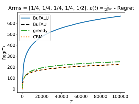
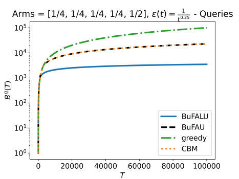
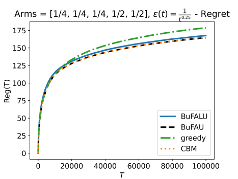
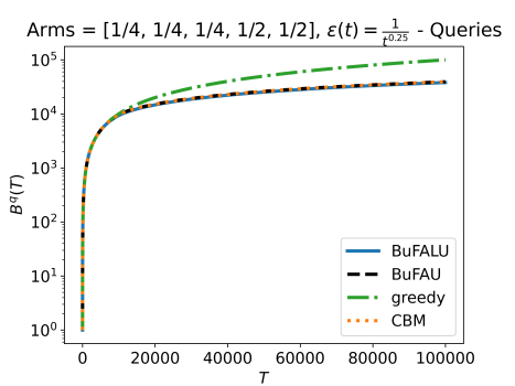
Figure 2: Evaluation of all algorithms on 5-armed problems over $1,000$ seeds with $\epsilon(t)=t^{-1/4}$.

Table 2: Additional statistics of the empirical evaluation in Figure 2. All statistics are measured after $T=100,000$ time steps over $1,000$ different seeds. All experiments use $\epsilon(t)=t^{-1/4}$. std is the standard deviation, $90\%$ represents the $90^{th}$ percentile and max is the maximum.

		Regret				Queries
Bandit Instance	Algorithm	mean	std	$90\%$	max	mean	std	$90\%$	max
	BuFALU	664.88	87.08	774.8	982.25	3471.38	437.39	4024.1	5023
	BuFAU	222.94	23.03	253.25	304.5	22736.7	92.1	22858	23063
	greedy	248.08	26.18	281.77	343.75	100000	0	100000	100000
5-arms, unique optimal, values: $\left[\frac{1}{4},\frac{1}{4},\frac{1}{4},\frac{1}{4},\frac{1}{2}\right]$	CBM	222.97	23.06	253.25	304.5	22736.9	92.25	22858	23063
	BuFALU	167.64	20.17	194.52	230.75	38049.3	3944.21	42593.5	44135
	BuFAU	164.62	19.75	190.02	230.25	39254.9	3292.47	43298.1	44383
	greedy	178.79	21.72	207.78	256.75	100000	0	100000	100000
5-arms, multiple optimal, values: $\left[\frac{1}{4},\frac{1}{4},\frac{1}{4},\frac{1}{2},\frac{1}{2}\right]$	CBM	164.92	19.95	190.5	245	39217.6	3277.71	43289.4	44383

For completeness, we also present simulation results for two additional profiles of $\epsilon(t)$ – the first is when $\epsilon(t)=0$ (see Figure 3 and statistics in Table 3) and the second when $\epsilon(t)=\frac{1}{\ln t}$ (see Figure 4 and statistics in Table 4). When $\epsilon(t)=0$, algorithms are allowed to ask as much feedback as they want. Then, when there are multiple optimal arms, all algorithms always ask for feedback and perform the same. On the other hand, when the optimal arm is unique, BuFALU asks for feedback on $\sim\frac{1}{20}$ of the rounds and suffers a factor of $4$ in its regret. Therefore, in the unlimited budget scenario, we return to the same behavior as in Section 5.2. The case of $\epsilon(t)=\frac{1}{\ln t}$, which corresponds to a querying budget of $\mathcal{O}(K\ln^{3}t)$, behaves very similar to the choice of $\epsilon(t)=t^{-1/4}$. Interestingly, when the optimal arm is unique, the regret of BuFALU in both limited cases is lower than the regret when $\epsilon(t)=0$. A possible explanation is that when the budget is unlimited, BuFALU aggressively explores to separate the optimal arm from all other arms. When the budget is limited, BuFALU combines exploration with exploitation of $l_{t}$, which leads to a slightly lower regret.

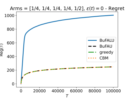
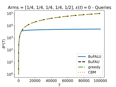
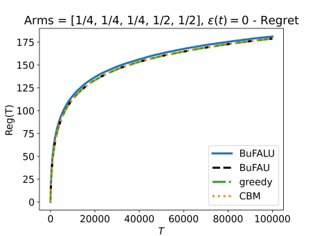
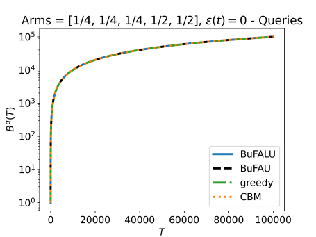
Figure 3: Evaluation of all algorithms on 5-armed problems over $1,000$ seeds with $\epsilon(t)=0$.

Table 3: Additional statistics of the empirical evaluation in Figure 3. All statistics are measured after $T=100,000$ time steps over $1,000$ different seeds. All experiments use $\epsilon(t)=0$. std is the standard deviation, $90\%$ represents the $90^{th}$ percentile and max is the maximum.

		Regret				Queries
Bandit Instance	Algorithm	mean	std	$90\%$	max	mean	std	$90\%$	max
	BuFALU	1003.96	131.23	1180.55	1457.25	5240.73	658.93	6130	7538
	BuFAU	248.08	26.18	281.77	343.75	100000	0	100000	100000
	greedy	248.08	26.18	281.77	343.75	100000	0	100000	100000
5-arms, unique optimal, values: $\left[\frac{1}{4},\frac{1}{4},\frac{1}{4},\frac{1}{4},\frac{1}{2}\right]$	CBM	248.08	26.18	281.77	343.75	100000	0	100000	100000
	BuFALU	181.05	21.6	208.02	259.5	100000	0	100000	100000
	BuFAU	178.79	21.72	207.78	256.75	100000	0	100000	100000
	greedy	178.79	21.72	207.78	256.75	100000	0	100000	100000
5-arms, multiple optimal, values: $\left[\frac{1}{4},\frac{1}{4},\frac{1}{4},\frac{1}{2},\frac{1}{2}\right]$	CBM	178.79	21.72	207.78	256.75	100000	0	100000	100000

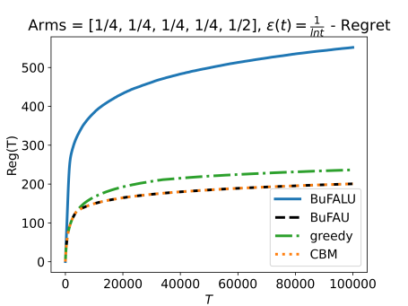
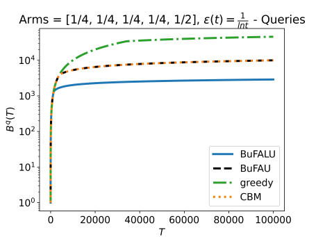
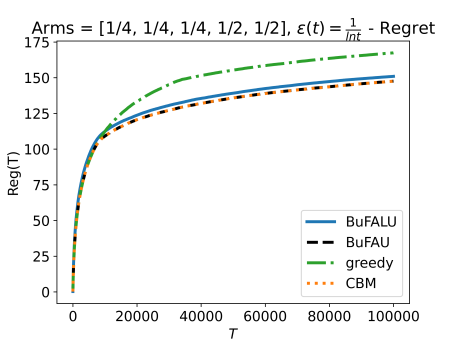
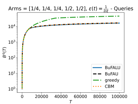
Figure 4: Evaluation of all algorithms on 5-armed problems over $1,000$ seeds with $\epsilon(t)=\frac{1}{\ln t}$.

Table 4: Additional statistics of the empirical evaluation in Figure 4. All statistics are measured after $T=100,000$ time steps over $1,000$ different seeds. All experiments use $\epsilon(t)=\frac{1}{\ln t}$. std is the standard deviation, $90\%$ represents the $90^{th}$ percentile and max is the maximum.

		Regret				Queries
Bandit Instance	Algorithm	mean	std	$90\%$	max	mean	std	$90\%$	max
	BuFALU	551.43	73.82	644.08	780.25	2881.58	373.37	3336.5	4072
	BuFAU	200.47	21.92	228.75	276.25	9958.88	87.68	10072	10262
	greedy	236.37	24.63	269.02	311.5	45785	0	45785	45785
5-arms, unique optimal, values: $\left[\frac{1}{4},\frac{1}{4},\frac{1}{4},\frac{1}{4},\frac{1}{2}\right]$	CBM	200.52	21.94	228.82	276.25	9959.06	87.76	10072.3	10262
	BuFALU	150.97	17.9	173.78	210	16349.9	1762.22	18277.3	18954
	BuFAU	147.59	18.04	170	235.5	16811.8	1387.87	18504.5	19022
	greedy	167.42	20.59	194.02	238.25	45785	0	45785	45785
5-arms, multiple optimal, values: $\left[\frac{1}{4},\frac{1}{4},\frac{1}{4},\frac{1}{2},\frac{1}{2}\right]$	CBM	147.57	17.99	170.5	235.5	16827.3	1390.31	18523.1	19022

C.2.2 Testing the Effect of the Total Budget

We now test the effect of the total budget on the regret and number of feedback queries. We do so problems with Bernoulli arms, optimal arm $\mu^{*}=0.5$, a single suboptimal arm $\mu_{a}=0.25$ and either a unique or two optimal arms (namely, two and three-armed problems, respectively). The time horizon in the simulations is $T=1,000$ and results were averaged over $1,000$ seeds. To simulate the effect of the total budget, we allocated a fixed budget $B$ throughout the interactions (i.e., set $\epsilon(t)=\sqrt{\frac{6K\ln t}{B}}$) and measured both the regret and number of queries at the last time step, as a function of the (fractional) allocated budget $B/T$. The results are depicted in Figure 5, and error bars represent a variation of one standard deviation.

Interestingly, the regret first decreases, achieves a minimum when $B/T\approx 0.08$, and then starts increasing. We believe that this is since the standard UCB bounds are a little loose and can be replaced by [Garivier and Cappé, 2011]:

$$UCB_{t}(a)=\hat{\mu}_{t-1}\left(a\right)+\sqrt{\frac{\ln t+3\ln\ln t}{2n^{q}_{t-1}\left(a\right)}}\enspace.$$

Therefore, the algorithm suffers from some over-exploration. Then, the local minimum of the regret allocates enough budget to adequately explore and then forces the algorithm the exploit, which leads to a better exploration-exploitation tradeoff.

Asides from this phenomenon, the graph behaves as could be expected. As we previously saw, all algorithms achieve roughly the same performance in the presence of multiple optimal arms. When the optimal arm is unique, BuFALU is substantially fewer budget queries but suffers from a small regret degradation (up to a factor of $4$). Notably, in the small-budget regime, BuFALU achieves similar regret to all other baselines.

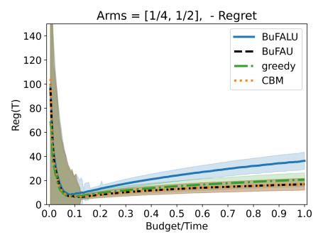
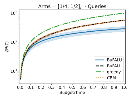
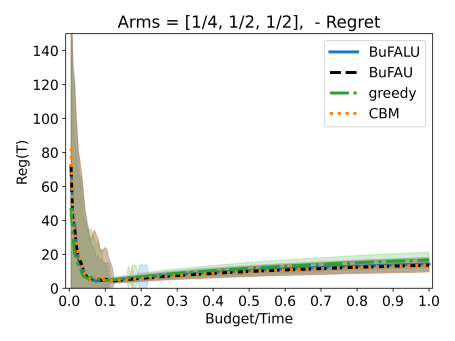
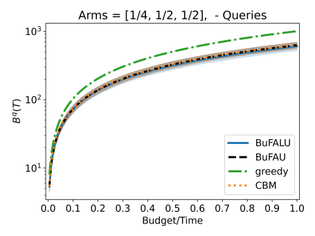
Figure 5: Regret and Queries as a function of the allocated budget in two and three armed bandit problems.

References

- Abbasi-Yadkori et al. [2011] Yasin Abbasi-Yadkori, Dávid Pál, and Csaba Szepesvári. Improved algorithms for linear stochastic bandits. In Advances in Neural Information Processing Systems, pages 2312–2320, 2011.
- Azar et al. [2013] Mohammad Gheshlaghi Azar, Rémi Munos, and Hilbert J Kappen. Minimax pac bounds on the sample complexity of reinforcement learning with a generative model. Machine learning, 91(3):325–349, 2013.
- Badanidiyuru et al. [2013] Ashwinkumar Badanidiyuru, Robert Kleinberg, and Aleksandrs Slivkins. Bandits with knapsacks. In 2013 IEEE 54th Annual Symposium on Foundations of Computer Science, pages 207–216. IEEE, 2013.
- Bubeck et al. [2012] Sébastien Bubeck, Nicolo Cesa-Bianchi, et al. Regret analysis of stochastic and nonstochastic multi-armed bandit problems. Foundations and Trends® in Machine Learning, 5(1):1–122, 2012.
- Burnetas and Katehakis [1996] Apostolos N Burnetas and Michael N Katehakis. Optimal adaptive policies for sequential allocation problems. Advances in Applied Mathematics, 17(2):122–142, 1996.
- Chen et al. [2016a] Wei Chen, Yajun Wang, Yang Yuan, and Qinshi Wang. Combinatorial multi-armed bandit and its extension to probabilistically triggered arms. The Journal of Machine Learning Research, 17(1):1746–1778, 2016a.
- Efroni et al. [2021] Yonathan Efroni, Nadav Merlis, Aadirupa Saha, and Shie Mannor. Confidence-budget matching for sequential budgeted learning. arXiv preprint arXiv:2102.03400, 2021.
- Gabillon et al. [2012] Victor Gabillon, Mohammad Ghavamzadeh, and Alessandro Lazaric. Best arm identification: A unified approach to fixed budget and fixed confidence. In Advances in Neural Information Processing Systems, pages 3212–3220, 2012.
- Garivier and Cappé [2011] Aurélien Garivier and Olivier Cappé. The kl-ucb algorithm for bounded stochastic bandits and beyond. In Proceedings of the 24th annual conference on learning theory, pages 359–376, 2011.
- Garivier et al. [2018] Aurélien Garivier, Hédi Hadiji, Pierre Menard, and Gilles Stoltz. Kl-ucb-switch: optimal regret bounds for stochastic bandits from both a distribution-dependent and a distribution-free viewpoints. arXiv preprint arXiv:1805.05071, 2018.
- Garivier et al. [2019] Aurélien Garivier, Pierre Ménard, and Gilles Stoltz. Explore first, exploit next: The true shape of regret in bandit problems. Mathematics of Operations Research, 44(2):377–399, 2019.
- Jaksch et al. [2010] Thomas Jaksch, Ronald Ortner, and Peter Auer. Near-optimal regret bounds for reinforcement learning. Journal of Machine Learning Research, 11(Apr):1563–1600, 2010.
- Kalyanakrishnan et al. [2012] Shivaram Kalyanakrishnan, Ambuj Tewari, Peter Auer, and Peter Stone. Pac subset selection in stochastic multi-armed bandits. In ICML, volume 12, pages 655–662, 2012.
- Lai and Robbins [1985] Tze Leung Lai and Herbert Robbins. Asymptotically efficient adaptive allocation rules. Advances in applied mathematics, 6(1):4–22, 1985.
- Lykouris et al. [2018] Thodoris Lykouris, Vahab Mirrokni, and Renato Paes Leme. Stochastic bandits robust to adversarial corruptions. In Proceedings of the 50th Annual ACM SIGACT Symposium on Theory of Computing, pages 114–122, 2018.
- Maurer and Pontil [2009] Andreas Maurer and Massimiliano Pontil. Empirical bernstein bounds and sample variance penalization. arXiv preprint arXiv:0907.3740, 2009.
- Merlis and Mannor [2020] Nadav Merlis and Shie Mannor. Lenient regret for multi-armed bandits. arXiv preprint arXiv:2008.03959, 2020.
- Pike-Burke et al. [2018] Ciara Pike-Burke, Shipra Agrawal, Csaba Szepesvari, and Steffen Grunewalder. Bandits with delayed, aggregated anonymous feedback. In International Conference on Machine Learning, pages 4105–4113. PMLR, 2018.
- Robbins [1952] Herbert Robbins. Some aspects of the sequential design of experiments. Bulletin of the American Mathematical Society, 58(5):527–535, 1952.
- Seldin et al. [2014] Yevgeny Seldin, Peter Bartlett, Koby Crammer, and Yasin Abbasi-Yadkori. Prediction with limited advice and multiarmed bandits with paid observations. In International Conference on Machine Learning, pages 280–287. PMLR, 2014.
- Simchowitz and Jamieson [2019] Max Simchowitz and Kevin G Jamieson. Non-asymptotic gap-dependent regret bounds for tabular mdps. In Advances in Neural Information Processing Systems, volume 32, 2019.
- Tirinzoni et al. [2021] Andrea Tirinzoni, Matteo Pirotta, and Alessandro Lazaric. A fully problem-dependent regret lower bound for finite-horizon mdps. arXiv preprint arXiv:2106.13013, 2021.
- Xu et al. [2021] Haike Xu, Tengyu Ma, and Simon S Du. Fine-grained gap-dependent bounds for tabular mdps via adaptive multi-step bootstrap. arXiv preprint arXiv:2102.04692, 2021.
- Yun et al. [2018] Donggyu Yun, Alexandre Proutiere, Sumyeong Ahn, Jinwoo Shin, and Yung Yi. Multi-armed bandit with additional observations. Proceedings of the ACM on Measurement and Analysis of Computing Systems, 2(1):1–22, 2018.