Action-Sufficient State Representation Learning for Control with Structural Constraints

Abstract

Perceived signals in real-world scenarios are usually high-dimensional and noisy, and finding and using their representation that contains essential and sufficient information required by downstream decision-making tasks will help improve computational efficiency and generalization ability in the tasks. In this paper, we focus on partially observable environments and propose to learn a minimal set of state representations that capture sufficient information for decision-making, termed Action-Sufficient state Representations (ASRs). We build a generative environment model for the structural relationships among variables in the system and present a principled way to characterize ASRs based on structural constraints and the goal of maximizing cumulative reward in policy learning. We then develop a structured sequential Variational Auto-Encoder to estimate the environment model and extract ASRs. Our empirical results on CarRacing and VizDoom demonstrate a clear advantage of learning and using ASRs for policy learning. Moreover, the estimated environment model and ASRs allow learning behaviors from imagined outcomes in the compact latent space to improve sample efficiency.

1 Introduction

State-of-the-art reinforcement learning (RL) algorithms leveraging deep neural networks are usually data hungry and lack interpretability. For example, to attain expert-level performance on tasks such as chess or Atari games, deep RL systems usually require many orders of magnitude more training data than human experts (Tsividis et al., 2017). One of the reasons is that our perceived signals in real-world scenarios, e.g., images, are usually high-dimensional and may contain much irrelevant information for decision-making of the task at hand. This makes it difficult and expensive for an agent to directly learn optimal policies from raw observational data. Fortunately, the underlying states that directly guide decision-making could be much lower-dimensional (Schölkopf, 2019; Bengio, 2019). One example is that when crossing the street, our decision on when to cross relies on the traffic lights. The useful state of traffic lights (e.g., its color) can be represented by a single binary variable, while the perceived image is high-dimensional. It is essential to extract and exploit such lower-dimensional states to improve the efficiency and interpretability of the decision-making process.

Recently, representation learning algorithms have been designed to learn abstract features from high-dimensional and noisy observations. Exploiting the abstract representations, instead of the raw data, has been shown to perform subsequent decision-making more efficiently (Lesort et al., 2018). Representative methods along this line include deep Kalman filters (Krishnan et al., 2015), deep variational Bayes filters (Karl et al., 2016), world models (Ha & Schmidhuber, 2018), PlaNet (Hafner et al., 2018), DeepMDP (Gelada et al., 2019), stochastic latent actor-critic (Lee et al., 2019), SimPLe (Kaiser et al., 2019), Bisimulation-based methods (Zhang et al., 2021), Dreamer (Hafner et al., 2019, 2020), and others (Srinivas et al., 2020; Shu et al., 2020). Moreover, if we can properly model and estimate the underlying transition dynamics, then we can perform model-based RL or planning, which can effectively reduce interactions with the environment (Ha & Schmidhuber, 2018; Hafner et al., 2018, 2019, 2020).

Despite the effectiveness of the above approaches to learning abstract features, current approaches usually fail to take into account whether the extracted state representations are sufficient and necessary for downstream policy learning. State representations that contain insufficient information may lead to sub-optimal policies, while those with redundant information may require more samples and more complex models for training. We address this problem by modeling the generative process and selection procedure induced by reward maximization; by considering a generative environment model involving observed states, state-transition dynamics, and rewards, and explicitly characterizing structural relationships among variables in the RL system, we propose a principled approach to learning minimal sufficient state representations. We show that only the state dimensions that have direct or indirect edges to the reward variable are essential and should be considered for decision making. Furthermore, they can be learned by maximizing their ability to predict the action, given that the cumulative reward is included in the prediction model, while at the same time achieving their minimality w.r.t. the mutual information with observations as well as their dimensionality. The contributions of this paper are summarized as follows:

• We construct a generative environment model, which includes the observation function, transition dynamics, and reward function, and explicitly characterizes structural relationships among variables in the RL system.

• We characterize a minimal sufficient set of state representations, termed Action-Sufficient state Representations (ASRs), for the downstream policy learning by making use of structural constraints and the goal of maximizing cumulative reward in policy learning.

• In light of the characterization, we develop Structured Sequential Variational Auto-Encoder (SS-VAE), which explicitly encodes structural relationships among variables, for reliable identification of ASRs.

• Accordingly, policy learning can be done separately from representation learning, and the policy function only relies on a set of low-dimensional state representations, which improve both model and sample efficiency. Moreover, the estimated environment model and ASRs allow learning behaviors from imagined outcomes in the compact latent space, which effectively reduce possibly risky explorations.

2 Environment Model with Structural Constraints

In order to characterize a set of minimal sufficient state representations for downstream policy learning, we first formulate a generative environment model in partially observable Markov decision process (POMDP), and then show how to explicitly embed structural constraints over variables in the RL system and leverage them.

Suppose we have sequences of observations $\{\langle o_{t},a_{t},r_{t}\rangle\}_{t=1}^{T}$, where $o_{t}\in\mathcal{O}$ denotes perceived signals at time $t$, such as high-dimensional images, with $\mathcal{O}$ being the observation space, $a_{t}\in\mathcal{A}$ is the performed action with $\mathcal{A}$ being the action space, and $r_{t}\in\mathcal{R}$ represents the reward variable with $\mathcal{R}$ being the reward space. We denote the underlying states, which are latent, by $\vec{s}_{t}\in\mathcal{S}$, with $\mathcal{S}$ being the state space. We describe the generating process of the environment model as follows:

$$\left\{\begin{array}[]{lll}o_{t}=f(\vec{s}_{t},e_{t}),\\ r_{t}=g(\vec{s}_{t-1},a_{t-1},\epsilon_{t}),\\ \vec{s}_{t}=h(\vec{s}_{t-1},a_{t-1},\eta_{t}),\end{array}\right.$$ (1)

where $f$, $g$, and $h$ represent the observation function, reward function, and transition dynamics, respectively, and $e_{t}$, $\epsilon_{t}$, and $\eta_{t}$ are corresponding independent and identically distributed (i.i.d.) random noises. The latent states $\vec{s}_{t}$ form an MDP: given $\vec{s}_{t-1}$ and $a_{t-1}$, $\vec{s}_{t}$ are independent of states and actions before $t-1$. Moreover, the action $a_{t-1}$ directly influences latent states $\vec{s}_{t}$, instead of perceived signals $o_{t}$, and the reward is determined by the latent states (and the action) as well. The perceived signals $o_{t}$ are generated from the underlying states $\vec{s}_{t}$, contaminated by random noise $e_{t}$. We also consider noise $\epsilon_{t}$ in the reward function to capture unobserved factors that may affect the reward, as well as measurement noise.

It is commonplace that the action variable $a_{t-1}$ may not influence every dimension of $\vec{s}_{t}$, and the reward $r_{t}$ may not be influenced by every dimension of $\vec{s}_{t-1}$ as well, and furthermore there are structural relationships among different dimensions of $\vec{s}_{t}$. Figure 1 gives an illustrative graphical representation, where $s_{3,t-1}$ influences $s_{2,t}$, $a_{t-1}$ does not have an edge to $s_{3,t}$, and among the states, only $s_{2,t-1}$ and $s_{3,t-1}$ have edges to $r_{t}$. We use $R_{t}=\sum_{\tau=t}^{\infty}\gamma^{\tau-t}r_{\tau}$ to denote the discounted cumulative reward starting from time $t$, where $\gamma\in[0,1]$ is the discounted factor that determines how much immediate rewards are favored over more distant rewards.

To reflect such constraints, we explicitly encode the graph structure over variables, including the structure over different dimensions of $\vec{s}$ and the structures from $a_{t-1}$ to $\vec{s}_{t}$, $\vec{s}_{t-1}$ to $r_{t}$, and $\vec{s}_{t}$ to $o_{t}$. Accordingly, we re-formulate (1) as follows:

$$\left\{\begin{array}[]{lll}o_{t}=f(D_{\vec{s}{\hbox{\rule[0.0pt]{0.0pt}{0.0pt}}\mkern-4.0mu\hbox{\char 41\relax}}o}\odot\vec{s}_{t},e_{t}),\\ r_{t}=g(D_{\vec{s}{\hbox{\rule[0.0pt]{0.0pt}{0.0pt}}\mkern-4.0mu\hbox{\char 41\relax}}r}\odot\vec{s}_{t-1},D_{a{\hbox{\rule[0.0pt]{0.0pt}{0.0pt}}\mkern-4.0mu\hbox{\char 41\relax}}r}\odot a_{t-1},\epsilon_{t}),\\ s_{i,t}=h_{i}(D_{\vec{s}(\cdot,i)}\odot\vec{s}_{t-1},D_{a{\hbox{\rule[0.0pt]{0.0pt}{0.0pt}}\mkern-4.0mu\hbox{\char 41\relax}}\vec{s}(\cdot,i)}\odot a_{t-1},\eta_{i,t}),\end{array}\right.$$ (2)

for $i=1,\cdots,d$, where $\vec{s}_{t}=(s_{1,t},\cdots,s_{d,t})^{\top}$, $\odot$ denotes element-wise product, and $D_{(\cdot)}$ are binary matrices indicating the graph structure over variables. Specifically, $D_{\vec{s}{\hbox{\rule[0.0pt]{0.0pt}{0.0pt}}\mkern-4.0mu\hbox{\char 41\relax}}o}\in\{0,1\}^{d\times 1}$ represents the graph structure from $d$-dimensional $\vec{s}_{t}$ to $o_{t}$, $D_{\vec{s}{\hbox{\rule[0.0pt]{0.0pt}{0.0pt}}\mkern-4.0mu\hbox{\char 41\relax}}r}\in\{0,1\}^{d\times 1}$ the structure from $\vec{s}_{t-1}$ to the reward variable $r_{t}$, $D_{a{\hbox{\rule[0.0pt]{0.0pt}{0.0pt}}\mkern-4.0mu\hbox{\char 41\relax}}r}\in\{0,1\}$ the structure from the action variable $a_{t-1}$ to the reward variable $r_{t}$, $D_{\vec{s}}\in\{0,1\}^{d\times d}$ denotes the graph structure from $d$-dimensional $\vec{s}_{t-1}$ to $d$-dimensional $\vec{s}_{t}$ and $D_{\vec{s}(\cdot,i)}$ is its $i$-th column, and $D_{a{\hbox{\rule[0.0pt]{0.0pt}{0.0pt}}\mkern-4.0mu\hbox{\char 41\relax}}\vec{s}}\in\{0,1\}^{1\times d}$ corresponds to the graph structure from $a_{t-1}$ to $\vec{s}_{t}$ with $D_{a{\hbox{\rule[0.0pt]{0.0pt}{0.0pt}}\mkern-4.0mu\hbox{\char 41\relax}}\vec{s}(\cdot,i)}$ representing its $i$-th column. For example, $D_{\vec{s}(j,i)}=0$ means that there is no edge from $s_{j,t-1}$ to $s_{i,t}$. Here, we assume that the environment model, as well as the structural constraints, is invariant across time instance $t$.

Figure 1: A graphical illustration of the generative environment model. Grey nodes denote observed variables and white nodes represent unobserved variables. Here, $a_{t-1}$ does not have an edge to $s_{3,t}$, and only $s_{2,t-1}$ and $s_{3,t-1}$ have edges to $r_{t}$, and moreover, we take into account the structural relationships among different dimensions of latent states $\vec{s}_{t}$. The solid lines represent causal relations, while the dashed lines represent predictions of $a_{t}$ from $\vec{s}_{t}$, which is not causal, and moreover, dashed lines mean that the relations may not exist and they may differ under different policies.

2.1 Minimal Sufficient State Representations

Given observational sequences $\{\langle o_{t},a_{t},r_{t}\rangle\}_{t=1}^{T}$, we aim to learn minimal sufficient state representations for the downstream policy learning. In the following, we first characterize the state dimensions that are indispensable for policy learning, when the environment model, including structural relationships, is given. Then we provide criteria to achieve sufficiency and minimality of the estimated state representations, when only $\{\langle o_{t},a_{t},r_{t}\rangle\}_{t=1}^{T}$, but not the environment model, is given.

Finding minimal sufficient state dimensions with a given environment model.

RL agents learn to choose appropriate actions according to the current state vector $\vec{s}_{t}$ to maximize the future cumulative reward, in which some dimensions may be redundant for policy learning. Then how can we identify a minimal subset of state dimensions that are sufficient to choose optimal actions? Below, we first give the definition of Action-Sufficient state Representations (ASRs) according to the graph structure. We further show in Proposition 1 that ASRs are minimal sufficient for policy learning, and they can be characterized by leveraging the (conditional) independence/dependence relations among the quantities, under the Markov condition and faithfulness assumption (Pearl, 2000; Spirtes et al., 1993).

Definition 1 (Action-Sufficient State Representations (ASRs)).

Given the graphical representation corresponding to the environment model, such as the representation in Figure 1, we define recursively ASRs that affect the future reward as: (1) $s_{i,t}\in\vec{s}_{t}^{\,\text{ASR}}$ has an edge to the reward in the next time-step $r_{t+1}$, or (2) $s_{i,t}\in\vec{s}_{t}^{\,\text{ASR}}$ has an edge to another state dimension in the next time-step $s_{j,t+1}$, such that the same component at time $t$ is in ASRs, i.e., $s_{j,t}\in\vec{s}_{t}^{\,\text{ASR}}$.

Proposition 1.

Under the assumption that the graphical representation, corresponding to the environment model, is Markov and faithful to the measured data, $\vec{s}_{t}^{\,\text{ASR}}\subseteq\vec{s}_{t}$ are a minimal subset of state dimensions that are sufficient for policy learning, and $s_{i,t}\in\vec{s}_{t}^{\,\text{ASR}}$ if and only if $s_{i,t}\not\!\perp\!\!\!\perp R_{t+1}|a_{t-1:t},\vec{s}_{t-1}^{\,\text{ASR}}$.

Proposition 1 can be shown based on the global Markov condition and the faithfulness assumption, which connects d-separation to conditional independence/dependence relations. A proof is given in Appendix. According to the above proposition, it is easy to see that for the graph given in Figure 1, we have $\vec{s}_{t}^{\,\text{ASR}}=(s_{2,t},s_{3,t})^{\top}$. That is, we only need $(s_{2,t},s_{3,t})^{\top}$, instead of $\vec{s}_{t}$, for the downstream policy learning.

Minimal sufficient state representation learning from observed sequences.

In practice, we usually do not have access to the latent states or the environment model, but instead only the observed sequences $\{\langle o_{t},a_{t},r_{t}\rangle\}_{t=1}^{T}$. Then how can we learn the ASRs from the raw high-dimensional inputs such as images? We denote by $\tilde{\vec{s}}_{t}$ the estimated whole latent state representations and $\tilde{\vec{s}}_{t}^{\,\text{ASR}}\subseteq\tilde{\vec{s}}_{t}$ the estimated minimal sufficient state representations for policy learning.

As discussed above, ASRs and $R_{t+1}$ are dependent given $a_{t-1:t}$ and $\tilde{\vec{s}}_{t-1}^{\,\text{ASR}}$, while other state dimensions are independent of $R_{t+1}$, so we can learn the ASRs by maximizing

$$\leavevmode\resizebox{399.2946pt}{}{$I(\tilde{\vec{s}}^{\,\text{ASR}};R_{t+1}|a_{t-1:t},\tilde{\vec{s}}_{t-1}^{\,\text{ASR}})-I(\tilde{\vec{s}}^{\,\text{C}};R_{t+1}|a_{t-1:t},\tilde{\vec{s}}_{t-1}^{\,\text{ASR}})$},$$ (3)

where $\tilde{\vec{s}}^{\,\text{C}}=\tilde{\vec{s}}\backslash\tilde{\vec{s}}^{\,\text{ASR}}$, and $I(\cdot)$ denotes mutual information. Such regularization is used to achieve minimal sufficient state representations for policy learning; that is, only $\tilde{\vec{s}}_{t-1}^{\,\text{ASR}}$ are useful for policy learning, while $\tilde{\vec{s}}_{t-1}^{\,\text{C}}$ are not. Furthermore, the mutual information can be represented as a form of conditional entropy, e.g., $I(\tilde{\vec{s}}^{\,\text{ASR}};R_{t+1}|a_{t-1:t},\vec{s}_{t-1}^{\,\text{ASR}})=H(\tilde{\vec{s}}^{\,\text{ASR}}|a_{t-1:t},\vec{s}_{t-1}^{\,\text{ASR}})-H(\tilde{\vec{s}}^{\,\text{ASR}}|R_{t+1},a_{t-1:t},\vec{s}_{t-1}^{\,\text{ASR}})$, where $H(\cdot)$ denotes the conditional entropy, with

$$\begin{array}[]{lll}\footnotesize&H(\tilde{\vec{s}}^{\,\text{ASR}}|a_{t-1:t},\tilde{\vec{s}}_{t-1}^{\,\text{ASR}})\\ &=\!-\mathbb{E}_{q_{\phi}}\mathbb{E}_{p_{\alpha_{1}}}\!\big{\{}\!\log p_{\alpha_{1}}(\tilde{\vec{s}}^{\text{ASR}}|a_{t-1:t},\tilde{\vec{s}}_{t-1}^{\,\text{ASR}})\!\big{\}}\\ &=\!-\mathbb{E}_{q_{\phi}}\mathbb{E}_{p_{\alpha_{1}}}\!\big{\{}\!\log p_{\alpha_{1}}(\tilde{\vec{s}}^{\text{ASR}}|a_{t-1:t},\tilde{D}^{ASR}\odot\tilde{\vec{s}}_{t-1})\!\big{\}}\!,\end{array}$$

and

$$\begin{array}[]{lll}\footnotesize&H(\tilde{\vec{s}}^{\,\text{ASR}}|R_{t+1},a_{t-1:t},\tilde{\vec{s}}_{t-1}^{\,\text{ASR}})\\ &\!\!\!\!\!=\!-\mathbb{E}_{q_{\phi}}\mathbb{E}_{p_{\alpha_{2}}}\!\big{\{}\!\log p_{\alpha_{2}}(\tilde{\vec{s}}^{\text{ASR}}|R_{t+1},a_{t-1:t},\tilde{D}^{ASR}\odot\tilde{\vec{s}}_{t-1})\!\big{\}},\\ \end{array}$$

where $p_{\alpha_{i}}$, for $i=1,2$, denotes the probabilistic predictive model of $\tilde{\vec{s}}^{\,\text{ASR}}$ with parameters $\alpha_{i}$, and $q_{\phi}(\tilde{\vec{s}}_{t}|\tilde{\vec{s}}_{t-1},\mathbf{y}_{1:t},a_{1:t-1})$ is the probabilistic inference model of $\tilde{\vec{s}}_{t}$ with parameters $\phi$ and $\mathbf{y}_{t}\!=\!(o_{t}^{T},r_{t}^{T})$, and $\tilde{D}^{\,\text{ASR}}\in\{0,1\}^{\tilde{d}\times 1}$ is a binary vector indicating which dimensions of $\tilde{\vec{s}}_{t}$ are in $\tilde{\vec{s}}_{t}^{\,\text{ASR}}$, so $\tilde{D}^{\,\text{ASR}}\odot\tilde{\vec{s}}_{t}$ gives ASRs $\tilde{\vec{s}}_{t}^{\,\text{ASR}}$. Similarly, we can also represent $I(\tilde{\vec{s}}^{\,\text{C}};R_{t+1}|a_{t-1:t},\tilde{\vec{s}}_{t-1}^{\,\text{ASR}})$ in such a way.

Although with the above regularization, we can achieve ASRs theoretically, in practice, we further add another regularization to achieve minimality of the representation by minimizing conditional mutual information between observed high-dimensional signals $\mathbf{y}_{t}$ and the ASR $\tilde{\vec{s}}_{t}^{\,\text{ASR}}$ at time $t$ given data at previous time instances, similar to that in information bottleneck (Tishby et al., 1999), and meanwhile minimizing the dimensionality of ASRs with sparsity constraints:

$$\lambda_{1}\sum\nolimits_{t=2}^{T}I(\mathbf{y}_{t};\tilde{\vec{s}}_{t}^{\,\text{ASR}}|\mathbf{y}_{1:t-1},a_{1:t-1},\tilde{\vec{s}}_{t-1})+\lambda_{2}\|\tilde{D}^{\,\text{ASR}}\|_{1},$$

where the conditional mutual information can be upper bound by a KL-divergence:

$$I(\mathbf{y}_{t};\tilde{\vec{s}}_{t}^{\,\text{ASR}}|\mathbf{y}_{1:t-1},a_{1:t-1},\tilde{\vec{s}}_{t-1})\leq\mathbb{E}\big{\{}\text{KL}\big{(}q_{\phi^{\prime}}\|p_{\gamma}\big{)}\big{\}},$$ (4)

with $q_{\phi^{\prime}}\equiv q_{\phi^{\prime}}(\tilde{\vec{s}}_{t}^{\,\text{ASR}}|\tilde{\vec{s}}_{t-1},\mathbf{y}_{1:t},a_{1:t-1})$ and $p_{\gamma}\equiv p_{\gamma}(\tilde{\vec{s}}_{t}^{\,\text{ASR}}|\tilde{\vec{s}}_{t-1},a_{t-1};D_{\vec{s}},D_{a{\hbox{\rule[0.0pt]{0.0pt}{0.0pt}}\mkern-4.0mu\hbox{\char 41\relax}}\vec{s}})$ being the transition dynamics of $\tilde{\vec{s}}_{t}$ with parameters $\gamma$, and the expectation is over $p(\tilde{\vec{s}}_{t-1},\mathbf{y}_{1:t},a_{1:t-1})$.

Furthermore, Proposition 1 shows that given the (estimated) environment model, only those state dimensions that have a directed path to the reward variable are the ASRs. In our learning procedure, we also take into account the relationship between the learned states $\tilde{\vec{s}}_{t}$ and the reward, and leverage such structural constraints for learning the ASRs. Denote by $\check{D}^{ASR}\in\{0,1\}^{\tilde{d}\times 1}$ a binary vector indicating whether the corresponding state dimension in $\tilde{\vec{s}}_{t}$ has a directed path to the reward variable. Consequently, we enforce the similarity between $\check{D}^{ASR}$ and $\tilde{D}^{ASR}$ by adding an $L_{1}$ norm on $\check{D}^{ASR}-\tilde{D}^{ASR}$. Therefore, the ASRs can be learned by maximizing the following function:

$$\small\begin{array}[]{lll}\mathcal{L}^{\text{min \& suff}}=\\ \!\!\!\!\lambda_{3}\!\underbrace{\sum\nolimits_{t=1}^{T}\!\!\big{\{}I(\tilde{\vec{s}}^{\,\text{ASR}}\!;R_{t+1}|a_{t-1:t},\tilde{\vec{s}}_{t-1}^{\,\text{ASR}})\!-\!I(\tilde{\vec{s}}^{\,\text{C}}\!;R_{t+1}|a_{t-1:t},\tilde{\vec{s}}_{t-1}^{\,\text{ASR}})\!\big{\}}}_{\text{Sufficiency \& Minimality}}\\ \!\!\!\!-\lambda_{4}\|\check{D}_{\,\text{ASR}}\!-\!\tilde{D}_{\,\text{ASR}}\|_{1}\!\!\underbrace{-\!\lambda_{1}\sum_{t=1}^{T}\mathbb{E}\big{\{}\text{KL}\big{(}q_{\phi}\|p_{\gamma}\big{)}\big{\}}\!-\!\lambda_{2}\|\tilde{D}^{ASR}\|_{1}}_{\text{Further restrictions of minimality}},\end{array}$$ (5)

where $\lambda$’s are regularization terms, and note that $\check{D}^{ASR}$ can be directly derived from the estimated structural matrices $D_{a{\hbox{\rule[0.0pt]{0.0pt}{0.0pt}}\mkern-4.0mu\hbox{\char 41\relax}}r}\text{ and }D_{\vec{s}(\cdot,i)}$. The constraint in Eq. 5 provides a principled way to achieve minimal sufficient state representations. Notice that it is just part of the objective function to maximize, and it will be involved in the complete objective function in Fig. 2 to learn the whole environment model.

Remarks.

By explicitly involving structural constraints, we achieve minimal sufficient state representations from the view of generative process underlying the RL problem and the selection procedure induced by reward maximization, which enjoys the following advantages. 1) The structural information provides an interpretable and intuitive picture of the generating process. 2) Accordingly, it also provides an interpretable and intuitive way to characterize a minimal sufficient set of state representations for policy learning, which removes unrelated information. 3) There is no information loss when representation learning and policy learning are done separately, which is computationally more efficient. 4) The generative environment model is fixed, independent of the behavior policy that is performed. Furthermore, based on the estimated environment model and ASRs, it is flexible to use a wide range of policy learning methods, and one can also perform model-based RL, which effectively reduce possibly risky explorations.

3 Structured Sequential VAE for the Estimation of ASRs

In this section, we give estimation procedures for the environment model and ASRs, as well as the identifiability guarantee in linear cases.

Identifiability in Linear-Gaussian Cases.

Below, we first show the identifiability guarantee in the linear case, as a special case of Eq. (2):

$$\left\{\begin{array}[]{lll}o_{t}=D_{\vec{s}{\hbox{\rule[0.0pt]{0.0pt}{0.0pt}}\mkern-4.0mu\hbox{\char 41\relax}}o}^{\top}\vec{s}_{t}+e_{t},\\ r_{t+1}=D_{\vec{s}{\hbox{\rule[0.0pt]{0.0pt}{0.0pt}}\mkern-4.0mu\hbox{\char 41\relax}}r}^{\top}\vec{s}_{t}+D_{a{\hbox{\rule[0.0pt]{0.0pt}{0.0pt}}\mkern-4.0mu\hbox{\char 41\relax}}r}^{\top}a_{t}+\epsilon_{t+1},\\ \vec{s}_{t}=D_{\vec{s}}^{\top}\vec{s}_{t-1}+D_{a{\hbox{\rule[0.0pt]{0.0pt}{0.0pt}}\mkern-4.0mu\hbox{\char 41\relax}}\vec{s}}^{\top}a_{t-1}+\eta_{t}.\end{array}\right.$$ (6)

In the linear case, $D_{\vec{s}{\hbox{\rule[0.0pt]{0.0pt}{0.0pt}}\mkern-4.0mu\hbox{\char 41\relax}}o}$, $D_{\vec{s}{\hbox{\rule[0.0pt]{0.0pt}{0.0pt}}\mkern-4.0mu\hbox{\char 41\relax}}r}$, $D_{a{\hbox{\rule[0.0pt]{0.0pt}{0.0pt}}\mkern-4.0mu\hbox{\char 41\relax}}r}$, $D_{\vec{s}}$, and $D_{a{\hbox{\rule[0.0pt]{0.0pt}{0.0pt}}\mkern-4.0mu\hbox{\char 41\relax}}\vec{s}}$ are linear coefficients, indicating corresponding graph structures and also the strength. Denote the covariance matrices of $e_{t}$ and $\epsilon_{t}$ by $\Sigma_{e}$ and $\Sigma_{\epsilon}$, respectively. Further let $\ddot{D}_{\vec{s}{\hbox{\rule[0.0pt]{0.0pt}{0.0pt}}\mkern-4.0mu\hbox{\char 41\relax}}o}:=(D_{\vec{s}{\hbox{\rule[0.0pt]{0.0pt}{0.0pt}}\mkern-4.0mu\hbox{\char 41\relax}}o}^{\top},D_{\vec{s}{\hbox{\rule[0.0pt]{0.0pt}{0.0pt}}\mkern-4.0mu\hbox{\char 41\relax}}r}^{\top})^{\top}$. The following proposition shows that the environment model in the linear case is identifiable up to some orthogonal transformation on certain coefficient matrices from observed data $\{\langle o_{t},a_{t},r_{t}\rangle\}_{t=1}^{T}$.

Proposition 2 (Identifiability).

Suppose the perceived signal $o_{t}$, the reward $r_{t}$, and the latent states $\vec{s}_{t}$ follow a linear environment model. If assumptions A1$\sim$A4 (given in Appendix D) hold and with the second-order statistics of the observed data $\{\langle o_{t},a_{t},r_{t}\rangle\}_{t=1}^{T}$, the noise variances $\Sigma_{e}$ and $\Sigma_{\epsilon}$, $D_{a{\hbox{\rule[0.0pt]{0.0pt}{0.0pt}}\mkern-4.0mu\hbox{\char 41\relax}}r}$, $\ddot{D}_{\vec{s}{\hbox{\rule[0.0pt]{0.0pt}{0.0pt}}\mkern-4.0mu\hbox{\char 41\relax}}o}^{\top}{D_{\vec{s}}}^{k}{D_{a{\hbox{\rule[0.0pt]{0.0pt}{0.0pt}}\mkern-4.0mu\hbox{\char 41\relax}}\vec{s}}}^{\top}$ (with $k\geq 0$), and $\ddot{D}_{\vec{s}{\hbox{\rule[0.0pt]{0.0pt}{0.0pt}}\mkern-4.0mu\hbox{\char 41\relax}}o}^{\top}\ddot{D}_{\vec{s}{\hbox{\rule[0.0pt]{0.0pt}{0.0pt}}\mkern-4.0mu\hbox{\char 41\relax}}o}$ are uniquely identified.

This proposition shows that in the linear case, with the second-order statistics of the observed data, we can identify the parameters up to orthogonal transformations. In particular, suppose the linear environment model with parameters $({D_{\vec{s}{\hbox{\rule[0.0pt]{0.0pt}{0.0pt}}\mkern-4.0mu\hbox{\char 41\relax}}o}},{D_{\vec{s}{\hbox{\rule[0.0pt]{0.0pt}{0.0pt}}\mkern-4.0mu\hbox{\char 41\relax}}r}},{D_{a{\hbox{\rule[0.0pt]{0.0pt}{0.0pt}}\mkern-4.0mu\hbox{\char 41\relax}}r}},{D_{\vec{s}}},{D_{a{\hbox{\rule[0.0pt]{0.0pt}{0.0pt}}\mkern-4.0mu\hbox{\char 41\relax}}\vec{s}}},\Sigma_{e},\Sigma_{\epsilon})$ and that with $(\tilde{D}_{\vec{s}{\hbox{\rule[0.0pt]{0.0pt}{0.0pt}}\mkern-4.0mu\hbox{\char 41\relax}}o},\tilde{D}_{\vec{s}{\hbox{\rule[0.0pt]{0.0pt}{0.0pt}}\mkern-4.0mu\hbox{\char 41\relax}}r},\tilde{D}_{a{\hbox{\rule[0.0pt]{0.0pt}{0.0pt}}\mkern-4.0mu\hbox{\char 41\relax}}r},\tilde{D}_{\vec{s}},\tilde{D}_{a{\hbox{\rule[0.0pt]{0.0pt}{0.0pt}}\mkern-4.0mu\hbox{\char 41\relax}}\vec{s}},\tilde{\Sigma}_{\tilde{e}},\tilde{\Sigma}_{\tilde{\epsilon}})$ are observationally equivalent. Then we have $\tilde{\ddot{D}}_{\vec{s}{\hbox{\rule[0.0pt]{0.0pt}{0.0pt}}\mkern-4.0mu\hbox{\char 41\relax}}o}\!=\!U\ddot{D}_{\vec{s}{\hbox{\rule[0.0pt]{0.0pt}{0.0pt}}\mkern-4.0mu\hbox{\char 41\relax}}o}$, $\tilde{D}_{a{\hbox{\rule[0.0pt]{0.0pt}{0.0pt}}\mkern-4.0mu\hbox{\char 41\relax}}r}\!\!=\!\!D_{a{\hbox{\rule[0.0pt]{0.0pt}{0.0pt}}\mkern-4.0mu\hbox{\char 41\relax}}r}$, $\tilde{D}_{\vec{s}}\!=\!U^{\top}{D_{\vec{s}}}U$, $\tilde{D}_{a{\hbox{\rule[0.0pt]{0.0pt}{0.0pt}}\mkern-4.0mu\hbox{\char 41\relax}}\vec{s}}\!=\!{D_{a{\hbox{\rule[0.0pt]{0.0pt}{0.0pt}}\mkern-4.0mu\hbox{\char 41\relax}}\vec{s}}}U$, $\tilde{\Sigma}_{\tilde{e}}\!=\!\Sigma_{e}$, and $\tilde{\Sigma}_{\tilde{\epsilon}}\!=\!\Sigma_{\epsilon}$, where $U$ is an orthogonal matrix.

$$\small\begin{array}[]{lll}&\mathcal{L}(\mathbf{y}_{1:T};(\theta,\phi,\gamma,\alpha,D_{(\cdot)}))\\ &=\sum\nolimits_{t=1}^{T-2}\mathbb{E}_{q_{\phi}}\big{\{}\underbrace{\log p_{\theta}(o_{t}|\tilde{\vec{s}}_{t};D_{\vec{s}{\hbox{\rule[0.0pt]{0.0pt}{0.0pt}}\mkern-4.0mu\hbox{\char 41\relax}}o})+\log p_{\theta}(r_{t+1}|\tilde{\vec{s}}_{t},a_{t};D_{\vec{s}{\hbox{\rule[0.0pt]{0.0pt}{0.0pt}}\mkern-4.0mu\hbox{\char 41\relax}}r},D_{a{\hbox{\rule[0.0pt]{0.0pt}{0.0pt}}\mkern-4.0mu\hbox{\char 41\relax}}r})}_{\text{Reconstruction}}+\underbrace{\log p_{\theta}(o_{t+1}|\tilde{\vec{s}}_{t})+\log p_{\theta}(r_{t+2}|\tilde{\vec{s}}_{t},a_{t+1})}_{\text{Prediction}}\big{\}}\\ &~{}~{}~{}~{}~{}~{}~{}~{}~{}~{}+\lambda_{3}\underbrace{\sum\nolimits_{t=1}^{T}\!\big{\{}I(\tilde{\vec{s}}^{\,\text{ASR}}\!;R_{t+1}|a_{t-1:t},\tilde{\vec{s}}_{t-1}^{\,\text{ASR}})\!-\!I(\tilde{\vec{s}}^{\,\text{C}}\!;R_{t+1}|a_{t-1:t},\tilde{\vec{s}}_{t-1}^{\,\text{ASR}})\!\big{\}}}_{\text{Sufficiency \& Minimality}}\\ &~{}~{}~{}~{}~{}~{}~{}~{}~{}~{}~{}-\lambda_{1}\sum\nolimits_{t=1}^{T}\underbrace{\mathbb{E}\big{\{}\text{KL}\big{(}q_{\phi^{\prime}}(\tilde{\vec{s}}_{t}^{\text{ASR}}|\tilde{\vec{s}}_{t-1},\mathbf{y}_{1:t},a_{1:t-1})\|\underbrace{p_{\gamma}(\tilde{\vec{s}}_{t}^{\text{ASR}}|\tilde{\vec{s}}_{t-1},a_{t-1};D_{\vec{s}},D_{a{\hbox{\rule[0.0pt]{0.0pt}{0.0pt}}\mkern-4.0mu\hbox{\char 41\relax}}\vec{s}})}_{\text{Transition}}\big{)}\big{\}}-\lambda_{2}\|\tilde{D}_{\,\text{ASR}}\|_{1}}_{\text{Conditional disentanglement \& Further restrictions of minimality}}\\ &~{}~{}~{}~{}~{}~{}~{}~{}~{}~{}~{}-\underbrace{\big{(}\lambda_{5}\|{D_{\vec{s}{\hbox{\rule[0.0pt]{0.0pt}{0.0pt}}\mkern-4.0mu\hbox{\char 41\relax}}o}}\|_{1}+\lambda_{6}\|{D_{\vec{s}{\hbox{\rule[0.0pt]{0.0pt}{0.0pt}}\mkern-4.0mu\hbox{\char 41\relax}}r}}\|_{1}+\lambda_{7}\|{D_{\vec{s}}}\|_{1}+\lambda_{8}\|{D_{a{\hbox{\rule[0.0pt]{0.0pt}{0.0pt}}\mkern-4.0mu\hbox{\char 41\relax}}\vec{s}}}\|_{1}+\lambda_{4}\|\check{D}_{\,\text{ASR}}-\tilde{D}_{\,\text{ASR}}\|_{1}\big{)}}_{\text{Sparsity}},\end{array}$$

Figure 2: Our objective function.

General Nonlinear Cases.

To handle general nonlinear cases with the generative process given in Eq. (2), we develop a Structured Sequential VAE (SS-VAE) to learn the model (including structural constraints) and infer latent state representations $\tilde{\vec{s}}_{t}$ and ASRs $\tilde{\vec{s}}_{t}^{\,\text{ASR}}$, with the input $\{\langle o_{t},a_{t},r_{t}\rangle\}_{t=1}^{T}$. Specifically, the latent state dimensions are organized with structures, captured by $D_{\vec{s}}$, to achieve conditional independence. The structural relationships over perceived signals, latent states, the action variable, and the reward variable are also embedded as free parameters (i.e., $D_{\vec{s}{\hbox{\rule[0.0pt]{0.0pt}{0.0pt}}\mkern-4.0mu\hbox{\char 41\relax}}o},D_{\vec{s}{\hbox{\rule[0.0pt]{0.0pt}{0.0pt}}\mkern-4.0mu\hbox{\char 41\relax}}r},D_{a{\hbox{\rule[0.0pt]{0.0pt}{0.0pt}}\mkern-4.0mu\hbox{\char 41\relax}}r},D_{a{\hbox{\rule[0.0pt]{0.0pt}{0.0pt}}\mkern-4.0mu\hbox{\char 41\relax}}\vec{s}}$) into SS-VAE. Moreover, we aim to learn state representations $\tilde{\vec{s}}_{t}$ and ASRs $\tilde{\vec{s}}_{t}^{\,\text{ASR}}$ that satisfy the following properties: (i) $\tilde{\vec{s}}_{t}$ should capture sufficient information of observations $o_{t}$, $r_{t}$, and $a_{t}$, that is, it should be enough to enable reconstruction. (ii) The state representations should allow for accurate predictions of the next state and also the next observation. (iii) The transition dynamics should follow an MDP. (iv) $\tilde{\vec{s}}_{t}^{\,\text{ASR}}$ are minimal sufficient state representations for the downstream policy learning.

Let $\mathbf{y}_{1:T}=\{(o_{t}^{\top},r_{t}^{\top})^{\top}\}_{t=1}^{T}$. To achieve the above properties, we maximize the objective function shown in Fig. 2, which contains the reconstruction error at each time instance, the one-step prediction error of observations, the KL divergence to constrain the latent space, and moreover, the MDP restrictions on transition dynamics, the sufficiency and minimality guarantee of state representations for policy learning, as well as sparsity constraints on the graph structure. We denote by $p_{\theta}$ the generative model with parameters $\theta$ and structural constraints $D_{(\cdot)}$, $q_{\phi}$ the inference model with parameters $\phi$, $p_{\gamma}$ the transition dynamics, and $p_{\alpha_{i}}$ the predictive model of ASRs. Each factor in $p_{\gamma}$, $q_{\phi}$, and $p_{\alpha_{i}}$ is modeled with a mixture of Gaussians (MoGs), to approximate a wide class of continuous distributions.

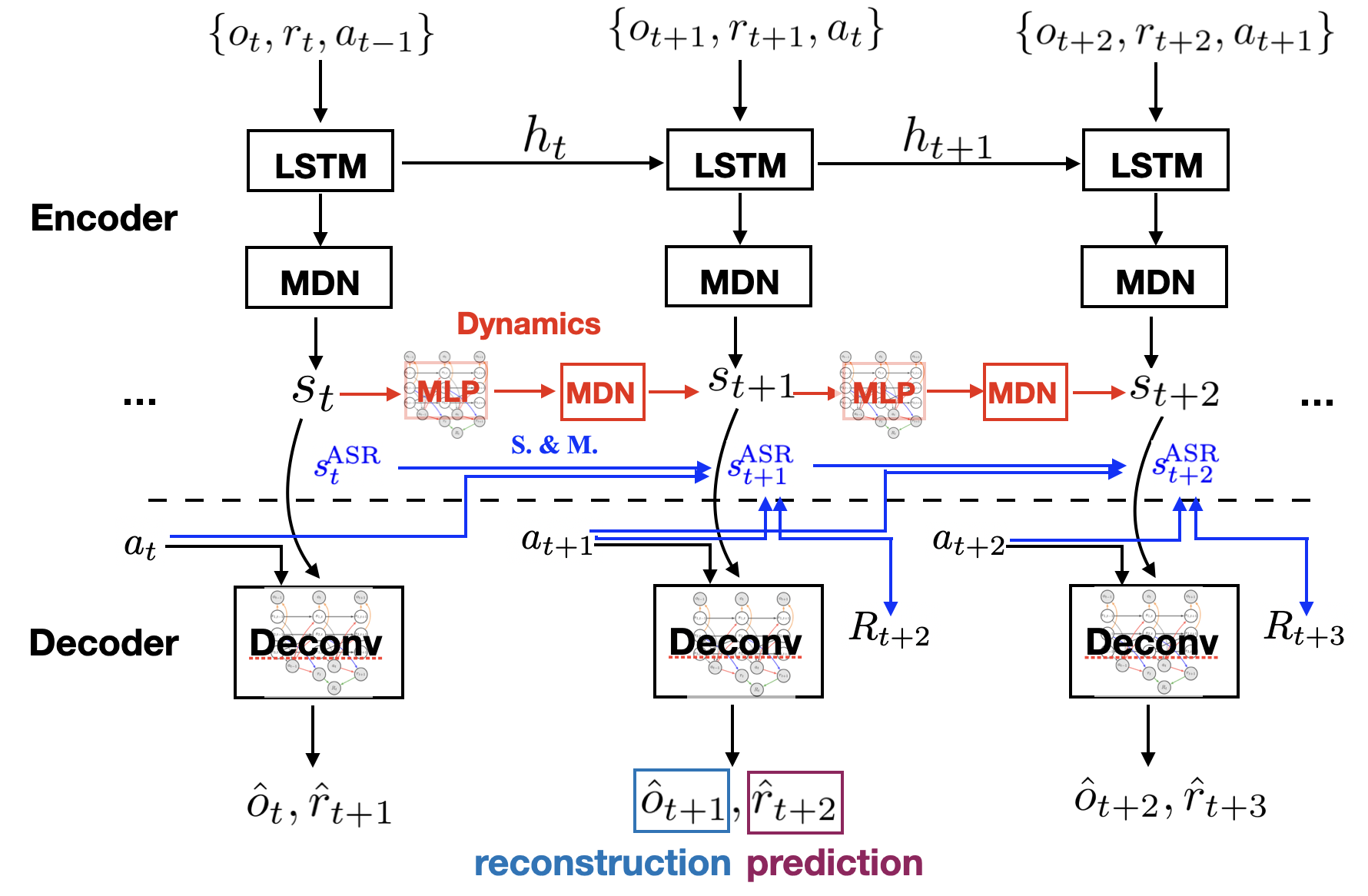
Figure 3: Diagram of neural network architecture to learn state representations. The corresponding structural constraints are involved in “Deconv” and “MLP”, and “S.&M." represents the regularization part for minimal sufficient state representation learning.

Below are the details of each component in the above objective function:

• Reconstruction and prediction components: These two parts are commonly used in sequential VAE. They aim to minimize the reconstruction error and prediction error of the perceived signal $o_{t}$ and the reward $r_{t}$.

• Transition component: To achieve the property that state representations satisfy an MDP, we explicitly model the transition dynamics: $\log p_{\gamma}(\tilde{\vec{s}}_{t}|\tilde{\vec{s}}_{t-1},a_{t-1};D_{\vec{s}},D_{a{\hbox{\rule[0.0pt]{0.0pt}{0.0pt}}\mkern-4.0mu\hbox{\char 41\relax}}\vec{s}})$. In particular, $\tilde{\vec{s}}_{t}|\tilde{\vec{s}}_{t-1}$ is modelled with a mixture of Gaussians: $\sum_{k=1}^{K}\!\pi_{k}\mathcal{N}\big{(}\boldsymbol{\mu}_{k}(\tilde{\vec{s}}_{t-1},\!a_{t-1}),\Sigma_{k}(\tilde{\vec{s}}_{t-1},\!a_{t-1})\big{)}$, where $K$ is the number of mixtures, $\boldsymbol{\mu}_{k}(\cdot)$ and $\Sigma_{k}(\cdot)$ are given by multi-layer perceptrons (MLP) with inputs $\tilde{\vec{s}}_{t-1}$ and $a_{t-1}$, parameters $\gamma$, and structural constraints ${D_{\vec{s}}}$ and ${D_{a{\hbox{\rule[0.0pt]{0.0pt}{0.0pt}}\mkern-4.0mu\hbox{\char 41\relax}}\vec{s}}}$. This explicit constraint on state dynamics is essential for establishing a Markov chain in latent space and for learning a representation for long-term predictions. Note that unlike in traditional VAE (Kingma & Welling, 2013), we do not assume that different dimensions in $\tilde{\vec{s}}_{t}$ are marginally independent, but model their structural relationships explicitly to achieve conditional independence.

• KL-divergence constraint: The KL divergence is used to constrain the state space with multiple purposes: (1) It is used in the lower bound of $\log P(\mathbf{y}_{1:T})$ to achieve conditional disentanglement between $q_{\phi}(\tilde{s}_{i,t}|\cdot)$ and $q_{\phi}(\tilde{s}_{j,t}|\cdot)$ for $i\neq j$, (2) and also to achieve further restrictions of minimality of ASRs.

• Sufficiency & minimality constraints: We achieve minimal sufficient state representations for the downstream policy learning by leveraging the conditional mutual information between $\tilde{\vec{s}}_{t}^{\,\text{ASR}}$ and $R_{t+1}$, and structural constraints. For details, please refer to Section 2.1.

• Sparsity constraints: According to the edge-minimality property (Zhang & Spirtes, 2011), we additionally put sparsity constraints on structural matrices to achieve better identifiability. In particular, we use $L_{1}$ norm of the structural matrices as regularizers in the objective function to achieve sparsity of the solution.

Figure 3 gives the diagram of the neural network architecture in model training. We use SS-VAE to learn the environment model and ASRs. Specifically, the encoder, which is used to learn the inference model $q_{\phi}(\tilde{\vec{s}}_{t}|\tilde{\vec{s}}_{t-1},\mathbf{y}_{1:t},a_{1:t-1})$, includes a Long Short-Term Memory (LSTM (Hochreiter & Schmidhuber, 1997)) to encode the sequential information with output $h_{t}$ and a Mixture Density Network (MDN (Bishop, 1994)) to output the parameters of MoGs. At each time instance, the input $\langle o_{t+1},r_{t+1},a_{t}\rangle$ is projected to the encoder and a sample of $\tilde{\vec{s}}_{t+1}$ is inferred from $q_{\phi}$ as output. The generated sample further acts as an input to the decoder, together with $a_{t+1}$ and structural matrices $D_{\vec{s}{\hbox{\rule[0.0pt]{0.0pt}{0.0pt}}\mkern-4.0mu\hbox{\char 41\relax}}o},D_{\vec{s}{\hbox{\rule[0.0pt]{0.0pt}{0.0pt}}\mkern-4.0mu\hbox{\char 41\relax}}r}$, and $D_{a{\hbox{\rule[0.0pt]{0.0pt}{0.0pt}}\mkern-4.0mu\hbox{\char 41\relax}}r}$. Then the decoder outputs $\hat{o}_{t+1}$ and $\hat{r}_{t+2}$. Moreover, the state dynamics which satisfies a Markov process and is embedded with structural constraints $D_{\vec{s}}$ and $D_{a{\hbox{\rule[0.0pt]{0.0pt}{0.0pt}}\mkern-4.0mu\hbox{\char 41\relax}}\vec{s}}$, is modeled with an MLP and MDN, marked with red in Figure 3. The part for minimal sufficient representations (denoted by S.&M.) uses MLP and is marked with blue. During training, we approximate the expectation in $\mathcal{L}$ by sampling and then jointly learn all parameters by maximizing $\mathcal{L}$ using stochastic gradient descent.

4 Policy Learning with ASRs

After estimating the generative environment model, we are ready to learn the optimal policy, where the policy function only depends on low-dimensional ASRs, instead of high-dimensional images. The entire procedure roughly contains the following three parts: (1) data collection with a random or sub-optimal policy, (2) environment model estimation (with details in Section 3), and (3) policy learning with ASRs. Notably, the generative environment model is fixed, regardless of the behavior policy that is used to generate the data, and after learning the environment model, as well as the inference model for ASRs, our framework is flexible for both model-free and model-based policy learning.

Model-Free Policy Learning.

For model-free policy learning, we make use of the learned environment model to infer ASRs $\tilde{\vec{s}}_{t}^{\,\text{ASR}}$ from past observed sequences $\{o_{\leq t},r_{\leq t},a_{\leq t-1}\}$ and then predict the action with the estimated low-dimensional ASRs. Our method is flexible to use a wide range of model-free methods; for example, one may use deep Q-learning for discrete actions (Mnih et al., 2015) and deep deterministic policy gradient (DDPG) for continuous actions (Lillicrap et al., 2015). Algorithm 1 in Appendix G gives the detailed procedure of model-free policy learning with ASRs in partially observable environments.

Model-Based Policy Learning.

The downside of model-free RL algorithms is that they are usually data hungry, requiring very large amounts of interactions. On the contrary, model-based RL algorithms enjoy much better sample efficiency. Hence, we make use of the learned generative environment model, including the transition dynamics, observation function, and reward function, for model-based policy optimization. Based on the generative environment model, one can learn behaviors from imagined outcomes to increase sample-efficiency and mitigate heavy and possibly risky interactions with the environment. We present the procedure of the classic Dyna algorithm (Sutton, 1990; Sutton & Barto, 2018) with ASRs in Algorithm 2 in Appendix G.

5 Experiments

To evaluate the proposed approach, we conducted experiments on both CarRacing environment (Klimov, 2016) with an illustration in Figure 5 and VizDoom (Kempka et al., 2016) environment with an illustration in Figure 5, following the setup in the world model (Ha & Schmidhuber, 2018) for a fair comparison. It is known that CarRacing is very challenging—the recent world model (Ha & Schmidhuber, 2018) is the first known solution to achieve the score required to solve the task. Without stated otherwise, all results were averaged across five random seeds, with standard deviation shown in the shaded area.

5.1 CarRacing Experiment

CarRacing is a continuous control task with three continuous actions: steering left/right, acceleration, and brake. Reward is $-0.1$ every frame and $+1000/N$ for every track tile visited, where $N$ is the total number of tiles in track. It is obvious that the CarRacing environment is partially observable: by just looking at the current frame, although we can tell the position of the car, we know neither its direction nor velocity that are essential for controlling the car. For a fair comparison, we followed a similar setting as in Ha & Schmidhuber (2018). Specifically, we collected a dataset of $10k$ random rollouts of the environment, and each runs with a random policy until failure. The dimensionality of latent states $\tilde{\vec{s}}_{t}$ was set to $\tilde{d}=32$, determined by hyperparameter tuning.

Figure 4: An illustration of Car Racing environment.

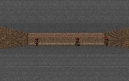
Figure 5: An illustration of VizDoom take cover scenario.

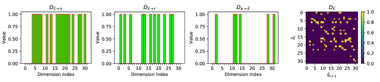
Figure 6: Visualization of estimated structural matrices $D_{\vec{s}{\hbox{\rule[0.0pt]{0.0pt}{0.0pt}}\mkern-4.0mu\hbox{\char 41\relax}}o}$, $D_{\vec{s}{\hbox{\rule[0.0pt]{0.0pt}{0.0pt}}\mkern-4.0mu\hbox{\char 41\relax}}r}$, $D_{a{\hbox{\rule[0.0pt]{0.0pt}{0.0pt}}\mkern-4.0mu\hbox{\char 41\relax}}\vec{s}}$, and $D_{\vec{s}}$ in Car Racing.

Analysis of ASRs.

To demonstrate the structures over observed frames, latent states, actions, and rewards, we visualized the learned $D_{\vec{s}{\hbox{\rule[0.0pt]{0.0pt}{0.0pt}}\mkern-4.0mu\hbox{\char 41\relax}}o}$, $D_{\vec{s}{\hbox{\rule[0.0pt]{0.0pt}{0.0pt}}\mkern-4.0mu\hbox{\char 41\relax}}r}$, $D_{\vec{s}}$, and $D_{a{\hbox{\rule[0.0pt]{0.0pt}{0.0pt}}\mkern-4.0mu\hbox{\char 41\relax}}\vec{s}}$, as shown in Figure 6. Intuitively, we can see that $D_{\vec{s}{\hbox{\rule[0.0pt]{0.0pt}{0.0pt}}\mkern-4.0mu\hbox{\char 41\relax}}r}$ and $D_{a{\hbox{\rule[0.0pt]{0.0pt}{0.0pt}}\mkern-4.0mu\hbox{\char 41\relax}}\vec{s}}$ have many values close to zero, meaning that the reward is only influenced by a small number of state dimensions, and not many state dimensions are influenced by the action. Furthermore, from $D_{\vec{s}}$, we found that there are influences from $\tilde{\vec{s}}_{i,t}$ to $\tilde{\vec{s}}_{i,t+1}$ (diagonal values) for most state dimensions, which is reasonable because we want to learn an MDP over the underlying states, while the connections across states (off-diagonal values) are much sparser. Compared to the original 32-dim latent states, ASRs have only 21 dimensions. Below, we empirically showed that the low-dimensional ASRs significantly improve the policy learning performance in terms of both efficiency and efficacy.

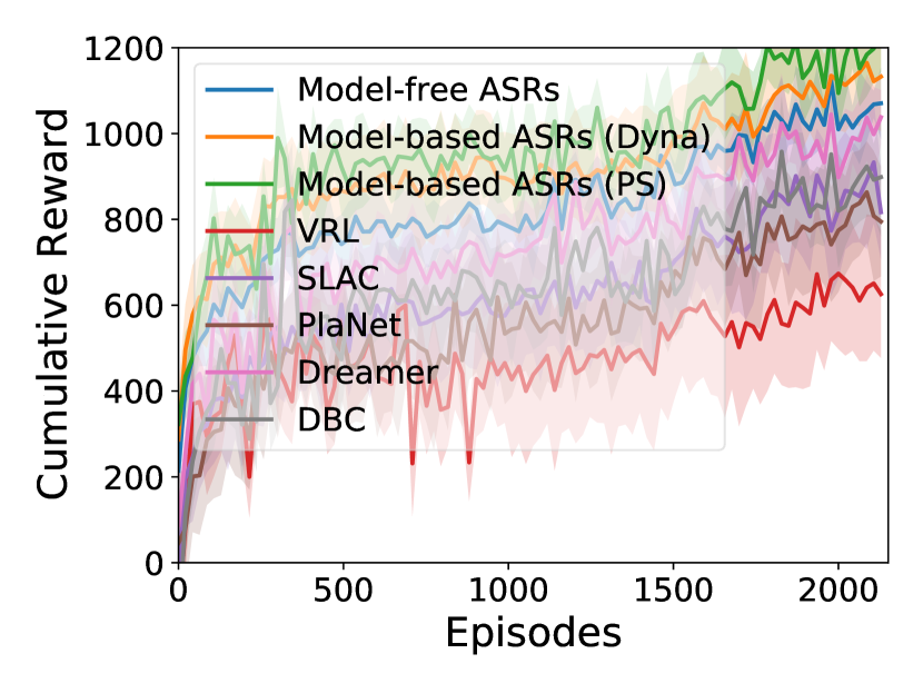
Figure 7: Cumulative rewards of model-based ASRs, model-free ASRs, VRL, SLAC, PlaNet, DBC and Dreamer evaluated on CarRacing.

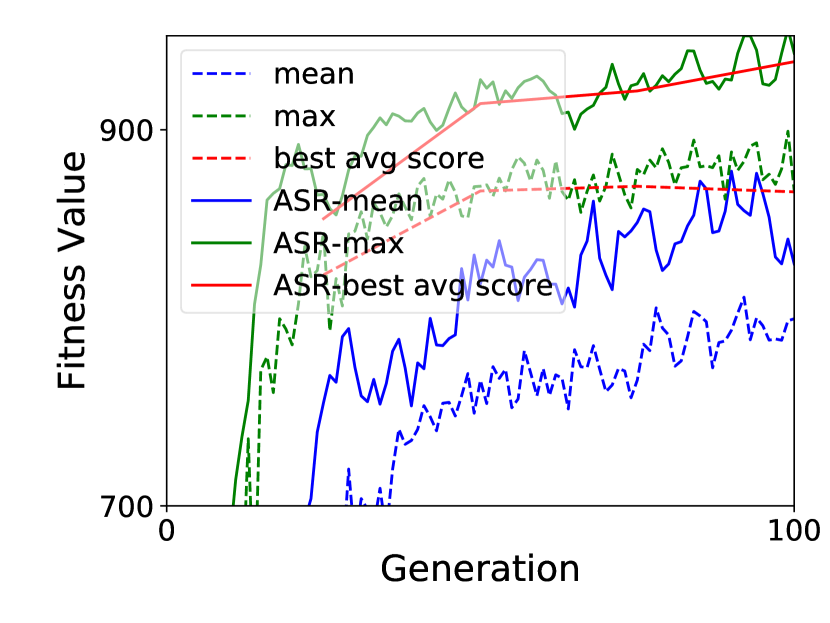
Figure 8: Fitness Value of ASRs compared to world models evaluated on CarRacing, including mean score, max score, and the best average score.

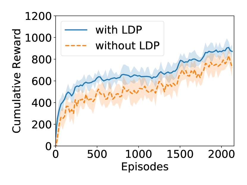
Figure 9: Ablation study of latent dynamics prediction (LDP) evaluated on Car Racing with model-free ASR.

Comparison Between Model-Free and Model-Based ASRs.

We applied both model-free (DDPG) (Lillicrap et al., 2015) and model-based (Dyna and Prioritized Sweeping) algorithms (Sutton, 1990) to ASRs (with 21-dims). As shown in Figure 9, interestingly, by taking advantage of the learned generative model, model-based ASRs is superior to model-free ASRs at a faster rate, which demonstrates the effectiveness of the learned model. It also shows that with the estimated environment model and ASRs, we can learn behaviors from imagined outcomes to improve sample-efficiency.

Comparison with VRL, SLAC, PlaNet, DBC, and Dreamer.

We also compared the proposed framework of policy learning with ASRs (with 21-dims) with 1) the same learning strategy but with vanilla representation learning (VRL, implemented without the components for minimal sufficient state representations as in Eq. (5)), 2) SLAC (Lee et al., 2019), 3) PlaNet (Hafner et al., 2018), 4) DBC (Zhang et al., 2021), and 5) Dreamer (Hafner et al., 2019). For a fair comparison, the latent dimensions of VRL, PlaNet, SLAC, DBC and Dreamer are set to 21 as well, and we require all of them to have the model capacity similar to ours (i.e., similar model architectures). From Figure 9, we can see that our methods, both model-free and model-based, obviously outperform others. It is worth noting that the huge performance difference between ASRs and VRL shows that the components for minimal sufficient state representations play a pivotal role in our objective.

Comparison with World Models.

In light of the fact that world models (Ha & Schmidhuber, 2018) achieved good performance in CarRacing, we further compared our method (with 21-dim ASRs) with the world model. For a fair comparison, following Ha & Schmidhuber (2018), we also used the Covariance-Matrix Adaptation Evolution Strategy (CMA-ES) (Hansen, 2016) with a population of 64 agents to optimize the parameters of the controller. In addition, following a similar setting as in Ha & Schmidhuber (2018) (where the agent’s fitness value is defined as the average cumulative reward of the 16 random rollouts), we show the fitness values of the best performer (max) and the population (mean) at each generation (Figure 9). We also took the best performing agent at the end of every 25 generations and tested it over 1024 random rollout scenarios to record the average (best avg score). It is obvious that our method (denoted by ASR-*) has a more efficient and also efficacy training process. The best average score of ASRs is 65 higher than that of world models.

Comparison with Dreamer and DBC with Background Distraction.

We further compared ASRs (with 21-dims) with Dreamer and DBC when there are natural video distractors in CarRacing; we chose Dreamer and DBC, because their performance are relatively better than other comparisons when there are no distractors. Specifically, we followed Zhang et al. (2021) to incorporate natural video from the Kinetics dataset (Kay et al., 2017) as background in CarRacing. Similarly, for a fair comparison, we require all of them to have the same latent dimensions and have the similar model capacity. As shown in Table 12, we can see that our method outperforms both Dreamer and DBC.

Ablation Study.

We further performed ablation studies on latent dynamics prediction; that is, we compared with the case when the transition dynamics in Fig. 2 is not explicitly modeled, but is replaced with a standard normal distribution. Figure 9 shows that by explicitly modelling the transition dynamics (denoted by with LDP), the cumulative reward has an obvious improvement over the one without modelling the transition dynamics (denoted by without LDP).

Model Cumulative Rewards Dreamer $621\pm 124.5$ DBC $803\pm 112.5$ Model-free ASRs $938\pm 87.2$ Model-based ASRs $954\pm 98.6$

Figure 10: Comparisons with Dreamer and DBC in CarRacing with natural video distractors, after 2000 training episodes, with standard error.

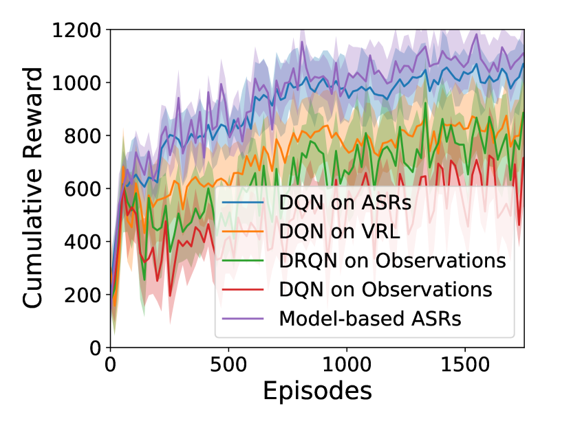
Figure 11: Comparing ASRs and SOTA methods evaluated on VizDoom.

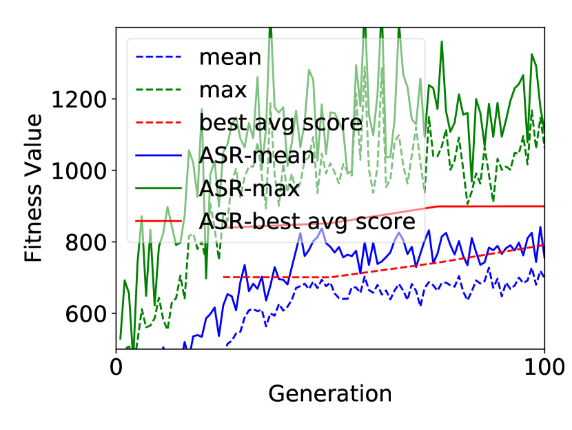
Figure 12: Fitness value of ASRs (with CMA-ES) compared to world models evaluated on VizDoom.

5.2 VizDoom Experiment

We also applied the proposed method to VizDoom take cover scenario (Kempka et al., 2016), which is a discrete control problem with two actions: move left and move right. Reward is +1 at each time step while alive, and the cumulative reward is defined to be the number of time steps the agent manages to stay alive during an episode.

Considering that in the take over scenario the action space is discrete, we applied the widely used DQN (Mnih et al., 2013) on ASRs for policy learning. In addition to the comparisons with VRL (as in CarRacing) and DQN on raw observations, we further compared with another common approach to POMDPs: DRQN (Hausknecht & Stone, 2015). As shown in Figure 12, DQN on ASRs achieve a much better performance than all other comparisons, and in particular, DQN on ASRs outperforms DRQN on observations by around 400 on average in terms of cumulative reward. Similarly, we applied model-based (Dyna) algorithms (Sutton, 1990) to ASRs (with 21-dims). As shown in Figure 12, we can draw the same conclusion that by taking advantage of the learned generative model, model-based ASRs is superior to model-free ASRs at a faster rate. We also applied ASRs to world models, where Figure 12 shows that our method with ASRs (denoted by ASR-*) achieves a better performance.

6 Related Work

In the past few years, a number of approaches have been proposed to learn low-dimensional Markovian representations, which capture the variation in the environment generated by the agent’s actions, without direct supervision (Lesort et al., 2018; Krishnan et al., 2015; Karl et al., 2016; Ha & Schmidhuber, 2018; Watter et al., 2015; Zhang et al., 2018; Kulkarni et al., 2016; Mahadevan & Maggioni, 2007; Gelada et al., 2019; Gregor et al., 2018; Ghosh et al., 2019; Zhang et al., 2021). Common strategies for such state representation learning include reconstructing the observation, learning a forward model, or learning an inverse model. Furthermore, prior knowledge, such as temporal continuity (Wiskott & Sejnowski, 2002), can be added to constrain the state space.

Recently, much attention has been paid to world models, which try to learn an abstract representation of both spatial and temporal aspects of the high-dimensional input sequences (Watter et al., 2015; Ebert et al., 2017; Ha & Schmidhuber, 2018; Hafner et al., 2018; Zhang et al., 2019b; Gelada et al., 2019; Kaiser et al., 2019; Hafner et al., 2019, 2020). Based on the learned world model, agents can perform model-based RL or planning. Our proposed method is also in the class of world models, which models the generative environment model, and additionally, encodes structural constraints and achieves the sufficiency and minimality of the estimated state representations from the view of generative and selection process. In contrast, Shu et al. (2020) makes use of contrastive loss, as an alternative of reconstruction loss; however, it only focuses on the transition dynamics and also fails to ensure the sufficiency and minimality. Another line of approaches of state representation learning is based on predictive state representations (PSRs) (Littman & Sutton, 2002; Singh et al., 2004). A recent approach generalizes PSRs to nonlinear predictive models, by exploiting the coarsest partition of histories into classes that are maximally predictive of the future (Zhang et al., 2019a). Moreover, bisimulation-based methods have also attracted much attention (Castro, 2020; Zhang et al., 2021).

On the other hand, our work is also related to Bayesian network learning and causal discovery (Spirtes et al., 1993; Pearl, 2000; Huang* et al., 2020). For example, Strehl et al. (2007) considers factorized-state MDP with structures being modeled with dynamic Bayesian network or decision trees. Incorporating such structure information has shown benefits in several machine learning tasks (Zhang* et al., 2020; Huang et al., 2019), and in this paper, we show its advantages in POMDPs.

7 Conclusions and Future Work

In this paper, we develop a principled framework to characterize a minimal set of state representations that suffice for policy learning, by making use of structural constraints and the goal of maximizing cumulative reward in policy learning. Accordingly, we propose SS-VAE to reliably extract such a set of state representations from raw observations. The estimated environment model and ASRs allow learning behaviors from imagined outcomes in the compact latent space, which effectively reduce sample complexity and possibly risky interactions with the environment. The proposed approach shows promising results on complex environments–CarRacing and Vizdoom. The future work along this direction include investigating identifiability conditions in general nonlinear cases and extending the approach to cover heterogeneous environments, where the generating processes may change over time or across domains.

Appendices for “Action-Sufficient State Representation Learning for Control with Structural Constraints"

Appendix A Proof of Proposition 1

We first give the definitions of the Markov condition and the faithfulness assumption, which will be used in the proof.

Definition 2 (Global Markov Condition (Spirtes et al., 1993; Pearl, 2000)).

The distribution $p$ over a set of variables $\mathbf{V}$ satisfies the global Markov property on graph $G$ if for any partition $(A,B,C)$ such that if $B$ d-separates $A$ from $C$, then $p(A,C|B)=p(A|B)p(C|B)$.

Definition 3 (Faithfulness Assumption (Spirtes et al., 1993; Pearl, 2000)).

There are no independencies between variables that are not entailed by the Markov Condition.

Below, we give the proof of Proposition 1.

Proof.

The proof contains the following three steps.

• In step 1, we show that a state dimension $s_{i,t}$ is in ASRs, that is, it has a directed path to $r_{t+\tau}$ and the path does not go through any action variable (which is equivalent to the recursive definition of ASR), if and only if $s_{i,t}\not\!\perp\!\!\!\perp R_{t+1}|a_{t-1:t},\vec{s}_{t-1}$.

• In step 2, we show that for $s_{i,t}$ with $s_{i,t}\not\!\perp\!\!\!\perp R_{t+1}|a_{t-1:t},\vec{s}_{t-1}$, if and only if $s_{i,t}\not\!\perp\!\!\!\perp R_{t+1}|a_{t-1:t},\vec{s}_{t-1}^{\text{ASR}}$.

• In step 3, we show that ASRs $\vec{s}_{t}^{\text{ASR}}$ are minimal sufficient for policy learning.

Step 1:

We first show that if a state dimension $s_{i,t}$ is in ASRs, then $s_{i,t}\not\!\perp\!\!\!\perp R_{t+1}|a_{t-1:t},\vec{s}_{t-1}$.

We prove it by contradiction. Suppose that $s_{i,t}$ is independent of $R_{t+1}$ given $a_{t-1:t}$ and $\vec{s}_{t-1}$. Then according to the faithfulness assumption, we can see from the graph that $s_{i,t}$ does not have a directed path to $r_{t+\tau}$, which contradicts to the assumption, because, otherwise, $a_{t-1:t}$ and $\vec{s}_{t-1}$ cannot break the paths between $s_{i,t}$ and $R_{t+1}$ which leads to the dependence.

We next show that if $s_{i,t}\not\!\perp\!\!\!\perp R_{t+1}|a_{t-1:t},\vec{s}_{t-1}$, then $s_{i,t}\in\vec{s}_{t}^{\,\text{ASR}}$.

Similarly, by contradiction suppose that $s_{i,t}$ does not have a directed path to $r_{t+\tau}$. From the graph, it is easy to see that $a_{t-1:t}$ and $\vec{s}_{t-1}$ must break the path between $s_{i,t}$ and $R_{t+1}$. According to the Markov assumption, $s_{i,t}$ is independent of $R_{t+1}$ given $a_{t-1:t}$ and $\vec{s}_{t-1}$, which contradicts to the assumption. Since we have a contradiction, it must be that $s_{i,t}$ has a directed path to $r_{t+\tau}$.

Step 2:

In step 1, we have shown that $s_{i,t}\not\!\perp\!\!\!\perp R_{t+1}|a_{t-1:t},\vec{s}_{t-1}$, if and only if it has a directed path to $r_{t+\tau}$. From the graph, it is easy to see that for those state dimensions which have a directed path to $r_{t+\tau}$, $a_{t-1:t}$ and $\vec{s}_{t-1}^{\text{ASR}}$ cannot break the path between $s_{i,t}$ and $R_{t+1}$. Moreover, for those state dimensions which do not have a directed path to $r_{t+\tau}$, $a_{t-1:t}$ and $\vec{s}_{t-1}^{\text{ASR}}$ are enough to break the path between $s_{i,t}$ and $R_{t+1}$.

Therefore, for $s_{i,t}$ with $s_{i,t}\not\!\perp\!\!\!\perp R_{t+1}|a_{t-1:t},\vec{s}_{t-1}$, if and only if $s_{i,t}\not\!\perp\!\!\!\perp R_{t+1}|a_{t-1:t},\vec{s}_{t-1}^{\text{ASR}}$.

Step 3:

In the previous steps, it has been shown that if a state dimension $s_{i,t}$ is in ASRs, then $s_{i,t}\not\!\perp\!\!\!\perp R_{t+1}|a_{t-1:t},\vec{s}_{t-1}^{\text{ASR}}$, and if a state dimension $s_{i,t}$ is not in ASRs, then $s_{i,t}\mathchoice{\mathrel{\hbox to0.0pt{$\displaystyle\perp$\hss}\mkern 2.0mu{\displaystyle\perp}}}{\mathrel{\hbox to0.0pt{$\textstyle\perp$\hss}\mkern 2.0mu{\textstyle\perp}}}{\mathrel{\hbox to0.0pt{$\scriptstyle\perp$\hss}\mkern 2.0mu{\scriptstyle\perp}}}{\mathrel{\hbox to0.0pt{$\scriptscriptstyle\perp$\hss}\mkern 2.0mu{\scriptscriptstyle\perp}}}R_{t+1}|a_{t-1:t},\vec{s}_{t-1}^{\text{ASR}}$. This implies that $\vec{s}_{t}^{\text{ASR}}$ are minimal sufficient for policy learning to maximize the future reward.

∎

Appendix B Learning the ASRs under a Random Policy

When collecting the data, that are used to learn the environment model and ASRs, with random actions, it is apparent to observe that actions $a_{t}$ and ASRs $\vec{s}_{t}^{\,\text{ASR}}$ are dependent only conditioning on the cumulative reward and previous state—this is a type of dependence relationship induced by selection on the effect (reward). We can then learn the ASRs by maximizing

$$I(\tilde{\vec{s}}_{t}^{\,\text{ASR}};a_{t}\,|\,R_{t+1},\tilde{\vec{s}}_{t-1}^{\,\text{ASR}})-I(\tilde{\vec{s}}_{t}^{\,\text{C}};a_{t}\,|\,R_{t+1},\tilde{\vec{s}}_{t-1}^{\,\text{ASR}}),$$ (7)

where $\tilde{\vec{s}}^{\,\text{C}}=\tilde{\vec{s}}\backslash\tilde{\vec{s}}^{\,\text{ASR}}$, and $I$ denotes mutual information. Since $I(\tilde{\vec{s}}_{t}^{\,\text{ASR}};a_{t}\,|\,R_{t+1},\tilde{\vec{s}}_{t-1}^{\,\text{ASR}})=H(a_{t}\,|\,R_{t+1},\tilde{\vec{s}}_{t-1}^{\,\text{ASR}})-H(a_{t}\,|\,\tilde{\vec{s}}_{t-1:t}^{\,\text{ASR}},R_{t+1})$, where $H(\cdot)$ denotes the conditional entropy, we can estimate ASRs by maximizing $H(a_{t}\,|\,R_{t+1},\tilde{\vec{s}}_{t-1}^{\,\text{ASR}})-H(a_{t}\,|\,\tilde{\vec{s}}_{t-1:t}^{\,\text{ASR}},R_{t+1})$, with

$$H(a_{t}|\tilde{\vec{s}}_{t-1:t}^{\text{ASR}},R_{t+1})=-\mathbb{E}_{q_{\phi,\alpha_{1}}}\big{\{}\log p_{\alpha_{1}}(a_{t}|\tilde{\vec{s}}_{t-1:t}^{\,\text{ASR}}\,,R_{t+1})\big{\}}=-\mathbb{E}_{q_{\phi,\alpha_{1}}}\big{\{}\log p_{\alpha_{1}}(a_{t}|\tilde{D}^{ASR}\odot\tilde{\vec{s}}_{t-1:t},R_{t+1})\big{\}},$$

and

$$H(a_{t}|R_{t+1},\tilde{\vec{s}}_{t-1}^{\,\text{ASR}})=-\mathbb{E}_{q_{\phi,\alpha_{2}}}\big{\{}\log p_{\alpha_{2}}(a_{t}|R_{t+1},\tilde{\vec{s}}_{t-1}^{\,\text{ASR}})\big{\}},=-\mathbb{E}_{q_{\phi,\alpha_{2}}}\big{\{}\log p_{\alpha_{2}}(a_{t}|\tilde{D}^{ASR}\odot\tilde{\vec{s}}_{t-1}^{\,\text{ASR}},R_{t+1})\big{\}},$$

where $p_{\alpha_{i}}$, for $i=1,2$, denotes the probabilistic predictive model of $a_{t}$ with parameters $\alpha_{i}$, $q_{\phi\!,\alpha_{i}}$ is the joint distribution over $\tilde{\vec{s}}_{t}$ and $a_{t}$ with $q_{\phi\!,\alpha_{i}}=q_{\phi}p_{\alpha_{i}}$, and $q_{\phi}(\tilde{\vec{s}}_{t}|\tilde{\vec{s}}_{t-1},\mathbf{y}_{1:t},a_{1:t-1})$ is the probabilistic inference model of $\tilde{\vec{s}}_{t}$ with parameters $\phi$ and $\mathbf{y}_{t}\!=\!(o_{t}^{T},r_{t}^{T})$, and $\tilde{D}^{\,\text{ASR}}\in\{0,1\}^{\tilde{d}\times 1}$ is a binary vector indicating which dimensions of $\tilde{\vec{s}}_{t}$ are in $\tilde{\vec{s}}_{t}^{\,\text{ASR}}$, so $\tilde{D}^{\,\text{ASR}}\odot\tilde{\vec{s}}_{t}$ gives ASRs $\tilde{\vec{s}}_{t}^{\,\text{ASR}}$. Similarly, we can also represent $I(\tilde{\vec{s}}_{t}^{\,\text{C}};a_{t}\,|\,R_{t+1},\tilde{\vec{s}}_{t-1}^{\,\text{ASR}})$ in the same way. Accordingly, the “sufficiency & Minimality” term in the objective function as shown in Figure 2 should be replaced by (7), and the corresponding diagram of neural network architecture is as shown in Figure 13.

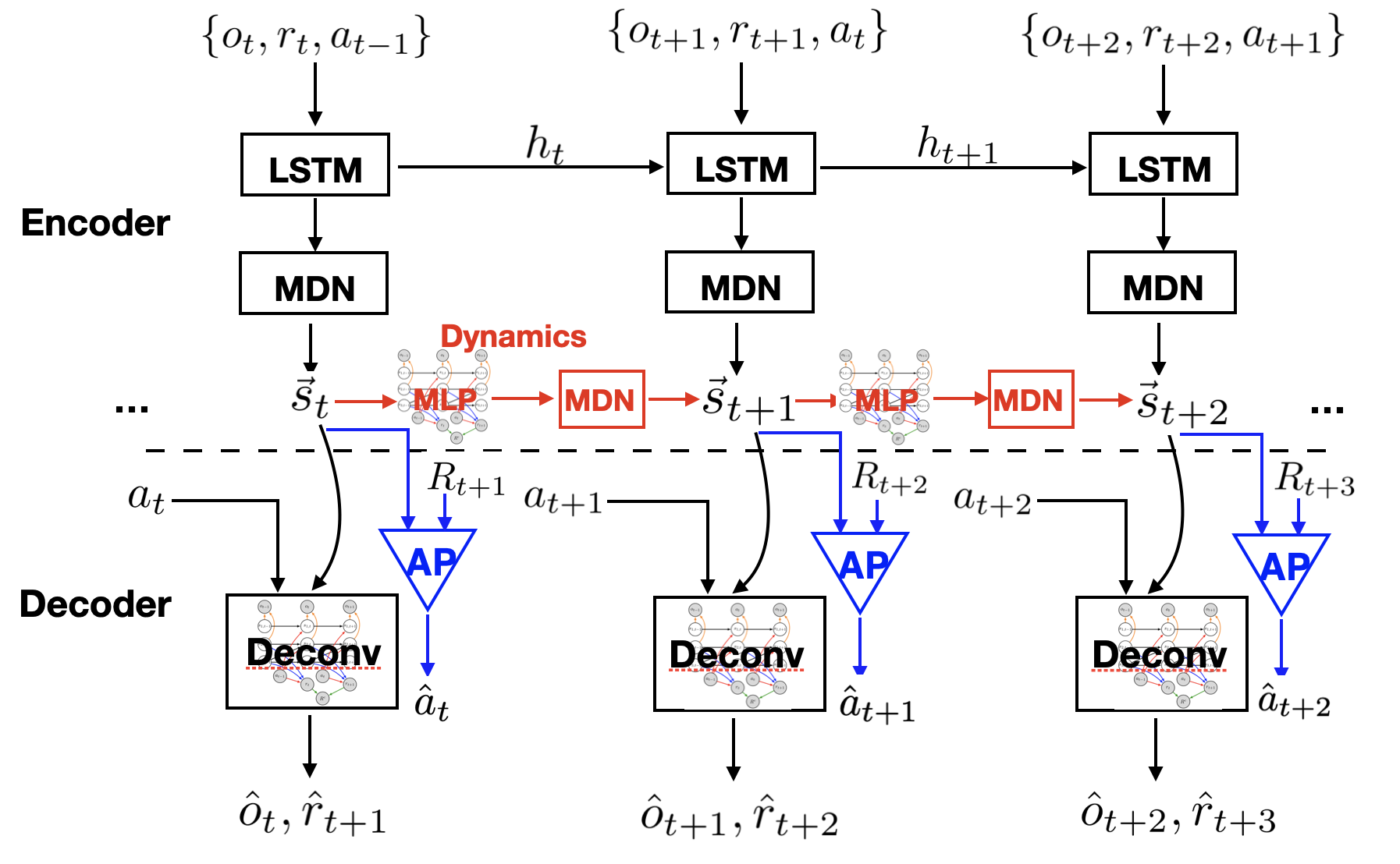
Figure 13: Diagram of neural network architecture to learn state representations. The corresponding structural constraints are involved in “Deconv” and “MLP”, and “AP" represents the action prediction part for sufficient state representation learning.

Appendix C Further Regularization of Minimality

In this section, we give the detailed derivation on the further regularization of minimality of state representations given in Section 2.1, which is similar to that in the information bottleneck. We achieve it by minimizing conditional mutual information between observed high-dimensional signals $\mathbf{y}_{t}$, where $\mathbf{y}_{t}=\{o_{t}^{T},r_{t}^{T}\}$, and the ASR $\tilde{\vec{s}}_{t}^{\,\text{ASR}}$ at time $t$ given data at previous time instances, and meanwhile minimizing the dimensionality of ASRs with sparsity constraints:

$$\lambda_{1}\sum\nolimits_{t=2}^{T}I(\mathbf{y}_{t};\tilde{\vec{s}}_{t}^{\,\text{ASR}}|\mathbf{y}_{1:t-1},a_{1:t-1},\tilde{\vec{s}}_{t-1})+\lambda_{2}\|\tilde{D}^{\,\text{ASR}}\|_{1}.$$

Note that in the above conditional mutual information, we need to conditional on the previous states $\tilde{\vec{s}}_{t-1}$, instead of $\tilde{\vec{s}}_{t-1}^{\,\text{ASR}}$, which two give different conditional mutual information. It can be shown by contradiction. Suppose $I(\mathbf{y}_{t};\tilde{\vec{s}}_{t}^{\,\text{ASR}}|\mathbf{y}_{1:t-1},a_{1:t-1},\tilde{\vec{s}}_{t-1})=I(\mathbf{y}_{t};\tilde{\vec{s}}_{t}^{\,\text{ASR}}|\mathbf{y}_{1:t-1},a_{1:t-1},\tilde{\vec{s}}_{t-1}^{\,\text{ASR}})$, and denote $\tilde{\vec{s}}^{\,C}=\tilde{\vec{s}}\backslash\tilde{\vec{s}}^{\,\text{ASR}}$. Then the equivalence implies that $\tilde{\vec{s}}_{t-1}^{\,C}$ is independent of $o_{t}$ (where $o_{t}\in\mathbf{y}_{t}$) given $\{\mathbf{y}_{1:t-1},a_{1:t-1},\tilde{\vec{s}}_{t-1}^{\,\text{ASR}}\}$. It is obviously violated for the example given in Figure 1, where $\tilde{\vec{s}}^{\,C}=s_{1}$ and $\tilde{\vec{s}}^{\,\text{ASR}}=\{s_{2},s_{3}\}$, and $s_{1,t-1}$ is dependent on $o_{t}$ given $\{\mathbf{y}_{1:t-1},a_{1:t-1},s_{2,{t-1}},s_{3,{t-1}}\}$. Hence, conditioning on $\tilde{\vec{s}}_{t-1}$ and $\tilde{\vec{s}}_{t-1}^{\,\text{ASR}}$ give different conditional mutual information. Therefore, in the above conditional mutual information, we need to condition on the previous states $\tilde{\vec{s}}_{t-1}$.

Moreover, the conditional mutual information $I(\mathbf{y}_{t};\tilde{\vec{s}}_{t}^{\,\text{ASR}}|\mathbf{y}_{1:t-1},a_{1:t-1},\tilde{\vec{s}}_{t-1})$ can be upper bound by a KL-divergence, and below we denote $\{\mathbf{y}_{1:t-1},a_{1:t-1},\tilde{\vec{s}}_{t-1}\}$ by $\mathbf{z_{t}}$:

$$\begin{array}[]{lll}I(\mathbf{y}_{t};\tilde{\vec{s}}_{t}^{\,\text{ASR}}|\mathbf{y}_{1:t-1},a_{1:t-1},\tilde{\vec{s}}_{t-1})\\ \equiv I(\mathbf{y}_{t};\tilde{\vec{s}}_{t}^{\,\text{ASR}}|\mathbf{z}_{t})\\ \equiv\mathbb{E}_{p(\mathbf{y}_{t},\tilde{\vec{s}}_{t}^{\,\text{ASR}},\mathbf{z}_{t})}\big{\{}\log\frac{q_{\phi}(\tilde{\vec{s}}_{t}^{\,\text{ASR}}|\mathbf{y}_{t},\mathbf{z}_{t})}{p(\tilde{\vec{s}}_{t}^{\,\text{ASR}}|\mathbf{z}_{t})}\big{\}}\\ =\mathbb{E}_{p(\mathbf{y}_{t},\tilde{\vec{s}}_{t}^{\,\text{ASR}},\mathbf{z}_{t})}\big{\{}\log\frac{q_{\phi}(\tilde{\vec{s}}_{t}^{\,\text{ASR}}|\mathbf{y}_{t},\mathbf{z}_{t})p_{\gamma}(\tilde{\vec{s}}_{t}^{\,\text{ASR}}|\tilde{\vec{s}}_{t-1},a_{t-1})}{p(\tilde{\vec{s}}_{t}^{\,\text{ASR}}|\mathbf{z}_{t})p_{\gamma}(\tilde{\vec{s}}_{t}^{\,\text{ASR}}|\tilde{\vec{s}}_{t-1},a_{t-1})}\big{\}}\\ =\mathbb{E}_{p(\mathbf{y}_{t},\tilde{\vec{s}}_{t}^{\,\text{ASR}},\mathbf{z}_{t})}\big{\{}\log\frac{q_{\phi}(\tilde{\vec{s}}_{t}^{\,\text{ASR}}|\mathbf{y}_{t},\mathbf{z}_{t})}{p_{\gamma}(\tilde{\vec{s}}_{t}^{\,\text{ASR}}|\tilde{\vec{s}}_{t-1},a_{t-1})}\big{\}}-\mathbb{E}_{p(\mathbf{z}_{t})}\big{\{}\text{KL}(p(\tilde{\vec{s}}_{t}^{\,\text{ASR}}|\mathbf{z}_{t})\|p_{\gamma}(\tilde{\vec{s}}_{t}^{\,\text{ASR}}|\tilde{\vec{s}}_{t-1},a_{t-1}))\big{\}}\\ \leq\mathbb{E}_{p(\mathbf{y}_{t},\mathbf{z}_{t})}\big{[}\text{KL}\big{(}q_{\phi}(\tilde{\vec{s}}_{t}^{\,\text{ASR}}|\mathbf{y}_{t},\mathbf{z}_{t})\|p_{\gamma}(\tilde{\vec{s}}_{t}^{\,\text{ASR}}|\tilde{\vec{s}}_{t-1},a_{t-1})\big{)}\big{]}\\ \equiv\mathbb{E}_{p(\tilde{\vec{s}}_{t-1},\mathbf{y}_{1:t},a_{1:t-1})}\big{[}\text{KL}\big{(}q_{\phi}(\tilde{\vec{s}}_{t}^{\,\text{ASR}}|\tilde{\vec{s}}_{t-1},\mathbf{y}_{1:t},a_{1:t-1})\|p_{\gamma}(\tilde{\vec{s}}_{t}^{\,\text{ASR}}|\tilde{\vec{s}}_{t-1},a_{t-1};D_{\vec{s}},D_{a{\hbox{\rule[0.0pt]{0.0pt}{0.0pt}}\mkern-4.0mu\hbox{\char 41\relax}}\vec{s}})\big{)}\big{]}\end{array}$$

with $p_{\gamma}$ being the transition dynamics of $\tilde{\vec{s}}_{t}$ with parameters $\gamma$.

Appendix D Assumptions of Proposition 2

To show the identifiability of the model in the linear case, we make the following assumptions:

1. $d_{o}+d_{r}\geq d_{s}$, where $|o_{t}|=d_{o}$, $|r_{t}|=d_{r}$, and $|s_{t}|=d_{s}$.

2. $(D_{\vec{s}{\hbox{\rule[0.0pt]{0.0pt}{0.0pt}}\mkern-4.0mu\hbox{\char 41\relax}}o}^{\top},D_{\vec{s}{\hbox{\rule[0.0pt]{0.0pt}{0.0pt}}\mkern-4.0mu\hbox{\char 41\relax}}r}^{\top})$ is full column rank and $D_{\vec{s}}$ is full rank.

3. The control signal $a_{t}$ is i.i.d. and the state $\vec{s}_{t}$ is stationary.

4. The process noise has a unit variance, i.e., $\text{var}(\eta_{t})=I$.

Appendix E Proof of Proposition 2

Proof.

The proof of the linear case without control signals has been shown in Zhang & Hyvärinen (2011). Below, we give the identifiability proof in the linear-Gaussian case with control signals:

$$\left\{\begin{array}[]{lll}o_{t}=D_{\vec{s}{\hbox{\rule[0.0pt]{0.0pt}{0.0pt}}\mkern-4.0mu\hbox{\char 41\relax}}o}^{\top}\vec{s}_{t}+e_{t},\\ r_{t+1}=D_{\vec{s}{\hbox{\rule[0.0pt]{0.0pt}{0.0pt}}\mkern-4.0mu\hbox{\char 41\relax}}r}^{\top}\vec{s}_{t}+D_{a{\hbox{\rule[0.0pt]{0.0pt}{0.0pt}}\mkern-4.0mu\hbox{\char 41\relax}}r}^{\top}a_{t}+\epsilon_{t+1},\\ \vec{s}_{t}=D_{\vec{s}}^{\top}\vec{s}_{t-1}+D_{a{\hbox{\rule[0.0pt]{0.0pt}{0.0pt}}\mkern-4.0mu\hbox{\char 41\relax}}\vec{s}}^{\top}a_{t-1}+\eta_{t}.\end{array}\right.$$ (8)

Let $\mathbf{y}_{t+1}=[o_{t}^{\top},r_{t+1}^{\top}]^{\top}$, $\ddot{D}_{\vec{s}{\hbox{\rule[0.0pt]{0.0pt}{0.0pt}}\mkern-4.0mu\hbox{\char 41\relax}}o}=[D_{\vec{s}{\hbox{\rule[0.0pt]{0.0pt}{0.0pt}}\mkern-4.0mu\hbox{\char 41\relax}}o}^{\top},D_{\vec{s}{\hbox{\rule[0.0pt]{0.0pt}{0.0pt}}\mkern-4.0mu\hbox{\char 41\relax}}r}^{\top}]^{\top}$, $\ddot{D}_{a{\hbox{\rule[0.0pt]{0.0pt}{0.0pt}}\mkern-4.0mu\hbox{\char 41\relax}}r}=[\vec{0}^{\top},D_{a{\hbox{\rule[0.0pt]{0.0pt}{0.0pt}}\mkern-4.0mu\hbox{\char 41\relax}}r}^{\top}]^{\top}$, and $\ddot{e}_{t}=[e_{t}^{\top},\epsilon_{t+1}^{\top}]^{\top}$. Then the above equation can be represented as:

$$\left\{\begin{array}[]{lll}\mathbf{y}_{t}=\ddot{D}_{\vec{s}{\hbox{\rule[0.0pt]{0.0pt}{0.0pt}}\mkern-4.0mu\hbox{\char 41\relax}}o}^{\top}\vec{s}_{t}+\ddot{D}_{a{\hbox{\rule[0.0pt]{0.0pt}{0.0pt}}\mkern-4.0mu\hbox{\char 41\relax}}r}^{\top}a_{t}+\ddot{e}_{t},\\ \vec{s}_{t}=D_{\vec{s}}^{\top}\vec{s}_{t-1}+D_{a{\hbox{\rule[0.0pt]{0.0pt}{0.0pt}}\mkern-4.0mu\hbox{\char 41\relax}}\vec{s}}^{\top}a_{t-1}+\eta_{t}.\end{array}\right.$$ (9)

Because the dynamic system is linear and Gaussian, we make use of the second-order statistics of the observed data to show the identifiability. We first consider the cross-covariance between $\mathbf{y}_{t+k}$ and $a_{t}$:

$$\left\{\begin{array}[]{lll}\text{Cov}(\mathbf{y}_{t+k},a_{t})=\ddot{D}_{\vec{s}{\hbox{\rule[0.0pt]{0.0pt}{0.0pt}}\mkern-4.0mu\hbox{\char 41\relax}}o}^{\top}D_{\vec{s}}^{k-1}D_{a{\hbox{\rule[0.0pt]{0.0pt}{0.0pt}}\mkern-4.0mu\hbox{\char 41\relax}}\vec{s}}^{\top}\cdot\text{Var}(a_{t}),&\text{if }k>0,\\ \text{Cov}(\mathbf{y}_{t+k},a_{t})=\ddot{D}_{a{\hbox{\rule[0.0pt]{0.0pt}{0.0pt}}\mkern-4.0mu\hbox{\char 41\relax}}r}^{\top}\cdot\text{Var}(a_{t}),&\text{if }k=0.\\ \end{array}\right.$$ (10)

Thus, from the cross-covariance between $\mathbf{y}_{t+k}$ and $a_{t}$, we can identify $\ddot{D}_{\vec{s}{\hbox{\rule[0.0pt]{0.0pt}{0.0pt}}\mkern-4.0mu\hbox{\char 41\relax}}o}^{\top}D_{a{\hbox{\rule[0.0pt]{0.0pt}{0.0pt}}\mkern-4.0mu\hbox{\char 41\relax}}\vec{s}}^{\top}$, $\ddot{D}_{a{\hbox{\rule[0.0pt]{0.0pt}{0.0pt}}\mkern-4.0mu\hbox{\char 41\relax}}r}$, and $\ddot{D}_{\vec{s}{\hbox{\rule[0.0pt]{0.0pt}{0.0pt}}\mkern-4.0mu\hbox{\char 41\relax}}o}^{\top}D_{\vec{s}}^{k}D_{a{\hbox{\rule[0.0pt]{0.0pt}{0.0pt}}\mkern-4.0mu\hbox{\char 41\relax}}\vec{s}}^{\top}$ for $k>0$.

Next, we consider the auto-covariance function of $\vec{s}$. Define the auto-covariance function of $\vec{s}$ at lag $k$ as $\mathbf{R}_{\vec{s}}(k)=\mathbb{E}[\vec{s}_{t}\vec{s}_{t+k}^{\top}]$, and similarly for $\mathbf{R}_{\mathbf{y}}(k)$. Clearly, $\mathbf{R}_{\vec{s}}(-k)=\mathbf{R}_{\vec{s}}(k)^{\top}$ and $\mathbf{R}_{\mathbf{y}}(-k)=\mathbf{R}_{\mathbf{y}}(k)^{\top}$. Then we have

$$\left\{\begin{array}[]{lll}\mathbf{R}_{\vec{s}}(k)=\mathbf{R}_{\vec{s}}(k-1)\cdot D_{\vec{s}},&\text{if }k>0,\\ \mathbf{R}_{\vec{s}}(k)=\mathbf{R}_{\vec{s}}^{\top}(1)\cdot D_{\vec{s}}+D_{a{\hbox{\rule[0.0pt]{0.0pt}{0.0pt}}\mkern-4.0mu\hbox{\char 41\relax}}\vec{s}}^{\top}\text{Var}(a_{t-1})D_{a{\hbox{\rule[0.0pt]{0.0pt}{0.0pt}}\mkern-4.0mu\hbox{\char 41\relax}}\vec{s}}+I,&\text{if }k=0.\end{array}\right.$$ (11)

Below, we first consider the case where $d_{o}+d_{r}=d_{s}$. Let $\tilde{\mathbf{y}}_{t}=\ddot{D}_{\vec{s}{\hbox{\rule[0.0pt]{0.0pt}{0.0pt}}\mkern-4.0mu\hbox{\char 41\relax}}o}^{\top}\vec{s}_{t}$, so ${\mathbf{y}}_{t}=\tilde{\mathbf{y}}_{t}+\ddot{D}_{a{\hbox{\rule[0.0pt]{0.0pt}{0.0pt}}\mkern-4.0mu\hbox{\char 41\relax}}r}^{\top}a_{t-1}+\ddot{e}_{t}$ and $\mathbf{R}_{\tilde{\mathbf{y}}}(k)=\ddot{D}_{\vec{s}{\hbox{\rule[0.0pt]{0.0pt}{0.0pt}}\mkern-4.0mu\hbox{\char 41\relax}}o}^{\top}\mathbf{R}_{\vec{s}_{t}}(k)\ddot{D}_{\vec{s}{\hbox{\rule[0.0pt]{0.0pt}{0.0pt}}\mkern-4.0mu\hbox{\char 41\relax}}o}$. $\mathbf{R}_{\tilde{\mathbf{y}}}(k)$ satisfies the recursive property:

$$\left\{\begin{array}[]{lll}\mathbf{R}_{\tilde{\mathbf{y}}}(k)=\mathbf{R}_{\tilde{\mathbf{y}}}(k-1)\cdot\Omega^{\top},&\text{if }k>0,\\ \mathbf{R}_{\tilde{\mathbf{y}}}(k)=\mathbf{R}_{\tilde{\mathbf{y}}}^{\top}(1)\cdot\Omega^{\top}+\ddot{D}_{\vec{s}{\hbox{\rule[0.0pt]{0.0pt}{0.0pt}}\mkern-4.0mu\hbox{\char 41\relax}}o}^{\top}(D_{a{\hbox{\rule[0.0pt]{0.0pt}{0.0pt}}\mkern-4.0mu\hbox{\char 41\relax}}\vec{s}}^{\top}\text{Var}(a_{t-1})D_{a{\hbox{\rule[0.0pt]{0.0pt}{0.0pt}}\mkern-4.0mu\hbox{\char 41\relax}}\vec{s}}+I)\ddot{D}_{\vec{s}{\hbox{\rule[0.0pt]{0.0pt}{0.0pt}}\mkern-4.0mu\hbox{\char 41\relax}}o},&\text{if }k=0,\end{array}\right.$$ (12)

where $\Omega=\ddot{D}_{\vec{s}{\hbox{\rule[0.0pt]{0.0pt}{0.0pt}}\mkern-4.0mu\hbox{\char 41\relax}}o}^{\top}D_{\vec{s}}\ddot{D}_{\vec{s}{\hbox{\rule[0.0pt]{0.0pt}{0.0pt}}\mkern-4.0mu\hbox{\char 41\relax}}o}^{-1}$.

Denote $S_{k}=\ddot{D}_{\vec{s}{\hbox{\rule[0.0pt]{0.0pt}{0.0pt}}\mkern-4.0mu\hbox{\char 41\relax}}o}^{\top}D_{\vec{s}}^{k-1}D_{a{\hbox{\rule[0.0pt]{0.0pt}{0.0pt}}\mkern-4.0mu\hbox{\char 41\relax}}\vec{s}}^{\top}\cdot\text{Var}(a_{t})$. Then we can derive the recursive property for $\mathbf{R}_{\mathbf{y}}(k)$:

$$\left\{\begin{array}[]{lll}\mathbf{R}_{\mathbf{y}}(k)=\mathbf{R}_{\mathbf{y}}(k-1)\cdot\Omega^{\top}-\ddot{D}_{a{\hbox{\rule[0.0pt]{0.0pt}{0.0pt}}\mkern-4.0mu\hbox{\char 41\relax}}r}^{\top}S_{k-1}^{\top}\Omega^{\top}+\ddot{D}_{a{\hbox{\rule[0.0pt]{0.0pt}{0.0pt}}\mkern-4.0mu\hbox{\char 41\relax}}r}^{\top}S_{k}^{\top},&\text{if }k>1,\\ \mathbf{R}_{\mathbf{y}}(k)=\mathbf{R}_{\mathbf{y}}(k-1)\cdot\Omega^{\top}-\ddot{D}_{a{\hbox{\rule[0.0pt]{0.0pt}{0.0pt}}\mkern-4.0mu\hbox{\char 41\relax}}r}^{\top}\text{Var}^{\top}(a_{t})\ddot{D}_{a{\hbox{\rule[0.0pt]{0.0pt}{0.0pt}}\mkern-4.0mu\hbox{\char 41\relax}}r}\Omega^{\top}-\Sigma_{e}\Omega^{\top}+\ddot{D}_{a{\hbox{\rule[0.0pt]{0.0pt}{0.0pt}}\mkern-4.0mu\hbox{\char 41\relax}}r}^{\top}S_{k}^{\top},&\text{if }k=1,\\ \mathbf{R}_{\mathbf{y}}(k)=\mathbf{R}_{\mathbf{y}}^{\top}(1)\cdot\Omega^{\top}+\big{(}\ddot{D}_{a{\hbox{\rule[0.0pt]{0.0pt}{0.0pt}}\mkern-4.0mu\hbox{\char 41\relax}}r}^{\top}\text{Var}(a_{t})\ddot{D}_{a{\hbox{\rule[0.0pt]{0.0pt}{0.0pt}}\mkern-4.0mu\hbox{\char 41\relax}}r}+\Sigma_{e}\big{)}\\ ~{}~{}~{}~{}~{}~{}~{}~{}~{}~{}~{}~{}~{}~{}~{}+\ddot{D}_{\vec{s}{\hbox{\rule[0.0pt]{0.0pt}{0.0pt}}\mkern-4.0mu\hbox{\char 41\relax}}o}^{\top}(D_{a{\hbox{\rule[0.0pt]{0.0pt}{0.0pt}}\mkern-4.0mu\hbox{\char 41\relax}}\vec{s}}^{\top}\text{Var}(a_{t})D_{a{\hbox{\rule[0.0pt]{0.0pt}{0.0pt}}\mkern-4.0mu\hbox{\char 41\relax}}\vec{s}}+I)\ddot{D}_{\vec{s}{\hbox{\rule[0.0pt]{0.0pt}{0.0pt}}\mkern-4.0mu\hbox{\char 41\relax}}o},&\text{if }k=0.\end{array}\right.$$

When $k=2$, we have

$$\mathbf{R}_{\mathbf{y}}(2)=\mathbf{R}_{\mathbf{y}}(1)\cdot\Omega^{\top}-\ddot{D}_{a{\hbox{\rule[0.0pt]{0.0pt}{0.0pt}}\mkern-4.0mu\hbox{\char 41\relax}}r}^{\top}S_{1}^{\top}\Omega^{\top}+\ddot{D}_{a{\hbox{\rule[0.0pt]{0.0pt}{0.0pt}}\mkern-4.0mu\hbox{\char 41\relax}}r}^{\top}S_{2}^{\top}.$$

The above equation can be re-organized as

$$\big{(}\mathbf{R}_{\mathbf{y}}(2)-\ddot{D}_{a{\hbox{\rule[0.0pt]{0.0pt}{0.0pt}}\mkern-4.0mu\hbox{\char 41\relax}}r}^{\top}\cdot S_{2}^{\top}\big{)}=\big{(}\mathbf{R}_{\mathbf{y}}(1)-\ddot{D}_{a{\hbox{\rule[0.0pt]{0.0pt}{0.0pt}}\mkern-4.0mu\hbox{\char 41\relax}}r}^{\top}\cdot S_{1}^{\top}\big{)}\cdot\Omega^{\top}.$$

Because $\ddot{D}_{a{\hbox{\rule[0.0pt]{0.0pt}{0.0pt}}\mkern-4.0mu\hbox{\char 41\relax}}r}$ and $S_{k}$ are identifiable, and suppose $\big{(}\mathbf{R}_{\mathbf{y}}(1)-\ddot{D}_{a{\hbox{\rule[0.0pt]{0.0pt}{0.0pt}}\mkern-4.0mu\hbox{\char 41\relax}}r}^{\top}\cdot S_{1}^{\top}\big{)}$ is invertible, $\Omega=\ddot{D}_{\vec{s}{\hbox{\rule[0.0pt]{0.0pt}{0.0pt}}\mkern-4.0mu\hbox{\char 41\relax}}o}^{\top}D_{\vec{s}}\ddot{D}_{\vec{s}{\hbox{\rule[0.0pt]{0.0pt}{0.0pt}}\mkern-4.0mu\hbox{\char 41\relax}}o}^{-1}$ is identifiable.

We further consider $\mathbf{R}_{\mathbf{y}}(0)$ and $\mathbf{R}_{\mathbf{y}}(1)$ and write down the following form:

$$\begin{array}[]{lll}&\begin{bmatrix}\mathbf{R}_{\mathbf{y}}(0)-\ddot{D}_{\vec{s}{\hbox{\rule[0.0pt]{0.0pt}{0.0pt}}\mkern-4.0mu\hbox{\char 41\relax}}o}^{\top}(D_{a{\hbox{\rule[0.0pt]{0.0pt}{0.0pt}}\mkern-4.0mu\hbox{\char 41\relax}}\vec{s}}^{\top}\text{Var}(a_{t-1})D_{a{\hbox{\rule[0.0pt]{0.0pt}{0.0pt}}\mkern-4.0mu\hbox{\char 41\relax}}\vec{s}}+I)\ddot{D}_{\vec{s}{\hbox{\rule[0.0pt]{0.0pt}{0.0pt}}\mkern-4.0mu\hbox{\char 41\relax}}o}\\ \mathbf{R}_{\mathbf{y}}(1)\\ \end{bmatrix}\\ {}\\ =&\begin{bmatrix}\mathbf{R}^{\top}_{\mathbf{y}}(1)\\ \mathbf{R}_{\mathbf{y}}(0)\\ \end{bmatrix}\cdot\Omega^{\top}+\begin{bmatrix}\ddot{D}_{a{\hbox{\rule[0.0pt]{0.0pt}{0.0pt}}\mkern-4.0mu\hbox{\char 41\relax}}r}^{\top}\text{Var}(a_{t})\ddot{D}_{a{\hbox{\rule[0.0pt]{0.0pt}{0.0pt}}\mkern-4.0mu\hbox{\char 41\relax}}r}\\ -\ddot{D}_{a{\hbox{\rule[0.0pt]{0.0pt}{0.0pt}}\mkern-4.0mu\hbox{\char 41\relax}}r}^{\top}\text{Var}^{\top}(a_{t})\ddot{D}_{a{\hbox{\rule[0.0pt]{0.0pt}{0.0pt}}\mkern-4.0mu\hbox{\char 41\relax}}r}\Omega^{\top}+\ddot{D}_{a{\hbox{\rule[0.0pt]{0.0pt}{0.0pt}}\mkern-4.0mu\hbox{\char 41\relax}}r}^{\top}S_{1}^{\top}\\ \end{bmatrix}+\Sigma_{e}\begin{bmatrix}I\\ -\Omega^{\top}\\ \end{bmatrix}.\end{array}$$

From the above two equations we can then identify $\Sigma_{e}$ and $\ddot{D}_{\vec{s}{\hbox{\rule[0.0pt]{0.0pt}{0.0pt}}\mkern-4.0mu\hbox{\char 41\relax}}o}^{\top}(D_{a{\hbox{\rule[0.0pt]{0.0pt}{0.0pt}}\mkern-4.0mu\hbox{\char 41\relax}}\vec{s}}^{\top}\text{Var}(a_{t-1})D_{a{\hbox{\rule[0.0pt]{0.0pt}{0.0pt}}\mkern-4.0mu\hbox{\char 41\relax}}\vec{s}}+I)\ddot{D}_{\vec{s}{\hbox{\rule[0.0pt]{0.0pt}{0.0pt}}\mkern-4.0mu\hbox{\char 41\relax}}o}$, and because $\ddot{D}_{\vec{s}{\hbox{\rule[0.0pt]{0.0pt}{0.0pt}}\mkern-4.0mu\hbox{\char 41\relax}}o}^{\top}D_{a{\hbox{\rule[0.0pt]{0.0pt}{0.0pt}}\mkern-4.0mu\hbox{\char 41\relax}}\vec{s}}^{\top}$ is identifiable, $\ddot{D}_{\vec{s}{\hbox{\rule[0.0pt]{0.0pt}{0.0pt}}\mkern-4.0mu\hbox{\char 41\relax}}o}^{\top}\ddot{D}_{\vec{s}{\hbox{\rule[0.0pt]{0.0pt}{0.0pt}}\mkern-4.0mu\hbox{\char 41\relax}}o}$ is identifiable.

In summary, we have shown the identifiability of $\ddot{D}_{a{\hbox{\rule[0.0pt]{0.0pt}{0.0pt}}\mkern-4.0mu\hbox{\char 41\relax}}r}$, $\ddot{D}_{\vec{s}{\hbox{\rule[0.0pt]{0.0pt}{0.0pt}}\mkern-4.0mu\hbox{\char 41\relax}}o}^{\top}D_{a{\hbox{\rule[0.0pt]{0.0pt}{0.0pt}}\mkern-4.0mu\hbox{\char 41\relax}}\vec{s}}^{\top}$, $\ddot{D}_{\vec{s}{\hbox{\rule[0.0pt]{0.0pt}{0.0pt}}\mkern-4.0mu\hbox{\char 41\relax}}o}^{\top}D_{\vec{s}}^{k}D_{a{\hbox{\rule[0.0pt]{0.0pt}{0.0pt}}\mkern-4.0mu\hbox{\char 41\relax}}\vec{s}}^{\top}$, $\ddot{D}_{\vec{s}{\hbox{\rule[0.0pt]{0.0pt}{0.0pt}}\mkern-4.0mu\hbox{\char 41\relax}}o}^{\top}\ddot{D}_{\vec{s}{\hbox{\rule[0.0pt]{0.0pt}{0.0pt}}\mkern-4.0mu\hbox{\char 41\relax}}o}$, and $\Sigma_{e}$. Furthermore, $\ddot{D}_{\vec{s}{\hbox{\rule[0.0pt]{0.0pt}{0.0pt}}\mkern-4.0mu\hbox{\char 41\relax}}o}$, $D_{\vec{s}}$, and $D_{a{\hbox{\rule[0.0pt]{0.0pt}{0.0pt}}\mkern-4.0mu\hbox{\char 41\relax}}\vec{s}}$ are identified up to some orthogonal transformations. That is, suppose the model in Eq. 8 with parameters $({D_{\vec{s}{\hbox{\rule[0.0pt]{0.0pt}{0.0pt}}\mkern-4.0mu\hbox{\char 41\relax}}o}},{D_{\vec{s}{\hbox{\rule[0.0pt]{0.0pt}{0.0pt}}\mkern-4.0mu\hbox{\char 41\relax}}r}},D_{a{\hbox{\rule[0.0pt]{0.0pt}{0.0pt}}\mkern-4.0mu\hbox{\char 41\relax}}r},{D_{\vec{s}}},{D_{a{\hbox{\rule[0.0pt]{0.0pt}{0.0pt}}\mkern-4.0mu\hbox{\char 41\relax}}\vec{s}}},\Sigma_{e},\Sigma_{\epsilon})$ and that with $(\tilde{D}_{\vec{s}{\hbox{\rule[0.0pt]{0.0pt}{0.0pt}}\mkern-4.0mu\hbox{\char 41\relax}}o},\tilde{D}_{\vec{s}{\hbox{\rule[0.0pt]{0.0pt}{0.0pt}}\mkern-4.0mu\hbox{\char 41\relax}}r},\tilde{D}_{a{\hbox{\rule[0.0pt]{0.0pt}{0.0pt}}\mkern-4.0mu\hbox{\char 41\relax}}r},\tilde{D}_{\vec{s}},\tilde{D}_{a{\hbox{\rule[0.0pt]{0.0pt}{0.0pt}}\mkern-4.0mu\hbox{\char 41\relax}}\vec{s}},\tilde{\Sigma}_{\tilde{e}},\tilde{\Sigma}_{\tilde{\epsilon}})$ are observationally equivalent, we then have $\tilde{\ddot{D}}_{\vec{s}{\hbox{\rule[0.0pt]{0.0pt}{0.0pt}}\mkern-4.0mu\hbox{\char 41\relax}}o}=U\ddot{D}_{\vec{s}{\hbox{\rule[0.0pt]{0.0pt}{0.0pt}}\mkern-4.0mu\hbox{\char 41\relax}}o}$, $\tilde{D}_{a{\hbox{\rule[0.0pt]{0.0pt}{0.0pt}}\mkern-4.0mu\hbox{\char 41\relax}}r}=D_{a{\hbox{\rule[0.0pt]{0.0pt}{0.0pt}}\mkern-4.0mu\hbox{\char 41\relax}}r}$, $\tilde{D}_{\vec{s}}=U^{\top}{D_{\vec{s}}}U$, $\tilde{D}_{a{\hbox{\rule[0.0pt]{0.0pt}{0.0pt}}\mkern-4.0mu\hbox{\char 41\relax}}\vec{s}}={D_{a{\hbox{\rule[0.0pt]{0.0pt}{0.0pt}}\mkern-4.0mu\hbox{\char 41\relax}}\vec{s}}}U$, $\tilde{\Sigma}_{\tilde{e}}=\Sigma_{e}$, and $\tilde{\Sigma}_{\tilde{\epsilon}}=\Sigma_{\epsilon}$, where $U$ is an orthogonal matrix.

Next, we extend the above results to the case where $d_{o}+d_{r}>d_{s}$. Let $\ddot{D}_{\vec{s}{\hbox{\rule[0.0pt]{0.0pt}{0.0pt}}\mkern-4.0mu\hbox{\char 41\relax}}o(i,\cdot)}$ be the $i$-th row of $\ddot{D}_{\vec{s}{\hbox{\rule[0.0pt]{0.0pt}{0.0pt}}\mkern-4.0mu\hbox{\char 41\relax}}o}$. Recall that $\ddot{D}_{\vec{s}{\hbox{\rule[0.0pt]{0.0pt}{0.0pt}}\mkern-4.0mu\hbox{\char 41\relax}}o}^{\top}$ is of full column rank. Then for any $i$, one can show that there always exist $d_{s}-1$ rows of $\ddot{D}_{\vec{s}{\hbox{\rule[0.0pt]{0.0pt}{0.0pt}}\mkern-4.0mu\hbox{\char 41\relax}}o}$, such that they, together with $\ddot{D}_{\vec{s}{\hbox{\rule[0.0pt]{0.0pt}{0.0pt}}\mkern-4.0mu\hbox{\char 41\relax}}o(i,\cdot)}$, form a $d_{s}\times d_{s}$ full-rank matrix, denoted by $\bar{\ddot{D}}_{\vec{s}{\hbox{\rule[0.0pt]{0.0pt}{0.0pt}}\mkern-4.0mu\hbox{\char 41\relax}}o(i,\cdot)}$. Then from the observed data corresponding to $\bar{\ddot{D}}_{\vec{s}{\hbox{\rule[0.0pt]{0.0pt}{0.0pt}}\mkern-4.0mu\hbox{\char 41\relax}}o(i,\cdot)}$, $\bar{\ddot{D}}_{\vec{s}{\hbox{\rule[0.0pt]{0.0pt}{0.0pt}}\mkern-4.0mu\hbox{\char 41\relax}}o(i,\cdot)}$ is determined up to orthogonal transformations. Thus, $\ddot{D}_{\vec{s}{\hbox{\rule[0.0pt]{0.0pt}{0.0pt}}\mkern-4.0mu\hbox{\char 41\relax}}o}$ is identified up to orthogonal transformations. Similarly, $D_{a{\hbox{\rule[0.0pt]{0.0pt}{0.0pt}}\mkern-4.0mu\hbox{\char 41\relax}}r}$, $D_{\vec{s}}$, and $D_{a{\hbox{\rule[0.0pt]{0.0pt}{0.0pt}}\mkern-4.0mu\hbox{\char 41\relax}}\vec{s}}$ are identified up to orthogonal transformations. Furthermore, $\text{Cov}(\ddot{D}_{\vec{s}{\hbox{\rule[0.0pt]{0.0pt}{0.0pt}}\mkern-4.0mu\hbox{\char 41\relax}}o}^{\top}\vec{s}_{t}+D_{a{\hbox{\rule[0.0pt]{0.0pt}{0.0pt}}\mkern-4.0mu\hbox{\char 41\relax}}r}^{\top}a_{t})$ is determined by $\ddot{D}_{\vec{s}{\hbox{\rule[0.0pt]{0.0pt}{0.0pt}}\mkern-4.0mu\hbox{\char 41\relax}}o}$, $\ddot{D}_{a{\hbox{\rule[0.0pt]{0.0pt}{0.0pt}}\mkern-4.0mu\hbox{\char 41\relax}}r}$, $D_{\vec{s}}$, and $D_{a{\hbox{\rule[0.0pt]{0.0pt}{0.0pt}}\mkern-4.0mu\hbox{\char 41\relax}}\vec{s}}$. Because $\text{Cov}(\mathbf{y}_{t})=\text{Cov}(\ddot{D}_{\vec{s}{\hbox{\rule[0.0pt]{0.0pt}{0.0pt}}\mkern-4.0mu\hbox{\char 41\relax}}o}^{\top}\vec{s}_{t}+D_{a{\hbox{\rule[0.0pt]{0.0pt}{0.0pt}}\mkern-4.0mu\hbox{\char 41\relax}}r}^{\top}a_{t})+\Sigma_{\ddot{e}}$, $\Sigma_{\ddot{e}}$ is identifiable.

One may further add sparsity constraints on $D_{\vec{s}{\hbox{\rule[0.0pt]{0.0pt}{0.0pt}}\mkern-4.0mu\hbox{\char 41\relax}}o}$, $D_{\vec{s}{\hbox{\rule[0.0pt]{0.0pt}{0.0pt}}\mkern-4.0mu\hbox{\char 41\relax}}r}$, $D_{\vec{s}}$, and $D_{a{\hbox{\rule[0.0pt]{0.0pt}{0.0pt}}\mkern-4.0mu\hbox{\char 41\relax}}\vec{s}}$, to select more sparse structures among the equivalent ones. For example, one may add sparsity constraints on the rows of $D_{\vec{s}{\hbox{\rule[0.0pt]{0.0pt}{0.0pt}}\mkern-4.0mu\hbox{\char 41\relax}}o}$. Note this corresponds to the mask on the elements of $\vec{s}_{t}$ in Eq. 2; if the full row is 0, then the corresponding dimension of $\vec{s}_{t}$ is not selected.

∎

Appendix F More Estimation Details for General Nonlinear Models

The generative model $p_{\theta}$ can be further factorized as follows:

$$\begin{array}[]{lll}&\log p_{\theta}(\mathbf{y}_{1:T}|\tilde{\vec{s}}_{1:T},a_{1:T-1};D_{\vec{s}{\hbox{\rule[0.0pt]{0.0pt}{0.0pt}}\mkern-4.0mu\hbox{\char 41\relax}}o},D_{\vec{s}{\hbox{\rule[0.0pt]{0.0pt}{0.0pt}}\mkern-4.0mu\hbox{\char 41\relax}}r},D_{a{\hbox{\rule[0.0pt]{0.0pt}{0.0pt}}\mkern-4.0mu\hbox{\char 41\relax}}r})\\ =&\log p_{\theta}(o_{1:T}|\tilde{\vec{s}}_{1:T};D_{\vec{s}{\hbox{\rule[0.0pt]{0.0pt}{0.0pt}}\mkern-4.0mu\hbox{\char 41\relax}}o})+\log p_{\theta}(r_{1:T}|\tilde{\vec{s}}_{1:T},a_{1:T-1};D_{\vec{s}{\hbox{\rule[0.0pt]{0.0pt}{0.0pt}}\mkern-4.0mu\hbox{\char 41\relax}}r},D_{a{\hbox{\rule[0.0pt]{0.0pt}{0.0pt}}\mkern-4.0mu\hbox{\char 41\relax}}r})\\ =&\sum_{t=1}^{T}\log p_{\theta}(o_{t}|\tilde{\vec{s}}_{t};D_{\vec{s}{\hbox{\rule[0.0pt]{0.0pt}{0.0pt}}\mkern-4.0mu\hbox{\char 41\relax}}o})+\log p_{\theta}(r_{t}|\tilde{\vec{s}}_{t-1},a_{t-1};D_{\vec{s}{\hbox{\rule[0.0pt]{0.0pt}{0.0pt}}\mkern-4.0mu\hbox{\char 41\relax}}r},D_{a{\hbox{\rule[0.0pt]{0.0pt}{0.0pt}}\mkern-4.0mu\hbox{\char 41\relax}}r}),\end{array}$$ (13)

where both $p_{\theta}(o_{t}|\tilde{\vec{s}}_{t};D_{\vec{s}{\hbox{\rule[0.0pt]{0.0pt}{0.0pt}}\mkern-4.0mu\hbox{\char 41\relax}}o})$ and $p_{\theta}(r_{t}|\tilde{\vec{s}}_{t-1},a_{t-1};D_{\vec{s}{\hbox{\rule[0.0pt]{0.0pt}{0.0pt}}\mkern-4.0mu\hbox{\char 41\relax}}r},D_{a{\hbox{\rule[0.0pt]{0.0pt}{0.0pt}}\mkern-4.0mu\hbox{\char 41\relax}}r})$ are modelled by mixture of Gaussians, with $D_{\vec{s}{\hbox{\rule[0.0pt]{0.0pt}{0.0pt}}\mkern-4.0mu\hbox{\char 41\relax}}o}$ indicating the existence of edges from $\tilde{\vec{s}}_{t}$ to $o_{t}$ and $D_{\vec{s}{\hbox{\rule[0.0pt]{0.0pt}{0.0pt}}\mkern-4.0mu\hbox{\char 41\relax}}r}$ indicating the existence of edges from $\tilde{\vec{s}}_{t-1}$ to $r_{t}$.

The inference model $q_{\phi}(\tilde{\vec{s}}_{1:T}|\mathbf{y}_{1:T},a_{1:T-1})$ is factorized as

$$\begin{array}[]{lll}&\log q_{\phi}(\tilde{\vec{s}}_{1:T}|\mathbf{y}_{1:T},a_{1:T-1})\\ =&\log q_{\phi}(\tilde{\vec{s}}_{1}|\mathbf{y}_{1},a_{0})+\sum\limits_{t=2}^{T}\log q_{\phi}(\tilde{\vec{s}}_{t}|\tilde{\vec{s}}_{t-1},\mathbf{y}_{1:t},a_{1:t-1}),\\ \end{array}$$

where both $q_{\phi}(\tilde{\vec{s}}_{1}|\mathbf{y}_{1},a_{0})$ and $q_{\phi}(\tilde{\vec{s}}_{t}|\tilde{\vec{s}}_{t-1},\mathbf{y}_{1:t},a_{1:t-1})$ are modelled with mixture of Gaussians.

The transition dynamics $p_{\gamma}$ is factorized as

$$\begin{array}[]{lll}\log p_{\gamma}(\tilde{\vec{s}}_{1:T}|a_{1:T-1};D_{\vec{s}(\cdot,i)},D_{a{\hbox{\rule[0.0pt]{0.0pt}{0.0pt}}\mkern-4.0mu\hbox{\char 41\relax}}\vec{s}(\cdot,i)})=\sum\limits_{t=1}^{T}\log p_{\gamma}(\tilde{\vec{s}}_{t}|\tilde{\vec{s}}_{t-1},a_{t-1};D_{\vec{s}(\cdot,i)},D_{a{\hbox{\rule[0.0pt]{0.0pt}{0.0pt}}\mkern-4.0mu\hbox{\char 41\relax}}\vec{s}(\cdot,i)}),\end{array}$$ (14)

with $\tilde{\vec{s}}_{t}|\tilde{\vec{s}}_{t-1}$ modelled with mixture of Gaussians.

Thus, the KL divergence can be represented as follows:

$$\begin{array}[]{lll}&\text{KL}\big{(}q_{\phi}(\tilde{\vec{s}}_{1:T}|\mathbf{y}_{1:T},a_{1:T-1})\|p_{\gamma}(\tilde{\vec{s}}_{1:T})\big{)}\\ =&\text{KL}\big{(}q_{\phi}(\tilde{\vec{s}}_{1}|\mathbf{y}_{1},a_{0})\|p_{\gamma}(\tilde{\vec{s}}_{1})\big{)}+\sum\limits_{t=2}^{T}\mathbb{E}_{q_{\phi}}\big{[}\text{KL}\big{(}q_{\phi}(\tilde{\vec{s}}_{t}|\tilde{\vec{s}}_{t-1},\mathbf{y}_{1:t},a_{1:t-1})\|p_{\gamma}(\tilde{\vec{s}}_{t}|\tilde{\vec{s}}_{t-1})\big{)}\big{]}.\\ \end{array}$$ (15)

In practice, KL divergence with mixture of Gaussians is hard to implement, so instead, we used the following objective function:

$$\begin{array}[]{lll}\text{KL}\big{(}q_{\phi}(\tilde{\vec{s}}_{1}|\mathbf{y}_{1},a_{0})\|p_{\gamma^{\prime}}(\tilde{\vec{s}}_{1})\big{)}+\sum\limits_{t=2}^{T}\mathbb{E}_{q_{\phi}}\big{[}\text{KL}\big{(}q_{\phi}(\tilde{\vec{s}}_{t}|\tilde{\vec{s}}_{t-1},\mathbf{y}_{1:t},a_{1:t-1})\|p_{\gamma^{\prime}}(\tilde{\vec{s}}_{t}|\tilde{\vec{s}}_{t-1})\big{)}\big{]}\\ +\lambda\sum\limits_{t=1}^{T}\log p_{\gamma}(\tilde{\vec{s}}_{t}|\tilde{\vec{s}}_{t-1},a_{t-1};D_{\vec{s}(\cdot,i)},D_{a{\hbox{\rule[0.0pt]{0.0pt}{0.0pt}}\mkern-4.0mu\hbox{\char 41\relax}}\vec{s}(\cdot,i)})\end{array}$$ (16)

where $p_{\gamma^{\prime}}$ is a standard multivariate Gaussian $\mathcal{N}(\vec{0},I_{d})$.

Appendix G More Details for Policy Learning with ASRs

Algorithm 1 gives the procedure of model-free policy learning with ASRs in partially observable environments. Specifically, it starts from model initialization (line 1) and data collection with a random policy (line 2). Then it updates the environment model and identifies the set of ASRs with the collected data (line 3), after which, the main procedure of policy optimization follows. In particular, because we do not directly observe the states $\vec{s}_{t}$, on lines 8 and 12, we infer $q_{\phi}(\vec{s}_{t+1}^{\,\text{ASR}}|o_{\leq t+1},r_{\leq t+1},a_{\leq t})$ and sample $\vec{s}_{t+1}^{\,\text{ASR}}$ from the posterior. The sampled ASRs are then stored in the buffer (line 13). Furthermore, we randomly sample a minibatch of $N$ transitions to optimize the policy (lines 14 and 15). One may perform various RL algorithms on the ASRs, such as deep deterministic policy gradient (DDPG (Lillicrap et al., 2015)) or Q-learning (Mnih et al., 2015).

Algorithm 2 presents the procedure of the classic model-based Dyna algorithm with ASRs. Lines 17-22 make use of the learned environment model to predict the next step, including $\vec{s}_{t+1}^{\,\text{ASR}}$ and $r_{t+1}$, and update the Q function $n$ times. Specifically, in our implementation, the hyper-parameter $n$ is 20. Based on the learned model, the agent learns behaviors from imagined outcomes in the compact latent space, which helps to increase sample efficiency.

Algorithm 1 Model-Free Policy Learning with ASRs in Partially Observable Environments

1:  Randomly initialize neural networks and initialize replay buffer $\mathcal{B}$.

2:  Apply random control signals and record multiple rollouts.

3:  Estimate the model given in (2) with the recorded data (according to Section 3).

4:  Identify indices of ASRs according to the learned graph structure and the criteria in Prop. 1.

5:  for episode = 1, …, M do

6:     Initialize a random process $\mathcal{N}$ for action exploration.

7:     Receive initial observations $o_{1}$ and $r_{1}$.

8:     Infer the posterior $q_{\phi}(\vec{s}_{1}^{\,\text{ASR}}|o_{1},r_{1})$ and sample $\vec{s}_{1}^{\,\text{ASR}}$.

9:     for t = 1, …, T do

10:        Select action $a_{t}=\pi(\vec{s}_{t}^{\,\text{ASR}})+\mathcal{N}_{t}$ according to the current policy and exploration noise.

11:        Execute action $a_{t}$ and receive reward $r_{t+1}$ and observation $o_{t+1}$.

12:        Infer the posterior $q_{\phi}(\vec{s}_{t+1}^{\,\text{ASR}}|o_{\leq t+1},r_{\leq t+1},a_{\leq t})$ and sample $\vec{s}_{t+1}^{\,\text{ASR}}$.

13:        Store transition $(\vec{s}_{t}^{\,\text{ASR}},a_{t},r_{t+1},\vec{s}_{t+1}^{\,\text{ASR}})$ in $\mathcal{B}$.

14:        Sample a random minibatch of $N$ transitions $(\vec{s}_{i}^{\,\text{ASR}},a_{i},r_{i+1},\vec{s}_{i+1}^{\,\text{ASR}})$ from $\mathcal{B}$.

15:        Update network parameters using a specified RL algorithm (e.g., DQN or DDPG).

16:     end for

17:  end for

Algorithm 2 Model-Based Policy Learning with ASRs in Partially Observable Environments

1:  Randomly initialize neural networks and initialize replay buffer $\mathcal{B}$.

2:  Apply random control signals and record multiple rollouts.

3:  Estimate the model given in (2) with the recorded data (according to Section 3).

4:  Identify indices of ASRs according to the learned graph structure and the criteria in Prop. 1.

5:  for episode = 1, …, M do

6:     Initialize a random process $\mathcal{N}$ for action exploration.

7:     Receive initial observations $o_{1}$ and $r_{1}$.

8:     Infer the posterior $q_{\phi}(\vec{s}_{1}^{\,\text{ASR}}|o_{1},r_{1})$ and sample $\vec{s}_{1}^{\,\text{ASR}}$.

9:     for t = 1, …, T do

10:        Select action $a_{t}=\pi(\vec{s}_{t}^{\,\text{ASR}})+\mathcal{N}_{t}$ according to the current policy and exploration noise.

11:        Execute action $a_{t}$ and receive reward $r_{t+1}$ and observation $o_{t+1}$.

12:        Infer the posterior $q_{\phi}(\vec{s}_{t+1}^{\,\text{ASR}}|o_{\leq t+1},r_{\leq t+1},a_{\leq t})$ and sample $\vec{s}_{t+1}^{\,\text{ASR}}$.

13:        Store transition $(\vec{s}_{t}^{\,\text{ASR}},\vec{s}_{t},a_{t},r_{t+1},\vec{s}_{t+1}^{\,\text{ASR}},\vec{s}_{t+1},o_{t+1})$ in $\mathcal{B}$.

14:        Sample a random minibatch of $N$ transitions $(\vec{s}_{i}^{\,\text{ASR}},a_{i},r_{i+1},\vec{s}_{i+1}^{\,\text{ASR}})$ from $\mathcal{B}$.

15:        Update network parameters using a specified RL algorithm (e.g., DQN or DDPG).

16:        Update the model given in (2) with the recorded data from $\mathcal{B}$ (according to Section 3).

17:        for p = 1, …, n do

18:           Sample a random minibatch of pairs of $(\vec{s}_{t},a_{t})$ from $\mathcal{B}$.

19:           Predict $(\vec{s}_{t+1}^{\,\text{ASR}},r_{t+1})$ according to the model given in (2).

20:           Update network parameters using a specified RL algorithm (e.g., DQN or DDPG).

21:        end for

22:     end for

23:  end for

Appendix H Additional Experiments and Details

H.1 CarRacing Experiment

CarRacing is a continuous control task with three continuous actions: steering left/right, acceleration, and brake. Reward is $-0.1$ every frame and $+1000/N$ for every track tile visited, where $N$ is the total number of tiles in track. It is obvious that the CarRacing environment is partially observable: by just looking at the current frame, although we can tell the position of the car, we know neither its direction nor velocity that are essential for controlling the car.

For a fair comparison, we followed a similar setting as in Ha & Schmidhuber (2018). Specifically, we collected a dataset of $10k$ random rollouts of the environment, and each runs with random policy until failure, for model estimation. The dimensionality of latent states $\tilde{\vec{s}}_{t}$ was set to $\tilde{d}=32$, and regularization parameters was set to $\lambda_{1}\!=\!1$, $\lambda_{2}\!=\!1$, $\lambda_{3}\!=\!1$, $\lambda_{4}\!=\!1$, $\lambda_{5}\!=\!1$, $\lambda_{6}\!=\!6$, $\lambda_{7}\!=\!10$, $\lambda_{8}\!=\!0.1$, which are determined by hyperparameter tuning.

Without sparsity constraints.

Figure 14 gives the estimated structural matrices $D_{\vec{s}{\hbox{\rule[0.0pt]{0.0pt}{0.0pt}}\mkern-4.0mu\hbox{\char 41\relax}}o}$, $D_{\vec{s}{\hbox{\rule[0.0pt]{0.0pt}{0.0pt}}\mkern-4.0mu\hbox{\char 41\relax}}r}$, $D_{a{\hbox{\rule[0.0pt]{0.0pt}{0.0pt}}\mkern-4.0mu\hbox{\char 41\relax}}\vec{s}}$, and $D_{\vec{s}}$ in CarRacing, without the explicit sparsity constraints, where the connections are very dense.

Difference between our SS-VAE and Planet, Dreamer.

Both our method and Planet (Hafner et al., 2018) and Dreamer (Hafner et al., 2019) are world model-based methods. The differences are mainly in two aspects: (1) our method explicitly considers the structural relationships among variables in the RL system, and (2) it guarantees minimal sufficient state representations for policy learning. Previous approaches usually fail to take into account whether the extracted state representations are sufficient and necessary for downstream policy learning. Moreover, as for the component of recurrent networks, SS-VAE uses LSTM that only contains the stochastic part, while PlaNet and Dreamer use RSSM that contains both deterministic and stochastic components.

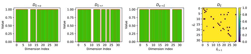
Figure 14: Visualization of estimated structural matrices $D_{\vec{s}{\hbox{\rule[0.0pt]{0.0pt}{0.0pt}}\mkern-4.0mu\hbox{\char 41\relax}}o}$, $D_{\vec{s}{\hbox{\rule[0.0pt]{0.0pt}{0.0pt}}\mkern-4.0mu\hbox{\char 41\relax}}r}$, $D_{a{\hbox{\rule[0.0pt]{0.0pt}{0.0pt}}\mkern-4.0mu\hbox{\char 41\relax}}\vec{s}}$, and $D_{\vec{s}}$ in Car Racing, without the explicit sparsity constraints.

H.2 VizDoom Experiment

We also applied the proposed method to VizDoom (Kempka et al., 2016). VizDoom provides many scenarios and we chose the take cover scenario. Unlike CarRacing, take cover is a discrete control problem with two actions: move left and move right. Reward is +1 at each time step while alive, and the cumulative reward is defined to be the number of time steps the agent manages to stay alive during a episode. Therefore, in order to survive as long as possible, the agent has to learn how to avoid fireballs shot by monsters from the other side of the room. In this task, solving is defined as attaining the average survival time of greater than 750 time steps over 100 consecutive episodes, each running for a maximum of 2100 time steps.

Following a similar setting as in Ha & Schmidhuber (2018), we collected a dataset of 10k random rollouts of the environment, and each runs with random policy until failure. The dimensionality of latent state $\tilde{\vec{s}}_{t}$ is set to $\tilde{d}=32$. We also set $\lambda_{1}\!=\!1$, $\lambda_{2}\!=\!1$, $\lambda_{3}\!=\!1$, $\lambda_{4}\!=\!1$, $\lambda_{5}\!=\!1$, $\lambda_{6}\!=\!6$, $\lambda_{7}\!=\!10$, $\lambda_{8}\!=\!0.1$. By tuning thresholds, we finally reported all the results on the 21-dim ASRs, which achieved the best results in all the experiments.

Analysis of ASRs.

Similar to the analysis in CarRacing, we also visualized the learned $D_{\vec{s}{\hbox{\rule[0.0pt]{0.0pt}{0.0pt}}\mkern-4.0mu\hbox{\char 41\relax}}o}$, $D_{\vec{s}{\hbox{\rule[0.0pt]{0.0pt}{0.0pt}}\mkern-4.0mu\hbox{\char 41\relax}}r}$, $D_{\vec{s}}$, and $D_{a{\hbox{\rule[0.0pt]{0.0pt}{0.0pt}}\mkern-4.0mu\hbox{\char 41\relax}}\vec{s}}$ in VizDoom, as shown in Figure 15. Intuitively, we can see that $D_{\vec{s}{\hbox{\rule[0.0pt]{0.0pt}{0.0pt}}\mkern-4.0mu\hbox{\char 41\relax}}r}$ and $D_{a{\hbox{\rule[0.0pt]{0.0pt}{0.0pt}}\mkern-4.0mu\hbox{\char 41\relax}}\vec{s}}$ have many values close to zero, meaning that the reward is only influenced by a small number of state dimensions, and not many state dimensions are influenced by the action. Furthermore, from $D_{\vec{s}}$, we found that the connections across states are sparse.

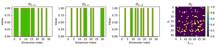
Figure 15: Visualization of estimated structural matrices $D_{\vec{s}{\hbox{\rule[0.0pt]{0.0pt}{0.0pt}}\mkern-4.0mu\hbox{\char 41\relax}}o}$, $D_{\vec{s}{\hbox{\rule[0.0pt]{0.0pt}{0.0pt}}\mkern-4.0mu\hbox{\char 41\relax}}r}$, $D_{a{\hbox{\rule[0.0pt]{0.0pt}{0.0pt}}\mkern-4.0mu\hbox{\char 41\relax}}\vec{s}}$, and $D_{\vec{s}}$ in VizDoom.

Appendix I Detailed Model Architectures

In the car racing experiment, the original screen images were resized to $64\times 64\times 3$ pixels. The encoder consists of three components: a preprocessor, an LSTM, and an MDN. The preprocessor architecture is presented in Figure 16, which takes as input the images, actions and rewards, and its output acts as the input to LSTM. We used 256 hidden units in the LSTM and used a five-component Gaussian mixture in the MDN. The decoder also consists of three components: a current observation reconstructor (Figure 17), a next observation predictor (Figure 18), and a reward predictor (Figure 19). The architecture of the transition/dynamics is shown in Figure 20, and its output is also modelled by an MDN with a five-component Gaussian mixture. In the VizDoom experiment, we used the same image size and the same architectures except that the LSTM has 512 hidden units and the action has one dimension. It is worth emphasising that we applied weight normalization to all the parameters of the architectures above except for the structural matrices $D_{(\cdot)}$.

In DDPG, both actor network and critic network are modelled by two fully connected layers of size 300 with ReLU and batch normalisation. Similarly, in DQN (Mnih et al., 2013) on both ASRs and SSSs, the Q network is also modelled by two fully connected layers of size 300 with ReLU and batch normalisation. However, in DQN on observations, it is modelled by three convolutional layers (i.e., relu conv $32\times 8\times 8$ $\longrightarrow$ relu conv $64\times 4\times 4$ $\longrightarrow$ relu conv $64\times 3\times 3$) followed by two additional fully connected layers of size 64. In DRQN (Hausknecht & Stone, 2015) on observations, we used the same architecture as in DQN on observations but padded an extra LSTM layer with 256 hidden units as the final layer.

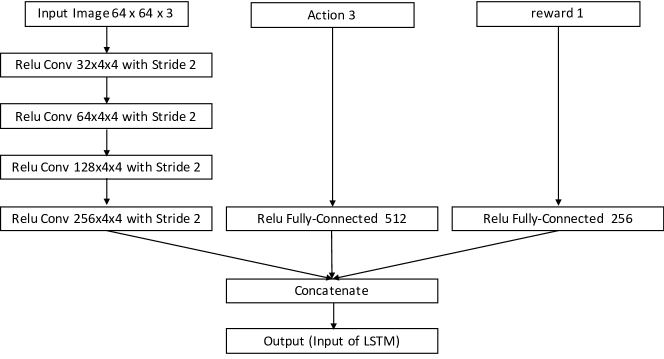
Figure 16: Network architecture of preprocessor.

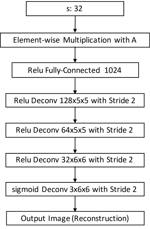
Figure 17: Network architecture of observation reconstruction.

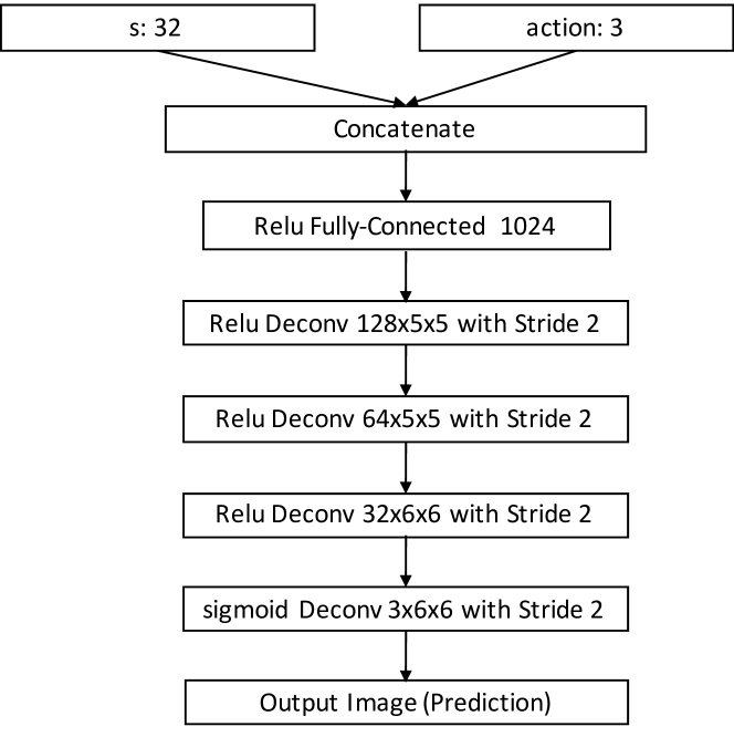
Figure 18: Network architecture of observation prediction.

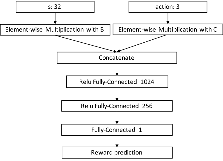
Figure 19: Network architecture of reward.

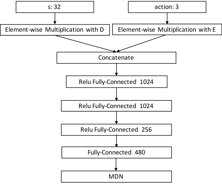
Figure 20: Network architecture of transition/dynamics.

References

- Bengio (2019) Bengio, Y. The consciousness prior. arXiv preprint arXiv:1709.08568, 2019.
- Bishop (1994) Bishop, C. M. Mixture density networks. In Technical Report NCRG/4288, Aston University, Birmingham, UK, 1994.
- Castro (2020) Castro, P. S. Scalable methods for computing state similarity in deterministic Markov decision processes. AAAI, 2020.
- Ebert et al. (2017) Ebert, F., Finn, C., Lee, A. X., and Levine, S. Self-supervised visual planning with temporal skip connections. ArXiv Preprint ArXiv:1710.05268, 2017.
- Gelada et al. (2019) Gelada, C., Kumar, S., Buckman, J., Nachum, O., and Bellemare, M. G. Deepmdp: Learning continuous latent space models for representation learning. In International Conference on Machine Learning (ICML), 2019.
- Ghosh et al. (2019) Ghosh, D., Gupta, A., and Levine, S. Learning actionable representations with goal conditioned policies. ICLR, 2019.
- Gregor et al. (2018) Gregor, K., Papamakarios, G., Besse, F., Buesing, L., and Weber, T. Temporal difference variational auto-encoder. arXiv preprint arXiv:1806.03107, 2018.
- Ha & Schmidhuber (2018) Ha, D. and Schmidhuber, J. World models. In Advances in Neural Information Processing Systems, 2018.
- Hafner et al. (2018) Hafner, D., Lillicrap, T., Fischer, I., Villegas, R., Ha, D., Lee, H., and Davidson, J. Learning latent dynamics for planning from pixels. arXiv preprint arXiv:1811.04551, 2018.
- Hafner et al. (2019) Hafner, D., Lillicrap, T., Ba, J., and Norouzi, M. Dream to control: Learning behaviors by latent imagination. arXiv preprint arXiv:1912.01603, 2019.
- Hafner et al. (2020) Hafner, D., Lillicrap, T., Norouzi, M., and Ba, J. Mastering atari with discrete world models. arXiv preprint arXiv:2010.02193, 2020.
- Hansen (2016) Hansen, N. The CMA evolution strategy: A tutorial. arXiv preprint arXiv:1604.00772, 2016.
- Hausknecht & Stone (2015) Hausknecht, M. and Stone, P. Deep recurrent q-learning for partially observable mdps. In 2015 AAAI Fall Symposium Series, 2015.
- Hochreiter & Schmidhuber (1997) Hochreiter, S. and Schmidhuber, J. Long short-term memory. Neural computation, 9(8):1735–1780, 1997.
- Huang et al. (2019) Huang, B., Zhang, K., Gong, M., and Glymour, C. Causal discovery and forecasting in nonstationary environments with state-space models. In International Conference on Machine Learning (ICML), 2019.
- Huang* et al. (2020) Huang*, B., Zhang*, K., Zhang, J., Ramsey, J., Sanchez-Romero, R., Glymour, C., and Schölkopf, B. Causal discovery from heterogeneous/nonstationary data. JMLR, 21(89), 2020.
- Kaiser et al. (2019) Kaiser, L., Babaeizadeh, M., Milos, P., Osinski, B., Campbell, R. H., Czechowski, K., , and Michalewski, H. Model-based reinforcement learning for Atari. arXiv preprint arXiv:1903.00374, 2019.
- Karl et al. (2016) Karl, M., Soelch, M., Bayer, J., and van der Smagt, P. Deep variational bayes filters: Unsupervised learning of state space models from raw data. arXiv preprint arXiv:1605.06432, 2016.
- Kay et al. (2017) Kay, W., Carreira, J., Simonyan, K., Zhang, B., Hillier, C., Vijayanarasimhan, S., Viola, F., Green, T., Back, T., Natsev, P., et al. The kinetics human action video dataset. arXiv preprint arXiv:1705.06950, 2017.
- Kempka et al. (2016) Kempka, M., Wydmuch, M., Runc, G., Toczek, J., and Jaśkowski, W. ViZDoom: A Doom-based AI research platform for visual reinforcement learning. In IEEE Conference on Computational Intelligence and Games, pp. 341–348, Santorini, Greece, Sep 2016. IEEE. URL http://arxiv.org/abs/1605.02097. The best paper award.
- Kingma & Welling (2013) Kingma, D. P. and Welling, M. Auto-encoding variational bayes. arXiv preprint arXiv:1312.6114, 2013.
- Klimov (2016) Klimov, O. Carracing-v0. http://gym.openai.com/, 2016.
- Krishnan et al. (2015) Krishnan, R., Shalit, U., and Sontag, D. Deep kalman filters. arXiv preprint arXiv:1511.05121, 2015.
- Kulkarni et al. (2016) Kulkarni, T. D., Saeedi, A., Gautam, S., and Gershman, S. J. Deep successor reinforcement learning. arXiv preprint arXiv:1606.02396, 2016.
- Lee et al. (2019) Lee, A. X., Nagabandi, A., Abbeel, P., and Levine, S. Stochastic latent actor-critic: Deep reinforcement learning with a latent variable model. arXiv preprint arXiv:1907.00953, 2019.
- Lesort et al. (2018) Lesort, T., Díaz-Rodríguez, N., Goudou, J. F., and Filliat, D. State representation learning for control: An overview. Neural Networks, 108:379–392, 2018.
- Lillicrap et al. (2015) Lillicrap, T. P., Hunt, J. J., Pritzel, A., Heess, N., Erez, T., Tassa, Y., Silver, D., and Wierstra, D. Continuous control with deep reinforcement learning. arXiv preprint arXiv:1509.02971, 2015.
- Littman & Sutton (2002) Littman, M. L. and Sutton, R. S. Predictive representations of state. In In Advances in neural information processing systems, pp. 1555–1561, 2002.
- Mahadevan & Maggioni (2007) Mahadevan, S. and Maggioni, M. Proto-value functions: A laplacian framework for learning representation and control in markov decision processes. Journal of Machine Learning Research (JMLR), 8:2169–2231, 2007.
- Mnih et al. (2013) Mnih, V., Kavukcuoglu, K., Silver, D., Graves, A., Antonoglou, I., Wierstra, D., and Riedmiller, M. Playing atari with deep reinforcement learning. arXiv preprint arXiv:1312.5602, 2013.
- Mnih et al. (2015) Mnih, V., Kavukcuoglu, K., Silver, D., Rusu, A. A., Veness, J., Bellemare, M. G., Graves, A., Riedmiller, M., Fidjeland, A. K., Ostrovski, G., Petersen, S., Beattie, C., Sadik, A., Antonoglou, I., King, H., Kumaran, D., Wierstra, D., Legg, S., and Hassabis, D. Human-level control through deep reinforcement learning. Nature, 518(7540):529–533, 2015.
- Pearl (2000) Pearl, J. Causality: Models, Reasoning, and Inference. Cambridge University Press, Cambridge, 2000.
- Schölkopf (2019) Schölkopf, B. Causality for machine learning. arXiv preprint arXiv:1911.10500, 2019.
- Shu et al. (2020) Shu, R., Nguyen, T., Chow, Y., Pham, T., Than, K., Ghavamzadeh, M., Ermon, S., and Bui, H. Predictive coding for locally-linear control. In Proceedings of the 37th International Conference on Machine Learning, volume 119 of Proceedings of Machine Learning Research. PMLR, 2020.
- Singh et al. (2004) Singh, S., James, M. R., and Rudary, M. R. Predictive state representations: A new theory for modeling dynamical systems. In In Proceedings of the 20th conference on Uncertainty in artificial intelligence, pp. 512–519, 2004.
- Spirtes et al. (1993) Spirtes, P., Glymour, C., and Scheines, R. Causation, Prediction, and Search. Spring-Verlag Lectures in Statistics, 1993.
- Srinivas et al. (2020) Srinivas, A., Laskin, M., and Abbeel, P. Curl: Contrastive unsupervised representations for reinforcement learning. ICML, 2020.
- Strehl et al. (2007) Strehl, A. L., Diuk, C., and Littman, M. L. Efficient structure learning in factored-state mdps. In AAAI, 2007.
- Sutton (1990) Sutton, R. S. Integrated architectures for learning, planning, and reacting based on approximating dynamic programming. In Machine learning proceedings 1990, pp. 216–224. Elsevier, 1990.
- Sutton & Barto (2018) Sutton, R. S. and Barto, A. G. Reinforcement learning: An introduction. MIT press, 2018.
- Tishby et al. (1999) Tishby, N., Pereira, F. C., and Bialek, W. The information bottleneck method. The 37th annual Allerton Conference on Communication, Control, and Computing, 1999.
- Tsividis et al. (2017) Tsividis, P. A., Pouncy, T., Xu, J. L., Tenenbaum, J. B., and Gershman, S. J. Human learning in atari. In AAAI Spring Symposium Series, 2017.
- Watter et al. (2015) Watter, M., Springenberg, J., Boedecker, J., and Riedmiller, M. Embed to control: A locally linear latent dynamics model for control from raw images. NeurIPS, 2015.
- Wiskott & Sejnowski (2002) Wiskott, L. and Sejnowski, T. J. Slow feature analysis: Unsupervised learning of invariances. Neural Computation, 14(4):715–770, 2002.
- Zhang et al. (2019a) Zhang, A., Lipton, Z. C., Pineda, L., Azizzadenesheli, K., Anandkumar, A., Itti, L., Pineau, J., and Furlanello, T. Learning causal state representations of partially observable environments. arXiv preprint arXiv:1906.10437, 2019a.
- Zhang et al. (2021) Zhang, A., McAllister, R., Calandra, R., Gal, Y., and Levine, S. Learning invariant representations for reinforcement learning without reconstruction. ICLR, 2021.
- Zhang & Spirtes (2011) Zhang, J. and Spirtes, P. Intervention, determinism, and the causal minimality condition. Synthese, 182(3):335–347, 2011.
- Zhang & Hyvärinen (2011) Zhang, K. and Hyvärinen, A. A general linear non-gaussian state-space model: Identifiability, identification, and applications. In Asian Conference on Machine Learning, pp. 113–128, 2011.
- Zhang* et al. (2020) Zhang*, K., Gong*, M., Stojanov, P., Huang, B., Liu, Q., and Glymour, C. Domain adaptation as a problem of inference on graphical models. In NeurIPS, 2020.
- Zhang et al. (2018) Zhang, M., Vikram, S., Smith, L., Abbeel, P., Johnson, M. J., and Levine, S. Solar: deep structured representations for model-based reinforcement learning. arXiv preprint arXiv:1808.09105, 2018.
- Zhang et al. (2019b) Zhang, M., Vikram, S., Smith, L., Abbeel, P., Johnson, M., and Levine, S. Self-supervised visual planning with temporal skip connections. ICML, 2019b.