Computing Hecke Operators for Arithmetic Subgroups of $\mathrm{Sp}_{4}$

1 Introduction

Let $\mathcal{Q}$ be the space of positive definite real symmetric bilinear forms in $n$ variables. This is an open convex cone in the vector space of real symmetric bilinear forms. We identify $\mathcal{Q}$ with the positive definite $n\times n$ symmetric matrices. Let $X_{\mathrm{SL}}$ be the quotient of $\mathcal{Q}$ by homotheties; this is the Riemannian symmetric space for $\mathrm{SL}_{n}(\mathbb{R})$. The group $\mathrm{SL}_{n}(\mathbb{Z})$ acts properly discontinuously on $X_{\mathrm{SL}}$, generalizing the classical action of $\mathrm{SL}_{2}(\mathbb{Z})$ on the upper half-plane. Let $\Gamma_{\mathrm{SL}}$ be an arithmetic subgroup of $\mathrm{SL}_{n}(\mathbb{Z})$. Let $\rho$ be a suitable local system of coefficients on $X_{\mathrm{SL}}$; the first lines of Section 2.5 will specify which $\rho$ we use.

The paper [12] introduced an algorithm for computing Hecke operators on the equivariant cohomology $H^{i}_{\Gamma_{\mathrm{SL}}}(X_{\mathrm{SL}};\rho)$. When $\rho$ is over a field of characteristic zero, or of characteristic not dividing the order of any torsion element of $\Gamma_{\mathrm{SL}}$, this is isomorphic to the ordinary cohomology $H^{i}(\Gamma_{\mathrm{SL}}\backslash X_{\mathrm{SL}};\rho)$. The algorithm in [12] works for any $\rho$ and for all $i=0,1,2,\dots,\operatorname{\mathrm{vcd}}(\Gamma_{\mathrm{SL}})$, where $\operatorname{\mathrm{vcd}}(\Gamma_{\mathrm{SL}})=\dim(\mathcal{Q})-n=\frac{1}{2}n(n-1)$ is the virtual cohomological dimension.

The present paper extends [12] to the symplectic group for $n=4$. Let $\mathrm{Sp}_{4}(\mathbb{R})$ be the subgroup of $\mathrm{SL}_{4}(\mathbb{R})$ that preserves the skew-symmetric bilinear form with matrix

$$\Omega=\begin{bmatrix}0&0&0&1\\ 0&0&1&0\\ 0&-1&0&0\\ -1&0&0&0\end{bmatrix}.$$

Let $X$ be the Riemannian symmetric space for $\mathrm{Sp}_{4}(\mathbb{R})$. This is the submanifold of $\mathcal{Q}$ consisting of those $A\in\mathcal{Q}$ satisfying the symplectic condition $A\Omega A^{t}=\Omega$. Working mod homotheties, $X$ is embedded in $X_{\mathrm{SL}}$. Let $\Gamma=\Gamma_{\mathrm{SL}}\cap\mathrm{Sp}_{4}(\mathbb{Z})$, where we always suppose $\Gamma_{\mathrm{SL}}$ is chosen so that $\Gamma$ is an arithmetic subgroup of $\mathrm{Sp}_{4}(\mathbb{Z})$. If $\Gamma$ is torsion free, $\Gamma\backslash X$ is a smooth complex algebraic variety called a Siegel modular threefold.

In this paper, we outline an algorithm for computing Hecke operators on the equivariant cohomology $H^{i}_{\Gamma}(X;\rho)$. The algorithm works for any local coefficient system $\rho$ and for all $i$.

1.1 Well-Tempered Complexes

The algorithm for $\mathrm{SL}_{n}$ in [12] uses the well-tempered complex $\widetilde{W}^{+}$. This is a regular cell complex of dimension $\operatorname{\mathrm{vcd}}(\Gamma_{\mathrm{SL}})+1$. For a certain $\tau_{0}>1$, it is a fibration $\widetilde{W}^{+}\to[1,\tau_{0}^{2}]$, where the coordinate $\tau$ in the base is called the temperament. Let $\widetilde{W}_{\tau}$ be the fiber over $\tau$. Each fiber is a contractible cell complex of dimension $\operatorname{\mathrm{vcd}}(\Gamma_{\mathrm{SL}})$ on which $\Gamma_{\mathrm{SL}}$ acts with finitely many orbits of cells. The fiber $\widetilde{W}_{1}$ is the well-rounded retract of [2]. As $\tau$ varies, there are a finite number of critical temperaments $\tau^{(i)}$ where the cell structure of the fibers of $\widetilde{W}^{+}$ abruptly changes. On the intervals between consecutive critical temperaments, the cell structure does not change from fiber to fiber. See Figures 1 and 2 below for examples.

This paper’s new algorithm for $\mathrm{Sp}_{4}$ uses a subcomplex $\widetilde{V}^{+}$ of $\widetilde{W}^{+}$ for $n=4$. This $\widetilde{V}^{+}$ is a regular cell complex of dimension $\operatorname{\mathrm{vcd}}{\Gamma_{\mathrm{SL}}}+1$ and is a fibration $\widetilde{V}^{+}\to[1,\tau_{0}^{2}]$. Every fiber has dimension $\operatorname{\mathrm{vcd}}{\Gamma_{\mathrm{SL}}}=6$. The complex $\widetilde{V}^{+}$ and all its fibers admit an action of $\Gamma$ with only finitely many orbits of cells. We define the fiber $\widetilde{V}_{1}$ in Definition 5; in the last Section, we discuss how to compute the other fibers.

The $\widetilde{V}_{\tau}$ are not the complexes we would prefer to use. [10] introduced a cell complex $\widetilde{V}$ (called $W$ in that paper) whose dimension is $4$, the true vcd of $\mathrm{Sp}_{4}(\mathbb{Z})$. The complex $\widetilde{V}$ is contractible and hence acyclic, and $\mathrm{Sp}_{4}(\mathbb{Z})$ acts on it with only finitely many orbits of cells. In [9], the combinatorics of the cells of $\widetilde{V}$ are described in terms of classical projective configurations in the symplectic projective three-space $\mathbb{P}^{3}(\mathbb{Q})$ endowed with the form $\Omega$. Our $\widetilde{V}_{1}$ in this paper is a thickening of $\widetilde{V}$, of dimension $6$. More precisely, it follows from [10] that there is an $\mathrm{Sp}_{4}(\mathbb{Z})$-equivariant embedding of $\widetilde{V}$ as a subcomplex of the first barycentric subdivision of $\widetilde{V}_{1}$.

Our main theorem is Theorem 6, which says that $\widetilde{V}$ and $\widetilde{V}_{1}$ have the same cohomology. This implies that $\widetilde{V}_{1}$ is itself an acyclic cell complex on which $\mathrm{Sp}_{4}(\mathbb{Z})$ acts with only finitely many stabilizers of cells. As such, $\widetilde{V}_{1}$ is suitable for computing the equivariant cohomology of $\Gamma$. The advantage of $\widetilde{V}_{1}$ over $\widetilde{V}$ is that we can extend $\widetilde{V}_{1}$ to $\widetilde{V}^{+}$, obtaining a Hecke algorithm along the lines of [12]. The proof of Theorem 6 appears in Section 3.

In Section 4, we outline a computational method which, conjecturally, would construct the fibers $\widetilde{V}_{\tau}$ for $\tau>1$ and show they are contractible. Once these computations were carried out, the rest of the Hecke operator algorithm would proceed as in [12]. We emphasize that Section 4 is speculative, unlike the earlier sections. Details for Section 4 will appear in a later paper.

We summarize our notation.

$\widetilde{W}^{+}$	well-tempered complex for $\mathrm{SL}_{4}(\mathbb{R})$
$\widetilde{W}_{1}$	well-rounded retract for $\mathrm{SL}_{4}(\mathbb{R})$ at temperament $1$ for $\widetilde{W}^{+}$
$\widetilde{V}$	contractible complex for $\mathrm{Sp}_{4}(\mathbb{R})$ from [10]
$\widetilde{V}^{+}$	the new acyclic subcomplex of $\widetilde{W}^{+}$ introduced in this paper
$\widetilde{V}_{1}$	cell complex at the first temperament for $\widetilde{V}^{+}$

1.2 Acknowledgments

Avner Ash’s paper [2] is foundational for both [12] and this paper. Paul Gunnells suggested to us that combining [10] and [12] might give a Hecke operator algorithm for $\mathrm{Sp}_{4}$. We thank both of them for these and many other helpful conversations. We also thank Robert MacPherson and Dan Yasaki.

2 The Well-Tempered Complex for $\mathrm{SL}_{n}(\mathbb{Z})$

Here is a summary of [12]. That paper concerns $\mathrm{GL}_{n}$ over any division algebra $D$ of finite dimension over $\mathbb{Q}$. We now specialize to $D=\mathbb{Q}$, so that all arithmetic groups $\Gamma$ are subgroups of $\Gamma_{0}=\mathrm{GL}_{n}(\mathbb{Z})$. Throughout this Section 2, we deal only with the objects called $X_{\mathrm{SL}}$ and $\Gamma_{\mathrm{SL}}$ in the Introduction, so we drop the subscripts $\mathrm{SL}$ from those symbols.

A $\mathbb{Z}$-lattice in $\mathbb{R}^{n}$ is a finitely generated discrete subgroup that contains an $\mathbb{R}$-basis. $G=\mathrm{GL}_{n}(\mathbb{R})$ acts on the right on row vectors in $\mathbb{R}^{n}$, and $\Gamma_{0}=\mathrm{GL}_{n}(\mathbb{Z})$ stabilizes the standard lattice $L_{0}=\mathbb{Z}^{n}$. Let $Y=\Gamma\backslash G$. We view $Y$ as a space of lattices, whose elements are $L_{0}g$; the lattices have extra structure, such as a level structure, when $\Gamma\subsetneqq\Gamma_{0}$. The group preserving the standard inner product $\langle\,,\,\rangle$ on $\mathbb{R}^{n}$ is the maximal compact subgroup $K=\mathrm{O}_{n}\subset G$, and $X=G/K$ is the corresponding symmetric space.

2.1 The Well-Rounded Retract

Definition 1.

Let $L=L_{0}g\in Y$. The arithmetic minimum of $L$ is $m(L)=\min\{\langle x,x\rangle\mid x\in L-\{0\}\}$. The minimal vectors are $M(L)=\{x\in L\mid\langle x,x\rangle=m(L)\}$. We say $L$ is well rounded if $M(L)$ spans $\mathbb{R}^{n}$. The set of well-rounded lattices in $Y$ with minimum 1 is denoted $\widehat{W}$.

The functions $m$ and $M$ are $K$-invariant. Hence $\widehat{W}$ is $K$-invariant.

Theorem 1 ([2, Thm. 2.11]).

$W=\widehat{W}/K$ is a strong deformation retract of $Y/K$. It is compact and of dimension $\operatorname{\mathrm{vcd}}\Gamma_{0}$. The universal cover $\widetilde{W}$ of $W$ is a locally finite regular cell complex in $X$ on which $\Gamma_{0}$ acts cell-wise with finite stabilizers of cells. This cell structure has a natural barycentric subdivision which descends to a finite cell complex structure on $W$.

Definition 2.

$W=\widehat{W}/K$ is the well-rounded retract.

2.2 A Family of Retracts

The paper [12] extends Theorem 1 by adding an extra dimension to $Y$. It starts with the trivial bundle $Y\times I$ over an interval $I$, where $G$ acts fiberwise on $Y\times I$. There is a corresponding bundle isomorphism $(Y\times I)/K\cong(Y/K)\times I$ with fibers $Y/K$.

In order to generalize the construction of Theorem 1 and build a family of retracts, one needs the concept of a family of weights. The quotient $\mathbb{P}^{n-1}(\mathbb{Q})/\Gamma$ is finite. A set of weights for $\Gamma$ is a function $\varphi:\mathbb{P}^{n-1}(\mathbb{Q})/\Gamma\to\mathbb{R}_{+}$. Such a $\varphi$ defines a set of weights for $L_{0}$, also denoted $\varphi$, by $\varphi(x)=\varphi(\mathbb{Q}x)$. This is a $\Gamma$-invariant function $L_{0}-\{0\}\to\mathbb{R}_{+}$. For $L=L_{0}g$, a set of weights $\varphi$ for $L_{0}$ defines a set of weights for $L$, by $\varphi^{L}(xg)=\varphi(x)$, with $\varphi^{L}:L-\{0\}\to\mathbb{R}_{+}$.

A one-parameter family of weights for $L_{0}$ is a map $\varphi_{\tau}:(L_{0}-\{0\})\times I\to\mathbb{R}^{+}$ which is a $\Gamma$-invariant set of weights for any given $\tau$, and for which $\varphi_{\tau}(x)$ is real analytic in $\tau$ for any given $x$. We normalize $\varphi_{\tau}$ by dividing through by a positive real scalar, which depends continuously on $\tau$, so that the maximum of $\varphi_{\tau}$ is 1 for all $\tau$. A one-parameter family of weights $\varphi_{\tau}$ determines $\varphi^{L}_{\tau}$ for $L=L_{0}g$ by $\varphi^{L}_{\tau}(xg)=\varphi_{\tau}(x)$. As a function of $\tau$, the arithmetic minimum is given by $m(L)=\min\{\varphi_{\tau}^{L}(x)\langle x,x\rangle\mid x\in L-\{0\}\}$, with minimal vectors

$$M(L)=\{x\in L\mid\varphi_{\tau}^{L}(x)\langle x,x\rangle=m(L)\}.$$ (1)

The spaces $\widehat{W}_{\tau}$ and $W_{\tau}=\widehat{W}_{\tau}/K$ for any given $\tau$ are defined similarly. By [2, Thm. 2.11], there is a strong deformation retraction $R_{\tau}(t)$ of the fiber over $\tau$ onto $W_{\tau}$. In fact, more is true:

Theorem 2 ([12]).

$R_{\tau}(t)$ is a continuous map $((Y\times I)/K)\times[0,1]\to(Y\times I)/K$.

Corollary.

$\{(w\times\tau)/K\mid\tau\in I,w\in\widehat{W}_{\tau}\}$ is a strong deformation retract of $(Y\times I)/K$. It has dimension $\operatorname{\mathrm{vcd}}\Gamma$. It is compact if $I$ is compact. The map from the retract to $I$ is a fibration.

2.3 Hecke Correspondences

We review Hecke correspondences for $\mathrm{GL}_{n}$, following [14, §3.1 and p. 76]. Define $\Delta=\{a\in G\mid L_{0}a\subseteq L_{0}\}$. Then $\Gamma_{0}\subset\Delta$, and $\Delta$ is the sub-semigroup of $\mathrm{GL}_{n}(\mathbb{Q})$ with integer entries. The arithmetic group $\Gamma=\Gamma_{0}\cap a^{-1}\Gamma_{0}a$ is the common stabilizer in $G$ of $L_{0}$ and its sublattice $M_{0}=L_{0}a$. One calls $(\Gamma_{0},\Delta)$ a Hecke pair.

A point in $\Gamma_{0}\backslash X$ has the form $\Gamma_{0}gK$ with $g\in G$. Define two maps

(2)

by $p:\Gamma gK\mapsto\Gamma_{0}gK$ and $q:\Gamma gK\mapsto\Gamma_{0}agK$. The Hecke correspondence $T_{a}$ is the one-to-many map $\Gamma_{0}\backslash X\to\Gamma_{0}\backslash X$ given by

$$T_{a}=q\circ p^{-1}.$$

It sends one point of $\Gamma_{0}\backslash X$ to $[\Gamma_{0}:\Gamma]$ points of $\Gamma_{0}\backslash X$, counting multiplicities.

The Hecke algebra for the Hecke pair $(\Gamma_{0},\Delta)$ is the free abelian group on the set of correspondences $T_{a}$ for $a\in\Delta$, with multiplication defined by the composition of correspondences. This is equivalent to the traditional definition as the algebra of double cosets $\Gamma_{0}a\Gamma_{0}$ for $a\in\Delta$ [14, p. 54].

For a prime $\ell\in\mathbb{Z}$ and for $k\in\{1,\dots,n\}$, define

$$T_{\ell,k}=T_{a}\quad\mathrm{for\ }a=\mathrm{diag}(\underbrace{1,\dots,1}_{n-k\mathrm{\ times}},\underbrace{\ell,\dots,\ell}_{k\mathrm{\ times}}).$$

The Hecke algebra is generated by the $T_{\ell,k}$ for all primes $\ell$ and $k\in\{1,\dots,n\}$. If instead $G=\mathrm{SL}_{n}(\mathbb{R})$ and $\Gamma_{0}=\mathrm{SL}_{n}(\mathbb{Z})$, then $\Delta$ is the semigroup with entries in $\mathbb{Z}$ and positive determinant, and the Hecke algebra is generated by the same $T_{\ell,k}$ [14, §3.2].

   

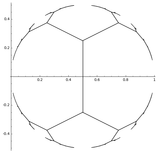
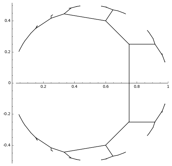
Figure 1: The well-rounded retract for $\mathrm{GL}_{2}(\mathbb{Z})$, and its translate by $T_{2}$.

2.3.1 Example for $n=2$

In the Figures, we will present a running example for $\Gamma_{0}=\mathrm{GL}_{2}(\mathbb{Z})$. The left-hand side of Figure 1 shows the complex $\widetilde{W}$ for $\mathrm{GL}_{2}(\mathbb{Z})$. Here $X$ is the unit disc, which is the Klein model of the symmetric space. $\widetilde{W}$ is a tree. $\Gamma_{0}$ acts on the tree, acting transitively on both the vertices and the edges.

The right-hand side of Figure 1 shows the image of $\widetilde{W}$ under $T_{2}=T_{2,1}$. It is a tree, and $\Gamma$ is the largest subgroup of $\Gamma_{0}$ that acts on it. To compute $T_{2}$, we will build a one-parameter family of trees that interpolates between the two sides of Figure 1 in a $\Gamma$-equivariant way. In the next section, we explain how to use Theorem 2 to build the family. Figure 2 will show some members of the family.

2.4 The Well-Tempered Complex

Our choice of $L_{0}$ determined the well-rounded retract for $\Gamma_{0}$. Now fix $a\in\Delta$, and let $\Gamma=\Gamma_{0}\cap a^{-1}\Gamma_{0}a$ as before. The well-tempered complex $W^{+}$ will be determined by both $L_{0}$ and $a$, and will naturally admit an action by $\Gamma$.

Let $M_{0}=L_{0}a$. By a standard calculation based on how $M_{0}$ and $\Gamma$ are defined in terms of $a$, the next definition gives a set of weights $\varphi_{\tau}$ for $\Gamma$. We use this particular set of weights for the rest of the paper.

Definition 3.

For $x\in L_{0}-\{0\}$ and $\tau\geqslant 1$, define

$$\varphi_{\tau}(x)=\left\{\begin{array}[]{cl}\varphi(x)&\quad\mathrm{if\ }x\in M_{0}-\{0\},\\ \tau^{2}\varphi(x)&\quad\mathrm{if\ }x\notin M_{0}.\end{array}\right.$$

Remark.

The idea here comes from $m(L)$ in Definition 1. The weighted squared length of a vector $x\in L$ is $\varphi^{L}(x)\langle x,x\rangle$. The squared length $\langle x,x\rangle$ scales by $c^{2}$ when we multiply $x$ by $c\in\mathbb{R}$. By multiplying the weight by $\tau^{2}$ when $x\notin M_{0}$, we mimic the effect of scaling the length of $x$ linearly by $\tau$. We pretend $x\notin M_{0}$ gets “longer by lies”, linearly. When $x\in M_{0}$, we do not pretend to change the length.

Choose $\tau_{0}>1$, and let $I=[1,\tau_{0}]$. The well-tempered complex depends on $\tau_{0}$, but [12] shows that the complexes for two different $\tau_{0}$ are isomorphic when $\tau_{0}$ is sufficiently large.

Definition 4.

The well-tempered complex $W^{+}$ for $L_{0}$, $\varphi$, and $a$ is the image of $(Y\times[1,\tau_{0}])/K$ under the retraction $R_{\tau}(t)$ of Theorem 2, where $\varphi_{\tau}$ is as in Definition 3.

Theorem 3 ([12, Thm. 4.33]).

The universal cover $\widetilde{W}^{+}$ of the well-tempered complex $W^{+}$ is a locally finite regular cell complex on which $\Gamma$ acts cell-wise with finite stabilizers of cells. This cell structure has a natural barycentric subdivision which descends to a finite cell complex structure on $W^{+}$.

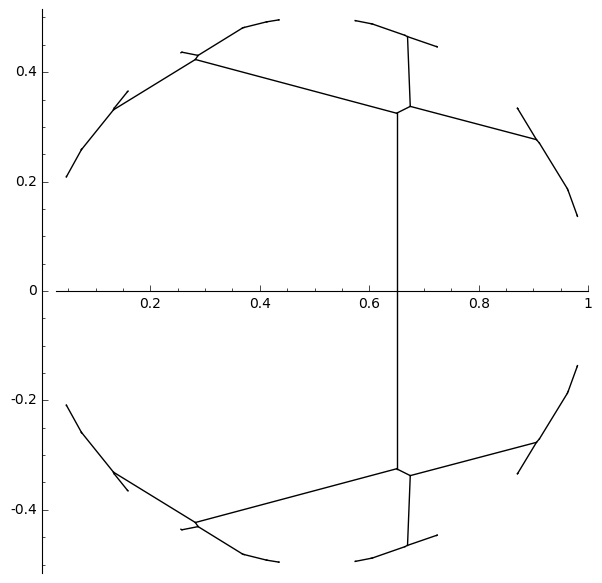
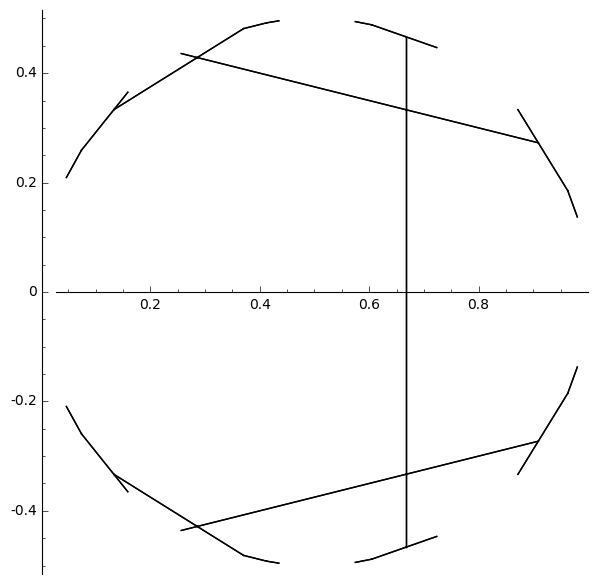
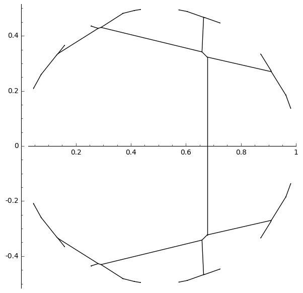
Figure 2: How the fiber continuously deforms in the well-tempered complex.

In the original well-rounded retract $\widetilde{W}$, the cells are indexed by their sets of minimal vectors $M$, each of which is a finite subset of $L_{0}-\{0\}$. In the well-tempered complex, cells are indexed by pairs consisting of sets $M$ and a set of temperaments. The proof of Theorem 3 in [12] shows that there are a finite number of critical temperaments $\tau^{(i)}$ with $1=\tau^{(0)}<\tau^{(1)}<\cdots<\tau^{(r)}=\tau_{0}$. The cells $\sigma$ of Theorem 3 are cut into closed pieces along the hyperplanes $\tau=\tau^{(i)}$ for $i=0,\dots,r$. Each non-empty cell of the refinement is indexed by a pair. The pair is $(M,[\tau^{(i-1)},\tau^{(i)}])$ if the projection of the cell to the $\tau$-coordinate is $[\tau^{(i-1)},\tau^{(i)}]$. The pair is $(M,[\tau^{(i)},\tau^{(i)}])$ if the projection is $\{\tau^{(i)}\}$. We will write $[\tau,\tau^{\prime}]$ as shorthand for both $[\tau^{(i-1)},\tau^{(i)}]$ and $[\tau^{(i)},\tau^{(i)}]$.

2.4.1 Example for $n=2$

We continue the example from Section 2.3.1 for $T_{2}$ for $\Gamma_{0}=\mathrm{GL}_{2}(\mathbb{Z})$. The critical temperaments turn out to be $\tau^{(i)}=1,2,4$. The well-tempered complex $\widetilde{W}^{+}$ has dimension 2. Figure 1 showed the slices of $\widetilde{W}^{+}$ at $\tau=1$ and $4$. Figure 2 shows the slices at $\tau=2-\varepsilon$, $2$, and $2+\varepsilon$ for a small $\varepsilon>0$. It illustrates how the cell structure changes at $\tau=2$.

2.4.2 Hecketopes

Voronoi’s reduction theory [15] gives a way to make the well-rounded retract $\widetilde{W}$. The Voronoi cones of [15] are the cones over the faces of a Voronoi polyhedron. The cells of $\widetilde{W}$ are unions of cells in a certain subdivision of the Voronoi cones, and, in fact, the cells of $\widetilde{W}$ are dual to the faces of the Voronoi polyhedron. In the same way, the well-tempered cells of $\widetilde{W}^{+}$ are dual to a generalization of the Voronoi polyhedron called the Hecketope. Section 6 of [12] describes the Hecketope in full, presenting practical algorithms for finding the cells of $\widetilde{W}^{+}$ along with the critical temperaments and the indexing data $(M,[\tau,\tau^{\prime}])$.

2.4.3 The first and last temperament

For the $a$ giving the Hecke operator $T_{\ell,k}$, [12] sets $\tau_{0}=\ell$ and shows there is then a simple relationship between the fibers of the well-tempered complex over $\tau_{0}$ and over $1$:

Theorem 4 ([12]).

For any $\tau\geqslant\tau_{0}$, the map $X\to X$ given by $gK\mapsto a^{-1}gK$ descends mod $\Gamma$ to give a cell-preserving homeomorphism from the well-rounded retract $W_{1}$ over $1$ to the well-rounded retract $W_{\tau}$ over $\tau$. If a cell over $\tau=1$ is $\sigma_{1}(Q)$ with index set $Q\subset L_{0}-\{0\}$, then the cell that corresponds to $\sigma_{1}(Q)$ under the homeomorphism has index set $Qa$.

We call the endpoints of $[1,\tau_{0}]$ the first and last temperaments, respectively.

2.5 Computing Hecke Operators

Let the Hecke pair $(\Gamma_{0},\Delta)$ be as above. Let $\rho$ be any left $\mathbb{Z}\Delta$-module. (We often take the tensor product of $\rho$ with a field like $\mathbb{Q}$ or $\mathbb{F}_{p}$.) There is a natural left action of the Hecke algebra on the equivariant cohomology $H^{*}_{\Gamma_{0}}(X;\rho)$ [3, §1.1]. For $a\in\Delta$, the action of the Hecke correspondence $T_{a}$ on the cohomology is called the Hecke operator associated to $a$, and it will also be denoted $T_{a}$. It is defined to be $p_{*}q^{*}$ in a diagram derived from (2):

(3)

The map $q^{*}:H^{*}_{\Gamma_{0}}(X;\rho)\to H^{*}_{\Gamma}(X;\rho)$ is the natural pullback map for $q$. The map $p_{*}:H^{*}_{\Gamma}(X;\rho)\to H^{*}_{\Gamma_{0}}(X;\rho)$ is the transfer map [5, III.9] for $p$, which is defined because $\Gamma=\Gamma_{0}\cap a^{-1}\Gamma_{0}a$ has finite index in $\Gamma_{0}$.

We now give an algorithm that uses the well-tempered complex to compute $T_{a}$. To compute equivariant cohomology, we may use any acyclic cell complex on which $\Gamma_{0}$ acts. The fiber $\widetilde{W}_{\tau}$ of the well-tempered complex $\widetilde{W}^{+}$ over any $\tau$ is a strong deformation retract of $X$, hence acyclic. This holds in particular for the fibers $\widetilde{W}_{\tau^{(i)}}$ over the critical temperaments $\tau^{(i)}$, and for the inverse image of the closed interval between two consecutive critical temperaments. Indeed, $\widetilde{W}_{[\tau^{(i-1)},\tau^{(i)}]}$ has dimension one higher than the vcd, but its cohomology in degree vcd$+1$ will be zero.

First, we compute $p_{*}$. We use $\tau=1$, the first temperament, when working with $p$. The retracts $\widetilde{W}$ and $\widetilde{W}_{1}$ are equal by definition. $\Gamma_{0}$ acts on $\widetilde{W}$, and the smaller group $\Gamma$ acts on $\widetilde{W}_{1}$. Computing the transfer map is straightforward. (In practice it is tricky to get the orientation questions correct. This is true for all the cells, and especially for the cells with non-trivial stabilizer subgroups. This comment applies to all the computations in this paper.)

Next, we compute $q^{*}$. The pullback map is natural on cohomology, but we must account for the factor of $a$ in the definition of $q$. The key is to use the last temperament $\tau_{0}$ when working with $q$. We compute $H^{*}_{\Gamma}(X;\rho)$ as $H^{*}_{\Gamma}(\widetilde{W}_{\tau_{0}};\rho)$. By Theorem 4, there is a homeomorphism of cell complexes $\widetilde{W}_{\tau_{0}}\to\widetilde{W}_{1}$, from the last temperament to the first, given by multiplication by $a$. As we saw for $p$, $\widetilde{W}_{1}$ equals $\widetilde{W}$. Thus there is a cellular map which enables us to compute $q^{*}:H^{*}_{\Gamma_{0}}(\widetilde{W};\rho)\to H^{*}_{\Gamma}(\widetilde{W}_{\tau_{0}};\rho)$.

Computing only $p_{*}$ and $q^{*}$ does not give us the Hecke operator. The map of Theorem 4 involves dividing or multiplying by $a$. It is not a map of $\Gamma$-modules, because $a\in\Delta$ but $a\notin\Gamma$ in general. For this reason, we cannot directly map $H^{*}_{\Gamma}(\widetilde{W}_{\tau_{0}};\rho)$ to $H^{*}_{\Gamma}(\widetilde{W}_{1};\rho)$. To overcome this last difficulty, we use the whole well-tempered complex to define a chain of morphisms and quasi-isomorphisms. For $i=1,\dots,i_{r}$, in the portion $\widetilde{W}_{[\tau^{(i-1)},\tau^{(i)}]}$ over the fibers $\tau\in[\tau^{(i-1)},\tau^{(i)}]$, define the closed inclusions of the fibers on the left and right sides:

$$\widetilde{W}_{\tau^{(i-1)}}\xhookrightarrow{l^{(i-1)}}\widetilde{W}_{[\tau^{(i-1)},\tau^{(i)}]}\xhookleftarrow{r^{(i)}}\widetilde{W}_{\tau^{(i)}}$$

By Theorems 2 and 3, we can compute the pullbacks $(l^{(i-1)})^{*}$ and the pushforwards $(r^{(i)})_{*}$ on $H^{*}_{\Gamma}(\dots;\rho)$. The pullback is a naturally defined cellular map. The pushforward $(r^{(i)})_{*}$ is a quasi-isomorphism, the inverse of the pullback $(r^{(i)})^{*}$; we compute the pullback at the cochain level using the cellular map, then invert the map on cohomology.

We summarize our algorithm as a theorem.

Theorem 5 ([12]).

With notation as above, the Hecke operator $T_{a}$ on equivariant cohomology (3) may be computed in finite terms as the composition

$$p_{*}{l^{(0)}}^{*}r^{(1)}_{*}{l^{(1)}}^{*}r^{(2)}_{*}\cdots{l^{(i_{r}-1)}}^{*}r^{(i_{r})}_{*}q^{*}.$$ (4)

2.6 Cohomology of Subgroups

Let $\Gamma^{\prime}\subseteq\Gamma_{0}$ be an arithmetic subgroup. We wish to compute Hecke operators on the equivariant cohomology $H^{*}_{\Gamma^{\prime}}(X;\rho)$ for any $\Gamma^{\prime}$. By Shapiro’s Lemma [5, III.6.2], $H^{*}_{\Gamma^{\prime}}(X;\rho)\cong H^{*}_{\Gamma_{0}}(X;\mathrm{Coind}_{\Gamma^{\prime}}^{\Gamma_{0}}\rho)$. We use Theorem 5 to compute the latter.

3 A Subcomplex for $\mathrm{Sp}_{4}(\mathbb{Z})$

3.1 PL Embedding Lemma

The well-rounded retract $\widetilde{W}$ for $\mathrm{SL}_{4}(\mathbb{R})$ has real dimension 6. All of its 6-cells are equivalent modulo $\mathrm{SL}_{4}(\mathbb{Z})$; as a representative 6-cell, we may choose the cell $\sigma$ whose minimal vectors are the columns of the $4\times 4$ identity matrix [15].

Definition 5.

Denote by $\widetilde{V}_{1}$ the following closed subcomplex of $\widetilde{W}$:

$$\widetilde{V}_{1}=\left\{\gamma\cdot\sigma\;|\;\gamma\in\mathrm{Sp}_{4}(\mathbb{Z})\right\}.$$

$\widetilde{V}_{1}$ has an action of $\mathrm{Sp}_{4}(\mathbb{Z})$, but not an action of $\mathrm{SL}_{4}(\mathbb{Z})$. We will denote by $\alpha$ a closed cell in $\widetilde{V}_{1}$ that is a non-empty intersection of the form

$$\alpha=\alpha_{i_{1}\cdots i_{k}}=\bigcap^{k}_{j=1}\gamma_{i_{j}}\sigma,\quad\gamma_{i_{j}}\in\mathrm{Sp}_{4}(\mathbb{Z}).$$ (5)

We will use this notation to suppress indices wherever they do not play a crucial role.

Let $\widetilde{V}$ be the retract for $\mathrm{Sp}_{4}(\mathbb{R})$ constructed in [10]. The following lemma allows us to identify $\widetilde{V}$ with its embedded image inside the subcomplex $\widetilde{V}_{1}$ of $\widetilde{W}$ that we have just defined.

Lemma 1.

There exists a PL-embedding $\widetilde{V}\rightarrow\widetilde{V}_{1}$.

Proof.

In both $\widetilde{W}$ and $\widetilde{V}$, the cells are in one-to-one correspondence with their sets of minimal vectors. In either cell complex, a cell $\alpha$ is a face of $\beta$ if and only if the set of minimal vectors for $\alpha$ contains the set of minimal vectors for $\beta$, by [11] and [10]. Denote by $\mathscr{C}_{\textup{SL}}$ the poset of the sets of minimal vectors for $\widetilde{W}$ and by $\mathscr{C}_{\textup{Sp}}$ the corresponding poset for $\widetilde{V}$. These are ranked posets, where the rank of an item is the dimension of the corresponding cell. By the construction in [10], there is an injective homomorphism of ranked posets $\mathscr{C}_{\textup{Sp}}\rightarrow\mathscr{C}_{\textup{SL}}$. Since geometric realization is a faithful functor, it follows that there is PL-embedding $\widetilde{V}\rightarrow\widetilde{W}$, whose image is contained in $\widetilde{V}_{1}$. ∎

3.2 Thickening Theorem

We remarked in the introduction that the PL embedding $\widetilde{V}\rightarrow\widetilde{V}_{1}$ is a thickening of $\widetilde{V}$, raising the dimension from 4 to 6. The main theorem of this Section is that the two spaces have the same topology.

Theorem 6.

The PL embedding $\widetilde{V}\rightarrow\widetilde{V}_{1}$ induces an isomorphism on cohomology. In particular, $\widetilde{V}_{1}$ is acyclic.

3.3 Local Contractibility

We need a local result about contractibility. In the next section, this will be extended to prove the global result that $\widetilde{V}_{1}$ is acyclic.

Proposition 1.

For any $\alpha$ of the form (5), $\alpha\cap\widetilde{V}$ is a contractible subcomplex of $\widetilde{V}_{1}$.

Proof.

Without loss of generality, we may assume $\alpha$ is a face of $\sigma$. Indeed, by its definition, $\widetilde{V}_{1}$ is invariant under $\mathrm{Sp}_{4}(\mathbb{Z})$, so we may replace $\alpha$ by $\gamma\alpha$ for any $\gamma\in\mathrm{Sp}_{4}(\mathbb{Z})$. After this replacement, we may take $\gamma_{i_{1}}=I$.

Let $\mathscr{R}$ be the set of all cells $\widetilde{W}$ which have the form $\gamma\sigma$ for some $\gamma\in\mathrm{Sp}_{4}(\mathbb{Z})$ and such that $\gamma\sigma\cap\sigma\neq\varnothing$. By definition, $\mathscr{R}$ is a subset of $\widetilde{V}_{1}$. It is finite, by the local finiteness of $\widetilde{W}_{1}$. Every non-empty $\alpha$ of the form (5) will have all of its $\gamma_{i_{j}}\sigma$ in $\mathscr{R}$, given the constraint $\alpha\subseteq\sigma$.

We use a computer to enumerate and store $\mathscr{R}$, as follows. Enumerate all the faces $\beta$ of $\sigma$ (these have dimensions $0,\dots,6$). For each $\beta$, let $M$ be the set of its minimal vectors; $M$ is a subset of $\mathbb{Z}^{4}$ containing between 4 and 12 vectors. (We find $M$ based on the tables in [11]. Vectors $\vec{x}$ and $-\vec{x}$ in $M$ are counted only once.) For each $M$, consider all $\binom{|M|}{4}$ four-element subsets $M_{4}$. We test whether we can permute the columns of $M_{4}$, and multiply zero or more of its columns by $-1$, to make $M_{4}\in\mathrm{Sp}_{4}(\mathbb{Z})$. If the test passes, then $\gamma=M_{4}\in\mathrm{Sp}_{4}(\mathbb{Z})$ is such that $\gamma\sigma\in\mathscr{R}$.

Next, we compute all $\alpha$’s by computing all $k$-fold intersections of cells in $\mathscr{R}$. We use a hash table whose value is an $\alpha$ as in (5), and whose key $M$ is the union of the minimal vectors for the $\gamma_{i_{j}}$ appearing in the intersection. (In other words, $M$ is the union of the column vectors $\vec{x}$ in the matrices $\gamma_{i_{1}}=I$, $\gamma_{i_{2}}$, …, $\gamma_{i_{k}}$, and $-\vec{x}$ too.) We use a loop to fill the hash table first with ($k=1$)-fold intersections (which means $\gamma_{i_{1}}=I$ only), then ($k=2$)-fold intersections, then $k=3$, etc. When a value $\alpha$ becomes the empty cell, we stop exploring that branch of the table.

Consider one of the $\alpha$ in the table. As we have said, $\alpha$ is a PL cell, hence is contractible. What the proposition asserts is that $\alpha\cap\widetilde{V}$ is contractible. Let $B$ be the set of sets of minimal vectors $M_{\beta}$ for all faces $\beta$ of $\sigma$ which contain $\alpha$ and such that $M_{\beta}$ is one of the sets of minimal vectors occurring in $\widetilde{V}$. In terms of Lemma 1, each $M_{\beta}\in B$ determines a vertex in the image of the PL embedding, and the containment relations among the sets determine a simplicial subcomplex $\alpha_{\triangle}$ of the image of the PL embedding. This subcomplex $\alpha_{\triangle}$ is $\alpha\cap\widetilde{V}$.

Showing, for each $\alpha$, that $\alpha_{\triangle}$ is contractible is a matter of direct checking. The first possibility is that the minimal vectors of $\alpha$ already determine a cell in $\widetilde{V}$; then $\alpha_{\triangle}$ is homeomorphic to the first barycentric subdivision of $\alpha$ itself, hence is contractible. The second possibility is that $\alpha_{\triangle}$ is a single closed simplex; obviously this is contractible. The third possibility is that $\alpha_{\triangle}$ is a more general finite simplicial complex. Here we use computation to verify three facts about $\alpha_{\triangle}$: its reduced homology with coefficients in $\mathbb{Z}$ is trivial, its fundamental group is trivial, and it is shellable. For a finite simplicial complex, trivial $\mathbb{Z}$-homology together with trivial fundamental group imply $\alpha_{\triangle}$ has the homotopy type of a point; this gives one proof that $\alpha_{\triangle}$ is contractible. A second proof is that a shellable complex is a bouquet of spheres, and trivial $\mathbb{Z}$-homology implies the number of spheres in the bouquet is zero. ∎

3.3.1 Performance of the algorithm

The computation in the previous proof was coded up in Sage [13]. In the last paragraph of the proof, when $\alpha_{\triangle}$ was a “more general finite simplicial complex”, we checked that its reduced $\mathbb{Z}$-homology was trivial, that its fundamental group $\pi_{1}$ was trivial, and that it was shellable. As the proof says, checking shellability was unnecessary given the first two. Nevertheless, we were curious to see how the $\pi_{1}$ and shellability algorithms would perform, so we used them both.

The code completed, proving Proposition 1, in seven days. Without checking $\pi_{1}$ and shellability, it would have completed in less than 24 hours. The largest sets $M$ encountered had $|M|=8$.

3.4 Proof of the Thickening Theorem

We recall results about second derived neighborhoods. Let $K$ be a simplicial complex. For a simplex $A\in K$, the star of A in K is the following open subcomplex of $K$:

$$\textup{star}(A;K)=\left\{B\in K\;|\;B\geq A\right\}$$

where the relation $\geq$ is cellular inclusion. Its closure $\overline{\textup{star}}(A;K)$ comprises the cells of $\textup{star}(A;K)$ and their faces.

A subcomplex $K_{0}\subseteq K$ is called full if no simplex of $K-K_{0}$ has all of its vertices in $K_{0}$. The closed simplicial neighborhood of a full subcomplex $K_{0}$ in $K$ is formed by taking the following union of closed stars:

$$N(K_{0};K)=\bigcup_{\textup{vertices}\;v\in K_{0}}\overline{\textup{star}}(v;K)$$

Denote by $\left|N(K_{0};K)\right|$ the underlying polyhedron of this closed simplicial neighborhood. If $K_{0}\subseteq K$ is a full subcomplex, then $\left|N(K_{0};K)\right|$ is referred to as a derived neighborhood of the polyhedron $\left|K_{0}\right|$ in the PL-manifold $\left|K\right|$. More generally, let $K^{(r)}$ be the $r^{\textup{th}}$ barycentric subdivision of the complex $K$. Then, for a full subcomplex $K_{0}\subseteq K$, the polyhedron $\left|N(K^{(r)}_{0};K^{(r)})\right|$ is the $r^{\textup{th}}$ derived neighborhood of $\left|K_{0}\right|$ in $\left|K\right|$. That is:

$$N(K^{(r)}_{0};K^{(r)})=\bigcup_{\textup{vertices}\;v\in K^{(r)}_{0}}\overline{\textup{star}}(v;K^{(r)})$$

Theorem 7 ([8, Thm. 2.11]).

The second derived neighborhood of a full subcomplex $K_{0}\subseteq K$ is a regular neighborhood of $\left|K_{0}\right|$ in the PL-manifold $\left|K\right|$. In particular, it is a strong deformation retract of $\left|K_{0}\right|$.

With these preliminaries, we return to the proof of the main theorem. With respect to a fixed triangulation of the well-rounded retract $\widetilde{W}$, the complex $\widetilde{V}_{1}$ is a simplicial subcomplex of the first barycentric subdivision $\widetilde{W}^{(1)}$. By [2] and [12], each closed cell $\alpha\in\widetilde{V}_{1}$ is convex. By convexity, any simplex of $\widetilde{W}^{(1)}$ having all of its vertices in $\alpha$ must be contained in $\alpha$, since a simplex is the convex hull of its vertices. Therefore, $\alpha$ is a full simplicial subcomplex of $\widetilde{V}_{1}$, and Theorem 7 applies.

Let $\widetilde{V}_{1}^{(2)}$ denote the second barycentric subdivision of $\widetilde{V}_{1}$. For each closed cell $\alpha\in\widetilde{V}_{1}$, form the simplicial subcomplexes $N(\alpha^{(2)};\widetilde{V}_{1}^{(2)})$ of $\widetilde{V}_{1}^{(2)}$, and denote by $N_{\alpha}$ the corresponding second derived neighborhood. By Theorem 7, $N_{\alpha}$ is a regular neighborhood of $\alpha$ in $\widetilde{V}_{1}$, whence its interior $N^{\circ}_{\alpha}$ is a strong deformation retract of $\alpha$. Moreover, we have the following lemma:

Lemma 2.

For distinct cells $\alpha_{1},\alpha_{2}\in\widetilde{V}_{1}$ with common face $\alpha_{1}\cap\alpha_{2}=\alpha$ one has:

$$N^{\circ}_{\alpha_{1}}\cap N^{\circ}_{\alpha_{1}}=N^{\circ}_{\alpha}$$

Proof.

The result follows directly from the observation that

$$N(\alpha^{(2)}_{1};\widetilde{V}_{1}^{(2)})\cap N(\alpha^{(2)}_{2};\widetilde{V}_{1}^{(2)})=N(\alpha^{(2)};\widetilde{V}_{1}^{(2)}).$$

Indeed, recall that

$$N(\alpha^{(2)};\widetilde{V}_{1}^{(2)})=\bigcup_{\textup{vertices}\;v\in\alpha^{(2)}}\overline{\textup{star}}(v;\widetilde{V}_{1}^{(2)}).$$

Since $\alpha$ is the common face of $\alpha_{1}$ and $\alpha_{2}$, the vertices of $\alpha^{(2)}$ are precisely the common vertices of $\alpha^{(2)}_{1}$ and $\alpha^{(2)}_{2}$, justifying the desired equality. ∎

By Lemma 2, the union of the $N^{\circ}_{\alpha}$ for each closed cell $\alpha\in\widetilde{V}_{1}$ is a Čech cover of $\widetilde{V}_{1}$. Thus, by a generalized Mayer-Vietoris argument in relative homology [4, p. 161], we obtain a proof of the main theorem, as follows.

Proof of Theorem 6.

By Proposition 1, $H_{n}(N^{\circ}_{\alpha},N^{\circ}_{\alpha}\cap\widetilde{V})=0$ for all degrees $n$. Then, from the long exact sequence of the pair $(N^{\circ}_{\alpha},N^{\circ}_{\alpha}\cap\widetilde{V})$ in relative homology there is an isomorphism $H_{n}(N^{\circ}_{\alpha})\cong H_{n}(N^{\circ}_{\alpha},N^{\circ}_{\alpha}\cap\widetilde{V})$ in all degrees, whence $H_{n}(N^{\circ}_{\alpha},N^{\circ}_{\alpha}\cap\widetilde{V})=0$ for all $n$. Now, consider the relative homology of the pair $(\widetilde{V}_{1},\widetilde{V})$, where $\widetilde{V}$ is identified with its image under the piecewise linear embedding constructed in Lemma 1. We claim that $H_{n}(\widetilde{V}_{1},\widetilde{V})=0$ for all degrees $n$. Let $\mathfrak{U}$ denote the Čech open cover of $\widetilde{V}_{1}$ consisting of the $N^{\circ}_{\alpha}$. Denote by $N^{\circ}_{\alpha_{i_{0}\cdots i_{k}}}$ the open polyhedral neighborhood corresponding to the intersection $\alpha_{i_{0}\cdots i_{k}}$, which is well-defined by Lemma 2. The augmented double complex $C_{\ast}((\mathfrak{U},\widetilde{V}),A_{\ast})$ endowed with the differential $D=\delta+(-1)^{p}\cdot d$ computes the singular relative homology $H_{\ast}(\widetilde{V}_{1},\widetilde{V})$. This double complex has groups:

$$K_{p,q}=\prod_{i_{0}<\cdots<i_{p}}A_{q}(N^{\circ}_{\alpha_{i_{0}\cdots i_{p}}},N^{\circ}_{\alpha_{i_{0}\cdots i_{p}}}\cap\widetilde{V})$$

with $A_{q}$ the $q^{\textup{th}}$ singular relative homology group. By Proposition 1, the vertical $d$-complexes are exact, and by the generalized Mayer-Vietoris principle, so are the horizontal $\delta$-complexes. Therefore, the spectral sequence of this double complex degenerates at the $E^{2}$ page, and we have $H_{n}(\widetilde{V}_{1},\widetilde{V})=0$ in all degrees $n$. Finally, the long exact sequence of the pair $(\widetilde{V}_{1},\widetilde{V})$ in relative homology gives an isomorphism $H_{n}(\widetilde{V})\cong H_{n}(\widetilde{V}_{1})$ in all degrees. But, by [10] we know $\widetilde{V}$ is contractible, whence $\widetilde{V}_{1}$ is acyclic. ∎

4 A Well-Tempered Complex for $\mathrm{Sp}_{4}$

In the previous section, we defined a closed subcomplex $\widetilde{V}_{1}$ of $\widetilde{W}_{1}$. Our $\widetilde{V}_{1}$ is acyclic, and (by definition) it has an action of $\mathrm{Sp}_{4}(\mathbb{Z})$ with only finitely many orbits of cells. In Section 4.1, we describe how one could extend this to all temperaments, defining a closed subcomplex $\widetilde{V}^{+}$ of $\widetilde{W}^{+}$, so that $\mathrm{Sp}_{4}(\mathbb{Z})$ acts on $\widetilde{V}^{+}$ with only finitely many orbits of cells, and so that for each temperament $\tau$ the fiber $\widetilde{V}_{\tau}$ of $\widetilde{V}^{+}$ over $\tau$ is acyclic. The definition of $\widetilde{V}^{+}$ would proceed by induction on $i$ from one critical temperament $\tau^{(i)}$ to the next. Section 4.2 outlines a Hecke operator algorithm based on this for arithmetic subgroups of $\mathrm{Sp}_{4}(\mathbb{Z})$.

We emphasize that Section 4 is speculative, unlike Sections 1–3. Details will appear in a later paper.

4.1 Defining the Well-Tempered Complex for $\mathrm{Sp}_{4}$

Extending the definition up to a critical temperament is relatively straightforward. At a critical temperament $\tau^{(i)}$ for $i>0$, we define the cells of $\widetilde{V}_{\tau^{(i)}}$ to be the cells of $\widetilde{W}_{\tau^{(i)}}$ that are in the closure of those for $\widetilde{V}_{[\tau^{(i-1)},\tau^{(i)}]}$.

To start the induction at $i=0$, we note that the first temperament $\tau^{(0)}=1$ is not technically a critical temperament. When $\tau$ is $\geqslant 1$ but very near $1$, Formula (1) shows that the sets of minimal vectors $M(L)$ do not change. They will not change until $\tau$ reaches some specific value, which is $\tau^{(1)}>1$. The cells of $\widetilde{V}^{+}$ over $[\tau^{(0)},\tau^{(1)}]$ are in one-to-one correspondence with those over $\tau^{(0)}=1$, locally cylindrical extensions of one higher dimension. The passage to $\tau^{(1)}$ can thus be handled as in the previous paragraph.

When we extend by closure from the cells over $\tau\in(\tau^{(i-1)},\tau^{(i)})$ to the closure over $\tau^{(i)}$, our inductive hypothesis is that $\widetilde{V}_{[\tau^{(i-1)},\tau^{(i)}]}$ is an acyclic complex. We need to prove that $\widetilde{V}_{\tau^{(i)}}$ is also acyclic. It suffices to work modulo a torsion-free arithmetic subgroup of $\mathrm{Sp}_{4}(\mathbb{Z})$, such as $\Gamma(3)$. By looking at the sets of minimal vectors, we will define a cellular map $\Gamma(3)\backslash\widetilde{V}_{[\tau^{(i-1)},\tau^{(i)}]}\to\Gamma(3)\backslash\widetilde{V}_{\tau^{(i)}}$. We anticipate that this cellular map will be a cellular collapsing map, but we will need to prove it is a collapsing map. One way to do this is by discrete Morse theory [7] [6]. The quotients $\Gamma(3)\backslash\widetilde{V}_{[\tau^{(i-1)},\tau^{(i)}]}$ and $\Gamma(3)\backslash\widetilde{V}_{\tau^{(i)}}$ are finite, and they are regular cell complexes. We will put a discrete Morse function on $\Gamma(3)\backslash\widetilde{V}_{\tau^{(i)}}$. We anticipate being able to extend it in some sensible way to a function on $\Gamma(3)\backslash\widetilde{V}_{[\tau^{(i-1)},\tau^{(i)}]}$, for instance by adding new Morse values for $\Gamma(3)\backslash\widetilde{V}_{[\tau^{(i-1)},\tau^{(i)}]}$ in the same order that they appear in $\Gamma(3)\backslash\widetilde{V}_{\tau^{(i)}}$. Once the function has been extended, it is straightforward to see whether the extension is a discrete Morse function that defines a collapsing map. If it is not, we will study the failure and improve the extended function on an ad hoc basis.

Extending the definition from $\widetilde{V}_{\tau^{(i)}}$ to $\widetilde{V}_{[\tau^{(i)},\tau^{(i+1)}]}$, for $i>0$, requires more care. There are many cells in $\widetilde{W}_{[\tau^{(i)},\tau^{(i+1)}]}$ whose closures meet $\widetilde{V}_{\tau^{(i)}}$, but we only want to take some of them, the smallest possible set so that $\widetilde{V}_{[\tau^{(i)},\tau^{(i+1)}]}$ will be acyclic and of dimension $7$. Certainly we will include all top-dimensional cells $\mathscr{T}$ of $\widetilde{W}_{[\tau^{(i)},\tau^{(i+1)}]}$ whose closures meet $\widetilde{V}_{\tau^{(i)}}$ in a top-dimensional cell in codimension one; here the sets of minimal vectors are not changing as $\tau$ increases across the codimension-one boundary (another locally cylindrical case). Examples show, however, that there can be holes in $\mathscr{T}$; the complex may not be acyclic.

We will make a provisional definition of $\widetilde{V}_{[\tau^{(i)},\tau^{(i+1)}]}$, and then will fill the holes in $\mathscr{T}$, if there are any, by the following procedure. Let $P$ be the Borel subgroup of upper-triangular matrices in $\mathrm{Sp}_{4}(\mathbb{R})$, and $P(\mathbb{Z})$ its integer points. $P(\mathbb{Z})\backslash P(\mathbb{R})$ is a nilmanifold whose universal cover is $P(\mathbb{R})$, homeomorphic to $\mathbb{R}^{4}$. Let $\sigma_{4}$ be the top-dimensional cell in $\widetilde{V}$ whose minimal vectors are the columns of the identity matrix; every 4-cell in $\widetilde{V}$ is equivalent to it. Define the standard Großenkammer in $\widetilde{V}$ to be $\{\gamma\sigma_{4}\mid\gamma\in P(\mathbb{Z})\}$. This is homeomorphic to the universal cover of the nilmanifold $P(\mathbb{Z})\backslash P(\mathbb{R})$.

Define the standard Großenkammer in $\widetilde{V}_{1}$ to be $\{\gamma\sigma\mid\gamma\in P(\mathbb{Z})\}$. Intuitively, this is a thickening of the standard Großenkammer in $\widetilde{V}$. It is homeomorphic to $\mathbb{R}^{4}\times\mathbb{R}^{2}$, with an action of $P(\mathbb{Z})$ on the $\mathbb{R}^{4}$ factor, and the quotient modulo $P(\mathbb{Z})$ is a trivial $\mathbb{R}^{2}$-bundle over the nilmanifold.

In either $\widetilde{V}$ or $\widetilde{V}_{1}$, a Großenkammer is $\gamma$ times the standard Großenkammer, for any $\gamma\in\mathrm{Sp}_{4}(\mathbb{Z})$. By Definition 5, $\widetilde{V}_{1}$ is the union of the Großenkammern coming from all translates by coset representatives of $\mathrm{Sp}_{4}(\mathbb{Z})/P(\mathbb{Z})$.

The Borel subgroup $P(\mathbb{R})$ is a maximal solvable subgroup. It is filtered by a sequence of normal subgroups so that the subquotients are copies of the additive group $\mathbb{R}$. One such sequence is

$$\cdots\subset\left[\begin{smallmatrix}1&0&0&*\\ 0&1&*&0\\ 0&0&1&0\\ 0&0&0&1\end{smallmatrix}\right]\subset\left[\begin{smallmatrix}1&0&*&*\\ 0&1&*&*\\ 0&0&1&0\\ 0&0&0&1\end{smallmatrix}\right]\subset P(\mathbb{R}).$$ (6)

These subgroups foliate $P(\mathbb{R})$ by copies of $\mathbb{R}^{3}$, which are in turn foliated by copies of $\mathbb{R}^{2}$, which are in turn foliated by copies of $\mathbb{R}^{1}$.

To fill the holes in $\mathcal{T}$, we will first find appropriate definitions of the standard Großenkammer for $\widetilde{V}_{[\tau^{(i)},\tau^{(i+1)}]}$. We will consider the action of $P(\mathbb{Z})$ on sample top-dimensional cells in $\mathcal{T}$, choosing them so that they fill out as much of the thickened $\mathbb{R}^{4}$ as possible. It will be easiest to act on cells in $\mathcal{T}$ by the one-dimensional subgroup in (6), making cellular models of the leaves $\mathbb{R}^{1}$. If the model is a thickened $\mathbb{R}^{1}$ with gaps, it will be easy to see which cells fill in those gaps. Next, we will act by the the two-dimensional subgroup in (6), making cellular models of the leaves $\mathbb{R}^{2}$, and so on. We will perform these checks for temperaments $i=0,1,2,\dots$.

At the end, we will have a provisional definition of a Großenkammer, a cellular model of a thickened $\mathbb{R}^{4}$. We will define $\widetilde{V}_{[\tau^{(i)},\tau^{(i+1)}]}$ to be the union of these provisional Großenkammern coming from all translates by coset representatives of $\mathrm{Sp}_{4}(\mathbb{Z})/P(\mathbb{Z})$. Since the definition is provisional, it will be necessary to prove that $\widetilde{V}_{[\tau^{(i)},\tau^{(i+1)}]}$ is acyclic. We can do this using discrete Morse theory as described above.

4.2 Outline of a Hecke Operator Algorithm for $\mathrm{Sp}_{4}$

By [1, Thms.  3.37 and 3.40], the Hecke algebra for $\mathrm{Sp}_{4}(\mathbb{Z})$ is generated by the Hecke correspondences $T_{a}$ where we take the following two $a$’s for each prime $\ell$:

$$\mathrm{diag}(1,1,\ell,\ell),\quad\mathrm{diag}(1,\ell,\ell,\ell^{2}).$$

(There is a change of coordinates, because [1] uses the symplectic form $\left[\begin{smallmatrix}0&I\\ -I&0\end{smallmatrix}\right]$ rather than our $\Omega$.) The subgroups $\Gamma=\mathrm{Sp}_{4}(\mathbb{Z})\cap a^{-1}\mathrm{Sp}_{4}(\mathbb{Z})a$, when reduced mod $\ell$, are the Siegel and Klingen parabolics, respectively. By [12, Thm. 4], $\tau_{0}=\ell$ and $\ell^{2}$ in the respective cases.

To compute the Hecke operators, we replace $\widetilde{W}^{+}$ with $\widetilde{V}^{+}$ and compute Formula (4) in this setting.

References

- [1] Anatoli Andrianov “Introduction to Siegel Modular Forms and Dirichlet Series”, Universitext Springer-Verlag, 2009
- [2] Avner Ash “Small-dimensional classifying spaces for arithmetic subgroups of general linear groups” In Duke Math. J. 51.2, 1984, pp. 459–468
- [3] Avner Ash and Glenn Stevens “Cohomology of arithmetic groups and congruences between systems of Hecke eigenvalues” In J. Reine Angew. Math. 365, 1986, pp. 192–220
- [4] Raoul Bott and Loring W. Tu “Differential Forms in Algebraic Topology” 82, Grad. Texts in Math. Springer-Verlag, 1982
- [5] Kenneth S. Brown “Cohomology of Groups” 87, Grad. Texts in Math. Springer-Verlag, 1982
- [6] Robin Forman “A User’s Guide to Discrete Morse Theory” In Séminaire Lotharingien de Combinatoire 48, 2002
- [7] Robin Forman “Morse Theory for Cell Complexes” In Advances in Math. 134, 1998, pp. 90–145
- [8] J.F.P. Hudson “Piecewise Linear Topology” W.A. Benjamin, Inc, 1969
- [9] Robert MacPherson and Mark McConnell “Classical projective geometry and modular varieties” In Algebraic Analysis, Geometry, and Number Theory, 1989, pp. 237–290
- [10] Robert MacPherson and Mark McConnell “Explicit reduction theory for Siegel modular threefolds” In Inventiones Math. 111, 1993, pp. 575–625
- [11] Mark McConnell “Classical projective geometry and arithmetic groups” In Math. Annalen 290, 1991, pp. 441–462
- [12] Mark McConnell and Robert MacPherson “Computing Hecke operators for arithmetic subgroups of general linear groups” arXiv, 2020
- [13] The Sage Developers “SageMath, the Sage Mathematics Software System (Version 9.1)” https://www.sagemath.org, 2020
- [14] Goro Shimura “Introduction to the Arithmetic Theory of Automorphic Functions” 11, Publ. Math. Soc. Japan Princeton Univ. Press, 1971
- [15] Georges Voronoi “Nouvelles applications des paramètres continus à la théorie des formes quadratiques: 1 Sur quelques propriétés des formes quadratiques positives parfaites” In J. Reine Angew. Math. 133, 1908, pp. 97–178