Event-Triggered Adaptive Control of a Parabolic PDE-ODE Cascade with Piecewise-Constant Inputs and Identification

Abstract

We present an adaptive event-triggered boundary control scheme for a parabolic PDE-ODE system, where the reaction coefficient of the parabolic PDE, and the system parameter of a scalar ODE, are unknown. In the proposed controller, the parameter estimates, which are built by batch least-square identification, are recomputed and the plant states are resampled simultaneously. As a result, both the parameter estimates and the control input employ piecewise-constant values. In the closed-loop system, the following results are proved: 1) the absence of a Zeno phenomenon; 2) finite-time exact identification of the unknown parameters under most initial conditions of the plant (all initial conditions except a set of measure zero); 3) exponential regulation of the plant states to zero. A simulation example is presented to validate the theoretical result.

I Introduction

I-A Boundary control of parabolic PDEs

Parabolic partial differential equations (PDEs) are predominately used in describing fluid, thermal, and chemical dynamics, including many applications of sea ice melting and freezing [27, 56], continuous casting of steel [38] and lithium-ion batteries [26, 49]. These therefore give rise to related important control and estimation problems of parabolic PDEs.

The backstepping approach has been verified as a very powerful tool for boundary stabilization of PDEs. The first backstepping boundary control design for parabolic PDEs was introduced in [34, 35]. Subsequently, more results about boundary control of parabolic PDEs have emerged in the past decade, such as [5, 7, 8, 36, 37, 39].

In addition to the aforementioned works on parabolic PDEs, topics concerning parabolic PDE-ODE coupled systems are also popular, which have rich physical background such as coupled electromagnetic, coupled mechanical, and coupled chemical reactions [48]. Backstepping stabilization of a parabolic PDE in cascade with a linear ODE has been primarily presented in [29] with Dirichlet type boundary interconnection and, the results on Neuman boundary interconnection were presented in [45, 47]. Besides, backstepping boundary control designs of a parabolic PDE sandwiched by two ODEs were presented in [9, 51].

I-B Event-triggered control of PDEs

When implementing the continuous-in-time controllers into digital platforms, sampling needs to be addressed properly to ensure the stability of the closed-loop system. Compared with periodical sampling, i.e., sampled-data scheme [20], the event-triggered strategy is more efficient in the aspect of using communication and computational resources, because the sampling happens only when needed.

Most current event-triggered control are designed for ODE systems, such as in [16, 18, 42, 46]. For event-triggered control in PDE systems, some pioneering attempts were proposed relaying on distributed (in-domain) control inputs [41, 57] or modal decomposition [24, 25]. Recently, using the infinite dimensional control approach, the state-feedback event-triggered boundary control for a class of $2\times 2$ hyperbolic PDEs was first presented in [13], and then was extended to the output-feedback case in [11]. Output-feedback event-trigged boundary control of a sandwich hyperbolic PDE system was also proposed in [52]. For parabolic PDEs, the first result on event-triggered boundary control was proposed in [14], and subsequently, observer-based output-feedback event-triggered boundary control design was presented in [40]. The above-mentioned event-triggered control design only focused on a PDE plant with completely known parameters while there always exist some plant parameters not known exactly in practice, which creates a need for incorporating adaptive technology.

I-C Triggered adaptive control of PDEs

Three traditional adaptive schemes are the Lyapunov design, the passivity-based design, and the swapping design [28], which were initially developed for ODEs in [30], and extended to parabolic PDEs in [1, 2, 32, 33, 43, 44], and hyperbolic PDEs in [3, 6].

Recently, a new adaptive scheme, using a regulation-triggered batch least-square identifier (BaLSI), was introduced in [19, 21], which has at least two significant advantages over the previous traditional adaptive approaches: guaranteeing exponential regulation of the states to zero, as well as finite-time convergence of the estimates to the true values. An application of this new adaptive scheme to a two-link manipulator, which is modeled by a highly nonlinear ODE system and subject to four parametric uncertainties, was shown in [4]. Regarding PDEs, this method has been applied in adaptive control of a parabolic PDE in [23], and of first-order hyperbolic PDEs in [54, 55]. In the above designs, the triggering is employed for the parameter estimator (update law), rather than the control law, where the plant states are not sampled. Conversely, in [53], an event-triggered adaptive control design was proposed by employing triggering for the control law instead of the parameter estimator, where only asymptotic convergence is achieved. In this paper, the triggering is employed for updating both the parameter estimator and the plant states in the control law. Both the parameter estimates and the control input thus employ piecewise-constant values, and exponential regulation of the plant states is achieved.

I-D Contributions

• As compared to the previous results in [14, 40] on event-triggered backstepping control for parabolic PDEs with completely known plant parameters, uncertain plant parameters and additional ODE dynamics are considered in this paper.

• Different from adaptive control designs of parabolic PDEs in [32, 43, 44] where the control input is continuous-in-time, the control input is piecewise-constant in this paper. Moreover, the exponential regulation to zero of the plant states and exact parameter identification (for all initial conditions of the plant except a set of measure zero) are achieved in this paper.

• Compared with the triggered-type adaptive control designs for parabolic PDE in [23], where triggering is only employed for the parameter update law rather than the plant states in the controller, in this paper, triggering is employed for both updating the parameter estimator and resampling the plant states in the controller and, as a result, both the parameter estimates and the control input employ piecewise-constant values. Moreover, an additional uncertain ODE at the uncontrolled boundary of the parabolic PDE is considered in this paper.

• To the best of our knowledge, this is the first adaptive event-triggered boundary control result of parabolic PDEs. Moreover, both the control input and the parameter estimates employ piecewise-constant values. The result is new even if remove the ODE dynamics.

I-E Organization

The problem formulation is shown in Section II. The nominal continuous-in-time control design is presented in Section III. The design of event-triggered control with piecewise-constant parameter identification is proposed in Section IV. The absence of a Zeno phenomenon, parameter convergence, and exponential regulation are proved in Section V. The effectiveness of the proposed design is illustrated by an numerical example in Section VI. The conclusion and future work are presented in Section VII.

I-F Notation

We adopt the following notation.

• The symbol $\mathbb{Z}^{+}$ denotes the set of all non-negative integers, and $\mathbb{R}_{+}:=[0,+\infty)$, and $\mathbb{R}_{-}:=(-\infty,0)$.

• Let $U\subseteq\mathbb{R}^{n}$ be a set with non-empty interior and let $\Omega\subseteq\mathbb{R}$ be a set. By $C^{0}(U;\Omega)$, we denote the class of continuous mappings on $U$, which take values in $\Omega$. By $C^{k}(U;\Omega)$, where $k\geq 1$, we denote the class of continuous functions on $U$, which have continuous derivatives of order $k$ on $U$ and take values in $\Omega$.

• We use the notation $\mathbb{N}$ for the set $\{1,2,\cdots\}$, i.e., the natural numbers without 0.

• We use the notation $L^{2}(0,1)$ for the standard space of the equivalence class of square-integrable, measurable functions defined on $(0,1)$ and $\|f\|=\left(\int_{0}^{1}f(x)^{2}dx\right)^{\frac{1}{2}}<+\infty$ for $f\in L^{2}(0,1)$.

• For an $I\subseteq\mathbb{R}_{+}$, the space $C^{0}(I;L^{2}(0,1))$ is the space of continuous mappings $I\ni t\mapsto u[t]\in L^{2}(0,1)$.

• Let $u:\mathbb{R}_{+}\times[0,1]\rightarrow\mathbb{R}$ be given. We use the notation $u[t]$ to denote the profile of $u$ at certain $t\geq 0$, i.e., $(u[t])(x)=u(x,t)$, for all $x\in[0,1]$.

II Problem Formulation

We conduct the control design based on the following parabolic PDE-ODE system,

$$\dot{\zeta}(t) =a\zeta(t)+{b}u(0,t),$$ (1)

$${u_{t}}(x,t) =\varepsilon{u_{xx}}(x,t)+{\lambda}u(x,t),$$ (2)

$$u_{x}(0,t) =0,$$ (3)

$$u_{x}(1,t)+qu(1,t) =U(t),$$ (4)

for $x\in[0,1],t\in[0,\infty)$, where $\zeta(t)$ is a scalar ODE state and ${u}(x,t)$ is a PDE state. The function $U(t)$ is the control input to be designed. The parameters $\varepsilon,\lambda,a$ are arbitrary, and $b\neq 0$. The ODE system parameter $a$ and the coefficient $\lambda$ of the PDE in-domain couplings are unknown.

The motivation of the considered PDE-ODE cascade is from control of uncertain thermal-fluid systems with uncertain finite-dimensional sensor dynamics. We only consider a scalar ODE in this paper with the purpose of presenting the proposed control design more clearly. With a modest modification, the result in this paper is possible to extend to the case that the ODE state is a vector and the system matrix and input matrix in the ODE are linear functions of unknown parameters. We reiterate here that the result in this paper is new even if the ODE (1) is absent.

Assumption 1.

The bounds of the unknown parameters $\lambda$, $a$ are known and arbitrary, i.e.,

$$\underline{\lambda}\leq\lambda\leq\overline{\lambda},$$ (5)

$$\underline{a}\leq a\leq\overline{a},$$ (6)

where $\underline{\lambda},\overline{\lambda},\overline{a},\underline{a}$ are arbitrary positive constants whose values are known.

We define a vector $\theta$ which incudes the two unknown parameters $\lambda$, $a$, i.e.,

$$\theta=[\lambda,a]^{T}.$$

Assumption 2.

The parameter $q$ satisfies

$$q>\frac{1}{4}+\frac{\overline{\lambda}}{2\varepsilon}.$$ (7)

Assumption 2 avoids the use of the signal $u(1,t)$ in the nominal control law, whose purpose is to ensure no Zeno behavior in the event-based system. It should be mentioned that an eigenfunction expansion of the solution of (2)–(4) with $U(t)=0$ shows that the parabolic PDE system is unstable when $\lambda>\varepsilon\pi^{2}/4$, no matter what $q>0$ is [40].

III Nominal control design

In the nominal control design, similar to [9], we apply three transformations to convert the original plant (1)–(4) to an exponentially stable target system.

We introduce the following backstepping transformation ((4.55) in [31]),

$$w(x,t)=u(x,t)-\int_{0}^{x}{\Psi}(x,y)u(y,t)dy,$$ (8)

where

$${\Psi}(x,y)=-\frac{\lambda}{\varepsilon}x\frac{I_{1}(\sqrt{\lambda(x^{2}-y^{2})/\varepsilon})}{\sqrt{\lambda(x^{2}-y^{2})/\varepsilon}},$$ (9)

and $I_{1}$ denotes the modified Bessel functions of the first kind, to convert the plant (1)–(4) to the system

$$\dot{\zeta}(t) =a\zeta(t)+{b}w(0,t),$$ (10)

$${w_{t}}(x,t) =\varepsilon{w_{xx}}(x,t),$$ (11)

$$w_{x}(0,t) =0,$$ (12)

$$w_{x}(1,t)+rw(1,t) =U(t)+(r-q-{\Psi}(1,1))u(1,t)$$

$$\quad-\int_{0}^{1}\bigg{(}{\Psi}_{x}(1,y)+q{\Psi}(1,y)$$

$$\quad+{\Psi}(1,y)(r-q)\bigg{)}u(y,t)dy,$$ (13)

where $r$ is a positive constant which will be determined later.

Following Section 4.5 in [31], the inverse transformation of (8) is shown as

$$u(x,t)=w(x,t)-\int_{0}^{x}{\Phi}(x,y)w(y,t)dy,$$ (14)

where

$${\Phi}(x,y)=-\frac{\lambda}{\varepsilon}x\frac{J_{1}(\sqrt{\lambda(x^{2}-y^{2})/\varepsilon})}{\sqrt{\lambda(x^{2}-y^{2})/\varepsilon}},$$ (15)

and $J_{1}$ denotes the (nonmodified) Bessel functions of the first kind.

Applying the second transformation,

$$v(x,t)=w(x,t)-\gamma(x)\zeta(t),$$ (16)

where

$$\gamma(x)=-\kappa\cos\left(\sqrt{\frac{(b\kappa-a)}{\varepsilon}}x\right),$$ (17)

we convert the system (10)–(13) into the following intermediate system,

$$\dot{\zeta}(t)= -a_{\rm m}\zeta(t)+{b}v(0,t),$$ (18)

$${v_{t}}(x,t)= {\varepsilon}{v_{xx}}(x,t)-\gamma(x){b}v(0,t),$$ (19)

$$v_{x}(0,t)= 0$$ (20)

$$v_{x}(1,t)+rv(1,t)= U(t)-\gamma^{\prime}(1)\zeta(t)-r\gamma(1)\zeta(t)$$

$$+(r-q-{\Psi}(1,1))u(1,t)$$

$$-\int_{0}^{1}\bigg{(}{\Psi}_{x}(1,y)+q{\Psi}(1,y)$$

$$+{\Psi}(1,y)(r-q)\bigg{)}u(y,t)dy,$$ (21)

where

$$a_{\rm m}=b\kappa-a>0$$ (22)

is ensured by a design parameter $\kappa$ satisfying

$$\kappa>\frac{\overline{a}}{b}.$$ (23)

Please see Appendix-A for the calculation of the conditions of $\gamma(x)$ by matching (10)–(13) and (18)–(21) via (16).

We introduce the third transformation

$$\beta(x,t)=v(x,t)-\int_{0}^{x}h(x,y)v(y,t)dy$$ (24)

where the kernel $h(x,y)$ is to be determined, to convert (18)–(21) into the target system

$$\dot{\zeta}(t)= -a_{\rm m}\zeta(t)+{b}\beta(0,t),$$ (25)

$${\beta_{t}}(x,t)= {\varepsilon}{\beta_{xx}}(x,t),$$ (26)

$$\beta_{x}(0,t)= 0,$$ (27)

$$\beta_{x}(1,t)= -r\beta(1,t),$$ (28)

where

$$r=q+{\Psi}(1,1)+h(1,1)=q-\frac{\lambda}{2\varepsilon}>\frac{1}{4}$$ (29)

with recalling ${\Psi}(1,1)=-\frac{\lambda}{2\varepsilon}$ considering (9), and $h(1,1)=0$ derived from the last two conditions of $h(x,y)$ which are shown next, and Assumption 2.

By matching (25)–(27) and (18)–(20) via (24) (see Appendix-B for details), the conditions of $h(x,y)$ are obtained as

$$h_{y}(x,0){\varepsilon}+\gamma(x){b}-{b}\int_{0}^{x}h(x,y)\gamma(y)dy=0,$$ (30)

$$h_{yy}(x,y)-h_{xx}(x,y)=0,$$ (31)

$$h_{y}(x,x)+h_{x}(x,x)=0,$$ (32)

$$h(0,0)=0,$$ (33)

which is covered by the ones found in [10] which ensures that (30)–(33) have a piecewise $C_{2}$-solution.

For (28) to hold, the control input is chosen as

$$U(t)= \int_{0}^{1}K_{1}(1,y;\theta)u(y,t)dy+K_{2}(1;\theta)\zeta(t),$$ (34)

where

$$K_{1}(1,y;\theta)= {\Psi}_{x}(1,y)+h_{x}(1,y)+rh(1,y)$$

$$+\left(q-\frac{\lambda}{2\varepsilon}\right){\Psi}(1,y)$$

$$-\int_{y}^{1}(h_{x}(1,z)+rh(1,z)){\Psi}(z,y)dz,$$ (35)

$$K_{2}(1;\theta)= \gamma^{\prime}(1)+\left(q-\frac{\lambda}{2\varepsilon}\right)\gamma(1)$$

$$-\int_{0}^{1}(h_{x}(1,y)+rh(1,y))\gamma(y)dy.$$ (36)

Writing $\theta=[\lambda,a]^{T}$ in $K_{1}$, $K_{2}$ emphasizes the fact that $K_{1}$, $K_{2}$ depend on the unknown parameters $\lambda$, $a$ (the kernels $\Psi,\gamma,h$ defined in (9), (17), (30)–(33) include these unknown parameters).

According to [9], there exists kernel $h^{I}(x,y)\in\mathbb{R}$ for the inverse transformation of (24), which is shown as

$$v(x,t)=\beta(x,t)-\int_{0}^{x}h^{I}(x,y)\beta(y,t)dy.$$ (37)

IV Event-triggered control design with piecewise-constant parameter identification

Based on the nominal continuous-in-time feedback (34), we give the form of an adaptive event-triggered control law $U_{d}$, as follows:

$$U_{di}:=U_{d}(t_{i})= \int_{0}^{1}K_{1}(1,y;\hat{\theta}(t_{i}))u(y,t_{i})dy$$

$$+K_{2}(1;\hat{\theta}(t_{i}))\zeta(t_{i})$$ (38)

for $t\in[t_{i},t_{i+1})$, where

$$\hat{\theta}=[\hat{\lambda},\hat{a}]^{T}$$ (39)

is an estimate, which is generated with a triggered batch least-squares identifier (BaLSI), of the two unknown parameters $\lambda,a$. The identifier, and the sequence of time instants $\{t_{i}\geq 0\}_{i=0}^{\infty}$, $i\in\mathbb{Z}^{+}$ are defined in the next subsection.

Inserting the piecewise-constant control input $U_{di}$ into (4), the boundary condition becomes

$$u_{x}(1,t)+qu(1,t)=U_{di}.$$ (40)

When we mention the continuous-in-state control signal $U_{c}$, we refer to the control input consisting of triggered parameter estimates and continuous states, i.e.,

$$U_{c}(t)=\int_{0}^{1}K_{1}(1,y;\hat{\theta}(t_{i}))u(y,t)dy+K_{2}(1;\hat{\theta}(t_{i}))\zeta(t)$$ (41)

for $t\in[t_{i},t_{i+1})$. Define the difference between the continuous-in-state control signal $U_{c}$ in (41) and the event-triggered control input $U_{d}$ in (38) as $d(t)$, given by

$$d(t) =U_{c}(t)-U_{d}(t)$$

$$=\int_{0}^{1}K_{1}(1,y;\hat{\theta}(t_{i}))(u(y,t)-u(y,t_{i}))dy$$

$$\quad+K_{2}(1;\hat{\theta}(t_{i}))(\zeta(t)-\zeta(t_{i}))$$ (42)

for $t\in[t_{i},t_{i+1})$, which reflects the deviation of the plant states from their sampled values. The signal $U_{c}$ dose not act as the control input of the plant but used in the ETM (i.e., $d(t)$) which will be shown latter.

Define the difference between the continuous-in-state control signal $U_{c}(t)$ in (41) and the nominal continuous-in-time control input $U(t)$ in (34) as $p(t)$, given by

$$p(t)= U(t)-U_{c}(t)$$

$$= \int_{0}^{1}(K_{1}(1,y;\theta)-K_{1}(1,y;\hat{\theta}(t_{i})))u(y,t)dy$$

$$+(K_{2}(1;\theta)-K_{2}(1;\hat{\theta}(t_{i})))\zeta(t),~{}~{}t\in[t_{i},t_{i+1})$$ (43)

which reflects the deviation of the estimates from the actual unknown parameters.

The deviations $d(t)$ and $p(t)$ will be used in the following design and analysis.

IV-A Event-Triggering Mechanism

The sequence of time instants $\{t_{i}\geq 0\}_{i=0}^{\infty}$ ($t_{0}=0$) is defined as

$${t_{i+1}}=\min\{\inf\{t>{t_{i}}:d{(t)^{2}}\geq-\xi m(t)\},t_{i}+T\},$$ (44)

where the positive constant $\xi$ is a design parameter, and another design parameter $T>0$ sets the maximum dwell-time with the purpose of avoiding the less frequent updates of the parameter estimates which may lead to a large overshoot in the response of the closed-loop system.

The dynamic variable $m(t)$ in (44) satisfies the ordinary differential equation,

$$\dot{m}(t)= -\eta m(t)+\lambda_{d}d(t)^{2}-{\kappa_{1}}{u}{(1,t)^{2}}-{\kappa_{2}}u{(0,t)^{2}}$$

$$-{\kappa_{3}}\|u(\cdot,t)\|^{2}-{\kappa_{4}}\zeta(t)^{2}$$ (45)

for $t\in(t_{i},t_{i+1})$ with $m(t_{0})=m(0)<0$, and $m(t_{i}^{-})=m(t_{i})=m(t_{i}^{+})$. Here, $t_{i}^{+}$ and $t_{i}^{-}$ are the right and left limits of $t=t_{i}$. It is worth noting that the initial condition for $m(t)$ in each time interval has been chosen such that $m(t)$ is time-continuous. The positive design parameters $\kappa_{1},\kappa_{2},\kappa_{3},\kappa_{4}$ are determined later. Inserting $d(t)^{2}\leq-\xi m(t)$ guaranteed by (44) into (45), we have

$$\dot{m}(t)\leq -(\eta+\lambda_{d}\xi)m(t)-{\kappa_{1}}{u}{(1,t)^{2}}-{\kappa_{2}}u{(0,t)^{2}}$$

$$-{\kappa_{3}}\|u(\cdot,t)\|^{2}-{\kappa_{4}}\zeta(t)^{2}.$$ (46)

Recalling $m(0)<0$ and applying the comparison principle, we have that $m(t)<0$ all the time.

IV-B Batch Least-Squares Identifier

According to (1), (2), we get for $\tau>0$ and $n=1,2,\cdots$ that

$$\frac{d}{d\tau}\left(\int_{0}^{1}\sin({x\pi n})u(x,\tau)dx-\frac{1}{b}\varepsilon\pi n\zeta(\tau)\right)$$

$$= {\varepsilon}\int_{0}^{1}\sin({x\pi n})u_{xx}(x,\tau)dx$$

$$+\lambda\int_{0}^{1}\sin({x\pi n})u(x,\tau)dx-\frac{1}{b}\varepsilon\pi n\dot{\zeta}(t)$$

$$= -\varepsilon\pi n\cos({\pi n})u(1,\tau)+\varepsilon\pi nu(0,\tau)$$

$$-\frac{a}{b}\varepsilon\pi n\zeta(t)-\varepsilon\pi nu(0,\tau)$$

$$-\varepsilon\pi^{2}n^{2}\int_{0}^{1}\sin({x\pi n})u(x,\tau)dx+\lambda\int_{0}^{1}\sin({x\pi n})u(x,\tau)dx$$

$$= -\varepsilon\pi n\cos({\pi n})u(1,\tau)-\varepsilon\pi^{2}n^{2}\int_{0}^{1}\sin({x\pi n})u(x,\tau)dx$$

$$+\lambda\int_{0}^{1}\sin({x\pi n})u(x,\tau)dx-\frac{1}{b}a\varepsilon\pi n\zeta(t).$$ (47)

Define

$$\mu_{i+1}:=\min\{t_{d}:d\in\{0,\ldots,i\},t_{d}\geq t_{i+1}-\tilde{N}T\},$$ (48)

according to [21], where the positive integer $\tilde{N}\geq 1$ is a free design parameter (a lager $\tilde{N}$ will make the least-squares identifier run based on a bigger set of data, which makes the identifier more robust with respect to measurement errors), and the positive constant $T$ is the maximum dwell-time in (44). Integrating (47) from $\mu_{i+1}$ to $t$, yields

$$f_{n}(t,\mu_{i+1})=\lambda g_{n,1}(t,\mu_{i+1})+ag_{n,2}(t,\mu_{i+1}),$$ (49)

where

$$f_{n}(t,\mu_{i+1})= \int_{0}^{1}\sin({x\pi n})u(x,t)dx-\frac{1}{b}\varepsilon\pi n\zeta(t)$$

$$-\int_{0}^{1}\sin({x\pi n})u(x,\mu_{i+1})dx+\frac{1}{b}\varepsilon\pi n\zeta(\mu_{i+1})$$

$$+\int_{\mu_{i+1}}^{t}\bigg{[}\varepsilon\pi n(-1)^{n}u(1,\tau)$$

$$+\varepsilon\pi^{2}n^{2}\int_{0}^{1}\sin({x\pi n})u(x,\tau)dx\bigg{]}d\tau,$$ (50)

$$g_{n,1}(t,\mu_{i+1})= \int_{\mu_{i+1}}^{t}\int_{0}^{1}\sin({x\pi n})u(x,\tau)dxd\tau,$$ (51)

$$g_{n,2}(t,\mu_{i+1})= -\frac{1}{b}\varepsilon\pi n\int_{\mu_{i+1}}^{t}\zeta(\tau)d\tau,$$ (52)

for $n=1,2,\cdots$.

Define the function $h_{i,n}:\mathbb{R}^{2}\to\mathbb{R}_{+}$ by the formula:

$$h_{i,n}(\ell)= \int_{\mu_{i+1}}^{t_{i+1}}\big{(}f_{n}(t,\mu_{i+1})-\ell_{1}g_{n,1}(t,\mu_{i+1})$$

$$-\ell_{2}g_{n,2}(t,\mu_{i+1})\big{)}^{2}dt$$ (53)

for $i\in\mathbb{Z}^{+}$, $n\in\mathbb{N}$, $\ell=[\ell_{1},\ell_{2}]^{T}$.

According to (49), the function $h_{i,n}(\ell)$ in (53) has a global minimum $h_{i,n}(\theta)=0$. We get from Fermat’s theorem (vanishing gradient at extrema) that the following matrix equation hold for every $i\in\mathbb{Z}^{+}$ and $n=1,2,\cdots$:

$$Z_{n}(\mu_{i+1},t_{i+1})=G_{n}(\mu_{i+1},t_{i+1})\theta$$ (54)

where

$$Z_{n}(\mu_{i+1},t_{i+1})=[H_{n,1}(\mu_{i+1},t_{i+1}),H_{n,2}(\mu_{i+1},t_{i+1})]^{T},$$ (55)

$$G_{n}(\mu_{i+1},t_{i+1})=\left[\begin{array}[]{ccc}Q_{n,1}(\mu_{i+1},t_{i+1})&Q_{n,2}(\mu_{i+1},t_{i+1})\\ Q_{n,2}(\mu_{i+1},t_{i+1})&Q_{n,3}(\mu_{i+1},t_{i+1})\\ \end{array}\right]$$ (58)

with

$$H_{n,1}(\mu_{i+1},t_{i+1}) =\int_{\mu_{i+1}}^{t_{i+1}}g_{n,1}(t,\mu_{i+1})f_{n}(t,\mu_{i+1})dt,$$ (59)

$$H_{n,2}(\mu_{i+1},t_{i+1}) =\int_{\mu_{i+1}}^{t_{i+1}}g_{n,2}(t,\mu_{i+1})f_{n}(t,\mu_{i+1})dt,$$ (60)

$$Q_{n,1}(\mu_{i+1},t_{i+1}) =\int_{\mu_{i+1}}^{t_{i+1}}g_{n,1}(t,\mu_{i+1})^{2}dt,$$ (61)

$$Q_{n,2}(\mu_{i+1},t_{i+1}) =\int_{\mu_{i+1}}^{t_{i+1}}g_{n,1}(t,\mu_{i+1})g_{n,2}(t,\mu_{i+1})dt,$$ (62)

$$Q_{n,3}(\mu_{i+1},t_{i+1}) =\int_{\mu_{i+1}}^{t_{i+1}}g_{n,2}(t,\mu_{i+1})^{2}dt.$$ (63)

Indeed, (54) is obtained by differentiating the functions $h_{i,n}(\ell)$ defined by (53) with respect to $\ell_{1}$, $\ell_{2}$, respectively, and evaluating the derivatives at the position of the global minimum $(\ell_{1},\ell_{2})=(\lambda,a)$.

The parameter estimator (update law) is defined as

$$\hat{\theta}(t_{i+1})={\rm argmin}\bigg{\{}|\ell-\hat{\theta}(t_{i})|^{2}:{\ell\in\Theta},$$

$$Z_{n}(\mu_{i+1},t_{i+1})=G_{n}(\mu_{i+1},t_{i+1})\ell,~{}~{}n=1,2,\cdots\bigg{\}},$$ (64)

where

$${\Theta=\{\ell\in\mathbb{R}^{2}:\underline{\lambda}\leq\ell_{1}\leq\overline{\lambda},\underline{a}\leq\ell_{2}\leq\overline{a}\}}.$$ (65)

IV-C Well-Posedness Issues

Integrating (1), we have

$$\zeta(t)=a\int_{0}^{t}\zeta(\tau)d\tau+{b}\int_{0}^{t}u(0,\tau)d\tau+\zeta(0),~{}~{}t\geq 0.$$ (66)

The well-posedness property is stated as follows.

Proposition 1.

For every $u[t_{i}]\in L^{2}(0,1)$, $\zeta(t_{i})\in\mathbb{R}$, $m(t_{i})\in\mathbb{R}_{-}$, there exist unique mappings $u\in C^{0}([t_{i},t_{i+1}];L^{2}(0,1))\cap C^{1}((t_{i},t_{i+1})\times[0,1])$ with $u[t]\in C^{2}([0,1])$, $\zeta\in C^{0}([t_{i},t_{i+1}];\mathbb{R})$, $m\in C^{0}([t_{i},t_{i+1}];\mathbb{R}_{-})$, which satisfy (2), (3), (38), (40), (66), and (45).

Proof.

According to Proposition 4 in [40], whose proof depends on Theorem 4.11 in [22], and recalling (45), (66), Proposition 1 is obtained.

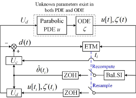
Figure 1: Block diagram of the closed-loop system.

V Main result

The block diagram of the closed-loop system is presented in Figure 1. Before presenting the main result of this paper, we present the following technical lemmas first.

Lemma 1.

For $d(t)$ defined in (42), there exist positive constants ${\epsilon_{1}},{\epsilon_{2}},{\epsilon_{3}},{\epsilon_{4}},{\epsilon_{5}}$ such that

$$\dot{d}(t)^{2}\leq {\epsilon_{1}}d(t)^{2}+{\epsilon_{2}}u(1,t)^{2}+{\epsilon_{3}}u(0,t)^{2}$$

$$+{\epsilon_{4}}\|u(\cdot,t)\|^{2}+{\epsilon_{5}}\zeta(t)^{2}$$ (67)

for $t\in(t_{i},t_{i+1})$, where ${\epsilon_{1}},{\epsilon_{2}},{\epsilon_{3}},{\epsilon_{4}},{\epsilon_{5}}$ only depend on the design parameter $\kappa$ in (23), the known plant parameters, and the known bounds $\overline{a},\underline{a},\overline{\lambda},\underline{\lambda}$ of the unknown parameters.

Proof.

The event-triggered control input $U_{d}$ is constant on $t\in(t_{i},t_{i+1})$, i.e., $\dot{U}_{d}(t)=0$. Taking the time derivative of (42), recalling (1)–(3), we obtain that

$$\dot{d}(t)= \dot{U}_{c}(t)$$

$$= \int_{0}^{1}K_{1}(1,y;\hat{\theta}(t_{i}))u_{t}(y,t)dy+K_{2}(1;\hat{\theta}(t_{i}))\dot{\zeta}(t)$$

$$= \int_{0}^{1}K_{1}(1,y;\hat{\theta}(t_{i}))\varepsilon u_{xx}(y,t)dy$$

$$+\int_{0}^{1}K_{1}(1,y;\hat{\theta}(t_{i}))\lambda u(y,t)dy$$

$$+K_{2}(1;\hat{\theta}(t_{i}))a\zeta(t)+K_{2}(1;\hat{\theta}(t_{i}))bu(0,t)$$

$$= K_{1}(1,1;\hat{\theta}(t_{i}))\varepsilon u_{x}(1,t)-K_{1y}(1,1;\hat{\theta}(t_{i}))\varepsilon u(1,t)$$

$$+K_{1y}(1,0;\hat{\theta}(t_{i}))\varepsilon u(0,t)$$

$$+\int_{0}^{1}K_{1yy}(1,y;\hat{\theta}(t_{i}))\varepsilon u(y,t)dy$$

$$+\int_{0}^{1}K_{1}(1,y;\hat{\theta}(t_{i}))\lambda u(y,t)dy$$

$$+K_{2}(1;\hat{\theta}(t_{i}))a\zeta(t)+K_{2}(1;\hat{\theta}(t_{i}))bu(0,t).$$ (68)

Applying (42), (43), it allows us to rewrite (40) as

$$u_{x}(1,t)+qu(1,t)=U(t)-p(t)-d(t).$$ (69)

Inserting (69) into (68) to replace $u_{x}(1,t)$, we then have

$$\dot{d}(t)= K_{1}(1,1;\hat{\theta}(t_{i}))\varepsilon(-qu(1,t)+U(t)-p(t)-d(t))$$

$$-K_{1y}(1,1;\hat{\theta}(t_{i}))\varepsilon u(1,t)$$

$$+K_{1y}(1,0;\hat{\theta}(t_{i}))\varepsilon u(0,t)$$

$$+\int_{0}^{1}K_{1yy}(1,y;\hat{\theta}(t_{i}))\varepsilon u(y,t)dy$$

$$+\int_{0}^{1}K_{1}(1,y;\hat{\theta}(t_{i}))\lambda u(y,t)dy$$

$$+K_{2}(1;\hat{\theta}(t_{i}))a\zeta(t)+K_{2}(1;\hat{\theta}(t_{i}))bu(0,t)$$

$$= -K_{1}(1,1;\hat{\theta}(t_{i}))\varepsilon d(t)-K_{1}(1,1;\hat{\theta}(t_{i}))\varepsilon p(t)$$

$$-(qK_{1}(1,1;\hat{\theta}(t_{i}))\varepsilon+K_{1y}(1,1;\hat{\theta}(t_{i}))\varepsilon)u(1,t)$$

$$+(K_{1y}(1,0;\hat{\theta}(t_{i}))\varepsilon+K_{2}(1;\hat{\theta}(t_{i}))b)u(0,t)$$

$$+\int_{0}^{1}[K_{1yy}(1,y;\hat{\theta}(t_{i}))\varepsilon+K_{1}(1,y;\hat{\theta}(t_{i}))\lambda$$

$$+K_{1}(1,1;\hat{\theta}(t_{i}))\varepsilon K_{1}(1,y;\theta)]u(y,t)dy$$

$$+(K_{2}(1;\hat{\theta}(t_{i}))a+K_{1}(1,1;\hat{\theta}(t_{i}))\varepsilon K_{2}(1;\theta))\zeta(t),$$ (70)

where (34) has been used.

Applying the Cauchy-Schwarz inequality into (43), we have

$$p(t)^{2}\leq 2\max_{\vartheta_{1},\vartheta_{2}\in\Theta}\left\{\int_{0}^{1}(K_{1}(1,y;\vartheta_{1})-K_{1}(1,y;\vartheta_{2}))^{2}dy\right\}\|u[t]\|^{2}$$

$$+2\max_{\vartheta_{1},\vartheta_{2}\in\Theta}\{(K_{2}(1;\vartheta_{1})-K_{2}(1;\vartheta_{2}))^{2}\}\zeta(t)^{2}.$$ (71)

Applying the Cauchy-Schwarz inequality into (70), using (71), we then obtain (67), where

$${\epsilon_{1}}= 6\varepsilon^{2}\max_{\vartheta\in\Theta}\{K_{1}(1,1;\vartheta)^{2}\},$$ (72)

$${\epsilon_{2}}= 6\max_{\vartheta\in\Theta}\{(qK_{1}(1,1;\vartheta)\varepsilon+K_{1y}(1,1;\vartheta)\varepsilon)^{2}\},$$ (73)

$${\epsilon_{3}}= 6\max_{\vartheta\in\Theta}\{(K_{1y}(1,0;\vartheta)\varepsilon+K_{2}(1;\vartheta)b)^{2}\},$$ (74)

$${\epsilon_{4}}= 12\max_{\vartheta\in\Theta}\left\{\int_{0}^{1}(K_{1yy}(1,y;\vartheta)\varepsilon+K_{1}(1,y;\vartheta)\lambda)^{2}dy\right\}$$

$$+12\varepsilon^{2}\max_{\vartheta\in\Theta}\{K_{1}(1,1;\vartheta)^{2}\}\max_{\vartheta\in\Theta}\left\{\int_{0}^{1}K_{1}(1,y;\vartheta)^{2}dy\right\}$$

$$+12\varepsilon^{2}\max_{\vartheta\in\Theta}\{K_{1}(1,1;\vartheta)^{2}\}$$

$$\quad\times\max_{\vartheta_{1},\vartheta_{2}\in\Theta}\left\{\int_{0}^{1}(K_{1}(1,y;\vartheta_{1})-K_{1}(1,y;\vartheta_{2}))^{2}dy\right\},$$ (75)

$${\epsilon_{5}}= 12{\bar{a}}^{2}\max_{\vartheta\in\Theta}\{(K_{2}(1;\vartheta)^{2}\}$$

$$+12\varepsilon^{2}\max_{\vartheta\in\Theta}\{K_{1}(1,1;\vartheta)^{2}\}\max_{\vartheta\in\Theta}\left\{K_{2}(1;\vartheta)^{2}\right\}$$

$$+12\varepsilon^{2}\max_{\vartheta\in\Theta}\{K_{1}(1,1;\vartheta)^{2}\}$$

$$\quad\times\max_{\vartheta_{1},\vartheta_{2}\in\Theta}\{(K_{2}(1;\vartheta_{1})-K_{2}(1;\vartheta_{2}))^{2}\}.$$ (76)

The proof of Lemma 1 is complete.

Relying on Lemma 1, we present the following lemma which shows that the minimal dwell-time is a positive constant.

Lemma 2.

For some positive $\kappa_{1},\kappa_{2},\kappa_{3},\kappa_{4}$, there exists a minimal dwell-time $\underline{\tau}>0$ such that $t_{i+1}-t_{i}\geq\underline{\tau}$ for all $i\in\mathbb{Z}^{+}$.

Proof.

1) If the event is triggered by the second condition, i.e., $t_{i+1}=t_{i}+T$, in (44), it is obvious that the dwell-time is $T>0$.

2) Next, we consider the case that the event is triggered by the first condition in (44). Define the following function $\psi(t)$:

$$\psi(t)=\frac{{d{{(t)}^{2}}+\frac{1}{2}\xi m(t)}}{{-\frac{1}{2}\xi m(t)}},$$ (77)

which was originally introduced in [13]. We have that $\psi(t_{i+1})=1$ because the event is triggered, and that $\psi(t_{i})<0$ because of $d(t_{i})=0$ according to (42). The function $\psi(t)$ is a continuous function on $[t_{i}^{+},t_{i+1}^{-}]$ recalling Proposition 1 and (42). By the intermediate value theorem, there exists $t^{*}>t_{i}$ such that $\psi(t)\in[0,1]$ when $t\in[t^{*},t_{i+1}^{-}]$. The minimal dwell-time can be founded as the minimal time it takes for $\psi(t)$ from 0 to 1.

Taking the derivative of (77) for all $t\in[t^{*},t_{i+1})$, applying Young’s inequality, using (67) in Lemma 1, and inserting (45), we have

$$\dot{\psi}= \frac{{2d(t)\dot{d}(t)+\frac{1}{2}{\xi}\dot{m}(t)}}{{-\frac{1}{2}\xi m(t)}}-\frac{{\dot{m}(t)}}{{m(t)}}\psi$$

$$\leq \frac{1}{{-\frac{1}{2}\xi m(t)}}\bigg{[}{\epsilon_{1}}d(t)^{2}+{\epsilon_{2}}u(1,t)^{2}+{\epsilon_{3}}u(0,t)^{2}$$

$$+{\epsilon_{4}}\|u(\cdot,t)\|^{2}+{\epsilon_{5}}\zeta(t)^{2}+d{{(t)}^{2}}-\frac{1}{2}{\xi}\eta m(t)$$

$$+\frac{1}{2}{\xi}\lambda_{d}d(t)^{2}-\frac{1}{2}{\xi}{\kappa_{1}}{u}{(1,t)^{2}}-\frac{1}{2}{\xi}{\kappa_{2}}u{(0,t)^{2}}$$

$$-\frac{1}{2}{\xi}{\kappa_{3}}\|{u}{(\cdot,t)\|^{2}}-\frac{1}{2}{\xi}{\kappa_{4}}{\zeta}{(t)^{2}}\bigg{]}-\frac{\lambda_{d}d(t)^{2}}{m(t)}\psi+\eta\psi$$

$$-\frac{-{\kappa_{1}}{u}{(1,t)^{2}}-{\kappa_{2}}u{(0,t)^{2}}-{\kappa_{3}}\|{u}{(\cdot,t)\|^{2}}-{\kappa_{4}}{\zeta}{(t)^{2}}}{m(t)}\psi.$$ (78)

It is worth pointing out that the last term in (78) is less than zero. Choose

$$\kappa_{1} \geq\frac{2{\epsilon_{2}}}{{\xi}},$$ (79)

$$\kappa_{2} \geq\frac{2{\epsilon_{3}}}{{\xi}},$$ (80)

$$\kappa_{3} \geq\frac{2{\epsilon_{4}}}{{\xi}},$$ (81)

$$\kappa_{4} \geq\frac{2{\epsilon_{5}}}{{\xi}},$$ (82)

where ${\epsilon_{2}},{\epsilon_{3}},{\epsilon_{4}},{\epsilon_{5}}$ are given in (73)–(76), which only depend on the design parameter $\kappa$ in (23), the known plant parameters, and the known bounds $\overline{a},\underline{a},\overline{\lambda},\underline{\lambda}$ of the unknown parameters.

Then (78) becomes

$$\dot{\psi}\leq \frac{1}{{-\frac{1}{2}{\xi}m(t)}}\bigg{[}\left({\epsilon_{1}}+1+\frac{1}{2}{\xi}\lambda_{d}\right)d{{(t)}^{2}}-\frac{1}{2}{\xi}\eta m(t)\bigg{]}$$

$$-\frac{\lambda_{d}d(t)^{2}}{m(t)}\psi+\eta\psi.$$ (83)

Inserting

$$\frac{d(t)^{2}}{{m(t)}}= \frac{d(t)^{2}+\frac{1}{2}{\xi}m(t)-\frac{1}{2}{\xi}m(t)}{{m(t)}}$$

$$= -\frac{1}{2}{\xi}\left(\psi(t)+1\right),$$ (84)

we obtain from (83) that

$$\dot{\psi}\leq n_{1}\psi^{2}+n_{2}\psi+n_{3},$$ (85)

where

$$n_{1} =\frac{1}{2}{\lambda_{d}}{\xi},$$ (86)

$$n_{2} =1+{\epsilon_{1}}+{\xi}\lambda_{d}+\eta,$$ (87)

$$n_{3} =1+\eta+{\epsilon_{1}}+\frac{1}{2}{\xi}\lambda_{d}$$ (88)

are positive constants. It follows that the lower bound of dwell-time in this case is

$$\underline{\tau}_{a}=\int_{0}^{1}\frac{1}{n_{1}+n_{2}s+n_{3}s^{2}}ds>0.$$ (89)

Together with the result in 1), we have that the minimal dwell-time $\underline{\tau}$ is

$$\underline{\tau}=\min\{\underline{\tau}_{a},T\}>0.$$ (90)

The proof of this Lemma is complete.

It follows from Lemma 2 that no Zeno phenomenon occurs, i.e., $\lim_{i\to\infty}t_{i}=+\infty$.

Corollary 1.

For all initial data $u[0]\in L^{2}(0,1)$, $\zeta(0)\in\mathbb{R}$, $m(0)\in\mathbb{R}_{-}$, there exist unique mappings $u\in C^{0}(\mathbb{R}_{+};L^{2}(0,1))\bigcap C^{1}(J\times[0,1])$ with $u[t]\in C^{2}([0,1])$, $\zeta\in C^{0}(\mathbb{R}_{+};\mathbb{R})$, $m\in C^{0}(\mathbb{R}_{+};\mathbb{R}_{-})$, which satisfy (2), (3), (40), (66), with (38), (45) for $t>0$, where $J=\mathbb{R}_{+}\backslash\{t_{i}\geq 0,i=0,1,2,\ldots\}$.

Proof.

It is an immediate consequence of Proposition 1 and Lemma 2. Indeed, the solution is constructed (by the step method) iteratively between successive triggering times.

Lemma 3.

The sufficient and necessary conditions of $Q_{n,1}(\mu_{i+1},t_{i+1})=0$, $Q_{n,3}(\mu_{i+1},t_{i+1})=0$ for $n=1,2,\ldots$, are $u[t]=0$, $\zeta(t)=0$ on $t\in[\mu_{i+1},t_{i+1}]$, respectively.

Proof.

Necessity: If $Q_{n,1}(\mu_{i+1},\tau_{i+1})=0$ for $n=1,2,\ldots$, then the definition (61) in conjunction with continuity of $g_{n,1}(t,\mu_{i+1})$ for $t\in[\mu_{i+1},\tau_{i+1}]$ (a consequence of definition (51) and the fact that $u\in C^{0}([\mu_{i+1},\tau_{i+1}];L^{2}(0,1))$) implies

$$g_{n,1}(t,\mu_{i+1})=0,~{}~{}t\in[\mu_{i+1},\tau_{i+1}].$$ (91)

According to the definition (51) and continuity of the mapping $\tau\to\int_{0}^{1}\sin({x\pi n})z[\tau]dx$ (a consequence of the fact that $u\in C^{0}([\mu_{i+1},\tau_{i+1}];L^{2}(0,1))$, (91) implies

$$\int_{0}^{1}\sin({x\pi n})u(x,\tau)dx=0,~{}~{}\tau\in[\mu_{i+1},\tau_{i+1}]$$ (92)

for $n=1,2,\ldots$. Since the set $\{\sqrt{2}\sin(n\pi x):n=1,2,\ldots\}$ is an orthonormal basis of $L^{2}(0,1)$, we have $u[t]=0$ for $t\in[\mu_{i+1},\tau_{i+1}]$.

Sufficiency: If $u[t]=0$ on $t\in[\mu_{i+1},\tau_{i+1}]$, then $Q_{n,1}(\mu_{i+1},\tau_{i+1})=0$ for $n=1,2,\ldots$ is obtained directly, according to (51), (61).

By recalling (52), (63), the fact that the sufficient and necessary condition of $Q_{3n}(\mu_{i+1},t_{i+1})=0$ for $n=1,2,\ldots$ is $\zeta(t)=0$ on $t\in[\mu_{i+1},t_{i+1}]$, is obtained straightforwardly.

The proof of Lemma 3 is complete.

Lemma 4.

For the adaptive estimates defined by (64) based on the data in the interval $t\in[\mu_{i+1},t_{i+1}]$, the following statements hold:

If $u[t]$ (or $\zeta(t)$) is not identically zero for $t\in[\mu_{i+1},t_{i+1}]$, then $\hat{\lambda}(t_{i+1})=\lambda$ (or $\hat{a}(t_{i+1})=a$).

If $u[t]$ (or $\zeta(t)$) is identically zero for $t\in[\mu_{i+1},t_{i+1}]$, then $\hat{\lambda}(t_{i+1})=\hat{\lambda}(t_{i})$ (or $\hat{a}(t_{i+1})=\hat{a}(t_{i})$).

Proof.

First, we define a set as follows,

$$S_{i}:=\bigg{\{}\bar{\ell}=(\ell_{1},\ell_{2})^{T}\in\Theta:Z_{n}(\mu_{i+1},t_{i+1})=G_{n}(\mu_{i+1},t_{i+1})\bar{\ell},$$

$$~{}~{}~{}~{}~{}~{}~{}~{}~{}~{}n=1,2,\ldots,\bigg{\}},~{}~{}i\in\mathbb{Z}^{+},$$ (93)

where ${\Theta=\{\bar{\ell}\in\mathbb{R}^{2}:\underline{\lambda}\leq\ell_{1}\leq\overline{\lambda},\underline{a}\leq\ell_{2}\leq\overline{a}\}}$, and $Z_{n}$, $G_{n}$ in (55), (58) are associated with the plant states over a time interval $[\mu_{i+1},t_{i+1}]$.

We prove the following four claims, from which the statements in this lemma are concluded.

Claim 1.

If $u[t]$ is not identically zero and $\zeta(t)$ is identically zero on $t\in[\mu_{i+1},t_{i+1}]$, then $\hat{\lambda}(t_{i+1})=\lambda$, $\hat{a}(t_{i+1})=\hat{a}(t_{i})$.

Proof.

Because $u[t]$ is not identically zero and $\zeta(t)$ is identically zero on $t\in[\mu_{i+1},\tau_{i+1}]$, there exists $n\in{\mathbb{N}}$ such that $Q_{n,1}(\mu_{i+1},\tau_{i+1})\neq 0$ recalling Lemma 3. Define the index set $I$ to be the set of all $n\in{\mathbb{N}}$ with $Q_{n,1}(\mu_{i+1},\tau_{i+1})\neq 0$. According to (52) and $\zeta(t)$ being identically zero on $t\in[\mu_{i+1},\tau_{i+1}]$, we know that $g_{n,2}(t,\mu_{i+1})=0$ on $t\in[\mu_{i+1},\tau_{i+1}]$ for all $n\in\mathbb{N}$. It follows that $Q_{n,2}(\mu_{i+1},\tau_{i+1})=0$, $Q_{n,3}(\mu_{i+1},\tau_{i+1})=0$, $H_{n,2}(\mu_{i+1},\tau_{i+1})=0$ for all $n\in\mathbb{N}$ recalling (62), (63) and (60). Recalling (55), (58), then (93) implies $S_{i}=\{(\ell_{1},\ell_{2})\in\Theta:\ell_{1}=\frac{H_{n,1}(\mu_{i+1},\tau_{i+1})}{Q_{n,1}(\mu_{i+1},\tau_{i+1})},n\in I\}$. Because $(q_{1},q_{2})\in S_{i}$ according to (54), it follows that $S_{i}=\{(q_{1},\ell_{2})\in\Theta:\underline{a}\leq\ell_{2}\leq\overline{a}\}$. Therefore, (64) shows that $\hat{\lambda}(\tau_{i+1})=\lambda$ and $\hat{a}(\tau_{i+1})=\hat{a}(\tau_{i})$.

Claim 2.

If $u[t]$ is identically zero and $\zeta(t)$ is not identically zero on $t\in[\mu_{i+1},t_{i+1}]$, then $\hat{\lambda}(t_{i+1})=\hat{\lambda}(t_{i})$, $\hat{a}(t_{i+1})=a$.

Proof.

The proof of this claim is very similar to the proof of Claim 1, and thus it is omitted.

Claim 3.

If $u[t]$, $\zeta(t)$ are identically zero on $t\in[\mu_{i+1},t_{i+1}]$, then $\hat{\lambda}(t_{i+1})=\hat{\lambda}(t_{i})$, $\hat{a}(t_{i+1})=\hat{a}(t_{i})$.

Proof.

In this case, $Q_{n,1}(\mu_{i+1},t_{i+1})=0$, $Q_{n,2}(\mu_{i+1},t_{i+1})=0$, $Q_{n,3}(\mu_{i+1},t_{i+1})=0$, $H_{n,1}(\mu_{i+1},t_{i+1})=0$, $H_{n,2}(\mu_{i+1},t_{i+1})=0$ for all $n\in\mathbb{N}$ according to (51), (52), (59)–(63). It follows that $S_{i}=\Theta$, and then (64) shows that $\hat{\lambda}(t_{i+1})=\hat{\lambda}(t_{i})$, $\hat{a}(t_{i+1})=\hat{a}(t_{i})$.

Claim 4.

If both $u[t]$ and $\zeta(t)$ are not identically zero on $t\in[\mu_{i+1},t_{i+1}]$, then $\hat{\lambda}(t_{i+1})=\lambda$, $\hat{a}(t_{i+1})=a$.

Proof.

By virtue of (54), (64), if $S_{i}$ is a singleton then it is nothing else but the least-squares estimate of the unknown vector of parameters $(\lambda,a)$ on the interval $[\mu_{i+1},t_{i+1}]$, and $S_{i}=\{(\lambda,a)\}$. From (55), (58), (93), we have that

$$S_{i}\subseteq S_{ai}:=\bigg{\{}(\ell_{1},\ell_{2})\in\Theta:\ell_{2}=\frac{H_{n,2}(\mu_{i+1},t_{i+1})}{Q_{n,3}(\mu_{i+1},t_{i+1})}$$

$$-\ell_{1}\frac{Q_{n,2}(\mu_{i+1},t_{i+1})}{Q_{n,3}(\mu_{i+1},t_{i+1})},n=1,2,\cdots\bigg{\}}.$$ (94)

We next prove by contradiction that $S_{i}=\{(\lambda,a)\}$. Suppose that on the contrary $S_{i}\neq\{(\lambda,a)\}$, i.e., $S_{i}$ defined by (93) is not a singleton, which implies the set $S_{ai}$ defined by (94) are not singletons (because $S_{ai}$ being a singleton implies that $S_{i}$ is a singleton). It follows that there exist constants $\bar{r}\in\mathbb{R}$ such that

$$\frac{Q_{n,2}(\mu_{i+1},t_{i+1})}{Q_{n,3}(\mu_{i+1},t_{i+1})}=\bar{r},~{}n\in\mathbb{N},$$ (95)

because if there were two different indices $k_{1},k_{2}\in\mathbb{N}$ with $\frac{Q_{k_{1},2}(\mu_{i+1},t_{i+1})}{Q_{k_{1},3}(\mu_{i+1},t_{i+1})}\neq\frac{Q_{k_{2},2}(\mu_{i+1},t_{i+1})}{Q_{k_{2},3}(\mu_{i+1},t_{i+1})}$, then the set $S_{ai}$ defined by (94) would be a singleton.

Moreover, since $S_{i}$ is not a singleton, the definition (93) implies

$$Q_{n,2}(\mu_{i+1},t_{i+1})^{2}=Q_{n,1}(\mu_{i+1},t_{i+1})Q_{n,3}(\mu_{i+1},t_{i+1})$$ (96)

for all $n\in\mathbb{N}$ by recalling (58). According to (61)–(63), and the fact that the Cauchy-Schwarz inequality holds as equality only when two functions are linearly dependent, we obtain the existence of constants $\check{\mu}_{n}$ such that

$$g_{{n},1}(t,\mu_{i+1})=\check{\mu}_{n}g_{{n},2}(t,\mu_{i+1}),~{}~{}n\in\mathbb{N}$$ (97)

for $t\in[\mu_{i+1},t_{i+1}]$ ($g_{{n},2}(t,\mu_{i+1})$ are not identically zero on $t\in[\mu_{i+1},t_{i+1}]$).

Recalling (95), we obtain from (61)–(63) and (97) that

$$g_{n,1}(t,\mu_{i+1}) =\overline{\mu}g_{n,2}(t,\mu_{i+1}),~{}~{}\overline{\mu}\neq 0,~{}~{}n\in\mathbb{N}$$ (98)

for $t\in[\mu_{i+1},t_{i+1}]$. The reason of the constant $\overline{\mu}\neq 0$ is given as follows. According to Lemma 3, there exists $n_{1}\in{\mathbb{N}}$ such that ${Q_{n_{1},1}(\mu_{i+1},t_{i+1})}\neq 0$. Hence, $g_{n_{1},1}(t,\mu_{i+1})$ is not identically zero on $[\mu_{i+1},t_{i+1}]$.

Equations (98) holding is a necessary condition of the hypothesis that $S_{i}$ is not a singleton. Recalling (51), (52), and Proposition 1, the fact that the equation (98) holds implies

$$\int_{0}^{1}\sin({x\pi n})u(x,t)dx+\frac{1}{b}\overline{\mu}\varepsilon\pi n\zeta(t)=0,$$ (99)

for $t\in(\mu_{i+1},t_{i+1})$, $x\in[0,1]$, $n\in\mathbb{N}$.

Taking the time derivative of (99), we have that

$$\int_{0}^{1}\sin({x\pi n})u_{t}(x,t)dx+\frac{1}{b}\overline{\mu}\varepsilon\pi n(a\zeta(t)+bu(0,t))$$

$$= \int_{0}^{1}\sin({x\pi n})(\varepsilon u_{xx}(x,t)+\lambda u(x,t))dx$$

$$+\frac{1}{b}\overline{\mu}\varepsilon\pi n(a\zeta(t)+bu(0,t))$$

$$= -(-1)^{n}\pi n\varepsilon u(1,t)+\pi n\varepsilon u(0,t)$$

$$-\int_{0}^{1}\pi^{2}n^{2}\sin({x\pi n})\varepsilon u(x,t)dx$$

$$+\int_{0}^{1}\sin({x\pi n})\lambda u(x,t)dx$$

$$+\frac{1}{b}\overline{\mu}\varepsilon\pi na\zeta(t)+\overline{\mu}\varepsilon\pi nu(0,t)$$

$$= -(-1)^{n}\pi n\varepsilon u(1,t)+n(\pi\varepsilon+\overline{\mu}\varepsilon\pi)u(0,t)$$

$$-\frac{1}{b}\overline{\mu}\varepsilon\pi n(\lambda-a-\pi^{2}n^{2}\varepsilon)\zeta(t)$$

$$= -(-1)^{n}\pi\varepsilon u(1,t)+(\pi\varepsilon+\overline{\mu}\varepsilon\pi)u(0,t)$$

$$-\frac{1}{b}\overline{\mu}\varepsilon\pi(\lambda-a-\pi^{2}n^{2}\varepsilon)\zeta(t)=0$$ (100)

for $t\in(\mu_{i+1},t_{i+1})$, $n\in\mathbb{N}$, where (99) is applied in going from the second equation to the third one in (100). Considering any two odd (or even) positive integers $n_{1}\neq n_{2}$, we obtain from (100) that $(n_{1}^{2}-n_{2}^{2})\zeta(t)=0$ for $t\in(\mu_{i+1},t_{i+1})$. Considering the fact that $\zeta\in C^{0}([t_{i},t_{i+1}];\mathbb{R})$ and $\zeta(t)$ is not identically zero on $t\in[t_{i},t_{i+1}]$, one obtains $n_{1}^{2}=n_{2}^{2}$: contradiction. Consequently, $S_{i}$ is a singleton, i.e., $S_{i}=\{(\lambda,a)\}$. Therefore, $\hat{\lambda}(t_{i+1})=\lambda,\hat{a}(t_{i+1})=a$.

From Claims 1–4, we obtain Lemma 4.

Lemma 5.

If $\hat{\lambda}(t_{i})=\lambda$ (or $\hat{a}(t_{i})=a$) for certain $i\in\mathbb{Z}^{+}$, then $\hat{\lambda}(t)=\lambda$ (or $\hat{a}(t)=a$) for all $t\in[t_{i},+\infty)$.

Proof.

According to Lemma 4, we have that $\hat{\lambda}(t_{i+1})$ is equal to either $\lambda$ or $\hat{\lambda}(t_{i})$. Therefore, if $\hat{\lambda}(t_{i})=\lambda$, then $\hat{\lambda}(t_{i+1})=\lambda$. Repeating the above process, then $\hat{\lambda}(t)=\lambda$ for all $t\in[t_{i},\lim_{k\to\infty}(t_{k}))$. Recalling Lemma 2 which implies $\lim_{k\to\infty}(t_{k})\to\infty$, we thus have $\hat{\lambda}(t)=\lambda$ for $t\in[t_{i},\infty)$. The same is true of $\hat{a}$. The proof is complete.

Lemma 6.

If $u[0]=0,\zeta(0)\neq 0$, and the user-selected initial estimates $\hat{\lambda}(0),\hat{a}(0)$ happen to make $K_{2}(1;\hat{\theta}(0))=K_{2}(1;\hat{\lambda}(0),\hat{a}(0))=0$, the constant $K_{2}(1;\hat{\theta}(t_{1}))\neq 0$ is ensured just by changing $\hat{\lambda}(0)$ as another value (arbitrary) in $[\underline{\lambda},\overline{\lambda}]$.

Proof.

Because the kernels $h$ and $\gamma$ in $K_{2}$ (36) only include the unknown parameter: $a$, considering $\hat{a}(t_{1})=a$ ensured by $\zeta(0)\neq 0$ with Lemma 4, and $\hat{\lambda}(t_{1})=\hat{\lambda}(0)$ due to the fact that $u[t]$ is identically zero on $t\in[0,t_{1}]$ (which is the result of $K_{2}(1;\hat{\theta}(0))=0$ with (1)–(3), (38), (40) and $u[0]=0$), we have that

$$K_{2}(1;\hat{\theta}(t_{1})) =K_{2}(1;\hat{\lambda}(t_{1}),\hat{a}(t_{1}))=K_{2}(1;\hat{\lambda}(0),a)$$

$$=K_{2}(1;\theta)+\frac{\lambda-\hat{\lambda}(0)}{2\varepsilon}\gamma(1).$$ (101)

If $K_{2}(1;\hat{\theta}(t_{1}))=0$, it implies that

$$\hat{\lambda}(0)=\lambda+\frac{2\varepsilon K_{2}(1;\theta)}{\gamma(1)}.$$ (102)

Therefore, once we pick another $\hat{\lambda}(0)$, then $K_{2}(1;\hat{\theta}(t_{1}))\neq 0$ is ensured in the situation mentioned in this lemma.

The proof of Lemma 6 is complete.

Remark 1.

If $u[0]=0,\zeta(0)\neq 0$, and $K_{2}(1;\hat{\theta}(0))=0$ is found under the user-selected initial estimates $\hat{\theta}(0)=[\hat{\lambda}(0),\hat{a}(0)]^{T}$, then $\hat{\lambda}(0)$ should be changed as another value (arbitrary) in $[\underline{\lambda},\overline{\lambda}]$.

According to Lemma 6, the purpose of Remark 1 is to avoid the appearance of an extreme case that $u[0]=0$, $\zeta(0)\neq 0$, $K_{2}(1;\hat{\theta}(0))=0$, $K_{2}(1;\hat{\theta}(t_{1}))=0$, which implies $K_{2}(1;\hat{\theta}(t))=K_{2}(1;\hat{\theta}(t_{1}))=K_{2}(1;\hat{\lambda}(0),a)=0$ for $t\geq t_{1}$, and leads to that the regulation on the ODE dynamics (1) is lost, i.e., $u[t]\equiv 0$ for all time while $\zeta(t)$ dynamics may be unstable, according to (1)–(3), (38), (40).

Let $\hat{\theta}(0)$ belong to $\Theta_{1}$ which is equal to $\Theta$ under Remark 1, we obtain the following parameter convergence property.

Lemma 7.

For $\hat{\theta}(0)\in\Theta_{1}$, and all $u[0]\in L^{2}(0,1)$, $\zeta(0)\in\mathbb{R}$ except for the case that both $u[0]$ and $\zeta(0)$ are zero, we have

$$\hat{\lambda}(t)=\lambda,~{}~{}~{}~{}\hat{a}(t)=a$$ (103)

for all $t\geq t_{2}$.

Proof.

Case 1: $u(x,0)$ is not identically zero for $x\in[0,1]$, and $\zeta(0)$ is not zero. We know that $u[t],\zeta(t)$ are not identically zero on $t\in[0,t_{1}]$. Recalling Lemmas 4, 5, we obtain (103).

Case 2: $u[0]=0$ and $\zeta(0)\neq 0$.

We know that $\zeta(t)$ is not identically zero on $t\in[0,t_{1}]$. If $K_{2}(1;\hat{\lambda}(0),\hat{a}(0))\neq 0$, we have that $u[t]$ is not identically zero on $t\in[0,t_{1}]$ according to (1)–(3), (38), (40). Then it is straightforward to obtain (103) with recalling Lemmas 4, 5.

If $K_{2}(1;\hat{\lambda}(0),\hat{a}(0))=0$, then $u[t]=0$ on $t\in[0,t_{1}]$ according to (1)–(3), (38), (40) and $u[0]=0$. It follows that $\zeta(t)=\zeta(0)e^{at}$ in (1), which is not zero on $t\in[0,t_{1}]$ under $\zeta(0)\neq 0$. Recalling Lemma 6 and Remark 1, we have $K_{2}(1;\hat{\theta}(t_{1}))\neq 0$, which results in that $u[t]$ is not identically zero on $t\in[t_{1},t_{2}]$ considering (1)–(3), (38), (40), and the fact that $\zeta(t_{1})=\zeta(0)e^{at_{1}}$ is not zero. Therefore, we obtain (103) from Lemmas 4, 5.

Case 3: $u(x,0)$ is not identically zero, and $\zeta(0)=0$.

It is obvious that $u[t]$ is not identically zero on $t\in[0,t_{1}]$. Supposing that $\zeta[t]$ is identically zero on $t\in[0,t_{1}]$, it follows from (1) that $u(0,t)=0$ on $t\in[0,t_{1}]$. Applying the method of separation of variables shown in (3.4)–(3.10) in [31], it implies from (2), (3) and $u(0,t)=0$ that $u[t]$ is identically zero on $t\in[0,t_{1}]$: contradiction. Therefore, $\zeta[t]$ is also not identically zero on $t\in[0,t_{1}]$. We thus obtain (103) from Lemmas 4, 5.

The proof of this lemma is complete.

We are now ready to show the main result of this paper.

Theorem 1.

For all initial data $u[0]\in L^{2}(0,1)$, $\zeta(0)\in\mathbb{R}$, $m(0)\in\mathbb{R}_{-}$, and $\hat{\theta}(0)\in\Theta_{1}$, the closed-loop system, i.e., (1)–(4) under the controller (38), with the event-triggering mechanism (44), (45), and the least-squares identifier defined by (64), has the following properties:

1) Except for the case that both $u[0]$ and $\zeta(0)$ are zero, there exist positive constants $M,\sigma$ (independent of initial conditions) such that

$$\Omega(t)\leq M\Omega(0)e^{-\sigma t},~{}~{}t\in[0,\infty)$$ (104)

where

$$\Omega(t)=\|u[t]\|^{2}+\zeta(t)^{2}+|m(t)|+\left|\tilde{\theta}(t)\right|.$$ (105)

The signal bars $|\cdot|$ for $\tilde{\theta}(t)=\theta-\hat{\theta}(t)$ denotes the Euclidean norm.

2) If both $u[0]$ and $\zeta(0)$ are zero, all signals are bounded in the sense of

$$\Omega(t)\leq|m(0)|+\left|\theta-\hat{\theta}(0)\right|,~{}~{}t\in[0,\infty).$$ (106)

Proof.

1) Now we prove the first of the two portions of the theorem.

Define a Lyapunov function as

$$V(t)=\frac{1}{2}r_{a}\int_{0}^{1}\beta(x,t)^{2}dx+\frac{1}{2}r_{c}\zeta(t)^{2}-m(t)$$ (107)

where $m(t)$ is defined in (45).

Defining

$$\bar{\Omega}(t)=\|\beta[t]\|^{2}+\zeta(t)^{2}+|m(t)|,$$ (108)

we have

$$\xi_{3}\bar{\Omega}(t)\leq V(t)\leq\xi_{4}\bar{\Omega}(t)$$ (109)

where

$$\xi_{3}= \min\left\{\frac{1}{2}r_{a},\frac{1}{2}r_{c},1\right\}>0,$$

$$\xi_{4}= \max\left\{\frac{1}{2}r_{a},\frac{1}{2}r_{c},1\right\}>0.$$ (110)

According to (69) and the nominal control design in Section III, in the triggered control system, the right boundary condition of the target system (25)–(28) becomes

$$\beta_{x}(1,t)+r\beta(1,t)=-p(t)-d(t).$$ (111)

For $t\in(t_{i},t_{i+1})$, $i\in\mathbb{Z}^{+}$, taking the derivative of (107) along (25)–(27), (111), recalling (45), we have that

$$\dot{V}(t)= r_{a}\int_{0}^{1}\beta(x,t)\beta_{t}(x,t)dx+r_{c}\zeta(t)\dot{\zeta}(t)-\dot{m}(t)$$

$$+r_{a}\int_{0}^{1}\beta(x,t)\varepsilon\beta_{xx}(x,t)dx+r_{c}\zeta(t)\dot{\zeta}(t)-\dot{m}(t)$$

$$= r_{a}\varepsilon\beta(1,t)\beta_{x}(1,t)-r_{a}\varepsilon\beta(0,t)\beta_{x}(0,t)$$

$$-r_{a}\varepsilon\int_{0}^{1}\beta_{x}(x,t)^{2}dx-r_{c}a_{\rm m}\zeta(t)^{2}$$

$$+r_{c}\zeta(t)b\beta(0,t)+\eta m(t)-\lambda_{d}d(t)^{2}$$

$$+{\kappa_{1}}{\beta}{(1,t)^{2}}+{\kappa_{2}}{\beta(0,t)^{2}}+{\kappa_{3}}\|u(\cdot,t)\|^{2}+{\kappa_{4}}\zeta(t)^{2}$$

$$= r_{a}\varepsilon\beta(1,t)(-r\beta(1,t)-p(t)-d(t))$$

$$-r_{a}\varepsilon\int_{0}^{1}\beta_{x}(x,t)^{2}dx-a_{\rm m}r_{c}\zeta(t)^{2}+r_{c}\zeta(t)b\beta(0,t)$$

$$+\eta m(t)-\lambda_{d}d(t)^{2}+{\kappa_{1}}{u}{(1,t)^{2}}+{\kappa_{2}}{u(0,t)^{2}}$$

$$+{\kappa_{3}}\|u(\cdot,t)\|^{2}+{\kappa_{4}}\zeta(t)^{2}.$$ (112)

Recalling (14), (16), (37), we have

$$u(x,t)$$

$$= \beta(x,t)-\int_{0}^{x}h^{I}(x,y)\beta(y,t)dy+\gamma(x)\zeta(t)$$

$$-\int_{0}^{x}{\Phi}(x,y)\left(\beta(y,t)-\int_{0}^{y}h^{I}(y,z)\beta(z,t)dz+\gamma(y)\zeta(t)\right)dy$$

$$= \beta(x,t)+\int_{0}^{x}P(x,y)\beta(y,t)dy+\Gamma(x)\zeta(t)$$ (113)

where

$$P(x,y) =\int_{y}^{x}{\Phi}(x,z)h(z,y)dz-h(x,y)-{\Phi}(x,y),$$ (114)

$$\Gamma(x) =\gamma(x)-\int_{0}^{x}{\Phi}(x,y)\gamma(y)dy.$$ (115)

Applying the Cauchy-Schwarz inequality, we obtain

$$u(0,t)^{2} \leq m_{1}(\beta(0,t)^{2}+\zeta(t)^{2}),$$ (116)

$$u(1,t)^{2} \leq m_{2}(\beta(1,t)^{2}+\zeta(t)^{2}+\|\beta[t]\|^{2}),$$ (117)

$$\|u[t]\|^{2} \leq m_{3}(\zeta(t)^{2}+\|\beta[t]\|^{2}),$$ (118)

where

$$m_{1}= 2\max\{1,\max_{\vartheta\in\Theta}\{\Gamma(0;\vartheta)^{2}\}>0,$$

$$m_{2}= 3\max_{\vartheta\in\Theta}\bigg{\{}1,\int_{0}^{1}P(1,y;\vartheta)^{2}dy,\Gamma(1;\vartheta)^{2}\bigg{\}}>0,$$

$$m_{3}= 2\max_{\vartheta\in\Theta}\bigg{\{}\left(1+\left(\int_{0}^{1}\int_{0}^{x}P(x,y;\vartheta)^{2}dydx\right)^{\frac{1}{2}}\right)^{2},$$

$$\int_{0}^{1}\Gamma(x;\vartheta)^{2}dx\bigg{\}}>0.$$ (119)

From Poincare inequality, we have that

$$-\|\beta_{x}[t]\|^{2}\leq\frac{1}{2}\beta(1,t)^{2}-\frac{1}{4}\|\beta[t]\|^{2}.$$ (120)

From Agmon’s and Young’s inequalities, we have that

$$\beta(0,t)^{2}\leq\beta(1,t)^{2}+\|\beta[t]\|^{2}+\|\beta_{x}[t]\|^{2}.$$ (121)

Applying Young’s inequality and the Cauchy-Schwarz inequality into (112), with using (116)–(118), (120), (121), we have that

$$\dot{V}(t)\leq -rr_{a}\varepsilon\beta(1,t)^{2}-r_{a}\varepsilon\beta(1,t)p(t)-r_{a}\varepsilon\beta(1,t)d(t)$$

$$-\frac{1}{8}r_{a}\varepsilon\int_{0}^{1}\beta(x,t)^{2}dx+\frac{1}{4}r_{a}\varepsilon\beta(1,t)^{2}$$

$$-\frac{1}{2}r_{a}\varepsilon\int_{0}^{1}\beta_{x}(x,t)^{2}dx-\frac{3}{4}a_{\rm m}r_{c}\zeta(t)^{2}+\frac{r_{c}}{a_{\rm m}}b^{2}\beta(0,t)^{2}$$

$$+\eta m(t)-\lambda_{d}d(t)^{2}+{\kappa_{1}m_{2}}{\beta}{(1,t)^{2}}+{\kappa_{2}}m_{1}{\beta(0,t)^{2}}$$

$$+({\kappa_{3}}m_{3}+{\kappa_{1}}m_{2})\|\beta(\cdot,t)\|^{2}$$

$$+({\kappa_{4}}+{\kappa_{2}}m_{1}+{\kappa_{1}m_{2}}+{\kappa_{3}}m_{3})\zeta(t)^{2}$$

$$\leq -\bigg{[}\left(r-\frac{1}{4}\right)r_{a}\varepsilon-\frac{r_{a}\varepsilon}{4r_{1}}-\frac{r_{a}\varepsilon}{4r_{2}}-\frac{r_{c}}{a_{\rm m}}b^{2}$$

$$-{\kappa_{1}}m_{2}-\kappa_{2}m_{1}\bigg{]}\beta(1,t)^{2}$$

$$+\eta m(t)-(\lambda_{d}-r_{1}r_{a}\varepsilon)d(t)^{2}+r_{2}r_{a}\varepsilon p(t)^{2}$$

$$-\left(\frac{3r_{c}}{4}a_{\rm m}-{\kappa_{1}m_{2}}-{\kappa_{2}}m_{1}-{\kappa_{3}}m_{3}-{\kappa_{4}}\right)\zeta(t)^{2}$$

$$-\left(\frac{1}{2}r_{a}\varepsilon-\frac{r_{c}}{a_{\rm m}}b^{2}-{\kappa_{2}}m_{1}\right)\|\beta_{x}[t]\|^{2}$$

$$-\left(\frac{1}{8}r_{a}\varepsilon-\frac{r_{c}}{a_{\rm m}}b^{2}-{\kappa_{1}}m_{2}-{\kappa_{2}}m_{1}-{\kappa_{3}}m_{3}\right)\|\beta[t]\|^{2}$$ (122)

for $t\in(t_{i},t_{i+1})$. Choosing

$$\min\{r_{1},r_{2}\}\geq \frac{1}{q-\frac{\overline{\lambda}}{2\varepsilon}-\frac{1}{4}}\geq\frac{1}{r-\frac{1}{4}},$$ (123)

$$r_{c}> \frac{8({\kappa_{1}m_{2}}+{\kappa_{2}}m_{1}+{\kappa_{3}}m_{3}+{\kappa_{4}})}{3a_{\rm m}},$$ (124)

$$r_{a}\geq \max\bigg{\{}\frac{2(\frac{r_{c}}{a_{m}}b^{2}+{\kappa_{1}}m_{2}+{\kappa_{2}}m_{1})}{{(q-\frac{\overline{\lambda}}{2\varepsilon}-\frac{1}{4})}\varepsilon},$$

$$\frac{2}{\varepsilon}\left(\frac{r_{c}}{a_{\rm m}}b^{2}+{\kappa_{2}}m_{1}\right),$$

$$\frac{16(\frac{r_{c}}{a_{\rm m}}b^{2}+{\kappa_{1}}m_{2}+{\kappa_{2}}m_{1}+{\kappa_{3}}m_{3})}{\varepsilon}\bigg{\}},$$ (125)

$$\lambda_{d}\geq r_{1}r_{a}\varepsilon,$$ (126)

where $r=q-\frac{\lambda}{2\varepsilon}$ in (29) and Assumption 2 which ensure $r\geq q-\frac{\overline{\lambda}}{2\varepsilon}>\frac{1}{4}$ are recalled, we obtain

$$\dot{V} \leq-\frac{1}{16}r_{a}\varepsilon\|\beta[t]\|^{2}-\frac{3r_{c}}{8}a_{\rm m}\zeta(t)^{2}$$

$$\quad+\eta m(t)+r_{2}r_{a}\varepsilon p(t)^{2}.$$ (127)

That is,

$$\dot{V}\leq-\sigma V(t)+r_{2}r_{a}\varepsilon p(t)^{2}$$ (128)

for $t\in(t_{i},t_{i+1})$, $i\in\mathbb{Z}^{+}$, where

$$\sigma=\min\left\{\frac{1}{8}\varepsilon,\frac{3}{4}a_{\rm m},\eta\right\}.$$ (129)

Claim 5.

After $t=t_{2}$, $p(t)$ defined in (43) is identically zero, i.e.,

$$p(t)\equiv 0,~{}~{}t\in[t_{2},\infty).$$ (130)

Proof.

1) If $u[0]$ and $\zeta(0)$ are zero, it follows that $u[t]$ and $\zeta(t)$ are identically zero for $t\in[0,\infty)$ considering (1)–(3), (38), (40). Thus (130) holds.

2) Others: Recalling (43) and Lemma 7, we obtain (130).

The proof of Claim 5 is complete.

Multiplying both sides of (128) by $e^{\sigma t}$, integrating both sides of (128) from $t_{i}$ to $t_{i+1}$, $i\geq 2$, considering Claim 5, we obtain that

$$V(t)\leq V(t_{i})e^{-\sigma(t-t_{i})},~{}~{}t\in(t_{i},t_{i+1}),~{}~{}i\geq 2.$$ (131)

Recalling Corollary 1, we know that $V(t)$ defined in (107) is continuous. We then have $V(t_{i+1}^{-})=V(t_{i+1})$ and $V(t_{i}^{+})=V(t_{i})$, and thus we can replace $(t_{i},t_{i+1})$ by $[t_{i},t_{i+1}]$ in (131), yielding

$$V(t_{i+1})\leq V(t_{i})e^{-\sigma(t_{i+1}-t_{i})},$$ (132)

for $i\geq 2$.

Hence, applying (132) repeatedly, we obtain from (131) that

$$V(t)\leq V(t_{2})\prod_{c=2}^{i-1}e^{-\sigma(t_{c+1}-t_{c})}e^{-\sigma(t-t_{i})}$$

$$= V(t_{2})e^{-\sigma(t-t_{2})}$$ (133)

for any $t\in[t_{i},t_{i+1}],i\geq 3$. Together with (131) holding for $t\in[t_{2},t_{3}]$, we obtain

$$V(t)\leq V(t_{2})e^{-\sigma(t-t_{2})}$$ (134)

for $t\geq t_{2}$.

In the following claim, we analyze the responses on $t\in[0,t_{2}]$.

Claim 6.

For the finite time $t_{2}$ in Claim 5, the following estimate holds,

$$V(t)\leq V(0)e^{\bar{\sigma}t},~{}~{}t\in[0,t_{2}]$$ (135)

where

$$\bar{\sigma}= \frac{1}{\xi_{3}}\max\{r_{2}r_{a}\varepsilon\Upsilon_{p},1\}$$

$$-\min\left\{\frac{1}{8}\varepsilon,\frac{3}{4}a_{\rm m},\eta+1\right\}$$ (136)

for some positive $\Upsilon_{p}$.

Proof.

Bounding $p(t)^{2}$ defined in (43) on $t\in[0,t_{2}]$ as

$$p(t)^{2}\leq\bar{\Upsilon}_{p}(\|u[t]\|^{2}+\zeta(t)^{2}).$$ (137)

where

$$\bar{\Upsilon}_{p}= 2\max\bigg{\{}\max_{\vartheta\in\Theta}\left\{\int_{0}^{1}(K_{1}(1,y;\theta)-K_{1}(1,y;\vartheta))^{2}dy\right\},$$

$$\max_{\vartheta\in\Theta}\{(K_{2}(1;\theta)-K_{2}(1;\vartheta))^{2}\}\bigg{\}}.$$ (138)

Recalling (118), we obtain

$$p(t)^{2}\leq\Upsilon_{p}(\|\beta[t]\|^{2}+\zeta(t)^{2}),~{}~{}t\in[0,t_{2}]$$ (139)

where the positive constant $\Upsilon_{p}$ is

$$\Upsilon_{p}=\max\left\{\bar{\Upsilon}_{p}m_{3},\bar{\Upsilon}_{p}(m_{3}+1)\right\}.$$ (140)

For $0\leq i<2$, we have from (127) and (139) that

$$\dot{V}(t) \leq-\frac{1}{16}r_{a}\varepsilon\|\beta[t]\|^{2}-\frac{3r_{c}}{8}a_{\rm m}\zeta(t)^{2}+\eta m(t)+m(t)$$

$$\quad-m(t)+r_{2}r_{a}\varepsilon\Upsilon_{p}(\|\beta[t]\|^{2}+\zeta(t)^{2})$$

$$\leq\bar{\sigma}V(t),~{}~{}~{}t\in(t_{i},t_{i+1})$$ (141)

where $\bar{\sigma}$ is given in (136).

We then have

$$V(t)\leq V(t_{i})e^{\bar{\sigma}(t-t_{i})},$$ (142)

for $t\in(t_{i},t_{i+1}),0\leq i<2$. Recalling again the continuity of $V(t)$, and thus we can replace $(t_{i},t_{i+1})$ by $[t_{i},t_{i+1}]$ in (142).

Then we have

$$V(t_{1})\leq V(0)e^{\bar{\sigma}t_{1}}.$$ (143)

Recalling (142) and applying (143), we have that

$$V(t) \leq V(0)e^{{\bar{\sigma}}t_{1}}e^{{\bar{\sigma}}(t-t_{1})}$$

$$=V(0)e^{{\bar{\sigma}}t}$$ (144)

for any $t\in[t_{1},t_{2}]$. It is obtained from (142) that $V(t)\leq V(0)e^{{\bar{\sigma}}t}$ also holds for $t\in[0,t_{1}]$. Therefore, (135) holds.

The proof of Claim 6 is complete.

We obtain from Claim 6 that

$$V(t_{2})\leq V(0)e^{{\bar{\sigma}}t_{2}}.$$ (145)

By virtue of (134), (135), (145), we have

$$V(t)\leq V(0)e^{(\bar{\sigma}+{\max\{\sigma,-\bar{\sigma}\})t_{2}}}e^{-\sigma t}$$

$$\leq V(0)e^{2T(\bar{\sigma}+{\max\{\sigma,-\bar{\sigma}\})}}e^{-\sigma t}$$ (146)

for $t\in[0,\infty)$, where

$$t_{2}\leq 2T$$ (147)

ensured by (44) is recalled.

Recalling (109), we have

$$\bar{\Omega}(t)\leq\Upsilon_{1}\bar{\Omega}(0)e^{-\sigma t},t\geq 0$$ (148)

where the positive constant $\Upsilon_{1}$ is

$$\Upsilon_{1}=\frac{\xi_{4}}{\xi_{3}}e^{2T(\bar{\sigma}+{\max\{\sigma,-\bar{\sigma}\})}}.$$ (149)

From (II), (39) and Lemma 7, we know that

$$\tilde{\theta}(t)=0,~{}~{}~{}\forall t\geq t_{2},$$ (150)

and

$$\left|\tilde{\theta}(t)\right|\leq\left|\tilde{\theta}(0)\right|,~{}~{}~{}\forall t\in[0,t_{2}],$$ (151)

which is ensured by Lemma 4.

Recalling (147), the following estimate holds

$$\left|\tilde{\theta}(t)\right|\leq e^{2\sigma T}\left|\tilde{\theta}(0)\right|e^{-\sigma t}.$$ (152)

Therefore, together with (148), we have that

$$\left(\bar{\Omega}(t)+\left|\tilde{\theta}(t)\right|\right)\leq\Upsilon\left(\bar{\Omega}(0)+\left|\tilde{\theta}(0)\right|\right)e^{-\sigma t}$$ (153)

where

$$\Upsilon=\max\{\Upsilon_{1},e^{2\sigma T}\}.$$ (154)

Applying the invertibility of the transformations (8), (16), (24), we thus obtain (104).

2) Now we prove the second of the two portions of the theorem. It follows from (1)–(3), (38), (40) and $u[0]=0$, $\zeta(0)=0$ that $u[t]\equiv 0$ and $\zeta(t)\equiv 0$ for $t\in[0,\infty)$. Recalling (42), (45), we know $m(t)=m(0)e^{-\eta t}$, i.e., $|m(t)|\leq|m(0)|$, for $t\in[0,\infty)$. Also, it is obtained (by the step method) from Lemma 4 that $\hat{\theta}(t)\equiv\hat{\theta}(0)$ for $t\in[0,\infty)$, i.e., $\tilde{\theta}(t)\equiv\theta-\hat{\theta}(0)$ for $t\in[0,\infty)$. Therefore, (106) is obtained.

The proof of the theorem is complete.

In the proposed control system, all conditions of the design parameters are cascaded rather than coupled, and only depend on the known parameters. An order of selecting the design parameters is shown in Figure 2.

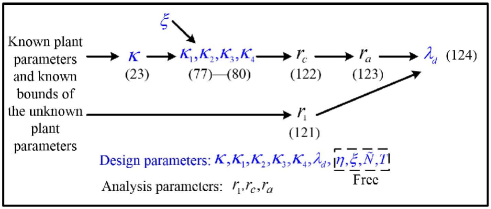
Figure 2: An order of selecting the design parameters.

VI Simulation

VI-A Model

The simulation model is (1)–(4) with the following parameters

$$a=1.5,~{}b=1,~{}\varepsilon=1,~{}\lambda=3,~{}q=5.$$

The bounds $\overline{\lambda},\underline{\lambda},\overline{a},\underline{a}$ of the unknown parameters $\lambda$, $a$ are set as $0,5,0,3$, respectively. Initial conditions are defined as

$$u(x,0)=x^{2}\sin(2\pi x),~{}~{}\zeta(0)=5.$$ (155)

In the numerical calculation by the finite difference method, the model is discretized with the time step of $0.004$ and the space step of $0.05$.

VI-B Design Parameters

The design parameters are chosen as $\xi=1.1$, $\tilde{N}=5$, $T=1.2$, $\eta=15$, $\kappa=16$, $\kappa_{1}=\kappa_{2}=\kappa_{3}=\kappa_{4}=100$, $\lambda_{d}=20$, and $n$ in (64) is truncated at $15$ and the initial condition of $m(t)$ is set as $m(0)=-500$. The function of free design parameters $\tilde{N}$, $T$, $\eta$, $\xi$ and $m(0)$ in adjusting the response of the closed-loop system is illustrated as follows. A larger $m(0)$ can reduce the triggering times at the initial stage, which allows more data being collected for least-squares parameter identification. Even though a larger overshoot of the plant norms may appear due to the large $m(0)$, the increase of $\eta$ can fasten the convergence of $m(t)$ to zero, together with the decrease of $\xi$, which can make the plant states resampled more frequently, especially after the parameter estimates reaching the true values (which can always be achieved in initial several updates), and thus increase the decay rate of the plant states. Besides, as mentioned when introduce the design parameters $\tilde{N},T$, the increase of $\tilde{N}$ allows the data in more time intervals to be used in parameter identification, which can improve the accuracy and robustness of the identifier, and $T$ is chosen to avoid less frequent updates of parameter estimates considering the operation time is only $4$ s.

VI-C Gain Kernels

The kernels $\lambda(x)$, ${\Psi}(x,y)$ are directly obtained from (17), (9) (using the modified Bessel function given in (A.10) in [31] with $n=1$ and cutting off $m$ in (A.10) at 15), where the unknown coefficients are replaced by the piecewise-constant estimates. The approximate solution $h(x,y)$ of (30)–(33) where the unknown coefficients are replaced by the piecewise-constant estimates is obtained by the finite difference method on a lower triangular domain discretized as a grid with the uniformed interval of $0.05$ (the spatial variables $x$ and $y$ were discretized using 21 grid points each). The value at each grid point is denoted as $h_{i,j}$, $1\leq j\leq i\leq 21$, $i,j\in\mathbb{N}$. According to (33), we know $h_{1,1}=0$. Together with (32), we have $h_{i,i}=0$, $i=1,2,\cdots,21$. Then $h_{2,1}$ can be solved via (30). For representing the two-order derivatives in (31) by the finite difference scheme, we adopt the following approximate $h_{i,i-1}=h_{2,1},i=2,\cdots,21$. The kernel $h$ will be recomputed when the parameter estimates are changed in the evolution. In the simulation results which will be shown later, we know that $h$ is recomputed twice, according to the parameter estimates $\hat{\lambda}$ and $\hat{a}$.

VI-D Simulation Results

The open-loop response of the ODE state $\zeta(t)$ and PDE state $u(x,t)$ are shown in Figures 3, 4, from which we observe that the plant is unstable. Applying the proposed adaptive event-triggered controller $U_{d}$ defined in (38), it is shown in Figures 5, 6 that the ODE state $\zeta(t)$ and PDE state $u(x,t)$ are convergent to zero. The piecewise-constant control input $U_{d}(t)$ defined in (38) and the continuous-in-state control signal $U_{c}(t)$ (41) used in ETM are shown in Figure 7. For the control input $U_{d}(t)$, the estimate $\hat{\theta}$ is recomputed and the states $u$, $\zeta$ are resampled simultaneously, the total number of triggering times is $26$, the minimal dwell-time is $0.0404$ s, which is much larger than the highly conservative minimal dwell time estimate (whose order of magnitude is $10^{-6}$ s) obtained from (89), (90) in Lemma 2. There are two ”jumps” in the continuous-in-state control signal $U_{c}(t)$ (41) at the first two triggering times, because of the updates in the parameter estimates which are shown in Figure 8, where the estimates reach the true values after two triggering times (the exact estimates are not obtained at the time of the first event under the nonzero initial condition (155) as Lemmas 4, 5 imply, because of the approximation adopted in the simulation, including the discretization of time and space, and truncation of $n=1,2,\cdots$ in the estimator (64)).

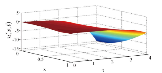
Figure 3: The evolution of $u(x,t)$ in open loop.

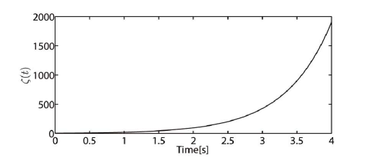
Figure 4: The evolution of $\zeta(t)$ in open loop.

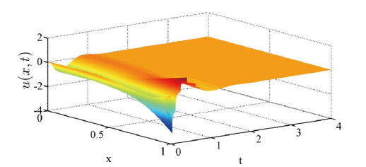
Figure 5: The evolution of $u(x,t)$ under the control input $U_{d}(t)$ defined in (38).

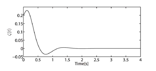
Figure 6: The evolution of $\zeta(t)$ under the control input $U_{d}(t)$ defined in (38).

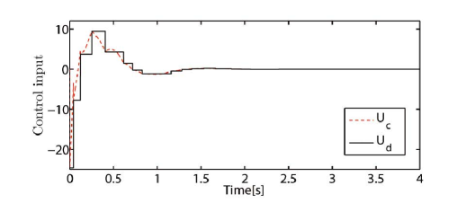
Figure 7: The piecewise-constant control input $U_{d}(t)$ (38) and the continuous-in-state control signal $U_{c}(t)$ (41) used in ETM.

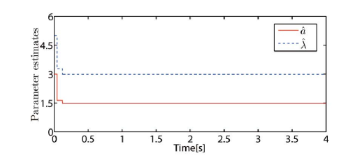
Figure 8: The evolution of the parameter estimates.

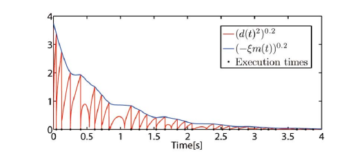
Figure 9: The evolution of $(d(t)^{2})^{0.2}$ and $(-\xi m(t))^{0.2}$.

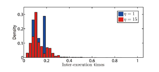
Figure 10: Density of the inter-execution times computed for 100 different initial conditions given by $u(x,0)=x^{2}\sin(\bar{n}\pi x)$, $\zeta(0)=0.2$, $\bar{n}=1,2,\ldots,100$.

Figure 9 shows the time evolution of the functions in the triggering condition (44) and the execution times, where an event is generated, the control value is updated and $d(t)$ is reset to zero, when the trajectory $d(t)^{2}$ reaches the trajectory $-\xi m(t)$.

Finally, we run simulations for 100 different initial conditions and compute the inter-execution times between two triggering times. The density of the inter-execution times is shown in Figure 10, from which we know that the prominent inter-execution times are around $0.1$ s when $\eta=15$, and increase to around 0.2 s when $\eta$ decreases to 1.

VII Conclusion and future work

In this paper, we have proposed an adaptive event-triggered boundary control scheme for a parabolic PDE-ODE system, where the reaction coefficient of the parabolic PDE, and the system parameter of the ODE are unknown, and both of the parameter estimates and control input employ piecewise-constant values. The controller includes an event-triggering mechanism to determine the synchronous update times of both the batch least-squares identifier and plant states in the control law. We have proved that the proposed control guarantees: 1) no Zeno phenomenon occurs; 2) parameter estimates are convergent to the true values in finite time under most initial conditions of the plant (all initial conditions except a set of measure zero); 3) the plant states are exponentially regulated to zero. The effectiveness of the proposed design is verified by a numerical example. In the future work, the state-feedback control design will be extended to the output-feedback type conforming to available sensors in practice.

Appendix

VII-A Calculating Conditions of $\gamma(x)$

Inserting (16) into (18), recalling (10), (22), we have

$$\dot{\zeta}(t)+a_{\rm m}\zeta(t)-{b}w(0,t)+b\gamma(0)\zeta(t)$$

$$= \dot{\zeta}(t)-a\zeta(t)-{b}w(0,t)+(b\kappa+b\gamma(0))\zeta(t)$$

$$= (b\kappa+b\gamma(0))\zeta(t)=0.$$ (A.1)

Inserting (16) into (19), recalling (11), (18), we have

$${v_{t}}(x,t)-{\varepsilon}{v_{xx}}(x,t)+\gamma(x){b}v(0,t)$$

$$= w_{t}(x,t)-\gamma(x)\dot{\zeta}(t)-{\varepsilon}w_{xx}(x,t)$$

$$+{\varepsilon}\gamma^{\prime\prime}(x)\zeta(t)+\gamma(x){b}v(0,t)$$

$$= \gamma(x)a_{\rm m}\zeta(t)-\gamma(x){b}v(0,t)+{\varepsilon}\gamma^{\prime\prime}(x)\zeta(t)+\gamma(x){b}v(0,t)$$

$$= (\gamma(x)a_{\rm m}+{\varepsilon}\gamma^{\prime\prime}(x))\zeta(t)=0.$$ (A.2)

By virtue of (20) and (12), we have

$$v_{x}(0,t)=w_{x}(0,t)-\gamma^{\prime}(0)\zeta(t)=-\gamma^{\prime}(0)\zeta(t)=0.$$ (A.3)

According to (A.1)–(A.3), the conditions of $\gamma(x)$ are obtained as

$${\varepsilon}\gamma^{\prime\prime}(x)+a_{\rm m}\gamma(x)=0,$$ (A.4)

$$\gamma(0)=-\kappa,$$ (A.5)

$$\gamma^{\prime}(0)=0,$$ (A.6)

which are satisfied by (17).

VII-B Calculating Conditions of $h(x,y)$

Inserting (24) into (26), using (19), (20), applying integration by parts twice, we obtain

$$\beta_{t}(x,t)-\varepsilon\beta_{xx}(x,t)$$

$$= v_{t}(x,t)-\int_{0}^{x}h(x,y)v_{t}(y,t)dy-{\varepsilon}v_{xx}(x,t)$$

$$+{\varepsilon}\int_{0}^{x}h_{xx}(x,y)v(y,t)dy+{\varepsilon}h_{x}(x,x)v(x,t)$$

$$+{\varepsilon}h_{x}(x,x)v(x,t)+{\varepsilon}h_{y}(x,x)v(x,t)+{\varepsilon}h(x,x)v_{x}(x,t)$$

$$= -\gamma(x){b}v(0,t)-\int_{0}^{x}h(x,y){\varepsilon}v_{xx}(y,t)dy$$

$$+{b}\int_{0}^{x}h(x,y)\gamma(y)dyv(0,t)+{\varepsilon}\int_{0}^{x}h_{xx}(x,y)v(y,t)dy$$

$$+2{\varepsilon}h_{x}(x,x)v(x,t)+{\varepsilon}h_{y}(x,x)v(x,t)+{\varepsilon}h(x,x)v_{x}(x,t)$$

$$= -\gamma(x){b}v(0,t)-h(x,x){\varepsilon}v_{x}(x,t)+h(0,0){\varepsilon}v_{x}(0,t)$$

$$+h_{y}(x,x){\varepsilon}v(x,t)-h_{y}(x,0){\varepsilon}v(0,t)$$

$$-\int_{0}^{x}h_{yy}(x,y){\varepsilon}v(y,t)dy+{b}\int_{0}^{x}h(x,y)\gamma(y)dyv(0,t)$$

$$+{\varepsilon}\int_{0}^{x}h_{xx}(x,y)v(y,t)dy+2{\varepsilon}h_{x}(x,x)v(x,t)$$

$$+{\varepsilon}h_{y}(x,x)v(x,t)+{\varepsilon}h(x,x)v_{x}(x,t)$$

$$= -\left(h_{y}(x,0){\varepsilon}+\gamma(x){b}-{b}\int_{0}^{x}h(x,y)\gamma(y)dy\right)v(0,t)$$

$$+({\varepsilon}h(x,x)-h(x,x){\varepsilon})v_{x}(x,t)$$

$$+2{\varepsilon}(h_{y}(x,x)+h_{x}(x,x))v(x,t)$$

$$-{\varepsilon}\int_{0}^{x}(h_{yy}(x,y)-h_{xx}(x,y))v(y,t)dy=0.$$ (B.1)

By virtue of (27) and (20), we have

$$\beta_{x}(0,t)=v_{x}(0,t)-h(0,0)v(0,t)=-h(0,0)v(0,t)=0.$$ (B.2)

According to (B.1), (B.2), we obtain the conditions (30)–(33).

References

• [1] T. Ahmed-Ali, F. Giri, M. Krstic, F. Lamnabhi-Lagarrigue and L. Burlion, “Adaptive observer for a class of parabolic PDEs,” IEEE Trans. Autom. Control, 61(10), pp: 3083–3090, 2016.
• [2] T. Ahmed-Ali, F. Giri, M. Krstic, L. Burlion and F. Lamnabhi-Lagarrigue, “Adaptive observer design with heat PDE sensor,” Automatica, 82, pp. 93–100, 2017.
• [3] H. Anfinsen, and O.M. Aamo, Adaptive Control of Hyperbolic PDEs, 2019. Springer.
• [4] M. Bagheri, I. Karafyllis, P. Naseradinmousavi and M. Krstic, “Adaptive control of a two-link robot using batch least-squares identifier,” IEEE/CCA Journal of Automatica Sinica, vol. 8, pp. 86–93, 2021.
• [5] A. Baccoli, A. Pisano and Y. Orlov, “Boundary control of coupled reaction-diffusion processes with constant parameters,” Automatica, 54, pp. 80–90, 2015.
• [6] P. Bernard, M. Krstic “Adaptive output-feedback stabilization of non-local hyperbolic PDEs,” Automatica, 50, pp. 2692–2699, 2014.
• [7] J. Deutscher, “A backstepping approach to the output regulation of boundary controlled parabolic PDEs,” Automatica, 57, pp. 56–64, 2015.
• [8] J. Deutscher, “Backstepping design of robust output feedback regulators for boundary controlled parabolic PDEs,” IEEE Trans. Autom. Control, 61(8), pp. 2288–2294, 2016.
• [9] J. Deutscher and N. Gehring, “Output feedback control of coupled linear parabolic ODE-PDE-ODE systems,”IEEE Trans. Autom. Control, DOI 10.1109/TAC.2020.3030763.
• [10] J. Deutscher and S. Kerschbaum, “Backstepping control of coupled linear parabolic PIDEs with spatially varying coefficients,” IEEE Trans. Autom. Control, 63(12), pp. 4218–4233, 2018.
• [11] N. Espitia, “Observer-based event-triggered boundary control of a linear $2\times 2$ hyperbolic systems,” Syst. Control Lett., pp. 104668, vol. 138, 2020.
• [12] N. Espitia, A. Girard, N. Marchand, and C. Prieur, “Event-based control of linear hyperbolic systems of conservation laws,” Automatica, 70, pp. 275–287, 2016.
• [13] N. Espitia, A. Girard, N. Marchand, and C. Prieur, “Event-based boundary control of a linear $2\times 2$ hyperbolic system via backstepping approach,” IEEE Trans. Autom. Control, pp. 2686–2693, 63(8), 2018.
• [14] N. Espitia, I. Karafyllis, M. Krstic “Event-triggered boundary control of constant-parameter reaction-diffusion PDEs: a small-gain approach,” Automatica, vol. 128, article 109562, 2021.
• [15] E. Fridman, and A. Blighovsky, “ Robust sampled-data control of a class of semilinear parabolic systems,” Automatica, 48(5), pp.826–836, 2012.
• [16] A. Girard, “Dynamic triggering mechanisms for event-triggered control,” IEEE Trans. Autom. Control, 60(7), pp. 1992–1997, 2015.
• [17] W.P.M.H. Heemels and M.C.F. Donkers, “Model-based periodic event-triggered control for linear systems,” Automatica, 49, pp. 698–711, 2013.
• [18] W. P. M. H. Heemels, K. H. Johansson, and P. Tabuada, “An introduction to event-triggered and self-triggered control,” in Proc. 51st IEEE Conf. Decis. Control, Maui, Hawaii, pp. 3270–3285, 2012.
• [19] I. Karafyllis, M. Kontorinaki and M. Krstic, “Adaptive control by regulation-triggered batch least squares,” IEEE Trans. Autom. Control, 65(7), pp. 2842–2855, 2020.
• [20] I. Karafyllis and M. Krstic, “Sampled-data boundary feedback control of 1-D linear transport PDEs with non-local terms,” Syst. Control Lett., 107, pp.68–75, 2017.
• [21] I. Karafyllis and M. Krstic, “Adaptive certainty-equivalence control with regulation-triggered finite-time least-squares identification,” IEEE Trans. Autom. Control, 63, pp.3261–3275, 2018.
• [22] I. Karafyllis and M. Krstic, Input-to-State Stability For PDEs, Springer, 2019.
• [23] I. Karafyllis, M. Krstic and K. Chrysafi, “Adaptive boundary control of constant-parameter reaction-diffusion PDEs using regulation-triggered finite-time identification,” Automatica, 103, pp.166–179, 2019.
• [24] R. Katz, E. Fridman, and A. Selivanov, “Network-based boundary observer-controller design for 1D heat equation,” in 58th IEEE Conference on Decision and Control (CDC), pp. 2151–2156, 2019.
• [25] R. Katz, E. Fridman, and A. Selivanov, “Boundary delayed observercontroller design for reaction-diffusion systems,” IEEE Transactions on Automatic Control, 66(1), pp. 275–282, 2021.
• [26] S. Koga, L. Camacho-Solorio and M. Krstic, “State estimation for lithium ion batteries with phase transition materials,” ASME 2017 Dynamic Systems and Control Conference, 58295, pp.V003T43A002, 2017.
• [27] S. Koga, M. Diagne, and M. Krstic, “Control and state estimation of the one-phase Stefan problem via backstepping design,” IEEE Transactions on Automatic Control, pp. 510–525, 2018.
• [28] M. Krstic, “Systematization of approaches to adaptive boundary stabilization of PDEs,” Int. J. Robust Nonlin., 16, pp. 801–818, 2006.
• [29] M. Krstic, “Compensating actuator and sensor dynamics governed by diffusion PDEs,” Systems $\&$ Control Letters, vol. 58, pp. 372–377, 2009.
• [30] M. Krstic, I. Kanellakopoulos and P. Kokotovic, Nonlinear and Adaptive Control Design, John Wiley and Sons, 1995.
• [31] M. Krstic and A. Smyshlyaev, Boundary Control of PDEs, SIAM, 2008.
• [32] M. Krstic and A. Smyshlyaev, “Adaptive boundary control for unstable parabolic PDEs-Part I: Lyapunov design,” IEEE Trans. Autom. Control, 53, pp: 1575–1591, 2008.
• [33] J. Li and Y. Liu, “Adaptive control of uncertain coupled reaction-diffusion dynamics with equidiffusivity in the actuation path of an ODE system,” IEEE Trans. Autom. Control, 66(2), pp. 802-809, 2020.
• [34] W. Liu, “Boundary feedback stabilization of an unstable heat equation,” SIAM J. Control Optim., vol. 42, pp. 1033–1042, 2003.
• [35] W. Liu and M. Krstic, “Backstepping boundary control of Burgers’ equation with actuator dynamics,” Syst. Control Lett., 41, pp. 291–303, 2000.
• [36] T. Meurer, A. Kugi, “Tracking control for boundary controlled parabolic PDEs with varying parameters: Combining backstepping and differential flatness,” Automatica, vol. 45, pp. 1182–1194, 2009.
• [37] Y. Orlov, A. Pisano, A. Pilloni, E. Usai, “Output feedback stabilization of coupled reaction-diffusion processes with constant parameters,” SIAM Journal on Control and Optimization, 55(6), pp. 4112–4155, 2017.
• [38] B. Petrus, J. Bentsman, and B.G. Thomas, “Enthalpy-based feedback control algorithms for the Stefan problem,” IEEE Conference on Decision and Control, pp. 7037–7042, 2012.
• [39] A. Pisano and Y. Orlov, “Boundary second-order sliding-mode control of an uncertain heat process with unbounded matched perturbation,” Automatica, vol. 48, pp. 1768–1775, 2012.
• [40] B. Rathnayake, M. Diagne, N. Espitia, and I. Karafyllis, “Observer-based event-triggered boundary control of a class of reaction-diffusion PDEs,” IEEE Trans. Autom. Control, DOI 10.1109/TAC.2021.3094648, to appear.
• [41] A. Selivanov, E. Fridman, “Distributed event-triggered control of diffusion semilinear PDEs,” Automatica, 68, pp. 344–351, 2016.
• [42] A. Seuret, C. Prieur, and N. Marchand, “Stability of non-linear systems by means of event-triggered sampling algorithms,” IMA J. Math. Control Inf., vol. 31, no. 3, pp. 415–433, 2014.
• [43] A. Smyshlyaev and M. Krstic, “Adaptive boundary control for unstable parabolic PDEs-Part II: Estimation-based designs,” Automatica, 43, pp. 1543–1556, 2007.
• [44] A. Smyshlyaev and M. Krstic, “Adaptive boundary control for unstable parabolic PDEs-Part III: Output feedback examples with swapping identifiers,” Automatica, 43, pp. 1557–1564, 2007.
• [45] G.A. Susto and M. Krstic, “Control of PDE-ODE cascades with Neumann interconnections,” Journal of the Franklin Institute, vol. 347, pp. 284–314, 2010.
• [46] P. Tabuada, “Event-triggered real-time scheduling of stabilizing control tasks,” IEEE Trans. Autom. Control, vol. 52, no. 9, pp. 1680–1685, 2007.
• [47] S.-X. Tang and C. Xie, “State and output feedback boundary control for a coupled PDE-ODE system,” Syst. Control Lett., vol. 60, pp. 540–545, 2011.
• [48] S.-X. Tang and C. Xie, “State and output feedback boundary control for a coupled PDE-ODE system,” Syst. Control Lett., 60, pp. 540–545, 2011.
• [49] S.-X. Tang, L. Camacho-Solorio, Y. Wang, and M. Krstic, “State-of-charge estimation from a thermal-electrochemical model of lithium-ion batteries,” Automatica, 83, pp. 206–219, 2017.
• [50] A. Tanwania, C. Prieur, M. Fiacchini, “Observer-based feedback stabilization of linear systems with event-triggered sampling and dynamic quantization,” Syst. Control Lett., 94, pp. 46–56, 2016.
• [51] J. Wang and M. Krstic, “Output feedback boundary control of a heat PDE sandwiched between two ODEs,” IEEE Trans. Autom. Control, 64(11), pp. 4653–4660, 2019.
• [52] J. Wang and M. Krstic, “Event-triggered output-feedback backstepping control of sandwiched hyperbolic PDE systems,” IEEE Trans. Autom. Control, DOI: 10.1109/TAC.2021.3050447, 2021.
• [53] J. Wang and M. Krstic, “Adaptive event-triggered PDE control for load-moving cable systems,” Automatica, 129, article 109637, 2021.
• [54] J. Wang and M. Krstic, “Regulation-triggered adaptive control of a hyperbolic PDE-ODE model with boundary interconnections,” Int. J. Adapt. Control Signal Process, 35, pp. 1513–1543, 2021.
• [55] J. Wang, M. Krstic and I. Karafyllis, “Adaptive regulation-triggered control of hyperbolic PDEs by batch leasts-quares,” ACC, 2021.
• [56] J.S. Wettlaufer, “Heat flux at the ice-ocean interface,” Journal of Geophysical Research: Oceans, 96, pp. 7215–7236, 1991.
• [57] Z. Yao and N.H. El-Farra, “Resource-aware model predictive control of spatially distributed processes using event-triggered communication,” In 52nd IEEE Conference on Decision and Control, pp. 3726–3731, 2013.