Learning to Coordinate in Multi-Agent Systems:
A Coordinated Actor-Critic Algorithm and Finite-Time Guarantees

Abstract

Multi-agent reinforcement learning (MARL) has attracted much research attention recently. However, unlike its single-agent counterpart, many theoretical and algorithmic aspects of MARL have not been well-understood. In this paper, we study the emergence of coordinated behavior by autonomous agents using an actor-critic (AC) algorithm. Specifically, we propose and analyze a class of coordinated actor-critic (CAC) algorithms in which individually parametrized policies have a shared part (which is jointly optimized among all agents) and a personalized part (which is only locally optimized). Such a kind of partially personalized policy allows agents to coordinate by leveraging peers’ experience and adapt to individual tasks. The flexibility in our design allows the proposed CAC algorithm to be used in a fully decentralized setting, where the agents can only communicate with their neighbors, as well as in a federated setting, where the agents occasionally communicate with a server while optimizing their (partially personalized) local models. Theoretically, we show that under some standard regularity assumptions, the proposed CAC algorithm requires $\mathcal{O}(\epsilon^{-\frac{5}{2}})$ samples to achieve an $\epsilon$-stationary solution (defined as the solution whose squared norm of the gradient of the objective function is less than $\epsilon$). To the best of our knowledge, this work provides the first finite-sample guarantee for decentralized AC algorithm with partially personalized policies.

1 Introduction

We consider the multi-agent reinforcement learning (MARL) problem, in which a common environment is influenced by the joint actions of multiple autonomous agents, each aiming to optimize their own individual objective. The MARL [1, 2] has received significant attention recently due to their outstanding performance in many practical applications including robotics [3], autonomous driving [4] and video games [5]. Many efficient algorithms have been proposed [6, 7, 8], but unlike its single-agent counterpart, the theoretical understanding of MARL is still very limited, especially in settings where there is no central controller to coordinate different agents, so that the information sharing is limited [1].

An important subclass of MARL – the so-called cooperative MARL – has become popular recently due to its wide applications. In the cooperative MARL, the agents aim to collaborate with each other to learn and optimize a joint global objective. To this end, local information exchange and local communication may be used to jointly optimize a system-level performance measure [9, 10, 11]. Next, we provide a brief survey about related works in cooperative MARL, and discuss their settings as well as theoretical guarantees.

Related Works. The systematic study of the cooperative MARL can be traced back to [12, 13], which extended Q-learning algorithm [14] or its variants to the multi-agent setting. More recently, there are a number of works that characterize the theoretical performance of cooperative MARL algorithms in a fully observable, decentralized setting ([15, 9, 16]). In such a setting, the agents are connected by a time-varying graph, and they can only communicate with their immediate neighbors. The goal of the agents is to cooperatively maximize certain global reward, by communicating local information with their neighbors. Under the above cooperative MARL setting, there are several lines of works which studied different problem formulations, proposed new algorithms and analyzed their theoretical performance.

The first line of works about the coorperative and fully observable MARL has focused on developing and analyzing policy evaluation algorithms, where the agents jointly estimate the global value function for a given policy. In [17], a decentralized double averaging primal-dual optimization algorithm was proposed to solve the mean squared projected Bellman error minimization problem. It is shown that the proposed algorithm converges to the optimal solution at a global geometric rate. In [16], the authors obtained a finite-sample analysis for decentralized TD(0) method. Their analysis is closely related to the theoretical results of decentralized stochastic gradient descent method on convex optimization problems [18].

However, the problem becomes much more challenging when the agents are allowed to optimize their policies. A recent line of works has focused on applying and analyzing various policy optimization methods in the MARL setting. In [9], the authors extended the actor-critic (AC) algorithm [19] to the cooperative MARL setting. The algorithm allows each agent to perform its local policy improvement step while approximating the global value function. A few more recent works have extended [9] in different directions. For example in [10], the authors considered the continuous action spaces and obtained the asymptotic convergence guarantee under both off-policy and on-policy settings. Moreover, [20] considered a new decentralized formulation where all agents cooperate to maximize general utilities in the cooperative MARL system, it developed AC-type algorithms to fit this setting but still suffering from high sampling cost in estimating the occupancy measure for all states and the nested loop of optimization steps. A concurrent work [21] adopts large-batch updates in decentralized (natural) AC methods to improve sample and communication efficiency, whose convergence rate matches the analysis results of the corresponding centralized versions [22]. However, the proposed algorithms in [21] needs to generate $\mathcal{O}(\epsilon^{-1}\ln{\epsilon^{-1}})$ samples to update critic parameter before performing each actor update. It is worth noting, that all the above mentioned works do not allow the agents to share their local policies.

Our Contributions. Although there have been a growing literature on analyzing theoretical aspects of cooperative MARL, many challenges still remain, even under the basic fully observed setting. For example, most of the cooperative policy optimization algorithms, assume relatively simple collaboration mechanism, where the agents collaborate by jointly estimating the global value function, while independently optimizing their local policies. Such a form of collaboration decouples the agents’ policy optimization process, and it is relatively easy to analyze. However, it fails to capture some intrinsic aspects of cooperative MARL, in the sense that when the agents’ local tasks are similar (a.k.a. the homogeneous setting), the agent’s policy should also be closely related to each other. Such an intuition has been verified in MARL systems [23, 24], multi-task RL systems [25, 26, 27], Markov games [28] and mean-field multi-agent reinforcement learning [29, 30], where parameter sharing scheme results in more stable convergence due to the benefit of learning homogeneity among different agents.

In this work, we aim at providing better theoretical and practical understandings about the cooperative MARL problem. In particular, we consider the setting where the agents are connected by a time-varying network, and they can access the common observations while having different reward functions. We propose and analyze a Coordinated Actor-Critic (CAC) algorithm, which allows each agent to (partially) share its policy parameters with the neighbors for learning the homogeneity / common knowledge in the multi-agent system. To our knowledge, we provide the first non-asymptotic convergence result for two-timescale multi-agent AC methods. Moreover, we conduct extensive numerical experiments to demonstrate the effectiveness of the proposed algorithm.

2 Preliminaries

In this section, we introduce the background and formulation of the cooperative, fully observable MARL in a decentralized system. To model the communication pattern among the agents, let us define the time-varying graph $\mathcal{G}_{t}=(\mathcal{N},\mathcal{E}_{t})$ consisting of a set of $\mathcal{N}$ nodes and a set of $\mathcal{E}_{t}$ edges, with $|\mathcal{N}|=N$ and $|\mathcal{E}|=E$. Each node $i\in\mathcal{N}$ represents an agent and $\mathcal{E}_{t}$ represents the set of communication links at time $t$ so that the agents are connected according to the links $\mathcal{E}_{t}$.

Consider the MARL problem, formulated as a discrete-time Markov Decision Process (MDP) $M:=\langle\mathcal{S},\mathcal{A},\mathcal{P},\eta,\mathcal{R},\gamma\rangle$, where $\mathcal{S}$ is the finite space for global state $s$ and $\mathcal{A}$ is the finite space for joint action $\bm{a}=\{a_{i}\}_{i=1}^{N}$; $\eta(s):\mathcal{S}\to[0,1]$ denotes the initial state distribution; $\mathcal{P}(s^{\prime}\mid s,\bm{a}):\mathcal{S}\times\mathcal{A}\times\mathcal{S}\to[0,1]$ denotes the transition probability; $r_{i}(s,\bm{a}):\mathcal{S}\times\mathcal{A}\to\mathcal{R}$ denotes the local reward function of agent $i$; $\gamma\in(0,1)$ is the discounted factor. Furthermore, suppose the policy of each agent $i$ is parameterized by $\theta_{i}$, then $\bm{\theta}:=\{\theta_{i}\}_{i=1}^{N}$ denotes the collections of all policy parameters in the multi-agent system. Then $\mu_{\bm{\theta}}(s)$ denotes the stationary distribution of each state $s$ under joint policy $\pi_{\bm{\theta}}$, and $d_{\bm{\theta}}(\cdot)$ denotes the discounted visitation measure where $d_{\bm{\theta}}(s):=(1-\gamma)\sum_{t=0}^{\infty}\gamma^{t}\cdot\mathcal{P}^{\pi_{\bm{\theta}}}(s_{t}=s\mid s_{0}\sim\eta)$. Under the joint policy $\pi_{\bm{\theta}}$, the probability for choosing any joint action $\bm{a}:=\{a_{i}\}_{i=1}^{N}$ could be expressed as $\pi_{\bm{\theta}}(\bm{a}|s):=\Pi_{i=1}^{N}\pi_{i}(a_{i}|s,\theta_{i})$.

Consider the discrete-time MDP under infinite horizon, the policy $\pi_{\bm{\theta}}$ can generate a trajectory $\tau:=(s_{0},\bm{a}_{0},s_{1},\bm{a}_{1},\cdots)$ based on the initial state $s_{0}$ sampled from $\eta(\cdot)$. In this work, we consider the discounted cumulative reward setting and the global value function is defined as below:

$$V_{\pi_{\bm{\theta}}}(s):=\mathbb{E}\bigg{[}\sum_{t=0}^{\infty}\gamma^{t}\cdot\bar{r}(s_{t},\bm{a}_{t})\mid s_{0}=s\bigg{]},$$ (1)

where we define $\bar{r}(s_{t},\bm{a}_{t}):=\frac{1}{N}\sum_{i=1}^{N}r_{i}(s_{t},\bm{a}_{t})$ and the expectation is taken over the trajectory $\tau$ generated from joint policy $\pi_{\bm{\theta}}$. When $\pi_{\bm{\theta}}$ is fixed, the value function $V_{\pi_{\bm{\theta}}}(s)$ will satisfy the Bellman equation [31] for all states $s\in\mathcal{S}$:

$$V_{\pi_{\bm{\theta}}}(s)=\mathbb{E}_{\bm{a}\sim\pi_{\bm{\theta}}(\cdot|s),s^{\prime}\sim\mathcal{P}(\cdot|s,\bm{a})}\left[\bar{r}(s,\bm{a})+\gamma\cdot V_{\pi_{\bm{\theta}}}(s^{\prime})\right].$$ (2)

The objective of RL is to find the optimal policy parameter $\bm{\theta}^{*}$ which maximizes the expected discounted cumulative reward as below:

$$\max_{\bm{\theta}}\leavevmode\nobreak\ J(\bm{\theta}):=\mathbb{E}_{s\sim\eta(\cdot)}[V_{\pi_{\bm{\theta}}}(s)]=\mathbb{E}\bigg{[}\sum_{t=0}^{\infty}\gamma^{t}\cdot\bar{r}(s_{t},\bm{a}_{t})\bigg{]}=\mathbb{E}\bigg{[}\sum_{t=0}^{\infty}\frac{\gamma^{t}}{N}\sum_{i=1}^{N}r_{i}(s_{t},\bm{a}_{t})\bigg{]}.$$ (3)

In order to optimize $J(\bm{\theta})$, the policy gradient [32], could be expressed as

$$\nabla J(\bm{\theta}):=\frac{1}{1-\gamma}\mathbb{E}_{s\sim d_{\bm{\theta}}(\cdot),a\sim\pi_{\bm{\theta}}(\cdot|s),s^{\prime}\sim\mathcal{P}(\cdot|s,\bm{a})}\big{[}\big{(}\bar{r}(s,\bm{a})+\gamma V_{\pi_{\bm{\theta}}}(s^{\prime})\big{)}\nabla_{\bm{\theta}}\log\pi_{\bm{\theta}}(\bm{a}|s)\big{]}.$$ (4)

3 The Proposed Coordinated Actor-Critic Algorithm

3.1 The Proposed Formulation

In this section, we describe our MARL formulation. Our proposed formulation is based upon (3), but with the key difference that we no longer require the agents to have independent policy parameters $\theta_{i}$. Specifically, we assume that the agents can (partially) share their policy parameters with their neighbors. Hence, each agent will decompose its policy into $\theta_{i}:=\{\theta_{i}^{s},\theta_{i}^{p}\}$, where the shared part $\theta^{s}_{i}$ has the same dimension across all agents, and the personalized part $\theta^{p}_{i}$ will be kept locally.

The above partially personalized policy structure leads to the following MARL formulation:

$$\max_{\bm{\theta}}\quad J(\bm{\theta}):=\mathbb{E}_{s\sim\eta(\cdot)}\bigg{[}V_{\pi_{\bm{\theta}}}(s)\bigg{]}=\mathbb{E}\bigg{[}\sum_{t=0}^{\infty}\gamma^{t}\cdot\bar{r}(s_{t},\bm{a}_{t})\bigg{]}$$ (5)

$${\rm s.t}.\quad \theta^{s}_{i}=\theta^{s}_{j}\;\text{ if }(i,j)\text{ are neighbors}$$

where $\bm{\theta}:=\{\theta_{i}^{s},\theta_{i}^{p}\}_{i=1}^{N}$ is the collections of all local policy parameters $\theta_{i}:=\{\theta_{i}^{s},\theta_{i}^{p}\}$. To cast problem (5) into a more tractable form, we perform the following steps.

First, we approximate the global reward function for any $s\in\mathcal{S}$ and $\bm{a}\in\mathcal{A}$. Specifically, we use the following linear function $\widehat{r}(s,\bm{a};\lambda):=\varphi(s,\bm{a})^{T}\lambda$ to approximate the global reward $\bar{r}(s,\bm{a}):=\frac{1}{N}\sum_{i=1}^{N}r_{i}(s,\bm{a})$, where $\varphi(\cdot,\cdot):\mathcal{S}\times\mathcal{A}\to\mathbb{R}^{L}$ is the feature mapping. Then the optimal parameter $\lambda^{*}(\bm{\theta})$ can be found by solving the following problem:

$$\lambda^{*}(\bm{\theta}) \in\underset{\lambda}{\text{arg min}}\leavevmode\nobreak\ \mathbb{E}_{s\sim\mu_{\bm{\theta}}(\cdot),\bm{a}\sim\pi_{\bm{\theta}}(\cdot|s)}\bigg{[}\big{(}\frac{1}{N}\sum_{i=1}^{N}r_{i}(s,\bm{a})-\varphi(s,\bm{a})^{T}\lambda\big{)}^{2}\bigg{]}$$ (6a)

$$=\underset{\lambda}{\text{arg min}}\leavevmode\nobreak\ \sum_{i=1}^{N}\mathbb{E}_{s\sim\mu_{\bm{\theta}}(\cdot),\bm{a}\sim\pi_{\bm{\theta}}(\cdot|s)}\left[\left(r_{i}(s,\bm{a})-\varphi(s,\bm{a})^{T}\lambda\right)^{2}\right].$$ (6b)

Second, we approximate the global value function $V_{\pi_{\bm{\theta}}}(s)$ for any $s\in\mathcal{S}$ under a fixed joint policy $\pi_{\bm{\theta}}$. Specifically, we use the following linear function $\widehat{V}(s;\omega):=\phi(s)^{T}\omega$ to approximate the global reward function $V_{\pi_{\bm{\theta}}}(s)$, where $\phi(\cdot):\mathcal{S}\to\mathbb{R}^{K}$ is a given feature mapping. Towards achieving the above approximation, we can solve the following mean squared Bellman error (MSBE) minimization problem [33]:

$$\omega^{*}(\bm{\theta}) \in\arg\min_{\omega}\mathbb{E}_{s\sim\mu_{\bm{\theta}}(\cdot),\bm{a}\sim\pi_{\bm{\theta}}(\cdot|s),s^{\prime}\sim\mathcal{P}(\cdot|s,\bm{a})}\left[\big{(}\frac{1}{N}\sum_{i=1}^{N}r_{i}(s,\bm{a})+\gamma\widehat{V}(s^{\prime};\omega)-\widehat{V}(s;\omega)\big{)}^{2}\right]$$ (7a)

$$\!=\!\arg\min_{\omega}\mathbb{\sum}_{i=1}^{N}{\mathbb{E}}_{s\sim\mu_{\bm{\theta}}(\cdot),\bm{a}\sim\pi_{\bm{\theta}}(\cdot|s),s^{\prime}\sim\mathcal{P}(\cdot|s,\bm{a})}\left[\big{(}r_{i}(s,\bm{a})+\gamma\widehat{V}(s^{\prime};\omega)-\widehat{V}(s;\omega)\big{)}^{2}\right].$$ (7b)

To separate the objective into the sum of $N$ terms (one for each agent), we introduce local copies of $w$ and $\lambda$ as $\{w_{i}\}_{i=1}^{N}$, $\{\lambda_{i}\}_{i=1}^{N}$, and define their vectorized versions $\bm{\omega}=[\omega_{1},\cdots,\omega_{N}]^{T}$ and $\bm{\lambda}=[\lambda_{1},\cdots,\lambda_{N}]^{T}$. Similarly, we also define $\bm{\omega}^{*}(\bm{\theta}):=[\omega_{1}^{*}(\bm{\theta}),\cdots,\omega_{N}^{*}(\bm{\theta})]^{T}$ and $\bm{\lambda}^{*}(\bm{\theta}):=[\lambda_{1}^{*}(\bm{\theta}),\cdots,\lambda_{N}^{*}(\bm{\theta})]^{T}$.

Summarizing the above discussion, problem (5) can be approximated using the following bi-level optimization problem:

$$\max_{\bm{\theta}}\quad \mathop{\mathbb{E}}\limits_{\begin{subarray}{c}s\sim\eta(\cdot),\bm{a}\sim\pi_{\bm{\theta}}(\cdot|s)\\ s^{\prime}\sim\mathcal{P}(\cdot|s,\bm{a})\end{subarray}}\bigg{[}\frac{1}{N}\sum_{i=1}^{N}\bigg{(}\widehat{r}(s,\bm{a};\lambda^{*}_{i}(\bm{\theta}))+\gamma\cdot\widehat{V}(s^{\prime};\omega^{*}_{i}(\bm{\theta}))\bigg{)}\bigg{]}$$ (8a)

$$s.t.\quad \bm{\omega}^{*}(\bm{\theta})\in\underset{\omega}{\text{arg min}}\leavevmode\nobreak\ \sum_{i=1}^{N}\mathop{\mathbb{E}}\limits_{\begin{subarray}{c}s\sim\mu_{\bm{\theta}}(\cdot),\bm{a}\sim\pi_{\bm{\theta}}(\cdot|s)\\ s^{\prime}\sim\mathcal{P}(\cdot|s,\bm{a})\end{subarray}}\bigg{[}\big{(}r_{i}(s,\bm{a})+\gamma\cdot\widehat{V}(s^{\prime};\omega_{i})-\widehat{V}(s;\omega_{i})\big{)}^{2}\bigg{]},$$ (8b)

$$\bm{\lambda}^{*}(\bm{\theta})\in\underset{\lambda}{\text{arg min}}\leavevmode\nobreak\ \sum_{i=1}^{N}\mathbb{E}_{s\sim\mu_{\bm{\theta}}(\cdot),\bm{a}\sim\pi_{\bm{\theta}}(\cdot|s)}\bigg{[}\big{(}r_{i}(s,\bm{a})-\widehat{r}(s,\bm{a};\lambda_{i})\big{)}^{2}\bigg{]},$$ (8c)

$$\theta_{i}^{s}=\theta_{j}^{s},\leavevmode\nobreak\ \omega^{*}_{i}(\bm{\theta})=\omega^{*}_{j}(\bm{\theta}),\leavevmode\nobreak\ \lambda^{*}_{i}(\bm{\theta})=\lambda^{*}_{j}(\bm{\theta}),\leavevmode\nobreak\ \text{ if }(i,j)\text{ are neighbors}.$$ (8d)

In the subsequent discussion, we will refer to the problem of finding the optimal policy $\bm{\theta}$ as the upper-level problem, while referring to the problem of finding the optimal $\bm{\omega}^{*}(\bm{\theta})$ and $\bm{\lambda}^{*}(\bm{\theta})$ under a fixed policy parameters as the lower-level problem.

3.2 The Proposed Algorithm

In this subsection, we first present the assumptions related to network connectivity and communication protocols in the multi-agent systems. Then we describe the proposed Coordinated Actor-Critic (CAC) algorithm which is summarized in Algorithm 1.

Assumption 1 (Network Connectivity).

There exists an integer $B$ such that the union of the consecutive $B$ graphs is connected for all positive integers $\ell$. That is, the following graph is connected:

$$\bigg{(}\mathcal{N},\mathcal{E}(\ell\cdot B)\cup\mathcal{E}(\ell\cdot B+1)\cdots\cup\mathcal{E}((\ell+1)B-1)\bigg{)},\;\forall\leavevmode\nobreak\ \ell\geq 1$$

where $\mathcal{N}$ denotes the vertice set and $\mathcal{E}(t)$ denotes the set of active edges at time $t$.

Assumption 2 (Weight Matrices).

There exists a positive constant $c$ such that $W_{t}=[W_{t}^{ij}]\in\mathcal{R}^{N\times N}$ is doubly stochastic and $W_{t}^{ii}\geq c\text{ }$ for all $i\in\mathcal{N}$. Moreover, $W_{t}^{ij}\in[c,1)$ if $(i,j)\in\mathcal{E}(t)$, otherwise $W_{t}^{ij}=0$ for all $i,j\in\mathcal{N}$.

Assumption 1 ensures that the graph sequence is sufficiently connected for each agent to have repeated influence on other agents. Assumption 2 is standard in developing decentralized algorithms [34], which could guarantee consensus results for shared parameter in each agent converging to a common vector.

After presenting the assumptions related to the network topology in the decentralized system, we are able to introduce the proposed CAC algorithm. The CAC algorithm takes two main steps, the policy optimization step (which optimizes $\bm{\theta}$), and policy evaluation step (which approximately solves the lower-level problem in (8)), as we describe below. For simplicity, we denote $\bar{r}(s_{t},\bm{a}_{t})$ as $\bar{r}_{t}$ and $r_{i}(s_{t},\bm{a}_{t})$ as $r_{i,t}$.

Algorithm 1 Coordinated Actor-Critic (CAC) Algorithm

1:Input: Parameters $\{\alpha_{t}\}_{t=0}^{T-1}$, $\{\beta_{t}\}_{t=0}^{T-1}$, $\{\zeta_{t}\}_{t=0}^{T-1}$. Initialize $\theta_{i,0},\omega_{i,0},\lambda_{i,0}$ for all $i\in\mathcal{N}$

2:for $t=0,1,\ldots,T-1$ do

3:     Data Sampling: $s_{t}\sim\mu_{\bm{\theta}_{t}}(\cdot)$, $\bm{a}_{t}:=\{a_{i,t}\sim\pi_{i}(\cdot|s_{t},\theta_{i,t})\}_{i=1}^{N}$, $s_{t+1}\sim\mathcal{P}(\cdot|s_{t},\bm{a}_{t})$

4:     Consensus Step: $\widetilde{\bm{\omega}}_{t}=W_{t}\cdot\bm{\omega}_{t}$, $\widetilde{\bm{\lambda}}_{t}=W_{t}\cdot\bm{\lambda}_{t}$ and ${\widetilde{\bm{\theta}}}_{t}^{s}:=W_{t}\cdot\bm{\theta}_{t}^{s}$

5:     for $i\in\mathcal{N}$ do

6:         Construct ${\widetilde{\theta}}_{i,t}=\{{\widetilde{\theta}}^{s}_{i,t},\theta^{p}_{i,t}\}$

7:         Receive local reward $r_{i,t}$ and global observation $(s_{t},\bm{a}_{t},s_{t+1})$

8:         Update $\delta_{i,t}=r_{i,t}+\gamma\cdot\phi(s_{t+1})^{T}\omega_{i,t}-\phi(s_{t})^{T}\omega_{i,t}$

9:         $\omega_{i,t+1}=\Pi_{R_{\omega}}\big{(}\widetilde{\omega}_{i,t}+\beta_{t}\cdot\delta_{i,t}\cdot\phi(s_{t})\big{)}$

10:         $\lambda_{i,t+1}=\Pi_{R_{\lambda}}\bigg{(}\widetilde{\lambda}_{i,t}+\zeta_{t}\cdot\big{(}r_{i,t}-\varphi(s_{t},\bm{a}_{t})^{T}\lambda_{i,t}\big{)}\cdot\varphi(s_{t},\bm{a}_{t})\bigg{)}$

11:         $\theta_{i,t+1}={\widetilde{\theta}}_{i,t}+\alpha_{t}\bigg{(}\varphi(s_{t},\bm{a}_{t})^{T}\lambda_{i,t}+\gamma\cdot\phi(s_{t+1})^{T}\omega_{i,t}-\phi(s_{t})^{T}\omega_{i,t}\bigg{)}\cdot\nabla_{\theta_{i}}\log\pi_{i}(a_{i,t}|s_{t},\theta_{i,t})$

12:     end for

13:end for

Policy Optimization. In this step, the agents optimize their local policy parameters, while trying to make sure that the shared parameters are not too far from their neighbors.

Towards this end, each agent $i$ first produces a locally averaged shared parameter by linearly combining with its neighbors’ current shared parameters. Such an operation can be expressed as

$$\widetilde{\bm{\theta}}^{s}_{t}:=W_{t}\cdot\bm{\theta}^{s}_{t}$$ (9)

where $\bm{\theta}^{s}_{t}:=[\theta^{s}_{1,t},\theta^{s}_{2,t},\cdots;\theta^{s}_{N,t}]^{T}\in\mathbb{R}^{N\times H}$ is a matrix which stores all parameters $\{\theta^{s}_{i,t}\}_{i=1}^{N}$, and $\widetilde{\bm{\theta}}^{s}_{t}$ is defined similarly. In the decentralized setting, the global reward $\bar{r}_{t}$ and the global value function $V_{\pi_{\bm{\theta}_{t}}}(\cdot)$ are not available for each agent $i$. Instead, the agents can locally estimate the global reward and the global value function using some linear approximation, evaluated on their local variables, as described in the previous subsection. As shown in line $11$ of Algorithm 1, in a decentralized system, we consider the policy optimization step for each agent as below:

$$\theta_{i,t+1} :=\widetilde{\theta}_{i,t}+\alpha_{t}\cdot\widehat{\delta}_{i,t}\cdot\nabla_{\theta_{i}}\log\pi_{i}(a_{i,t}|s_{t},\theta_{i,t}),\leavevmode\nobreak\ \leavevmode\nobreak\ \forall i\in\mathcal{N}$$ (10)

$${\rm where}\quad\widehat{\delta}_{i,t} :=\widehat{r}(s_{t},\bm{a}_{t};\lambda_{i,t})+\gamma\cdot\widehat{V}(s_{t+1};\omega_{i,t})-\widehat{V}(s_{t};\omega_{i,t}).$$ (11)

Policy Evaluation. Next, we update the local parameters $\lambda_{i,t}$ and $\omega_{i,t}$, which parameterize the global reward function and global value function. Towards this end, the parameters $\lambda_{i,t}$ and $\omega_{i,t}$ will be updated by first averaging over their neighbors, then performing one stochastic gradient descent step to minimize the local objectives, which are defined as in (8b) - (8c) and under consensus constraints (8d). That is, we have the following updates for $\bm{\lambda}_{t}$ and $\bm{\omega}_{t}$:

$$\widetilde{\bm{\lambda}}_{t}=W_{t}\cdot\bm{\lambda}_{t},\quad\lambda_{i,t+1}=\Pi_{R_{\lambda}}\bigg{(}\widetilde{\lambda}_{i,t}+\zeta_{t}\cdot\big{(}r_{i,t}-\widehat{r}(s_{t},\bm{a}_{t};\lambda_{i,t})\big{)}\cdot\nabla_{\lambda_{i}}\widehat{r}(s_{t},\bm{a}_{t};\lambda_{i,t})\bigg{)},$$ (12)

$$\widetilde{\bm{\omega}}_{t}=W_{t}\cdot\bm{\omega}_{t},\quad\omega_{i,t+1}=\Pi_{R_{\omega}}\bigg{(}\widetilde{\omega}_{i,t}+\beta_{t}\cdot\delta_{i,t}\cdot\nabla_{\omega_{i}}\widehat{V}(s_{t};\omega_{i,t})\bigg{)},\quad\forall i\in\mathcal{N}$$ (13)

where we define $\delta_{i,t}:=r_{i,t}+\gamma\cdot\widehat{V}(s_{t+1};\omega_{i,t})-\widehat{V}(s_{t};\omega_{i,t}).$ Moreover, $\Pi_{R_{\omega}}\left(\cdot\right)$ and $\Pi_{R_{\lambda}}\left(\cdot\right)$ are the projection operators, with $R_{\omega}$ and $R_{\lambda}$ being the predetermined projection radii which are used to stabilize the update process [33]. Please see lines $8$-$10$ in Algorithm 1.

4 Theoretical Results

In this section, we first present Assumptions 3 - 4 about reward function and linear approximations for policy evaluation. Then we show our theoretical results for the proposed CAC algorithm.

Assumption 3 (Bounded Reward).

All the local rewards $r_{i}(s,a)$ are uniformly bounded, i.e., there exist constants $R_{\max}$, for all $i\in\mathcal{N}$ and $s\in\mathcal{S}$ such that $|r_{i}(s,a)|\leq R_{\max}$.

Assumption 4 (Function Approximation).

For each agent $i$, the value function and the global reward function are both parameterized by the class of linear functions, i.e., $\widehat{V}(s;\omega_{i}):=\phi(s)^{T}\omega_{i}$ and $\widehat{r}(s,\bm{a};\lambda_{i}):=\varphi(s,\bm{a})^{T}\lambda_{i}$ where we denote $\phi(s):=[\phi_{1}(s),\cdots,\phi_{K}(s)]^{T}\in\mathbb{R}^{K}$ and $\varphi(s,\bm{a})=[\varphi_{1}(s,\bm{a}),\cdots,\varphi_{L}(s,\bm{a})]^{T}\in\mathbb{R}^{L}$ are the feature vector associated with $s$ and $(s,\bm{a})$, respectively. The feature vectors $\phi(s)$ and $\varphi(s,\bm{a})$ are uniformly bounded for any $s\in\mathcal{S},\bm{a}\in\mathcal{A}$, i.e., $\|\phi(s)\|\leq 1$ and $\|\varphi(s,\bm{a})\|\leq 1$. Furthermore, constructing the feature matrix $\Phi\in\mathbb{R}^{|\mathcal{S}|\times K}$ which has $[\phi_{k}(s),s\in\mathcal{S}]^{T}$ as its $k$-th column for any $k\in K$. Also constructing the feature matrix $\Psi\in\mathbb{R}^{|\mathcal{S}|\cdot|\mathcal{A}|\times L}$ which has $[\varphi_{l}(s),s\in\mathcal{S}]^{T}$ as its $\ell$-th column for any $\ell\in L$. Then, we further assume both $\Phi$ and $\Psi$ have full column ranks.

Assumption 3 - 4 are common in analyzing TD with linear function approximation; see e.g., [19, 35, 36]. With global observability, each agent could construct linear function approximations of the global value function and global reward function. Under these assumptions, it is guaranteed that there exist unique optimal solutions $\lambda^{*}(\bm{\theta})$ and $\omega^{*}(\bm{\theta})$ to approximate the global reward function in (6) and the global value function in (7) with linear functions. It is crucial to have the properties of unique optimal solutions in $\lambda^{*}(\bm{\theta})$ and $\omega^{*}(\bm{\theta})$ for constructing the convergence analysis of policy parameters $\bm{\theta}$.

Due to space limitation, we relegate remaining technical assumptions (i.e., Assumptions 5 - 6) to Appendix C and technical lemmas to Appendix D. We first present the convergence speed of the variables $\{\bm{\omega}_{t}\}$ and $\{\bm{\lambda}_{t}\}$ for the policy evaluation problem defined in (8b) - (8d). Please see Appendix G for the detailed proof.

Proposition 1.

Suppose Assumptions 1 - 6 hold. For any iteration $t$, by selecting stepsizes

$$\alpha_{t}=\frac{\alpha_{0}}{T^{\sigma_{1}}},\,\beta_{t}=\frac{\beta_{0}}{T^{\sigma_{2}}},\,\zeta_{t}=\frac{\zeta_{0}}{T^{\sigma_{2}}}$$

where $0<\sigma_{2}<\sigma_{1}<1$ and $\alpha_{0},\beta_{0},\zeta_{0}>0$ are some fixed constants, the following holds:

$$\frac{1}{T}\sum_{t=0}^{T-1}\sum_{i=1}^{N}\bigg{(}\mathbb{E}\bigg{[}\|\omega_{i,t}-\omega^{*}(\bm{\theta}_{t})\|^{2}\bigg{]}+\mathbb{E}\bigg{[}\|\lambda_{i,t}-\lambda^{*}(\bm{\theta}_{t})\|^{2}\bigg{]}\bigg{)}$$

$$= \mathcal{O}(T^{-1+\sigma_{2}})+\mathcal{O}(T^{-\sigma_{2}})+\mathcal{O}\left(T^{\sigma_{2}-2\sigma_{1}}\right)+\mathcal{O}(T^{-2\sigma_{1}+2\sigma_{2}})+\mathcal{O}(T^{-2+2\sigma_{2}})+\mathcal{O}(T^{-2\sigma_{2}})$$

where the expectation is taken over the data sampling procedure as shown in line 3 of Algorithm 1.

Compared with existing works [17, 16] which established finite-time convergence guarantees for decentralized policy evaluation problems under the fixed policy, our results in Proposition 1 are analyzed in a more challenging situation where both policies and critics are updated in an alternating manner. Here, we must set $\sigma_{1}>\sigma_{2}$ to ensure that the relation above is useful. This is reasonable since the optimal critic parameter $\omega^{*}(\bm{\theta}_{t})$ is constantly drifting as the policy parameters $\bm{\theta}_{t}$ changes at each iteration, so the actor should update slowly compared with the critic.

Next, we study the convergence rate of policy parameters. We define $Q:=I-\frac{1}{N}\bm{1}\bm{1}^{T}$ and define the average gradient of shared policy parameters as $\overline{\nabla_{\bm{\theta}^{s}}J(\bm{\theta})}:=\frac{1}{N}\sum_{i=1}^{N}\nabla_{\theta^{s}_{i}}J(\bm{\theta})$. We will show that after averaging over the iterations, the expected stationarity condition violation for the policy optimization problem defined in (8a) is small. Please see Appendix H for the proof.

Proposition 2.

Under the same setting as Proposition 1, there exist two constant error term $\epsilon_{app}>0$ and $\epsilon_{sp}>0$. Algorithm 1 generates a sequence of policies $\{\bm{\theta}_{t}\}$, which satisfies the following:

$$\frac{1}{T}\sum_{t=0}^{T-1}\bigg{(}\mathbb{E}\bigg{[}\|Q\cdot\bm{\theta}^{s}_{t}\|^{2}\bigg{]}+N\cdot\mathbb{E}\bigg{[}\|\overline{\nabla_{\theta^{s}}J(\bm{\theta}_{t})}\|^{2}\bigg{]}+\sum_{i=1}^{N}\mathbb{E}\bigg{[}\|\nabla_{\theta_{i}^{p}}J(\bm{\theta}_{t})\|^{2}\bigg{]}\bigg{)}$$

$$= \mathcal{O}(T^{-1+\sigma_{1}})+\mathcal{O}(T^{-\sigma_{1}})+\mathcal{O}(T^{-1+\sigma_{2}})+\mathcal{O}(T^{-\sigma_{2}})+\mathcal{O}\left(T^{\sigma_{2}-2\sigma_{1}}\right)+\mathcal{O}(T^{-2\sigma_{1}+2\sigma_{2}})$$

$$+\mathcal{O}(T^{-2+2\sigma_{2}})+\mathcal{O}(T^{-2\sigma_{2}})+\mathcal{O}\left(\epsilon_{app}+\epsilon_{sp}\right).$$

The approximation error $\epsilon_{app}$ and sampling error $\epsilon_{sp}$ are defined in Appendix E. A few remarks about the above results follow. First, one challenge in analyzing the convergence of Actor-Critic algorithms is that the actor and critic updates are typically sampled from different distributions (i.e., the distribution mismatch problem). To see this, note that to obtain an unbiased estimator for the policy gradient in (4), one needs to sample from the discounted visitation measure $d_{\bm{\theta}}(\cdot)$, while to obtain an unbiased estimator for the gradient of the MSBE in (7) (which is utilized to update the critic parameters), one needs to sample from the stationary distribution $\mu_{\bm{\theta}}(\cdot)$. However, standard implementations for AC methods in practice only use one sampling procedure for both actor and critic updates [37, 38]. Therefore, the mismatch between the two sampling distributions inevitably introduces constant biases, and this is where the error term $\epsilon_{sp}$ comes from.

Second, at each local agent $i$, the value function $V_{\pi_{\bm{\theta}}}(s)$ is approximated by $\phi(s)^{T}\omega_{i}$ and the global reward function is approximated by $\varphi(s,\bm{a})^{T}\lambda_{i}$. Due to the linear approximation, the approximation error is inevitable in the convergence analysis. Here, we use a constant term $\epsilon_{app}$ to quantify the approximation error due to utilizing linear function for policy evaluation.

By combining previous Propositions, and by properly selecting the stepsize parameters $\sigma_{1}$ and $\sigma_{2}$, we show the main result as below. In Appendix E, we will present more discussion about a special case where there is no policy parameter sharing.

Algorithm 2 Double Sampling Procedures

Input: Parameters $\{\omega_{i,t}\}_{i=1}^{N}$, $\{\lambda_{i,t}\}_{i=1}^{N}$, $\{\theta_{i,t}\}_{i=1}^{N}$.

Double i.i.d. Sampling:

1) Sample $s_{t}\sim\mu_{\bm{\theta}_{t}}(\cdot)$, $\bm{a}_{t}:=\{a_{i,t}\sim\pi_{i}(\cdot|s_{t},\theta_{i,t})\}_{i=1}^{N}$, $s_{t+1}\sim\mathcal{P}(\cdot|s_{t},\bm{a}_{t})$

2) Sample $\tilde{s}_{t}\sim d_{\bm{\theta}_{t}}(\cdot)$, $\tilde{\bm{a}}_{t}:=\{\tilde{a}_{i,t}\sim\pi_{i}(\cdot|\tilde{s}_{t},\theta_{i,t})\}_{i=1}^{N}$, $\tilde{s}_{t+1}\sim\mathcal{P}(\cdot|\tilde{s}_{t},\tilde{\bm{a}}_{t})$

Theorem 1.

(Convergence of the CAC  Algorithm) Suppose Assumptions 1 - 6 hold. Consider Algorithm 1 with partially shared policy parameters $\bm{\theta}:=\cup_{i=1}^{N}\{\theta^{s}_{i},\theta^{p}_{i}\}$. Let $\sigma_{1}=\frac{3}{5}$ and $\sigma_{2}=\frac{2}{5}$, it holds that:

$$\frac{1}{T}\sum_{t=0}^{T-1}\sum_{i=1}^{N}\bigg{(}\mathbb{E}\bigg{[}\|\omega_{i,t}-\omega^{*}(\bm{\theta}_{t})\|^{2}\bigg{]}+\mathbb{E}\bigg{[}\|\lambda_{i,t}-\lambda^{*}(\bm{\theta}_{t})\|^{2}\bigg{]}\bigg{)}=\mathcal{O}(T^{-\frac{2}{5}}),$$

$$\frac{1}{T}\sum_{t=0}^{T-1}\bigg{(}\mathbb{E}\bigg{[}\|Q\cdot\bm{\theta}_{t}^{s}\|^{2}\bigg{]}+N\cdot\mathbb{E}\bigg{[}\|\overline{\nabla_{\bm{\theta}^{s}}J(\bm{\theta}_{t})}\|^{2}\bigg{]}+\sum_{i=1}^{N}\mathbb{E}\bigg{[}\|\nabla_{\theta_{i}^{p}}J(\bm{\theta}_{t})\|^{2}\bigg{]}\bigg{)}=\mathcal{O}(T^{-\frac{2}{5}})+\mathcal{O}(\epsilon_{app}+\epsilon_{sp}).$$

As mentioned before, the sampling error $\epsilon_{sp}$ arises because there is a mismatch between the way that estimators of the actor’s and the critics’ updates are obtained. To remove the sampling error, one can implement separate sampling protocols for the critic and the actor. More specifically, we can use two different i.i.d. samples at each iteration step $t$: 1) $x_{t}:=(s_{t},\bm{a}_{t},s_{t+1})$ where $s_{t}\sim\mu_{\bm{\theta}}(\cdot)$, $\bm{a}_{t}\sim\pi_{\bm{\theta}}(\cdot\mid s_{t})$ and $s_{t+1}\sim\mathcal{P}(\cdot\mid s_{t},\bm{a}_{t})$; 2) $\tilde{x}_{t}:=(\tilde{s}_{t},\tilde{\bm{a}}_{t},\tilde{s}_{t+1})$ where $\tilde{s}_{t}\sim d_{\bm{\theta}}(\cdot)$, $\tilde{\bm{a}}_{t}\sim\pi_{\bm{\theta}}(\cdot\mid s_{t})$ and $\tilde{s}_{t+1}\sim\mathcal{P}(\cdot\mid\tilde{s}_{t},\tilde{\bm{a}}_{t})$; see Algorithm 2. Then $x_{t}$ and $\tilde{x}_{t}$ will be utilized in policy evaluation and policy optimization, respectively. The corollary below shows the convergence result for the modified CAC algorithm. Please see Appendix I for the proof.

Corollary 1.

(Convergence under double sampling) Under the same setting as Theorem 1, consider CAC with the double sampling procedures in Algorithm 2. The following result holds:

$$\frac{1}{T}\sum_{t=0}^{T-1}\sum_{i=1}^{N}\bigg{(}\mathbb{E}\bigg{[}\|\omega_{i,t}-\omega^{*}(\bm{\theta}_{t})\|^{2}\bigg{]}+\mathbb{E}\bigg{[}\|\lambda_{i,t}-\lambda^{*}(\bm{\theta}_{t})\|^{2}\bigg{]}\bigg{)}=\mathcal{O}(T^{-\frac{2}{5}}),$$

$$\frac{1}{T}\sum_{t=0}^{T-1}\bigg{(}\mathbb{E}\bigg{[}\|Q\cdot\bm{\theta}_{t}^{s}\|^{2}\bigg{]}+N\cdot\mathbb{E}\bigg{[}\|\overline{\nabla_{\bm{\theta}^{s}}J(\bm{\theta}_{t})}\|^{2}\bigg{]}+\sum_{i=1}^{N}\mathbb{E}\bigg{[}\|\nabla_{\theta_{i}^{p}}J(\bm{\theta}_{t})\|^{2}\bigg{]}\bigg{)}=\mathcal{O}(T^{-\frac{2}{5}})+\mathcal{O}(\epsilon_{app}).$$

5 Numerical Results

In this section, we present our simulation results on two environments: 1) the coordination game [39]; 2) the pursuit-evasion game [23], which is built on the PettingZoo platform [40]. Detailed experiment settings are present in Appendix A.

Coordination Game: In this setting, there are $N$ agents staying at a static state and they choose their actions simultaneously at each time. After actions are executed at each time $t$, each agent $i$ receives its reward as: $r_{i,t}=(a_{i,t}-3.5)^{2}+\sum_{j\neq i}I_{\{a_{j,t}=a_{i,t}\}}+\epsilon_{i,t}$ where the action space is $\{0,1,2,\cdots,7\}$, $I_{\{a_{j,t}=a_{i,t}\}}$ is an indicator function and $\epsilon_{i,t}$ is a random payoff following standard Gumbel distribution. In this coordination game, there are multiple Nash equilibria where two optimal equilibria are that all agents select $a=\{0\}$ or $a=\{7\}$ simultaneously. In order to obtain high rewards and achieve efficient equilibria, it is crucial for agents to coordinate with others while only having limited communications. Here, the communication graph $\mathcal{G}_{t}$ between the agents is a complete graph every $5$ iterations, and is not connected for the rest of time. We compare the performance of CAC with three benchmark algorithms: independent Actor-Critic (IAC); decentralized Actor-Critic (DAC) in [9]; mini-batch decentralized Actor-Critic (MDAC) in [21]. For each algorithm, we set the actor stepsize and critic stepsize as $0.05$ and $0.1$. Theoretically, MDAC needs $\mathcal{O}(\epsilon^{-1}\ln{\epsilon^{-1}})$ batch size in its inner loop to update critic parameters before each update in policy parameters, which is inefficient in practice. Here, we set small batch $B=5$ in the inner loop for MDAC to achieve fast convergence. The simulation results on this coordination game are present in Fig.1 (two left figures). According to the simulations, compared with the benchmarks, we see that the CAC algorithm converges faster and has higher probability to achieve efficient equilibria due to the use of policy sharing and coordination.

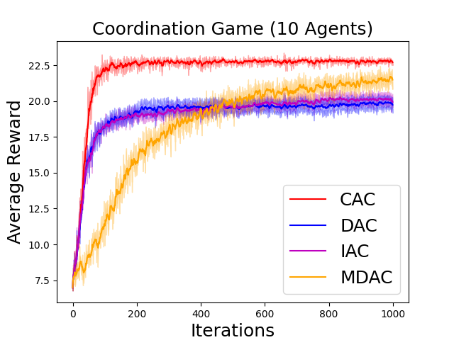
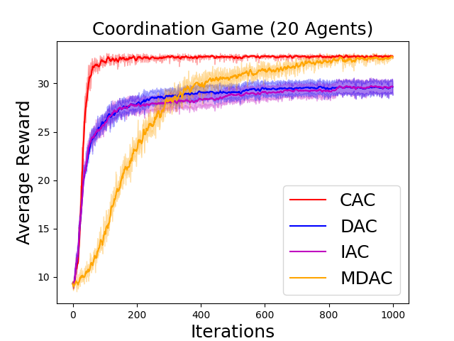
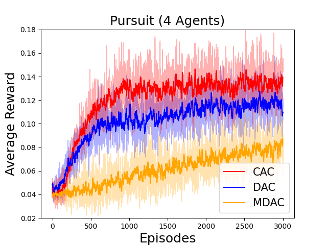
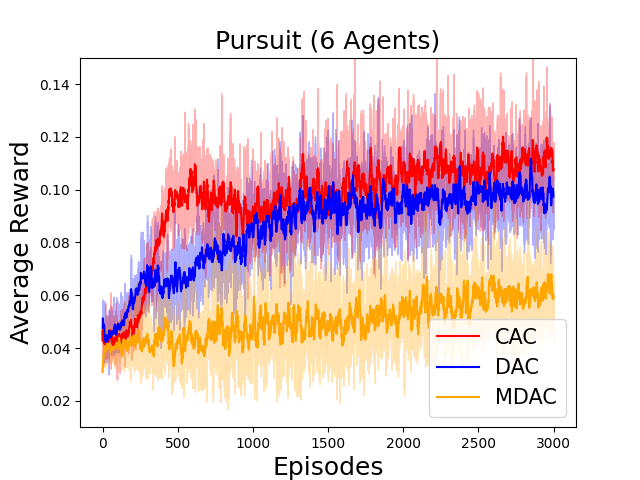
Figure 1: Simulation Results. The averaged reward versus the learning process. The performance is averaged over $10$ Monte Carlo runs.

Pursuit-Evasion Game: there are two groups of nodes, pursuers (agents) and evaders. The pursuers aim to obtain reward through catching evaders. In a two-dimensional environment, an evader is considered caught if two pursuers simultaneously arrive at the evader’s location. In order to catch an evader, each pursuer should learn to cooperate with other pursuers to catch the evaders. From this perspective, the pursuers share some similarities with each other since they need to follow similar strategies to achieve their local tasks: simultaneously catching a same evader with other pursuers. In Figure 1 (two right figures), we compare the numerical performance of the proposed CAC algorithm and two benchmarks: decentralized Actor-Critic (DAC) in [9]; mini-batch decentralized Actor-Critic (MDAC) in [21]. Each agent maintains two convolutional neural networks (CNNs), one for the actor and one for the critic. Please see Figure 2 in Appendix for the structure diagrams of actor network and critic network being used. In the CAC, two convolutional layers of actor network will be regarded as shared policy parameters, and the output layer is personalized (thus not shared).

The two sets of numerical results suggest that, when local tasks share a certain degree of similarity / homogeneity, CAC algorithm with (partial) parameter sharing could achieve more stable convergence.

6 Conclusion

This paper develops a novel collaboration mechanism for designing robust MARL systems. Further, it develops and analyzes a novel multi-agent AC method, where agents are allowed to (partially) share their policy parameters with the neighbors to learn from different agents. To our knowledge, this is the first non-asymptotic convergence result for two-timescale multi-agent AC methods.

Appendix A Experiment Details

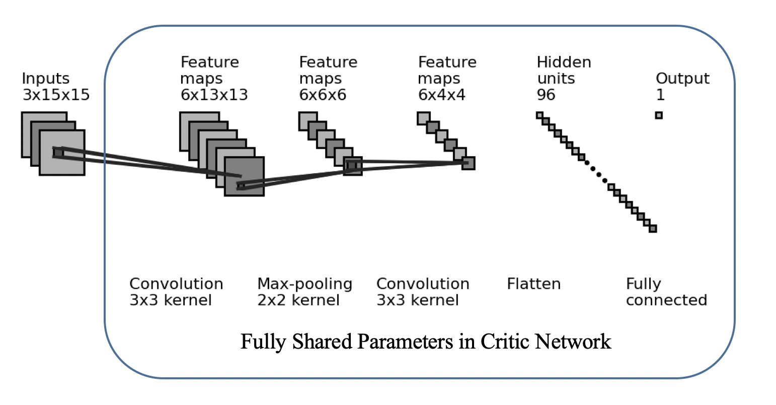
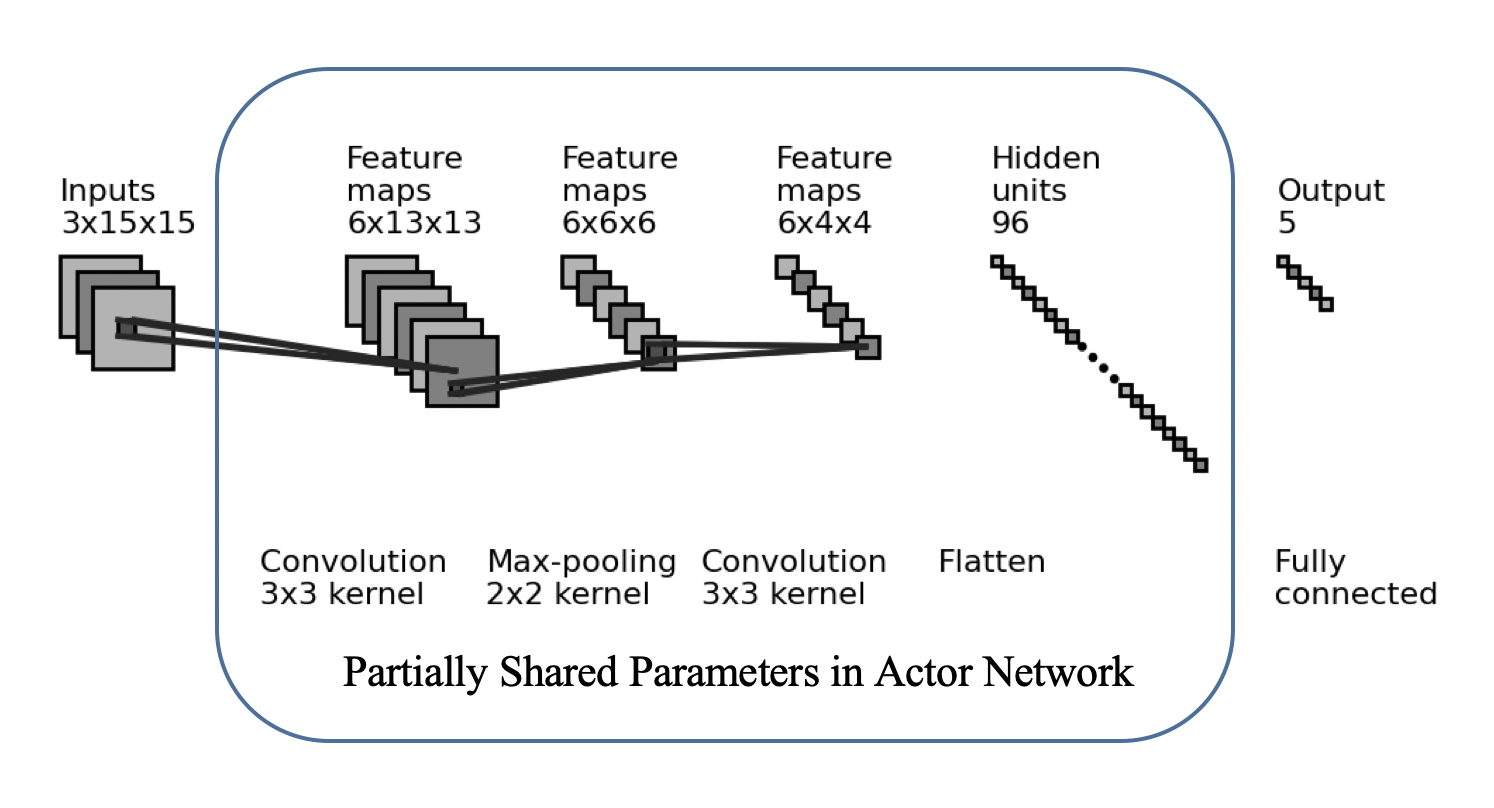
Figure 2: Neural Network Architecture Diagrams for the CAC Algorithm. The architecture diagrams for actor network and critic network of algorithm CAC in the pursuit-evasion Game. (Left) The diagram of critic network. (Right) The diagram of actor network.

In this section, we will present the experiment details on the pursuit-evasion game.

A.1 pursuit-evasion Game

The ‘capture’ reward for each agent is set to be $5$ when a pursuer successfully catches an evader. Moreover, the pursuer will receive a small reward signal which is set to be $0.1$ when the pursuer encounters an evader at its current location. The environment is set to be a $15\times 15$ grid and this 2D grid contains obstacles where the agents cannot pass through. Hence, the global state of the pursuit-evasion game consists of three images (binary matrices) of the size of $15\times 15$. Hence, the dimension of the global state is $3\times 15\times 15$. These three images (binary matrices) respectively present the location of the pursuers, evaders and obstacles in the two-dimensional grid. Only given the 3-channel images as the global state, it is difficult for each pursuer (agent) to distinguish itself with other pursuers since the 3-channel images (global state) does not directly show the ID for each pursuer in the pursuit-evasion Game. To tackle this challenging, we center each agent’s observation at its own location. With a large observation radius, each agent could observe the global information in the environment.

Considering the observation of each agent is a 3-channel image, each agent respectively maintains two convolutional neural networks (CNNs) with two convolutional layers, one max-pooling layer and one fully connected layer for the actor and the critic. Please see Figure 2 for the structure diagrams of actor network and critic network in algorithm CAC. The communication graph $\mathcal{G}_{t}$ between the agents is a complete graph every $20$ iterations, and is not connected for the rest of time. Hence, for CAC algorithm, the global averaging step will be performed on the entire critic networks and the two CNN layers of actor networks every $20$ iterations. The RuLU activation function is utilized in each hidden layer of actor network and critic network. The output of critic network approximates the value function $V_{\pi_{\bm{\theta}}}(s)$ for all $s\in\mathcal{S}$ and the dimension of the output layer is $1$. Furthermore, the output dimension of actor network is $5$ which corresponds to the number of possible actions. In each CNN, the raw images (3-channel location matrices), whose dimension is $3\times 15\times 15$, are processed by two convolutional layers and one max-pooling layer first and then pass through a fully connected layer as the output layer. We utilize the RMSprop optimizer [41] to train neural networks, which is a common choice in training neural networks for reinforcement learning problems [42]. For each algorithm, we set the actor stepsize and critic stepsize as $1\times 10^{-4}$ and $1\times 10^{-3}$. For algorithm MDAC to achieve quick convergence, we tune its batch size and set small batch $B=5$ in its inner loop. The discount factor $\gamma$ is set to be $0.95$ in this simulation.

Appendix B Discussion: Application Scenarios and Potential Benefits

Here, we discuss how the proposed CAC algorithm can be used in two popular multi-agent settings:

$\bullet$ Fully personalized multi-agent RL. The CAC algorithm can be applied to the special setting where the agents do not share their policy parameters with neighbors, and no cooperation is considered in generating the local policies. This setting has been proposed and studied in a number of existing works, such as [9, 43].

$\bullet$ Federated RL. The proposed algorithm can be applied to a general federated (reinforcement) learning setting, where the agents jointly optimize a common objective. To see the connection, let us first describe a standard federated learning (FL) setting [44, 45]: a central controller coordinates a few agents, where the agents continuously optimize their local parameters and perform occasional averaging steps over the parameters. It can be shown that this protocol corresponds to a dynamic setting where $\mathcal{G}_{t}$ is a complete graph every fixed number of iterations, while it is not connected at all for the rest of times (which is a special case of our setting, see Assumption 1). When the network is connected, each agent could gather other agents’ models and perform the averaging; when the network is not connected, then each agent just performs local updates. We generalize the above FL setting to MARL in CAC algorithm.

Although our partially personalized policy structure may be relatively more difficult to analyze, it has a number of potential advantages, as we list below:

$\bullet$ A Generic Model. We use the partial policy sharing as a generic setting, to cover the full spectrum of strategies ranging from no sharing case ($\theta^{s}_{i}=0,\;\forall\leavevmode\nobreak\ i$) to the full sharing case (($\theta^{p}_{i}=0,\;\forall\leavevmode\nobreak\ i$)). This generic model ensures that our subsequent algorithms and analysis can be directly used for all cases.

$\bullet$ Better Models for Homogeneous Agents. When the agents’ local tasks have a high level of similarity (a.k.a. the homogeneous setting), partially sharing models’ parameters could achieve better feature representation and guarantee that the agents’ policies are closely related to each other. Additionally, the shared parameters could leverage more data (i.e., data drawn from all agents) compared with the personalized parameters, so the variance in the training process can be significantly reduced, potentially resulting in better training performance. Such an intuition has been verified empirically in reinforcement learning systems [25, 27, 26], where sharing policies among different learners results in more stable convergence.

$\bullet$ Approximate Common Knowledge. A critical assumption often made in the analysis of multiagent systems is common knowledge [46]. Intuitively, this implies agents have a shared awareness of the underlying interaction. A key difficulty in MARL is that agents are simultaneously learning features of the underlying environment, thus common knowledge is not guaranteed. Thus notions of approximate common knowledge have been proposed for MARL [47]. By relying on (partial) policy sharing mechanism, we hope to have some degree of approximate common knowledge and this is what facilitates coordination.

Appendix C Technical Assumptions

Assumption 5.

Define the score function $\psi_{\bm{\theta}}(s,\bm{a}):=\nabla_{\bm{\theta}}\log\pi_{\bm{\theta}}(\bm{a}\mid s)$. For any policy parameters $\bm{\theta}$ and $\bm{\theta}^{\prime}$, and any state-action $(s,\bm{a})$, the following holds:

$$\|\psi_{\bm{\theta}}(s,\bm{a})-\psi_{\bm{\theta}^{\prime}}(s,\bm{a})\| \leq L_{\psi}\cdot\|\bm{\theta}-\bm{\theta}^{\prime}\|,\quad\|\psi_{\bm{\theta}}(s,\bm{a})\|\leq C_{\psi}\quad$$ (14a)

$$|\pi_{\bm{\theta}}(\bm{a}\mid s)-\pi_{\bm{\theta}^{\prime}}(\bm{a}\mid s)| \leq L_{\pi}\cdot\|\bm{\theta}-\bm{\theta}^{\prime}\|$$ (14b)

where $L_{\pi},L_{\psi},C_{\psi}$ are some constants.

Assumption 5 has been often used in analyzing policy gradient-type algorithms, for example see [48, 49]. Many policy parameterization methods such as tabular softmax policy [49], Gaussian policy [50] and Boltzmann policy [51] satisfy this assumption.

Assumption 6.

For any policy parameters $\bm{\theta}$, the markov chain under policy $\pi_{\bm{\theta}}$ and transition kernel $\mathcal{P}(\cdot|s,\bm{a})$ is irreducible and aperiodic. Then there exist constants $\kappa>0$ and $\tau\in(0,1)$ such that

$$\sup_{s\in\mathcal{S}}\leavevmode\nobreak\ d_{TV}\big{(}\mathcal{P}^{\pi_{\bm{\theta}}}(s_{t}\in\cdot|s_{0}=s),\mu_{\bm{\theta}}(\cdot)\big{)}\leq\kappa\cdot\tau^{t},\quad\forall t$$ (15)

where $d_{TV}(\cdot)$ is the total variation (TV) norm; $\mu_{\theta}$ is the stationary state distribution under $\pi_{\bm{\theta}}$.

Assumption 6 assumes the Markov chain mixes at a geometric rate; see also [35, 52].

Appendix D Auxiliary Lemmas

Lemma 1.

([18, Lemma 1]) Let $\mathcal{X}$ be a nonempty closed convex set in $\mathbb{R}^{K}$, then the following holds:

$$\left(\Pi_{\mathcal{X}}[x]-x\right)^{T}(x-y)\leq-\|\Pi_{\mathcal{X}}[x]-x\|^{2},\;\forall\leavevmode\nobreak\ x\in\mathbb{R}^{K},\;y\in\mathcal{X}$$ (16a)

$$\|\Pi_{\mathcal{X}}[x]-y\|^{2}\leq\|x-y\|^{2}-\|\Pi_{\mathcal{X}}[x]-x\|^{2},\;\forall\leavevmode\nobreak\ x\in\mathbb{R}^{K},\;y\in\mathcal{X}$$ (16b)

where $\Pi_{\cal X}[\cdot]$ denotes the projection operator on to the convex set $\mathcal{X}$.

Lemma 2.

([48, Lemma 3.2]). Suppose Assumption 5 holds. Then the following holds:

$$\|\nabla J(\bm{\theta})-\nabla J(\bm{\theta}^{\prime})\|\leq L_{J}\cdot\|\bm{\theta}-\bm{\theta}^{\prime}\|,\quad\forall\leavevmode\nobreak\ \bm{\theta},\bm{\theta}^{\prime}\in\mathbb{R}^{N\times D}$$ (17)

where $J(\cdot)$ is the objective function defined in (3); $L_{J}:=\frac{R_{\max}\cdot L_{\psi}}{(1-\gamma)^{2}}+\frac{(1+\gamma)\cdot R_{\max}\cdot C_{\psi}^{2}}{(1-\gamma)^{3}}$ with $L_{\psi}$ and $C_{\psi}$ defined in Assumption 5.

Lemma 3.

([38, Lemma 4]). Suppose Assumption 5 holds. The following holds:

$$\|\nabla J(\bm{\theta})\|\leq L_{v},\quad|J(\bm{\theta}_{1})-J(\bm{\theta}_{2})|\leq L_{v}\cdot\|\bm{\theta}_{1}-\bm{\theta}_{2}\|,\;\forall\leavevmode\nobreak\ \bm{\theta},\bm{\theta}^{\prime}\in\mathbb{R}^{N\times D},\;s\in\mathcal{S},$$ (18)

where the constant $L_{v}:=\frac{R_{\max}}{1-\gamma}\cdot C_{\psi}$, with $C_{\psi}$ defined in Assumption 5.

Lemma 4.

([38, Lemma 1]) Suppose Assumption 6 holds. The following holds:

$$d_{TV}(\mu_{\bm{\theta}},d_{\bm{\theta}})\leq 2\left(\log_{\tau}\kappa^{-1}+\frac{1}{1-\tau}\right)(1-\gamma),\quad\forall\leavevmode\nobreak\ \bm{\theta}\in\mathbb{R}^{N\times D}$$ (19)

where $\mu_{\bm{\theta}}(\cdot)$ is the stationary distribution of each state $s$ under policy parameters $\bm{\theta}$ and $d_{\bm{\theta}}(\cdot)$ is the discounted visitation meausre $d_{\bm{\theta}}(s):=(1-\gamma)\sum_{t=0}^{\infty}\gamma^{t}\cdot\mathcal{P}^{\pi_{\bm{\theta}}}(s_{t}=s\mid s_{0}\sim\eta)$.

With the technical assumptions in C, we could bound consensus errors over the iterations. Towards this end, let us provide some basic properties for the weight matrices. Based on Assumptions 1 - 2 which ensure the long-term connectivity and impose the underlying topology of the networked system, we can obtain the following condition [34, Lemma 9]:

$$\|W_{t}\cdots W_{t+B-1}\cdot Q\cdot\bm{\omega}\|\leq\eta\cdot\|Q\cdot\bm{\omega}\|,$$ (20)

when $\bm{\omega}:=[\omega_{1}^{T};\omega_{2}^{T};\cdots;\omega_{N}^{T}]\in\mathbb{R}^{N\times K}$; and we define $Q:=I-\frac{1}{N}\bm{1}\cdot\bm{1}^{T}\in\mathbb{R}^{N\times N}.$ Further, the constant $\eta$ in (20) is given by $\eta:=\sqrt{1-\frac{c}{2N^{2}}}\in(0,1),$ where constant $c$ is defined in Assumption 2.

Based on the above property, we have the following bounds on various consensus errors. Please see Appendix F for the proof.

Lemma 5.

Based on Assumptions 1 - 4, there exist constants $L_{B}>0$ and $\ell_{p}>0$ such that the consensus errors $\|Q\cdot\bm{\omega}_{t}\|+\|Q\cdot\bm{\lambda}_{t}\|$ and $\|Q\cdot\bm{\theta}_{t}^{s}\|$ satisfy

$$\|Q\cdot\bm{\omega}_{t}\|+\|Q\cdot\bm{\lambda}_{t}\|\leq\rho^{t}\cdot\frac{\|\bm{\omega}_{0}\|+\|\bm{\lambda}_{0}\|}{\eta}+\frac{2N\cdot L_{b}\cdot(\beta+\zeta)}{\eta\cdot(1-\rho)}\cdot\frac{1}{T^{\sigma_{2}}}$$ (21a)

$$\|Q\cdot\bm{\theta}_{t}^{s}\|\leq\rho^{t}\cdot\frac{\|\bm{\theta}_{0}^{s}\|}{\eta}+\frac{\ell_{p}\cdot\alpha}{\eta\cdot(1-\rho)}\cdot\frac{1}{T^{\sigma_{1}}}$$ (21b)

$$\frac{1}{T}\sum_{t=0}^{T-1}\bigg{(}\|Q\cdot\bm{\omega}_{t}\|+\|Q\cdot\bm{\lambda}_{t}\|\bigg{)}=\mathcal{O}\bigg{(}T^{-\sigma_{2}}\bigg{)},$$ (21c)

$$\frac{1}{T}\sum_{t=0}^{T-1}\bigg{(}\|Q\cdot\bm{\lambda}_{t}\|^{2}+\|Q\cdot\bm{\omega}_{t}\|^{2}\bigg{)}=\mathcal{O}(T^{-1})+\mathcal{O}(T^{-2\sigma_{2}})$$ (21d)

$$\frac{1}{T}\sum_{t=0}^{T-1}\|Q\cdot\bm{\theta}_{t}^{s}\|=\mathcal{O}\bigg{(}T^{-\sigma_{1}}\bigg{)},\leavevmode\nobreak\ \frac{1}{T}\sum_{t=0}^{T-1}\|Q\cdot\bm{\theta}_{t}^{s}\|^{2}=\mathcal{O}(T^{-1})+\mathcal{O}(T^{-2\sigma_{1}})$$ (21e)

where $\alpha_{t}:=\frac{\alpha}{T^{\sigma_{1}}}$, $\beta_{t}:=\frac{\beta}{T^{\sigma_{2}}}$ and $\zeta_{t}:=\frac{\zeta}{T^{\sigma_{2}}}$ are three stepsizes; $\rho:=\eta^{\frac{1}{\mathcal{B}}}$.

Given the fixed policy parameter $\bm{\theta}$, solving the lower level problem of (8) is equivalent to solving the centralized policy evaluation problems, expressed in (6) and (7). Through the first-order optimality condition, it is easy to show that $w^{*}(\bm{\theta})$ satisfies the following condition:

$$A(\bm{\theta})\cdot\omega^{*}(\bm{\theta})=\frac{1}{N}\sum_{i=1}^{N}b_{i}(\bm{\theta})$$ (22)

where we have defined:

$$A(\bm{\theta}):= \leavevmode\nobreak\ \mathbb{E}_{s\sim\mu_{\bm{\theta}}(\cdot),s^{\prime}\sim\mathcal{P}^{\pi_{\bm{\theta}}}(\cdot|s)}\left[\phi(s)\big{(}\phi(s)-\gamma\cdot\phi(s^{\prime})\big{)}^{T}\right],\;\forall\leavevmode\nobreak\ i\in\mathcal{N},$$ (23a)

$$b_{i}(\bm{\theta}):= \leavevmode\nobreak\ \mathbb{E}_{s\sim\mu_{\bm{\theta}}(\cdot),\bm{a}\sim\pi_{\bm{\theta}}(\cdot|s)}\left[r_{i}(s,a)\cdot\phi(s)\right],\;\forall\leavevmode\nobreak\ i\in\mathcal{N}.$$ (23b)

Under the full-rankness and bounded assumption of the feature matrices given in Assumption 4, we can apply [33, Theorem 2], and show that $A(\bm{\theta})$ is a positive definite matrix for any fixed $\bm{\theta}$. Let us define

$$0<\tilde{c}_{\text{min}}\leq c_{\min}\big{(}A(\bm{\theta})\big{)},\quad 0<c_{\max}\big{(}A(\bm{\theta})\big{)}\leq\tilde{c}_{\text{max}},\leavevmode\nobreak\ \forall\leavevmode\nobreak\ \bm{\theta}\in\mathbb{R}^{N\times D},$$ (24)

where $c_{\min}\big{(}A(\bm{\theta})\big{)}$ and $c_{\max}\big{(}A(\bm{\theta})\big{)}$ are the minimum and maximum eigenvalue of $A(\bm{\theta})$; $\tilde{c}_{\text{min}}$ and $\tilde{c}_{\text{max}}$ are the lower bound and upper bound on the eigenvalues of $A(\bm{\theta})$. Then we have the following Lipschitz property of the optimal critic parameters.

Lemma 6.

([38, Proposition 2 ]) Suppose Assumptions 4,5,6 hold. Let $w^{*}(\bm{\theta})$ denote the optimal solution in (7) to approximate value function approximation. Then the following Lipschitz condition holds:

$$\|\omega^{*}(\bm{\theta}_{1})-\omega^{*}(\bm{\theta}_{2})\|\leq L_{\omega}\cdot\|\bm{\theta}_{1}-\bm{\theta}_{2}\|,\quad\forall\leavevmode\nobreak\ \bm{\theta}_{1},\bm{\theta}_{2}\in\mathbb{R}^{N\times D},$$ (25)

where $L_{\omega}:=2\cdot R_{\max}\cdot|\mathcal{A}|\cdot L_{\pi}\cdot\bigg{(}\tilde{c}_{\min}^{-1}+\tilde{c}_{\min}^{-2}\cdot(1+\gamma)\bigg{)}\bigg{(}1+\log_{\tau}\kappa^{-1}+(1-\tau)^{-1}\bigg{)}$.

Appendix E Discussion: Convergence Results

In this section, we discuss an extension of Theorem 1.

As a special case, when the agents do not share any policy parameters, that is, when $\bm{\theta}=\bm{\theta}^{p}$, the resulting algorithm reduces to the standard Decentralized AC algorithm and we name it as Coordinated Actor-Critic with no policy sharing (CAC-NPS), whose asymptotic convergence property has been analyzed in [9]. The non-asymptotic convergence rate for this algorithm can be readily obtained from (a slightly modified versions of) Proposition 1 – 2. The following result states the convergence rate for CAC-NPS, and we refer the readers to Appendix H for detailed proof steps.

Corollary 2.

(Convergence of CAC-NPS Algorithm) Suppose Assumptions 1 - 6 hold. Consider applying Algorithm 1 to a problem with fully-personalized policy parameters, that is, $\bm{\theta}:=\cup_{i=1}^{N}\{\theta^{p}_{i}\}$. Setting $\sigma_{1}=\frac{3}{5}$ and $\sigma_{2}=\frac{2}{5}$, then the following holds:

$$\frac{1}{T}\sum_{t=0}^{T-1}\sum_{i=1}^{N}\bigg{(}\mathbb{E}\bigg{[}\|\omega_{i,t}-\omega^{*}(\bm{\theta}_{t})\|^{2}\bigg{]}+\mathbb{E}\bigg{[}\|\lambda_{i,t}-\lambda^{*}(\bm{\theta}_{t})\|^{2}\bigg{]}\bigg{)}=\mathcal{O}(T^{-\frac{2}{5}})$$ (26)

$$\frac{1}{T}\sum_{t=0}^{T-1}\sum_{i=1}^{N}\mathbb{E}\bigg{[}\|\nabla_{\theta_{i}}J(\bm{\theta}_{t})\|^{2}\bigg{]}=\mathcal{O}(T^{-\frac{2}{5}})+\mathcal{O}(\epsilon_{app}+\epsilon_{sp}).$$ (27)

The critic approximation error $\epsilon_{app}$ and the sampling error $\epsilon_{sp}$ are defined as follows [36, 38]:

$$\epsilon_{\text{app}} :=\max_{\bm{\theta}}\sqrt{\mathop{\mathbb{E}}\limits_{\begin{subarray}{c}s\sim\mu_{\bm{\theta}}(\cdot)\end{subarray}}\left[\bigg{(}V_{\pi_{\bm{\theta}}}(s)-\phi(s)^{T}\omega^{*}(\bm{\theta})\bigg{)}^{2}\right]}+\sqrt{\mathop{\mathbb{E}}\limits_{\begin{subarray}{c}s\sim\mu_{\bm{\theta}}(\cdot)\\ a\sim\pi_{\bm{\theta}}(\cdot)\end{subarray}}\left[\bigg{(}\bar{r}(s,\bm{a})-\varphi(s,\bm{a})^{T}\lambda^{*}(\bm{\theta})\bigg{)}^{2}\right]}$$ (28)

$$\epsilon_{\text{sp}} :=4\cdot R_{\max}\cdot C_{\psi}\cdot L_{v}\cdot\left(\log_{\tau}\kappa^{-1}+\frac{1}{1-\tau}\right)$$ (29)

where $\mu_{\bm{\theta}}(\cdot)$ is the stationary distribution of state under policy $\pi_{\bm{\theta}}$ and the transition kernel $\mathcal{P}(\cdot)$.

Appendix F Proof of Lemma 5

The proof of Lemma 5 is divided into two steps. In step 1, we first analyze the consensus error $\|Q\cdot\bm{\omega}_{t}\|$ and then extend the analysis results to $\|Q\cdot\bm{\lambda}_{t}\|$. In step 2, we further analyze the consensus error $\|Q\cdot\bm{\theta}_{t}^{s}\|$ in the shared part of policy parameters.

Step 1..

Since the mixing matrix $W_{t}$ is doubly stochastic so $W_{t}\cdot\bm{1}=\bm{1}$, where $\bm{1}$ is a column vector of all ones. We obtain that

$$W_{t}\cdot\bm{\omega}_{t}-\bm{1}\cdot\bar{\omega}_{t}^{T}=W_{t}\cdot\left(\bm{\omega}_{t}-\bm{1}\cdot\bar{\omega}_{t}^{T}\right).$$

By the definition of locally estimated TD error in (13), it follows that

$$\delta_{i,t} :=r_{i,t}+\gamma\cdot\widehat{V}(s_{t+1};\omega_{i,t})-\widehat{V}(s_{t};\omega_{i,t})$$

$$=r_{i,t}+\gamma\cdot\phi(s_{t+1})^{T}\omega_{i,t}-\phi(s_{t})^{T}\omega_{i,t}$$ (30)

where $\phi(\cdot)\in\mathbb{R}^{K}$ is the feature mapping for any state $s\in\mathcal{S}$. To perform the critic step according to equation (13), it holds that

$$\omega_{i,t}=\Pi_{R_{\omega}}\bigg{(}\sum_{j\in\mathcal{N}_{i}(t)}W_{t-1}^{ij}\omega_{i,t-1}+\beta_{t}\cdot\delta_{i,t-1}\cdot\nabla_{\omega_{i}}\widehat{V}(s_{t-1};\omega_{i,t-1})\bigg{)},$$

$$=\Pi_{R_{\omega}}\bigg{(}\sum_{j\in\mathcal{N}_{i}(t)}W_{t-1}^{ij}\omega_{i,t-1}+\beta_{t}\cdot\delta_{i,t-1}\cdot\phi(s_{t-1})\bigg{)},\quad\forall i\in\mathcal{N}$$ (31)

where $\nabla_{\omega_{i}}\widehat{V}(s_{t-1};\omega_{i,t-1}):=\phi(s_{t-1})$ due to linear parameterization. Recall that $A(\bm{\theta}_{t})$, $b_{i}(\bm{\theta}_{t})$ are defined in (23), it holds that

$$b_{i}(\bm{\theta}_{t})-A(\bm{\theta}_{t})\cdot\omega_{i,t} :=\mathbb{E}_{s\sim\mu_{\bm{\theta}_{t}}(\cdot),\bm{a}\sim\pi_{\bm{\theta}_{t}}(\cdot|s),s^{\prime}\sim\mathcal{P}(\cdot|s,\bm{a})}\bigg{[}\big{(}r_{i}(s,a)+\gamma\cdot\phi(s)^{T}\omega_{i,t}-\phi(s^{\prime})^{T}\omega_{i,t}\big{)}\cdot\phi(s)\bigg{]}$$

$$=\mathbb{E}_{s_{t}\sim\mu_{\bm{\theta}_{t}}(\cdot),\bm{a}_{t}\sim\pi_{\bm{\theta}_{t}}(\cdot|s_{t}),s_{t+1}\sim\mathcal{P}(\cdot|s_{t},\bm{a}_{t})}\bigg{[}\delta_{i,t}\cdot\phi(s_{t})\bigg{]}.$$ (32)

Hence, in (31) the estimated stochastic gradient at each iteration $t$ is expressed as

$$\delta_{i,t}\cdot\phi(s_{t}) =\underbrace{\bigg{(}\delta_{i,t}\cdot\phi(s_{t})-[b_{i}(\bm{\theta}_{t})-A(\bm{\theta}_{t})\cdot\omega_{i,t}]\bigg{)}}_{:=m_{i,t}}+\underbrace{\bigg{(}b_{i}(\bm{\theta}_{t})-A(\bm{\theta}_{t})\cdot\omega_{i,t}\bigg{)}}_{:=h_{i,t}}$$ (33)

where $h_{i,t}$ is the expectation of the estimated stochastic gradient $\delta_{i,t}\cdot\phi(s_{t})$; $m_{i,t}$ denotes the deviation between $\delta_{i,t}\cdot\phi(s_{t})$ and its expectation $h_{i,t}$.

Recall that the subroutine to update critic parameters $\bm{\omega}_{t}$ in (13) is given below:

$$\widetilde{\bm{\omega}}_{t-1}=W_{t-1}\cdot\bm{\omega}_{t-1},\quad\omega_{i,t}=\Pi_{R_{\omega}}\bigg{(}\widetilde{\omega}_{i,t-1}+\beta_{t-1}\cdot\delta_{i,t-1}\cdot\nabla_{\omega_{i}}\widehat{V}(s_{t-1};\omega_{i,t-1})\bigg{)},\leavevmode\nobreak\ \forall i\in\mathcal{N}.$$ (34)

It can be decomposed using the following steps:

$$\widetilde{\omega}_{i,t-1} =\sum_{j\in\mathcal{N}_{i}(t-1)}W_{t-1}^{ij}\cdot\omega_{i,t-1}$$ (35a)

$$y_{i,t-1} \stackrel{{\scriptstyle\eqref{eq:delta:phi}}}{{=}}\widetilde{\omega}_{i,t-1}+\beta_{t-1}\cdot(h_{i,t-1}+m_{i,t-1})$$ (35b)

$$e_{i,t-1} =y_{i,t-1}-\Pi_{R_{\omega}}(y_{i,t-1})$$ (35c)

$$\omega_{i,t} =\Pi_{R_{\omega}}(y_{i,t-1})=y_{i,t-1}-e_{i,t-1}.$$ (35d)

Express the above updates in matrix form, it holds that

$$\widetilde{\bm{\omega}}_{t-1} =W_{t-1}\cdot\bm{\omega}_{t-1}$$ (36a)

$$\bm{y}_{t-1} =\widetilde{\bm{\omega}}_{t-1}+\beta_{t-1}\cdot(\bm{h}_{t-1}+\bm{m}_{t-1})$$ (36b)

$$\bm{e}_{t-1} =\bm{y}_{t-1}-\Pi_{R_{\omega}}(\bm{y}_{t-1})$$ (36c)

$$\bm{\omega}_{t} =\bm{y}_{t-1}-\bm{e}_{t-1}$$ (36d)

where $\bm{y}_{t},\bm{h}_{t},\bm{m}_{t},\bm{e}_{t}$ correspond to the collections of local vectors $\{y_{i,t}\},\{h_{i,t}\},\{m_{i,t}\},\{e_{i,t}\}$. Recall the definitions $\bm{\omega}_{t}=[\omega_{1,t}^{T};\omega_{2,t}^{T};\cdots;\omega_{N,t}^{T}]\in\mathbb{R}^{N\times K}$ and $\bar{\omega}_{t}^{T}:=\frac{1}{N}\bm{1}^{T}\bm{\omega}_{t}$, it follows

$$\bar{\omega}_{t}^{T} =\frac{1}{N}\bm{1}^{T}\bm{\omega}_{t}$$

$$\overset{(i)}{=}\frac{1}{N}\bm{1}^{T}\big{(}W_{t-1}\cdot\bm{\omega}_{t-1}+\beta_{t-1}\cdot(\bm{h}_{t-1}+\bm{m}_{t-1})-\bm{e}_{t-1}\big{)}$$

$$\overset{(ii)}{=}\bar{\omega}_{t-1}^{T}+\beta_{t-1}\cdot(\bar{h}_{t-1}^{T}+\bar{m}_{t-1}^{T})-\bar{e}_{t-1}^{T}$$ (37)

where $\bar{h}_{t-1}$, $\bar{m}_{t-1}$ and $\bar{e}_{t-1}$ are the averaged vectors of $\mathbf{h}_{t-1}$, $\mathbf{m}_{t-1}$ and $\mathbf{e}_{t-1}$ (as defined similarly as $\bar{\omega}_{t-1}$); $(i)$ is from the subroutine (36); $(ii)$ is from $\bm{1}^{T}W_{t-1}=\bm{1}^{T}$ due to double stochasticity in weight matrix $W_{t-1}$. Recall that we have defined $Q=I-\frac{1}{N}\bm{1}\cdot\bm{1}^{T}$, then it is clear that $Q\cdot\bm{\omega}$ indicates the consensus error. We can express such an error as follows:

$$Q\cdot\bm{\omega}_{t} =\bm{\omega}_{t}-\bm{1}\bar{\omega}_{t}^{T}$$

$$=W_{t-1}\cdot\bm{\omega}_{t-1}+\beta_{t-1}\cdot\left(\bm{h}_{t-1}+\bm{m}_{t-1}\right)-\bm{e}_{t-1}-[\bm{1}\bar{\omega}_{t-1}^{T}+\beta_{t-1}\cdot\bm{1}[\bar{h}_{t-1}+\bar{m}_{t-1}]^{T}-\bm{1}\bar{e}_{t-1}^{T}]$$

$$=W_{t-1}\cdot\left(\bm{\omega}_{t-1}-\bm{1}\bar{\omega}_{t-1}^{T}\right)+\beta_{t-1}\cdot\left(\bm{h}_{t-1}-\bm{1}\bar{h}_{t-1}^{T}\right)+\beta_{t-1}\cdot\left(\bm{m}_{t-1}-\bm{1}\bar{m}_{t-1}^{T}\right)-\left(\bm{e}_{t-1}-\bm{1}\bar{e}_{t-1}^{T}\right)$$

$$=W_{t-1}\cdot Q\cdot\bm{\omega}_{t-1}+\beta_{t-1}\cdot Q\cdot(\bm{h}_{t-1}+\bm{m}_{t-1})-Q\cdot\bm{e}_{t-1}$$ (38)

$$=\left(\Pi_{k=0}^{t-1}W_{k}\right)\cdot Q\cdot\bm{\omega}_{0}-\sum_{k=0}^{t-1}(\Pi_{\ell=k+1}^{t-1}W_{\ell})\cdot Q\cdot\bm{e}_{k}+\sum_{k=0}^{t-1}\beta_{k}\cdot(\Pi_{\ell=k+1}^{t-1}W_{\ell})\cdot Q\cdot\left(\bm{h}_{k}+\bm{m}_{k}\right).$$ (39)

Then we can bound the norm of the consensus error using the following:

$$\|Q\cdot\bm{\omega}_{t}\| \overset{(i)}{\leq}\|(\Pi_{k=0}^{t-1}W_{k})\cdot Q\cdot\bm{\omega}_{0}\|+\sum_{k=0}^{t-1}\|(\Pi_{\ell=k+1}^{t-1}W_{\ell})\cdot Q\cdot\bm{e}_{k-1}\|$$

$$\quad+\sum_{k=0}^{t-1}\beta_{k}\|(\Pi_{\ell=k+1}^{t-1}W_{\ell})\cdot Q\cdot\left(\bm{h}_{k}+\bm{m}_{k}\right)\|$$

$$\overset{(ii)}{\leq}\eta^{\lfloor t/B\rfloor}\cdot\|\bm{\omega}_{0}\|+\sum_{k=0}^{t-1}\eta^{\lfloor(t-k-1)/B\rfloor}\cdot\|\bm{e}_{k}\|+\sum_{k=0}^{t-1}\eta^{\lfloor(t-k-1)/B\rfloor}\cdot\beta_{k}\cdot\|\bm{h}_{k}+\bm{m}_{k}\|$$

$$\overset{(iii)}{\leq}\frac{1}{\eta}\cdot\rho^{t}\cdot\|\bm{\omega}_{0}\|+\frac{1}{\eta}\sum_{k=0}^{t-1}\rho^{t-k-1}\cdot\|\bm{e}_{k}\|+\frac{1}{\eta}\sum_{k=0}^{t-1}\rho^{t-k-1}\cdot\beta_{k}\cdot\|\bm{h}_{k}+\bm{m}_{k}\|$$ (40)

where (ii) follows (20); in (iii) we utilize that $\eta^{\lfloor t/B\rfloor}\leq\eta^{t/B-1}=\frac{1}{\eta}\cdot\rho^{t}$ where we define $\rho:=\eta^{\frac{1}{B}}$.

Next we bound $\|\bm{h}_{k}+\bm{m}_{k}\|$ and $\|\bm{e}_{k}\|$. We have

$$\|h_{i,t}\|+\|m_{i,t}\| \overset{\eqref{eq:delta:phi}}{=}\bigg{\|}\delta_{i,t}\cdot\phi(s_{t})-[b_{i}(\bm{\theta}_{t})-A(\bm{\theta}_{t})\cdot\omega_{i,t}]\bigg{\|}+\bigg{\|}b_{i}(\bm{\theta}_{t})-A(\bm{\theta}_{t})\cdot\omega_{i,t}\bigg{\|}$$

$$\leq\|\delta_{i,t}\cdot\phi(s_{t})\|+2\cdot\|b_{i}(\bm{\theta}_{t})-A(\bm{\theta}_{t})\cdot\omega_{i,t}\|$$

$$\overset{\eqref{eq: TD fixed point}}{=}\|\delta_{i,t}\cdot\phi(s_{t})\|+2\cdot\bigg{\|}\mathbb{E}_{s\sim\mu_{\bm{\theta}_{t}}(\cdot),\bm{a}\sim\pi_{\bm{\theta}_{t}}(\cdot|s),s^{\prime}\sim\mathcal{P}(\cdot|s,\bm{a})}\bigg{[}\big{(}r_{i}(s,a)+\gamma\cdot\phi(s)^{T}\omega_{i,t}-\phi(s^{\prime})^{T}\omega_{i,t}\big{)}\cdot\phi(s)\bigg{]}\bigg{\|}$$

$$\overset{(i)}{\leq}\|\delta_{i,t}\cdot\phi(s_{t})\|+2\cdot\mathbb{E}_{s\sim\mu_{\bm{\theta}_{t}}(\cdot),\bm{a}\sim\pi_{\bm{\theta}_{t}}(\cdot|s),s^{\prime}\sim\mathcal{P}(\cdot|s,\bm{a})}\bigg{[}\bigg{\|}\big{(}r_{i}(s,a)+\gamma\cdot\phi(s)^{T}\omega_{i,t}-\phi(s^{\prime})^{T}\omega_{i,t}\big{)}\cdot\phi(s)\bigg{\|}\bigg{]}$$

$$\overset{(ii)}{\leq}\|\delta_{i,t}\|+2\cdot\mathbb{E}_{s\sim\mu_{\bm{\theta}_{t}}(\cdot),\bm{a}\sim\pi_{\bm{\theta}_{t}}(\cdot|s),s^{\prime}\sim\mathcal{P}(\cdot|s,\bm{a})}\bigg{[}\bigg{\|}\big{(}r_{i}(s,a)+\gamma\cdot\phi(s)^{T}\omega_{i,t}-\phi(s^{\prime})^{T}\omega_{i,t}\big{)}\bigg{\|}\bigg{]}$$

$$\overset{\eqref{eq:delta}}{=}\bigg{\|}r_{i,t}+\gamma\cdot\phi(s_{t+1})^{T}\omega_{i,t}-\phi(s_{t})^{T}\omega_{i,t}\bigg{\|}$$

$$\quad+2\cdot\mathbb{E}_{s\sim\mu_{\bm{\theta}_{t}}(\cdot),\bm{a}\sim\pi_{\bm{\theta}_{t}}(\cdot|s),s^{\prime}\sim\mathcal{P}(\cdot|s,\bm{a})}\bigg{[}\bigg{\|}\big{(}r_{i}(s,a)+\gamma\cdot\phi(s)^{T}\omega_{i,t}-\phi(s^{\prime})^{T}\omega_{i,t}\big{)}\bigg{\|}\bigg{]}$$

$$\overset{(iii)}{\leq}3R_{\max}+3(1+\gamma)\cdot R_{\omega}$$ (41)

where $(i)$ follows Jensen’s inequality; $(ii)$ follows Assumption 4 that $\|\phi(s)\|\leq 1$ for any $s\in\mathcal{S}$; $(iii)$ follows the fact that $|r_{i}(s,a)|\leq R_{\max}$ and the critic parameter $\omega_{i,t}$ is constrained in a fixed region $\|\omega_{i,t}\|\leq R_{\omega}$. For simplicity, in the following part we denote $L_{b}:=3R_{\max}+3(1+\gamma)\cdot R_{\omega}$.

Moreover, it holds that

$$\|e_{i,t}\|\stackrel{{\scriptstyle\eqref{subroutine:critic_update}}}{{=}}\|y_{i,t}-\Pi_{R_{\omega}}(y_{i,t})\|\overset{(i)}{\leq}\|\widetilde{\omega}_{i,t}-y_{i,t}\|=\|\beta_{t}\cdot\left(h_{i,t}+m_{i,t}\right)\|\overset{(ii)}{\leq}\beta_{t}\cdot L_{b},$$ (42)

where $(i)$ follows from (16b) and $(ii)$ follows from (41).

Recall that the stepsizes in critic steps are defined as $\beta_{t}:=\frac{\beta}{T^{\sigma_{2}}},\leavevmode\nobreak\ \forall t$. Plugging (41) and (42) into (40), we get

$$\|Q\cdot\bm{\omega}_{t}\| \leq\frac{1}{\eta}\cdot\rho^{t}\cdot\|\bm{\omega}_{0}\|+\frac{1}{\eta}\sum_{k=0}^{t-1}\rho^{t-k-1}\cdot\beta_{k}\cdot L_{b}\cdot N+\frac{1}{\eta}\sum_{k=0}^{t-1}\rho^{t-k-1}\cdot\beta_{k}\cdot L_{b}\cdot N$$ (43)

$$=\frac{1}{\eta}\cdot\rho^{t}\cdot\|\bm{\omega}_{0}\|+\frac{2N\cdot L_{b}\cdot\beta}{\eta\cdot T^{\sigma_{2}}}\cdot\sum_{k=0}^{t-1}\rho^{t-k-1}$$

$$\overset{(a)}{\leq}\frac{1}{\eta}\cdot\rho^{t}\cdot\|\bm{\omega}_{0}\|+\frac{2N\cdot L_{b}\cdot\beta}{\eta\cdot T^{\sigma_{2}}}\cdot\frac{1}{1-\rho}$$ (44)

where $(a)$ follows the fact that $\sum_{k=0}^{t-1}\rho^{t-k-1}\leq\frac{1}{1-\rho},\leavevmode\nobreak\ \forall t$.

Summing (44) from $t=0$ to $t=T-1$, we obtain

$$\sum_{t=0}^{T-1}\|Q\cdot\bm{\omega}_{t}\| \leq\frac{\|\bm{\omega}_{0}\|}{\eta}\sum_{t=0}^{T-1}\rho^{t}+T\cdot\frac{2N\cdot L_{b}\cdot\beta}{\eta\cdot T^{\sigma_{2}}}\cdot\frac{1}{1-\rho}$$

$$\overset{(i)}{\leq}\frac{\|\bm{\omega}_{0}\|}{\eta\cdot(1-\rho)}+\frac{2N\cdot L_{b}\cdot\beta}{\eta\cdot(1-\rho)}\cdot T^{1-\sigma_{2}},$$ (45)

where $(i)$ is due to the fact that $\sum_{t=0}^{T-1}\rho^{t}\leq\frac{1}{1-\rho}$.

In summary, we obtain the following bound on the averaged consensus violation:

$$\frac{1}{T}\sum_{t=0}^{T-1}\|Q\cdot\bm{\omega}_{t}\|\leq\frac{1}{T}\cdot\frac{\|\bm{\omega}_{0}\|}{\eta\cdot(1-\rho)}++\frac{2N\cdot L_{b}\cdot\beta}{\eta\cdot(1-\rho)}\cdot T^{-\sigma_{2}}.$$ (46)

Extending above analysis steps on deriving a bound for the consensus error $\|Q\cdot\bm{\omega}_{t}\|$ in (45) to $\|Q\cdot\bm{\lambda}_{t}\|$, we can show that the following holds:

$$\|Q\cdot\bm{\lambda}_{t}\|\leq\frac{1}{\eta}\cdot\rho^{t}\cdot\|\bm{\lambda}_{0}\|+\frac{2N\cdot L_{b}\cdot\zeta}{\eta\cdot T^{\sigma_{2}}}\cdot\frac{1}{1-\rho}$$ (47)

where the stepsize $\zeta_{t}$ is defined as $\zeta_{t}:=\frac{\zeta}{T^{\sigma_{2}}}$. Similar as (45), summing up (47) from $t=0$ to $t=T-1$, it holds that:

$$\sum_{t=0}^{T-1}\|Q\cdot\bm{\lambda}_{t}\|\leq\frac{\|\bm{\lambda}_{0}\|}{\eta\cdot(1-\rho)}++\frac{2N\cdot L_{b}\cdot\zeta}{\eta\cdot(1-\rho)}\cdot T^{1-\sigma_{2}}.$$ (48)

In summary, we have

$$\frac{1}{T}\sum_{t=0}^{T-1}\|Q\cdot\bm{\lambda}_{t}\|\leq\frac{1}{T}\cdot\frac{\|\bm{\omega}_{0}\|}{\eta\cdot(1-\rho)}++\frac{2N\cdot L_{b}\cdot\zeta}{\eta\cdot(1-\rho)}\cdot T^{-\sigma_{2}}.$$ (49)

Summing up (46) and (49), we obtain the convergence rate of the consensus errors:

$$\frac{1}{T}\sum_{t=0}^{T-1}\bigg{(}\|Q\cdot\bm{\omega}_{t}\|+\|Q\cdot\bm{\lambda}_{t}\|\bigg{)} =\frac{1}{T}\cdot\frac{\|\bm{\omega}_{0}\|+\|\bm{\lambda}_{0}\|}{\eta\cdot(1-\rho)}+\frac{1}{T^{\sigma_{2}}}\cdot\frac{2N\cdot L_{b}\cdot(\beta+\zeta)}{\eta\cdot(1-\rho)}$$

$$=\mathcal{O}(T^{-\sigma_{2}}).$$ (50)

Taking square on both side of (44) and applying Cauchy-Schwarz inequality, it holds that

$$\|Q\cdot\bm{\omega}_{t}\|^{2} \leq\frac{2}{\eta^{2}}\cdot\rho^{2t}\cdot\|\bm{\omega}_{0}\|^{2}+\frac{2}{T^{2\sigma_{2}}}\cdot\bigg{(}\frac{2N\cdot L_{b}\cdot\beta}{\eta\cdot(1-\rho)}\bigg{)}^{2}$$ (51)

Summing (51) from $t=0$ to $t=T-1$, it holds that

$$\sum_{t=0}^{T-1}\|Q\cdot\bm{\omega}_{t}\|^{2} \leq\frac{2\|\bm{\omega}_{0}\|^{2}}{\eta^{2}\cdot(1-\rho^{2})}+2\cdot\bigg{(}\frac{2N\cdot L_{b}\cdot\beta}{\eta\cdot(1-\rho)}\bigg{)}^{2}\cdot T^{1-2\sigma_{2}}$$ (52)

Extending above analysis steps on deriving a bound for the consensus error $\|Q\cdot\bm{\omega}_{t}\|^{2}$ in (52) to $\|Q\cdot\bm{\lambda}_{t}\|^{2}$, we can show that the following holds:

$$\sum_{t=0}^{T-1}\|Q\cdot\bm{\lambda}_{t}\|^{2} \leq\frac{2\|\bm{\lambda}_{0}\|^{2}}{\eta^{2}\cdot(1-\rho^{2})}+2\cdot\bigg{(}\frac{2N\cdot L_{b}\cdot\zeta}{\eta\cdot(1-\rho)}\bigg{)}^{2}\cdot T^{1-2\sigma_{2}}$$ (53)

Hence, adding (52) and (53), then divide both side by $T$, it holds that

$$\frac{1}{T}\sum_{t=0}^{T-1}\bigg{(}\|Q\cdot\bm{\lambda}_{t}\|^{2}+\|Q\cdot\bm{\omega}_{t}\|^{2}\bigg{)} \leq\frac{2(\|\bm{\lambda}_{0}\|^{2}+\|\bm{\omega}_{0}\|^{2})}{T\cdot\eta^{2}\cdot(1-\rho^{2})}+\frac{8N^{2}\cdot L_{b}^{2}\cdot(\zeta^{2}+\beta^{2})}{\eta^{2}\cdot(1-\rho)^{2}}\cdot T^{-2\sigma_{2}}$$

$$=\mathcal{O}(T^{-1})+\mathcal{O}(T^{-2\sigma_{2}})$$ (54)

This completes the proof for the first part. ∎

Step 2..

In this part, we analyze the consensus errors for the shared policy parameters $\bm{\theta}^{s}$.

Since the mixing matrix $W_{t}$ is doubly stochastic which implies $W_{t}\cdot\bm{1}=\bm{1}$, we obtain that

$$W_{t}\cdot\bm{\theta}_{t}^{s}-\bm{1}\bar{\theta}_{t}^{s^{T}}=W_{t}\cdot\left(\bm{\theta}_{t}^{s}-\bm{1}\bar{\theta}_{t}^{s^{T}}\right)$$

where we have defined $\bar{\theta}_{t}^{s^{T}}:=\frac{1}{N}\bm{1}^{T}\bm{\theta}_{t}^{s}$. Recall that the subroutine to update shared policy parameters in (9) - (10) is given below:

$$\theta_{i,t}^{s} :=\sum_{j\in\mathcal{N}_{i}(t-1)}W_{t-1}^{ij}\theta^{s}_{j,t-1}+\alpha_{t-1}\cdot\widehat{\delta}_{i,t-1}\cdot\nabla_{\theta_{i}^{s}}\log\pi_{i}(a_{i,t-1}|s_{t-1},\theta_{i,t-1}),\leavevmode\nobreak\ \leavevmode\nobreak\ \forall i\in\mathcal{N}$$ (55)

where we have defined

$$\widehat{\delta}_{i,t-1} :=\widehat{r}(s_{t-1},\bm{a}_{t-1};\lambda_{i,t-1})+\gamma\cdot\widehat{V}(s_{t};\omega_{i,t-1})-\widehat{V}(s_{t-1};\omega_{i,t-1})$$

$$=\varphi(s_{t-1},\bm{a}_{t-1})^{T}\lambda_{i,t-1}+\gamma\cdot\phi(s_{t-1})^{T}\omega_{i,t-1}-\phi(s_{t})^{T}\omega_{i,t}.$$ (56)

Then we define $g_{i,t-1}:=\widehat{\delta}_{i,t-1}\cdot\nabla_{\theta_{i}^{s}}\log\pi_{i}(a_{i,t-1}|s_{t-1},\theta_{i,t-1})$ and $\bm{g}:=[g_{1}^{T};g_{2}^{T};\cdots;g_{N}^{T}]$, it holds that

$$\bm{\theta}_{t}^{s}:=W_{t-1}\cdot\bm{\theta}_{t-1}^{s}+\alpha_{t-1}\cdot\bm{g}_{t-1}.$$ (57)

Recall $Q=I-\frac{1}{N}\bm{1}\cdot\bm{1}^{T}$, we analyze the consensus error $Q\cdot\bm{\theta}_{t}^{s}$ as below:

$$Q\cdot\bm{\theta}_{t}^{s}= \bm{\theta}_{t}^{s}-\bm{1}\bar{\theta}_{t}^{s^{T}}$$

$$= \bigg{(}W_{t-1}\cdot\bm{\theta}_{t-1}^{s}+\alpha_{t-1}\cdot\bm{g}_{t-1}\bigg{)}-\bigg{(}\bm{1}\bar{\theta}_{t-1}^{s^{T}}+\alpha_{t-1}\cdot\bm{1}\bar{g}_{t-1}^{T}\bigg{)}$$

$$= W_{t-1}\cdot Q\cdot\bm{\theta}_{t-1}^{s}+\alpha_{t-1}\cdot Q\cdot\bm{g}_{t-1}$$

$$= (\Pi_{k=0}^{t-1}W_{k})\cdot Q\cdot\bm{\theta}_{0}^{s}+\sum_{k=0}^{t-1}\alpha_{k}\cdot(\Pi_{l=k+1}^{t-1}W_{l})\cdot Q\cdot\bm{g}_{k}.$$ (58)

By Assumptions 3 - 4, 5, the estimated stochastic gradient $\bm{g}_{t}=[g_{1,t}^{T},g_{2,t}^{T},\cdots,g_{N,t}^{T}]$ can be bounded as below:

$$\|\bm{g}_{t}\| \overset{(i)}{\leq}\sum_{i=1}^{N}\|g_{i,t}\|$$

$$=\sum_{i=1}^{N}\|\widehat{\delta}_{i,t-1}\cdot\nabla_{\theta_{i}^{s}}\log\pi_{i}(a_{i,t-1}|s_{t-1},\theta_{i,t-1})\|$$

$$\overset{(ii)}{\leq}C_{\psi}\cdot\sum_{i=1}^{N}\bigg{\|}\varphi(s_{t-1},\bm{a}_{t-1})^{T}\lambda_{i,t-1}+\gamma\cdot\phi(s_{t-1})^{T}\omega_{i,t-1}-\phi(s_{t})^{T}\omega_{i,t}\bigg{\|}$$

$$\leq C_{\psi}\cdot\sum_{i=1}^{N}\bigg{(}\|\varphi(s_{t-1},\bm{a}_{t-1})\|\cdot\|\lambda_{i,t-1}\|+\gamma\|\phi(s_{t-1})\|\cdot\|\omega_{i,t-1}\|+\|\phi(s_{t})\|\cdot\|\omega_{i,t}\|\bigg{)}$$

$$\overset{(iii)}{\leq}N\cdot C_{\psi}\cdot\bigg{(}R_{\lambda}+(1+\gamma)\cdot R_{\omega}\bigg{)}:=\ell_{p}$$ (59)

where $(i)$ follows the definition $\bm{g}_{t}=[g_{1,t}^{T},g_{2,t}^{T},\cdots,g_{N,t}^{T}]$ and Triangle inequality; $(ii)$ follows that $\|\nabla_{\theta_{i}^{s}}\log\pi_{i}(a_{i,t-1}|s_{t-1},\theta_{i,t-1})\|\leq C_{\psi}$ in Assumption 5; $(iii)$ is due to the assumptions that $\|\varphi(s_{t-1},\bm{a}_{t-1})\|\leq 1$ and $\|\phi(s_{t-1})\|\leq 1$, as well as that approximation parameters are restricted in fixed regions, so $\|\omega_{i,t}\|\leq R_{\omega}$ and $\|\lambda_{i,t}\|\leq R_{\lambda}$; In the last equality, we have defined $\ell_{p}$ as

$$\ell_{p}:=N\cdot C_{\psi}\cdot\bigg{(}R_{\lambda}+(1+\gamma)R_{\omega}\bigg{)}.$$ (60)

Recall that the stepsizes in policy optimization are defined as $\alpha_{t}:=\frac{\alpha}{T^{\sigma_{1}}},\forall\leavevmode\nobreak\ t$. Taking Frobenius norm on both side of (58), we have:

$$\|Q\cdot\bm{\theta}_{t}^{s}\| \overset{(i)}{\leq}\|(\Pi_{k=0}^{t-1}W_{k})\cdot Q\cdot\bm{\theta}_{0}^{s}\|+\sum_{k=0}^{t-1}\alpha_{k}\|(\Pi_{l=k+1}^{t-1}W_{l})\cdot Q\cdot\bm{g}_{k}\|$$

$$\overset{(ii)}{\leq}\eta^{\lfloor t/\mathcal{B}\rfloor}\cdot\|\bm{\theta}_{0}^{s}\|+\sum_{k=0}^{t-1}\alpha_{k}\cdot\eta^{\lfloor(t-k-1)/\mathcal{B}\rfloor}\cdot\|\bm{g}_{k}\|$$

$$\overset{(iii)}{\leq}\frac{1}{\eta}\cdot\rho^{t}\cdot\|\bm{\theta}_{0}^{s}\|+\frac{1}{\eta}\sum_{k=0}^{t-1}\alpha_{k}\cdot\rho^{t-k-1}\cdot\|\bm{g}_{k}\|$$

$$\overset{(iv)}{\leq}\frac{1}{\eta}\cdot\rho^{t}\cdot\|\bm{\theta}_{0}^{s}\|+\frac{\ell_{p}}{\eta}\sum_{k=0}^{t-1}\rho^{t-k-1}\cdot\alpha_{k}$$

$$=\frac{1}{\eta}\cdot\rho^{t}\cdot\|\bm{\theta}_{0}^{s}\|+\frac{\ell_{p}\cdot\alpha}{\eta\cdot T^{\sigma_{1}}}\cdot\sum_{k=0}^{t-1}\rho^{t-k-1}$$

$$\leq\frac{1}{\eta}\cdot\rho^{t}\cdot\|\bm{\theta}_{0}^{s}\|+\frac{\ell_{p}\cdot\alpha}{\eta\cdot(1-\rho)}\cdot\frac{1}{T^{\sigma_{1}}}$$ (61)

where $(ii)$ follows from (20); in $(iii)$ we utilize that $\eta^{\lfloor t/B\rfloor}\leq\eta^{t/B-1}=\frac{1}{\eta}\cdot\rho^{t}$ where we have defined $\rho:=\eta^{\frac{1}{B}}$; $(iv)$ follows from (59). Summing (61) from $t=0$ to $t=T-1$, it holds that:

$$\sum_{t=0}^{T-1}\|Q\cdot\bm{\theta}_{t}^{s}\| \leq\frac{\|\bm{\theta}_{0}^{s}\|}{\eta}\sum_{t=0}^{T-1}\rho^{t}+\frac{\ell_{p}\cdot\alpha_{0}}{\eta\cdot(1-\rho)}\cdot\frac{T}{T^{\sigma_{1}}}$$

$$\leq\frac{\|\bm{\theta}_{0}^{s}\|}{\eta\cdot(1-\rho)}+\frac{\ell_{p}\cdot\alpha_{0}}{\eta\cdot(1-\rho)}\cdot T^{1-\sigma_{1}}$$

$$=\mathcal{O}(T^{1-\sigma_{1}}).$$ (62)

Then dividing $T$ on both side of (62), it holds that

$$\frac{1}{T}\sum_{t=0}^{T-1}\|Q\cdot\bm{\theta}_{t}^{s}\|\leq\mathcal{O}(T^{-\sigma_{1}})$$ (63)

where consensus error converges to $0$ as $T$ goes to infinity.

Moreover, we can provide a bound for the averaged consensus error squared $\sum_{t=0}^{T-1}\|Q\cdot\bm{\theta}_{t}^{s}\|^{2}$. Taking square on both sides of (61) and summing from $t=0$ to $t=T-1$. We obtain:

$$\sum_{t=0}^{T-1}\|Q\cdot\bm{\theta}_{t}^{s}\|^{2} \overset{\eqref{eq:policy_consensus_error}}{\leq}\sum_{t=0}^{T-1}\bigg{(}\frac{1}{\eta}\cdot\rho^{t}\cdot\|\bm{\theta}_{0}^{s}\|+\frac{\ell_{p}\cdot\alpha}{\eta\cdot(1-\rho)}\cdot\frac{1}{T^{\sigma_{1}}}\bigg{)}^{2}$$

$$\overset{(i)}{\leq}\sum_{t=0}^{T-1}\bigg{(}\rho^{2t}\cdot\frac{2\|\bm{\theta}_{0}^{s}\|^{2}}{\eta^{2}}+\frac{2\ell_{p}^{2}\cdot\alpha^{2}}{\eta^{2}\cdot(1-\rho)^{2}}\cdot\frac{1}{T^{2\sigma_{1}}}\bigg{)}$$

$$\overset{(ii)}{\leq}\frac{2\|\bm{\theta}_{0}^{s}\|^{2}}{\eta^{2}\cdot(1-\rho^{2})}+\frac{2\ell_{p}^{2}\cdot\alpha^{2}}{\eta^{2}\cdot(1-\rho)^{2}}\cdot T^{1-2\sigma_{1}}$$ (64)

where $(i)$ follows from Cauchy–Schwarz inequality; $(ii)$ follows from $\frac{2\|\bm{\theta}_{0}^{s}\|^{2}}{\eta^{2}}\cdot\sum_{t=0}^{T-1}\rho^{2t}\leq\frac{2\|\bm{\theta}_{0}^{s}\|^{2}}{\eta^{2}\cdot(1-\rho^{2})}$.

Then dividing $T$ on both side of (64), it holds that

$$\frac{1}{T}\sum_{t=0}^{T-1}\|Q\cdot\bm{\theta}_{t}^{s}\|^{2}\leq\mathcal{O}(T^{-1})+\mathcal{O}(T^{-2\sigma_{1}}).$$ (65)

This completes the proof for the second step. ∎

Appendix G Proof of Proposition 1

Proof.

In this proof, we show the convergence results of all approximation parameters $\bm{\omega}_{t}$ and $\bm{\lambda}_{t}$. We first analyze the convergence error $\|\bar{\omega}_{t}-\omega^{*}(\bm{\theta}_{t})\|$ and then extend the results to $\|\bar{\lambda}_{t}-\lambda^{*}(\bm{\theta}_{t})\|$. For simplicity, we write $\omega^{*}(\bm{\theta}_{t})$ as $\omega^{*}_{t}$ and $\lambda^{*}(\bm{\theta}_{t})$ as $\lambda^{*}_{t}$.

Denoting the expectation over data sampling procedures as $\mathbb{E}[\cdot]$, let us begin by bounding the error $\mathbb{E}[\|\bar{\omega}_{t+1}-\omega^{*}_{t+1}\|^{2}]$ as below:

$$\mathbb{E}\left[\|\bar{\omega}_{t+1}-\omega^{*}_{t+1}\|^{2}\right]$$

$$\overset{(i)}{=}\mathbb{E}\left[\|\bar{\omega}_{t}+\beta_{t}\cdot(\bar{h}_{t}+\bar{m}_{t})-\bar{e}_{t}-\omega^{*}_{t}+\omega^{*}_{t}-\omega^{*}_{t+1}\|^{2}\right]$$

$$=\mathbb{E}[\|\bar{\omega}_{t}-\omega^{*}_{t}\|^{2}]+\mathbb{E}[\|\beta_{t}\cdot(\bar{h}_{t}+\bar{m}_{t})-\bar{e}_{t}+\omega^{*}_{t}-\omega^{*}_{t+1}\|^{2}]+2\beta_{t}\cdot\mathbb{E}\left[\langle\bar{\omega}_{t}-\omega^{*}_{t},\bar{h}_{t}+\bar{m}_{t}\rangle\right]$$

$$\quad-2\mathbb{E}[\langle\bar{\omega}_{t}-\omega^{*}_{t},\bar{e}_{t}\rangle]+2\mathbb{E}\left[\langle\bar{\omega}_{t}-\omega^{*}_{t},\omega^{*}_{t}-\omega^{*}_{t+1}\rangle\right]$$

$$\overset{(ii)}{\leq}\mathbb{E}[\|\bar{\omega}_{t}-\omega^{*}_{t}\|^{2}]+\underbrace{2\beta_{t}\cdot\mathbb{E}\left[\langle\bar{\omega}_{t}-\omega^{*}_{t},\bar{h}_{t}+\bar{m}_{t}\rangle\right]}_{\rm term\leavevmode\nobreak\ A}+\underbrace{2\mathbb{E}[\|\omega^{*}_{t}-\omega^{*}_{t+1}\|^{2}]+2\mathbb{E}\left[\langle\bar{\omega}_{t}-\omega^{*}_{t},\omega^{*}_{t}-\omega^{*}_{t+1}\rangle\right]}_{\rm term\leavevmode\nobreak\ B}$$

$$\quad+\underbrace{2\mathbb{E}[\|\beta_{t}\cdot(\bar{h}_{t}+\bar{m}_{t})-\bar{e}_{t}\|^{2}]}_{\rm term\leavevmode\nobreak\ C}\leavevmode\nobreak\ \underbrace{-2\mathbb{E}[\langle\bar{\omega}_{t}-\omega^{*}_{t},\bar{e}_{t}\rangle]}_{\rm term\leavevmode\nobreak\ D}$$ (66)

where $(i)$ follows (37); $(ii)$ is from Cauchy-Schwarz inequality. Recall that $\bar{h}_{t}^{T}:=\frac{1}{N}\bm{1}^{T}\bm{h}_{t}$, $\bar{m}_{t}^{T}:=\frac{1}{N}\bm{1}^{T}\bm{m}_{t}$ and $\bar{e}_{t}^{T}:=\frac{1}{N}\bm{1}^{T}\bm{e}_{t}$, where $\bm{h}_{t}$, $\bm{m}_{t}$ and $\bm{e}_{t}$ are defined in (36).

In the following, let us analyze each component in (66). First term A can be expressed below:

$$2\beta_{t}\cdot\mathbb{E}\bigg{[}\langle\bar{\omega}_{t}-\omega^{*}_{t},\bar{h}_{t}+\bar{m}_{t}\rangle\bigg{]}\overset{(a)}{=}2\beta_{t}\cdot\mathbb{E}\bigg{[}\langle\bar{\omega}_{t}-\omega^{*}_{t},\mathbb{E}[\bar{h}_{t}+\bar{m}_{t}|\mathcal{F}_{t}]\rangle\bigg{]}\overset{(b)}{=}2\beta_{t}\cdot\mathbb{E}\bigg{[}\langle\bar{\omega}_{t}-\omega^{*}_{t},\bar{h}_{t}\rangle\bigg{]}$$ (67)

where $\mathcal{F}_{t}$ is the $\sigma$-algebra generated by $\mathcal{F}_{t}=\{\bm{\omega}_{t},\bm{\theta}_{t},\cdots,\bm{\omega}_{0},\bm{\theta}_{0}\}$; $(a)$ follows Tower rule in expectations; $(b)$ is due to the fact that $\mathbb{E}[m_{i,t}|\mathcal{F}_{t}]=0,\leavevmode\nobreak\ \forall i\in\mathcal{N}$, which is from (32) and (33). Recall that in (23) we have defined:

$$A(\bm{\theta}):= \leavevmode\nobreak\ \mathbb{E}_{s\sim\mu_{\bm{\theta}}(\cdot),s^{\prime}\sim\mathcal{P}^{\pi_{\bm{\theta}}}(\cdot|s)}\left[\phi(s)\cdot\big{(}\phi(s)-\gamma\cdot\phi(s^{\prime})\big{)}^{T}\right],\;\forall\leavevmode\nobreak\ i\in\mathcal{N},$$ (68a)

$$b_{i}(\bm{\theta}):= \leavevmode\nobreak\ \mathbb{E}_{s\sim\mu_{\bm{\theta}}(\cdot),\bm{a}\sim\pi_{\bm{\theta}}(\cdot|s)}\left[r_{i}(s,a)\cdot\phi(s)\right],\;\forall\leavevmode\nobreak\ i\in\mathcal{N}.$$ (68b)

Also in (22), it has shown that $\omega^{*}_{t}$ satisfies the condition

$$A(\bm{\theta}_{t})\cdot\omega_{t}^{*}=\frac{1}{N}\sum_{i=1}^{N}b_{i}(\bm{\theta}_{t})=\bar{b}(\bm{\theta}_{t})$$ (69)

where we define $\bar{b}(\bm{\theta}_{t}):=\frac{1}{N}\sum_{i=1}^{N}b_{i}(\bm{\theta}_{t})$. Recall that we have defined

$$\bar{h}_{t}:=\frac{1}{N}\sum_{i=1}^{N}h_{i,t}=\frac{1}{N}\sum_{i=1}^{N}\bigg{(}b_{i}(\bm{\theta}_{t})-A(\bm{\theta}_{t})\cdot\omega_{i,t}\bigg{)}=\bar{b}(\bm{\theta}_{t})-A(\bm{\theta}_{t})\cdot\bar{\omega}_{t},$$

then it holds that

$$\bar{h}_{t} =\bar{b}(\bm{\theta}_{t})-A(\bm{\theta}_{t})\cdot\bar{\omega}_{t}\overset{\eqref{eq:critic:optimal_condition}}{=}A(\bm{\theta}_{t})\cdot(\omega^{*}_{t}-\bar{\omega}_{t})$$ (70)

Therefore, plugging (70) into (67), term A in (66) could be bounded as below:

$$2\beta_{t}\cdot\mathbb{E}\bigg{[}\langle\bar{\omega}_{t}-\omega^{*}_{t},\bar{h}_{t}\rangle\bigg{]}=-2\beta_{t}\cdot\mathbb{E}\bigg{[}(\bar{\omega}_{t}-\omega^{*}_{t})^{T}A(\bm{\theta}_{t})\cdot(\bar{\omega}_{t}-\omega^{*}_{t})\bigg{]}\overset{(i)}{\leq}-2\beta_{t}\cdot\tilde{c}_{\min}\cdot\mathbb{E}\bigg{[}\|\bar{\omega}_{t}-\omega^{*}_{t}\|^{2}\bigg{]}$$ (71)

where $(i)$ is due to the fact that $A(\bm{\theta}_{t})$ is a positive definite matrix and its minimum eigenvalue $c_{\min}(A(\bm{\theta}_{t}))\geq\tilde{c}_{\min}$ in (24).

Second, term B can be bounded as below:

$$2\mathbb{E}[\|\omega^{*}_{t}-\omega^{*}_{t+1}\|^{2}]+2\mathbb{E}\left[\langle\bar{\omega}_{t}-\omega^{*}_{t},\omega^{*}_{t}-\omega^{*}_{t+1}\rangle\right]$$

$$\overset{(a)}{\leq}2\mathbb{E}[\|\omega^{*}_{t}-\omega^{*}_{t+1}\|^{2}]+2\mathbb{E}\left[\|\bar{\omega}_{t}-\omega^{*}_{t}\|\cdot\|\omega^{*}_{t}-\omega^{*}_{t+1}\|\right]$$

$$\overset{(b)}{\leq}2L_{\omega}^{2}\cdot\mathbb{E}[\|\bm{\theta}_{t}-\bm{\theta}_{t+1}\|^{2}]+2L_{\omega}\cdot\mathbb{E}[\|\bm{\theta}_{t}-\bm{\theta}_{t+1}\|\cdot\|\bar{\omega}_{t}-\omega^{*}_{t}\|]$$ (72)

where $(a)$ follows Cauchy-Schwarz inequality; $(b)$ is from the Lipschitz property (25) in Lemma 6. Recall the definition $\bm{\theta}_{t}:=\{\bm{\theta}_{t}^{s},\bm{\theta}_{t}^{p}\}$ and $Q=I-\frac{1}{N}\bm{1}\bm{1}^{T}$, we bound $\|\bm{\theta}_{t}-\bm{\theta}_{t+1}\|$ as below:

$$\|\bm{\theta}_{t}-\bm{\theta}_{t+1}\| \overset{(i)}{\leq}\|\bm{\theta}^{s}_{t}-\bm{\theta}^{s}_{t+1}\|+\|\bm{\theta}^{l}_{t}-\bm{\theta}^{l}_{t+1}\|$$

$$\overset{(ii)}{\leq}\|\bm{\theta}^{s}_{t}-\bm{1}\bar{\theta}^{s}_{t}\|+\|\bm{1}\bar{\theta}^{s}_{t}-\bm{1}\bar{\theta}^{s}_{t+1}\|+\|\bm{1}\bar{\theta}^{s}_{t+1}-\bm{\theta}^{s}_{t+1}\|+\|\bm{\theta}^{l}_{t}-\bm{\theta}^{l}_{t+1}\|$$

$$\overset{(iii)}{\leq}\|Q\cdot\bm{\theta}^{s}_{t}\|+\|Q\cdot\bm{\theta}^{s}_{t+1}\|+2\alpha_{t}\cdot\ell_{p}$$

$$\overset{\eqref{subroutine:theta:shared}}{=}\|Q\cdot\bm{\theta}^{s}_{t}\|+\|Q\cdot(W_{t}\cdot\bm{\theta}^{s}_{t}+\alpha_{t}\cdot\bm{g}_{t})\|+2\alpha_{t}\cdot\ell_{p}$$

$$\overset{(iv)}{\leq}\|Q\cdot\bm{\theta}^{s}_{t}\|+\|Q\cdot W_{t}\cdot\bm{\theta}^{s}_{t}\|+\alpha_{t}\cdot\|Q\cdot\bm{g}_{t}\|+2\alpha_{t}\cdot\ell_{p}$$

$$\overset{(v)}{\leq}\|Q\cdot\bm{\theta}^{s}_{t}\|+\|W_{t}\cdot Q\cdot\bm{\theta}^{s}_{t}\|+3\alpha_{t}\cdot\ell_{p}$$

$$\overset{(vi)}{\leq}2\|Q\cdot\bm{\theta}^{s}_{t}\|+3\alpha_{t}\cdot\ell_{p}.$$ (73)

where $(i)$ and $(ii)$ follow Triangle inequality; $(iii)$ is due to the fact that estimated policy gradient in updating $\bm{\theta}_{t}$ is bounded by $\ell_{p}$ in (59); $(iv)$ follows Cauchy-Schwarz inequality; in $(v)$ we used the boudnedness of the gradient (59), the fact that eigenvalue value of $Q$ is upper bounded bounded by $1$, as well as the following:

$$Q\cdot W_{t}=\left(I-\frac{1}{N}\bm{1}\cdot\bm{1}^{T}\right)\cdot W_{t}=W_{t}-\frac{1}{N}\bm{1}\cdot\bm{1}^{T}=W_{t}\cdot\left(I-\frac{1}{N}\bm{1}\cdot\bm{1}^{T}\right)=W_{t}\cdot Q.$$ (74)

Additionally, $(vi)$ is due to the fact that the eigenvalue of weight matrix $W_{t}$ is bounded by $1$. Then plugging the inequality (73) into (72), term B could be bounded as follows:

$$2\mathbb{E}[\|\omega^{*}_{t}-\omega^{*}_{t+1}\|^{2}]+2\mathbb{E}\left[\langle\bar{\omega}_{t}-\omega^{*}_{t},\omega^{*}_{t}-\omega^{*}_{t+1}\rangle\right]$$

$$\overset{\eqref{eq:term_B_derive}}{\leq}2L_{\omega}^{2}\cdot\mathbb{E}[\|\bm{\theta}_{t}-\bm{\theta}_{t+1}\|^{2}]+2L_{\omega}\cdot\mathbb{E}[\|\bm{\theta}_{t}-\bm{\theta}_{t+1}\|\cdot\|\bar{\omega}_{t}-\omega^{*}_{t}\|]$$

$$\overset{(i)}{\leq}2L_{\omega}^{2}\cdot\bigg{(}8\mathbb{E}\big{[}\|Q\cdot\bm{\theta}_{t}^{s}\|^{2}\big{]}+18\alpha_{t}^{2}\cdot\ell_{p}^{2}\bigg{)}+2L_{\omega}\cdot\mathbb{E}\bigg{[}\big{(}2\|Q\cdot\bm{\theta}^{s}_{t}\|+3\alpha_{t}\cdot\ell_{p}\big{)}\cdot\|\bar{\omega}_{t}-\omega_{t}^{*}\|\bigg{]}$$

$$=16L_{\omega}^{2}\cdot\mathbb{E}[\|Q\cdot\bm{\theta}_{t}^{s}\|^{2}]+36L_{\omega}^{2}\cdot\ell_{p}^{2}\cdot\alpha_{t}^{2}+6L_{\omega}\cdot\ell_{p}\cdot\alpha_{t}\cdot\mathbb{E}[\|\bar{\omega}_{t}-\omega^{*}_{t}\|]$$

$$\quad+4L_{\omega}\cdot\mathbb{E}\bigg{[}\|Q\cdot\bm{\theta}_{t}^{s}\|\cdot\|\bar{\omega}_{t}-\omega^{*}_{t}\|\bigg{]}$$ (75)

where $(i)$ follows (73) and the Cauchy-Schwarz inequality.

Recall the definition of $\bar{h}_{t}$ as $\bar{h}_{t}:=\frac{1}{N}\sum_{i=1}^{N}h_{i,t}$, where $\bar{m}_{t}$ and $\bar{e}_{t}$ are also defined similarly. Then term C in (66) could be bounded as below:

$$2\mathbb{E}[\|\beta_{t}(\bar{h}_{t}+\bar{m}_{t})-\bar{e}_{t}\|^{2}] \overset{(i)}{\leq}4\beta_{t}^{2}\cdot\mathbb{E}[\|\bar{h}_{t}+\bar{m}_{t}\|^{2}]+4\mathbb{E}[\|\bar{e}_{t}\|^{2}]$$

$$=4\beta_{t}^{2}\cdot\mathbb{E}\bigg{[}\big{\|}\frac{1}{N}\sum_{i=1}^{N}\big{(}h_{i,t}+m_{i,t}\big{)}\big{\|}^{2}\bigg{]}+4\mathbb{E}\bigg{[}\big{\|}\frac{1}{N}\sum_{i=1}^{N}e_{i,t}\big{\|}^{2}\bigg{]}$$

$$\overset{(ii)}{\leq}4\beta_{t}^{2}\cdot\mathbb{E}\bigg{[}\frac{1}{N}\sum_{i=1}^{N}\big{\|}h_{i,t}+m_{i,t}\big{\|}^{2}\bigg{]}+4\mathbb{E}\bigg{[}\frac{1}{N}\sum_{i=1}^{N}\big{\|}e_{i,t}\big{\|}^{2}\bigg{]}$$

$$\overset{(iii)}{\leq}8\beta_{t}^{2}\cdot L_{b}^{2}$$ (76)

where $(i)$ follows Cauchy-Schwarz inequality; $(ii)$ follows Jensen’s inequality; $(iii)$ is from the inequalities (41) and (42).

Recall that $\bar{e}_{t}:=\frac{1}{N}\sum_{i=1}^{N}e_{i,t}$ and in (35) we have defined $y_{i,t}:=\widetilde{\omega}_{i,t}+\beta_{t}\cdot(h_{i,t}+m_{i,t})$. Then term D in (66) can be bounded as below:

$$-2\mathbb{E}\bigg{[}\langle\bar{\omega}_{t}-\omega^{*}_{t},\bar{e}_{t}\rangle\bigg{]}$$

$$=-\frac{2}{N}\sum_{i=1}^{N}\mathbb{E}\bigg{[}\langle\bar{\omega}_{t}-\omega^{*}_{t},e_{i,t}\rangle\bigg{]}$$

$$=-\frac{2}{N}\sum_{i=1}^{N}\mathbb{E}\bigg{[}\langle\bar{\omega}_{t}-y_{i,t},e_{i,t}\rangle\bigg{]}-\frac{2}{N}\sum_{i=1}^{N}\mathbb{E}\bigg{[}\langle y_{i,t}-\omega^{*}_{t},e_{i,t}\rangle\bigg{]}$$

$$\overset{(i)}{\leq}\frac{2}{N}\sum_{i=1}^{N}\mathbb{E}\bigg{[}\|\bar{\omega}_{t}-y_{i,t}\|\|e_{i,t}\|\bigg{]}-\frac{2}{N}\sum_{i=1}^{N}\mathbb{E}\bigg{[}\langle y_{i,t}-\omega^{*}_{t},y_{i,t}-\Pi_{R_{\omega}}[y_{i,t}]\rangle\bigg{]}$$

$$\overset{(ii)}{\leq}\frac{2\beta_{t}\cdot L_{b}}{N}\sum_{i=1}^{N}\mathbb{E}\bigg{[}\|\bar{\omega}_{t}-y_{i,t}\|\bigg{]}-\frac{2}{N}\sum_{i=1}^{N}\mathbb{E}\bigg{[}\|y_{i,t}-\Pi_{R_{\omega}}[y_{i,t}]\|^{2}\bigg{]}$$

$$\overset{(iii)}{\leq}\frac{2\beta_{t}\cdot L_{b}}{N}\sum_{i=1}^{N}\mathbb{E}\bigg{[}\|\bar{\omega}_{t}-\sum_{j=1}^{N}W_{t}^{ij}\omega_{j,t}-\beta_{t}\cdot(h_{i,t}+m_{i,t})\|\bigg{]}-\frac{2}{N}\sum_{i=1}^{N}\mathbb{E}\bigg{[}\|e_{i,t}\|^{2}\bigg{]}$$

$$\overset{(iv)}{\leq}\frac{2\beta_{t}\cdot L_{b}}{N}\sum_{i=1}^{N}\mathbb{E}\bigg{[}\|\bar{\omega}_{t}-\sum_{j=1}^{N}W_{t}^{ij}\omega_{j,t}\|\bigg{]}+\frac{2\beta_{t}\cdot L_{b}}{N}\sum_{i=1}^{N}\mathbb{E}\bigg{[}\|\beta_{t}(h_{i,t}+m_{i,t})\|\bigg{]}-\frac{2}{N}\sum_{i=1}^{N}\mathbb{E}\bigg{[}\|e_{i,t}\|^{2}\bigg{]}$$

$$\overset{(v)}{\leq}\frac{2\beta_{t}\cdot L_{b}}{N}\sum_{i=1}^{N}\mathbb{E}\bigg{[}\|\bar{\omega}_{t}-\omega_{i,t}\|\bigg{]}+2\beta_{t}^{2}\cdot L_{b}^{2}-\frac{2}{N}\sum_{i=1}^{N}\mathbb{E}\bigg{[}\|e_{i,t}\|^{2}\bigg{]}$$

$$\overset{(vi)}{\leq}2\beta_{t}\cdot L_{b}\cdot\mathbb{E}\bigg{[}\|Q\cdot\omega_{t}\|\bigg{]}+2\beta_{t}^{2}\cdot L_{b}^{2}-\frac{2}{N}\sum_{i=1}^{N}\mathbb{E}\bigg{[}\|e_{i,t}\|^{2}\bigg{]}$$ (77)

where $(i)$ follows Cauchy-Schwarz inequality and the definition $e_{i,t}:=y_{i,t}-\Pi_{R_{\omega}}[y_{i,t}]$; $(ii)$ is from (42) and the projection property (16a) in Lemma 1; $(iii)$ follows the definition of $y_{i,t}$; $(iv)$ follows Cauchy-Schwarz inequality; $(v)$ is from the inequality (41) and that the eigenvalues of $W_{t}$ is bounded by $1$; $(vi)$ is due to the fact that $\|\bar{\omega}_{t}-\omega_{i,t}\|\leq\sqrt{\sum_{i=1}^{N}\|\bar{\omega}_{t}-\omega_{i,t}\|^{2}}=\|Q\cdot\omega_{t}\|\leavevmode\nobreak\ \forall\leavevmode\nobreak\ i\in\mathcal{N}$.

Then we plug in the above derived bounds on terms A-D (inequalities (71), (75), (76) and (77)) into (66), and obtain:

$$\mathbb{E}\bigg{[}\|\bar{\omega}_{t+1}-\omega^{*}_{t+1}\|^{2}\bigg{]}$$

$$\leq(1-2\beta_{t}\cdot\tilde{c}_{\min})\cdot\mathbb{E}\bigg{[}\|\bar{\omega}_{t}-\omega^{*}_{t}\|^{2}\bigg{]}+16L_{\omega}^{2}\cdot\mathbb{E}\bigg{[}\|Q\cdot\bm{\theta}^{s}_{t}\|^{2}\bigg{]}+36L_{\omega}^{2}\cdot\ell_{p}^{2}\cdot\alpha_{t}^{2}+6L_{\omega}\cdot\ell_{p}\cdot\alpha_{t}\cdot\mathbb{E}\bigg{[}\|\bar{\omega}_{t}-\omega^{*}_{t}\|\bigg{]}$$

$$\quad+4L_{\omega}\cdot\mathbb{E}\bigg{[}\|Q\cdot\bm{\theta}^{s}_{t}\|\cdot\|\bar{\omega}_{t}-\omega^{*}_{t}\|\bigg{]}+2\beta_{t}\cdot L_{b}\cdot\mathbb{E}\bigg{[}\|Q\cdot\bm{\omega}_{t}\|\bigg{]}+10\beta_{t}^{2}\cdot L_{b}^{2}-\frac{2}{N}\sum_{i=1}^{N}\mathbb{E}\bigg{[}\|e_{i,t}\|^{2}\bigg{]}.$$ (78)

In (78), we have already obtain a bound of the distance between averaged parameter $\bar{\omega}_{t}$ and its optimal solution $\omega_{t}^{*}$. Then we could utilize the inequality (78) to derive the convergence rate for the averaged parameters $\bar{\omega}_{t}$. Towards this end, we first rearrange the inequality (78), divide both sides by $2\beta_{t}\cdot\tilde{c}_{\min}$ and then sum it from $t=0\text{ to }T-1$, and obtain:

$$\sum_{t=0}^{T-1}\mathbb{E}\bigg{[}\|\bar{\omega}_{t}-\omega^{*}_{t}\|^{2}\bigg{]}$$

$$\leq \underbrace{\sum_{t=0}^{T-1}\frac{1}{2\beta_{t}\cdot\tilde{c}_{\min}}\bigg{(}\mathbb{E}\bigg{[}\|\omega^{*}_{t}-\bar{\omega}_{t}\|^{2}\bigg{]}-\mathbb{E}\bigg{[}\|\omega^{*}_{t+1}-\bar{\omega}_{t+1}\|^{2}\bigg{]}\bigg{)}}_{\rm term\leavevmode\nobreak\ I_{1}}+\underbrace{\frac{8L_{\omega}^{2}}{\tilde{c}_{\min}}\cdot\sum_{t=0}^{T-1}\frac{1}{\beta_{t}}\cdot\mathbb{E}\bigg{[}\|Q\cdot\bm{\theta}^{s}_{t}\|^{2}\bigg{]}}_{\rm term\leavevmode\nobreak\ I_{2}}$$

$$+\underbrace{\sum_{t=0}^{T-1}\frac{1}{\tilde{c}_{\min}}\bigg{(}18L_{w}^{2}\cdot\ell_{p}^{2}\cdot\frac{\alpha_{t}^{2}}{\beta_{t}}+5L_{b}^{2}\cdot\beta_{t}\bigg{)}}_{\rm term\leavevmode\nobreak\ I_{3}}+\underbrace{\frac{3L_{\omega}\cdot\ell_{p}}{\tilde{c}_{\min}}\sum_{t=0}^{T-1}\frac{\alpha_{t}}{\beta_{t}}\cdot\mathbb{E}\bigg{[}\|\bar{\omega}_{t}-\omega_{t}^{*}\|\bigg{]}}_{\rm term\leavevmode\nobreak\ I_{4}}$$

$$+\underbrace{\frac{2L_{\omega}}{\tilde{c}_{\min}}\cdot\sum_{t=0}^{T-1}\frac{1}{\beta_{t}}\cdot\mathbb{E}\bigg{[}\|Q\cdot\bm{\theta}^{s}_{t}\|\cdot\|\bar{\omega}_{t}-\omega^{*}_{t}\|\bigg{]}}_{\rm term\leavevmode\nobreak\ I_{5}}+\underbrace{\frac{L_{b}}{\tilde{c}_{\min}}\cdot\sum_{t=0}^{T-1}\mathbb{E}\bigg{[}\|Q\cdot\bm{\omega}_{t}\|\bigg{]}}_{\rm term\leavevmode\nobreak\ I_{6}}.$$ (79)

Recall the fixed stepsizes $\alpha_{t}:=\frac{\alpha}{T^{\sigma_{1}}}$ and $\beta_{t}:=\frac{\beta}{T^{\sigma_{2}}}\leavevmode\nobreak\ \forall t$. We can bound each term in (79) as below. First, term $I_{1}$ can be bounded as:

$$I_{1} :=\sum_{t=0}^{T-1}\frac{T^{\sigma_{2}}}{2\beta\cdot\tilde{c}_{\min}}\cdot\bigg{(}\mathbb{E}\bigg{[}\|\omega^{*}_{t}-\bar{\omega}_{t}\|^{2}\bigg{]}-\mathbb{E}\bigg{[}\|\omega^{*}_{t+1}-\bar{\omega}_{t+1}\|^{2}\bigg{]}\bigg{)}$$

$$=\frac{T^{\sigma_{2}}}{2\beta\cdot\tilde{c}_{\min}}\cdot\bigg{(}\mathbb{E}\bigg{[}\|\omega^{*}_{0}-\bar{\omega}_{0}\|^{2}\bigg{]}-\mathbb{E}\bigg{[}\|\omega^{*}_{T}-\bar{\omega}_{T}\|^{2}\bigg{]}\bigg{)}$$

$$\overset{(a)}{\leq}\frac{T^{\sigma_{2}}\cdot 4R_{\omega}^{2}}{2\beta\cdot\tilde{c}_{\min}}=\mathcal{O}(T^{\sigma_{2}})$$ (80)

where the inequality $(a)$ follows $\mathbb{E}\big{[}\|\omega^{*}_{t}-\bar{\omega}_{t}\|^{2}\big{]}\leq 2\mathbb{E}\big{[}\|\omega^{*}_{t}\|^{2}+\|\bar{\omega}_{t}\|^{2}\big{]}=4R_{\omega}^{2}$, since both $\omega^{*}_{t}$ and $\bar{\omega}_{t}$ are in a fixed region with radius $R_{\omega}$.

Second, term $I_{2}$ in (79) can be bounded as:

$$I_{2} :=\frac{8L_{\omega}^{2}}{\tilde{c}_{\min}}\cdot\sum_{t=0}^{T-1}\frac{1}{\beta_{t}}\cdot\mathbb{E}\bigg{[}\|Q\cdot\bm{\theta}^{s}_{t}\|^{2}\bigg{]}\overset{(i)}{=}\frac{8L_{\omega}^{2}\cdot T^{\sigma_{2}}}{\tilde{c}_{\min}\cdot\beta}\cdot\sum_{t=0}^{T-1}\mathbb{E}\bigg{[}\|Q\cdot\bm{\theta}^{s}_{t}\|^{2}\bigg{]}\overset{\eqref{eq:policy_consensus_square}}{=}\mathcal{O}(T^{1-2\sigma_{1}+\sigma_{2}})$$ (81)

where $(i)$ follows the definition $\beta_{t}=\frac{\beta}{T^{\sigma_{2}}},\leavevmode\nobreak\ \forall t$.

Third, term $I_{3}$ in (79) can be bounded as:

$$I_{3} :=\sum_{t=0}^{T-1}\frac{1}{\tilde{c}_{\min}}\cdot\bigg{(}18L_{w}^{2}\cdot\ell_{p}^{2}\cdot\frac{\alpha_{t}^{2}}{\beta_{t}}+5L_{b}^{2}\cdot\beta_{t}\bigg{)}$$

$$\overset{(a)}{=}\frac{18L_{w}^{2}\cdot\ell_{p}^{2}}{\tilde{c}_{\min}}\cdot\frac{\alpha^{2}}{\beta}\cdot T\cdot T^{\sigma_{2}-2\sigma_{1}}+\frac{5L_{b}^{2}\cdot\beta}{\tilde{c}_{\min}}\cdot T\cdot T^{-\sigma_{2}}$$

$$=\frac{18L_{w}^{2}\cdot\ell_{p}^{2}}{\tilde{c}_{\min}}\cdot\frac{\alpha^{2}}{\beta}\cdot T^{1+\sigma_{2}-2\sigma_{1}}+\frac{5L_{b}^{2}\cdot\beta}{\tilde{c}_{\min}}\cdot T^{1-\sigma_{2}}$$

$$=\mathcal{O}(T^{1-\sigma_{2}})+\mathcal{O}\left(T^{1+\sigma_{2}-2\sigma_{1}}\right)$$ (82)

where $(a)$ follows the definitions $\alpha_{t}:=\frac{\alpha}{T^{\sigma_{1}}}$ and $\beta_{t}:=\frac{\beta}{T^{\sigma_{2}}}$ for any iteration $t$.

Next, we can bound the term $I_{4}$ in (79) as below:

$$I_{4} =\frac{3L_{\omega}\cdot\ell_{p}}{\tilde{c}_{\min}}\cdot\sum_{t=0}^{T-1}\frac{\alpha_{t}}{\beta_{t}}\cdot\mathbb{E}\bigg{[}\|\bar{\omega}_{t}-\omega_{t}^{*}\|\bigg{]}$$

$$\overset{(i)}{\leq}\frac{3L_{\omega}\cdot\ell_{p}}{\tilde{c}_{\min}}\cdot\sum_{t=0}^{T-1}\bigg{(}\sqrt{\frac{\alpha_{t}^{2}}{\beta_{t}^{2}}}\cdot\sqrt{\mathbb{E}\bigg{[}\|\bar{\omega}_{t}-\omega_{t}^{*}\|^{2}\bigg{]}}\bigg{)}$$

$$\overset{(ii)}{\leq}\frac{3L_{\omega}\cdot\ell_{p}}{\tilde{c}_{\min}}\cdot\sqrt{\sum_{t=0}^{T-1}\frac{\alpha_{t}^{2}}{\beta_{t}^{2}}}\cdot\sqrt{\sum_{t=0}^{T-1}\mathbb{E}\bigg{[}\|\bar{\omega}_{t}-\omega_{t}^{*}\|^{2}\bigg{]}}$$

$$\overset{(iii)}{=}\frac{3L_{\omega}\cdot\ell_{p}\cdot\alpha^{2}_{0}}{\tilde{c}_{\min}\cdot\beta^{2}_{0}}\cdot\sqrt{T\cdot T^{2\sigma_{2}-2\sigma_{1}}}\cdot\sqrt{\sum_{t=0}^{T-1}\mathbb{E}\bigg{[}\|\bar{\omega}_{t}-\omega_{t}^{*}\|^{2}\bigg{]}}$$

$$=\frac{3L_{\omega}\cdot\ell_{p}\cdot\alpha^{2}_{0}}{\tilde{c}_{\min}\cdot\beta^{2}_{0}}\cdot\sqrt{T^{1+2\sigma_{2}-2\sigma_{1}}}\cdot\sqrt{\sum_{t=0}^{T-1}\mathbb{E}\bigg{[}\|\bar{\omega}_{t}-\omega_{t}^{*}\|^{2}\bigg{]}}$$

$$\overset{(iv)}{=}\sqrt{C_{4}\cdot T^{1+2\sigma_{2}-2\sigma_{1}}}\cdot\sqrt{\sum_{t=0}^{T-1}\mathbb{E}\bigg{[}\|\bar{\omega}_{t}-\omega_{t}^{*}\|^{2}\bigg{]}}$$ (83)

where $(i)$ is by Jensen’s inequality; $(ii)$ follows Cauchy-Schwarz inequality; $(iii)$ follows the definition of stepsizes $\alpha_{t}$ and $\beta_{t}$; in equality $(iv)$ we define $C_{4}:=\bigg{(}\frac{3L_{\omega}\cdot\ell_{p}\cdot\alpha^{2}_{0}}{\tilde{c}_{\min}\cdot\beta^{2}_{0}}\bigg{)}^{2}$.

Next, the term $I_{5}$ in (79) can be bounded as below:

$$I_{5} :=\frac{2L_{\omega}}{\tilde{c}_{\min}}\cdot\sum_{t=0}^{T-1}\frac{1}{\beta_{t}}\cdot\mathbb{E}\bigg{[}\|Q\cdot\bm{\theta}^{s}_{t}\|\cdot\|\bar{\omega}_{t}-\omega^{*}_{t}\|\bigg{]}$$

$$\overset{(i)}{\leq}\frac{2L_{\omega}}{\tilde{c}_{\min}}\cdot\sum_{t=0}^{T-1}\sqrt{\frac{1}{\beta_{t}^{2}}\mathbb{E}\bigg{[}\|Q\cdot\bm{\theta}^{s}_{t}\|^{2}\bigg{]}\cdot\mathbb{E}\bigg{[}\|\bar{\omega}_{t}-\omega^{*}_{t}\|^{2}\bigg{]}}$$

$$\overset{(ii)}{\leq}\frac{2L_{\omega}}{\tilde{c}_{\min}}\cdot\sqrt{\sum_{t=0}^{T-1}\frac{1}{\beta_{t}^{2}}\mathbb{E}\bigg{[}\|Q\cdot\bm{\theta}^{s}_{t}\|^{2}\bigg{]}}\cdot\sqrt{\sum_{t=0}^{T-1}\mathbb{E}\bigg{[}\|\bar{\omega}_{t}-\omega^{*}_{t}\|^{2}\bigg{]}}$$

$$\overset{(iii)}{=}\sqrt{\frac{C_{5}\cdot T^{2\sigma_{2}}}{\beta^{2}}\sum_{t=0}^{T-1}\mathbb{E}\bigg{[}\|Q\cdot\bm{\theta}^{s}_{t}\|^{2}\bigg{]}}\cdot\sqrt{\sum_{t=0}^{T-1}\mathbb{E}[\|\bar{\omega}_{t}-\omega^{*}_{t}\|^{2}]}$$ (84)

where $(i)$ and $(ii)$ follows Cauchy-Schwarz inequality; $(iii)$ follows the stepsize $\beta_{t}:=\frac{\beta}{T^{\sigma_{2}}}$ and we define the constant $C_{5}:=\big{(}\frac{2L_{\omega}}{\tilde{c}_{\min}}\big{)}^{2}$.

Finally, we can bound the last term $I_{6}$ in (79) as below:

$$I_{6}:= \frac{L_{b}}{\tilde{c}_{\min}}\cdot\sum_{t=0}^{T-1}\mathbb{E}\bigg{[}\|Q\cdot\bm{\omega}_{t}\|\bigg{]}\overset{\eqref{rate:consensus_error:critic}}{=}\mathcal{O}\bigg{(}T^{1-\sigma_{2}}\bigg{)}.$$ (85)

Then we can revisit (79) to obtain the exact convergence rate. Let us rearrange (79) as below:

$$\sum_{t=0}^{T-1}\mathbb{E}\bigg{[}\|\bar{\omega}_{t}-\omega^{*}_{t}\|^{2}\bigg{]} \leq\underbrace{(I_{1}+I_{2}+I_{3}+I_{6})}_{\rm:=term\leavevmode\nobreak\ K_{1}}+(I_{4}+I_{5}).$$ (86)

For the terms $I_{4}+I_{5}$, we utilize (83) and (84) to obtain that

$$I_{4}+I_{5} \leq\bigg{(}\sqrt{C_{4}\cdot T^{1+2\sigma_{2}-2\sigma_{1}}}+\sqrt{C_{5}\cdot\frac{T^{2\sigma_{2}}}{\beta^{2}}\sum_{t=0}^{T-1}\mathbb{E}\bigg{[}\|Q\cdot\bm{\theta}^{s}_{t}\|^{2}\bigg{]}}\bigg{)}\cdot\sqrt{\sum_{t=0}^{T-1}\mathbb{E}[\|\bar{\omega}_{t}-\omega^{*}_{t}\|^{2}]}$$

$$\overset{(a)}{\leq}\sqrt{\underbrace{2C_{4}\cdot T^{1+2\sigma_{2}-2\sigma_{1}}+\frac{2C_{5}\cdot T^{2\sigma_{2}}}{\beta^{2}}\sum_{t=0}^{T-1}\mathbb{E}\bigg{[}\|Q\cdot\bm{\theta}^{s}_{t}\|^{2}\bigg{]}}_{\rm:=term\leavevmode\nobreak\ K_{2}}}\cdot\sqrt{\underbrace{\sum_{t=0}^{T-1}\mathbb{E}[\|\bar{\omega}_{t}-\omega^{*}_{t}\|^{2}]}_{\rm:=term\leavevmode\nobreak\ K_{3}}}$$ (87)

where $(a)$ follows Cauchy-Schwarz inequality.

With terms $K_{1},K_{2}$ and $K_{3}$ defined as above, we can plug (87) into (86), and obtain:

$$K_{3}\leq K_{1}+\sqrt{K_{2}\cdot K_{3}}\implies\big{(}\sqrt{K_{3}}-\frac{1}{2}\sqrt{K_{2}}\big{)}^{2}\leq K_{1}+\frac{1}{4}K_{2}\implies\sqrt{K_{3}}\leq\frac{1}{2}\sqrt{K_{2}}+\sqrt{K_{1}+\frac{1}{4}K_{2}}$$

$$K_{3}\leq\bigg{(}\frac{1}{2}\sqrt{K_{2}}+\sqrt{K_{1}+\frac{1}{4}K_{2}}\bigg{)}^{2}\overset{(a)}{\leq}\frac{1}{2}K_{2}+2K_{1}+\frac{1}{2}K_{2}=2K_{1}+K_{2}$$ (88)

where $(a)$ is due to Cauchy-Schwarz inequality.

Combining the inequalities (80), (81), (82) and (85), the convergence rate of term $K_{1}$ in (88) could be expressed as below:

$$K_{1} :=I_{1}+I_{2}+I_{3}+I_{6}$$

$$=\mathcal{O}\big{(}T^{\sigma_{2}}\big{)}+\mathcal{O}\big{(}T^{1-2\sigma_{1}+\sigma_{2}}\big{)}+\mathcal{O}\big{(}T^{1-\sigma_{2}}\big{)}+\mathcal{O}\big{(}T^{1+\sigma_{2}-2\sigma_{1}}\big{)}+\mathcal{O}\big{(}T^{1-\sigma_{2}}\big{)}.$$ (89)

Moreover, the convergence rate of term $K_{2}$ could be bounded as below:

$$K_{2} :=2C_{4}\cdot T^{1+2\sigma_{2}-2\sigma_{1}}+\frac{2C_{5}\cdot T^{2\sigma_{2}}}{\beta^{2}}\sum_{t=0}^{T-1}\mathbb{E}\bigg{[}\|Q\cdot\bm{\theta}^{s}_{t}\|^{2}\bigg{]}$$

$$\overset{(a)}{=}\mathcal{O}\big{(}T^{1+2\sigma_{2}-2\sigma_{1}}\big{)}+\mathcal{O}\big{(}T^{-1+2\sigma_{2}}\big{)}$$ (90)

where $(a)$ follows the inequality (64).

Plugging (87) - (90) into (86), dividing $T$ on both sides, we can obtain the convergence rate of $\frac{1}{T}\sum_{t=0}^{T-1}\mathbb{E}\left[\|\bar{\omega}_{t}-\omega^{*}_{t}\|^{2}\right]$ as below:

$$\frac{1}{T}\sum_{t=0}^{T-1}\mathbb{E}\bigg{[}\|\bar{\omega}_{t}-\omega^{*}_{t}\|^{2}\bigg{]}=\mathcal{O}(T^{-1+\sigma_{2}})+\mathcal{O}(T^{-\sigma_{2}})+\mathcal{O}\left(T^{\sigma_{2}-2\sigma_{1}}\right)+\mathcal{O}(T^{-2\sigma_{1}+2\sigma_{2}})+\mathcal{O}(T^{-2+2\sigma_{2}}).$$ (91)

When the fixed stepsizes $\zeta_{t}$ and $\beta_{t}$ are in the same order ($\zeta_{t}:=\frac{\zeta}{T^{\sigma_{2}}}$ and $\beta_{t}:=\frac{\beta}{T^{\sigma_{2}}}$ for any iteration $t$), the analysis of parameters $\bm{\omega}_{t}$ can directly extend to establish the convergence results of parameters $\bm{\lambda}_{t}$. Then, it holds that $\frac{1}{T}\sum_{t=0}^{T-1}\mathbb{E}\big{[}\|\bar{\lambda}_{t}-\lambda^{*}_{t}\|^{2}\big{]}$ has the same convergence rate as $\frac{1}{T}\sum_{t=0}^{T-1}\mathbb{E}\big{[}\|\bar{\omega}_{t}-\omega^{*}_{t}\|^{2}\big{]}$.

Finally, combining the convergence results for consensus errors in (21c), we obtain the convergence of approximation parameters as below:

$$\frac{1}{T}\sum_{t=0}^{T-1}\sum_{i=1}^{N}\bigg{(}\mathbb{E}\bigg{[}\|\omega_{i,t}-\omega^{*}_{t}\|^{2}\bigg{]}+\mathbb{E}\bigg{[}\|\lambda_{i,t}-\lambda^{*}_{t}\|^{2}\bigg{]}\bigg{)}$$

$$\overset{(a)}{\leq}\frac{1}{T}\sum_{t=0}^{T-1}\sum_{i=1}^{N}\bigg{(}2\mathbb{E}\bigg{[}\|\omega_{i,t}-\bar{\omega}_{t}\|^{2}\bigg{]}+2\mathbb{E}\bigg{[}\|\bar{\omega}_{t}-\omega^{*}_{t}\|^{2}\bigg{]}+2\mathbb{E}\bigg{[}\|\lambda_{i,t}-\bar{\lambda}_{t}\|^{2}\bigg{]}+2\mathbb{E}\bigg{[}\|\bar{\lambda}_{t}-\lambda^{*}_{t}\|^{2}\bigg{]}\bigg{)}$$

$$=\frac{2}{T}\sum_{t=0}^{T-1}\sum_{i=1}^{N}\bigg{(}\mathbb{E}\bigg{[}\|\bar{\omega}_{t}-\omega^{*}_{t}\|^{2}\bigg{]}+\mathbb{E}\bigg{[}\|\bar{\lambda}_{t}-\lambda^{*}_{t}\|^{2}\bigg{]}\bigg{)}+\frac{2}{T}\sum_{t=0}^{T-1}\bigg{(}\mathbb{E}\bigg{[}\|Q\cdot\bm{\omega}_{t}\|^{2}\bigg{]}+\mathbb{E}\bigg{[}\|Q\cdot\bm{\lambda}_{t}\|^{2}\bigg{]}\bigg{)}$$

$$\overset{(b)}{=}\mathcal{O}(T^{-1+\sigma_{2}})+\mathcal{O}(T^{-\sigma_{2}})+\mathcal{O}\left(T^{\sigma_{2}-2\sigma_{1}}\right)+\mathcal{O}(T^{-2\sigma_{1}+2\sigma_{2}})+\mathcal{O}(T^{-2+2\sigma_{2}})+\mathcal{O}(T^{-2\sigma_{2}}).$$ (92)

where $(a)$ follows Cauchy-Schwarz inequality; $(b)$ follows (54) and (91). ∎

Appendix H Proof of Proposition 2

Proof.

In this proposition, we will analyze the convergence of actor in algorithm CAC.

With linear approximations, recall that in (11) we have defined:

$$\widehat{\delta}_{i,t}=\varphi(s_{t},\bm{a}_{t})^{T}\lambda_{i,t}+\gamma\cdot\phi(s_{t+1})^{T}\omega_{i,t}-\phi(s_{t})^{T}\omega_{i,t}.$$

Due to the facts that feature vectors are assumed to be bounded in Assumption 4 and the approximation parameters $\lambda_{i,t}$ and $\omega_{i,t}$ are restricted in fixed regions, we have

$$\|\widehat{\delta}_{i,t}\|\leq R_{\lambda}+(1+\gamma)R_{\omega},\;\forall\leavevmode\nobreak\ i\in\mathcal{N}$$ (93)

For simplicity, let us define $C_{\delta}:=R_{\lambda}+(1+\gamma)R_{\omega}$.

Recall that for each agent $i$, we have denoted its local policy parameters as $\theta_{i}:=\{\theta_{i}^{s},\theta_{i}^{p}\}$ where $\theta_{i}^{s}$ is the shared policy parameter and $\theta_{i}^{p}$ is the personalized policy parameter. Moreover, for each policy optimization step, the update in shared policy parameters $\theta_{i}^{s}$ is given by:

$$\theta_{i,t+1}^{s}:=\sum_{j=1}^{N}W_{ij}\cdot\theta^{s}_{j,t}+\alpha_{t}\cdot\widehat{\delta}_{i,t}\cdot\psi_{\theta^{s}_{i}}(s_{t},a_{i,t})$$ (94)

where we have defined the score function $\psi_{\theta^{s}_{i}}(s_{t},a_{i,t}):=\nabla_{\theta^{s}}\log\pi(a_{i,t}\mid s_{t},\theta_{i,t})$. Therefore, the update of the average of the shared policy parameter $\bar{\theta}^{s}_{t}:=\frac{1}{N}\sum_{i=1}^{N}\theta^{s}_{i,t}$ is given below:

$$\bar{\theta}^{s}_{t+1}:=\bar{\theta}^{s}_{t}+\frac{\alpha_{t}}{N}\sum_{i=1}^{N}\widehat{\delta}_{i,t}\cdot\psi_{\theta^{s}_{i}}(s_{t},a_{i,t}).$$ (95)

We further define $\bar{\bm{\theta}}_{t}:=\cup_{i=1}^{N}\{\bar{\theta}_{i,t}\}$ and $\bar{\theta}_{i,t}:=\{\bar{\theta}^{s}_{t},\theta^{p}_{i,t}\}$. Also recall we have defined $\bm{\theta}_{t}:=\cup_{i=1}^{N}\{\theta_{i,t}\}$ and $\theta_{i,t}:=\{\theta^{s}_{i,t},\theta^{p}_{i,t}\}$. In the analysis, we start from analyzing objective value $J(\bar{\bm{\theta}}_{t})$ at each iteration $t$. According to $L_{J}$-Lipschitz of policy gradient in Lemma 2, it holds that

$$\quad J(\bar{\bm{\theta}}_{t+1})$$

$$\overset{\eqref{eq: lipschitz objective}}{\geq}J(\bar{\bm{\theta}}_{t})+\langle\nabla J(\bar{\bm{\theta}}_{t}),\bar{\bm{\theta}}_{t+1}-\bar{\bm{\theta}}_{t}\rangle-\frac{L_{J}}{2}\|\bar{\bm{\theta}}_{t+1}-\bar{\bm{\theta}}_{t}\|^{2}$$

$$=J(\bar{\bm{\theta}}_{t})+\langle\nabla J(\bar{\bm{\theta}}_{t})-\nabla J(\bm{\theta}_{t}),\bar{\bm{\theta}}_{t+1}-\bar{\bm{\theta}}_{t}\rangle+\langle\nabla J(\bm{\theta}_{t}),\bar{\bm{\theta}}_{t+1}-\bar{\bm{\theta}}_{t}\rangle-\frac{L_{J}}{2}\|\bar{\bm{\theta}}_{t+1}-\bar{\bm{\theta}}_{t}\|^{2}$$

$$=J(\bar{\bm{\theta}}_{t})+\sum_{i=1}^{N}\langle\nabla_{\theta_{i}}J(\bar{\bm{\theta}}_{t})-\nabla_{\theta_{i}}J(\bm{\theta}_{t}),\bar{\theta}_{i,t+1}-\bar{\theta}_{i,t}\rangle+\sum_{i=1}^{N}\langle\nabla_{\theta_{i}}J(\bm{\theta}_{t}),\bar{\theta}_{i,t+1}-\bar{\theta}_{i,t}\rangle-\frac{L_{J}}{2}\sum_{i=1}^{N}\|\bar{\theta}_{i,t+1}-\bar{\theta}_{i,t}\|^{2}$$

$$\geq J(\bar{\bm{\theta}}_{t})-\sum_{i=1}^{N}\|\nabla_{\theta_{i}}J(\bar{\bm{\theta}}_{t})-\nabla_{\theta_{i}}J(\bm{\theta}_{t})\|\cdot\|\bar{\theta}_{i,t+1}-\bar{\theta}_{i,t}\|+\sum_{i=1}^{N}\langle\nabla_{\theta_{i}}J(\bm{\theta}_{t}),\bar{\theta}_{i,t+1}-\bar{\theta}_{i,t}\rangle-\frac{L_{J}}{2}\sum_{i=1}^{N}\|\bar{\theta}_{i,t+1}-\bar{\theta}_{i,t}\|^{2}$$

$$\overset{(i)}{\geq}J(\bar{\bm{\theta}}_{t})-N\cdot\alpha_{t}\cdot\ell_{p}\cdot L_{J}\cdot\|\bar{\bm{\theta}}_{t}-\bm{\theta}_{t}\|+\sum_{i=1}^{N}\langle\nabla_{\theta_{i}}J(\bm{\theta}_{t}),\bar{\theta}_{i,t+1}-\bar{\theta}_{i,t}\rangle-\frac{\alpha_{t}^{2}\cdot\ell_{p}^{2}\cdot L_{J}\cdot N}{2}$$

$$\overset{(ii)}{=}J(\bar{\bm{\theta}}_{t})-N\cdot\alpha_{t}\cdot\ell_{p}\cdot L_{J}\cdot\|\bm{\theta}_{t}^{s}-\bm{1}\cdot\bar{\theta}^{s^{T}}_{t}\|+\sum_{i=1}^{N}\langle\nabla_{\theta_{i}}J(\bm{\theta}_{t}),\bar{\theta}_{i,t+1}-\bar{\theta}_{i,t}\rangle-\frac{\alpha_{t}^{2}\cdot\ell_{p}^{2}\cdot L_{J}\cdot N}{2}$$ (96)

where $(i)$ follows (17) and $\|\bar{\theta}_{i,t+1}-\bar{\theta}_{i,t}\|\leq\alpha_{t}\cdot\ell_{p}$ where the constant $\ell_{p}$ is defined in (59); $(ii)$ follows the fact that $\|\bar{\bm{\theta}}_{t}-\bm{\theta}_{t}\|=\|\bm{\theta}_{t}^{s}-\bm{1}\cdot\bar{\theta}^{s^{T}}_{t}\|$ since we have defined $\bar{\bm{\theta}}_{t}:=\cup_{i=1}^{N}\{\bar{\theta}_{i,t}\}=\cup_{i=1}^{N}\{\bar{\theta}_{t}^{s},\theta^{p}_{i,t}\}$.

Therefore, it follows that

$$J(\bar{\bm{\theta}}_{t+1})$$

$$\overset{\eqref{obj:bound:bar_theta}}{\geq}J(\bar{\bm{\theta}}_{t})-N\cdot\alpha_{t}\cdot\ell_{p}\cdot L_{J}\cdot\|\bm{\theta}_{t}^{s}-\bm{1}\cdot\bar{\theta}^{s^{T}}_{t}\|+\sum_{i=1}^{N}\langle\nabla_{\theta_{i}}J(\bm{\theta}_{t}),\bar{\theta}_{i,t+1}-\bar{\theta}_{i,t}\rangle-\frac{\alpha_{t}^{2}\cdot\ell_{p}^{2}\cdot L_{J}\cdot N}{2}$$

$$\overset{(a)}{=}J(\bar{\bm{\theta}}_{t})-N\cdot\alpha_{t}\cdot\ell_{p}\cdot L_{J}\cdot\|Q\cdot\bm{\theta}^{s}_{t}\|+\alpha_{t}\sum_{i=1}^{N}\bigg{\langle}\nabla_{\theta_{i}^{s}}J(\bm{\theta}_{t}),\frac{1}{N}\sum_{j=1}^{N}\widehat{\delta}_{j,t}\cdot\psi_{\theta^{s}_{j}}(s_{t},a_{j,t};\theta_{j,t})\bigg{\rangle}$$

$$\quad+\alpha_{t}\sum_{i=1}^{N}\bigg{\langle}\nabla_{\theta_{i}^{p}}J(\bm{\theta}_{t}),\widehat{\delta}_{i,t}\cdot\psi_{\theta^{p}_{i}}(s_{t},a_{i,t};\theta_{i,t})\bigg{\rangle}-\frac{\alpha_{t}^{2}\cdot\ell_{p}^{2}\cdot L_{J}\cdot N}{2}$$

$$=J(\bar{\bm{\theta}}_{t})+\frac{\alpha_{t}}{N}\sum_{i,j=1}^{N}\bigg{\langle}\nabla_{\theta_{i}^{s}}J(\bm{\theta}_{t}),\widehat{\delta}_{j,t}\cdot\psi_{\theta^{s}_{j}}(s_{t},a_{j,t};\theta_{j,t})\bigg{\rangle}+\alpha_{t}\sum_{i=1}^{N}\bigg{\langle}\nabla_{\theta_{i}^{p}}J(\theta_{t}),\widehat{\delta}_{i,t}\cdot\psi_{\theta^{p}_{i}}(s_{t},a_{i,t};\theta_{i,t})\bigg{\rangle}$$

$$\quad-N\cdot\alpha_{t}\cdot\ell_{p}\cdot L_{J}\cdot\|Q\cdot\bm{\theta}^{s}_{t}\|-\frac{N\cdot L_{J}\cdot\alpha_{t}^{2}\cdot\ell_{p}^{2}}{2}$$ (97)

where $(a)$ follows the fact that the update of $\bar{\theta}_{i,t}:=\{\bar{\theta}_{t}^{s},\theta^{p}_{i,t}\}$ could be decomposed as below:

$$\bar{\theta}^{s}_{t+1}-\bar{\theta}^{s}_{t}=\frac{\alpha_{t}}{N}\sum_{j=1}^{N}\widehat{\delta}_{j,t}\cdot\psi_{\theta^{s}_{j}}(s_{t},a_{j,t};\theta_{j,t}),$$

$$\theta^{p}_{i,t+1}-\theta^{p}_{i,t}=\alpha_{t}\cdot\widehat{\delta}_{i,t}\cdot\psi_{\theta^{p}_{i}}(s_{t},a_{i,t};\theta_{i,t}).$$

Taking expectation on both sides of inequality (97), we have:

$$\mathbb{E}[J(\bar{\bm{\theta}}_{t+1})] \geq\mathbb{E}[J(\bar{\bm{\theta}}_{t})]+I_{1,1}+I_{1,2}+I_{2,1}+I_{2,2}$$

$$\quad-N\cdot\alpha_{t}\cdot\ell_{p}\cdot L_{J}\cdot\mathbb{E}\big{[}\|Q\cdot\bm{\theta}^{s}_{t}\|\big{]}-\frac{N\cdot L_{J}\cdot\alpha_{t}^{2}\cdot\ell_{p}^{2}}{2}$$ (99)

where we have defined:

$$I_{1,1} :=\frac{\alpha_{t}}{N}\sum_{i,j=1}^{N}\mathbb{E}\bigg{[}\bigg{\langle}\nabla_{\theta_{i}^{s}}J(\bm{\theta}_{t}),\bigg{(}\widehat{\delta}_{j,t}-\widehat{\delta}_{t}^{*}\bigg{)}\cdot\psi_{\theta^{s}_{j}}(s_{t},a_{j,t};\theta_{j,t})\bigg{\rangle}\bigg{]}$$

$$I_{1,2} :=\frac{\alpha_{t}}{N}\sum_{i,j=1}^{N}\mathbb{E}\bigg{[}\bigg{\langle}\nabla_{\theta_{i}^{s}}J(\bm{\theta}_{t}),\widehat{\delta}_{t}^{*}\cdot\psi_{\theta^{s}_{j}}(s_{t},a_{j,t};\theta_{j,t})\bigg{\rangle}\bigg{]}$$

$$I_{2,1} :=\alpha_{t}\sum_{i=1}^{N}\mathbb{E}\bigg{[}\bigg{\langle}\nabla_{\theta_{i}^{p}}J(\bm{\theta}_{t}),\bigg{(}\widehat{\delta}_{i,t}-\widehat{\delta}_{t}^{*}\bigg{)}\psi_{\theta^{p}_{i}}(s_{t},a_{i,t};\theta_{i,t})\bigg{\rangle}\bigg{]}$$

$$I_{2,2} :=\alpha_{t}\sum_{i=1}^{N}\mathbb{E}\bigg{[}\bigg{\langle}\nabla_{\theta_{i}^{p}}J(\bm{\theta}_{t}),\widehat{\delta}_{t}^{*}\cdot\psi_{\theta^{p}_{i}}(s_{t},a_{i,t};\theta_{i,t})\bigg{\rangle}\bigg{]}$$

$$\widehat{\delta}_{t}^{*} :=\varphi(s_{t},\bm{a}_{t})^{T}\lambda_{t}^{*}+\gamma\cdot\phi(s_{t+1})^{T}\omega_{t}^{*}-\phi(s_{t})^{T}\omega_{t}^{*},$$ (100)

and these terms satisfy the following relations:

$$I_{1,1}+I_{1,2} =\frac{\alpha_{t}}{N}\sum_{i,j=1}^{N}\mathbb{E}\bigg{[}\bigg{\langle}\nabla_{\theta_{i}^{s}}J(\bm{\theta}_{t}),\widehat{\delta}_{j,t}\cdot\psi_{\theta^{s}_{j}}(s_{t},a_{j,t};\theta_{j,t})\bigg{\rangle}\bigg{]}$$

$$I_{2,1}+I_{2,2} =\alpha_{t}\sum_{i=1}^{N}\mathbb{E}\bigg{[}\bigg{\langle}\nabla_{\theta_{i}^{p}}J(\bm{\theta}_{t}),\widehat{\delta}_{i,t}\cdot\psi_{\theta^{p}_{i}}(s_{t},a_{i,t};\theta_{i,t})\bigg{\rangle}\bigg{]}.$$

Below we analyze each term on the rhs of (H). Towards this end, let us define $\overline{\nabla_{\bm{\theta}^{s}}J(\bm{\theta}_{t})}:=\frac{1}{N}\sum_{i=1}^{N}\nabla_{\theta_{i}^{s}}J(\bm{\theta}_{t})$. We have the following:

$$I_{1,1} =\frac{\alpha_{t}}{N}\sum_{i,j=1}^{N}\mathbb{E}\bigg{[}\bigg{\langle}\nabla_{\theta_{i}^{s}}J(\bm{\theta}_{t}),\bigg{(}\widehat{\delta}_{j,t}-\widehat{\delta}_{t}^{*}\bigg{)}\cdot\psi_{\theta^{s}_{j}}(s_{t},a_{j,t};\theta_{j,t})\bigg{\rangle}\bigg{]}$$

$$=-\alpha_{t}\cdot\sum_{j=1}^{N}\cdot\mathbb{E}\bigg{[}\bigg{\langle}\frac{1}{N}\sum_{i=1}^{N}\nabla_{\theta_{i}^{s}}J(\bm{\theta}_{t}),\varphi(s_{t},\bm{a}_{t})^{T}(\lambda_{t}^{*}-\lambda_{j,t})\cdot\psi_{\theta^{s}_{j}}(s_{t},a_{j,t};\theta_{j,t})\bigg{\rangle}\bigg{]}$$

$$\quad-\alpha_{t}\cdot\sum_{j=1}^{N}\cdot\mathbb{E}\bigg{[}\bigg{\langle}\frac{1}{N}\sum_{i=1}^{N}\nabla_{\theta_{i}^{s}}J(\bm{\theta}_{t}),(\gamma\cdot\phi(s_{t+1})-\phi(s_{t}))^{T}(\omega_{t}^{*}-\omega_{j,t})\cdot\psi_{\theta^{s}_{j}}(s_{t},a_{j,t};\theta_{j,t})\bigg{\rangle}\bigg{]}$$

$$\overset{(i)}{\geq}-\alpha_{t}\cdot C_{\psi}\cdot\sum_{j=1}^{N}\mathbb{E}\bigg{[}\|\overline{\nabla_{\bm{\theta}^{s}}J(\bm{\theta}_{t})}\|\cdot\|\lambda_{t}^{*}-\lambda_{i,t}\|\bigg{]}-(1+\gamma)\cdot\alpha_{t}\cdot C_{\psi}\cdot\sum_{j=1}^{N}\mathbb{E}\bigg{[}\|\overline{\nabla_{\bm{\theta}^{s}}J(\bm{\theta}_{t})}\|\cdot\|\omega_{t}^{*}-\omega_{i,t}\|\bigg{]}$$

$$\geq-2\alpha_{t}\cdot C_{\psi}\cdot\sum_{j=1}^{N}\mathbb{E}\bigg{[}\|\overline{\nabla_{\bm{\theta}^{s}}J(\bm{\theta}_{t})}\|\cdot\Big{(}\|\omega_{t}^{*}-\omega_{i,t}\|+\|\lambda_{t}^{*}-\lambda_{i,t}\|\Big{)}\bigg{]}$$

$$=-2\alpha_{t}\cdot C_{\psi}\cdot\sum_{j=1}^{N}\sqrt{\bigg{(}\mathbb{E}\bigg{[}\|\overline{\nabla_{\bm{\theta}^{s}}J(\bm{\theta}_{t})}\|\cdot\Big{(}\|\omega_{t}^{*}-\omega_{i,t}\|+\|\lambda_{t}^{*}-\lambda_{i,t}\|\Big{)}\bigg{]}\bigg{)}^{2}}$$

$$\overset{(ii)}{\geq}-2\alpha_{t}\cdot C_{\psi}\cdot\sum_{j=1}^{N}\sqrt{\mathbb{E}\bigg{[}\|\overline{\nabla_{\bm{\theta}^{s}}J(\bm{\theta}_{t})}\|^{2}\bigg{]}\cdot\mathbb{E}\bigg{[}\Big{(}\|\omega_{t}^{*}-\omega_{i,t}\|+\|\lambda_{t}^{*}-\lambda_{i,t}\|\Big{)}^{2}\bigg{]}}$$

$$\overset{(iii)}{\geq}-4\alpha_{t}\cdot C_{\psi}\cdot\sqrt{N\cdot\mathbb{E}\bigg{[}\|\overline{\nabla_{\bm{\theta}^{s}}J(\bm{\theta}_{t})}\|^{2}\bigg{]}}\cdot\sqrt{\sum_{j=1}^{N}\bigg{(}\mathbb{E}\bigg{[}\|\omega_{t}^{*}-\omega_{i,t}\|^{2}\bigg{]}+\mathbb{E}\bigg{[}\|\lambda_{t}^{*}-\lambda_{i,t}\|^{2}\bigg{]}\bigg{)}}$$ (101)

where $(i)$ is due to the facts that all feature vectors are bounded (cf. Assumption 4), and the score functions are bounded as $\|\psi_{\theta^{s}_{j}}(s_{t},a_{j,t};\theta_{j,t})\|\leq C_{\psi}$ (cf. (14a)); $(ii)$ and $(iii)$ follow from the Cauchy-Schwarz inequality.

Here, we define the TD error

$$\delta_{t}:=Q_{\pi_{\theta_{t}}}(s_{t},\bm{a}_{t})-V_{\pi_{\bm{\theta}_{t}}}(s_{t})=\bar{r}_{t}+\gamma V_{\pi_{\bm{\theta}_{t}}}(s_{t+1})-V_{\pi_{\bm{\theta}_{t}}}(s_{t})$$ (102)

and $\overline{\nabla_{\bm{\theta}^{s}}J(\bm{\theta}_{t})}:=\frac{1}{N}\sum_{i=1}^{N}\nabla_{\theta_{i}^{s}}J(\bm{\theta}_{t})$, then the term $I_{1,2}$ can be decomposed as below:

$$I_{1,2} :=\frac{\alpha_{t}}{N}\cdot\sum_{i,j=1}^{N}\mathbb{E}\bigg{[}\bigg{\langle}\nabla_{\theta_{i}^{s}}J(\bm{\theta}_{t}),\widehat{\delta}_{t}^{*}\cdot\psi_{\theta^{s}_{j}}(s_{t},a_{j,t};\theta_{j,t})\bigg{\rangle}\bigg{]}$$

$$=\alpha_{t}\cdot\sum_{j=1}^{N}\mathbb{E}\bigg{[}\bigg{\langle}\frac{1}{N}\sum_{i=1}^{N}\nabla_{\theta_{i}^{s}}J(\bm{\theta}_{t}),\widehat{\delta}_{t}^{*}\cdot\psi_{\theta^{s}_{j}}(s_{t},a_{j,t};\theta_{j,t})\bigg{\rangle}\bigg{]}$$

$$=\alpha_{t}\cdot(1-\gamma)\cdot N\cdot\mathbb{E}\bigg{[}\|\overline{\nabla_{\bm{\theta}^{s}}J(\bm{\theta}_{t})}\|^{2}\bigg{]}+\alpha_{t}\cdot\sum_{j=1}^{N}\mathbb{E}\bigg{[}\bigg{\langle}\overline{\nabla_{\bm{\theta}^{s}}J(\bm{\theta}_{t})},(\widehat{\delta}_{t}^{*}-\delta_{t})\cdot\psi_{\theta^{s}_{j}}(s_{t},a_{j,t};\theta_{j,t})\bigg{\rangle}\bigg{]}$$

$$\quad+\alpha_{t}\cdot\sum_{j=1}^{N}\mathbb{E}\bigg{[}\bigg{\langle}\overline{\nabla_{\bm{\theta}^{s}}J(\bm{\theta}_{t})},\delta_{t}\cdot\psi_{\theta^{s}_{j}}(s_{t},a_{j,t};\theta_{j,t})-(1-\gamma)\cdot\overline{\nabla_{\bm{\theta}^{s}}J(\bm{\theta}_{t})}\bigg{\rangle}\bigg{]}.$$ (103)

Then we are able to bound each term above:

$$\alpha_{t}\cdot\sum_{j=1}^{N}\mathbb{E}\bigg{[}\bigg{\langle}\overline{\nabla_{\bm{\theta}^{s}}J(\bm{\theta}_{t})},(\widehat{\delta}_{t}^{*}-\delta_{t})\cdot\psi_{\theta^{s}_{j}}(s_{t},a_{j,t};\theta_{j,t})\bigg{\rangle}\bigg{]}$$

$$\geq-\alpha_{t}\cdot\sum_{j=1}^{N}\mathbb{E}\bigg{[}\|\overline{\nabla_{\bm{\theta}^{s}}J(\bm{\theta}_{t})}\|\cdot\|\psi_{\theta^{s}_{j}}(s_{t},a_{j,t};\theta_{j,t})\|\cdot\big{|}\widehat{\delta}_{t}^{*}-\delta_{t}\big{|}\bigg{]}$$

$$\overset{(i)}{\geq}-\alpha_{t}\cdot L_{v}\cdot C_{\psi}\cdot N\cdot\mathbb{E}\bigg{[}\bigg{|}\bigg{(}\varphi(s_{t},\bm{a}_{t})^{T}\lambda_{t}^{*}-\bar{r}_{t}\bigg{)}+\gamma\bigg{(}\phi(s_{t+1})^{T}\omega_{t}^{*}-V_{\pi_{\bm{\theta}_{t}}}(s_{t+1})\bigg{)}-\bigg{(}\phi(s_{t})^{T}\omega_{t}^{*}-V_{\pi_{\bm{\theta}_{t}}}(s_{t})\bigg{)}\bigg{|}\bigg{]}$$

$$\overset{(ii)}{\geq}-\alpha_{t}\cdot L_{v}\cdot C_{\psi}\cdot N\cdot\left(\mathbb{E}\bigg{[}|\varphi(s_{t},a_{t})^{T}\lambda_{t}^{*}-\bar{r}_{t}|\bigg{]}+\gamma\mathbb{E}\bigg{[}|\phi(s_{t+1})^{T}\omega_{t}^{*}-V_{\pi_{\bm{\theta}_{t}}}(s_{t+1})|\bigg{]}+\mathbb{E}\bigg{[}|V_{\pi_{\bm{\theta}_{t}}}(s_{t})-\phi(s_{t})^{T}\omega_{t}^{*}|\bigg{]}\right)$$

$$\overset{(iii)}{\geq}-\alpha_{t}\cdot L_{v}\cdot C_{\psi}\cdot N\cdot\bigg{(}\sqrt{\mathbb{E}\bigg{[}\left(\varphi(s_{t},\bm{a}_{t})^{T}\lambda_{t}^{*}-\bar{r}_{t}\right)^{2}\bigg{]}}+\gamma\sqrt{\mathbb{E}\bigg{[}\left(\phi(s_{t+1})^{T}\omega_{t}^{*}-V_{\pi_{\bm{\theta}_{t}}}(s_{t+1})\right)^{2}\bigg{]}}$$

$$\quad+\sqrt{\mathbb{E}\bigg{[}\left(V_{\pi_{\bm{\theta}_{t}}}(s_{t})-\phi(s_{t})^{T}\omega_{t}^{*}\right)^{2}\bigg{]}}\bigg{)}$$

$$\overset{(iv)}{\geq}-2N\cdot\alpha_{t}\cdot L_{v}\cdot C_{\psi}\cdot\epsilon_{app}$$ (104)

where $(i)$ follows (14a), (18), definition of $\widehat{\delta}_{t}^{*}$ in (100) and definition of $\delta_{t}$ in (102); $(ii)$ follows the triangle inequality; $(iii)$ follows Jensen’s inequality; $(iv)$ follows the definition of approximation error in (28).

Recall the definition $Q_{\pi_{\bm{\theta}}}(s,\bm{a}):=\mathbb{E}\big{[}\sum_{t=0}^{\infty}\gamma^{t}r(s_{t},\bm{a}_{t})|s_{0}=s,\bm{a}_{0}=\bm{a}\big{]}$. According to [53], policy gradient could be expressed as below

$$\nabla J(\bm{\theta}):=\frac{1}{1-\gamma}\mathbb{E}_{s\sim d_{\bm{\theta}}(\cdot),a\sim\pi_{\bm{\theta}}(\cdot|s)}\bigg{[}\big{(}Q_{\pi_{\bm{\theta}}}(s,\bm{a})-V_{\pi_{\bm{\theta}}}(s)\big{)}\cdot\psi_{\bm{\theta}}(s,\bm{a})\bigg{]}$$ (105)

where $d_{\bm{\theta}}(\cdot)$ denotes the discounted visitation measure $d_{\bm{\theta}}(s):=\mathbb{E}_{s_{0}\sim\eta}\big{[}(1-\gamma)\sum_{t=0}^{\infty}\gamma^{t}\mathcal{P}^{\pi_{\bm{\theta}}}(s_{t}=s|s_{0})\big{]}$. According to the policy gradient as shown in (105), it holds that:

$$\overline{\nabla_{\bm{\theta}^{s}}J(\bm{\theta}_{t})}:=\frac{1}{1-\gamma}\mathbb{E}_{s_{t}\sim d_{\bm{\theta}_{t}}(\cdot),\bm{a}_{t}\sim\pi_{\bm{\theta}_{t}}(\cdot|s_{t})}\bigg{[}\big{(}Q_{\pi_{\bm{\theta}_{t}}}(s_{t},\bm{a}_{t})-V_{\pi_{\bm{\theta}_{t}}}(s_{t})\big{)}\cdot\big{(}\frac{1}{N}\sum_{j=1}^{N}\psi_{\theta^{s}_{j}}(s_{t},a_{j,t};\theta_{j,t})\big{)}\bigg{]}.$$ (106)

Therefore, the third term in (103) could be bounded as

$$\alpha_{t}\cdot\sum_{j=1}^{N}\mathbb{E}\bigg{[}\bigg{\langle}\overline{\nabla_{\bm{\theta}^{s}}J(\bm{\theta}_{t})},\delta_{t}\cdot\psi_{\theta^{s}_{j}}(s_{t},a_{j,t};\theta_{j,t})-(1-\gamma)\cdot\overline{\nabla_{\bm{\theta}^{s}}J(\bm{\theta}_{t})}\bigg{\rangle}\bigg{]}$$

$$=\alpha_{t}\cdot N\cdot\mathbb{E}\bigg{[}\Big{\langle}\overline{\nabla_{\bm{\theta}^{s}}J(\bm{\theta}_{t})},\delta_{t}\cdot\big{(}\frac{1}{N}\sum_{j=1}^{N}\psi_{\theta^{s}_{j}}(s_{t},a_{j,t};\theta_{j,t})\big{)}-(1-\gamma)\cdot\overline{\nabla_{\bm{\theta}^{s}}J(\bm{\theta}_{t})}\Big{\rangle}\bigg{]}$$

$$\overset{(i)}{=}\alpha_{t}\cdot N\cdot\mathbb{E}\bigg{[}\mathbb{E}\Big{[}\Big{\langle}\overline{\nabla_{\bm{\theta}^{s}}J(\bm{\theta}_{t})},\delta_{t}\cdot\big{(}\frac{1}{N}\sum_{j=1}^{N}\psi_{\theta^{s}_{j}}(s_{t},a_{j,t};\theta_{j,t})\big{)}-(1-\gamma)\cdot\overline{\nabla_{\bm{\theta}^{s}}J(\bm{\theta}_{t})}\Big{\rangle}\Big{|}\bm{\theta}_{t}\Big{]}\bigg{]}$$

$$=\alpha_{t}\cdot N\cdot\mathbb{E}\bigg{[}\bigg{\langle}\overline{\nabla_{\bm{\theta}^{s}}J(\bm{\theta}_{t})},\bigg{(}\mathbb{E}_{s_{t}\sim\mu_{\bm{\theta}_{t}}(\cdot),\bm{a}_{t}\sim\pi_{\bm{\theta}_{t}}(\cdot|s_{t})}\bigg{[}\big{(}Q_{\pi_{\bm{\theta}_{t}}}(s_{t},\bm{a}_{t})-V_{\pi_{\bm{\theta}_{t}}}(s_{t})\big{)}\cdot\big{(}\frac{1}{N}\sum_{j=1}^{N}\psi_{\theta^{s}_{j}}(s_{t},a_{j,t};\theta_{j,t})\big{)}\bigg{|}\bm{\theta}_{t}\bigg{]}$$

$$\quad-(1-\gamma)\cdot\overline{\nabla_{\bm{\theta}^{s}}J(\bm{\theta}_{t})}\bigg{)}\bigg{\rangle}\bigg{]}$$

$$\overset{(ii)}{\geq}-\alpha_{t}\cdot L_{v}\cdot N\cdot\bigg{\|}\mathbb{E}_{s_{t}\sim\mu_{\bm{\theta}_{t}}(\cdot),\bm{a}_{t}\sim\pi_{\bm{\theta}_{t}}(\cdot|s_{t})}\bigg{[}\big{(}Q_{\pi_{\bm{\theta}_{t}}}(s_{t},\bm{a}_{t})-V_{\pi_{\bm{\theta}_{t}}}(s_{t})\big{)}\cdot\big{(}\frac{1}{N}\sum_{j=1}^{N}\psi_{\theta^{s}_{j}}(s_{t},a_{j,t};\theta_{j,t})\big{)}\bigg{]}$$

$$\quad-\mathbb{E}_{s_{t}\sim d_{\bm{\theta}_{t}}(\cdot),\bm{a}_{t}\sim\pi_{\bm{\theta}_{t}}(\cdot|s_{t})}\bigg{[}\big{(}Q_{\pi_{\bm{\theta}_{t}}}(s_{t},\bm{a}_{t})-V_{\pi_{\bm{\theta}_{t}}}(s_{t})\big{)}\cdot\big{(}\frac{1}{N}\sum_{j=1}^{N}\psi_{\theta^{s}_{j}}(s_{t},a_{j,t};\theta_{j,t})\big{)}\bigg{]}\bigg{\|}$$

$$\overset{(iii)}{\geq}-\alpha_{t}\cdot L_{v}\cdot N\cdot\sup_{s,\bm{a}}\bigg{\|}\big{(}Q_{\pi_{\bm{\theta}_{t}}}(s_{t},\bm{a}_{t})-V_{\pi_{\bm{\theta}_{t}}}(s_{t})\big{)}\cdot\big{(}\frac{1}{N}\sum_{j=1}^{N}\psi_{\theta^{s}_{j}}(s_{t},a_{j,t};\theta_{j,t})\big{)}\bigg{\|}\cdot d_{TV}(\mu_{\bm{\theta}_{t}},d_{\bm{\theta}_{t}})$$

$$\overset{(iv)}{\geq}-4\alpha_{t}\cdot N\cdot L_{v}\cdot C_{\psi}\cdot R_{\max}\cdot\left(\log_{\tau}\kappa^{-1}+\frac{1}{1-\tau}\right)=-\alpha_{t}\cdot N\cdot\epsilon_{sp}$$ (107)

where $(i)$ follows the tower rule; $(ii)$ follows (18) and (106); $(iii)$ is due to distribution mismatch between the policy gradient in (106) and its estimator; the sampling error $\epsilon_{sp}$ is defined in (29) and the inequality $(iv)$ is due to the facts that $Q_{\pi_{\bm{\theta}_{t}}}(s_{t},\bm{a}_{t})\leq\frac{R_{\max}}{1-\gamma}$, $V_{\pi_{\bm{\theta}_{t}}}(s_{t})\leq\frac{R_{\max}}{1-\gamma}$, $\|\psi_{\theta^{s}_{j}}(s_{t},a_{j,t};\theta_{j,t})\|\leq C_{\psi}$ and the distribution mismatch inequality (19) in Lemma 4.

By plugging the inequalities (104) - (107) into (103), we obtain the following:

$$I_{1,2} :=\frac{\alpha_{t}}{N}\sum_{i,j=1}^{N}\mathbb{E}\bigg{[}\bigg{\langle}\nabla_{\theta_{i}^{s}}J(\bm{\theta}_{t}),\widehat{\delta}_{t}^{*}\cdot\psi_{\theta^{s}_{j}}(s_{t},a_{j,t};\theta_{j,t})\bigg{\rangle}\bigg{]}$$

$$\geq-2N\cdot\alpha_{t}\cdot L_{v}\cdot C_{\psi}\cdot\epsilon_{app}-\alpha_{t}\cdot N\cdot\epsilon_{sp}+\alpha_{t}\cdot(1-\gamma)\cdot N\cdot\mathbb{E}\bigg{[}\|\overline{\nabla_{\bm{\theta}^{s}}J(\bm{\theta}_{t})}\|^{2}\bigg{]}$$ (108)

Moreover, by adding (101) and (108), we obtain $I_{1}:=I_{1}^{1}+I_{1}^{2}$ as below:

$$I_{1} \geq-2N\cdot\alpha_{t}\cdot L_{v}\cdot C_{\psi}\cdot\epsilon_{app}-\alpha_{t}\cdot N\cdot\epsilon_{sp}+\alpha_{t}\cdot(1-\gamma)\cdot N\cdot\mathbb{E}\bigg{[}\|\overline{\nabla_{\bm{\theta}^{s}}J(\bm{\theta}_{t})}\|^{2}\bigg{]}$$

$$-4\alpha_{t}\cdot C_{\psi}\cdot\sqrt{N\cdot\mathbb{E}\bigg{[}\|\overline{\nabla_{\bm{\theta}^{s}}J(\bm{\theta}_{t})}\|^{2}\bigg{]}}\cdot\sqrt{\sum_{j=1}^{N}\bigg{(}\mathbb{E}\bigg{[}\|\omega_{t}^{*}-\omega_{i,t}\|^{2}\bigg{]}+\mathbb{E}\bigg{[}\|\lambda_{t}^{*}-\lambda_{i,t}\|^{2}\bigg{]}\bigg{)}}.$$ (109)

In order to bound term $I_{2}$, we are able to further analyze $I_{2,1}$ and $I_{2,1}$ as below:

$$I_{2,1} :=\alpha_{t}\cdot\sum_{i=1}^{N}\mathbb{E}\bigg{[}\bigg{\langle}\nabla_{\theta_{i}^{p}}J(\bm{\theta}_{t}),\bigg{(}\widehat{\delta}_{i,t}-\widehat{\delta}_{t}^{*}\bigg{)}\psi_{\theta^{p}_{i}}(s_{t},a_{i,t};\theta_{i,t})\bigg{\rangle}\bigg{]}$$

$$=-\alpha_{t}\cdot\sum_{i=1}^{N}\mathbb{E}\bigg{[}\Big{\langle}\nabla_{\theta_{i}^{p}}J(\bm{\theta}_{t}),\big{(}\gamma\phi(s_{t+1})-\phi(s_{t})\big{)}^{T}\big{(}\omega_{t}^{*}-\omega_{i,t}\big{)}\cdot\psi_{\theta^{p}_{i}}(s_{t},a_{i,t};\theta_{i,t})\Big{\rangle}\bigg{]}$$

$$\quad-\alpha_{t}\cdot\sum_{i=1}^{N}\mathbb{E}\bigg{[}\Big{\langle}\nabla_{\theta_{i}^{p}}J(\bm{\theta}_{t}),\varphi(s_{t},\bm{a}_{t})^{T}(\lambda_{t}^{*}-\lambda_{i,t})\cdot\psi_{\theta^{p}_{i}}(s_{t},a_{i,t};\theta_{i,t})\Big{\rangle}\bigg{]}$$

$$\overset{(i)}{\geq}-2\alpha_{t}\cdot C_{\psi}\cdot\sum_{i=1}^{N}\mathbb{E}\bigg{[}\|\nabla_{\theta_{i}^{p}}J(\bm{\theta}_{t})\|\cdot\bigg{(}\|\omega_{t}^{*}-\omega_{i,t}\|+\|\lambda_{t}^{*}-\lambda_{i,t}\|\bigg{)}\bigg{]}$$

$$=-2\alpha_{t}\cdot C_{\psi}\cdot\sum_{i=1}^{N}\sqrt{\bigg{(}\mathbb{E}\bigg{[}\|\nabla_{\theta_{i}^{p}}J(\bm{\theta}_{t})\|\cdot\bigg{(}\|\omega_{t}^{*}-\omega_{i,t}\|+\|\lambda_{t}^{*}-\lambda_{i,t}\|\bigg{)}\bigg{]}\bigg{)}^{2}}$$

$$\overset{(ii)}{\geq}-2\alpha_{t}\cdot C_{\psi}\cdot\sum_{i=1}^{N}\sqrt{\mathbb{E}\bigg{[}\|\nabla_{\theta_{i}^{p}}J(\bm{\theta}_{t})\|^{2}\bigg{]}}\cdot\sqrt{\mathbb{E}\bigg{[}(\|\omega_{t}^{*}-\omega_{i,t}\|+\|\lambda_{t}^{*}-\lambda_{i,t}\|)^{2}\bigg{]}}$$

$$\overset{(iii)}{\geq}-4\alpha_{t}\cdot C_{\psi}\cdot\sqrt{\sum_{i=1}^{N}\mathbb{E}\bigg{[}\|\nabla_{\theta_{i}^{p}}J(\bm{\theta}_{t})\|^{2}\bigg{]}}\cdot\sqrt{\sum_{i=1}^{N}\mathbb{E}\bigg{[}\|\omega_{t}^{*}-\omega_{i,t}\|^{2}+\|\lambda_{t}^{*}-\lambda_{i,t}\|^{2}\bigg{]}}$$ (110)

where $(i)$ is due to the facts that all feature vectors are bounded by Assumption 4 and the score functions are bounded as : $\|\psi_{\theta^{p}_{i}}(s_{t},a_{j,t};\theta_{i,t})\|\leq C_{\psi}$ in (14a); $(ii)$ and $(iii)$ are from Cauchy–Schwarz inequality. Moreover, for the term $I_{2,2}$ in (H), we can further express it as:

$$I_{2,2} :=\alpha_{t}\sum_{i=1}^{N}\mathbb{E}\bigg{[}\bigg{\langle}\nabla_{\theta_{i}^{p}}J(\bm{\theta}_{t}),\widehat{\delta}_{t}^{*}\cdot\psi_{\theta^{p}_{i}}(s_{t},a_{i,t};\theta_{i,t})\bigg{\rangle}\bigg{]}$$

$$=\alpha_{t}\cdot(1-\gamma)\sum_{i=1}^{N}\mathbb{E}\bigg{[}\|\nabla_{\theta_{i}^{p}}J(\bm{\theta}_{t})\|^{2}\bigg{]}+\alpha_{t}\sum_{i=1}^{N}\mathbb{E}\bigg{[}\bigg{\langle}\nabla_{\theta_{i}^{p}}J(\bm{\theta}_{t}),\bigg{(}\widehat{\delta}_{t}^{*}-\delta_{t}\bigg{)}\cdot\psi_{\theta^{p}_{i}}(s_{t},a_{i,t};\theta_{i,t})\bigg{\rangle}\bigg{]}$$

$$\quad+\alpha_{t}\sum_{i=1}^{N}\mathbb{E}\bigg{[}\bigg{\langle}\nabla_{\theta_{i}^{p}}J(\bm{\theta}_{t}),\delta_{t}\cdot\psi_{\theta^{p}_{i}}(s_{t},a_{i,t};\theta_{i,t})-(1-\gamma)\nabla_{\theta_{i}^{p}}J(\bm{\theta}_{t})\bigg{\rangle}\bigg{]}$$ (111)

where we have defined $\delta_{t}:=\bar{r}_{t}+\gamma V_{\pi_{\bm{\theta}_{t}}}(s_{t+1})-V_{\pi_{\bm{\theta}_{t}}}(s_{t})$.

For each term above in (111), it holds that

$$\alpha_{t}\sum_{i=1}^{N}\mathbb{E}\bigg{[}\bigg{\langle}\nabla_{\theta_{i}^{p}}J(\bm{\theta}_{t}),\bigg{(}\widehat{\delta}_{t}^{*}-\delta_{t}\bigg{)}\cdot\psi_{\theta^{p}_{i}}(s_{t},a_{i,t};\theta_{i,t})\bigg{\rangle}\bigg{]}$$

$$\geq-\alpha_{t}\sum_{i=1}^{N}\mathbb{E}\bigg{[}\|\nabla_{\theta_{i}^{p}}J(\bm{\theta}_{t})\|\cdot\|\psi_{\theta^{p}_{i}}(s_{t},a_{i,t};\theta_{i,t})\|\cdot\big{|}\widehat{\delta}_{t}^{*}-\delta_{t}\big{|}\bigg{]}$$

$$\overset{(i)}{\geq}-\alpha_{t}\cdot L_{v}\cdot C_{\psi}\cdot N\cdot\mathbb{E}\bigg{[}\bigg{|}\bigg{(}\varphi(s_{t},\bm{a}_{t})^{T}\lambda_{t}^{*}-\bar{r}_{t}\bigg{)}+\gamma\bigg{(}\phi(s_{t+1})^{T}\omega_{t}^{*}-V_{\pi_{\bm{\theta}_{t}}}(s_{t+1})\bigg{)}-\bigg{(}\phi(s_{t})^{T}\omega_{t}^{*}-V_{\pi_{\bm{\theta}_{t}}}(s_{t})\bigg{)}\bigg{|}\bigg{]}$$

$$\overset{(ii)}{\geq}-\alpha_{t}\cdot L_{v}\cdot C_{\psi}\cdot N\cdot\left(\mathbb{E}[|\varphi(s_{t},a_{t})^{T}\lambda_{t}^{*}-r_{t}|]+\gamma\mathbb{E}\bigg{[}|\phi(s_{t+1})^{T}\omega_{t}^{*}-V_{\pi_{\bm{\theta}_{t}}}(s_{t+1})|\bigg{]}+\mathbb{E}\bigg{[}|V_{\pi_{\bm{\theta}_{t}}}(s_{t})-\phi(s_{t})^{T}\omega_{t}^{*}|\bigg{]}\right)$$

$$\overset{(iii)}{\geq}-\alpha_{t}\cdot L_{v}\cdot C_{\psi}\cdot N\cdot\bigg{(}\sqrt{\mathbb{E}\bigg{[}\left(\varphi(s_{t},\bm{a}_{t})^{T}\lambda_{t}^{*}-\bar{r}_{t}\right)^{2}\bigg{]}}+\gamma\sqrt{\mathbb{E}\bigg{[}\left(\phi(s_{t+1})^{T}\omega_{t}^{*}-V_{\pi_{\bm{\theta}_{t}}}(s_{t+1})\right)^{2}\bigg{]}}$$

$$\quad+\sqrt{\mathbb{E}\bigg{[}\left(V_{\pi_{\bm{\theta}_{t}}}(s_{t})-\phi(s_{t})^{T}\omega_{t}^{*}\right)^{2}\bigg{]}}\bigg{)}$$

$$\overset{(iv)}{\geq}-2N\cdot\alpha_{t}\cdot L_{v}\cdot C_{\psi}\cdot\epsilon_{app}$$ (112)

where $(i)$ follows (18) and $\|\psi_{\theta^{p}_{i}}(s_{t},a_{i,t};\theta_{i,t})\|\leq C_{\psi}$; $(ii)$ follows from the triangle inequality; $(iii)$ follows Jensen’s inequality; $(iv)$ follows the definition of approximation error in (28).

Similarly as the derivation in (107), we can further bound the third term in (111) as below:

$$\alpha_{t}\sum_{i=1}^{N}\mathbb{E}\bigg{[}\bigg{\langle}\nabla_{\theta_{i}^{p}}J(\bm{\theta}_{t}),\delta_{t}\cdot\psi_{\theta^{l}_{i}}(s_{t},a_{i,t};\theta_{i,t})-(1-\gamma)\nabla_{\theta_{i}^{p}}J(\bm{\theta}_{t})\bigg{\rangle}\bigg{]}\geq-\alpha_{t}\cdot N\cdot\epsilon_{sp}.$$ (113)

Plugging the inequalities (112) - (113) into (111), then it holds that:

$$I_{2,2} \geq\alpha_{t}\cdot(1-\gamma)\cdot\sum_{i=1}^{N}\mathbb{E}\bigg{[}\|\nabla_{\theta_{i}^{p}}J(\bm{\theta}_{t})\|^{2}\bigg{]}-\alpha_{t}\cdot N\cdot\epsilon_{sp}-2\alpha_{t}\cdot N\cdot L_{v}\cdot C_{\psi}\cdot\epsilon_{app}.$$ (114)

Adding (110) and (114), it follows that:

$$I_{2,1}+I_{2,2} \geq\alpha_{t}\cdot(1-\gamma)\cdot\sum_{i=1}^{N}\mathbb{E}\bigg{[}\|\nabla_{\theta_{i}^{p}}J(\bm{\theta}_{t})\|^{2}\bigg{]}-\alpha_{t}\cdot N\cdot\epsilon_{sp}-2\alpha_{t}\cdot N\cdot L_{v}\cdot C_{\psi}\cdot\epsilon_{app}$$

$$\quad-4\alpha_{t}\cdot C_{\psi}\cdot\sqrt{\sum_{i=1}^{N}\mathbb{E}\bigg{[}\|\nabla_{\theta_{i}^{p}}J(\bm{\theta}_{t})\|^{2}\bigg{]}}\cdot\sqrt{\sum_{i=1}^{N}\mathbb{E}\bigg{[}(\|\omega_{t}^{*}-\omega_{i,t}\|+\|\lambda_{t}^{*}-\lambda_{i,t}\|)^{2}\bigg{]}}$$ (115)

Denote $P_{t}:=\sum_{i=1}^{N}\mathbb{E}\big{[}\|\omega_{t}^{*}-\omega_{i,t}\|^{2}+\|\lambda_{t}^{*}-\lambda_{i,t}\|^{2}\big{]}$. Then we plug the inequalities (109) and (115) into (H), it holds that

$$\mathbb{E}[J(\bar{\bm{\theta}}_{t+1})] \geq\mathbb{E}[J(\bar{\bm{\theta}}_{t})]-N\cdot\alpha_{t}\cdot\ell_{p}\cdot L_{J}\cdot E\big{[}\|Q\cdot\bm{\theta}^{s}_{t}\|\big{]}-\frac{N\cdot L_{J}\cdot\alpha_{t}^{2}\cdot\ell_{p}^{2}}{2}$$

$$\quad+\alpha_{t}\cdot(1-\gamma)\cdot N\cdot\mathbb{E}\bigg{[}\|\overline{\nabla_{\bm{\theta}^{s}}J(\bm{\theta}_{t})}\|^{2}\bigg{]}-2N\cdot\alpha_{t}\cdot L_{v}\cdot C_{\psi}\cdot\epsilon_{app}-\alpha_{t}\cdot N\cdot\epsilon_{sp}$$

$$\quad+\alpha_{t}\cdot(1-\gamma)\cdot\sum_{i=1}^{N}\mathbb{E}\bigg{[}\|\nabla_{\theta_{i}^{p}}J(\bm{\theta}_{t})\|^{2}\bigg{]}-2N\cdot\alpha_{t}\cdot L_{v}\cdot C_{\psi}\cdot\epsilon_{app}-\alpha_{t}\cdot N\cdot\epsilon_{sp}$$

$$\quad-4\alpha_{t}\cdot C_{\psi}\cdot\bigg{(}\sqrt{N\cdot\mathbb{E}\bigg{[}\|\overline{\nabla_{\bm{\theta}^{s}}J(\bm{\theta}_{t})}\|^{2}\bigg{]}}+\sqrt{\sum_{i=1}^{N}\mathbb{E}\bigg{[}\|\nabla_{\theta_{i}^{p}}J(\bm{\theta}_{t})\|^{2}\bigg{]}}\bigg{)}\cdot\sqrt{P_{t}}.$$ (116)

Denote a constant $C_{s}:=N\cdot\ell_{p}\cdot L_{J}$. Rearrange inequality (116) and apply Cauchy-Schwarz inequality, it holds that

$$N\cdot\mathbb{E}\bigg{[}\|\overline{\nabla_{\bm{\theta}_{s}}J(\bm{\theta}_{t})}\|^{2}\bigg{]}+\sum_{i=1}^{N}\mathbb{E}\bigg{[}\|\nabla_{\theta_{i}^{p}}J(\bm{\theta}_{t})\|^{2}\bigg{]}$$

$$\leq\frac{1}{\alpha_{t}\cdot(1-\gamma)}\cdot\mathbb{E}\bigg{[}J(\bar{\bm{\theta}}_{t+1})-J(\bar{\bm{\theta}}_{t})\bigg{]}+\frac{1}{1-\gamma}\bigg{(}\frac{\alpha_{t}\cdot N\cdot L_{J}\cdot\ell_{p}^{2}}{2}+4N\cdot L_{v}\cdot C_{\psi}\cdot\epsilon_{app}+2N\cdot\epsilon_{sp}\bigg{)}$$

$$+\frac{C_{s}}{1-\gamma}\cdot\mathbb{E}\bigg{[}\|Q\cdot\bm{\theta}^{s}_{t}\|\bigg{]}+\frac{8C_{\psi}}{1-\gamma}\cdot\sqrt{N\cdot\mathbb{E}\bigg{[}\|\overline{\nabla_{\bm{\theta}^{s}}J(\bm{\theta}_{t})}\|^{2}\bigg{]}+\sum_{i=1}^{N}\mathbb{E}\bigg{[}\|\nabla_{\theta_{i}^{p}}J(\bm{\theta}_{t})\|^{2}\bigg{]}}\cdot\sqrt{P_{t}}$$ (117)

Then we can denote $G_{t}:=N\cdot\mathbb{E}\bigg{[}\|\overline{\nabla_{\bm{\theta}^{s}}J(\bm{\theta}_{t})}\|^{2}\bigg{]}+\sum_{i=1}^{N}\mathbb{E}\bigg{[}\|\nabla_{\theta_{i}^{p}}J(\bm{\theta}_{t})\|^{2}\bigg{]}$. Through summing the inequality (117) from $t=0$ to $T-1$ and divide $T$ on both side, it holds that

$$\frac{1}{T}\sum_{t=0}^{T-1}G_{t}$$

$$\leq\underbrace{\frac{1}{T}\sum_{t=0}^{T-1}\frac{1}{\alpha_{t}(1-\gamma)}\cdot\bigg{(}\mathbb{E}\big{[}J(\bar{\bm{\theta}}_{t+1})\big{]}-\mathbb{E}\big{[}J(\bar{\bm{\theta}}_{t})\big{]}\bigg{)}+\frac{C_{s}}{T(1-\gamma)}\cdot\sum_{t=0}^{T-1}\mathbb{E}\bigg{[}\|Q\cdot\bm{\theta}^{s}_{t}\|\bigg{]}+\frac{NL_{J}\ell_{p}^{2}}{2T(1-\gamma)}\cdot\sum_{t=0}^{T-1}\alpha_{t}}_{\rm term\leavevmode\nobreak\ M_{1}}$$

$$\quad+\underbrace{\frac{1}{1-\gamma}\bigg{(}4N\cdot L_{v}\cdot C_{\psi}\cdot\epsilon_{app}+2N\cdot\epsilon_{sp}\bigg{)}}_{\rm term\leavevmode\nobreak\ M_{2}}+\frac{8C_{\psi}}{T(1-\gamma)}\cdot\sum_{t=0}^{T-1}\sqrt{G_{t}}\cdot\sqrt{P_{t}}$$ (118)

Then (118) could be expressed as below:

$$\frac{1}{T}\sum_{t=0}^{T-1}G_{t} \overset{\eqref{bound:gradient:norm_square}}{\leq}M_{1}+M_{2}+\frac{8C_{\psi}}{T\cdot(1-\gamma)}\cdot\sum_{t=0}^{T-1}\sqrt{G_{t}}\cdot\sqrt{P_{t}}$$

$$\overset{(a)}{\leq}M_{1}+M_{2}+\frac{8C_{\psi}}{1-\gamma}\cdot\sqrt{\frac{1}{T}\sum_{t=0}^{T-1}G_{t}}\cdot\sqrt{\frac{1}{T}\sum_{t=0}^{T-1}P_{t}}$$ (119)

where $(a)$ follows Cauchy-Schwarz inequality. Then we define $C_{g}:=\frac{8C_{\psi}}{1-\gamma}$, $B_{1}:=\frac{1}{T}\sum_{t=0}^{T-1}G_{t}$, $B_{2}:=M_{1}+M_{2}$ and $B_{3}:=\frac{1}{T}\sum_{t=0}^{T-1}P_{t}$. The inequality (119) could be expressed as below:

$$B_{1}\leq B_{2}+C_{g}\cdot\sqrt{B_{1}\cdot B_{3}}\implies\left(\sqrt{B_{1}}-\frac{C_{g}}{2}\cdot\sqrt{B_{3}}\right)^{2}\leq B_{2}+\frac{C_{g}^{2}}{4}\cdot B_{3}$$

$$\sqrt{B_{1}}\leq\sqrt{B_{2}+\frac{C_{g}^{2}}{4}\cdot B_{3}}+\frac{C_{g}}{2}\cdot\sqrt{B_{3}}\implies B_{1}\leq 2B_{2}+C_{g}^{2}\cdot B_{3}$$ (120)

Then we are able to analyze the convergence rate of each term in (118). Recall the fixed stepsize $\alpha_{t}=\frac{\alpha}{T^{\sigma_{1}}}$. We bound each component in $M_{1}$ defined above.

$$\frac{1}{T}\sum_{t=0}^{T-1}\frac{1}{\alpha_{t}(1-\gamma)}\cdot\bigg{(}\mathbb{E}\big{[}J(\bar{\bm{\theta}}_{t+1})\big{]}-\mathbb{E}\big{[}J(\bar{\bm{\theta}}_{t})\big{]}\bigg{)}$$

$$\overset{(a)}{\leq}\frac{T^{\sigma_{1}}}{\alpha\cdot T\cdot(1-\gamma)}\cdot\mathbb{E}\big{[}J(\bar{\bm{\theta}}_{T})\big{]}$$

$$\overset{(b)}{\leq}\frac{T^{\sigma_{1}}}{\alpha_{T-1}\cdot T\cdot(1-\gamma)}\cdot\frac{R_{\max}}{1-\gamma}=\mathcal{O}\bigg{(}T^{\sigma_{1}-1}\bigg{)}$$ (121)

where $(a)$ follows $\alpha_{t}=\frac{\alpha}{T^{\sigma_{1}}}$; $(b)$ is due to the fact that each reward is bounded by $R_{\max}$ and $J(\bm{\theta})\leq\sum_{t=0}^{\infty}\gamma^{t}\cdot R_{\max}=\frac{R_{\max}}{1-\gamma}$ for any $\bm{\theta}\in R^{N\times D}$.

For the second and third terms in $M_{1}$, it holds that

$$\frac{C_{s}}{(1-\gamma)\cdot T}\cdot\sum_{t=0}^{T-1}\mathbb{E}\bigg{[}\|Q\cdot\bm{\theta}^{s}_{t}\|\bigg{]}\overset{\eqref{rate:policy_consensus}}{=}\mathcal{O}\bigg{(}T^{-\sigma_{1}}\bigg{)}$$ (122)

$$\frac{N\cdot L_{J}\cdot\ell_{p}^{2}}{(1-\gamma)\cdot T}\cdot\sum_{t=0}^{T-1}\alpha_{t}=\frac{N\cdot L_{J}\cdot\ell_{p}^{2}}{(1-\gamma)}\cdot\frac{\alpha}{T^{\sigma_{1}}}=\mathcal{O}\bigg{(}T^{-\sigma_{1}}\bigg{)}$$ (123)

Combining (121) - (123), we obtain that the convergence rate of term $M_{1}$ in (118) could be expressed as below:

$$M_{1}=\mathcal{O}\bigg{(}T^{\sigma_{1}-1}\bigg{)}+\mathcal{O}\bigg{(}T^{-\sigma_{1}}\bigg{)}$$ (124)

Then according to (118) and (120), it holds that

$$\frac{1}{T}\sum_{t=0}^{T-1}\bigg{(}N\cdot\mathbb{E}\bigg{[}\|\overline{\nabla_{\bm{\theta}^{s}}J(\bm{\theta}_{t})}\|^{2}\bigg{]}+\sum_{i=1}^{N}\mathbb{E}\bigg{[}\|\nabla_{\theta_{i}^{p}}J(\bm{\theta}_{t})\|^{2}\bigg{]}\bigg{)}$$

$$\leq 2M_{1}+2M_{2}+\frac{C_{g}^{2}}{T}\sum_{i=1}^{T}\sum_{i=1}^{N}\mathbb{E}\bigg{[}\|\omega_{t}^{*}-\omega_{i,t}\|^{2}+\|\lambda_{t}^{*}-\lambda_{i,t}\|^{2}\bigg{]}.$$

By applying in the convergence results of approximation parameters in (92), we obtain that

$$\frac{1}{T}\sum_{t=0}^{T-1}\bigg{(}N\cdot\mathbb{E}\bigg{[}\|\overline{\nabla_{\bm{\theta}^{s}}J(\bm{\theta}_{t})}\|^{2}\bigg{]}+\sum_{i=1}^{N}\mathbb{E}\bigg{[}\|\nabla_{\theta_{i}^{p}}J(\bm{\theta}_{t})\|^{2}\bigg{]}\bigg{)}$$

$$\overset{\eqref{rate:lower:parameters}}{\leq}2M_{1}+2M_{2}+\frac{2}{T}\sum_{t=0}^{T-1}\sum_{i=1}^{N}\bigg{(}\mathbb{E}\bigg{[}\|\bar{\omega}_{t}-\omega^{*}_{t}\|^{2}\bigg{]}+\mathbb{E}\bigg{[}\|\bar{\lambda}_{t}-\lambda^{*}_{t}\|^{2}\bigg{]}\bigg{)}+\frac{2}{T}\sum_{t=0}^{T-1}\bigg{(}\mathbb{E}\bigg{[}\|Q\cdot\bm{\omega}_{t}\|^{2}\bigg{]}+\mathbb{E}\bigg{[}\|Q\cdot\bm{\lambda}_{t}\|^{2}\bigg{]}\bigg{)}$$

$$=\mathcal{O}(\epsilon_{app}+\epsilon_{sp})+\mathcal{O}(T^{\sigma_{1}-1})+\mathcal{O}(T^{-\sigma_{1}})+\mathcal{O}(T^{-1+\sigma_{2}})+\mathcal{O}(T^{-\sigma_{2}})+\mathcal{O}\left(T^{\sigma_{2}-2\sigma_{1}}\right)$$

$$\quad+\mathcal{O}(T^{-2\sigma_{1}+2\sigma_{2}})+\mathcal{O}(T^{-2+2\sigma_{2}})+\mathcal{O}(T^{-2\sigma_{2}}).$$ (125)

To optimize the convergence rate, we choose $\alpha_{t}=\mathcal{O}(\frac{1}{T^{0.6}}),\beta_{t}=\mathcal{O}(\frac{1}{T^{0.4}})$ so that $\sigma_{1}=\frac{3}{5}$ and $\sigma_{2}=\frac{2}{5}$, then plug them into (125). Therefore, the convergence rate of the actor is:

$$\frac{1}{T}\sum_{t=0}^{T-1}\bigg{(}N\cdot\mathbb{E}\bigg{[}\|\overline{\nabla_{\bm{\theta}^{s}}J(\bm{\theta}_{t})}\|^{2}\bigg{]}+\sum_{i=1}^{N}\mathbb{E}\bigg{[}\|\nabla_{\theta_{i}^{p}}J(\bm{\theta}_{t})\|^{2}\bigg{]}\bigg{)}=\mathcal{O}(T^{-\frac{2}{5}})+\mathcal{O}(\epsilon_{app}+\epsilon_{sp}).$$ (126)

This completes the proof. ∎

Appendix I Detailed Analysis for Double Sampling Procedures

For the CAC algorithm with double sampling procedures in Algorithm 2, we generate two different tuples $x_{t}:=(s_{t},\bm{a}_{t},s_{t+1})$ and $\tilde{x}_{t}:=(\tilde{s}_{t},\tilde{\bm{a}}_{t},\tilde{s}_{t+1})$ in each iteration $t$ to perform critic step and actor step. In $x_{t}$, the state $s_{t}$ is sampled from the stationary distribution $\mu_{\bm{\theta}_{t}}(\cdot)$. In $\tilde{x}_{t}$, the state $\tilde{s}_{t}$ is sampled from the discounted visitation measure $d_{\bm{\theta}_{t}}(\cdot)$ where $d_{\bm{\theta}}(\tilde{s}):=(1-\gamma)\sum_{t=0}^{\infty}\gamma^{t}\cdot\mathcal{P}^{\pi_{\bm{\theta}}}(s_{t}=\tilde{s}\mid s_{0}\sim\eta)$.

Then the difference between double sampling procedures and single sampling procedure comes from bounding the term $I_{1,2}$ in (103) and $I_{2,2}$ in (111). With double samples $x_{t}$ and $\tilde{x}_{t}$ at each iteration $t$, the sampling error $\epsilon_{sp}$ could be avoided in analyzing $I_{1,2}$ and $I_{2,2}$

With tuple $\tilde{x}_{t}$ to perform actor step, the component $I_{1,2}$ in (103) could be expressed as

$$I_{1,2} :=\alpha_{t}\cdot(1-\gamma)\cdot N\cdot\mathbb{E}\bigg{[}\|\overline{\nabla_{\bm{\theta}^{s}}J(\bm{\theta}_{t})}\|^{2}\bigg{]}+\alpha_{t}\cdot\sum_{j=1}^{N}\mathbb{E}\bigg{[}\bigg{\langle}\overline{\nabla_{\bm{\theta}^{s}}J(\bm{\theta}_{t})},(\widehat{\delta}_{t}^{*}-\delta_{t})\cdot\psi_{\theta^{s}_{j}}(\tilde{s}_{t},\tilde{a}_{j,t};\theta_{j,t})\bigg{\rangle}\bigg{]}$$

$$\quad+\alpha_{t}\cdot\sum_{j=1}^{N}\mathbb{E}\bigg{[}\bigg{\langle}\overline{\nabla_{\bm{\theta}^{s}}J(\bm{\theta}_{t})},\delta_{t}\cdot\psi_{\theta^{s}_{j}}(\tilde{s}_{t},\tilde{a}_{j,t};\theta_{j,t})-(1-\gamma)\cdot\overline{\nabla_{\bm{\theta}^{s}}J(\bm{\theta}_{t})}\bigg{\rangle}\bigg{]}$$

Following the inequality (104), the second term in $I_{1,2}$ above could be bounded. Then it holds that

$$I_{1,2}\geq -2N\cdot\alpha_{t}\cdot L_{v}\cdot C_{\psi}\cdot\epsilon_{app}+\alpha_{t}\cdot(1-\gamma)\cdot N\cdot\mathbb{E}\bigg{[}\|\overline{\nabla_{\bm{\theta}^{s}}J(\bm{\theta}_{t})}\|^{2}\bigg{]}$$

$$+\alpha_{t}\cdot\sum_{j=1}^{N}\mathbb{E}\bigg{[}\bigg{\langle}\overline{\nabla_{\bm{\theta}^{s}}J(\bm{\theta}_{t})},\delta_{t}\cdot\psi_{\theta^{s}_{j}}(\tilde{s}_{t},\tilde{a}_{j,t};\theta_{j,t})-(1-\gamma)\cdot\overline{\nabla_{\bm{\theta}^{s}}J(\bm{\theta}_{t})}\bigg{\rangle}\bigg{]}$$

For the third term in $I_{1,2}$, it holds that

$$\alpha_{t}\cdot\sum_{j=1}^{N}\mathbb{E}\bigg{[}\bigg{\langle}\overline{\nabla_{\bm{\theta}^{s}}J(\bm{\theta}_{t})},\delta_{t}\cdot\psi_{\theta^{s}_{j}}(\tilde{s}_{t},\tilde{a}_{j,t};\theta_{j,t})-(1-\gamma)\cdot\overline{\nabla_{\bm{\theta}^{s}}J(\bm{\theta}_{t})}\bigg{\rangle}\bigg{]}$$

$$=\alpha_{t}\cdot N\cdot\mathbb{E}\bigg{[}\Big{\langle}\overline{\nabla_{\bm{\theta}^{s}}J(\bm{\theta}_{t})},\delta_{t}\cdot\big{(}\frac{1}{N}\sum_{j=1}^{N}\psi_{\theta^{s}_{j}}(\tilde{s}_{t},\tilde{a}_{j,t};\theta_{j,t})\big{)}-(1-\gamma)\cdot\overline{\nabla_{\bm{\theta}^{s}}J(\bm{\theta}_{t})}\Big{\rangle}\bigg{]}$$

$$\overset{(i)}{=}\alpha_{t}\cdot N\cdot\mathbb{E}\bigg{[}\mathbb{E}\Big{[}\Big{\langle}\overline{\nabla_{\bm{\theta}^{s}}J(\bm{\theta}_{t})},\delta_{t}\cdot\big{(}\frac{1}{N}\sum_{j=1}^{N}\psi_{\theta^{s}_{j}}(\tilde{s}_{t},\tilde{a}_{j,t};\theta_{j,t})\big{)}-(1-\gamma)\cdot\overline{\nabla_{\bm{\theta}^{s}}J(\bm{\theta}_{t})}\Big{\rangle}\Big{|}\bm{\theta}_{t}\Big{]}\bigg{]}$$

$$\overset{(ii)}{=}\alpha_{t}\cdot N\cdot\mathbb{E}\bigg{[}\bigg{\langle}\overline{\nabla_{\bm{\theta}^{s}}J(\bm{\theta}_{t})},\bigg{(}\mathbb{E}_{\tilde{s}_{t}\sim d_{\bm{\theta}_{t}}(\cdot),\tilde{\bm{a}}_{t}\sim\pi_{\bm{\theta}_{t}}(\cdot|\tilde{s}_{t})}\bigg{[}\big{(}Q_{\pi_{\bm{\theta}_{t}}}(\tilde{s}_{t},\tilde{\bm{a}}_{t})-V_{\pi_{\bm{\theta}_{t}}}(\tilde{s}_{t})\big{)}\cdot\big{(}\frac{1}{N}\sum_{j=1}^{N}\psi_{\theta^{s}_{j}}(\tilde{s}_{t},\tilde{a}_{j,t};\theta_{j,t})\big{)}\bigg{]}$$

$$\quad-(1-\gamma)\cdot\overline{\nabla_{\bm{\theta}^{s}}J(\bm{\theta}_{t})}\bigg{)}\bigg{\rangle}\bigg{]}$$

$$=0$$

where $(i)$ follows Tower rule; $(ii)$ follows the policy gradient expression in (106).

Therefore, we bound term $I_{1,2}$ as below:

$$I_{1,2}\geq -2N\cdot\alpha_{t}\cdot L_{v}\cdot C_{\psi}\cdot\epsilon_{app}+\alpha_{t}\cdot(1-\gamma)\cdot N\cdot\mathbb{E}\bigg{[}\|\overline{\nabla_{\bm{\theta}^{s}}J(\bm{\theta}_{t})}\|^{2}\bigg{]}$$

Moreover, the component $I_{2,2}$ in (111) is expressed as below:

$$I_{2,2}:= \alpha_{t}(1-\gamma)\sum_{i=1}^{N}\mathbb{E}\bigg{[}\|\nabla_{\theta_{i}^{p}}J(\bm{\theta}_{t})\|^{2}\bigg{]}+\alpha_{t}\sum_{i=1}^{N}\mathbb{E}\bigg{[}\bigg{\langle}\nabla_{\theta_{i}^{p}}J(\bm{\theta}_{t}),\bigg{(}\widehat{\delta}_{t}^{*}-\delta_{t}\bigg{)}\cdot\psi_{\theta^{p}_{i}}(\tilde{s}_{t},\tilde{a}_{i,t};\theta_{i,t})\bigg{\rangle}\bigg{]}$$

$$\quad+\alpha_{t}\sum_{i=1}^{N}\mathbb{E}\bigg{[}\bigg{\langle}\nabla_{\theta_{i}^{p}}J(\bm{\theta}_{t}),\delta_{t}\cdot\psi_{\theta^{p}_{i}}(\tilde{s}_{t},\tilde{a}_{i,t};\theta_{i,t})-(1-\gamma)\nabla_{\theta_{i}^{p}}J(\bm{\theta}_{t})\bigg{\rangle}\bigg{]}$$ (127)

Similarly following the same steps in analyzing term $I_{1,2}$, the sampling error $\epsilon_{sp}$ could be avoided due to double samples in each iteration $t$. Hence, it holds that

$$I_{2,2}\geq \alpha_{t}\cdot(1-\gamma)\cdot\sum_{i=1}^{N}\mathbb{E}\bigg{[}\|\nabla_{\theta_{i}^{p}}J(\bm{\theta}_{t})\|^{2}\bigg{]}-2\alpha_{t}\cdot N\cdot L_{v}\cdot C_{\psi}\cdot\epsilon_{app}$$

Following remaining analysis steps in Proposition 2, we obtain the convergence analysis for CAC with double sampling procedures in Algorithm 2. We are able to avoid the sampling error $\epsilon_{sp}$ at the cost of utilizing one more sample at each iteration. Therefore, we are able to present the results in Corollary 1.

References

• [1] K. Zhang, Z. Yang, and T. Başar, “Multi-agent reinforcement learning: A selective overview of theories and algorithms,” arXiv preprint arXiv:1911.10635, 2019.
• [2] D. Lee, N. He, P. Kamalaruban, and V. Cevher, “Optimization for reinforcement learning: From a single agent to cooperative agents,” IEEE Signal Processing Magazine, vol. 37, no. 3, pp. 123–135, 2020.
• [3] P. Stone and M. Veloso, “Multiagent systems: A survey from a machine learning perspective,” Autonomous Robots, vol. 8, no. 3, pp. 345–383, 2000.
• [4] S. Shalev-Shwartz, S. Shammah, and A. Shashua, “Safe, multi-agent, reinforcement learning for autonomous driving,” arXiv preprint arXiv:1610.03295, 2016.
• [5] A. Tampuu, T. Matiisen, D. Kodelja, I. Kuzovkin, K. Korjus, J. Aru, J. Aru, and R. Vicente, “Multiagent cooperation and competition with deep reinforcement learning,” PloS one, vol. 12, no. 4, p. e0172395, 2017.
• [6] R. Lowe, Y. Wu, A. Tamar, J. Harb, P. Abbeel, and I. Mordatch, “Multi-agent actor-critic for mixed cooperative-competitive environments,” arXiv preprint arXiv:1706.02275, 2017.
• [7] L. Espeholt, H. Soyer, R. Munos, K. Simonyan, V. Mnih, T. Ward, Y. Doron, V. Firoiu, T. Harley, I. Dunning et al., “Impala: Scalable distributed deep-rl with importance weighted actor-learner architectures,” in International Conference on Machine Learning.   PMLR, 2018, pp. 1407–1416.
• [8] T. Rashid, M. Samvelyan, C. Schroeder, G. Farquhar, J. Foerster, and S. Whiteson, “Qmix: Monotonic value function factorisation for deep multi-agent reinforcement learning,” in International Conference on Machine Learning.   PMLR, 2018, pp. 4295–4304.
• [9] K. Zhang, Z. Yang, H. Liu, T. Zhang, and T. Basar, “Fully decentralized multi-agent reinforcement learning with networked agents,” in International Conference on Machine Learning.   PMLR, 2018, pp. 5872–5881.
• [10] A. Grosnit, D. Cai, and L. Wynter, “Decentralized deterministic multi-agent reinforcement learning,” arXiv preprint arXiv:2102.09745, 2021.
• [11] S. Lu, K. Zhang, T. Chen, T. Basar, and L. Horesh, “Decentralized policy gradient descent ascent for safe multi-agent reinforcement learning,” in Proceedings of the AAAI Conference on Artificial Intelligence, vol. 35, no. 10, 2021, pp. 8767–8775.
• [12] C. Claus and C. Boutilier, “The dynamics of reinforcement learning in cooperative multiagent systems,” AAAI/IAAI, vol. 1998, no. 746-752, p. 2, 1998.
• [13] D. H. Wolpert, K. R. Wheeler, and K. Tumer, “General principles of learning-based multi-agent systems,” in Proceedings of the third annual conference on Autonomous Agents, 1999, pp. 77–83.
• [14] C. J. Watkins and P. Dayan, “Q-learning,” Machine learning, vol. 8, no. 3-4, pp. 279–292, 1992.
• [15] S. Kar, J. M. Moura, and H. V. Poor, “Qd-learning: A collaborative distributed strategy for multi-agent reinforcement learning through consensus,” arXiv preprint arXiv:1205.0047, 2012.
• [16] T. Doan, S. Maguluri, and J. Romberg, “Finite-time analysis of distributed td (0) with linear function approximation on multi-agent reinforcement learning,” in International Conference on Machine Learning.   PMLR, 2019, pp. 1626–1635.
• [17] H.-T. Wai, Z. Yang, Z. Wang, and M. Hong, “Multi-agent reinforcement learning via double averaging primal-dual optimization,” arXiv preprint arXiv:1806.00877, 2018.
• [18] A. Nedic, A. Ozdaglar, and P. A. Parrilo, “Constrained consensus and optimization in multi-agent networks,” IEEE Transactions on Automatic Control, vol. 55, no. 4, pp. 922–938, 2010.
• [19] V. R. Konda and J. N. Tsitsiklis, “Actor-critic algorithms,” in Advances in neural information processing systems.   Citeseer, 2000, pp. 1008–1014.
• [20] J. Zhang, A. S. Bedi, M. Wang, and A. Koppel, “Marl with general utilities via decentralized shadow reward actor-critic,” arXiv preprint arXiv:2106.00543, 2021.
• [21] Z. Chen, Y. Zhou, R. Chen, and S. Zou, “Sample and communication-efficient decentralized actor-critic algorithms with finite-time analysis,” arXiv preprint arXiv:2109.03699, 2021.
• [22] T. Xu, Z. Wang, and Y. Liang, “Improving sample complexity bounds for (natural) actor-critic algorithms,” Advances in Neural Information Processing Systems, vol. 33, 2020.
• [23] J. K. Gupta, M. Egorov, and M. Kochenderfer, “Cooperative multi-agent control using deep reinforcement learning,” in International Conference on Autonomous Agents and Multiagent Systems.   Springer, 2017, pp. 66–83.
• [24] J. K. Terry, N. Grammel, A. Hari, L. Santos, and B. Black, “Revisiting parameter sharing in multi-agent deep reinforcement learning,” arXiv preprint arXiv:2005.13625, 2020.
• [25] S. Omidshafiei, J. Pazis, C. Amato, J. P. How, and J. Vian, “Deep decentralized multi-task multi-agent reinforcement learning under partial observability,” in International Conference on Machine Learning.   PMLR, 2017, pp. 2681–2690.
• [26] S. Zeng, A. Anwar, T. Doan, J. Romberg, and A. Raychowdhury, “A decentralized policy gradient approach to multi-task reinforcement learning,” arXiv preprint arXiv:2006.04338, 2020.
• [27] T. Yu, D. Quillen, Z. He, R. Julian, K. Hausman, C. Finn, and S. Levine, “Meta-world: A benchmark and evaluation for multi-task and meta reinforcement learning,” in Conference on Robot Learning.   PMLR, 2020, pp. 1094–1100.
• [28] N. Vadori, S. Ganesh, P. Reddy, and M. Veloso, “Calibration of shared equilibria in general sum partially observable markov games,” arXiv preprint arXiv:2006.13085, 2020.
• [29] L. Liu, Z. Yang, Y. Lu, and Z. Wang, “Decentralized policy gradient method for mean-field linear quadratic regulator with global convergence,” 2020.
• [30] Y. Li, L. Wang, J. Yang, E. Wang, Z. Wang, T. Zhao, and H. Zha, “Permutation invariant policy optimization for mean-field multi-agent reinforcement learning: A principled approach,” arXiv preprint arXiv:2105.08268, 2021.
• [31] D. P. Bertsekas et al., Dynamic programming and optimal control: Vol. 1.   Athena scientific Belmont, 2000.
• [32] R. S. Sutton, D. A. McAllester, S. P. Singh, and Y. Mansour, “Policy gradient methods for reinforcement learning with function approximation,” in Advances in neural information processing systems, 2000, pp. 1057–1063.
• [33] J. N. Tsitsiklis and B. Van Roy, “An analysis of temporal-difference learning with function approximation,” IEEE transactions on automatic control, vol. 42, no. 5, pp. 674–690, 1997.
• [34] A. Nedic, A. Olshevsky, A. Ozdaglar, and J. N. Tsitsiklis, “On distributed averaging algorithms and quantization effects,” IEEE Transactions on automatic control, vol. 54, no. 11, pp. 2506–2517, 2009.
• [35] J. Bhandari, D. Russo, and R. Singal, “A finite time analysis of temporal difference learning with linear function approximation,” in Conference On Learning Theory.   PMLR, 2018, pp. 1691–1692.
• [36] Y. Wu, W. Zhang, P. Xu, and Q. Gu, “A finite time analysis of two time-scale actor critic methods,” arXiv preprint arXiv:2005.01350, 2020.
• [37] V. Mnih, A. P. Badia, M. Mirza, A. Graves, T. Lillicrap, T. Harley, D. Silver, and K. Kavukcuoglu, “Asynchronous methods for deep reinforcement learning,” in International conference on machine learning.   PMLR, 2016, pp. 1928–1937.
• [38] H. Shen, K. Zhang, M. Hong, and T. Chen, “Asynchronous advantage actor critic: Non-asymptotic analysis and linear speedup,” arXiv preprint arXiv:2012.15511, 2020.
• [39] M. J. Osborne and A. Rubinstein, A course in game theory.   MIT press, 1994.
• [40] J. K. Terry, B. Black, M. Jayakumar, A. Hari, R. Sullivan, L. Santos, C. Dieffendahl, N. L. Williams, Y. Lokesh, C. Horsch et al., “Pettingzoo: Gym for multi-agent reinforcement learning,” arXiv preprint arXiv:2009.14471, 2020.
• [41] S. Ruder, “An overview of gradient descent optimization algorithms,” arXiv preprint arXiv:1609.04747, 2016.
• [42] V. Mnih, K. Kavukcuoglu, D. Silver, A. Graves, I. Antonoglou, D. Wierstra, and M. Riedmiller, “Playing atari with deep reinforcement learning,” arXiv preprint arXiv:1312.5602, 2013.
• [43] T. Chen, K. Zhang, G. B. Giannakis, and T. Başar, “Communication-efficient policy gradient methods for distributed reinforcement learning,” arXiv preprint arXiv:1812.03239, 2018.
• [44] J. Konečnỳ, H. B. McMahan, F. X. Yu, P. Richtárik, A. T. Suresh, and D. Bacon, “Federated learning: Strategies for improving communication efficiency,” arXiv preprint arXiv:1610.05492, 2016.
• [45] M. G. Arivazhagan, V. Aggarwal, A. K. Singh, and S. Choudhary, “Federated learning with personalization layers,” arXiv preprint arXiv:1912.00818, 2019.
• [46] R. Aumann, Annals of Statistics, vol. 4, no. 6, pp. 1236–1239, 1976.
• [47] C. Schroeder de Witt, J. Foerster, G. Farquhar, P. Torr, W. Bohmer, and S. Whiteson, “Multi-agent common knowledge reinforcement learning,” in Advances in neural information processing systems.   Citeseer, 2019, pp. 1008–1014.
• [48] K. Zhang, A. Koppel, H. Zhu, and T. Basar, “Global convergence of policy gradient methods to (almost) locally optimal policies,” SIAM Journal on Control and Optimization, vol. 58, no. 6, pp. 3586–3612, 2020.
• [49] A. Agarwal, S. M. Kakade, J. D. Lee, and G. Mahajan, “Optimality and approximation with policy gradient methods in markov decision processes,” in Conference on Learning Theory.   PMLR, 2020, pp. 64–66.
• [50] K. Doya, “Reinforcement learning in continuous time and space,” Neural computation, vol. 12, no. 1, pp. 219–245, 2000.
• [51] V. R. Konda and V. S. Borkar, “Actor-critic–type learning algorithms for markov decision processes,” SIAM Journal on control and Optimization, vol. 38, no. 1, pp. 94–123, 1999.
• [52] T. Sun, Y. Sun, and W. Yin, “On markov chain gradient descent,” arXiv preprint arXiv:1809.04216, 2018.
• [53] A. Agarwal, N. Jiang, and S. M. Kakade, “Reinforcement learning: Theory and algorithms,” CS Dept., UW Seattle, Seattle, WA, USA, Tech. Rep, 2019.