Weighing the Darkness II: Astrometric Measurement of Partial Orbits with Gaia
Abstract
Over the course of several years, stars trace helical trajectories as they traverse across the sky due to the combined effects of proper motion and parallax. It is well known that the gravitational pull of an unseen companion can cause deviations to these tracks. Several studies have pointed out that the astrometric mission Gaia will be able to identify a slew of new exoplanets, stellar binaries, and compact object companions with orbital periods as short as tens of days to as long as Gaia’s lifetime. Here, we use mock astrometric observations to demonstrate that Gaia can identify and characterize black hole companions to luminous stars with orbital periods longer than Gaia’s lifetime. Such astrometric binaries have orbital periods too long to exhibit complete orbits, and instead are identified through curvature in their characteristic helical paths. By simultaneously measuring the radius of this curvature and the orbital velocity, constraints can be placed on the underlying orbit. We quantify the precision with which Gaia can measure orbital accelerations and apply that to model predictions for the population of black holes orbiting stars in the stellar neighborhood. Although orbital degeneracies imply that many of the accelerations induced by hidden black holes could also be explained by faint low-mass stars, we discuss how the nature of certain putative black hole companions can be confirmed with high confidence using Gaia data alone.
1 Introduction
Over the course of several years, stars trace helical trajectories as they traverse across the sky due to the combined effects of proper motion and parallax. The satellite mission HIPPARCOS demonstrated the power of a dedicated astrometric instrument (Perryman et al., 1997; Hip, 1997; van Leeuwen, 2007), a paragon that was followed two decades later by its successor, Gaia (Gaia Collaboration et al., 2016). The second Gaia data release contains 1.7 billion stars, of which 1.3 billion have measured parallaxes and proper motions (Gaia Collaboration et al., 2018; Lindegren et al., 2018). The unprecedented scale and precision of these kinematic data are already revolutionizing our understanding of Galactic structure (e.g., Hunt et al., 2018), stellar clusters (e.g., Cantat-Gaudin et al., 2018), and stellar binaries (e.g., Kervella et al., 2019).
Since approximately half of all stars are found in stellar binary systems (Raghavan et al., 2010), Gaia’s impact on binary astrophysics is particularly consequential. For systems with orbital periods of minutes to days, these are astrometrically unresolved by Gaia, detectable by several methods (e.g., photometric variability; Gaia Collaboration et al., 2019). For somewhat longer orbital periods, ranging from weeks to a few years, Gaia can astrometrically resolve these orbits, as their orbital motion can be identified as a residual on top of the parallactic and proper motion of a star (Kervella et al., 2019; Andrews et al., 2019b; Belokurov et al., 2020; Penoyre et al., 2020). At the opposite end, orbits with the longest periods can be identified as separate luminous stars moving together (Oelkers et al., 2017; Oh et al., 2017; Andrews et al., 2017; El-Badry & Rix, 2018). Such common proper motion pairs can be used to constrain the initial-final mass relation (Andrews et al., 2015), chemical tagging (Andrews et al., 2018, 2019a), and the nature of gravity in the weak acceleration regime (Pittordis & Sutherland, 2018).
Between these regimes, a middle ground exists, where a binary companion can affect the trajectory of a star, but with an orbital period longer than Gaia’s lifetime. These systems can be identified by having an accelerating motion on the sky, so that a star does not match the linear proper motion expectation for single, free-floating stars in the Galaxy (Kervella et al., 2019; Belokurov et al., 2020; Penoyre et al., 2020). The detection of these astrometric binaries was addressed in the context of HIPPARCOS in a series of papers (Martin et al., 1997; Martin & Mignard, 1998; Martin et al., 1998). HIPPARCOS produced a small catalog of 2622 stars that showed time-dependent proper motions (Falin & Mignard, 1999), many of which were later identified as stellar binaries using follow-up spectroscopy and high-angular-resolution imaging (e.g., Mason et al., 2001).
The current publicly available Gaia data releases do not include the accelerations for stars exhibiting non-linear proper motions. However, recently Brandt (2018) compared proper motions as measured by both HIPPARCOS and Gaia, producing a catalog of stars that exhibit astrometric accelerations. These have been used to constrain the orbits of a number of known and suspected binary stars and brown dwarf and planet hosts (Snellen & Brown, 2018; Brandt et al., 2018; Torres, 2019). Although this data set includes only the subset of Gaia stars that were observed with both HIPPARCOS and Gaia, it exemplifies the value that such data can bring once it becomes publicly available for the full catalog of 109 stars observed by Gaia.
While there is clearly much to be learned about astrometric binaries in which both stars are luminous, here we are interested in the rarer cases of luminous stars hosting dark companions such as black holes (BH). Several previous studies have focused on the population of unseen BH binaries with orbital periods shorter than Gaia’s lifetime (Mashian & Loeb, 2017; Breivik et al., 2017; Yamaguchi et al., 2018; Yalinewich et al., 2018; Yi et al., 2019; Shahaf et al., 2019; Wiktorowicz et al., 2020; Shikauchi et al., 2020). These studies have been motivated in part by recent claimed detections of such detached BH binaries, both in the field (Thompson et al., 2019; Liu et al., 2019; Rivinius et al., 2020; Jayasinghe et al., 2021) and in globular clusters (Giesers et al., 2018, 2019). Though we note that, in practice, confirming BH binaries in the absence of astrometric information alone has proven difficult (e.g., Abdul-Masih et al., 2020; El-Badry & Quataert, 2020; Eldridge et al., 2020).
In Andrews et al. (2019b, hereafter Paper I), we use mock Gaia observations to calculate the precision with which Gaia can measure the mass of dark companions to luminous stars in astrometric orbits. We find that the precision quickly degrades for orbits with periods longer than Gaia’s lifetime, since only part of the orbit is observed. However, recent detailed binary evolution simulations (Langer et al., 2020) as well as binary population synthesis predictions (Breivik et al., 2017) demonstrate that a subset of luminous stars ought to have BH companions at orbital periods 10 years. Even if we cannot completely solve for the orbits of these systems, we wish to address how well Gaia can measure the accelerations in these systems and whether those containing dark companions can be uniquely identified. As yet, we are unaware of any work that focuses on the population of BH binaries with orbital periods longer than Gaia’s lifetime.
In Section 2 we describe how Gaia detects such long period binaries, and we quantify its ability to measure orbital acceleration using mock Gaia observations. In Section 3 we describe the orbital acceleration exhibited by stellar binaries in both circular and eccentric orbits. We apply those results to population synthesis predictions of BH binaries in Section 4. Finally, we discuss our results and conclude in Section 5.
2 Gaia’s Detectability
The positions of isolated stars are subject to two effects: parallax and proper motion. While proper motion causes stars to move across the sky over time, parallax induces a circular offset depending on the time of year and position of the star in the sky. The resulting effect is that all stars produce helical trajectories as they move across the sky over time (see solid blue line in Figure 1).
If, however, a star feels the gravitational pull from an unseen object, the normally straight-lined helix will arc (see solid, orange line in Figure 1), with a magnitude depending on the acceleration it feels. Therefore Gaia’s ability to measure the magnitude of an arc depends on its ability to discern between the arc of a circle and its corresponding chord111The detectability is derived for face-on orbits. Although it may not be immediately obvious, we demonstrate later in this Section that perspective effects from the orbit’s orientation in space are in general quite small.. For a circle of radius , to lowest order the difference between these two lengths at any given observation time, , is
| (1) |
where is the fraction of an orbit subtended over Gaia’s lifetime . Figure 2 shows this quantity. Since , where is the orbital velocity (assumed to be constant throughout Gaia’s lifetime), we can express in Equation 1 as:
| (2) |
Since Gaia detects the angular position of a star at a distance with a precision of rather than a physical distance, the significance of any individual observation, can be represented as:
| (3) |
The overall significance of a series of independent observations is the quadrature sum of the individual significances, . We can then estimate the significance of a detection of orbital acceleration by equally spaced observations, in which case:
| (4) | |||||
| (6) | |||||
The approximation for the sum in Equation 6 is true in the limit of large , a reasonable approximation since Gaia observes a typical star 70 times. Using typical values for a nearby star, Equation 6 suggests that Gaia could detect orbital acceleration for binaries with separations as large as 103 AU, with a signal-noise ratio 10.

However, Equation 6 is only an imperfect approximation for Gaia’s detectability. A realistic detection limit must additionally account for the simultaneous observability of the star’s parallax (or distance) and proper motion, both of which degrade with distance. To test this limit, we run a series of simulations, placing fake 1 stars in orbits of various velocities and curvature radii at distances of 10 pc, 100 pc, and 1 kpc. For each star on its orbit, we then take mock observations representative of a realistic Gaia cadence and precision222Gaia’s astrometric precision, , is the precision with which Gaia can measure a star’s position in the along-scan direction, a quantity that depends on a star’s magnitude. Brighter stars have improved astrometric precision, but saturate at . In calculating results throughout this work, we use our own fits to based on the theoretical astrometric precision of Gaia as a function of magnitude, as provided in Lindegren et al. (2018). The best-measured, bright stars can reach mas. following the procedure defined in Paper I, but for only the partial orbits considered here. We refer the reader to Paper I for details of our procedure. Here, we only comment that for the set of observations of each star over Gaia’s lifetime, we run a Markov chain Monte Carlo sampler (we use emcee; Foreman-Mackey et al., 2013) to determine constraints on the derived orbital acceleration.
Figure 3 shows the resulting constraints for three different sampled velocities. Several trends are worth explicitly stating. First, the detectability (which we define as the fractional uncertainty on the acceleration measurement) scales inversely with distance (as expected from Equation 6), so the best limits will be on stars nearest to the Sun. Second, systems with larger velocities - and therefore larger accelerations - are better detected. Third, detectability generally decreases with radius of curvature (again, as expected from Equation 6). However, for sufficiently small , our procedure breaks down, since Gaia starts to observe an appreciable fraction of the orbit; a simple arc no longer accurately describes the motion of a star. This regime appears as a saturation in the measurement precision in Figure 3, which occurs roughly at the point where Gaia observes one-tenth of an orbit over its lifetime. The vertical, dashed lines in the second and third panels show the orbital separation where a binary makes a complete orbit over Gaia’s lifetime.
It is worth noting here that by assuming a constant acceleration over Gaia’s lifetime our procedure makes a significant approximation. For orbits with periods longer than times Gaia’s lifetime, our approximation is reasonable. However, for orbits with periods between one and ten times Gaia’s lifetime, one can start to fit orbital solutions to the evolving accelerations exhibited by a star in an astrometric binary. As we show in Paper I, complete orbital solutions are not accurately derivable for binaries in periods longer than Gaia’s lifetime; however in this transition region, we suggest that our observations provide a lower limit to the precision with which an astrometric orbit can be characterized. A more complete quantitative analysis of what can be derived from observations of stars with evolving accelerations is outside the scope of this work.
Using the results from our simulations assuming a constant acceleration, we can empirically determine Gaia’s detection precision for astrometric orbits:
| (7) |
This empirical result is within a factor of three of our approximation provided in Equation 6.
The constraints so far are derived under the assumption of face-on orbits, but of course the orbits are oriented isotropically with respect to the line of sight from Earth. Using the Campbell elements, orbital orientations are quantified using three angles: the inclination, the longitude of the ascending node, and the argument of periapse. In general it is impossible to fully derive the orbital orientation in three dimensions for the systems discussed here, since only a fraction of the orbit is observed. The degeneracy between these three orientation angles for an individual system simplifies the problem considerably.
The orbital acceleration on a star from an unseen companion can be quantified as a vector, which results in a change in the star’s velocity. Observationally, this can be measured as a change in the two dimensions of proper motion (in and ) and in the radial velocity. In principle, through careful observations, a change in the radial velocity of a star over years to decades can be measured333For sufficiently bright () stars the RVS instrument on Gaia can measure radial velocities with a precision of 1 km s-1. Over a nominal mission lifetime of 5 years, Gaia can therefore achieve a measurement of the radial velocity component of the acceleration vector as small as (1 km s-1/5 years) cm s-2. Comparison with Figure 3 shows this acceleration precision rivals the astrometric measurement precision on acceleration. As the radial velocity measurement precision depends on both the type of star being observed as well as its magnitude, we ignore it in this work.; however, here we will assume the acceleration is only measured astrometrically through a change in the proper motion over time. Our observations are therefore limited to the projection of the acceleration of the 3D velocity onto the 2D proper motion plane. Figure 4 compares the magnitude of the 3D accelerations to that of the 2D projected accelerations for a distribution of randomly oriented systems. The cumulative distribution of this ratio shows that most binaries have a ratio close to unity, with mean ratio . For a population of randomly oriented orbits, like those observed by Gaia, this factor is almost negligible, especially compared with the other uncertainties in the analysis such as the unknown distribution of companion masses, orbital separations, and eccentricities.
For a pathologically oriented system, viewed with the acceleration vector along the line of sight, the component in the plane of the celestial sphere is zero. However, this is only for a very small subset of orbits; in most cases, the projected acceleration will be very similar to the full 3D acceleration.
3 Elliptical Orbits Revisited
Now that we have an estimate for Gaia’s sensitivity to orbital accelerations, we wish to translate that limit into orbital parameters. For circular orbits with a luminous star of mass and a dark star of mass , this is trivial; since the radius of curvature is the orbital separation , and the orbital velocity can be determined as , when accounting for the translation into a barycentric reference frame, we find the constant magnitude of the acceleration on the luminous star:
| (8) |
The subscript on the l.h.s. is to clarify that the acceleration is felt by star 1.
When accounting for eccentric orbits, the orbital acceleration varies as a function of orbital phase, quantified by the eccentric anomaly, . The radius of curvature for an eccentric orbit varies with as
| (9) |
At the same time, the orbital velocity for an eccentric orbit varies as
| (10) |
Combining the two and moving to the barycentric frame, we find the orbital acceleration for the luminous star:
| (11) |
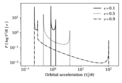
Figure 5 shows the orbital acceleration as a function of orbital phase (represented by the eccentric anomaly) for three separate orbital eccentricities. These are each normalized by , so a value of unity corresponds to the circular equivalent acceleration. Low eccentricity orbits have accelerations very close to whereas the orbital accelerations increase (decrease) around periastron (apastron) for larger eccentricities. Orbits with exhibit a double-minima feature around apastron, as shown by the dot-dashed line in Figure 5.
Since binaries spend more time near apastron than near periastron, Equation 11 must be combined with a function quantifying the amount of time spent at each orbital phase, , to determine the typical orbital accelerations observed for a population of binaries. After combining, we find:
| (12) |
where the summation is over the separate eccentric anomalies, , between 0 and corresponding to a given combination of , , and . For orbits with , Figure 5 shows that two solutions are possible, while as many as four solutions are available for orbits with . A closed-form solution does not exist for , so Equation 12 must be solved numerically. Figure 6 shows this corresponding probability, again normalized by . As expected, for low eccentricities, orbital accelerations are typically found near the circular values; even for orbits with , orbital accelerations are within a factor of a few of their circular equivalents. However, since eccentric binaries spend more time near apastron, orbits with larger eccentricities have orbital accelerations somewhat smaller than their circular values. We note that the spikes in Figure 6 are caused by the term in the denominator of Equation 12 going to zero at periastron and apastron.
By convolving Equation 12 with a distribution of eccentricities, , we can obtain the typical orbital accelerations expected from observing a “snapshot” of a population of binaries, again expressed in terms of :
| (13) |
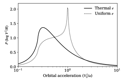
Figure 7 shows the resulting likelihoods of detecting orbital accelerations, normalized by , for two separate eccentricity distributions. For a uniform eccentricity distribution, , the distribution of orbital accelerations peaks strongly around the circular value, but with a significant tail with smaller values due to eccentric binaries being found near apocenter (). However, if we adopt a thermal eccentricity distribution, , the increased preference for binaries with higher eccentricities pushes the overall distribution toward smaller orbital accelerations. The resulting distribution peaks at the circular value ().
4 The Compact Object Population
4.1 Population Synthesis Predictions
We obtain an expectation for the number of BHs to be astrometrically observed by Gaia using binary population synthesis. For a complete description of the population generation parameters and astrophysical implications – including predictions for observability of astrometric binaries by Gaia – see Chawla et al. (in prep). Here, we describe the basic procedure, which is based on that presented in Breivik et al. (2019). We start by generating a population of initial stellar binaries with primary masses distributed according to Kroupa (2001) and secondary masses distributed uniformly with a binary fraction of . We assign each binary with an initial separation from a log-uniform distribution between a minimum value such that the system does not begin in Roche overflow and up to (Han, 1998). Finally, we assume that eccentricities are initially thermally distributed (Heggie, 1975).
While a complete description of the default parameters in COSMIC is provided by (Breivik et al., 2020), we highlight the most significant model prescriptions related to mass transfer and core collapse. Mass transfer stability is determined using the mass ratio conditions described in (Belczynski et al., 2008), with stable mass transfer following the procedure described in Hurley et al. (2002). We evolve binaries going through a common envelope using the prescription, where we set , corresponding to an efficient envelope ejection and is determined using the prescription described in the Appendix of Claeys et al. (2014). For stars going through core collapse, we follow the delayed prescription from Fryer et al. (2012). This prescription determines both the BH masses, as well as the amount of supernova ejecta that is accreted by the newly born BH as fallback mass. While BHs are initially given natal kicks drawn from a Maxwellian with km s-1, most BHs receive kicks close to or equal to zero, as fallback proportionally reduces the strength of the natal kick.
Those binaries that become BHs with luminous companions are then randomly sampled multiple times in its orbit at different eccentric anomalies and placing them in different locations throughout the Milky Way so the rates match the star formation rate, metallicity, and stellar density of the m12i galaxy in the Latte suite of the FIRE-2 simulation (Wetzel et al., 2016; Hopkins et al., 2018).
Finally, for each binary we calculate the apparent acceleration of the luminous object following Equation 11. We then sample 50 random Milky Way iterations to take into account the effects from stochastic sampling. Our procedure additionally includes two major improvements over the populations presented in Breivik et al. (2019): whereas Breivik et al. (2019) focused on giant stars, we account for all types of luminous companions, and we further include a dust model to account for extinction depending on each synthetic star’s position in the Milky Way.
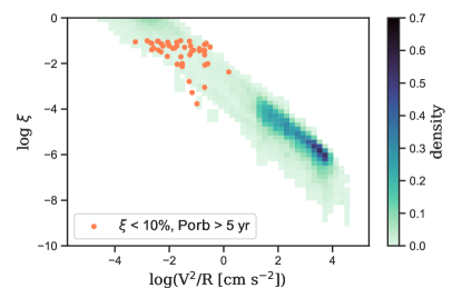
From our sample of synthetic binaries, Figure 8 compares the distribution of orbital accelerations with the measurement precision of Gaia on those accelerations. Contours are generated from 50 random Milky Way iterations and show the distribution of all systems comprised of a BH and a luminous star. Our simulations predict a large sample of binaries with ; these systems have orbital periods much less than 5 yrs and are therefore the subject of Paper I (the value of derived from Equation 7 is an extrapolation). The results in this work are relevant for systems with binary periods 5 years. After restricting for systems with an acceleration precision 0.1, 5 years, and a Gaia magnitude 20, we find Gaia ought to detect 47 such systems. We highlight in Figure 8 the systems generated by one particular Milky Way realization that satisfy these observability constraints (orange markers). While our 47 expected systems are derived from 50 random Milky Way realizations, we find 31 detectable systems in this particular example.
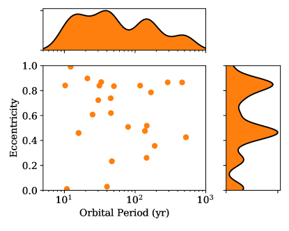
In Figure 9, we provide the log and for the same example Milky Way realization. The top and right panels provide one-dimensional histograms of log and , from which we see there is a preference for shorter systems and a slight preference for higher systems. Importantly, systems span the entire eccentricity range, and there is no clear cutoff at large . This suggest that a future instrument even more sensitive than Gaia would be able to detect systems at even larger .
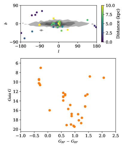
In Figure 10, we further describe the observational characteristics of the binaries in our synthetic Milky Way realization. In the top panel, we show the Galactic coordinates of these binaries (circular markers), with the marker colors indicating the distance to each system. A large fraction of systems are found near the center of the Milky Way, at distances of several kpc. Grayscale contours indicate the positions of a random sample of Gaia EDR3 stars, suggesting that many of these sources will be found in crowded fields. However, a number of nearby (1 kpc) systems exist far from the Milky Way center. The bottom panel shows that the luminous companions to the BHs in our sample of binaries span a wide range of magnitudes and Gaia colors. The brightest of these are accessible to even relatively small science-grade telescopes for observational follow-up.
4.2 Uniquely Identifying Compact Object Companions
Although our simulations suggest that Gaia is sensitive to 47 long-period binaries with BH companions, degeneracies prevent some binaries from being uniquely identified; the small acceleration produced by a massive BH companion in a long-period orbit, can also be caused by a low-mass, late-type star in somewhat shorter-period orbit. From Equation 8 the degeneracy can be expressed as .
How then to uniquely identify systems containing BH companions? In many cases such identification may not be possible. For binaries sufficiently close-by, follow-up observations with adaptive optics techniques may be able to resolve faint, low-mass companions in wide orbits. Yet even with the non-detection of a companion using state-of-the-art techniques and large aperture telescopes, a “lighter” companion in an even smaller orbit could also account for the observed acceleration. However, there is a mass limit below which the orbital period is too small to explain the observed acceleration; for small companions with sufficiently short orbital periods, Gaia ought to see a complete orbit over its lifetime (or at least measure a higher-order “jerk” term in the star’s motion). The fact that Gaia observes only part of an orbit sets a lower limit on the mass of a putative companion. Combining Equation 8 with the generalized form of Kepler’s Third Law, and replacing with twice Gaia’s lifetime (we assume an upper limit on the orbital period can be placed if at least half the orbit is observed) we find a relation between the two stars’ masses and the acceleration of the luminous star:
| (14) |
Note that we have assumed a circular orbit in deriving Equation 14, a point we address at the end of this section.
Combining the mass constraints from Equation 14 with high-angular-resolution follow-up imaging of any star showing large accelerations allow for the compact object nature of putative companions to be confirmed. Even faint white dwarf companions can be identified using this method.
For some systems, with Gaia alone, a non-degenerate companion can be ruled out by placing the limit , since the more massive star is the brighter of the two444Exceptions to this may exist for evolved companions, but such systems are rare.. Applying this limit to Equation 14, we find a limit on the luminous star’s mass:
| (15) |
For systems satisfying this constraint that do not complete a full orbit over Gaia’s lifetime, the observed acceleration may be due to a dark companion more massive than the observed star. A luminous companion cannot simultaneously produce the observed acceleration, be less luminous than the primary, and not complete a full orbit over Gaia’s lifetime. However, in such cases, a BH companion cannot be automatically assumed, as other exotic combinations may be possible (for instance the unseen companion could itself be a binary, that is faint, but with a substantial combined mass). We can only speculate that such systems will also be rare, and may themselves be astrophysically interesting (and therefore worthy of observational follow-up). Applying this limit to our population synthesis predictions, we find 15 of the 47 BH binaries can be identified as having dark compact objects555Note that depending on the system, both neutron star and BH companions may be possible; however we consider the detection of even one such system, regardless of whether it contains a neutron star or BH, to be a significant contribution to the study of compact object binaries..
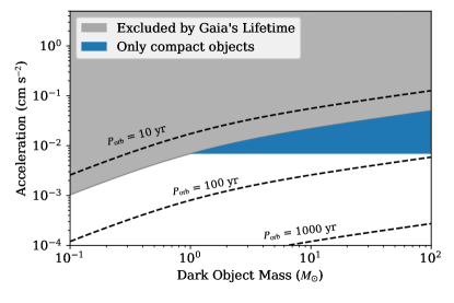
Figure 11 demonstrates the acceleration on a 1 luminous star caused by a companion object, as a function of its mass. We assume that for orbits with periods smaller than 20 years, Gaia will observe enough of the orbit to attempt a full fit. For longer period orbits, dark, massive companions are one possibility that can produce sufficiently large orbital accelerations (blue region).
We note that the relative orientation of an individual system ought to be irrelevant since the projected acceleration is always less than the total 3D acceleration. Therefore, any individual system identified as hosting a BH due to its high acceleration cannot be confused with a lower-mass, non-degenerate star in a circular orbit viewed at an inclined angle.
It is also worth considering contamination by non-faint companions. Since the luminosity of a Main Sequence star scales with , even slightly less-massive companions will contribute little to the overall luminosity of the system. However, for binaries with near-unity mass ratios, Gaia observes the motion of the photocenter of the system, rather than the more luminous star. The derivation of system parameters for such astrometric binaries was explored in a series of papers in the context of Hipparcos observations (Martin et al., 1997; Martin & Mignard, 1998; Martin et al., 1998). An extension of this concept to Gaia is outside the scope of this work and has been addressed elsewhere (Penoyre et al., 2020). Here, we only comment that for unresolved stars of equal magnitude, the binary’s photocenter will not display orbital motion. For stars with slightly differing masses, the photocenter moves, but the apparent acceleration is always smaller than that felt by the more massive star. Therefore our constraints defined in Equations 14 and 15 are unaffected by the possibility of luminous companions.
Finally, we note that the limits described in Equations 14 and 15 are derived assuming circular binaries. However, our analysis in Section 3 demonstrates that an eccentric binary at periastron produces a somewhat larger acceleration than its circular equivalent. While there is a distinct possibility that faint companions could produce the acceleration observed in any individual system identified using Equations 14 and 15 as hosting a dark, compact companion, Figure 6 shows that the chances of any one binary comprised of two luminous stars appearing to host a black hole are quite small; a small tail exists towards large accelerations (corresponding to the binary at periastron), but eccentric binaries typically show smaller orbital accelerations than their circular equivalent. However, binaries comprised of two luminous stars are common, while black hole binaries are extremely rare. We leave a comparative analysis determining the relative rates of the two populations to a future work.
5 Discussion and Conclusions
Although many previous studies have focused on the measurement of astrometric binaries by Gaia, nearly all focus on either systems in which Gaia observes at least one complete orbit or how Gaia data can be combined with other astrometric and spectroscopic data of known systems. According to Gaia’s data release scenario666https://www.cosmos.esa.int/web/gaia/release, the next data release (DR3) will contain information on astrometric binaries. Many of these will be systems with complete orbital solutions; however this data is also expected to contain a catalog of stars showing non-linear proper motions – orbital accelerations. In this work, we seek to broaden the family of binaries relevant for Gaia, by quantifying orbital accelerations in binaries with periods longer than Gaia’s lifetime. By fitting synthetic data using a Markov-Chain Monte Carlo method, we derive fitting formula that can be used to quantify Gaia’s ability to measure the orbital acceleration of any particular long-period binary. Depending on its distance, we find Gaia can measure orbital accelerations as small as cm s-2.
We then calculate the barycentric orbital acceleration as a function of orbital phase for eccentric binaries in Section 3. We find that inclination effects due to the orientation of the binary’s orbital plane are generally negligible. After combining with the length of time a binary spends at different orbital phases and a uniform distribution of eccentricities, we show in Figure 7 that orbits typically have accelerations comparable to, but somewhat smaller than, their circular equivalent. For a thermal eccentricity distribution, the orbital accelerations are typically a factor of 3 smaller.
For any individual system the observed acceleration is a function of the mass of the unknown companion and the orbital separation, a degeneracy which precludes a detailed fit for any individual system. However, populations of binaries ought to produce observable signals in the distribution. For example, if one knows the distribution of orbital separations of a population of long-period binaries, the distribution of companion masses can be derived from a Gaia sample of orbital accelerations. Or alternatively, a distribution of orbital separations can be derived if the distribution of companion masses is known. Again, eccentricity and inclination generally have only minor effects (and produce the same mean effect on all binaries anyway) so can be ignored at first order.
We then use binary population synthesis in Section 4 to generate a realistic population of BH binaries using our current best knowledge of binary evolution physics. After producing a sample of binaries and randomly placing them throughout the Milky Way according to a distribution and rate consistent with detailed evolution models of our Galaxy, we find that Gaia ought to observe 47 accelerating stars with BH companions. However, most of these systems are unlikely to be uniquely identified by Gaia. The degeneracy between mass and orbital separation means the same acceleration produced by any individual BH could also be produced by a faint, low-mass star with a smaller orbital separation. Nevertheless, for sufficiently small separations, Gaia will observe a complete orbit during its lifetime; if Gaia only sees an incomplete arc for a particular star, a lower limit on the companion mass can be derived. Using our binary population synthesis, we estimate that 15 BH binaries have sufficiently high lower limits on the companion masses that they can be unambiguously identified as hosting compact object companions.
These estimates are produced under the assumption of one particular parameterization of binary evolution. In Breivik et al. (2019), we demonstrate that the population of astrometric binaries containing a BH depends strongly on which parameters we choose to adopt; in that work, we focused on two separate BH mass functions from Fryer et al. (2012). Although we do not explicitly compare the two different prescriptions here, each will certainly affect the resulting yield of detached BH systems that Gaia will detect. A clear example for the case at present comes from how we model the kicks that BHs receive at birth. We adopt a model in which BH natal kicks are reduced due to fallback. For sufficiently massive BHs, these natal kicks become irrelevant; a 10 BH with an orbital separation of 10 au around a luminous star has an orbital velocity of 30 km s-1. However, if we adopt a model in which BHs receive a somewhat larger kick, similar in magnitude or larger at birth, a fraction of these will disrupt, reducing Gaia’s yield. Although a detailed comparison to different population synthesis prescriptions is outside the scope of this work, the case of BH kicks serves as an example which demonstrates, at least in principle, how a population of wide-period BH binaries can be used to constrain uncertain binary evolution physics.
Since the latest data release from Gaia (DR2) does not contain information about stellar binaries, the current best sample of stars with measured accelerations is that from Brandt (2018), who compares the proper motions from Gaia to that from HIPPARCOS. With its 24-year baseline, for stars detected by HIPPARCOS this catalog forms an excellent resource. Our scaling with time baseline in Equation 6 shows that sources detected by Gaia alone, with its 10-year lifetime, will have a factor of 6 degradation in acceleration measurement. However, this is more than made up for by the factor of improvement in Gaia’s astrometric precision over its predecessor; our simple estimate suggests that Gaia will be able to measure astrometric accelerations a factor of 20 better than has been possible previously, and for stars. Therefore, the 105 stars in the catalog from Brandt (2018) represent the tip of a much larger iceberg soon to be available.
References
- Hip (1997) 1997, ESA Special Publication, Vol. 1200, The HIPPARCOS and TYCHO catalogues. Astrometric and photometric star catalogues derived from the ESA HIPPARCOS Space Astrometry Mission
- Abdul-Masih et al. (2020) Abdul-Masih, M., Banyard, G., Bodensteiner, J., et al. 2020, Nature, 580, E11
- Andrews et al. (2015) Andrews, J. J., Agüeros, M. A., Gianninas, A., et al. 2015, ApJ, 815, 63
- Andrews et al. (2019a) Andrews, J. J., Anguiano, B., Chanamé, J., et al. 2019a, ApJ, 871, 42
- Andrews et al. (2019b) Andrews, J. J., Breivik, K., & Chatterjee, S. 2019b, ApJ, 886, 68
- Andrews et al. (2017) Andrews, J. J., Chanamé, J., & Agüeros, M. A. 2017, MNRAS, 472, 675
- Andrews et al. (2018) —. 2018, MNRAS, 473, 5393
- Astropy Collaboration et al. (2018) Astropy Collaboration, Price-Whelan, A. M., Sipőcz, B. M., et al. 2018, AJ, 156, 123
- Belczynski et al. (2008) Belczynski, K., Kalogera, V., Rasio, F. A., et al. 2008, ApJS, 174, 223
- Belokurov et al. (2020) Belokurov, V., Penoyre, Z., Oh, S., et al. 2020, MNRAS, 496, 1922
- Brandt (2018) Brandt, T. D. 2018, ApJS, 239, 31
- Brandt et al. (2018) Brandt, T. D., Dupuy, T. J., & Bowler, B. P. 2018, arXiv e-prints, arXiv:1811.07285
- Breivik et al. (2019) Breivik, K., Chatterjee, S., & Andrews, J. J. 2019, ApJ, 878, L4
- Breivik et al. (2017) Breivik, K., Chatterjee, S., & Larson, S. L. 2017, ApJ, 850, L13
- Breivik et al. (2020) Breivik, K., Coughlin, S., Zevin, M., et al. 2020, ApJ, 898, 71
- Cantat-Gaudin et al. (2018) Cantat-Gaudin, T., Jordi, C., Vallenari, A., et al. 2018, A&A, 618, A93
- Claeys et al. (2014) Claeys, J. S. W., Pols, O. R., Izzard, R. G., Vink, J., & Verbunt, F. W. M. 2014, A&A, 563, A83
- El-Badry & Quataert (2020) El-Badry, K., & Quataert, E. 2020, MNRAS, 493, L22
- El-Badry & Rix (2018) El-Badry, K., & Rix, H.-W. 2018, MNRAS, 480, 4884
- Eldridge et al. (2020) Eldridge, J. J., Stanway, E. R., Breivik, K., et al. 2020, MNRAS, 495, 2786
- Falin & Mignard (1999) Falin, J. L., & Mignard, F. 1999, A&AS, 135, 231
- Foreman-Mackey et al. (2013) Foreman-Mackey, D., Hogg, D. W., Lang, D., & Goodman, J. 2013, PASP, 125, 306
- Fryer et al. (2012) Fryer, C. L., Belczynski, K., Wiktorowicz, G., et al. 2012, ApJ, 749, 91
- Gaia Collaboration et al. (2016) Gaia Collaboration, Prusti, T., de Bruijne, J. H. J., et al. 2016, A&A, 595, A1
- Gaia Collaboration et al. (2018) Gaia Collaboration, Brown, A. G. A., Vallenari, A., et al. 2018, A&A, 616, A1
- Gaia Collaboration et al. (2019) Gaia Collaboration, Eyer, L., Rimoldini, L., et al. 2019, A&A, 623, A110
- Giesers et al. (2018) Giesers, B., Dreizler, S., Husser, T.-O., et al. 2018, MNRAS, 475, L15
- Giesers et al. (2019) Giesers, B., Kamann, S., Dreizler, S., et al. 2019, A&A, 632, A3
- Han (1998) Han, Z. 1998, MNRAS, 296, 1019
- Heggie (1975) Heggie, D. C. 1975, Mon. Not. R. Astron. Soc., 173, doi:10.1093/mnras/173.3.729
- Hopkins et al. (2018) Hopkins, P. F., Wetzel, A., Kereš, D., et al. 2018, MNRAS, 480, 800
- Hunt et al. (2018) Hunt, J. A. S., Hong, J., Bovy, J., Kawata, D., & Grand, R. J. J. 2018, MNRAS, 481, 3794
- Hunter (2007) Hunter, J. D. 2007, Computing in Science Engineering, 9, 90
- Hurley et al. (2002) Hurley, J. R., Tout, C. A., & Pols, O. R. 2002, MNRAS, 329, 897
- Jayasinghe et al. (2021) Jayasinghe, T., Stanek, K. Z., Thompson, T. A., et al. 2021, MNRAS, 504, 2577
- Jones et al. (2001) Jones, E., Oliphant, T., Peterson, P., et al. 2001, SciPy: Open source scientific tools for Python, , . http://www.scipy.org/
- Kervella et al. (2019) Kervella, P., Arenou, F., Mignard, F., & Thévenin, F. 2019, A&A, 623, A72
- Kroupa (2001) Kroupa, P. 2001, Mon. Not. R. Astron. Soc., 322, doi:10.1046/j.1365-8711.2001.04022.x
- Langer et al. (2020) Langer, N., Schürmann, C., Stoll, K., et al. 2020, A&A, 638, A39
- Lindegren et al. (2018) Lindegren, L., Hernández, J., Bombrun, A., et al. 2018, A&A, 616, A2
- Liu et al. (2019) Liu, J., Zhang, H., Howard, A. W., et al. 2019, Nature, 575, 618
- Martin & Mignard (1998) Martin, C., & Mignard, F. 1998, A&A, 330, 585
- Martin et al. (1997) Martin, C., Mignard, F., & Froeschle, M. 1997, A&AS, 122, 571
- Martin et al. (1998) Martin, C., Mignard, F., Hartkopf, W. I., & McAlister, H. A. 1998, A&AS, 133, 149
- Mashian & Loeb (2017) Mashian, N., & Loeb, A. 2017, MNRAS, 470, 2611
- Mason et al. (2001) Mason, B. D., Hartkopf, W. I., Holdenried, E. R., & Rafferty, T. J. 2001, AJ, 121, 3224
- Oelkers et al. (2017) Oelkers, R. J., Stassun, K. G., & Dhital, S. 2017, AJ, 153, 259
- Oh et al. (2017) Oh, S., Price-Whelan, A. M., Hogg, D. W., Morton, T. D., & Spergel, D. N. 2017, AJ, 153, 257
- Penoyre et al. (2020) Penoyre, Z., Belokurov, V., Wyn Evans, N., Everall, A., & Koposov, S. E. 2020, MNRAS, 495, 321
- Perryman et al. (1997) Perryman, M. A. C., Lindegren, L., Kovalevsky, J., et al. 1997, A&A, 500, 501
- Pittordis & Sutherland (2018) Pittordis, C., & Sutherland, W. 2018, MNRAS, 480, 1778
- Raghavan et al. (2010) Raghavan, D., McAlister, H. A., Henry, T. J., et al. 2010, ApJS, 190, 1
- Rivinius et al. (2020) Rivinius, T., Baade, D., Hadrava, P., Heida, M., & Klement, R. 2020, A&A, 637, L3
- Shahaf et al. (2019) Shahaf, S., Mazeh, T., Faigler, S., & Holl, B. 2019, arXiv e-prints, arXiv:1905.08542
- Shikauchi et al. (2020) Shikauchi, M., Kumamoto, J., Tanikawa, A., & Fujii, M. S. 2020, PASJ, 72, 45
- Snellen & Brown (2018) Snellen, I. A. G., & Brown, A. G. A. 2018, Nature Astronomy, 2, 883
- Thompson et al. (2019) Thompson, T. A., Kochanek, C. S., Stanek, K. Z., et al. 2019, Science, 366, 637
- Torres (2019) Torres, G. 2019, ApJ, 883, 105
- van der Walt et al. (2011) van der Walt, S., Colbert, S. C., & Varoquaux, G. 2011, Computing in Science Engineering, 13, 22
- van Leeuwen (2007) van Leeuwen, F. 2007, A&A, 474, 653
- Wetzel et al. (2016) Wetzel, A. R., Hopkins, P. F., Kim, J.-h., et al. 2016, ApJ, 827, L23
- Wiktorowicz et al. (2020) Wiktorowicz, G., Lu, Y., Wyrzykowski, Ł., et al. 2020, arXiv e-prints, arXiv:2006.08317
- Yalinewich et al. (2018) Yalinewich, A., Beniamini, P., Hotokezaka, K., & Zhu, W. 2018, MNRAS, 481, 930
- Yamaguchi et al. (2018) Yamaguchi, M. S., Kawanaka, N., Bulik, T., & Piran, T. 2018, ApJ, 861, 21
- Yi et al. (2019) Yi, T., Sun, M., & Gu, W.-M. 2019, ApJ, 886, 97