Velocity-imaging the rapidly precessing planetary disc around the white dwarf HE 1349–2305 using Doppler tomography

Abstract

The presence of planetary material in white dwarf atmospheres, thought to be accreted from a dusty debris disc produced via the tidal disruption of a planetesimal, is common. Approximately five per cent of these discs host a co-orbital gaseous component detectable via emission from atomic transitions – usually the 8600 Å Ca ii triplet. These emission profiles can be highly variable in both morphology and strength. Furthermore, the morphological variations in a few systems have been shown to be periodic, likely produced by an apsidally precessing asymmetric disc. Of the known gaseous debris discs, that around HE 1349–2305 has the most rapidly evolving emission line morphology, and we present updated spectroscopy of the Ca ii triplet of this system. The additional observations show that the emission line morphologies vary periodically and consistently, and we constrain the period to two aliases of 459 $\pm$ 3 d and 502 $\pm$ 3 d. We produce images of the Ca ii triplet emission from the disc in velocity space using Doppler tomography – only the second such imaging of a white dwarf debris disc. We suggest that the asymmetric nature of these velocity images is generated by gas moving on eccentric orbits with radially-dependent excitation conditions via photo-ionisation from the white dwarf. We also obtained short-cadence ($\simeq$ 4 min) spectroscopy to search for variability on the time-scale of the disc’s orbital period ($\simeq$ hours) due to the presence of a planetesimal, and rule out variability at a level of $\simeq$ 1.4 per cent.

1 Introduction

The observational evidence of planetary systems around white dwarfs is abundant (Zuckerman & Becklin, 1987; Graham et al., 1990; Aannestad et al., 1993; Vanderburg et al., 2015; Gänsicke et al., 2019; Manser et al., 2019; Vanderbosch et al., 2020; Vanderburg et al., 2020; Guidry et al., 2021; Vanderbosch et al., 2021). To date, the majority of detections of planetary material at white dwarfs have come from identifying pollutant metals in their atmospheres - the result of accreting planetary material (rocky planetesimals Zuckerman et al. 2003, 2010; Koester et al. 2014, icy Kuiper-belt analogues Xu et al. 2017, and even giant planet atmospheres Barstow et al. 2014; Gänsicke et al. 2019; Schreiber et al. 2019), with $\simeq$ 50 per cent of white dwarfs showing evidence of hosting remains of planetary systems. The majority of detections are thought to involve planetesimals that are assumed to have been perturbed onto highly eccentric orbits ($e>0.98$) by more massive bodies in the system (Debes & Sigurdsson, 2002), bringing them within the tidal disruption radius of the white dwarf ($\simeq$ 1 $\mathrm{R}_{\odot}$). The planetesimal is then ripped apart, forming a highly eccentric debris stream that is assumed to circularise within the tidal disruption radius to form a disc of dusty debris (Jura, 2003; Debes et al., 2012; Veras et al., 2014, 2015; Malamud & Perets, 2020a, b). These debris discs are usually detected via their infrared emission which is in excess of the white dwarf continuum (Zuckerman & Becklin, 1987; Rocchetto et al., 2015; Farihi, 2016; Chen et al., 2020; Dennihy et al., 2020a; Dennihy et al., 2020b; Gentile Fusillo et al., 2021; Xu et al., 2020).

Five per cent of infrared-bright debris discs around white dwarfs are observed to host an additional gaseous component in emission (Gänsicke et al., 2006; Manser et al., 2020), identified via the double-peaked Ca ii 8600 Å triplet emission profiles produced by a flat, photo-ionised Keplerian disc (Horne & Marsh, 1986; Melis et al., 2010; Kinnear, 2011; Gänsicke et al., 2019). The origin of these gaseous components is uncertain, but current mechanisms include: runaway sublimation of dust at the inner edge of the debris disc due to angular momentum conservation (Rafikov, 2011; Metzger et al., 2012), a collisional cascade of rocky bodies being ground down into dust and gas (Kenyon & Bromley, 2017a, b), collisions produced via a tidal stream of planetary debris impacting on a pre-existing disc (Jura, 2008; Malamud et al., 2021), and a disc-embedded planetesimal that survived the tidal disruption process, inducing the production of gas through collisions or sublimation (Manser et al., 2019; Trevascus et al., 2021). Recent observations show that variability of the infrared excess from debris discs is common (Xu & Jura, 2014; Xu et al., 2018; Swan et al., 2019; Wang et al., 2019), and it has been proposed that the observed variations are due to the production and destruction of dust via planetesimal collisions which could also produce observable gaseous material (Farihi et al., 2018; Swan et al., 2021). This is further corroborated by the discovery that debris discs with a gaseous component in emission appear to show the largest amounts of infrared variability (Swan et al., 2020), indicating they are the most dynamically active white dwarf debris discs. Henceforth we refer to dusty debris discs that have an additional, co-orbital gaseous component in emission as ‘gaseous debris discs’.

The gaseous emission profiles encode velocity information within the disc which provides insight into its dynamical structure. Long-term observations of the Ca ii triplet profiles show similar morphological variations of the emission profiles (Gänsicke et al., 2008; Melis et al., 2010; Wilson et al., 2015; Manser et al., 2016b; Dennihy et al., 2020b; Gentile Fusillo et al., 2021), which have been well-modelled for the disc around SDSS J122859.93+104032.9 (hereafter SDSS J1228+1040) using Doppler tomography (Marsh & Horne, 1988; Manser et al., 2016a). This modelling showed that the observed variability can be reproduced by the precession of a fixed, asymmetric intensity pattern in the disc on a period of $\simeq$ 27 yr. This is in agreement with theoretical studies which have shown that eccentric gas discs around white dwarfs should precess (with no radial dependence) due to a combination of general relativistic precession and gas pressure forces (Miranda & Rafikov, 2018).

HE 1349–2305 is a white dwarf of spectral type DBAZ (Koester et al., 2005), with an atmosphere dominated by helium harbouring trace amounts of hydrogen, as well as trace metals ingested from a debris disc that is detected as an infrared excess (Girven et al., 2012). The disc around HE 1349–2305 also hosts a gaseous component that appears to vary in a similar manner to SDSS J1228+1040, albeit with a tentative period of just 1.4 $\pm$ 0.2 yr (511 $\pm$ 73 d) (Melis et al., 2012; Dennihy et al., 2018). This period is an order-of-magnitude shorter than that of the disc around SDSS J1228+1040 (which has not yet been observed for a single full precession cycle), and gives us the opportunity to study the variability of these discs over multiple cycles to establish whether this period is stable. We note that the gaseous material around the white dwarf WD 1145+017 has been modelled as an eccentric disc that precesses with a period of 4.6 yr (Cauley et al., 2018; Fortin-Archambault et al., 2020), however this gaseous component is only detected via absorption and shows no evidence of emission.

In this manuscript we extend the $\simeq$ 0.95 yr of spectroscopy of the gaseous debris disc around HE 1349–2305 presented by Dennihy et al. (2018) by $\simeq$1.84 yr, covering now a total of $\simeq$ 2 cycles, in addition to two archival observation obtained in 2009 and 2011. We reanalyse the variability of the Ca ii triplet using both a time series analysis of their velocity centroids, and Doppler tomography confirming the disc is undergoing apsidal precession. We also inspect $\simeq$ 4 min cadence spectroscopy acquired to search for short-term variability due to the presence of a planetesimal. Finally, we discuss the results and the prospects of using Doppler maps as key probes in understanding the structure and evolution of gaseous debris discs.

2 Observations

The observations presented in this section were obtained from five observatories with the goal of monitoring the Ca ii triplet. The observations are documented in Table 1, and details of the instruments and telescopes used are given below.

Table 1: Log of HE 1349–2305 observations. The exposure times for the UVB/VIS arms of X-shooter are given separately.

Date	MJD [d]	Telescope/Instrument	Wavelength range [Å]	Total exposure time [s]	Resolution [Å]
2009-05-20	54971.2	Magellan/MIKE	3350 – 9500	1400	0.3
2011-05-27	55708.0	VLT/X-shooter	3080 – 10 400	5900 / 5680	1.0
2016-08-21	57621.0	SOAR/Goodman	7900 – 9000	7500	2.2
2017-01-12	57765.3	SOAR/Goodman	7900 – 9000	3600	2.2
2017-01-25	57778.4	SOAR/Goodman	7900 – 9000	3600	2.2
2017-02-05	57789.0	GTC/OSIRIS	7350 – 10 150	1800	2.5
2017-02-09	57793.3	SOAR/Goodman	7900 – 9000	3600	2.2
2017-02-17	57801.3	SOAR/Goodman	7900 – 9000	8400	2.2
2017-03-10	57822.2	SOAR/Goodman	7900 – 9000	5400	2.2
2017-03-14	57826.2	SOAR/Goodman	7900 – 9000	3600	2.2
2017-04-11a	57854.2	SOAR/Goodman	7900 – 9000	5400	2.2
2017-04-11b	57854.3	SOAR/Goodman	7900 – 9000	7200	2.2
2017-04-23	57866.2	SOAR/Goodman	7900 – 9000	3600	2.2
2017-05-30	57903.0	SOAR/Goodman	7900 – 9000	7200	2.2
2017-06-09	57913.1	SOAR/Goodman	7900 – 9000	7800	2.2
2017-07-25	57959.0	SOAR/Goodman	7900 – 9000	5400	2.2
2017-08-02	57968.0	SOAR/Goodman	7900 – 9000	6600	2.2
2018-02-04	58153.3	SOAR/Goodman	7900 – 9000	5400	2.2
2018-02-10	58159.3	SOAR/Goodman	7900 – 9000	4200	2.2
2018-03-27	58204.3	SOAR/Goodman	7900 – 9000	3600	2.2
2018-04-27	58235.3	SOAR/Goodman	7900 – 9000	5400	2.2
2018-05-15	58253.2	VLT/X-shooter	3080 – 10 400	2950 / 2840	1.0
2018-06-02	58271.1	SOAR/Goodman	7900 – 9000	9000	2.2
2019-03-09	58551.3	Gemini South/GMOS-S	8260 – 8790	9840	3.0
2019-03-16	58558.2	Gemini South/GMOS-S	8260 – 8790	10 800	3.0
2019-03-24	58566.2	SOAR/Goodman	7900 – 9000	7200	2.2
2019-04-23	58596.1	SOAR/Goodman	7900 – 9000	6000	2.2
2019-05-15	58618.2	SOAR/Goodman	7900 – 9000	7200	2.2
2019-06-06	58640.1	VLT/X-shooter	3080 – 10 400	2950 / 2840	1.0

Southern Astrophysical Research (SOAR) Telescope/Goodman High Throughput Spectrograph (Goodman): Goodman is a highly configurable low resolution spectrograph mounted on the SOAR 4m telescope (Clemens et al., 2004). The data were collected using the 1200l-R grating and were reduced using a custom set of python-based tools described in (Dennihy et al., 2018), utilising an optimal extraction routine based on the methods described in Marsh (1989).

Very Large Telescope (VLT)/X-shooter: X-shooter is an intermediate resolution echelle spectrograph on the ESO VLT (Vernet et al., 2011). The data (program IDs: 087.D-0858(A), 5100.C-0407(C), and 5100.C-0407(I)) were reduced within the reflex  reduction work flow using the standard settings and optimising the slit integration limits (Freudling et al., 2013), and a telluric correction was performed using molecfit (Smette et al., 2015; Kausch et al., 2015). The 2019 June spectrum is shown in Fig. 1, where the NIR arm of X-shooter was not used due to low counts in the infrared.

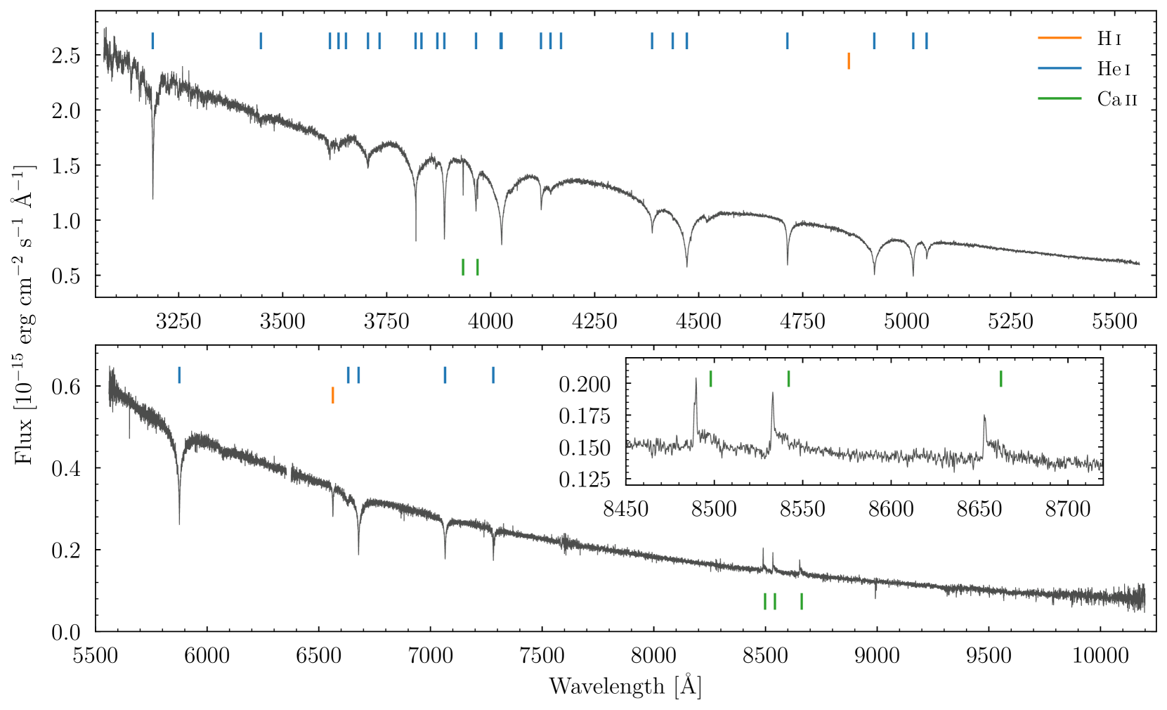
Figure 1: The 2019 June X-shooter spectrum of HE 1349–2305. The inset shows a zoom-in of the Ca ii triplet region, revealing a blue-dominated circumstellar emission feature, with little red-shifted material in emission implying a strongly asymmetric brightness distribution in the disc. The coloured tabs denote the rest wavelengths of strong H, He, and Ca features; only the lowest two energy transitions of the Balmer series are detected.

Magellan/Magellan Inamori Kyocera Echelle (MIKE): The MIKE spectrograph on the Magellan telescope is a double-echelle spectrograph capable of high resolution over a wide wavelength range (Bernstein et al., 2003). The data were reduced and extracted using the Carnegie python tools MIKE data reduction pipeline, with methodology described in Kelson (2003).

Gran Telescopio Canarias (GTC)/Optical System for Imaging and low-Intermediate-Resolution Integrated Spectroscopy (OSIRIS): HE 1349–2305 was observed at the 10.4 m GTC on 2017 Feburary 5 using the OSIRIS spectrograph with the volume-phased holographic R2500I grating (program ID: GTC1-16ITP). The observations were reduced using standard techniques under the starlink software package. The science frames were bias-subtracted and flat-fielded, and sky-subtraction and extraction of the 1-D spectra were performed using the pamela software package, where the optimal-extraction algorithm was used to maximise the spectral signal-to-noise ratio. The molly package was used for wavelength calibration of the extracted 1-D data.

Gemini South/Gemini Multi-Object Spectrograph (GMOS-S): GMOS-S on Gemini South is a highly configurable instrument capable of multi-object, longslit and integral-field unit spectroscopy (Hook et al., 2004; Gimeno et al., 2016). The data were collected using the R-831 grating (program ID: S-2019A-Q-231). The data were reduced using a combination of the Gemini iraf package and an optimal extraction routine based on the methods described in Marsh (1989). We obtained a total of 86, 4 min exposures (totalling 20640 s) on 2019 March 9 (41 exposures) and 16 (45 exposures) to search for any short-term variations in the emission strength and morphology of the Ca ii triplet on the time-scale of the orbital period in the disc ($\simeq$ hours).

3 Gaseous emission profiles

The characteristic emission profile from a circular gaseous disc of gas on Keplerian orbits with a radially symmetric intensity distribution is a symmetric, double-peaked emission profile (see fig.1 of Horne & Marsh 1986). These profiles can reveal structural properties of the disc such as the inner and outer radii. The inner radius of such a disc can be determined by the velocity at which the emission drops to the continuum level of the spectrum, and the absolute velocity between the blue- and red-shifted sides of the profile is known as the full width zero intensity (FWZI). A FWZI not centered at 0 km s^-1 is indicative of an asymmetry in the disc, and may be due to a non-symmetric emitting area in a circular disc (e.g. spiral shocks, Steeghs & Stehle 1999), or a non-circular disc geometry (e.g. eccentric discs, Fortin-Archambault et al. 2020). The outer radius of a circular disc in emission can be estimated from the peak separation of the double-peaked profile, but is also affected by disc asymmetries which can lead to differences in the positions and strengths of the two peaks. This type of asymmetry is clearly evident in the emission profiles of HE 1349–2350 (Fig. 1), where only one emission peak is evident. The radii estimates, $R_{\textrm{obs}}$ obtained through these methods are affected by the inclination, $i$ of the disc, and to determine the true radii, $R$, one must use $R_{\textrm{obs}}=R\sin^{2}i$. We use this insight to discuss the line profiles observed at HE 1349–2305.

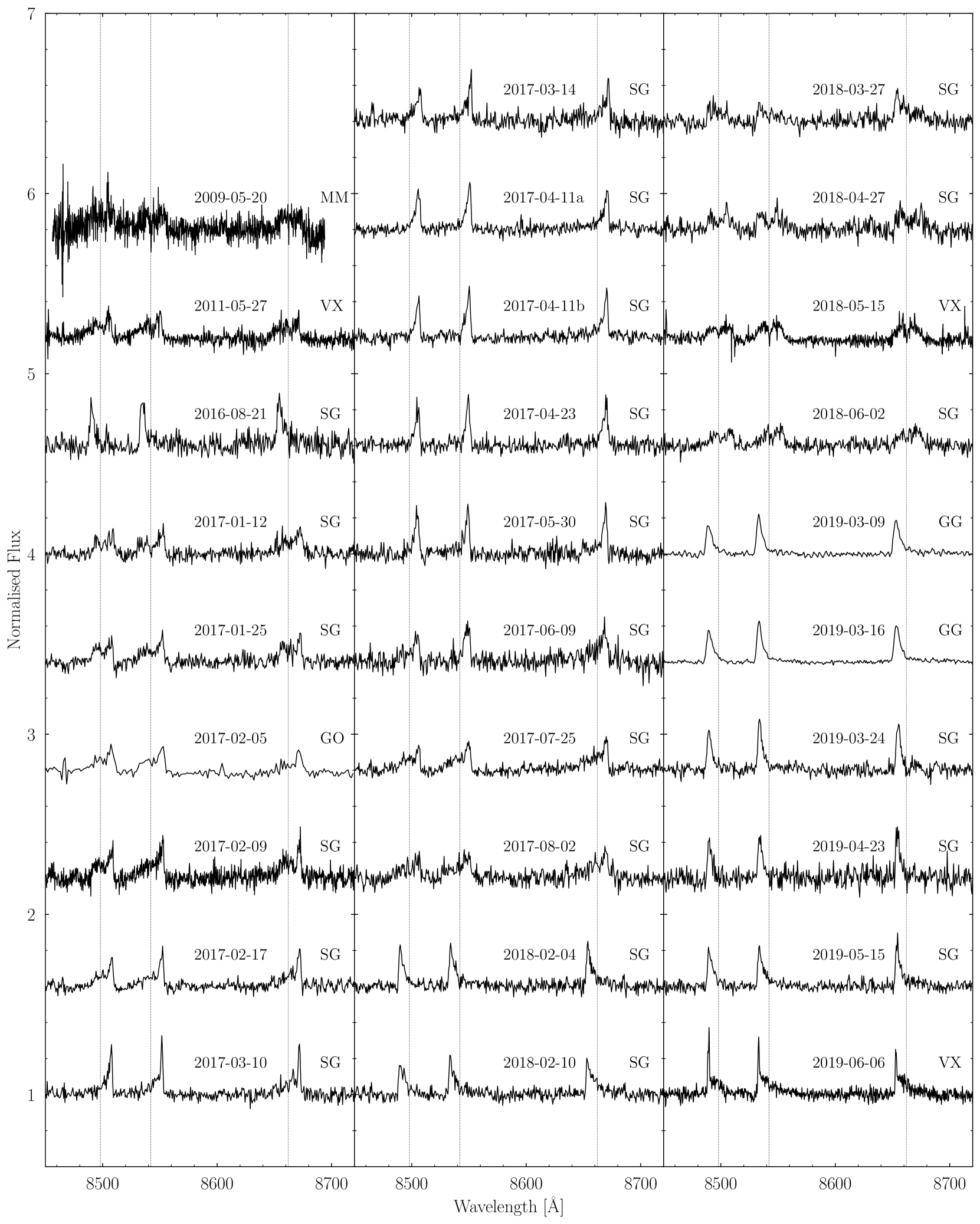
Figure 2: Continuum-normalised spectra of the Ca ii triplet emission from the gaseous component of the debris disc around HE 1349–2305. The epochs of the 29 spectra are given along with a two letter code using the first initial of the telescope and instrument used for the observation, see Table 1. The spectra are shifted in the $y$-axis by steps of 0.6 from a value of one for clarity, and vertical dashed lines correspond to the rest wavelengths of the triplet components.

The Ca ii triplet emission from the disc around HE 1349–2305 is undergoing morphological variability as shown by the emission profiles in Fig. 2, where the spectra are continuum-normalised in the wavelength range 8450 – 8720 Å. We have extended the intense monitoring of the Ca ii triplet of Dennihy et al. (2018) from 2018 February to 2019 June with twelve additional spectra, which confirm the continued variation of the emission profiles (Fig. 2). Below we analyse the morphological variations of the Ca ii triplet using two methods: (i) Velocity centroid fitting, and (ii) Doppler tomography.

3.1 Velocity centroid fitting of the Ca ii triplet

Table 2: Log of velocity centroids given for each component of the Ca ii.

		Ca ii 8498 Å	Ca ii 8542 Å	Ca ii 8662 Å
Date	MJD [d]	Velocity centroid [km s-1]
2011-05-27	55708.0	7 $\pm$ 24	–8 $\pm$ 19	–21 $\pm$ 15
2016-08-21	57621.0	–218 $\pm$ 34	–215 $\pm$ 29	–215 $\pm$ 30
2017-01-12	57765.3	156 $\pm$ 52	122 $\pm$ 81	160 $\pm$ 62
2017-01-25	57778.4	95 $\pm$ 77	15 $\pm$ 55	102 $\pm$ 50
2017-02-05	57789.0	158 $\pm$ 27	193 $\pm$ 45	207 $\pm$ 49
2017-02-09	57793.3	107 $\pm$ 46	92 $\pm$ 45	167 $\pm$ 77
2017-02-17	57801.3	144 $\pm$ 33	251 $\pm$ 62	180 $\pm$ 72
2017-03-10	57822.2	202 $\pm$ 56	257 $\pm$ 19	253 $\pm$ 28
2017-03-14	57826.2	256 $\pm$ 41	232 $\pm$ 44	258 $\pm$ 65
2017-04-11a	57854.2	229 $\pm$ 21	246 $\pm$ 19	247 $\pm$ 25
2017-04-11b	57854.3	204 $\pm$ 31	247 $\pm$ 82	235 $\pm$ 25
2017-04-23	57866.2	223 $\pm$ 19	207 $\pm$ 28	227 $\pm$ 23
2017-05-30	57903.0	197 $\pm$ 17	207 $\pm$ 21	195 $\pm$ 24
2017-06-09	57913.1	208 $\pm$ 31	86 $\pm$ 62	161 $\pm$ 47
2017-07-25	57959.0	64 $\pm$ 42	42 $\pm$ 55	64 $\pm$ 41
2017-08-02	57968.0	143 $\pm$ 65	80 $\pm$ 56	92 $\pm$ 139
2018-02-04	58153.3	–216 $\pm$ 30	–208 $\pm$ 31	–204 $\pm$ 38
2018-02-10	58159.3	–180 $\pm$ 44	–204 $\pm$ 43	–184 $\pm$ 24
2018-03-27	58204.3	–122 $\pm$ 72	–60 $\pm$ 67	–66 $\pm$ 98
2018-04-27	58235.3	69 $\pm$ 142	71 $\pm$ 125	133 $\pm$ 72
2018-05-15	58253.2	82 $\pm$ 34	96 $\pm$ 35	86 $\pm$ 26
2018-06-02	58271.1	139 $\pm$ 115	136 $\pm$ 60	136 $\pm$ 60
2019-03-09	58551.3	–269 $\pm$ 18	–274 $\pm$ 9	–256 $\pm$ 20
2019-03-16	58558.2	–272 $\pm$ 9	–251 $\pm$ 9	–261 $\pm$ 10
2019-03-24	58566.2	–271 $\pm$ 23	–212 $\pm$ 23	–231 $\pm$ 39
2019-04-23	58596.1	–244 $\pm$ 30	–263 $\pm$ 57	–239 $\pm$ 45
2019-05-15	58618.2	–216 $\pm$ 32	–219 $\pm$ 28	–233 $\pm$ 20
2019-06-06	58640.1	–164 $\pm$ 23	–274 $\pm$ 27	–151 $\pm$ 26

The velocity centroid method relies on measuring the flux-weighted average velocity of the emission profiles as they oscillate between blue- and red-dominated phases. We follow the same methods as outlined in Dennihy et al. (2018) to measure the velocity centroid for each emission profile at every epoch (Table 2), excluding the 2009 May MIKE spectrum from the analysis as its average signal-to-noise ratio of $\simeq$ 13 is not sufficient for velocity centroiding. The velocity centroids for the Ca ii triplet profiles were then averaged at each epoch and the resulting time-series velocity centroids were analysed using the analysis of variance (ANOVA) method, which is particularly powerful in the case of unevenly sampled data (see Schwarzenberg-Czerny, 1996, for details). The resulting periodogram is shown in Fig. 3, which reveals two clear peaks in frequency at (2.18 $\pm$ 0.01) $\times$10^-3 d^-1 and (1.99 $\pm$ 0.01) $\times$10^-3 d^-1 corresponding to periods of 459 $\pm$ 3 d (1.257 $\pm$ 0.008 yr) and 502 $\pm$ 3 d (1.374 $\pm$ 0.009 yr) respectively. Due to the $\simeq$ 0.4 – 1 yr gaps present in our data collection, we cannot distinguish between these two period-aliases. We phase-fold the epoch-averaged velocity centroid data on these two periods (Fig. 3), to illustrate the periodic nature of the variations. Both of the periods are shorter than, but consistent with, the previously determined period of 511 $\pm$ 73 d.

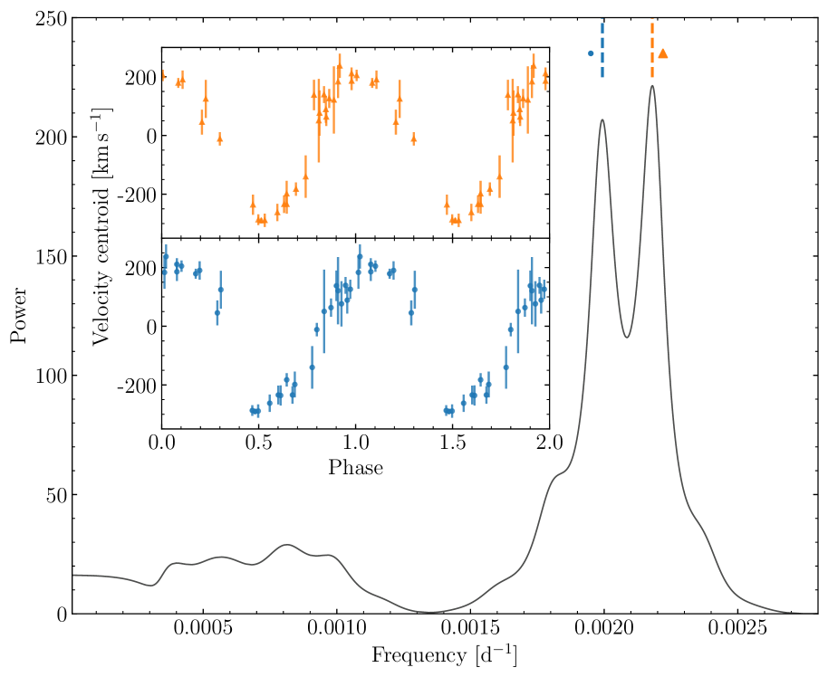
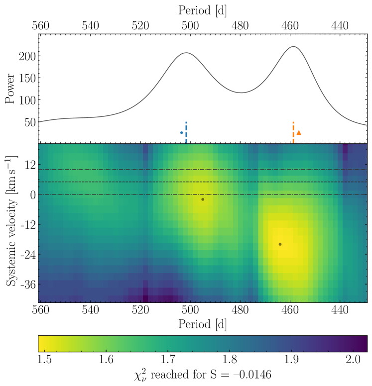
Figure 3: Left: The periodogram calculated using the ANOVA method (see text) of the triplet-averaged velocity centroids of the profiles in Fig. 2 displays two distinct peaks at periods 459 $\pm$ 3 d (orange triangle) and 502 $\pm$ 3 d (blue circle). The inset shows the velocity centroids phase-folded onto the two periods using the same colours and symbols. Right: The top panel reproduces a section of the periodogram presented in the left panel in period space. The bottom panel shows the $\chi^{2}_{\nu}$, for Doppler tomograms reached at an entropy, $S$ = $-0.0146$, for a range of precession periods and systemic velocities. Lower values signify better fits, with two local minima denoted by black dots. The dashed line shows the systemic velocity determined by Melis et al. (2012), and the dot-dashed lines depict a lower limit on the $\pm$ 1 $\sigma$ region.

3.2 Doppler tomography of the Ca ii triplet

Doppler tomography uses the one-dimensional velocity information encapsulated in the emission profiles to produce a two-dimensional image of the disc in velocity space – known as a Doppler tomogram or Doppler map. This technique relies on several assumptions: (1) That all points on the disc are equally visible at all times. (2) The flux from any point fixed in the rotating frame is constant in time. (3) All motion is parallel to the orbital plane. (4) The intrinsic width of the profile from any point is negligible (Marsh, 2001). As these tomograms are usually made for a specific group of atomic transitions, one can use these to map the location of multiple emitting species (Unda-Sanzana et al., 2006). To determine whether the disc around HE 1349–2305 is also apsidally precessing with a fixed period, we compute Doppler maps for the system’s gaseous emission. This also allows for the period of variability of the system to be independently calculated for comparison with the velocity centroid analysis described above.

To generate a Doppler map with the 29 normalised spectra shown in Fig. 2 we fix two free parameters: the period, $P$, and systemic velocity, $\gamma$. We use the maximum entropy inversion method described in Marsh & Horne (1988) whereby for a given target reduced chi-squared $\chi^{2}_{\nu}$, the Doppler map with the highest entropy $S$ (or least information) is selected. As the target $\chi^{2}_{\nu}$ is reduced, the maximum value of $S$ will also decrease from a value of zero as a more complex structure in the Doppler map is required. As such, for a given value of $P$ and $\gamma$, a target $S$ can be selected and the corresponding map with the minimum $\chi^{2}_{\nu}$ can be determined. The exact value of $S$ is unimportant, and a choice of $S$ = –0.0146 (a dimensionless quantity) was selected based on preliminary Doppler map fits. We computed Doppler maps for a grid of $430$ $\textrm{d}\leq P\leq 560$ d in steps of 2 d and $-42\textrm{km\,s}^{-1}\leq\gamma\leq 20$km s^-1 in steps of 3 km s^-1, with the results shown in Fig. 3.

We identify two minima in our $P$-$\gamma$ grid with periods of 464 d and 494 d, with corresponding systemic velocities of $-21$ km s^-1 and $-3$ km s^-1, and we perform a finer grid search around these minima moving in steps of 1 d in $P$ and 1 km s^-1 in $\gamma$. The Doppler maps produced at these minima have periods of 464 d (1.27 yr) and 495 d (1.36 yr), with corresponding systemic velocities of $-20$ km s^-1 and $-2$ km s^-1 and $\chi^{2}_{\nu}$ of 1.492 and 1.528 respectively. The precession periods we determine are in agreement with those determined by the ANOVA analysis of the velocity centroids. We show the Doppler maps corresponding to periods of 464 d and 495 d in Fig. 4, and present the resulting fits from these maps to the Ca ii triplet emission profiles in Fig. 5. The maps look similar, with an extremely asymmetric intensity distribution with only one side of the disc showing emission. We note that while these intensity patterns are fixed in a frame of constant apsidal precession, the orbital period of the material in the disc ($\simeq$ hours) is orders of magnitude faster. The observed asymmetry is not unexpected from the emission profiles, where the most extreme epochs show the complete disappearance of one peak. For example, in 2017 April (2019 March) the blue(red)-shifted peak is not present. On both maps there are high velocity, low intensity regions of emission that are most likely artefacts arising from the assumptions of Doppler tomography being broken (see section 4.3 and fig. 6 of Marsh & Horne 1988 for examples), as they differ significantly between the two maps. Some of these can be seen at $v_{\textrm{y}}$ $<$ $-$250 km s^-1 in both maps, and also along $v_{\textrm{y}}$ $\simeq$ 250 km s^-1 in the 495 d period map.

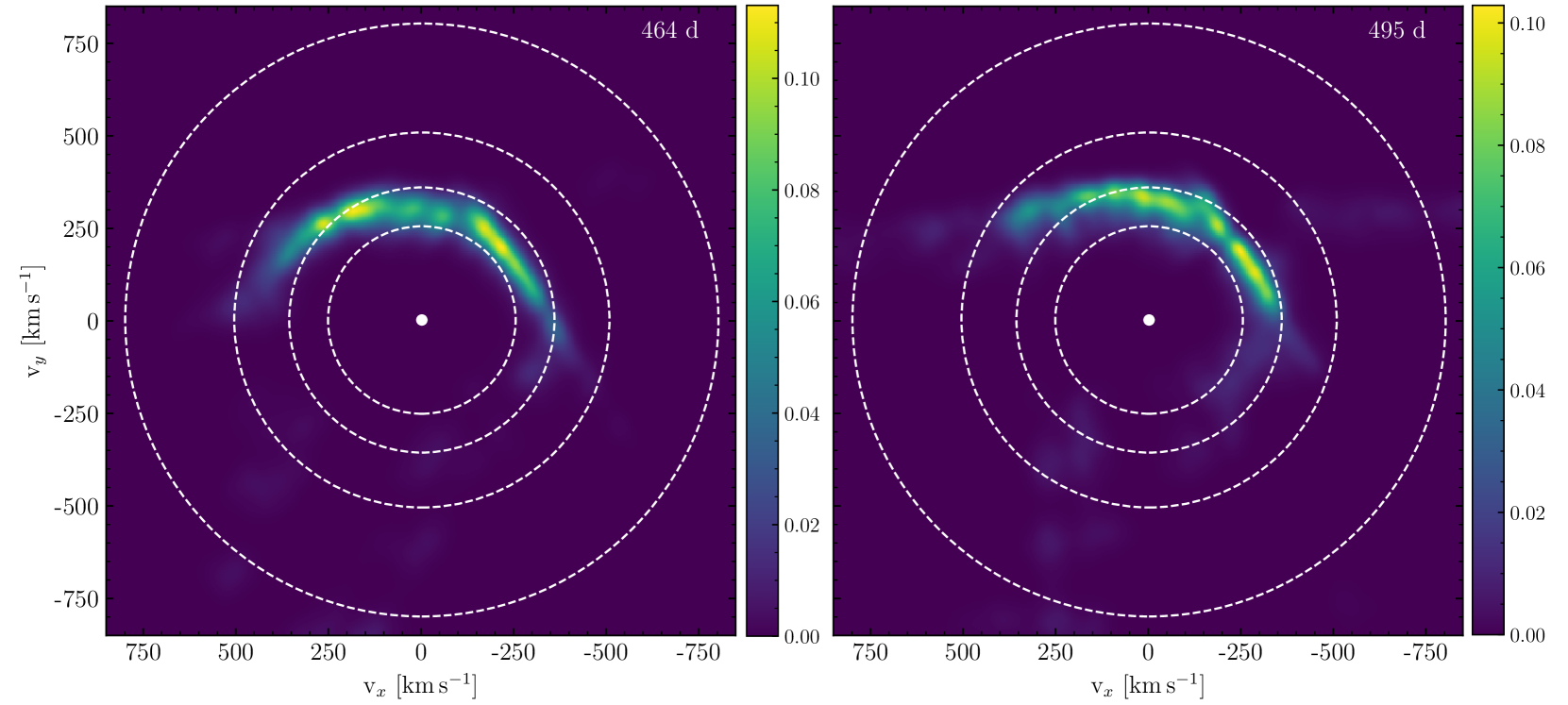
Figure 4: Doppler maps of the disc around HE 1349–2305 assuming a period of 464 d and a systemic velocity of $-20$ km s^-1 in the left panel, and a period of 495 d and a systemic velocity of $-2$ km s^-1 in the right panel. Circular orbits (white dashed lines) assuming the disc has an inclination, $i$ = 90 ${}^{\textrm{o}}$, and the white dwarf has a mass $M_{\textrm{WD}}$ = 0.673 $\mathrm{M}_{\odot}$ (Koester et al., 2005; Voss et al., 2007), are shown with radii 0.2, 0.5, 1.0, and 2.0 $\mathrm{R}_{\odot}$ in order from the largest circle to the smallest. The colour bar shows the brightness of the disc in arbitrary units.

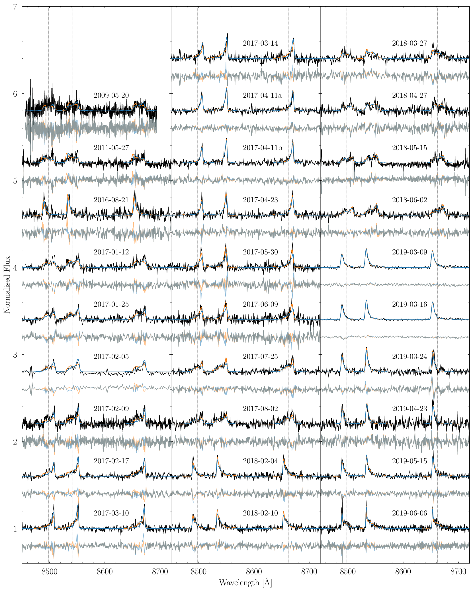
Figure 5: Comparison of the observed spectra of HE 1349–2305 and those generated from the fitted Doppler maps. The Ca ii triplet profiles (black) are shown with the profile fits generated from the 464 d (orange) and 495 d (blue) period Doppler maps presented in Fig. 4. The residuals for both fits are shown directly below each profile in orange and blue for the 464 d and 495 d periods respectively, with overlapping residuals presented in grey.

Inspecting the profile fits (Fig. 5) for both periods show that an apsidally precessing disc of fixed-intensity gives an excellent qualitative explanation for the variability we see, however there are epochs for both periods where the fits deviate from the line profiles. The majority of these deviations appear to be due to slight morphological differences in the fits resulting in shallow residual profiles (e.g. 2017 February 9), or small differences in the positions of the emission peak between the data and the fit, leading to large residual spikes (e.g. 2017 May 30 and 2019 March 24). The fits of the profiles produced by the 464 d period are worst in the earliest epochs, from 2009 May to 2017 March, after which the fits improve and are consistent over $\simeq$ 1.75 precession cycles. Comparatively the worst-fitted profiles for the 495 d map occur at 2009 May, 2011 May, and between 2017 March and 2017 July.

Both maps poorly fit the first two epochs in 2009 May and 2011 May - where in the latter the observed and fitted profiles appear in anti-phase for both maps. These spectra were not obtained as part of our dedicated monitoring, and are $\simeq$ 6 – 7 full precession cycles away from the most recent observation for both periods, and may suggest that, over multiple precession cycles, the assumptions of Doppler tomography requiring either the intensity pattern or the precession period of the disc to be constant breaks down. Similar morphological deviations of the fits are seen for SDSS J1228+1040 in fig. 7 of Manser et al. (2016a) for the first five years of data. Short-term variations (compared to the precession period of $\simeq$ 27 yr) were invoked to account for the deviations, which may be due to the recently observed presence of a disc-embedded planetesimal (Manser et al., 2019).

Due to the aliasing issues revealed by the velocity centroid analysis, the maps are very similar in both brightness and morphology, and it is not possible to reject a map based on their $\chi^{2}_{\nu}$ values alone. The systemic velocity has previously been estimated at $\gamma\simeq 5$ km s^-1 by Melis et al. (2012). The authors used data obtained by the Ultraviolet and Visual Echelle Spectrograph (UVES) on the VLT (Voss et al., 2007) to determine the velocity shift of photospheric absorption features in the white dwarf spectrum, found to be 40 $\pm$ 5 km s^-1, and subtracted from this an estimation of the gravitational red-shift due to the white dwarf of 35 km s^-1. We show this estimation of $\gamma$ on Fig. 3 with an error of $\pm$ 5 km s^-1 from the velocity shift determination. This error, however, does not take into account the uncertainty on the gravitational red-shift estimate used. As such, we cannot currently distinguish between the two consistent periods determined using either velocity centroids or Doppler tomography.

3.3 Additional candidate emission profiles

While the Ca ii triplet emission features were discovered and analysed in other works, we have identified subtle, candidate emission features at the 3934 Å Ca ii K, 5169 Å Fe ii (Fig. 6), and 8446 Å O i (Fig. 7) lines. While the 3934 Å Ca ii K feature is significantly weaker, the emission morphology appears to evolve between the two epochs from a symmetric profile to blue-shift dominated one, matching the morphological evolution of the Ca ii triplet emission. Furthermore, the velocity of the blue-shifted peak of the 2019 June Ca ii K profile of $-$320 $\pm$ 10 km s^-1 is consistent with that of the 2019 June Ca ii triplet profiles with an average of $-$307 $\pm$ 8 km s^-1. The candidate emission feature detected in the 5169 Å Fe ii region also changes in morphology between the two epochs, where the red-shifted component of the profile contracts to shorter wavelengths, corresponding to smaller velocities. We note that this region has also been shown to host 5167 Å, 5173 Å, and 5184 Å Mg i emission for some gaseous debris discs (see Melis et al. 2020; Dennihy et al. 2020b; Gentile Fusillo et al. 2021). The potential O i emission feature appears to share the red-dominated asymmetry of the Ca ii triplet.

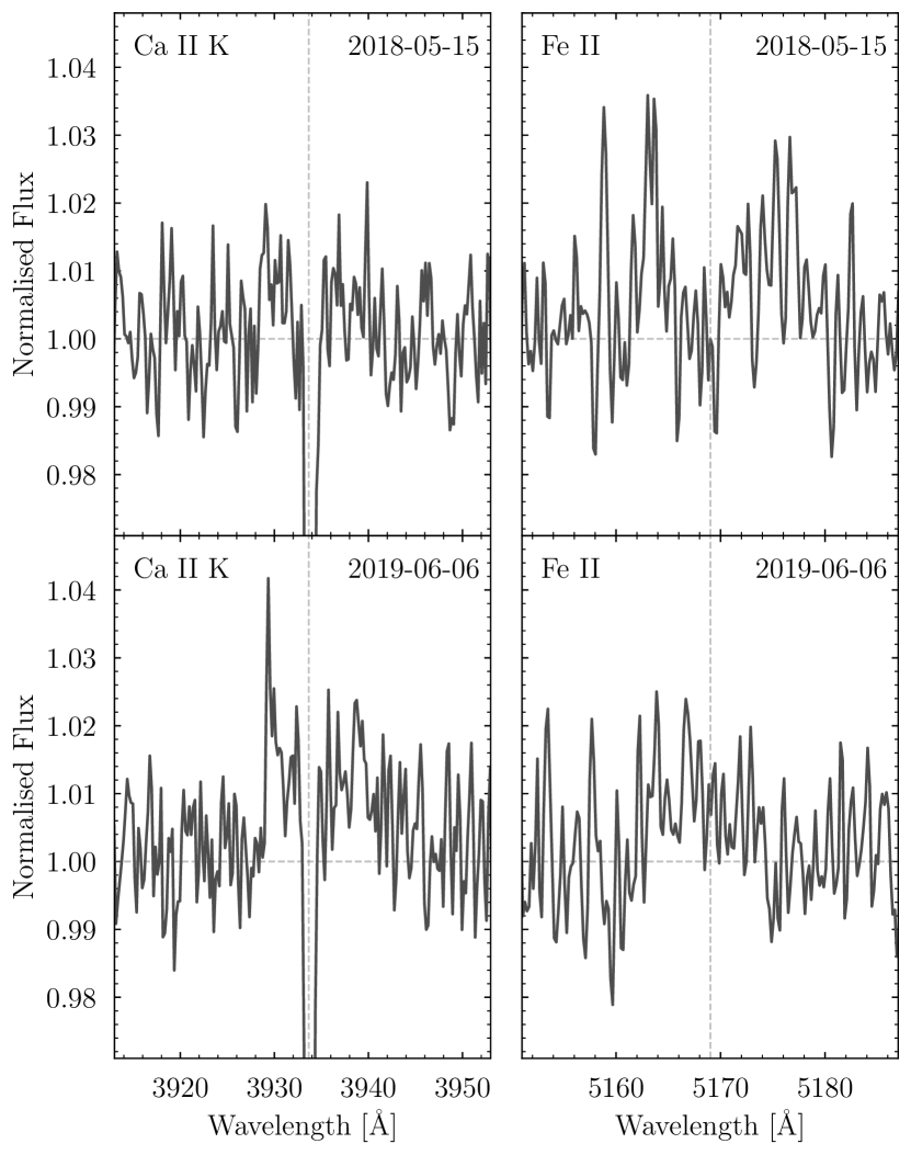
Figure 6: The 3934 Å Ca ii K and 5169 Å Fe ii regions of the 2018 and 2019 continuum-normalised X-shooter spectra. The absorption feature due to Ca ii K in the white dwarf photosphere is clearly present. Vertical dashed lines corresponding to zero-velocity air wavelengths of the Ca ii K and Fe ii transitions are presented for clarity.

Figure 7: The 8446 Å O i region bluewards of the Ca ii triplet reveals potential emission in the coadded continuum-normalised GMOS spectra. Vertical dashed lines corresponding to zero-velocity air wavelengths of the O i and Ca ii triplet transitions are presented for clarity.

While the candidate 3934 Å Ca ii K and 8446 Å O i features discovered at HE 1349–2305 appear to show morphologies consistent with the Ca ii triplet, this may not be the case for the 5169 Å Fe ii feature, and is not necessarily always true for emission lines formed by gaseous debris discs. The varied morphologies of different emission lines, both between atomic species and transitions of the same species, have been observed previously for other gaseous debris discs, most notably SDSS J1228+1040 (Manser et al., 2016a). It was speculated for the disc around SDSS J1228+1040 that the distribution of emitting ions in the disc may differ for a given atomic transition. However, additional high signal-to-noise ratio spectroscopy is needed to confirm the presence of the additional emission features identified in Figs 6 & 7 for the disc around HE 1349–2305.

4 Short-cadence observations of the Ca ii triplet

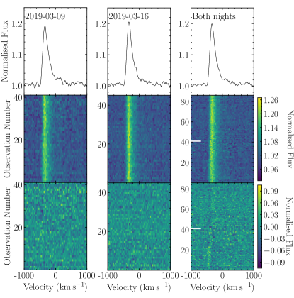
Figure 8: Short-cadence (4 min exposure time) GMOS spectra of the Ca ii triplet emission from the disc around HE 1349–2305, where the triplet profiles have been co-added in velocity space to boost the signal-to-noise ratio. The figures show data from 2019 March 09, 2019 March 16, and both nights combined in the respectively labelled figures. We assume the rest air-wavelength for each transition. The top panels show the Ca ii triplet profiles averaged over the time-resolved data shown in the middle panels as trailed spectrograms, where the Ca ii triplet emission profiles can be seen as vertical streaks. The white bars show the change from data taken on 2019 March 09 to 2019 March 16. By subtracting the the average spectra (top panels) from the trailed spectrograms (middle panels), the bottom panels are obtained showing the average-subtracted trailed spectrograms. No short-term variability is detected, however in the average-subtracted trailed spectrogram including both nights of data there is a subtle signature of the precession ($\simeq$ 5 ${}^{\textrm{o}}$) changing the morphology of the Ca ii triplet profiles between the two nights.

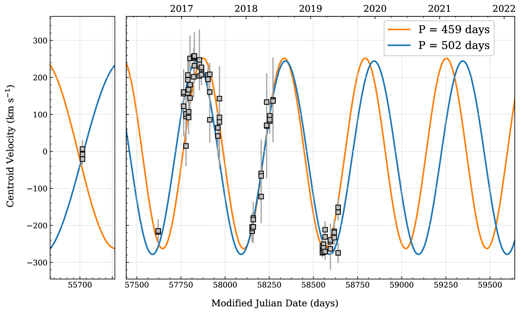
Figure 9: Sinusoidal fits to the velocity centroids of the Ca ii triplet profiles shown in Fig. 2, corresponding to periods of 459 d (orange) and 502 d (blue) obtained using the ANOVA method. Each observation (at a given time) is represented by three gray points (sometimes overlapping), corresponding to the three components of the Ca ii triplet. The $x$-axis is given in both Modified Julian date (bottom) and in calender year (top).

We obtained a total of 86, 4 min exposures (totalling 344 min, or 5.73 hr) on 2019 March 9 (41 exposures) and 16 (45 exposures) using the 8.1 m Gemini South telescope to search for any short-term variations in the emission strength and morphology of the Ca ii triplet on the time-scale of the orbital period in the disc ($\simeq$ hours). Periodic variations in the Ca ii triplet emission were observed at the debris disc around SDSS J1228+1040 and were found to be due to a planetesimal embedded in the disc with an orbital period of 123.4 min (Manser et al., 2019). HE 1349–2305 may host a disc-embedded planetesimal detectable through short-term periodic variations, however, the order of magnitude difference in the strength of the emission lines between SDSS J1228+1040 and HE 1349–2305 makes this a challenging task. If the level of emission produced by the short-term signal is proportional to the brightness of the Ca ii triplet lines, then the signal strength of $\simeq$ 10 per cent observed for SDSS J1228+1040 (e.g. fig. S4 of Manser et al. 2019) would correspond to an expected signal strength of $\lesssim$ 1 per cent for the emission lines at HE 1349–2305. The required signal-to-noise ratio to detect such a signal would be > 100.

We co-added the normalised spectra of all three Ca ii triplet components in velocity to boost the signal-to-noise ratio, and present trailed spectrograms in Fig. 8. The typical signal-to-noise ratio of the velocity spectra is $\simeq$ 70, and the single night data show no evidence of any short term variations in the emission ruling out short-term variability at a level of 1.4 per cent. If the expected short-term signal is proportional to the brightness of the Ca ii triplet then the quality of the data obtained is not sufficient to exclude the presence of a planetesimal similar to that around SDSS J1228+1040. We note that the trailed spectrogram combining both nights of data reveals very subtle variations in each of the Ca ii triplet profiles, which is a result of the apsidal precession of the debris disc between the two nights.

5 Discussion

We have presented updated monitoring of the long-term morphological variations seen in the emission profiles of HE 1349–2305 and analysed the period and systemic velocity measurements obtainable from this data. We also searched for short-term variations in the strength and shape of the line profiles on the order of hours to no avail.

5.1 Precession of the debris disc

The relatively short precession period of HE 1349–2305 makes this an ideal system for studying cycle-to-cycle stability. While SDSS J1228+1040 presents the strongest emission lines identified so far, it would take $\simeq$ 50 yr to cover two precession cycles.

While there appears to be some discrepancy in our fitting between early observations of HE 1349–2305 in 2009 and 2011, and the later monitoring between 2016 and 2019, the morphological variations expected for a fixed intensity pattern are well described by the Doppler maps shown in Fig 4. Additional spectroscopy of the Ca ii triplet profiles is required to resolve the aliasing in the periods of variability we determine. Fig. 9 shows sinusoidal curves with periods of 459 d and 502 d fit to the velocity centroid data, illustrating the drift between the two periods over time. By mid 2021 and beyond, the two periods will be separated enough that a single observation may be able to break the degeneracy, however this relies on the assumption that the apsidal precession has a fixed period. We therefore suggest that continued ($\simeq$ monthly) monitoring of this system over the next few years with high signal-to-noise ratio, moderate-resolution spectroscopy (resolving power R $\sim$ 10 000) is required to break the period degeneracy and search for any robust deviation from a constant period over multiple precession cycles.

A useful property that can be obtained from the Doppler map is the distribution of emitting gaseous debris in velocity space, which can be compared against disc models and expectations from hypothesised disc configurations. The disc around SDSS J1228+1040 is thought to be moderately eccentric ($e$ $\simeq$ 0.3-0.5), which is possibly generated by an embedded planetesimal. The eccentricity of the disc is likely driving the long-term precession through general relativistic precession and pressure forces (Miranda & Rafikov, 2018). The emission profiles around HE 1349–2305 appear significantly more asymmetric than those of SDSS J1228+1040, and along with the dramatically shorter precession period would indicate the disc is at least as eccentric as SDSS J1228+1040. For the 495 d period Doppler map, we plotted an eccentric orbit in velocity space shown in Fig. 10 using the equations described in Appendix A, which show that eccentric orbits are represented by circles in velocity space, offset from the origin with a displacement depending on $e$. The emission from the debris disc can be well described by an arc of an eccentric orbit, with the emission brighter at the apocentre of the orbit. We note that this is not a fit to the data, but a guide to the eye as a proof of concept, using an eccentricity, $e$ = 0.35, orbital period $P_{\textrm{orb}}$ = 60 min, a disc inclination, $i$ = 1 rad $\simeq$ 57.3 ${}^{\textrm{o}}$, and $M_{\textrm{WD}}$ = 0.673 $\mathrm{M}_{\odot}$ (Koester et al., 2005; Voss et al., 2007). The value of $i$ used here is the average value for the inclination of a randomly oriented disc given no information, and we use it here as an example. The pericentre value obtained for this set-up of $\simeq$ 0.24 $\mathrm{R}_{\odot}$ is loosely consistent with the findings of Miranda & Rafikov (2018). However, we refrain from drawing any definitive conclusions from this set-up given that multiple free parameters can be adjusted to obtain a similar fit (e.g. $e$ = 0.3, $P_{\textrm{orb}}$ = 120 min, $i$ = 90 ${}^{\textrm{o}}$).

Figure 10: The 495 d doppler map shown in Fig. 4 with an eccentric orbit (red) overplotted with $e$ = 0.35, orbital period $P_{\textrm{orb}}$ = 60 min, and an inclination, $i$ = 1 rad $\simeq$ 57.3 ${}^{\textrm{o}}$. We note that eccentric orbits are represented by offset circles in velocty space (see Appendix A). The white dashed lines show circular orbits with radii 0.2, 0.5, 1.0, and 2.0 $\mathrm{R}_{\odot}$ in order from the largest circle to the smallest, assuming the same inclination.

An interesting and simple consequence of gaseous material following an eccentric orbit is that the gas will be changing in radial distance from the white dwarf as it travels along the orbit. Photo-ionisation models show that the emission strength of a particular atomic species in a gaseous disc is dependent on the disc temperature (Melis et al. 2010; Kinnear 2011; Gänsicke et al. 2019, see also discussion of Gentile Fusillo et al. 2021) - itself dependent on the distance from the white dwarf (Steele et al., 2021). As this distance is varying throughout the eccentric orbit, we would expect the emission strength of the Ca ii triplet to change as well. For HE 1349–2305, it appears that the material is brightest at apocentre where the material has the lowest velocities in the map. This is consistent with SDSS J1228+1040, where the brightest part of the Ca ii triplet intensity distribution in the disc occurs in the lowest velocity region - around apocentre (fig. 5 of Manser et al. 2016a). This inverse correlation between emission strength and disc temperature has been observed in gaseous debris disc simulations, and is due to a shift in the ionisation balance of Ca ii/Ca iii (Hartmann et al., 2011, 2016), where photons of energy 11.87 eV or higher are required for ionisation of Ca ii (Ferland et al., 2017).

The scenario described above also explains why the different atomic species observed in the disc at SDSS J1228+1040 have very different profile shapes. The morphology of the O i emission from the disc at SDSS J1228+1040 is almost in anti-phase with the shape of the Ca ii triplet, which can be explained by O i emission arising from hotter material closer to pericentre (see also fig. 7.1 of Manser 2018). This is consistent with the upper energy levels that produce the $\simeq$7775 Å triplet and 8446 Å O i lines ($\simeq$ 10.74 eV and 10.99 eV respectively), requiring a hotter gas orbiting closer to the white dwarf than compared with the Ca ii triplet (upper energy levels of $\simeq$ 3.12-3.15 eV, Kramida et al. 2019). However, the potential O i emission we detect for HE 1349–2305 appears to share the morphology of the Ca ii triplet, suggesting they are being generated by gas in a similar location. A possible explanation for this is that given the potential for shorter orbital periods outlined above, the gaseous debris may be hotter around HE 1349–2305, and both Ca ii and O i are more readily ionised (O i has an ionisation energy of 13.62 eV) near the pericentre of the orbit and reducing the available ions for emission. However, this is largely speculation, and we have not taken into account the lower $T_{\textrm{eff}}$ of HE 1349–2305 (18 173 K, Melis et al. 2012) compared with that of SDSS J1228+1040 (20 713 K Koester et al. 2014). The production of Doppler maps (with a constant $\gamma$ and $P$) of multiple atomic species for a single gaseous debris disc would allow these postulates to be tested, as well as provide useful comparisons for models of the disc, such as those that have been produced using CLOUDY (Kinnear, 2011; Ferland et al., 2017; Gänsicke et al., 2019; Steele et al., 2021).

5.2 Non-detection of short-term periodic variations

We do not detect short-term variability due to the presence of a planetesimal, but cannot rule out variability below $\simeq$ 1.4 per cent. While reducing the uncertainty of future observations of HE 1349–2305 may help to rule out variability at a more significant level, it would require dedicated observations on an 8 - 10 meter class telescope over multiple nights. If the emission generated by a single planetesimal is proportional in strength to the total emission from the gaseous component of the disc, then it would be more efficient to observe gaseous debris discs with emission features comparable in strength to those at SDSS J1228+1040.

Melis et al. (2020), Dennihy et al. (2020b) and Gentile Fusillo et al. (2021) recently reported the combined detection of 14 new gaseous debris discs (for a total of 21 gaseous debris disc systems), five of which – SDSS J0006+2858, WD 0347+1624, WD 0611–6931, WD J0846+5703, and WD J2133+2428, show strong Ca ii triplet emission. Furthermore, the morphology of the emission profiles of WD 0347+1624 appears to vary on a time-scale of 2 - 3 yrs; similar to HE 1349–2305 and indicative of the precession of the debris disc. These systems are currently the best gaseous debris discs to probe in search of short-term variability on the time-scale of the orbital period in the disc induced by the presence of a single planetesimal.

While our discussion has focused on detecting the signal from a single planetesimal, it has been suggested that multiple planetesimals undergoing collisional cascades can explain the observed variability of the infrared components of white dwarf debris discs and their connection to gaseous emission (Swan et al., 2021). A debris disc hosting multiple planetesimals is not at odds with the detection of a single planetesimal at SDSS J1228+1040, as the majority of the mass in these discs are contained within the few largest bodies. Further research into the evolution of the gaseous component to white dwarf debris discs, the variability of the dusty infrared emission, and the survival of planetary bodies within the typically assumed Roche radius ($\simeq$ 1 $\mathrm{R}_{\odot}$) are required to refine these hypotheses.

6 Conclusions

We presented observations revealing continued morphological evolution of the emission from the gaseous debris disc around the white dwarf HE 1349–2305. The Ca ii triplet profiles are well fit by a fixed, asymmetric intensity pattern undergoing apsidal precession. While we have determined aliased periods that require future observations to distinguish, we show that they are consistent with previous analysis of the velocity centroids of the profiles. We also hypothesise that the asymmetric intensity distributions seen in Doppler maps of HE 1349–2305 and SDSS J1228+1040 are due to the radially dependant excitation conditions as the gas moves on eccentric orbits around the photo-ionising white dwarf.

We find no evidence of short-term variability on the orbital time-scale of the disc, which may have indicated the presence of a planetesimal. However, if there is a correlation between the strength of the overall Ca ii triplet profile and any short-term signal, then our results are likely dominated by noise. Future observations of bright white dwarfs with strong emission from a gaseous debris disc, such as WD J0347+1624 or WD J0846+5703, would help to determine if this is the case.

Gaseous debris discs around white dwarfs show a remarkable range of variability, and the potential to Doppler map these apsidally precessing discs using Doppler tomography is still in its early stages. Additional monitoring of the now 21 known gaseous debris discs is critical in following any morphological evolution present, and to eventually produce Doppler maps of them using Doppler tomography. These Doppler maps, along with the plethora of emission signatures beyond the Ca ii triplet seen in some systems will be vital in determining fundamental parameters of these discs, such as their temperature and surface density profiles, and studying their dynamical evolution.

Data availability

All data underlying this article is publicly available from the relevant observatory archive (see program IDs in text) or will be shared on reasonable request to the corresponding author.

Appendix A Eccentric orbits in velocity space

One curious property of eccentric orbits in velocity space is that they are represented as offset circles, which was identified independently by both Möbius (1843) and Hamilton (1847), and has been discussed in numerous other works since (e.g., Cariñena et al. 2016 and references therein), where velocity diagrams are usually referred to as ‘hodographs’. We re-illustrate here that eccentric orbits can be represented as offset circles in velocity space using the formalism described in Appendix A of Manser et al. (2016b). We start with their equations A12-15:

$$v_{x}=v_{r}\cos f-v_{f}\sin f,$$ (1)

$$v_{y}=v_{r}\sin f+v_{f}\cos f,$$ (2)

$$v_{r}=\frac{el\sin f}{\left(1+e\cos f\right)^{2}}\,\frac{\textrm{d}f}{\textrm{d}t},$$ (3)

$$v_{f}=\frac{l}{1+e\cos f}\,\frac{\textrm{d}f}{\textrm{d}t},$$ (4)

where $v$ is the velocity, $e$ is the eccentricity, $f$ is the true anomaly, $l=a(1-e^{2})$ is the semi-latus rectum, $a$ is the semi-major axis, and $\frac{\textrm{d}f}{\textrm{d}t}$ is the derivative of the true anomaly with respect to time which can be written as

$$\frac{\textrm{d}f}{\textrm{d}t}=\frac{(1+e\cos f)^{2}}{\left(1-e^{2}\right)^{3/2}}n.$$ (5)

where $n=2\pi/P_{\textrm{orb}}$, and $P_{\textrm{orb}}$ is the orbital period. Substituting equation 5 into equations 3 & 4 results in

$$v_{r}=\frac{enl\sin f}{\left(1-e^{2}\right)^{3/2}},$$ (6)

$$v_{f}=\frac{nl(1+e\cos f)}{\left(1-e^{2}\right)^{3/2}}.$$ (7)

Substituting equations 6 & 7 into equations 1 & 2 and reducing gives

$$v_{x}=-\frac{nl\sin f}{\left(1-e^{2}\right)^{3/2}},$$ (8)

and

$$v_{y}=\frac{enl}{\left(1-e^{2}\right)^{3/2}}+\frac{nl\cos f}{\left(1-e^{2}\right)^{3/2}}.$$ (9)

Finally, by substituting,

$$K=\frac{nl}{\left(1-e^{2}\right)^{3/2}}=\frac{2\pi l}{P_{\textrm{orb}}\left(1-e^{2}\right)^{3/2}}=\frac{2\pi a}{P_{\textrm{orb}}\left(1-e^{2}\right)^{1/2}},$$ (10)

into equations 8 & 9, we get

$$v_{x}=-K\sin f,$$ (11)

and

$$v_{y}=Ke+K\cos f.$$ (12)

Equations 11 & 12 show that an eccentric orbit in velocity space is represented by a circle of radius $K$ and offset from the origin by $Ke$. $K$ can be modified easily to include the inclination, $i$ (given that $v_{\textrm{obs}}=v\sin i$), as,

$$K=\frac{2\pi a\sin i}{P_{\textrm{orb}}\left(1-e^{2}\right)^{1/2}},$$ (13)

and can be rewritten in terms of $P_{\textrm{orb}}$, $M_{\textrm{WD}}$, $e$, and $i$,

$$K=\left(\frac{2\pi GM_{\textrm{WD}}}{P_{\textrm{orb}}}\right)^{1/3}\frac{\sin i}{\left(1-e^{2}\right)^{1/2}},$$ (14)

where $G$ is the gravitational constant.

References

- Aannestad et al. (1993) Aannestad P. A., Kenyon S. J., Hammond G. L., Sion E. M., 1993, AJ, 105, 1033
- Barstow et al. (2014) Barstow M. A., Barstow J. K., Casewell S. L., Holberg J. B., Hubeny I., 2014, MNRAS, 440, 1607
- Bernstein et al. (2003) Bernstein R., Shectman S. A., Gunnels S. M., Mochnacki S., Athey A. E., 2003, in Iye M., Moorwood A. F. M., eds, Society of Photo-Optical Instrumentation Engineers (SPIE) Conference Series Vol. 4841, Proc. SPIE. pp 1694–1704, doi:10.1117/12.461502
- Cariñena et al. (2016) Cariñena J. F., Rañada M. F., Santander M., 2016, European Journal of Physics, 37, 025004
- Cauley et al. (2018) Cauley P. W., Farihi J., Redfield S., Bachman S., Parsons S. G., Gänsicke B. T., 2018, ApJ, 852, L22
- Chen et al. (2020) Chen C. H., Su K. Y. L., Xu S., 2020, Nature Astronomy, 4, 328
- Clemens et al. (2004) Clemens J. C., Crain J. A., Anderson R., 2004, in Moorwood A. F. M., Iye M., eds, Society of Photo-Optical Instrumentation Engineers (SPIE) Conference Series Vol. 5492, Proc. SPIE. pp 331–340, doi:10.1117/12.550069
- Debes & Sigurdsson (2002) Debes J. H., Sigurdsson S., 2002, ApJ, 572, 556
- Debes et al. (2012) Debes J. H., Walsh K. J., Stark C., 2012, ApJ, 747, 148
- Dennihy et al. (2018) Dennihy E., Clemens J. C., Dunlap B. H., Fanale S. M., Fuchs J. T., Hermes J. J., 2018, ApJ, 854, 40
- Dennihy et al. (2020a) Dennihy E., Farihi J., Fusillo N. P. G., Debes J. H., 2020a, ApJ, 891, 97
- Dennihy et al. (2020b) Dennihy E., et al., 2020b, ApJ, 905, 5
- Farihi (2016) Farihi J., 2016, New Astronomy Reviews, 71, 9
- Farihi et al. (2018) Farihi J., et al., 2018, MNRAS, 481, 2601
- Ferland et al. (2017) Ferland G. J., et al., 2017, Rev. Mex. Astron. Astrofis., 53, 385
- Fortin-Archambault et al. (2020) Fortin-Archambault M., Dufour P., Xu S., 2020, ApJ, 888, 47
- Freudling et al. (2013) Freudling W., Romaniello M., Bramich D. M., Ballester P., Forchi V., García-Dabló C. E., Moehler S., Neeser M. J., 2013, A&A, 559, A96
- Gänsicke et al. (2006) Gänsicke B. T., Marsh T. R., Southworth J., Rebassa-Mansergas A., 2006, Science, 314, 1908
- Gänsicke et al. (2008) Gänsicke B. T., Koester D., Marsh T. R., Rebassa-Mansergas A., Southworth J., 2008, MNRAS, 391, L103
- Gänsicke et al. (2019) Gänsicke B. T., Schreiber M. R., Toloza O., Fusillo N. P. G., Koester D., Manser C. J., 2019, Nature, 576, 61
- Gentile Fusillo et al. (2021) Gentile Fusillo N. P., et al., 2021, MNRAS, 504, 2707
- Gimeno et al. (2016) Gimeno G., et al., 2016, in Evans C. J., Simard L., Takami H., eds, Society of Photo-Optical Instrumentation Engineers (SPIE) Conference Series Vol. 9908, Ground-based and Airborne Instrumentation for Astronomy VI. p. 99082S, doi:10.1117/12.2233883
- Girven et al. (2012) Girven J., Brinkworth C. S., Farihi J., Gänsicke B. T., Hoard D. W., Marsh T. R., Koester D., 2012, ApJ, 749, 154
- Graham et al. (1990) Graham J. R., Matthews K., Neugebauer G., Soifer B. T., 1990, ApJ, 357, 216
- Guidry et al. (2021) Guidry J. A., et al., 2021, ApJ, 912, 125
- Hamilton (1847) Hamilton W. R., 1847, Proc. R. Ir. Acad., 3, 344
- Hartmann et al. (2011) Hartmann S., Nagel T., Rauch T., Werner K., 2011, A&A, 530, A7
- Hartmann et al. (2016) Hartmann S., Nagel T., Rauch T., Werner K., 2016, A&A, 593, A67
- Hook et al. (2004) Hook I. M., Jørgensen I., Allington-Smith J. R., Davies R. L., Metcalfe N., Murowinski R. G., Crampton D., 2004, PASP, 116, 425
- Horne & Marsh (1986) Horne K., Marsh T. R., 1986, MNRAS, 218, 761
- Jura (2003) Jura M., 2003, ApJ Lett., 584, L91
- Jura (2008) Jura M., 2008, AJ, 135, 1785
- Kausch et al. (2015) Kausch W., et al., 2015, A&A, 576, A78
- Kelson (2003) Kelson D. D., 2003, PASP, 115, 688
- Kenyon & Bromley (2017a) Kenyon S. J., Bromley B. C., 2017a, ApJ, 844, 116
- Kenyon & Bromley (2017b) Kenyon S. J., Bromley B. C., 2017b, ApJ, 850, 50
- Kinnear (2011) Kinnear T., 2011, Master’s thesis, University of Warwick
- Koester et al. (2005) Koester D., Rollenhagen K., Napiwotzki R., Voss B., Christlieb N., Homeier D., Reimers D., 2005, A&A, 432, 1025
- Koester et al. (2014) Koester D., Gänsicke B. T., Farihi J., 2014, A&A, 566, A34
- Kramida et al. (2019) Kramida A., Yu. Ralchenko Reader J., and NIST ASD Team 2019, NIST Atomic Spectra Database (ver. 5.7.1), [Online]. Available: https://physics.nist.gov/asd [2020, September 2]. National Institute of Standards and Technology, Gaithersburg, MD.
- Malamud & Perets (2020a) Malamud U., Perets H. B., 2020a, MNRAS, 492, 5561
- Malamud & Perets (2020b) Malamud U., Perets H. B., 2020b, MNRAS, 493, 698
- Malamud et al. (2021) Malamud U., Grishin E., Brouwers M., 2021, MNRAS, 501, 3806
- Manser (2018) Manser C. J., 2018, PhD thesis, University of Warwick
- Manser et al. (2016a) Manser C. J., et al., 2016a, MNRAS, 455, 4467
- Manser et al. (2016b) Manser C. J., Gänsicke B. T., Koester D., Marsh T. R., Southworth J., 2016b, MNRAS, 462, 1461
- Manser et al. (2019) Manser C. J., et al., 2019, Science, 364, 66
- Manser et al. (2020) Manser C. J., Gänsicke B. T., Gentile Fusillo N. P., Ashley R., Breedt E., Hollands M., Izquierdo P., Pelisoli I., 2020, MNRAS, 493, 2127
- Marsh (1989) Marsh T. R., 1989, PASP, 101, 1032
- Marsh (2001) Marsh T. R., 2001, in Boffin H. M. J., Steeghs D., Cuypers J., eds, Lecture Notes in Physics, Berlin Springer Verlag Vol. 573, Astrotomography, Indirect Imaging Methods in Observational Astronomy. p. 1 (arXiv:astro-ph/0011020)
- Marsh & Horne (1988) Marsh T. R., Horne K., 1988, MNRAS, 235, 269
- Melis et al. (2010) Melis C., Jura M., Albert L., Klein B., Zuckerman B., 2010, ApJ, 722, 1078
- Melis et al. (2012) Melis C., et al., 2012, ApJ Lett., 751, L4
- Melis et al. (2020) Melis C., Klein B., Doyle A. E., Weinberger A., Zuckerman B., Dufour P., 2020, ApJ, 905, 56
- Metzger et al. (2012) Metzger B. D., Rafikov R. R., Bochkarev K. V., 2012, MNRAS, 423, 505
- Miranda & Rafikov (2018) Miranda R., Rafikov R. R., 2018, ApJ, 857, 135
- Möbius (1843) Möbius A. F., 1843, Die Elemente der Mechanik des Himmels: auf neuem Wege ohne Hülfe höherer Rechnungsarten. Weidmannsche Buchhandlung, Leipzig
- Rafikov (2011) Rafikov R. R., 2011, MNRAS, 416, L55
- Rocchetto et al. (2015) Rocchetto M., Farihi J., Gänsicke B. T., Bergfors C., 2015, MNRAS, 449, 574
- Schreiber et al. (2019) Schreiber M. R., Gänsicke B. T., Toloza O., Hernandez M.-S., Lagos F., 2019, ApJ, 887, L4
- Schwarzenberg-Czerny (1996) Schwarzenberg-Czerny A., 1996, ApJ Lett., 460, L107
- Smette et al. (2015) Smette A., et al., 2015, A&A, 576, A77
- Steeghs & Stehle (1999) Steeghs D., Stehle R., 1999, MNRAS, 307, 99
- Steele et al. (2021) Steele A., Debes J., Xu S., Yeh S., Dufour P., 2021, ApJ, 911, 25
- Swan et al. (2019) Swan A., Farihi J., Wilson T. G., 2019, MNRAS, 484, L109
- Swan et al. (2020) Swan A., Farihi J., Wilson T. G., Parsons S. G., 2020, MNRAS, 496, 5233
- Swan et al. (2021) Swan A., Kenyon S. J., Farihi J., Dennihy E., Gänsicke B. T., Hermes J. J., Melis C., von Hippel T., 2021, MNRAS, 506, 432
- Trevascus et al. (2021) Trevascus D., Price D. J., Nealon R., Liptai D., Manser C. J., Veras D., 2021, MNRAS, 505, L21
- Unda-Sanzana et al. (2006) Unda-Sanzana E., Marsh T. R., Morales-Rueda L., 2006, MNRAS, 369, 805
- Vanderbosch et al. (2020) Vanderbosch Z., et al., 2020, ApJ, 897, 171
- Vanderbosch et al. (2021) Vanderbosch Z. P., et al., 2021, arXiv e-prints, p. arXiv:2106.02659
- Vanderburg et al. (2015) Vanderburg A., et al., 2015, Nat, 526, 546
- Vanderburg et al. (2020) Vanderburg A., et al., 2020, Nature, 585, 363
- Veras et al. (2014) Veras D., Leinhardt Z. M., Bonsor A., Gänsicke B. T., 2014, MNRAS, 445, 2244
- Veras et al. (2015) Veras D., Leinhardt Z. M., Eggl S., Gänsicke B. T., 2015, MNRAS, 451, 3453
- Vernet et al. (2011) Vernet J., et al., 2011, A&A, 536, A105
- Voss et al. (2007) Voss B., Koester D., Napiwotzki R., Christlieb N., Reimers D., 2007, A&A, 470, 1079
- Wang et al. (2019) Wang T.-g., et al., 2019, ApJ, 886, L5
- Wilson et al. (2015) Wilson D. J., Gänsicke B. T., Koester D., Toloza O., Pala A. F., Breedt E., Parsons S. G., 2015, MNRAS, 451, 3237
- Xu & Jura (2014) Xu S., Jura M., 2014, ApJ Lett., 792, L39
- Xu et al. (2017) Xu S., Zuckerman B., Dufour P., Young E. D., Klein B., Jura M., 2017, ApJ Lett., 836, L7
- Xu et al. (2018) Xu S., et al., 2018, ApJ, 866, 108
- Xu et al. (2020) Xu S., Lai S., Dennihy E., 2020, ApJ, 902, 127
- Zuckerman & Becklin (1987) Zuckerman B., Becklin E. E., 1987, Nat, 330, 138
- Zuckerman et al. (2003) Zuckerman B., Koester D., Reid I. N., Hünsch M., 2003, ApJ, 596, 477
- Zuckerman et al. (2010) Zuckerman B., Melis C., Klein B., Koester D., Jura M., 2010, ApJ, 722, 725