New physics footprints in the angular distribution of $B_{s}\to D_{s}^{*}(\to D_{s}\gamma,\,D_{s}\pi)\,\tau\,\nu$ decays

Abstract

Hints of lepton flavor universality violation observed in various flavor ratios such as $R_{D}$, $R_{D^{*}}$, $R_{J/\psi}$, $P_{\tau}^{D^{*}}$ and $F_{L}^{D^{*}}$ in $B\to D^{(*)}\,\ell\,\nu$ and $B_{c}\to J/\psi\,\ell\,\nu$ charge current decays have opened new avenues to search for indirect evidences of beyond the standard model physics. Motivated by these anomalies, we perform a detailed angular analysis of $B_{s}\to D_{s}^{*}(\to D_{s}\gamma,\,D_{s}\pi)\,\ell\,\nu$ decays that proceed via similar $b\to c\,\ell\,\nu$ quark level transition. We use the most general effective Hamiltonian for $b\to\,c\,l\nu$ process and give predictions of several $q^{2}$ and $\cos\theta$ dependent observables for the $B_{s}\to D_{s}^{*}(\to D_{s}\gamma,\,D_{s}\pi)\,\ell\,\nu$ decays in the standard model and in the presence of various real and complex new physics couplings. The results pertaining to this decay are competent to address the anomalies in the charge current sector.

I Introduction

Lepton flavor universality that treats the three generations of charged leptons $(e,\mu,\tau)$ to be identical except the differences in their masses in the weak decays of flavor changing processes has exposed the possibility of new physics (NP) which lies beyond the Standard Model (SM). The hunt of new physics lies not just at the frontiers of the lepton flavor violating decays at the collider experiments but also in various other phenomena such as matter-antimatter asymmetry of the universe, dark matter, neutrino mass, mass hierarchy problem and so on. The $B$ factories, since their inception, have been instrumental in exploring NP. The $B$ factories have literally witnessed the breaking of lepton flavor universality in $b\,\to\,c\,l\,\nu$ charged current and $b\,\to\,s\,l^{+}\,l^{-}$ neutral current transition decays. Although the results of several decay modes revealed the signature of lepton flavor universality violation, none of them are statistically significant to account for the evidence of new physics. The future upgradation of LHC with improved precision and with more number of new measurements can reduce the systematic error in the existing measurements and at the same time the efforts to study various similar decay modes eventually add up to tackle the possible new physics puzzle in semileptonic $B$ decays. In the present context, we limit ourself to discuss the anomalies in the $b\,\to\,c\,l\,\nu$ charged current quark level transitions.

• Anomalies in $R_{D}$: The ratio of branching ratio $R_{D}$ for the decay mode $B\,\to\,D\,l\,\nu$ is defined as

  $$R_{D}=\frac{\mathcal{B}\,(B\,\to\,D\,\tau\,\nu_{\tau})}{\mathcal{B}\,(B\,\to D\,\{e/\mu\}\,\nu_{(e/\mu)}}\,.$$ (1)

  A very precise SM prediction of $R_{D}\,=\,0.299\pm 0.003$ and $R_{D}=0.300\pm 0.008$ Lattice:2015rga ; Na:2015kha ; Aoki:2016frl ; Bigi:2016mdz ; Bernlochner:2017jka ; Jaiswal:2017rve was reported using the $B\to D$ form factors obtained in lattice QCD approach. In 2016, FLAG working group predicated the most accurate SM results of $R_{D}=0.300\pm 0.008$ by combining two lattice QCD results with the experimental form factor of $B\to D\,l\,\nu$ obtained from BABAR (2010) BaBar:2009zxk and BELLE (2016) Belle:2015pkj . In 2012, for the first time BABAR collaboration experimentally measured the value of the ratio of branching to be $R_{D}=0.440\pm 0.058\pm 0.042$ BaBar:2012obs . This measurement was found to be deviated from the theoretical prediction at $2.6\sigma$ level. Later, BELLE collaboration in 2015 Belle:2015qfa measured the value to be $R_{D}=\,0.375\pm 0.064\pm 0.026$. Similarly in the Mariond 2019, the BELLE collaboration announced the updated measurement in $R_{D}$ and reported it to be $R_{D}=0.307\pm 0.037\pm 0.016$ Abdesselam:2019dgh . Although it is consistent with it’s previous measurement, the average of all the three measurements obtained from the HFLAV still deviates at $1.4\sigma$ from the SM expectation Lattice:2015rga ; Na:2015kha ; Aoki:2016frl ; Bigi:2016mdz ; Bernlochner:2017jka ; Jaiswal:2017rve . Although the deviation from the SM prediction is decreased from $2.6\sigma$ to $1.4\sigma$, the tension between theory and experiment still exists.

• Anomalies in $R_{D^{*}}$: The ratio of branching ratio $R_{D^{*}}$ for the decay mode $B\,\to\,D^{*}\,l\,\nu$ is defined as

  $$R_{D^{*}}=\frac{\mathcal{B}\,(B\,\to\,D^{*}\,\tau\,\nu_{\tau})}{\mathcal{B}\,(B\,\to D^{*}\,\{e/\mu\}\,\nu_{(e/\mu)}}\,.$$ (2)

  The first SM prediction of $R_{D^{*}}=0.252\pm 0.003$ was reported in Ref. Fajfer:2012vx . Several New calculations have become available since $2017$ Bernlochner:2017jka ; Bigi:2017jbd ; Jaiswal:2017rve . Although there are differences in the evaluation of the theoretical uncertainty, all the new calculations are found to be in very good agreement with each other. They are more robust and are consistent with the old predictions for $R_{D^{*}}$ as well. The arithmetic average obtained by HFLAV is $R_{D^{*}}=0.258\pm 0.005$ Bernlochner:2017jka ; Bigi:2017jbd ; Jaiswal:2017rve . As of $B\to D^{*}$ lattice QCD form factors are concerned, at present only some unquenched calculations at the zero recoil exists from the Fermilab Lattice and MILC Collaborations Bernard:2008dn ; Bailey:2014tva . The non zero recoil calculations for the $B\to D^{*}$ form factors are limited by the availability of computational resources and the efficient algorithms. First experimental measurement of $R_{D^{*}}=0.332\pm 0.024\pm 0.018$ was reported by BABAR collaboration BaBar:2013mob and it was found to be deviated at $2.7\sigma$ from the SM predication. Later in $2015$, $2016$ and $2017$, BELLE collaboration measured the value of $R_{D^{*}}$ to be $0.293\pm 0.038\pm 0.015$ Belle:2015qfa , $0.302\pm 0.030\pm 0.011$ Belle:2016dyj and $0.270\pm 0.035^{+0.028}_{-0.025}$ Belle:2017ilt , respectively. Similarly, in the year $2015$ and $2017$, LHCb collaboration also measured the value of $R_{D^{*}}$ to be $0.336\pm 0.027\pm 0.030$ LHCb:2015gmp and $0.291\pm 0.019\pm 0.029$ LHCb:2017rln , respectively. The recent update of $R_{D^{*}}$ measurement from the BELLE collaboration Belle:2019gij announced in the Mariond 2019 is $R_{D^{*}}=0.283\pm 0.018\pm 0.014$. At present, the average of various measurements of $R_{D^{*}}$ from HFLAV still deviates from the SM expectation at the level of $2.5\sigma$.

• Anomalies in $R_{J/\psi}$ : The ratio of branching ratio $R_{J/\psi}$ for the decay mode $B_{c}\,\to\,J/\psi\,l\,\nu$ is defined as

  $$R_{J/\psi}=\frac{\mathcal{B}\,(B_{c}\,\to J/\psi\,\tau\,\bar{\nu}_{\tau})}{\mathcal{B}\,(B_{c}\,\to\,J/\psi\,\{e/\mu\}\ \bar{\nu}_{(e/\mu)})}\,.$$ (3)

  The SM prediction of $R_{J/\psi}$ can be found in the Refs. Ivanov:2000aj ; Ebert:2003cn ; AbdElHady:1999xh ; Wen-Fei:2013uea ; Hsiao:2016pml ; Dutta:2017xmj ; Dutta:2017wpq . In addition, the authors in Ref. Cohen:2018dgz provide the SM bound to be $R_{J/\psi}\in[0.20,0.39]$ at $95\%$ confidence level. Very recently, the HPQCD collaboration reported the first lattice QCD results of $R_{J/\psi}$ and reported it to be $0.2582\pm 0.0038$ Harrison:2020gvo . The experimental measurement of $R_{J/\psi}$ from the LHCb collaboration in 2017 has reported the value of $R_{J/\psi}=0.71\pm 0.17\pm 0.18$. This measurement of $R_{J/\psi}$ deviates from the SM prediction at $1.8\sigma$ level.

• Anomalies in $P_{\tau}^{D^{*}}$ and $F_{L}^{D^{*}}$ : The $\tau$ polarization fraction and the longitudinal polarization fraction of $D^{*}$ meson in $B\to D^{*}\,\tau\,\nu$ decays are defined as

  $$P_{\tau}^{D^{*}}=\frac{\Gamma^{+}(B\,\to\,D^{*}\,\tau\,\bar{\nu}_{\tau})-\Gamma^{-}(B\,\to\,D^{*}\,\tau\,\bar{\nu}_{\tau})}{\Gamma(B\,\to\,D^{*}\,\tau\,\bar{\nu}_{\tau})}\,,\qquad\qquad F_{L}^{D^{*}}=\frac{\Gamma\,(B\,\to\,D_{L}^{*}\,\tau\,\bar{\nu}_{\tau})}{\Gamma\,(B\,\to\,D^{*}\,\tau\,\bar{\nu}_{\tau})}\,.$$ (4)

  The measured value of the $\tau$ polarization fraction $P_{\tau}^{D^{*}}=-0.38\pm 0.51^{+0.21}_{-0.16}$ Hirose:2016wfn ; Hirose:2017dxl deviates from the SM prediction of $0.497\pm 0.013$ Tanaka:2012nw at $1.6\sigma$ level. Similarly, for $F_{L}^{D^{*}}$, the measured value $F_{L}^{D^{*}}=0.60\pm 0.08\pm 0.035$ Abdesselam:2019wbt deviates from the SM expectation of $0.46\pm 0.04$ Alok:2016qyh at $1.5\sigma$ level.

So far till date there have been several model independent and model dependent NP analysis on $b\to cl\nu$ decays. We report here an incomplete list of various literature Sakaki:2014sea ; Biancofiore:2013ki ; Freytsis:2015qca ; Dutta:2015ueb ; Bhattacharya:2016zcw ; Colangelo:2016ymy ; Dutta:2016eml ; Alok:2017qsi ; Azatov:2018knx ; Bifani:2018zmi ; Huang:2018nnq ; Hu:2018veh ; Feruglio:2018fxo ; Jung:2018lfu ; Datta:2017aue ; Bernlochner:2018kxh ; Alok:2018uft ; Dutta:2018zqp ; Dutta:2018jxz ; Fajfer:2012jt ; Crivellin:2012ye ; Li:2016vvp ; Bhattacharya:2016mcc ; Leljak:2019fqa ; Becirevic:2019tpx ; Rajeev:2018txm ; Dutta:2018vgu ; Colangelo:2018cnj ; Bardhan:2016uhr ; Li:2018lxi ; Gomez:2019xfw ; Alok:2019uqc ; Rajeev:2019ktp ; Dutta:2019wxo ; Yan:2019hpm ; Popov:2019tyc ; Azizi:2019aaf ; Mu:2019bin ; Azizi:2019tcn ; Colangelo:2019axi ; Altmannshofer:2017poe ; Rui:2016opu . Recently, in Ref . Blanke:2018yud ; Blanke:2019qrx , the authors calculate the best fit values of vector, scalar and tensor NP couplings in $1D$ and $2D$ scenarios by fitting the experimental measurements of $R_{D^{(*)}}$, $P_{\tau}^{D_{s}^{*}}$ and $F_{L}^{D_{s}^{*}}$ by considering the correlation between the observable $R_{D}\,-\,R_{D^{*}}$. Similarly, in Ref Becirevic:2019tpx , the authors obtained the best fit values of NP Wilson coefficients (WC) by considering the experimental values of $R_{D}-R_{D^{*}}$ in a bayesian statistical approach assuming complex NP WCs. Moreover, in Ref Murgui:2019czp , the authors perform a global fit of NP WCs by considering $R_{D^{(*)}}$, $P_{\tau}^{D^{*}}$, $F_{L}^{D^{*}}$ and differential $q^{2}$ distribution of $B\to D\tau\nu$ and $B\to D^{*}\tau\nu$ decays. In addition the authors consider the constraints coming from the branching fraction of $B_{c}\,\to\tau\bar{\nu}_{\tau}$ decays.

The SM analysis of $B_{s}\,\to\,D^{*}_{s}\,l\,{\nu}$ decays has been performed by several authors using the form factors obtained in the constituent quark meson (CQM) model Zhao:2006at , the QCD sum rule Azizi:2008vt ; Bayar:2008cv , the light cone sum rule (LCSR)  Li:2009wq ; Bordone:2019guc , the covariant light-front quark model (CLFQM) Li:2010bb , the instantaneous Bethe-Salpeter equation Chen:2011ut ; Zhou:2019stx , the lattice QCD at zero recoil point Harrison:2017fmw , the perturbative QCD approach Fan:2013kqa ; Sahoo:2019hbu , the BGL parameterization of lattice QCD data. Cohen:2019zev and the relativistic quark model (RQM) based on the quasi-potential approach Faustov:2012mt . In Ref. Das:2019cpt , the authors perform a model independent analysis of NP effects in $B_{s}\,\to\,D^{*}_{s}\,l\,{\nu}$ decays by using the RQM form factors of Ref. Faustov:2012mt . They, however, treat $D_{s}^{*}$ meson to be stable and did not consider any further decay of $D_{s}^{*}$ to $D_{s}\gamma$ or $D_{s}\pi$.

In the present paper, we use the most general effective Lagrangian in the presence of NP and perform a detail angular analysis of $B_{s}\to D_{s}^{*}(\to\,D_{s}\gamma,D_{s}\pi)\,l\,\nu$ decays using the lattice QCD form factor results in the full $q^{2}$ range. Among the two decay channels, the probability of $D_{s}^{*}$ going to $D_{s}\gamma$ is $93\%$, whereas, for $D_{s}^{*}\to D_{s}\pi$, it is $5\%$. In this analysis we treat the NP WCs to be both real and complex. We give prediction of the branching fraction, longitudinal polarization fraction of $D_{s}^{*}$ meson, forward backward asymmetry and several angular observables pertinent to $B_{s}\to D_{s}^{*}(\to\,D_{s}\gamma,D_{s}\pi)\,l\,\nu$ decays.

Study of this decay channel is well motivated for several reasons. from the experimental point of view, very recently, LHCb collaboration has provided a complementary information regarding the CKM matrix element $V_{cb}$ using this decay channel. Similarly, LHCb collaboration has also reported the measured shape of the normalized differential decay distribution with respect to $q^{2}$. It will allow to make a direct comparison between the experimental measurements with its theoretical values. Moreover, BELLE collaboration is accumulating large data samples which will help in measuring the branching fractions to a very good precision. A total of $(6.53\pm 0.66)\times 10^{6}$ $B_{s}\,\bar{B}_{s}$ pair is obtained at the BELLE detector Aaij:2020hsi ; Aaij:2020xjy at electron-positron collider KEKB asymmetric energy. In BELLE-II the statistics will be increased by a factor of $40$, and in the next decade the datas are expected to be more than $50$ times. Hence a precise measurement of observables pertaining to $B_{s}\to D_{s}^{*}l\nu$ decays may be feasible in near future which eventually will be crucial to reveal the evidence of lepton flavor universality violation in $B$ meson decays. At the same time, from theoretical point of view, very recently in 2021, first lattice QCD results for $B_{s}\,\to\,D^{*}_{s}$ form factors have been reported by the HPQED collaboration Harrison:2021tol . From the lattice QCD point of view, the $B_{s}\,\to\,D^{*}_{s}$ form factors have an advantage over the $B\to D^{*}$ form factors mainly for two reasons. First, the $B_{s}\to D_{s}^{*}$ does not contain the valance $u/d$ quarks. Secondly, the $D_{s}^{*}$ meson can be treated as stable as there is no Zweing-allowed strong two body decays because of its very narrow width.

This paper is organized as follows. In section II, we start with the most general effective weak Lagrangian for $b\to c\,l\,\nu$ decays in the presence of vector, scalar and tensor NP operators. We also report the relevant formula for all the observables pertaining to $B_{s}\to D_{s}^{*}(\to\,D_{s}\gamma,D_{s}\pi)\,l\,\nu$ decays in section II. In section III, We discuss the results obtained in the SM and in the presence of three different NP scenerios. Finally, we conclude with a brief summary of our results in section IV.

II Theoretical Framework

In the presence of NP, the effective weak Lagrangian for the $b\to c\,l\,\nu$ transition decays at renormalization scale $\mu=m_{b}$, can be written as Bhattacharya:2011qm ; Cirigliano:2009wk

$$\mathcal{L}_{\rm eff} = -\frac{4\,G_{F}}{\sqrt{2}}\,V_{cb}\,\Bigg{\{}(1+g_{V_{L}})\,\bar{l}_{L}\,\gamma_{\mu}\,\nu_{L}\,\bar{c}_{L}\,\gamma^{\mu}\,b_{L}+g_{V_{R}}\,\bar{l}_{L}\,\gamma_{\mu}\,\nu_{L}\,\bar{c}_{R}\,\gamma^{\mu}\,b_{R}$$ (5)

$$+g_{S_{L}}\,\bar{l}_{R}\,\nu_{L}\,\bar{c}_{R}\,b_{L}+g_{S_{R}}\,\bar{l}_{R}\,\nu_{L}\,\bar{c}_{L}\,b_{R}+g_{T_{L}}\,\bar{l}_{R}\,\sigma_{\mu\nu}\,\nu_{L}\,\bar{c}_{R}\,\sigma^{\mu\nu}\,b_{L}\Bigg{\}}+{\rm h.c.}\,,$$

where, $G_{F}$ is the Fermi coupling constant and $V_{cb}$ is the Cabibbo kobayashi Maskawa (CKM) matrix element. The vector, scalar, and tensor type NP interactions denoted by $g_{V_{L,\,R}}$, $g_{S_{L,\,R}}$, and $g_{T_{L}}$ NP couplings are associated with left handed neutrinos. We have not considered the right handed neutrino interactions in our analysis.

II.1 Angular decay distribution of $B_{s}\to\,D_{s}^{*}(\to D_{s}\gamma)\,l\,\nu$ decay mode

The four body differential decay distribution for the $B_{s}\to D_{s}^{*}(\to D_{s}\gamma)\,l\,\nu$ decay can be expressed in terms of the angular coefficients as Colangelo:2021dnv

$$\frac{d^{4}\Gamma(B\to D_{s}^{*}(\to D_{s}\gamma)\,l\,\nu)}{dq^{2}\,d\cos\theta_{l}\,d\cos\theta_{D_{s}}\,d\phi} = \mathcal{N}_{\gamma}P_{D_{s}*}{\Big{(}1-\frac{m_{l}^{2}}{q^{2}}\Big{)}}^{2}\Big{\{}I_{1s}\sin^{2}\theta_{D_{s}}+I_{1c}(3+\cos 2\theta_{D_{s}})+(I_{2s}\sin^{2}\theta_{D_{s}}+I_{2c}(3+$$ (6)

$$\cos 2\theta_{D_{s}})\cos 2\theta_{l}+I_{3}\sin^{2}\theta_{D_{s}}\sin^{2}\theta_{l}\cos 2\phi\,+\,I_{4}\,\sin 2\theta_{D_{s}}\,\sin 2\,\theta_{l}\,\cos\phi+I_{5}$$

$$\,\sin 2\theta_{D_{s}}\,\sin\theta_{l}\,\cos\phi+(I_{6s}\,\sin^{2}\theta_{D_{s}}+I_{6c}(3+cos2\theta_{D_{s}})cos\theta_{l})+I_{7}\,\sin 2\theta_{D_{s}}\,$$

$$\sin\theta_{l}\,\sin\phi+I_{8}\sin 2\theta_{D_{s}}\,\sin 2\theta_{l}\sin\phi+I_{9}\sin^{2}\theta_{D_{s}}\,\sin^{2}\theta_{l}\,\sin 2\phi\Big{)}\,,$$

where the three momentum vector of the $D_{s}^{*}$ meson and the normalization constant are defined as

$$|p_{D_{s}^{*}}|=\sqrt{\lambda(m_{B_{s}}^{2},\,m_{D_{s}^{*}}^{2},q^{2})}/2m_{B_{s}}\,,\qquad\qquad N_{\gamma}=\frac{3G_{F}^{2}|V_{cb}^{2}|\mathcal{B}(D_{s}^{*}\,\to\,D_{s}\gamma)}{128\,{(2\pi)}^{4}\,m_{B_{s}^{2}}}\,.$$ (7)

In the presence of vector, scalar and tensor NP couplings, the angular coefficients $I_{i}$, where $i=1,....6$, can be expressed as 

$$I_{i} = {|1+\epsilon_{V}|}^{2}I_{i}^{SM}\,+\,{|\epsilon_{R}|}^{2}\,I_{i}^{NP,R}+{|\epsilon_{P}|}^{2}\,I_{i}^{NP,T}+2\,{\rm Re}[\epsilon_{R}(1+\epsilon_{V}^{*})]I^{INT,R}_{i}+\,2\,{\rm Re}[\epsilon_{P}(1+\epsilon_{V}^{*})]I_{i}^{INT,P}$$ (8)

$$+\,2\,{\rm Re}[\epsilon_{T}(1+\epsilon_{V}^{*})]I_{i}^{INT,T}+2\,{\rm Re}[\epsilon_{R}\epsilon_{T}^{*}]I_{i}^{INT,RT}\,+\,2\,{\rm Re}[\epsilon_{P}\epsilon_{T}^{*}]\,I_{i}^{INT,PT}+2\,{\rm Re}[\epsilon_{P}\epsilon_{R}^{*}]I_{i}^{INT,PR}\,.$$

Similarly, the angular coefficients $I_{7}$, $I_{8}$ and $I_{9}$ can be written as

$$I_{7} = 2\,{\rm Im}\,[\epsilon_{R}\,(1+\epsilon_{V}^{*})\,]\,I_{7}^{INT,R}\,+2\,{\rm Im}\,[\epsilon_{P}\,(1\,+\,\epsilon_{V}^{*})\,]\,I_{7}^{INT,P}+2\,Im\,[\epsilon_{T}\,(1\,+\,\epsilon_{V}^{*})]\,I_{7}^{INT,T}$$

$$+2{\rm Im}\,[\epsilon_{R}\epsilon_{T}^{*}]\,I_{7}^{INT,RT}\,+\,2\,{\rm Im}\,[\epsilon_{P}\,\epsilon_{T}^{*}]\,I_{7}^{INT,PT}+2\,{\rm Im}\,[\epsilon_{P}\,\epsilon_{R}^{*}]\,I_{7}^{INT,RT}\,,$$

$$I_{(8/9)} = 2\,{\rm Im}\,[\epsilon_{R}\,(1\,+\,\epsilon_{V}^{*})]\,I_{(8/9)}^{INT,R}\,,$$ (9)

where

$$\epsilon_{V}\,=g_{V_{L}},\hskip 14.22636pt\epsilon_{R}=g_{V_{R}},\hskip 14.22636pt\epsilon_{P}\,=\,g_{S_{R}}-g_{S_{L}}\hskip 14.22636pt\epsilon_{S}=g_{S_{R}}+g_{S_{L}}\hskip 14.22636pt\epsilon_{T}=g_{T_{L}}\,.$$ (10)

Here $I_{i}^{\rm SM}$ represents the angular coefficients in the SM and all other terms correspond to NP, interference of NP with NP, and interference of SM with NP, respectively. We refer to Ref Colangelo:2021dnv for all the omitted details.

II.1.1 The $q^{2}$ dependent observables

We define several $q^{2}$ dependent observables for the $B_{s}\to D_{s}^{*}(\to D_{s}\gamma)l\nu$ decay mode.

• The differential branching ratio, the lepton forward-backward asymmetry $A_{FB}^{l}(q^{2})$, the forward-backward Asymmetry of transversely polarized $D_{s}^{*}$ meson $A_{FB}^{T}(q^{2})$ and the convexity parameter $C_{F}^{l}(q^{2})$ are defined as Becirevic:2019tpx

  $$\frac{d\Gamma}{dq^{2}}(q^{2})=\mathcal{N}_{\gamma}|\vec{P}_{D_{s}^{*}}|{\Big{(}1-\frac{m_{l}^{2}}{q^{2}}\Big{)}}^{2}\frac{16}{9}\pi{\Big{(}3I_{1S}+12\,I_{1c}-I_{2s}-4I_{2c}\Big{)}}\,,$$

  $$A_{FB}^{l}(q^{2})=\frac{8\pi}{3}\,\frac{\mathcal{N}_{\gamma}|\vec{P}_{D_{s}^{*}}|\,\ {\Big{(}1-\frac{m_{l}^{2}}{q^{2}}\Big{)}}^{2}{\Big{(}I_{6s}+4I_{6c}\Big{)}}}{d\Gamma/dq^{2}}\,,\qquad\qquad A_{FB}^{T}(q^{2})=\frac{32\pi}{3}\,\ \frac{\mathcal{N}_{\gamma}|\vec{P}_{D_{s}^{*}}|{\Big{(}1-\frac{m_{l}^{2}}{q^{2}}\Big{)}}^{2}{I_{6c}}}{d\Gamma_{T}/dq^{2}}\,,$$

  $$F_{L}^{D_{s}^{*}}(q^{2})=\frac{16\pi}{9}\frac{\mathcal{N}_{\gamma}|\vec{P}_{D_{s}^{*}}|{\Big{(}1-\frac{m_{l}^{2}}{q^{2}}\Big{)}}^{2}{\Big{(}3I_{1s}-I_{2s}\Big{)}}}{d\Gamma/dq^{2}}\,,\qquad\qquad C_{F}^{l}(q^{2})=\frac{32\pi}{3}\frac{\mathcal{N}_{\gamma}|\vec{P}_{D_{s}^{*}}|{\Big{(}1-\frac{m_{l}^{2}}{q^{2}}\Big{)}}{\Big{(}I_{2s}+4I_{2c}\Big{)}}}{d\Gamma/dq^{2}}\,.$$ (11)

• The angular observables $A_{3}\,(q^{2})$, $A_{4}\,(q^{2})$, $A_{5}\,(q^{2})$, $A_{6s}\,(q^{2})$, $A_{7}\,(q^{2})$, $A_{8}\,(q^{2})$ and $A_{9}\,(q^{2})$ are defined asBecirevic:2019tpx

  $$A_{3}(q^{2})=\frac{16}{9}\,\frac{\mathcal{N}_{\gamma}\,|\vec{P}_{D_{s}^{*}}|\,{\Big{(}1-\frac{m_{l}^{2}}{q^{2}}\Big{)}\,I_{3}}}{d\Gamma/dq^{2}}\,,\qquad\qquad A_{4}(q^{2})=-\frac{64}{9}\,\frac{\mathcal{N}_{\gamma}|\vec{P}_{D_{s}^{*}}|{\Big{(}1-\frac{m_{l}^{2}}{q^{2}}\Big{)}}I_{4}}{d\Gamma/dq^{2}}\,,$$

  $$A_{5}(q^{2})=-\frac{8\pi}{3}\,\frac{\mathcal{N}_{\gamma}\,|\vec{P}_{D_{s}^{*}}|\,{\Big{(}1-\frac{m_{l}^{2}}{q^{2}}\Big{)}I_{5}}}{d\Gamma/dq^{2}}\,,\qquad\qquad A_{6s}(q^{2})\,=\,-\frac{288\pi}{24}\,\frac{\mathcal{N}_{\gamma}|\vec{P}_{D_{s}^{*}}|{\Big{(}1-\frac{m_{l}^{2}}{q^{2}}\Big{)}}I_{6s}}{d\Gamma/dq^{2}}\,,$$

  $$A_{7}(q^{2})=-\frac{8\pi}{3}\,\frac{\mathcal{N}_{\gamma}|\vec{P}_{D_{s}^{*}}|{\Big{(}1-\frac{m_{l}^{2}}{q^{2}}\Big{)}I_{7}}}{d\Gamma/dq^{2}}\,,\qquad\qquad A_{8}(q^{2})=\frac{64}{9}\,\frac{\mathcal{N}_{\gamma}|\vec{P}_{D_{s}^{*}}|{\Big{(}1-\frac{m_{l}^{2}}{q^{2}}\Big{)}}I_{8}}{d\Gamma/dq^{2}}\,,$$

  $$A_{9}(q^{2})=\frac{16}{9}\,\frac{\mathcal{N}_{\gamma}\,|\vec{P}_{D_{s}^{*}}|\,{\Big{(}1-\frac{m_{l}^{2}}{q^{2}}\Big{)}\,I_{9}}}{d\Gamma/dq^{2}}\,.$$ (12)

• The ratio of branching fraction is defined as follows

  $$R_{D_{s}^{*}}(q^{2})=\frac{d\Gamma/dq^{2}|_{\tau-mode}}{d\Gamma/dq^{2}|_{e-mode}}$$ (13)

II.1.2 The $\cos\theta$ dependent observables

We also define several $\cos\theta_{D_{s}}$ and $\cos\theta_{l}$ dependent observables. They are

$$F_{L}(\cos\theta_{D_{s}})\, = \,\frac{\mathcal{N}_{\gamma}\,|\vec{P}_{D_{s}^{*}}|\,{(1-\frac{m_{l}^{2}}{q^{2}})}^{2}\,2\pi\,\int_{q^{2}_{min}}^{q^{2}_{max}}(2I_{1s}\,-\,\frac{2}{3}I_{2s})(1-\cos^{2}\theta_{D_{s}})\,dq^{2}}{\Gamma(B_{s}\to D_{s}^{*}(\to D\gamma)\,l\,\nu)}\hskip 8.5359pt$$

$$\vspace{1cm}F_{T}(\cos\theta_{D_{s}})\, = \,\frac{\mathcal{N}_{\gamma}\,|\vec{P}_{D_{s}^{*}}|\,{(1-\frac{m_{l}^{2}}{q^{2}})}^{2}4\pi\,\int_{q^{2}_{min}}^{q^{2}_{max}}(2I_{1c}\,-\,\frac{2}{3}I_{2c})(1+\cos^{2}\theta_{D_{s}})\,dq^{2}}{\Gamma(B_{s}\to D_{s}^{*}(\to D\gamma)\,l\,\nu)}$$

$$\vspace{1cm}F_{L}(\cos\theta_{l})\, = \,\frac{8\pi}{3}\frac{\mathcal{N}_{\gamma}\,|\vec{P}_{D_{s}^{*}}|\,{(1-\frac{m_{l}^{2}}{q^{2}})}^{2}\,\,\int_{q^{2}_{min}}^{q^{2}_{max}}(I_{1s}\ ,+\,I_{2s}(2\cos^{2}\theta_{l}\,-\,1)+I_{6s}\cos\theta_{l})\,dq^{2}}{\Gamma(B_{s}\to D_{s}^{*}(\to D_{s}\gamma)l\nu)}$$

$$\vspace{1cm}F_{T}(\cos\theta_{l})\, = \,\frac{32\pi}{3}\frac{\mathcal{N}_{\gamma}\,|\vec{P}_{D_{s}^{*}}|\,{(1-\frac{m_{l}^{2}}{q^{2}})}^{2}\,\,\int_{q^{2}_{min}}^{q^{2}_{max}}(I_{1c}\ ,+\,I_{2c}(2\cos^{2}\theta_{l}\,-\,1)+I_{6c}\cos\theta_{l})\,dq^{2}}{\Gamma(B_{s}\to D_{s}^{*}(\to D_{s}\gamma)l\nu)}$$

$$\vspace{1cm}A_{FB}^{l}(\cos\theta_{D_{s}})\, = \,\frac{\mathcal{N}_{\gamma}|\vec{P}_{D_{s}^{*}}|{(1-\frac{m_{l}^{2}}{q^{2}})}^{2}2\pi\int_{q^{2}_{min}}^{q^{2}_{max}}[(I_{6s}\,+2I_{6c})\,+(2I_{6c}\,-\,I_{6s})\cos^{2}_{\theta_{D_{s}}}]\,dq^{2}}{d\Gamma/d\cos\theta_{D_{s}}}\,,$$ (14)

where

$$\frac{d\Gamma}{d\cos\theta_{D_{s}}} = \frac{4\pi}{3}\int_{q^{2}_{min}}^{q^{2}_{max}}\mathcal{N}_{\gamma}|\vec{P}_{D_{s}^{*}}|{(1-\frac{m_{l}^{2}}{q^{2}})}^{2}[(3I_{1s}\,-\,I_{2s}\,+\,6I_{1c}-2I_{2c})+(I_{2s}-3I_{1s}+6I_{1c}-2I_{2c})\cos^{2}_{\theta_{D_{s}}}]\,dq^{2}$$

II.2 Angular decay distribution of $B_{s}\to D_{s}^{*}(\to D_{s}\pi)\,l\,\nu$ decay mode

Starting with the effective Lagrangian of Eq. 5, the four body differential decay distribution of $B_{s}\to D_{s}^{*}(\to D_{s}\pi)\,l\,\nu$ can be written as follows Becirevic:2019tpx ; Mandal:2020htr .

$$\frac{d^{4}\Gamma(B\to D_{s}^{*}(\to D_{s}\pi)\,l\,\nu)}{dq^{2}\,d\cos\theta_{l}\,d\cos\theta_{D_{s}}\,d\phi} = \frac{9}{32\pi}\Big{\{}I_{1s}\sin^{2}\theta_{D_{s}}\,+\,I_{1c}\cos^{2}\theta_{D_{s}}+(I_{2s}\sin^{2}\theta_{D_{s}}\,+\,I_{2c}\cos^{2}\theta_{D_{s}})\cos 2\theta_{l}$$ (15)

$$+(I_{3}\cos 2\phi\,+\,I_{9}\sin 2\phi)\sin^{2}\theta_{D_{s}}\sin^{2}\theta_{l}\,+\,(I_{4}\,\cos\phi+I_{8}\sin\phi)\sin 2\,\theta_{D_{s}}\sin 2\,\theta_{l}\,$$

$$+(I_{5}\,\,\cos\phi+I_{7}\,\,\sin\phi)\sin 2\theta_{D_{s}}\,\sin\theta_{l})+(I_{6s}\,\sin^{2}\theta_{D_{s}}+I_{6c}\cos^{2}\theta_{D_{s}})\cos\theta_{l}\Big{\}}\,,$$

where the angular coefficients are Becirevic:2019tpx ; Mandal:2020htr

$$I_{1c} = N_{F}\,\Big{[}2(1\,+\,\frac{m_{l}^{2}}{q^{2}})\,(\mathcal{{A}}_{0}+4\,{|\mathcal{A}_{T0})|}^{2})\,-\,\frac{16m_{l}}{\sqrt{q^{2}}}\,{\rm Re}[\mathcal{{A}}_{0}^{L}\mathcal{A}_{T0}^{L}]\,+\frac{4m_{l}^{2}}{q^{2}}{|\mathcal{A}_{tP}|}^{2}\Big{]}$$

$$I_{1s} = N_{F}\Big{[}\frac{1}{2}(3+\frac{m_{l}^{2}}{q^{2}})\,({|\mathcal{{A}}_{\perp}^{L}|}^{2}+{|\mathcal{{A}}_{||}^{L}|}^{2})\,+\,2(1+\frac{3m_{l}^{2}}{q^{2}})\,({|\mathcal{{A}}_{T\perp}^{L}|}^{2}+{|\mathcal{{A}}_{T||}^{L}|}^{2})\,-\,8\frac{m_{l}}{\sqrt{q^{2}}}{\rm Re}[\mathcal{A}_{\perp}^{L}\mathcal{A}_{T\perp}^{L*}+\mathcal{A}_{||}^{L}\mathcal{A}_{T||}^{L*}]$$

$$I_{2c} = -2N_{F}(1\,-\,\frac{m_{l}^{2}}{q^{2}})({|\mathcal{A}_{0}^{L}|}^{2}\,-\,{|\mathcal{A}_{T0}^{L}|}^{2})$$

$$I_{2s} = \frac{1}{2}N_{F}\,(1\,-\,\frac{m_{l}^{2}}{q^{2}})\,\Big{(}{|\mathcal{A}_{\perp}^{L}|}^{2}+|{\mathcal{A}_{||}^{L}}|^{2})-4\,({|\mathcal{A}_{T\perp}^{L}|}^{2}\,+\,{|\mathcal{A}_{T||}^{L}|}^{2})$$

$$I_{3} = N_{F}\,(1\,-\,\frac{m_{l}^{2}}{q^{2}})\,\Big{(}{|\mathcal{A}_{\perp}^{L}|}^{2}-{|\mathcal{A}_{||}^{L}|}^{2}-4\,({|\mathcal{A}_{T\perp}^{L}|}^{2}\,+\,{|\mathcal{A}_{T||}^{L}|}^{2})\Big{)}$$

$$I_{4} = \sqrt{2}N_{F}\,(1\,-\,\frac{m_{l}^{2}}{q^{2}})\,{\rm Re}[\mathcal{A}_{0}\mathcal{A}_{||}^{L*}\,-\,4\mathcal{A}_{T0}^{L}\mathcal{A}_{T||}^{L*}]$$

$$I_{5} = 2\sqrt{2}N_{F}\,\Bigg{[}{\rm Re}[(\mathcal{A}_{0}^{L}\,-\,2\frac{m_{l}}{\sqrt{q^{2}}}\mathcal{A}_{T0}^{L})\,(\mathcal{A}_{\perp}^{L*}\,-\,2\frac{m_{l}}{\sqrt{q^{2}}}\mathcal{A}_{T\perp}^{L*})]\,-\,\frac{m_{l}^{2}}{q^{2}}\,{\rm Re}[\mathcal{A}_{tP}^{L*}(\mathcal{A}_{||}^{L}\,-\,2\frac{m_{l}}{\sqrt{q^{2}}}\mathcal{A}_{T||}^{L})]$$

$$I_{6c} = N_{F}\frac{8m_{l}^{2}}{q^{2}}\,{\rm Re}[A_{tP}^{L*}(\mathcal{A}_{0}^{L}\,-\,2\frac{\sqrt{q^{2}}}{m_{l}}\mathcal{A}_{T0}^{L})]$$

$$I_{6s} = 4\,N_{F}\,{\rm Re}[(\mathcal{A}_{||}^{L}\,-2\,\frac{m_{l}}{\sqrt{q^{2}}}\mathcal{A}_{T||}^{L})(\mathcal{A}_{\perp}^{L*}\,-\,2\frac{m_{l}}{\sqrt{q^{2}}}\mathcal{A}_{T\perp}^{L*})]$$

$$I_{7} = -2\sqrt{2}N_{F}\Bigg{[}{\rm Im}[(\mathcal{A}_{0}^{L}\,-\,2\frac{m_{l}}{q^{2}}\mathcal{A}_{T0}^{L})\,(\mathcal{A}_{||}^{L*}\,-\,2\frac{m_{l}}{q^{2}}\mathcal{A}_{T||}^{L*})\,+\,\frac{m_{l}^{2}}{q^{2}}Im[\mathcal{A}_{tP}^{L*}(\mathcal{A}_{\perp}^{L}\,-\,2\frac{q^{2}}{m_{l}}\mathcal{A}_{T\perp}^{L})]\Bigg{]}$$

$$I_{8} = \sqrt{2}N_{F}\,(1\,-\,\frac{m_{l}^{2}}{q^{2}})\,{\rm Im}[\mathcal{A}_{0}^{L*}\,\mathcal{A}_{\perp}^{L}\,-\,4\mathcal{A}_{T0}^{L*}\,\mathcal{A}_{T\perp}^{L}]$$

$$I_{9} = 2\,N_{F}\,(1\,-\,\frac{m_{l}^{2}}{q^{2}}){\rm Im}[\mathcal{A}_{||}^{L}\mathcal{A}_{\perp}^{L*}\,-\,4\mathcal{A}_{T||}^{L}\mathcal{A}_{T\perp}^{L*}]\,,$$ (16)

with

$$N_{F}=\frac{G_{F}^{2}{|V_{cb}|}^{2}}{2^{7}3\pi^{3}m_{B_{s}}^{3}}q^{2}\lambda_{D_{s}^{*}}^{1/2}{(1\,-\,\frac{m_{l}^{2}}{q^{2}})}^{2}\mathcal{B}(D_{s}^{*}\to D_{s}\pi)\,.$$ (17)

The longitudinal, transverse and time like component of amplitude $A_{T0,T\perp,T||}^{L}$, written in terms of NP couplings, are taken from Ref. Mandal:2020htr . We refer to Ref Mandal:2020htr for the omitted details.

II.2.1 The $q^{2}$ dependent observables

• The differential branching ratio, the lepton forward-backward asymmetry $A_{FB}^{l}(q^{2})$, the forward-backward Asymmetry of transversely polarized $D_{s}^{*}$ meson $A_{FB}^{T}(q^{2})$ and the convexity parameter $C_{F}^{l}(q^{2})$ can be defined as Becirevic:2019tpx

  $$\frac{d\Gamma}{dq^{2}}(q^{2})=\frac{1}{4}{\Big{(}6I_{1S}+3I_{1c}-2I_{2s}-I_{2c}\Big{)}}\,,\qquad\qquad A_{FB}^{l}(q^{2})=\frac{3}{8}\frac{\Big{(}I_{6c}+2I_{6s}\Big{)}}{d\Gamma/dq^{2}}\,,$$

  $$A_{FB}^{T}(q^{2})=\frac{3}{8}\frac{{I_{6s}}}{d\Gamma_{T}/dq^{2}}\,,\qquad\qquad C_{F}^{l}(q^{2})=\frac{6}{8}\frac{(2I_{2c}+4I_{2s})}{d\Gamma/dq^{2}}\,.$$ (18)

• The angular observables $A_{3}\,(q^{2})$, $A_{4}\,(q^{2})$, $A_{5}\,(q^{2})$, $A_{6s}\,(q^{2})$, $A_{7}\,(q^{2})$, $A_{8}\,(q^{2})$ and $A_{9}(q^{2})$ can be defined as Becirevic:2019tpx

  $$A_{3}\,(q^{2})\, = \,\frac{1}{2\pi}\frac{I_{3}}{d\Gamma/dq^{2}}\hskip 28.45274ptA_{4}\,(q^{2})\,=\,-\frac{2}{\pi}\frac{I_{4}}{d\Gamma/dq^{2}}$$

  $$A_{5}\,(q^{2})\, = \,-\frac{3}{4}\frac{I_{5}}{d\Gamma/dq^{2}}\hskip 28.45274ptA_{6s}\,(q^{2})\,=\,-\frac{27}{8}\frac{I_{6s}}{d\Gamma/dq^{2}}$$

  $$A_{7}\,(q^{2})\, = \,-\frac{3}{4}\frac{I_{7}}{d\Gamma/dq^{2}}\hskip 28.45274ptA_{8}\,(q^{2})\,=\,\frac{2}{\pi}\frac{I_{8}}{d\Gamma/dq^{2}}$$

  $$A_{9}\,(q^{2})\, = \,\frac{1}{2\pi}\frac{I_{9}}{d\Gamma/dq^{2}}\,.$$ (19)

II.2.2 The $\cos\theta$ dependent observables

The $\cos\theta_{D_{s}}$ and $\cos\theta_{l}$ dependent observables can be defined as follows Colangelo:2018cnj .

$$F_{L}(\cos\theta_{D_{s}})\, = \,\frac{9}{16}\frac{\int_{q^{2}_{min}}^{q^{2}_{max}}(2I_{1c}\,-\,\frac{2}{3}I_{2c})\cos^{2}\theta_{D_{s}^{*}}dq^{2}}{\Gamma(B_{s}\to D_{s}^{*}\to D_{s}^{*}(D\pi)l\nu)}$$

$$\vspace{1cm}F_{T}(\cos\theta_{D_{s}})\, = \,\frac{9}{16}\frac{\int_{q^{2}_{min}}^{q^{2}_{max}}(2I_{1s}\,-\,\frac{2}{3}I_{2s})(1-\cos^{2}\theta_{D_{s}})dq^{2}}{\Gamma(B_{s}\to D_{s}^{*}\to D_{s}^{*}(D\pi)l\nu)}$$

$$\vspace{1cm}F_{L}(\cos\theta_{l})\, = \,\frac{9}{24}\frac{\int_{q^{2}_{min}}^{q^{2}_{max}}(I_{1c}+I_{2c}(2\cos^{2}\theta_{l}\,-\,1)+I_{6c}\cos\theta_{l})dq^{2}}{\Gamma(B_{s}\to D_{s}^{*}\to D_{s}^{*}(D\pi)l\nu)}$$

$$\vspace{1cm}F_{T}(\cos\theta_{l})\, = \,\frac{9}{12}\frac{\int_{q^{2}_{min}}^{q^{2}_{max}}(I_{1s}+I_{2s}(\cos^{2}\theta_{l}\,-\,1)+I_{6s}\cos\theta_{l})dq^{2}}{\Gamma(B_{s}\to D_{s}^{*}\to D_{s}^{*}(D\pi)l\nu)}$$

$$\vspace{1cm}A_{FB}^{l}(\cos\theta_{D_{s}})\, = \,\frac{9}{16}\frac{\int_{q^{2}_{min}}^{q^{2}_{max}}(I_{6s}\,+\,(I_{6c}\,-\,I_{6s})\cos^{2}_{\theta_{D_{s}}})\,\ dq^{2}}{d\Gamma/d\cos\theta_{D_{s}}}\,,$$ (20)

where

$$\frac{d\Gamma}{d\cos\theta_{D_{s}}} = \frac{9}{24}\int_{q^{2}_{min}}^{q^{2}_{max}}[(3I_{1s}\,-\,I_{2s})\,+\,(I_{2s}-3I_{1s}+3I_{1c}-2I_{2c})\cos^{2}_{\theta_{D_{s}}}]\,dq^{2}\,.$$ (21)

III Results and Discussion

III.1 Input Parameters

In Table 1, we report all the theory inputs such as the masses of various mesons, leptons, the branching fraction of $\mathcal{B}(D_{s}^{*}\to D_{s}\gamma)$, $\mathcal{B}(D_{s}^{*}\to D_{s}\pi)$ and mass of $b$ quark and $c$ quark evaluated at renormalization scale $\mu=m_{b}$ Zyla:2020zbs . The mass parameters are expressed in GeV unit and the $B_{s}$ meson life time $\tau_{B_{s}}$ is expressed in second. We consider the uncertainties associated with the CKM matrix element $|V_{cb}|$ and the relevant vector and axial vector form factor inputs $V$, $A_{0}$, $A_{1}$ and $A_{2}$ of Ref Harrison:2021tol . The relevant formula for the form factors pertinent for our discussion, taken from Ref. Harrison:2021tol , is

$$F(q^{2})=\frac{1}{P(q^{2})}\sum_{n=0}^{3}a_{n}z^{n}(q^{2},t_{0})\,,$$ (22)

where $F$ stands for the form factors $V$, $A_{0}$, $A_{1}$, $A_{2}$ and $a_{0}$, $a_{1}$, $a_{2}$, $a_{3}$ are the z-expansion coefficients. The pole function $P(q^{2})$ and $z(q^{2},t_{0})$ are defined as

$$P(q^{2})=\prod_{M_{\mathrm{pole}}}z(q^{2},M_{\mathrm{pole}}^{2})\,\hskip 28.45274ptz(q^{2},t_{0})=\frac{\sqrt{t_{+}-q^{2}}-\sqrt{t_{+}-t_{0}}}{\sqrt{t_{+}-q^{2}}+\sqrt{t_{+}-t_{0}}}.$$ (23)

where, $t_{0}=(M_{B_{s}}-M_{D_{s}^{*}})^{2}$, $t_{+}=(M_{B}+M_{D^{*}})^{2}$ and the pole masses are represented by $M_{pole}$. In Table. 2, we report the form factor inputs relevant for our analysis. The uncertainty associated with these parameters are written within parenthesis.

Parameters	Values	Parameters	Values	Parameters	Values
$m_{B_{s}}$	5.36677	$m_{D_{s}^{*}}$	2.112	$m_{e}$	$0.5109989461\times 10^{-3}$
$m_{b}$	4.18	$m_{c}$	0.91	$|V_{cb}|$	0.0409(11)
$m_{B}$	5.27964	$m_{D^{*}}$	2.010	$m_{\tau}$	1.77682
$\mathcal{B}(D_{s}^{*}\to D_{s}\pi)$	$5.8\times 10^{-2}$	$\mathcal{B}(D_{s}^{*}\to D_{s}\gamma)$	$93.5\times 10^{-2}$
$G_{F}$	$1.1663787\times 10^{-5}$	$\tau_{B_{s}}$	$1.515\times 10^{-12}$

Table 1: Theory input parameters

	$a_{0}$	$a_{1}$	$a_{2}$	$a_{3}$	$M_{pole}$
${A_{0}}$	0.1046(79)	-0.39(15)	0.02(98)	-0.03(1.00)	6.275	6.872	7.25
${A_{1}}$	0.0536(28)	0.020(75)	0.09(81)	0.10(99)	6.745	6.75	7.15	7.15
${A_{2}}$	0.051(15)	0.02(26)	-0.35(79)	-0.07(99)	6.745	6.75	7.15	7.15
${V}$	0.102(14)	-0.27(30)	-0.007(0.998)	-3e-05 +- 1	6.335	6.926	7.02	7.28

Table 2: Form factor Input Parameters.

We have used the equation of motion to find out the relevant tensor form factors so that

$$T_{1}(q^{2})=\frac{m_{b}+m_{c}}{m_{B_{s}}+m_{D_{s}^{*}}}\,V(q^{2})\,,\qquad T_{2}(q^{2})=\frac{m_{b}-m_{c}}{m_{B_{s}}-m_{D_{s}^{*}}}\,A_{1}(q^{2})\,,$$

$$T_{3}(q^{2})=-\frac{m_{b}-m_{c}}{q^{2}}\Big{[}m_{B_{s}}\Big{(}A_{1}(q^{2})-A_{2}(q^{2})\Big{)}+m_{D_{s}^{*}}\Big{(}A_{2}(q^{2})+A_{1}(q^{2})-2\,A_{0}(q^{2})\Big{)}\Big{]}\,.$$ (24)

III.2 SM prediction

We report the SM central value and the $1\sigma$ uncertainty associated with several observables such as the branching ratio ($BR$), the ratio of branching ratio ($R_{D_{s}^{*}}$), the forward backward asymmetry ($A_{FB}^{l}$), the convexity parameter ($C_{F}^{l}$), the forward backward asymmetry for the transversely polarized $D_{s}^{*}$ meson ($A_{FB}^{T}$), the longitudinal polarization fraction of $D_{s}^{*}$ meson ($F_{L}^{D_{s}^{*}}$), $A_{3}$, $A_{4}$, $A_{5}$, $A_{6s}$, $A_{7}$, $A_{8}$ and $A_{9}$ for both $e$ and $\tau$ mode in Table 3. Our observations are as follows.

• The branching ratio of $B_{s}\to D_{s}^{*}(\to D_{s}\pi)l\nu$ mode is found to be of $\mathcal{O}(10^{-3})$, whereas the branching ratio of $B_{s}\to D_{s}^{*}(\to D_{s}\gamma)l\nu$ decay mode is obtained to be of $\mathcal{O}(10^{-2})$.

• As expected, the central value and the $1\sigma$ uncertainty associated with $R_{D_{s}^{*}}$, $A_{FB}^{l}$, $C_{F}^{l}$, $A_{FB}^{T}$ and $F_{L}^{D_{s}^{*}}$ is exactly same for the $B_{s}\to D_{s}^{*}(\to D_{s}\gamma)l\nu$ and the $B_{s}\to D_{s}^{*}(\to D_{s}\pi)l\nu$ mode.

• The angular observables such as $A_{3}$, $A_{4}$, $A_{5}$, $A_{6s}$ are, however, quite different for both the decay modes. The central values obtained for $A_{3}$, $A_{4}$ and $A_{5}$ in $B_{s}\to D_{s}^{*}(\to D_{s}\pi)l\nu$ mode are twice as large as the values obtained in case of $B_{s}\to D_{s}^{*}(\to D_{s}\gamma)l\nu$ mode.

• The angular observables $\ A_{7},\,\ A_{8}$ and $A_{9}$ are zero in the SM and are non-vanishing only if NP induces a complex contribution to the amplitude

• The ratio of branching ratio $R_{D_{s}^{*}}$ is found to be $0.2430\pm 0.0015$ which is quite similar to the value reported in Ref Harrison:2021tol .

Observable	$B_{s}\to D_{s}^{*}(\to\,D_{s}\pi)\,l\nu$ decay mode		$B_{s}\to D_{s}^{*}(\to D_{s}\gamma)l\nu$ decay mode
	$e$-mode	$\tau$ mode	$e$ mode	$\tau$ mode
	central value	Central value	central value	central value
$BR$	$(3.0516\,\pm\,0.0988)\times 10^{-3}$	$(0.7415\,\pm\,0.0231)\times 10^{-3}$	$(4.9194\,\pm\,0.1593)\times 10^{-2}$	$(1.1954\pm 0.0372)\times 10^{-2}$
$A_{FB}^{l}$	$-0.2640\,\pm\,0.0031$	-0.0896 $\pm$ 0.0020	$-0.2640\,\pm\,0.003$	-0.0896 $\pm$ 0.0020
$A_{FB}^{T}$	$-0.5436\,\pm\ 0.0035$	$-0.3842\,\pm\,0.0026$	$-0.5436\,\pm\ 0.0035$	$-0.3842\,\pm\,0.0026$
$F_{L}^{D_{s}^{*}}$	$0.5143\,\pm\,0.0040$	$0.4482\,\pm\,0.0015$	$0.5143\,\pm\,0.0040$	$0.4482\,\pm\,0.0015$
$A_{3}$	$-0.0252\,\pm\,0.0003$	$-0.0162\,\pm\,0.0001$	$0.0126\,\pm\,0.0001$	$0.0081\pm 0.0001$
$A_{4}$	$0.1909\pm 0.0005$	$0.0883\,\pm\,0.0001$	$-0.0954\,\pm\,0.0002$	$-0.0442\pm 0.0001$
$A_{5}$	$-0.2139\pm 0.0019$	$-0.2265\pm 0.0010$	$0.1069\,\pm\,0.0010$	$0.1133\pm 0.0005$
$A_{6s}$	$1.1882\pm 0.0140$	$0.9539\pm 0.0077$	$-0.0000\pm 0.0000$	$-0.5509\pm 0.0026$
$C_{F}^{l}$	$-0.4071\pm 0.0091$	$-0.0550\pm 0.0014$	$-0.4071\pm 0.0091$	$-0.0550\pm 0.0014$
$A_{7}$	0.0000	0.0000	0.0000	0.0000
$A_{8}$	0.0000	0.0000	0.0000	0.0000
$A_{9}$	0.0000	0.0000	0.0000	0.0000
$R_{D_{s}^{*}}$	$0.2430\pm 0.0015$		$0.2430\pm 0.0015$

Table 3: The central values and the corresponding $1\sigma$ ranges of various observables in the SM.

In Fig1, we show several $q^{2}$ and $\cos\theta_{l}$ dependent observables such as $R_{D_{s}^{*}}(q^{2})$, $A_{FB}^{l}(q^{2})$, $A_{FB}^{T}(q^{2})$, $F_{L}^{D_{s}^{*}}(q^{2})$, $C_{F}^{l}(q^{2})$, $F_{L}(\cos\theta_{l})$ and $F_{T}(\cos\theta_{l})$ for the $B_{s}\to D_{s}^{*}(\to D_{s}\gamma,D_{s}\pi\,)\,l\,\nu$ decay mode. It should be mentioned that these observables show exact same behaviour for the $D_{s}\pi$ and the $D_{s}\gamma$ mode. Here the red color represents the $e$ mode and green color represents the $\tau$ mode, respectively. Our main observations are as follows.

• $A_{FB}^{l}$ : We observe a zero crossing of $A_{FB}^{\tau}$ at $q^{2}=5.25\pm 0.12\,\ \rm GeV^{2}\rm$.

• $A_{FB}^{T}$: $A_{FB}^{T}$ is minimum at low $q^{2}$ and assumes negative values for the whole $q^{2}$ range in both $e$ mode and $\tau$ mode. Moreover, it increases with $q^{2}$ and becomes zero at $q^{2}=q^{2}_{\rm max}$.

• $C_{F}^{l}$ : The convexity parameter $C_{F}^{e}(q^{2})$ is found to be minimum at low $q^{2}$ and it increases as $q^{2}$ increases. At $q^{2}=q^{2}_{\rm max}$, it is equal to zero for both $e$ and the $\tau$ mode.

• $F_{L}^{D_{s}^{*}}$: The longitudinal polarization fraction $F_{L}^{D_{s}^{*}}$ is maximum for low value of $q^{2}$. It gradually decreases and becomes minimum at $q^{2}=q^{2}_{\rm max}$.

• $F_{L}^{D_{s}^{*}}(\cos{\theta_{l}})$: The distribution is found to be symmetric in case of $e$ mode but not for the $\tau$ mode. This is due to the presence of lepton mass term in the amplitude. At $\cos\theta_{l}=0$, $F_{L}^{D_{s}^{*}}(\cos{\theta_{l}})$ is maximum for $e$ mode, whereas, for the $\tau$ mode, the maximum occurs at $\cos\theta_{l}=1$.

• $F_{T}^{D_{s}^{*}}(\cos{\theta_{l}})$: The maximum value of $F_{T}^{D_{s}^{*}}$ is obtained for $\cos\theta_{l}=-1$ for both $e$ and the $\tau$ mode. it gradually decreases with increasing $\cos\theta_{l}$ and becomes minimum near $\cos\theta_{l}=1$.

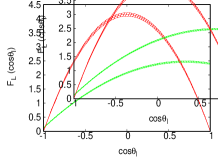
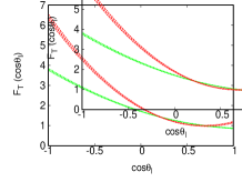
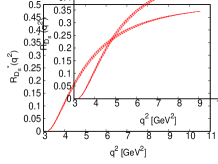
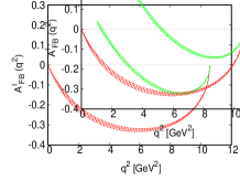
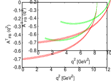
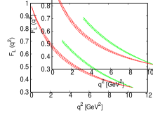
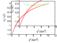
Figure 1: $q^{2}$ and $\cos\theta_{l}$ dependence of $B_{s}\to D_{s}^{*}\,(\to D_{s}\gamma,D_{s}\pi)\,l\nu$ decay observables in the SM for the $e$ (red) and the $\tau$ (green) mode.

In Fig 2, we display the $q^{2}$ and $\cos\theta_{D_{s}}$ dependence of several observables that are different for $B_{s}\to D_{s}^{*}(\to D_{s}\pi)\,l\,\nu$ and $B_{s}\to D_{s}^{*}(\to D_{s}\gamma)\,l\,\nu$ decay modes. Here the red color represents the $e$ mode and green color represents the $\tau$ mode, respectively. Our observations are as follows.

• DBR : In case of $B_{s}\to D_{s}^{*}(\to D_{s}\gamma)\,l\,\nu$ decay mode, the maximum value of ${\rm DBR}=(0.567\,\pm\,0.037)\times 10^{-2}$ is observed at $q^{2}\approx 6.04\,\rm GeV^{2}\rm$ for the $e$ mode, whereas, the maximum value of ${\rm DBR}=(0.241\pm 0.015)\times 10^{-2}$ is observed at $q^{2}\approx 8.28\,\rm GeV^{2}\rm$ for the $\tau$ mode. Similarly, for $B_{s}\to D_{s}^{*}(\to D_{s}\pi)\,l\,\nu$, the $DBR$ peak of $(0.351\pm 0.023)\times 10^{-3}$ is observed at $q^{2}\approx 6.15\rm\,GeV^{2}\rm$ for e mode and maximum ${\rm DBR}=(0.150\pm 0.010)\times 10^{-3}$ is observed at $q^{2}\approx 8.07\rm\,GeV^{2}\rm$ for the $\tau$ mode.

• $A_{3}$, $A_{4}$, $A_{5}$: The angular observables $A_{i}$s obey a strict relation $A_{i}^{\pi}=-2\,A_{i}^{\gamma}$ at all values of $q^{2}$ for the $D_{s}\pi$ and $D_{s}\gamma$ mode.

• $A_{6s}$ : For the $D_{s}\gamma$ channel, $A_{6s}$ is observed to be zero for the $e$ mode, whereas, it is minimum at low $q^{2}$ and maximum at high $q^{2}$ for the $\tau$ mode. It should also be mentioned that value of $A_{6s}$ is negative for the whole $q^{2}$ range. For the $D_{s}\pi$ channel, the maximum of $A_{6s}$ is observed at $q^{2}\approx 5.98\,\rm GeV^{2}$ for the $e$ mode and it is observed at $q^{2}\approx 7.28\,\rm GeV^{2}$ for the $\tau$ mode.

• $F_{L}^{D_{s}^{*}}(\cos{\theta_{D_{s}}})$: The behviour of $F_{L}^{D_{s}^{*}}$ is symmetric about $\cos{\theta_{D_{s}}}$. The maximum value of $F_{L}^{D_{s}^{*}}$ is obtained at $\cos\theta_{D_{s}}=\,0$ for both $e$ and the $\tau$ mode in the $D_{s}\gamma$ mode, whereas, in $D_{s}\pi$ mode, we observe a minimum at $\cos\theta_{D_{s}}=\,0$.

• $F_{T}^{D_{s}^{*}}(\cos{\theta_{D_{s}}})$ : $F_{T}^{D_{s}^{*}}$ is symmetric in $\cos\theta_{D_{s}}$ for both $D_{s}\gamma$ and $D_{s}\pi$ mode. $F_{T}^{D_{s}^{*}}$ is minimum at $\cos\theta_{D_{s}}=0$, whereas, it is found to be maximum at $\cos\theta_{D_{s}}=\pm 1$ for the $D_{s}\gamma$ mode. For the $D_{s}\pi$ mode, the maximum, however, occurs at $\cos\theta_{D_{s}}=0$ and it goes to zero at $\cos\theta_{D_{s}}=\pm 1$.

• $A_{FB}^{l}(\cos\theta_{D_{s}})$ : $A_{FB}^{l}$ is symmetric in $\cos\theta_{D_{s}}$ for both $D_{s}\gamma$ and $D_{s}\pi$ modes. For $D_{s}\gamma$ mode, $A_{FB}^{l}$ is minimum at $\cos\theta=\pm 1$, whereas, it is maximum at $\cos\theta=0$ for both $e$ and the $\tau$ mode. However, for $D_{s}\pi$ mode, it is completely opposite. $A_{FB}^{l}$ is maximum at $\cos\theta=\pm 1$ and minimum at $\cos\theta=0$ for both $e$ and the $\tau$ cases. It should also be mentioned that, a zero crossing in $A_{FB}^{\tau}(\cos\theta_{D_{s}})$ is observed at $\cos\theta_{D_{s}}=\pm 0.456\pm 0.018$ for the $D_{s}\gamma$ mode, whereas, the zero crossing point is observed at $\cos\theta_{D_{s}}=\pm 0.626\pm 0.007$ for the $D_{s}\pi$ mode.

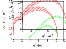
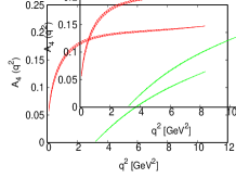
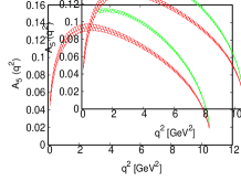
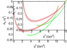
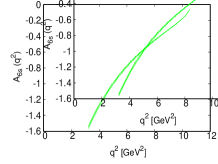
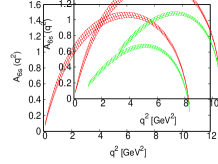
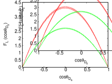
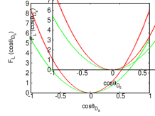
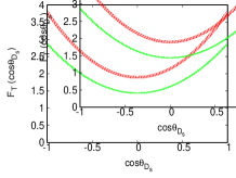
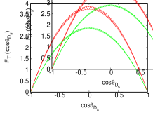
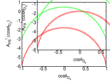
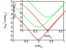
Figure 2: $q^{2}$ and $\cos\theta_{D_{s}}$ dependence of $B_{s}\to D_{s}^{*}\,(\to D_{s}\gamma,D_{s}\pi)\,l\nu$ decay observables in the SM for the $e$ (red) and the $\tau$ (green) mode.

III.3 New physics analysis

We now proceed to discuss the NP effects on various physical observables in the angular distribution of $B_{s}\to D_{s}^{*}(\to D_{s}\gamma)\,\tau\,\nu$ and $B_{s}\to D_{s}^{*}(\to D_{s}\pi)\,\tau\,\nu$ decays in a model independent framework. We have taken three possible NP scenarios. The best fit values of the NP couplings under each scenarios, taken from recent global fit analysis Blanke:2018yud ; Blanke:2019qrx ; Becirevic:2019tpx , are reported in Table 4.

New physics scenarios
Scenerio - I Blanke:2018yud ; Blanke:2019qrx	Scenerio - II Blanke:2018yud ; Blanke:2019qrx	Scenerio - III Becirevic:2019tpx
$g_{V_{L}}=0.07$	$(g_{V_{L}},\,g_{S_{L}}=-4\,g_{T_{L}})=(0.10,-0.04)$	$g_{V_{L}}=0.07-i0.16$
$g_{S_{R}}=0.09$	$(g_{S_{R}},\,g_{S_{L}})=(0.21,-0.15)(SetA)$ or	$g_{V_{R}}=-0.01-i0.39$
$g_{S_{L}}=0.07$	$(g_{S_{R}},\,g_{S_{L}})=(-0.26,-0.61)(SetB)$	$g_{S_{L}}=0.29-i0.67$
$g_{S_{L}}=4\,g_{T_{L}}=-0.03$	$(g_{V_{L}},\,g_{S_{R}})=(0.08,-0.01)$	$g_{S_{R}}=0.19+i0.08$
	$(g_{S_{L}}=4\,g_{T_{L}})=(-0.06+i0.31)$	$g_{T_{L}}=0.11-i0.18$

Table 4: Best fit value of NP couplings.

III.3.1 Scenerio - I

In scenerio - I, we choose four different 1D NP hypothesis and the corresponding best fit values of Ref Blanke:2018yud ; Blanke:2019qrx obtained at scale $\mu=1\,{\rm TeV}$ are reported in Table 4. For our analysis, we run these NP couplings down to the renormalization scale $\mu=m_{b}$ Blanke:2018yud ; Blanke:2019qrx . The effect of these NP couplings on several physical observables pertaining to $B_{s}\to D_{s}^{*}(\to D_{s}\gamma)\,\tau\,\nu$ and $B_{s}\to D_{s}^{*}(\to D_{s}\pi)\,\tau\,\nu$ decay modes are reported in Table 5.

It is clear from from Table 5 that in the presence of $g_{V_{L}}$ NP coupling, the branching ratio gets considerable deviations from the SM predication. However, no deviation from the SM prediction is observed for observables that are in the form of ratios. The NP dependency cancels in these ratios. In the presence of $g_{S_{L}}$ and $g_{S_{R}}$ NP couplings, $A_{FB}^{\tau}$ is found to be at more than $4\sigma$ away from the SM prediction for both $D_{s}\gamma$ and $D_{s}\pi$ mode. Similarly, a deviation of around $3.4\sigma$, $4.71\sigma$ and $1\sigma$ is observed for $F_{L}^{D_{s}^{*}}$ in the presence of $g_{S_{L}}$, $g_{S_{R}}$ and $g_{S_{L}}=4\,g_{T_{L}}$ NP couplings. Moreover, the deviation from the SM expectation observed in case of $R_{D_{s}^{*}}$ is at the level of $2.05\sigma$ and $3.96$ significance in the presence of $g_{S_{R}}$ and $g_{S_{L}}=4\,g_{T_{L}}$ NP couplings respectively, whereas, it is at the level of $15\sigma$ significance for $g_{V_{L}}$ NP coupling. The observables $A_{3}$ and $A_{FB}^{T}$ show slight deviation from the SM in the presence of $g_{S_{L}}=4\,g_{T_{L}}$ NP coupling. As expected, $A_{7}$, $A_{8}$ and $A_{9}$ are all zero and hence we don’t report them in Table. 5.

	$g_{V_{L}}$		$g_{S_{L}}$		$g_{S_{R}}$		$g_{S_{L}}=4\,g_{T_{L}}$
	$D_{s}\gamma$	$D_{s}\pi$	$D_{s}\gamma$	$D_{s}\pi$	$D_{s}\gamma$	$D_{s}\pi$	$D_{s}\gamma$	$D_{s}\pi$
$BR\times 10^{-2}$	$1.3686\pm 0.0426$	$0.0849\pm 0.0026$	$1.1798\pm 0.0367$	$0.0732\pm 0.0023$	$1.2174\pm 0.0379$	$0.0755\pm 0.0024$	$1.2382\pm 0.0385$	$0.0768\,\pm\,0.0024$
$A_{3}$	$0.0081\pm 0.0001$	$-0.0162\pm 0.0001$	$0.0082\,\pm\,0.0001$	$-0.0164\pm 0.0001$	$0.0080\,\pm\,0.0001$	$-0.0159\,\pm\,0.0001$	$0.0078\,\pm\,0.0001$	$-0.0156\pm\,0.0001$
$A_{4}$	$-0.0442\pm 0.0001$	$0.0883\pm 0.0001$	$-0.0448\pm 0.0001$	$0.0895\pm 0.0001$	$-0.0434\pm 0.0001$	$0.0867\,\pm\,0.0001$	$-0.0426\,\pm\,0.0001$	$0.0852\pm 0.0001$
$A_{5}$	$0.1133\pm 0.0005$	$-0.2265\pm 0.0010$	$0.1104\pm 0.0005$	$-0.2208\pm 0.0010$	$0.1166\pm 0.0005$	$-0.2333\,\pm\,0.0010$	$0.1119\pm 0.0005$	$-0.2238\pm 0.0010$
$A_{6s}$	$-0.5509\pm 0.0026$	$0.9539\,\pm\,0.0077$	$-0.5076\pm 0.0025$	$0.9665\pm 0.0078$	$-0.6033\pm 0.0028$	$0.9366\,\pm\,0.0076$	$-0.5673\pm 0.0027$	$0.9098\pm 0.0075$
$R_{D_{s}^{*}}$	$0.2782\pm 0.0018$		$0.2398\pm 0.0015$		$0.2475\pm 0.0016$		$0.2517\pm 0.0016$
$A_{FB}^{\tau}$	$-0.0896\pm 0.0020$		$-0.1020\pm 0.0020$		$-0.0741\pm 0.0021$		$-0.0761\,\pm\,0.0020$
$A_{FB}^{T}$	$-0.3842\pm 0.0026$		$-0.3842\pm 0.0026$		$-0.3842\pm 0.0026$		$-0.3677\,\pm\,0.0025$
$F_{L}$	$0.4482\pm 0.0015$		$0.4409\pm 0.0015$		$0.4582\pm 0.0015$		$0.4501\,\pm\,0.0015$
$C_{F}^{l}$	$-0.0550\pm 0.0014$		$-0.0557\pm 0.0014$		$-0.0540\pm 0.0014$		$-0.0531\,\pm\,0.0013$

Table 5: Prediction of $B_{s}\to D_{s}^{*}(\to D_{s}\gamma,D_{s}\pi)\,\tau\,\nu$ decay observables in Scenerio - I.

In Fig 3 we display the $q^{2}$ and $\cos\theta_{l}$ dependence of several physical observables that exhibit same behaviour for the $D_{s}\gamma$ and $D_{s}\pi$ modes. The contribution coming from $g_{V_{L}},\,g_{S_{L}},\,g_{S_{R}},\,g_{S_{L}}=4\,g_{T_{L}}$ NP couplings are represented by blue, black, violet and orange lines, respectively. Our observations are as follows.

• In case of $F_{L}(\cos\theta_{l})$, a slight deviation from SM expectation is observed at $\cos\theta_{l}\geq 0.5$ with $g_{S_{L}}$ and $g_{S_{R}}$ NP couplings and they are distinguishable from the SM prediction at slightly more than $1\sigma$ significance. However, for $F_{T}(\cos\theta_{l})$, no such deviation is observed and they all lie within the SM error band.

• In case of $R_{D_{s}^{*}}(q^{2})$, maximum deviation is observed in case of $g_{V_{L}}$ NP coupling and it is clearly distinguishable from the SM prediction at more than $3\sigma$ significance at high $q^{2}$ value.

• The zero crossing in $A_{FB}^{\tau}(q^{2})$ is shifted to lower value of $q^{2}$ than in the SM with $g_{S_{L}}$ NP coupling, whereas, it is found to be shifted to higher value of $q^{2}$ with $g_{S_{R}}$ and $g_{S_{L}}=4\,g_{T_{L}}$ NP couplings. The zero crossings in $A_{FB}^{\tau}$ at $q^{2}=5.06\,{\rm GeV^{2}}$, $q^{2}=5.48\,{\rm GeV^{2}}$ and $q^{2}=5.43\,{\rm GeV^{2}}$ in the presence of $g_{S_{L}}$, $g_{S_{R}}$ and $g_{S_{L}}=4\,g_{T_{L}}$ NP couplings are clearly distinguishable from the SM prediction of $q^{2}=5.25\pm 0.12\,{\rm GeV^{2}}$ at the level of $1.9\sigma$ and $2.3\sigma$ and $1.7\sigma$ significance.

• At low $q^{2}$ range, $A_{FB}^{T}(q^{2})$ is deviates from the SM predication in the presence of $g_{S_{L}}=4\,g_{T_{L}}$ NP coupling. In case of $F_{L}^{D_{s}^{*}}(q^{2})$ and $C_{F}^{\tau}(q^{2})$ observables, no significant deviation is observed and they all lie within the SM error band.

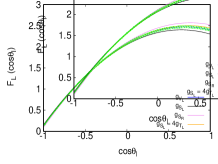
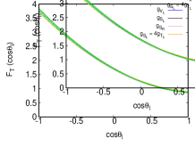
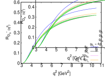
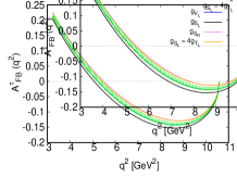
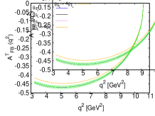
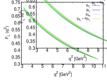
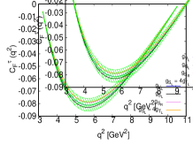
Figure 3: The $q^{2}$ and $\cos\theta_{l}$ dependence of $B_{s}\to D_{s}^{*}(\to D_{s}\gamma,D_{s}\pi)\tau\nu$ decay observables in the SM and in the presence of the NP couplings of scenario - I. The SM central line and the corresponding error band are shown with green color. The blue, black, violet and orange lines represent the effect of $g_{V_{L}},\,g_{S_{L}},\,g_{S_{R}},\,g_{S_{L}}=4\,g_{T_{L}}$ NP couplings, respectively.

In Fig 4 we display the $q^{2}$ and $\cos\theta_{D_{s}}$ dependence of several physical observables that exhibits different behaviour for the $D_{s}\gamma$ and $D_{s}\pi$ decay modes. Our observations are as follows.

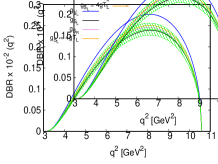
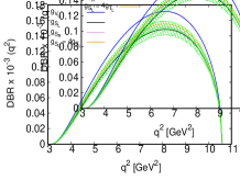
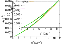
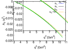
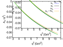
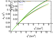
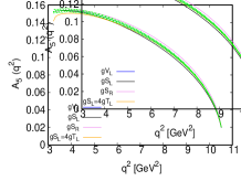
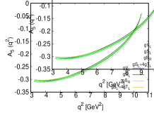
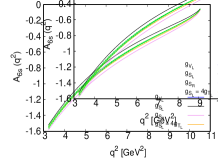
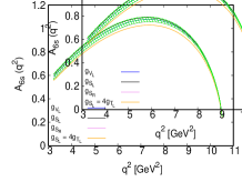
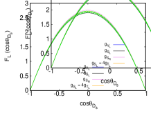
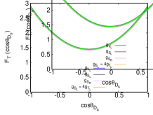
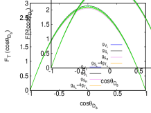
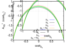
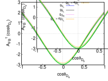
Figure 4: The $q^{2}$ and $\cos\theta_{D_{s}}$ dependence of various physical observable of $B_{s}\to D_{s}^{*}(\to D_{s}\gamma,D_{s}\pi)\tau\nu$ in the SM and in the presence of the NP couplings of scenario - I. The SM central line and the corresponding error band are shown with green color. The blue, black, violet and orange colors represents the effect of NP coupling $g_{V_{L}},\,\ g_{S_{L}},\,\ g_{S_{R}},\,\ g_{S_{L}}=4\,g_{T_{L}}$ respectively.

• In case of differential branching ratio $DBR\,(q^{2})$, the deviation from the SM prediction is more pronounced with $g_{V_{L}}$ NP coupling and the peak of the distribution is clearly distinguishable from the SM prediction at the level of $2\sigma$ significance. No such significant deviation is observed with the rest of the NP couplings and they all lie within the SM error band.

• The angular observable $A_{3}$, $A_{4}$ and $A_{5}$ are slightly deviated from the SM in the presence of $g_{S_{L}}=4g_{T_{L}}$ NP coupling. Similarly in case of $A_{6s}$, a slight deviation is observed with $g_{S_{L}}$, $g_{S_{R}}$ and $g_{S_{L}}=4g_{T_{L}}$ NP coupling for the $D_{s}\gamma$ mode, whereas, $A_{6s}$ shows slight deviation in the presence of $g_{S_{L}}=4g_{T_{L}}$ for the $D_{s}\pi$ mode.

• The observables $F_{L}(\cos{\theta_{D_{s}}})$ and $F_{T}(\cos{\theta_{D_{s}}})$ do not show any significant deviation from the SM prediction in the presence of the NP couplings of scenario - I.

• The deviation from the SM prediction observed in case of $A_{FB}^{\tau}\,(\cos\theta_{D_{s}})$ is more pronounced with $g_{S_{L}}$, $g_{S_{R}}$ and $g_{S_{L}}=4\,g_{T_{L}}$ NP couplings for the $D_{s}\gamma$ mode. The zero crossing in $A_{FB}^{\tau}\,(\cos\theta_{D_{s}})$ is shifted to $\cos\theta_{D_{s}}=0.412$, $0.500$ and $0.497$ in the presence of $g_{S_{L}}$, $g_{S_{R}}$ and $g_{S_{L}}=4\,g_{T_{L}}$ NP couplings and they are clearly distinguishable from the SM zero crossing of $\cos\theta_{D_{s}}=\pm 0.456\pm 0.018$ at the level of more than $2\sigma$ significance. Similarly for the $D_{s}\pi$ mode, $A_{FB}^{\tau}\,(\cos\theta_{D_{s}})$ shows slight deviation in the presence of $g_{S_{L}}$, $g_{S_{R}}$ and $g_{S_{L}}=4\,g_{T_{L}}$ NP couplings. The zero crossings in $A_{FB}^{\tau}\,(\cos\theta_{D_{s}})$ observed at $\cos\theta_{D_{s}}=\pm 0.642$, $\pm 0.610$ and $\pm 0.613$ in the presence of $g_{S_{L}}$, $g_{S_{R}}$ and $g_{S_{L}}=4\,g_{T_{L}}$ NP couplings are distinguishable from the SM zero crossing of $\cos\theta_{D_{s}}=\pm 0.626\pm 0.007$ at the level of $1-2\sigma$ significance.

III.3.2 (Scenerio - II)

In scenerio-II, we choose four 2D NP hypothesis such as ($g_{V_{L}}$, $g_{S_{L}}\,=\,-4g_{T_{L}}$), ($g_{S_{R}}$, $g_{S_{L}}$)(Set A or Set B), ($g_{V_{L}}$, $g_{S_{R}}$) and ($g_{S_{L}}\,=\,4g_{T_{L}}$). The best fit values of these NP couplings at $\mu=1\rm TeV$ scale obtained from Ref. Blanke:2018yud ; Blanke:2019qrx are mentioned in the Table 4. In our analysis, we run them down to the renormalization scale of $\mu=m_{b}$. In Table 6, we report the central values and the corresponding $1\sigma$ range of several physical observables for both $B_{s}\to(D_{s}\gamma)\,\tau\,\nu$ and $B_{s}\to(D_{s}\pi)\,\tau\,\nu$ decays in the presence of each $2D$ NP couplings.

The deviation from the SM prediction observed for $BR$ is more pronounced in the presence of $(g_{V_{L}}$, $g_{S_{L}}\,=\,-4g_{T_{L}})$ NP coupling and it is clearly distinguishable from the SM prediction at more than $3\sigma$ significance. Similarly, a deviation of around $2-3\sigma$ is observed with $(g_{S_{R}},\,g_{S_{L}})$ (setA or Set B) and $(g_{V_{L}},\,g_{S_{R}})$ NP couplings. Significant deviation from the SM prediction is observed for $R_{D_{s}^{*}}$ with $(g_{V_{L}}$, $g_{S_{L}}\,=\,-4g_{T_{L}})$, $(g_{V_{L}},\,g_{S_{R}})$ and $(g_{S_{R}},\,g_{S_{L}})$ (set A or Set B) NP couplings. In case of $F_{L}^{D_{s}^{*}}$, the deviation is more pronounced with $(g_{S_{R}},\,g_{S_{L}})$ (set A or Set B) NP couplings. The angular observable $A_{7}$ is found to be non zero in the presence of $(g_{S_{L}}=4g_{T_{L}})$ complex NP couplings for both $D_{s}\gamma$ and $D_{s}\pi$ modes. The angular observables $A_{8}$ and $A_{9}$ are absent in this scenario-II and hence we do not report them in Table- 6.

	( $g_{V_{L}}$, $g_{S_{L}}\,=\,-4g_{T_{L}}$)		($g_{S_{R}}$, $g_{S_{L}}$)(Set A)		($g_{S_{R}}$, $g_{S_{L}}$)(Set B)		( $g_{V_{L}}$, $g_{S_{R}}$)		$g_{S_{L}}=4g_{T_{L}}$
	$D_{s}\gamma$	$D_{s}\pi$	$D_{s}\gamma$	$D_{s}\pi$	$D_{s}\gamma$	$D_{s}\pi$	$D_{s}\gamma$	$D_{s}\pi$	$D_{s}\gamma$	$D_{s}\pi$
$BR\times 10^{-2}$	$1.4049\pm 0.0437$	$0.0872\,\pm\,0.0027$	$1.2984\pm 0.0404$	$0.0805\,\pm\,0.0025$	$1.2963\pm 0.0404$	$0.0804\pm 0.0025$	$1.3918\pm 0.0433$	$0.0863\,\pm\,0.0027$	$1.3696\pm 0.0426$	$0.0850\pm 0.0026$
$A_{3}$	$0.0083\,\pm\,0.0001$	$-0.0167\,\pm\,0.0001$	$0.0075\,\pm\,0.0001$	$-0.0149\,\pm\,0.0001$	$0.0075\,\pm\,0.0001$	$-0.0150\pm 0.0001$	$0.0081\,\pm\,0.0001$	$-0.0162\,\pm\,0.0001$	$0.0066\pm 0.0001$	$-0.0132\pm 0.0001$
$A_{4}$	$-0.0454\,\pm\,0.0001$	$0.0909\,\pm\,0.0002$	$-0.0407\,\pm\,0.0001$	$0.0813\,\pm\,0.0002$	$-0.0407\,\pm\,0.0001$	$0.0815\,\pm\,0.0002$	$-0.0443\,\pm\,0.0001$	$0.0885\,\pm\,0.0001$	$-0.0359\pm 0.0001$	$0.0719\pm 0.0001$
$A_{5}$	$0.1178\,\pm\,0.0005$	$-0.2356\,\pm\,0.0010$	$0.1247\,\pm\,0.0004$	$-0.2493\,\pm\,0.0009$	$0.1245\,\pm\,0.0004$	$-0.2490\,\pm\,0.0009$	$0.1129\,\pm\,0.0005$	$-0.2258\,\pm\,0.0010$	$0.1084\pm 0.0004$	$-0.2168\pm 0.0008$
$A_{6s}$	$-0.5736\,\pm\,0.0028$	$0.9950\,\pm\,0.0079$	$-0.7422\,\pm\,0.0030$	$0.8782\,\pm\,0.0072$	$-0.7394\,\pm\,0.0030$	$0.8796\pm 0.0072$	$-0.5453\,\pm\,0.0026$	$0.9556\,\pm\,0.0078$	$-0.6032\pm 0.0027$	$0.7508\pm 0.0061$
$A_{7}$	0.0000		0.0000		0.0000		0.0000		$0.0086\pm 0.0001$	$0.0172\pm 0.0001$
$R_{D_{s}^{*}}$	$0.2856\,\pm\,0.0018$		$0.2639\,\pm\,0.0018$		$0.2635\,\pm\,0.0018$		$0.2829\pm 0.0018$		$0.2784\pm 0.0018$
$A_{FB}^{\tau}$	$-0.0936\pm 0.0021$		$-0.0302\pm 0.0021$		$-0.0311\pm 0.0021$		$-0.0912\pm 0.0020$		$-0.0328\pm 0.0017$
$A_{FB}^{T}$	$-0.4047\,\pm\,0.0026$		$-0.3842\,\pm\,0.0026$		$-0.3842\,\pm\,0.0026$		$-0.3842\,\pm\,0.0026$		$-0.3000\,\pm\,0.0017$
$F_{L}$	$0.4537\,\pm\,0.0015$		$0.4920\,\pm\,0.0015$		$0.4912\,\pm\,0.0015$		$0.4472\,\pm\,0.0015$		0.4438 $\pm$ 0.0015
$C_{F}^{l}$	$-0.0567\,\pm\,0.0014$		$-0.0506\,\pm\,0.0013$		$-0.0507\,\pm\,0.0013$		$-0.0551\,\pm\,0.0014$		$-0.0559\pm 0.0011$

Table 6: Prediction of $B_{s}\to D_{s}^{*}(\to D_{s}\gamma,D_{s}\pi)\,\tau\,\nu$ decay observables in Scenerio - II.

We display the $q^{2}$ and $\cos\theta_{l}$ dependence of several physical observables that show same behaviour for the $D_{s}\gamma$ and $D_{s}\pi$ decay modes in Fig 5. The blue, black, yellow, violet and red lines represent the contribution coming from $(g_{V_{L}}$, $g_{S_{L}}\,=\,-4g_{T_{L}})$, $(g_{S_{R}}$, $g_{S_{L}})$ (Set A), $(g_{S_{R}}$, $g_{S_{L}})$ (Set B), $(g_{V_{L}}$, $g_{S_{R}})$ and $(g_{S_{L}}\,=\,4g_{T_{L}})$ NP couplings, respectively. Our observations are as follows.

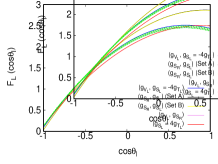
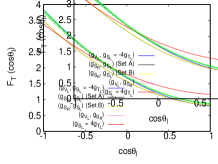
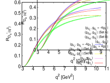
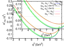
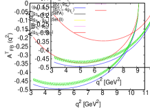
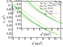
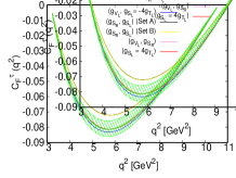
Figure 5: The $q^{2}$ and $\cos\theta_{l}$ dependence of various physical observable of $B_{s}\to D_{s}^{*}(\to D_{s}\gamma,D_{s}\pi)\tau\nu$ in the SM and in the presence of the NP couplings of scenario - II. The SM central line and the corresponding error band are shown with green color. The blue, black, yellow, violet and red color colors represents the effect of NP coupling ($g_{V_{L}}$, $g_{S_{L}}\,=\,-4g_{T_{L}}$), ($g_{S_{R}}$, $g_{S_{L}}$)(Set A), ($g_{S_{R}}$, $g_{S_{L}}$)(Set B), ($g_{V_{L}}$, $g_{S_{R}}$) and $g_{S_{L}}\,=\,4g_{T_{L}}$ respectively.

• Although a slight deviation from the SM prediction is observed for $F_{L}(\cos\theta_{l})$ with $g_{S_{L}}\,=\,4g_{T_{L}}$ NP coupling, the deviation, however, is quite significant in the presence of $(g_{S_{R}}$, $g_{S_{L}})$ (Set A or Set B) NP couplings. Similarly, $F_{T}(\cos\theta_{l})$ is observed to be deviated from the corresponding SM value in the presence of $(g_{S_{R}}$, $g_{S_{L}})$ (Set A or Set B) and $(g_{S_{L}}\,=\,4g_{T_{L}})$ NP couplings.

• Although the deviation from the SM prediction for $R_{D_{s}^{*}}(q^{2})$ is quite significant for all the $2D$ NP couplings, it is more pronounced in case of $(g_{V_{L}}$, $g_{S_{L}}\,=\,-4g_{T_{L}})$, $(g_{V_{L}}$, $g_{S_{R}})$ and $(g_{S_{L}}=4g_{T_{L}})$ NP couplings and they are clearly distinguishable from the SM prediction at more than $10\sigma$ significance.

• The zero crossing in $A_{FB}^{\tau}(q^{2})$ is shifted to higher value of $q^{2}$ than in the SM in the presence of $(g_{S_{R}}$, $g_{S_{L}})$  (Set A or Set B) and $(g_{S_{L}}=4g_{T_{L}})$ NP couplings. The zero crossings of $A_{FB}^{\tau}(q^{2})$ at $q^{2}=6.28{\rm GeV^{2}}$ and $q^{2}=6.16{\rm GeV^{2}}$ in the presence of these NP couplings are clearly distinguishable from the SM prediction of $q^{2}=5.25\pm 0.10{\rm GeV^{2}}$ at more than $8\sigma$ significance. Similarly, for $A_{FB}^{T}(q^{2})$, a significant deviation of more than $10\sigma$ is observed at low $q^{2}$ in the presence of $g_{S_{L}}=4g_{T_{L}}$ NP coupling.

• In case of $F_{L}(q^{2})$, although a slight deviation is observed with $(g_{S_{L}}\,=\,4g_{T_{L}})$ NP coupling, the deviation, however, is more pronounced in the presence of $(g_{S_{R}}$, $g_{S_{L}})$ (Set A or Set B) NP couplings. Similarly for $C_{F}^{\tau}(q^{2})$, maximum deviation from the SM prediction is observed with $(g_{S_{R}}$, $g_{S_{L}})$ (Set A or Set B) NP couplings.

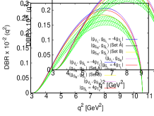
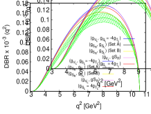
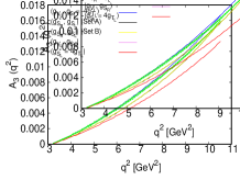
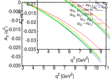
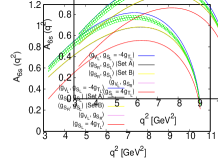
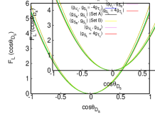
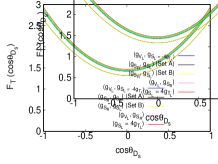
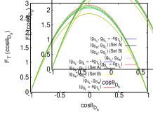
Figure 6: The $q^{2}$ and $\cos\theta_{D_{s}}$ dependence of various physical observable of $B_{s}\to D_{s}^{*}(\to D_{s}\gamma,D_{s}\pi)\tau\nu$ in the SM and in the presence of the NP couplings of scenario - II. The SM central line and the corresponding error band are shown with green color. The blue, black, yellow, violet and red color colors represents the effect of NP coupling ($g_{V_{L}}$, $g_{S_{L}}\,=\,-4g_{T_{L}}$), ($g_{S_{R}}$, $g_{S_{L}}$)(Set A), ($g_{S_{R}}$, $g_{S_{L}}$)(Set B), ($g_{V_{L}}$, $g_{S_{R}}$) and $g_{S_{L}}\,=\,4g_{T_{L}}$ respectively.

The $q^{2}$ and $\cos\theta_{D_{s}}$ dependent observables which exhibit different behaviour for $D_{s}\pi$ and $D_{s}\gamma$ modes are displayed in Fig 6. The left panel figures correspond to the $D_{s}\gamma$ mode and right panel figures correspond to the $D_{s}\pi$ mode, respectively. Our observations are as follows.

• In case of $DBR(q^{2})$, although there is deviation from the SM prediction with all NP couplings, the deviation, however, is more pronounced once the $(g_{V_{L}}$, $g_{S_{L}}\,=\,-4g_{T_{L}})$ NP coupling is switched on and it is clearly distinguishable from the SM prediction at more than $3\sigma$ significance level.

• For the $A_{3}$, $A_{4}$ and $A_{5}$ observables, the maximum deviation is observed in case of $(g_{S_{L}}\,=\,4g_{T_{L}})$ NP couplings for both $D_{s}\pi$ and $D_{s}\gamma$ modes. For $A_{6s}$, the maximum deviation is observed with $(g_{S_{R}}$, $g_{S_{L}})$ (Set A or Set B) for the $D_{s}\gamma$ mode, whereas, for the $D_{s}\pi$ mode, the maximum deviation is observed with $(g_{S_{L}}\,=\,4g_{T_{L}})$ NP coupling.

• For the $D_{s}\gamma$ mode, $F_{L}(\cos{\theta_{D_{s}}})$ deviates significantly from the SM prediction at $\cos\theta_{D_{s}}=0$ in presence of $(g_{S_{R}}$, $g_{S_{L}})$ (Set A or Set B) NP coupling and it is clearly distinguishable from the SM error band, whereas, for the $D_{s}\pi$ mode, $F_{L}(\cos{\theta_{D_{s}}})$ shows a significant deviation at $\cos\theta_{D_{s}}=\pm 1$. In case of $F_{T}(\cos{\theta_{D_{s}}})$, the deviation from the SM prediction is more pronounced with $(g_{S_{R}}$, $g_{S_{L}})$  (Set A or Set B) NP couplings for both $D_{s}\pi$ and $D_{s}\gamma$ modes.

• For $D_{s}\gamma$ and $D_{s}\pi$ mode, $A_{FB}^{\tau}(\cos{\theta_{D_{s}}})$ deviates significantly from the SM prediction in the presence of $(g_{S_{R}}$, $g_{S_{L}})$ (Set A or Set B) and $(g_{S_{L}}\,=\,4g_{T_{L}})$ NP couplings. The zero crossings in $A_{FB}^{\tau}(\cos{\theta_{D_{s}}})$ at $\cos{\theta_{D_{s}}}=\pm 0.601$ and $\cos{\theta_{D_{s}}}=\pm 0.563$ for $D_{s}\gamma$ and $D_{s}\pi$ modes lie $8\sigma$ away from the SM zero crossing point.

• We observe a non-zero $q^{2}$ distribution of $A_{7}(q^{2})$ in the presence of $g_{S_{L}}\,=\,4g_{T_{L}}$ complex NP couplings.

III.3.3 (Scenerio - III)

In this scenario, we select five different complex $1D$ NP couplings. The best fit values each NP couplings at renormalization scale $\mu=m_{b}$ obtained from RefBecirevic:2019tpx are reported in Table 4. In Table 7, we report the impact of each NP couplings on various physical observable in $D_{s}\gamma$ and $D_{s}\pi$ decay modes. We see significant deviation of all the observables with these complex NP couplings. In the presence of $g_{V_{L}}$ and $g_{V_{R}}$ NP couplings, branching ratio deviates from the SM prediction at the level of $3-6\sigma$ significance. $A_{FB}^{\tau}$ deviates more than $9\sigma$ in the presence of $g_{V_{R}}$ and $g_{S_{L}}$ NP couplings and the observable $A_{FB}^{T}$ deviates more than $10\sigma$ from the SM expectation in case of $g_{V_{R}}$ NP coupling. Similarly, the longitudinal polarization fraction of $D_{s}^{*}$, $F_{L}$ is found to deviate from the SM value at more than $10\sigma$ significance in the presence of $g_{T_{L}}$ NP coupling for both the decay modes. In case of $R_{D_{s}^{*}}$, we observe a considerable deviation of around $10\sigma$ in the presence of $g_{V_{L}}$ and $g_{T_{L}}$ NP couplings. Moreover, for $A_{3}\,A_{4},\,{\rm and}\,A_{5}$ the maximum deviation from the SM prediction is observed with $g_{T_{L}}$ NP coupling. For the angular observable $A_{6s}$, the deviation observed is more pronounced in case of $g_{S_{L}}$, $g_{S_{R}}$ and $g_{T_{L}}$ NP couplings in $D_{s}\gamma$ mode, whereas, $g_{V_{L}}$ and $g_{T_{L}}$ show more significant deviation in case of $D_{s}\pi$ mode. A nonzero value of $A_{7}$ is also observed in the presence of $g_{S_{L}}$, $g_{S_{R}}$ and $g_{T_{L}}$ NP couplings. The angular observables $A_{8}$ and $A_{9}$ assume non zero values once $g_{V_{R}}$ NP coupling is switched on It should also be mentioned that the values of $A_{7}$, $A_{8}$ and $A_{9}$ in $D_{s}\pi$ mode is twice as large as the values obtained for the $D_{s}\gamma$ mode.

	$g_{V_{L}}$		$g_{V_{R}}$		$g_{S_{L}}$		$g_{S_{R}}$		$g_{T_{L}}$
	$D_{s}\gamma$	$D_{s}\pi$	$D_{s}\gamma$	$D_{s}\pi$	$D_{s}\gamma$	$D_{s}\pi$	$D_{s}\gamma$	$D_{s}\pi$	$D_{s}\gamma$	$D_{s}\pi$
$BR\times 10^{-2}$	$1.3992\,\pm\,0.0436$	$0.0868\,\pm\,0.0027$	$1.3980\,\pm\,0.0435$	$0.0867\,\pm\,0.0027$	$1.1831\,\pm\,0.0368$	$0.0734\,\pm\,0.0023$	$1.2228\,\pm\,0.0381$	$0.0759\,\pm\,0.0024$	$1.3681\,\pm\,0.0429$	$0.0849\,\pm\,0.0027$
$A_{3}$	$0.0081\,\pm\,0.0001$	$-0.0162\,\pm\,0.0001$	$0.0082\,\pm\,0.0001$	$-0.0163\,\pm\,0.0001$	$0.0082\,\pm\ 0.0001$	$-0.0164\,\pm\,0.0001$	$0.0079\,\pm\,0.0001$	$-0.0159\,\pm\,0.0001$	$-0.0019\,\pm\,0.0001$	$-0.0038\,\pm\,0.0001$
$A_{4}$	$-0.0442\,\pm\,0.0001$	$0.0883\,\pm\,0.0001$	$-0.0443\,\pm\,0.0001$	$0.0886\,\pm\,0.0001$	$-0.0446\,\pm\ 0.0001$	$0.0893\,\pm\,0.0001$	$-0.0432\,\pm\,0.0001$	$0.0864\,\pm\,0.0001$	$-0.0112\,\pm\,0.0001$	$0.0224\,\pm\,0.0002$
$A_{5}$	$0.1133\,\pm\,0.0005$	$-0.2265\,\pm\,0.0010$	$0.0949\,\pm\,0.0004$	$-0.1899\,\pm\,0.0007$	$0.1041\,\pm\ 0.0005$	$-0.2082\,\pm\,0.0010$	$0.1173\,\pm\,0.0005$	$-0.2346\,\pm\,0.0010$	$0.0566\,\pm\,0.0002$	$-0.1132\,\pm\,0.0005$
$A_{6s}$	$-0.5509\,\pm\,0.0026$	$0.9539\,\pm\,0.0077$	$-0.5521\,\pm\,0.0026$	$0.6915\,\pm\,0.0056$	$-0.4374\,\pm\ 0.0022$	$0.9638\,\pm\,0.0078$	$-0.6141\,\pm\,0.0028$	$0.9325\,\pm\,0.0076$	$-0.2392\,\pm\,0.0023$	$0.3422\,\pm\,0.0014$
$A_{7}$	0.0000		$-0.0130\pm 0.0001$	$-0.0260\pm 0.0001$	$-0.0095\pm 0.0001$	$-0.0190\pm 0.0001$	$-0.0011\pm 0.0001$	$-0.0022\pm 0.0001$	$-0.0062\pm 0.00001$	$-0.0124\pm 0.0001$
$A_{8}$	0.0000		$-0.0102\pm 0.0001$	$-0.0205\pm 0.0001$	0.0000		0.0000		0.0000
$A_{9}$	0.0000		$-0.0042\pm 0.0001$	$-0.0083\pm 0.0001$	0.0000		0.0000		0.0000
$R_{D_{s}^{*}}$	$0.2844\,\pm\,0.0018$		$0.2842\,\pm\,0.0018$		$0.2405\pm 0.0015$		$0.2486\,\pm\,0.0016$		$0.2781\,\pm\,0.0022$
$A_{FB}^{\tau}$	$-0.0896\,\pm\,0.0020$		$-0.0310\,\pm\,0.0016$		$-0.1170\,\pm\,0.0020$		$-0.0708\,\pm\,0.0021$		$-0.0229\,\pm\,0.0007$
$A_{FB}^{T}$	$-0.3842\,\pm\,0.0026$		$-0.2790\,\pm\,0.0019$		$-0.3842\,\pm\,0.0026$		$-0.3842\,\pm\,0.0026$		$-0.1124\,\pm\,0.0002$
$F_{L}^{D_{s}^{*}}$	$0.4482\,\pm\,0.0015$		$0.4493\,\pm\,0.0015$		$0.4425\,\pm\ 0.0015$		$0.4606\,\pm\,0.0015$		$0.3237\,\pm\,0.0021$
$C_{F}^{l}$	$-0.0550\,\pm\,0.0014$		$-0.0558\,\pm\,0.0014$		$-0.0555\,\pm\ 0.0014$		$-0.0537\,\pm\,0.0014$		$-0.1316\,\pm\,0.0004$

Table 7: Prediction of $B_{s}\to D_{s}^{*}(\to D_{s}\gamma,D_{s}\pi)\,\tau\,\nu$ decay observables in Scenerio - III.

In Fig 7 we show the $q^{2}$ and $\cos\theta_{l}$ dependence of various physical observables that exhibit same behaviour for the $D_{s}\gamma$ and $D_{s}\pi$ modes. NP contribution coming from $g_{V_{L}}$, $g_{V_{R}}$, $g_{S_{L}}$, $g_{S_{R}}$ and $g_{T_{L}}$ complex NP couplings are shown with blue, red, black, violet and orange colored lines, respectively. Our observations are as follows.

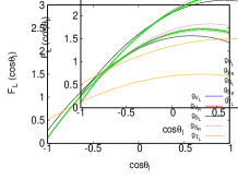
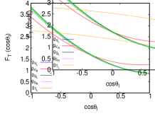
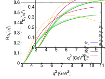
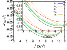
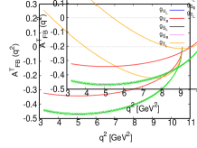
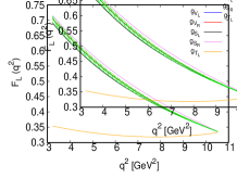
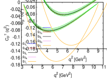
Figure 7: The $q^{2}$ and $\cos\theta_{l}$ dependence of various physical observable of $B_{s}\to D_{s}^{*}(\to D_{s}\gamma,D_{s}\pi)\tau\nu$ in the SM and in the presence of the NP couplings of scenario - III. The SM central line and the corresponding error band are shown with green color. The blue, red, black, violet and orange colors represents the effect of NP coupling $g_{V_{L}}$, $g_{V_{R}}$, $g_{S_{L}}$, $g_{S_{R}}$ and $g_{T_{L}}$ respectively.

• In case of $F_{L}(\cos\theta_{l})$, a significant deviation from the SM prediction is observed due to $g_{T_{L}}$ NP coupling and it is quite distinct from the rest of NP couplings. Similarly, we observe significant deviation in $F_{T}(\cos\theta_{l})$ once $g_{V_{R}}$ and $g_{T_{L}}$ NP couplings are switched on. Again, the behaviour of $F_{T}(\cos\theta_{l})$ is quite distinct with $g_{T_{L}}$ NP coupling.

• In case of $R_{D_{s}^{*}}(q^{2})$, maximum deviation from the SM prediction is observed with $g_{V_{L}}$, $g_{V_{R}}$ and $g_{T_{L}}$ NP couplings and they are clearly distinguishable from the SM prediction. Although the shape of the $q^{2}$ distribution is quite similar for $g_{V_{L}}$ and $g_{V_{R}}$ couplings, it is, however, quite distinct for $g_{T_{L}}$ NP coupling.

• In case of $A_{FB}^{\tau}(q^{2})$, we observe a significant deviation from the SM due to $g_{V_{R}}$, $g_{S_{L}}$, $g_{S_{R}}$ and $g_{T_{L}}$ NP couplings. The zero crossing point is shifted to higher values of $q^{2}$ than in the SM for $g_{V_{R}}$, $g_{S_{R}}$ and $g_{T_{L}}$, whereas, it is shifted to a low value of $q^{2}$ for $g_{S_{L}}$ NP coupling. The observed zero crossings at $q^{2}=6.16\rm GeV^{2}$, $q^{2}=4.82\rm GeV^{2}$, $q^{2}=5.54\rm GeV^{2}$ and $q^{2}=6.49\rm GeV^{2}$ in the presence of $g_{V_{R}}$, $g_{T_{L}}$, $g_{S_{R}}$ and $g_{S_{L}}$ are clearly distinguishable from the SM zero crossing of $q^{2}=5.25\pm 0.10\,{\rm GeV^{2}}$ at the level of $9.1\sigma$, $4.3\sigma$, $2.9\sigma$ and $12\sigma$ significance.

• The observable $A_{FB}^{T}(q^{2})$ shows a significant deviation from SM expectation once $g_{V_{R}}$ and $g_{T_{L}}$ NP couplings are switched on. We also observe a zero crossing in $A_{FB}^{T}(q^{2})$ at $q^{2}=5.44{\rm GeV^{2}}$ with $g_{T_{L}}$ NP coupling. Similarly, a significant deviation from the SM prediction is observed in $C_{F}^{\tau}(q^{2})$ and $F_{L}(q^{2})$ in the presence of $g_{T_{L}}$ NP coupling. The dip in $C_{F}^{\tau}(q^{2})$ is shifted to a higher value of $q^{2}$ than in the SM.

In Fig 8, we display $q^{2}$ and $\cos\theta_{D_{s}}$ dependence of several observable for $D_{s}\gamma$ (left panel) and $D_{s}\pi$ (right panel) modes. Our main observations are as follows.

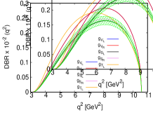
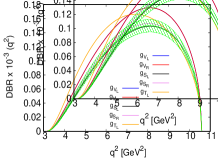
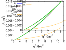
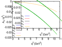
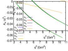
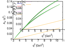
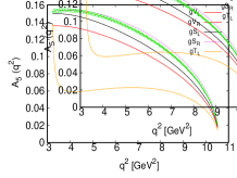
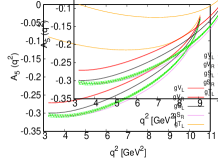
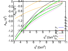
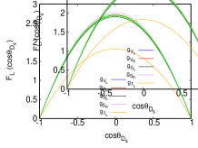
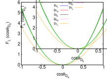
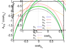
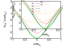
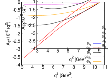
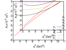
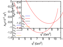
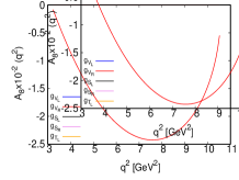
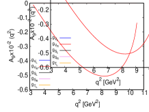
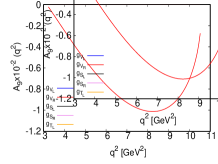
Figure 8: The $q^{2}$ and $\cos\theta_{D_{s}}$ dependence of various physical observable of $B_{s}\to D_{s}^{*}(\to D_{s}\gamma,D_{s}\pi)\tau\nu$ in the SM and in the presence of the NP couplings of scenario - III. The SM central line and the corresponding error band are shown with green color. The blue, red, black, violet and orange colors represents the effect of NP couplings of $g_{V_{L}}$, $g_{V_{R}}$, $g_{S_{L}}$, $g_{S_{R}}$ and $g_{T_{L}}$ respectively.

• In case of $DBR(q^{2})$, we observe significant deviation from the SM prediction with $g_{T_{L}}$, $g_{V_{L}}$ and $g_{V_{R}}$ NP couplings for both $D_{s}\gamma$ and $D_{s}\pi$ modes. The peak of the distribution, however, is shifted to a low value of $q^{2}$ than in the SM with $g_{T_{L}}$ NP coupling.

• The angular observable $A_{3}(q^{2})$ and $A_{4}(q^{2})$ show deviation from the SM in the presence of $g_{T_{L}}$ NP coupling for both $D_{s}\gamma$ and $D_{s}\pi$ modes. Similarly, in case of $A_{5}(q^{2})$, deviation from the SM prediction is observed in the presence of $g_{V_{R}}$, $g_{S_{L}}$ and $g_{T_{L}}$ NP coupling in both the decay modes. The deviation in $A_{5}(q^{2})$, however, is more pronounced with $g_{T_{L}}$ NP coupling.

• Deviation from the SM prediction in $A_{6s}\,(q^{2})$ is observed with $g_{S_{L}}$, $g_{S_{R}}$ and $g_{T_{L}}$ NP couplings for the $D_{s}\gamma$ mode. The deviation is, however, more pronounced in case of $g_{T_{L}}$ NP coupling. Similarly, for $D_{s}\pi$ mode, we see significant deviation in $A_{6s}\,(q^{2})$ in the presence of $g_{V_{R}}$ and $g_{T_{L}}$ NP couplings. We also observe a zero crossing in the $A_{6s}\,(q^{2})$ at $q^{2}=5.46\rm GeV^{2}$ with $g_{T_{L}}$ NP coupling.

• The $A_{7}(q^{2})$ is non-zero with $g_{V_{R}}$, $g_{S_{L}}$, $g_{S_{R}}$ and $g_{T_{L}}$ NP couplings for both $D_{s}\gamma$ and $D_{s}\pi$ decay mode. Similar conclusions can be made for $D_{s}\pi$ mode as well because of the strict $A_{7}^{\pi}=2\,A_{7}^{\gamma}$ relation.

• The angular observables $A_{8}\,(q^{2})$ and $A_{9}\,(q^{2})$ are non-zero only in the presence of $g_{V_{R}}$ NP coupling for both $D_{s}\gamma$ and $D_{s}\pi$ modes. We observe a minimum of $A_{8}(q^{2})$ and $A_{9}(q^{2})$ at $q^{2}=7.5\,{\rm GeV^{2}}$ and $q^{2}=8.28\,{\rm GeV^{2}}$, respectively.

• Although a slight deviation in $F_{L}(\cos\theta_{D_{s}})$ and $F_{T}(\cos\theta_{D_{s}})$ is observed with $g_{S_{R}}$ NP coupling, the deviation, however, is more pronounced with $g_{T_{L}}$ NP coupling for both $D_{s}\gamma$ and $D_{s}\pi$ modes and it is clearly distinguishable from the SM prediction.

• Deviation from the SM prediction in $A_{FB}(\cos\theta_{D_{s}})$ is observed with $g_{V_{R}}$ $g_{S_{L}}$, $g_{S_{R}}$ and $g_{T_{L}}$ NP couplings for both $D_{s}\gamma$ and $D_{s}\pi$ modes. In the $D_{s}\gamma$ mode, we observe that the zero crossing in $A_{FB}(\cos\theta_{D_{s}})$ shifts to lower value of $\cos\theta_{D_{s}}$ than in the SM with $g_{V_{R}}$, $g_{S_{R}}$ and $g_{T_{L}}$ NP couplings, whereas, it shifts to a higher value of $\cos\theta_{D_{s}}$ with $g_{S_{L}}$ NP coupling. The zero crossing points in $A_{FB}(\cos\theta_{D_{s}})$ at $\cos\theta_{D_{s}}=\pm 0.603\,,\pm 0.330\,,\pm 0.512\,{\rm and}\,\pm 0.703$ in the presence of $g_{V_{R}}$, $g_{S_{L}}$, $g_{S_{R}}$ and $g_{T_{L}}$ NP couplings are clearly distinguishable from the SM zero crossing of $\cos\theta_{D_{s}}=\pm 0.454\pm 0.018$ at $8.16\sigma$, $7\sigma$, $3.1\sigma$ and $13\sigma$ significance level, respectively. Similarly, for $D_{s}\pi$ mode, the zero crossing points in $A_{FB}(\cos\theta_{D_{s}})$ at $\cos\theta_{D_{s}}=\pm 0.558\,,\pm 0.663\,,\pm 0.604\,{\rm and}\,\pm 0.500$ in the presence of these NP couplings are clearly distinguishable from the SM zero crossing of $\cos\theta_{D_{s}}=\pm 0.626\pm 0.0075$ at $9\sigma$, $4.9\sigma$, $2.93\sigma$ and $16\sigma$ level of significance, respectively.

IV Conclusions

Motivated by the anomalies present in several $b\to c\,l\,\nu$ quark level transition decays, we perform a detail angular analysis of $B_{s}\to D_{s}^{*}(\to D_{s}\gamma,D_{s}\pi)\,l\,\nu$ decays using the recent lattice QCD form factors. We use the latest global fit results of the possible NP couplings and estimate the effect of each NP couplings on several physical observables pertaining to $D_{s}\pi$ and $D_{s}\gamma$ modes in a model independent effective theory formalism.

We first report the SM results. In the SM, we obtain the branching ratio to be of $\mathcal{O}(10^{-2})$ for $D_{s}\gamma$ channel and $\mathcal{O}(10^{-3})$ for $D_{s}\pi$ channel. The LHCb collaboration reported the first measurement of the branching ratio to be $\mathcal{B}(B_{s}^{0}\,\to\,D_{s}^{*-}\,\mu^{+}\,{\nu}_{\mu})=(5.38\pm 0.25\pm 0.46)\times 10^{-2}$  Aaij:2020hsi ; Aaij:2020xjy and it is in good agreement with our estimated results for the $D_{s}\gamma$ mode. The ratio of branching ratio is found to be $R_{D_{s}^{*}}=0.2430\pm 0.0015$ in the SM.

For our NP analysis we work with three different NP scenarios with the best fit values obtained from various recent global fit results. We assume both real and complex NP couplings in our analysis. We study the underlying observables based on NP contribution coming from single operators ($1D$) as well as from two different operators ($2D$). A brief summary of our results are as follows.

• In scenario - I, the observable $A_{FB}^{\tau}(q^{2})$ is found to be interesting as the zero crossing point observed with $g_{S_{L}}$ and $g_{S_{R}}$ and $g_{S_{L}}=4g_{T_{L}}$ NP couplings stand at $1-2\sigma$ away from the SM zero crossing point. Similarly, the effect of $g_{V_{L}}$ NP coupling is found to be prominent for $DBR(q^{2})$ and $R_{D_{s}^{*}}(q^{2})$.

• In scenerio-II, the deviation from the SM prediction observed for $DBR(q^{2})$ and $R_{D_{s}^{*}}(q^{2})$ is quite significant in the presence of $(g_{V_{L}}$,  $g_{S_{L}}=-4g_{T_{L}})$ and $(g_{V_{L}}$, $g_{S_{R}})$ NP couplings. The zero crossings in $A_{FB}^{\tau}(q^{2})$ with $(g_{S_{R}}$, $g_{S_{L}})$ and $(g_{S_{L}}=4g_{T_{L}})$ NP couplings are clearly distinguishable from the SM zero crossing point at more than $8\sigma$ and $10\sigma$ significance. Similarly, the zero crossing in $A_{FB}^{\tau}(\cos\theta_{D_{s}})$ obtained with $(g_{S_{R}}$, $g_{S_{L}})$ and $(g_{S_{L}}=4g_{T_{L}})$ NP couplings are distinguishable from the SM zero crossing at more than $7\sigma$ for both the $D_{s}\gamma$ mode and $D_{s}\pi$ mode. We find $A_{7}$ to be non-zero only in the presence of $g_{S_{L}}=4g_{T_{L}}$ NP coupling.

• In scenario-III, the zero crossings in $A_{FB}^{\tau}\,(q^{2})$ in the presence of $g_{V_{R}}$, $g_{T_{L}}$, $g_{S_{R}}$ and $g_{S_{L}}$ NP couplings are quite different from the SM zero crossing and they are clearly distinguishable from the SM prediction at the level of $9.1\sigma$, $4.3\sigma$, $2.9\sigma$ and $12\sigma$ significance. We also observe zero crossings in $A_{FB}^{T}\,(q^{2})$ and $A_{6s}(q^{2})$ with $g_{T_{L}}$ NP coupling that are absent in the SM. The angular observable $A_{7}$ is found to be non-zero in the presence of $g_{V_{R}}$, $g_{S_{L}}$, $g_{S_{R}}$ and $g_{T_{L}}$ NP couplings, whereas, $A_{8}$ and $A_{9}$ are found to be non-zero only for $g_{V_{R}}$ NP coupling. Moreover, the zero crossing points in $A_{FB}^{\tau}(\cos\theta_{D_{s}})$ obtained with $g_{V_{R}}$, $g_{S_{L}}$. $g_{S_{R}}$ and $g_{T_{L}}$ NP couplings are clearly distinguishable from the SM zero crossing at more than $8\sigma$, $7\sigma$, $3\sigma$ and $13\sigma$ significance level for the $D_{s}\gamma$ mode and they are distinguishable at more than $9\sigma$, $4\sigma$, $2\sigma$ and $15\sigma$ significance for the $D_{s}\pi$ mode. In general, the deviation from the SM prediction observed with complex tensor NP coupling $g_{T_{L}}$ is more pronounced for all the observables in this scenario.

It should be noted that the angular observables $A_{FB}^{\tau}(q^{2})$ and $A_{FB}^{\tau}(\cos\theta_{D_{s}})$ are quite interesting as they can be used to distinguish between several NP scenarios. Similarly, presence of zero crossings in $A_{FB}^{T}\,(q^{2})$ and $A_{6s}(q^{2})$ would be a clear signal of complex tensor NP coupling. Moreover, the angular observables $A_{7}$, $A_{8}$ and $A_{9}$ will also play an important role in identifying the exact NP Lorentz structures. In conclusion, the results pertaining to $B_{s}\to D_{s}^{*}(\to D_{s}\gamma,D_{s}\pi)\,l\,\nu$ decay observables are very useful to explore ongoing flavor anomalies in $b\to cl\nu$ transitions and, in principle, it can provide us complementary information regarding NP in various $B$ meson decays. At the same time, it can also be useful in determining the value of the CKM matrix element $|V_{cb}|$. Moreover, study of these decay modes both theoretically and experimentally can act as a useful ingredient in maximizing future sensitivity to NP.

References

- (1) J. A. Bailey et al. [MILC Collaboration], “ form factors at nonzero recoil and from 2+1-flavor lattice QCD,” Phys. Rev. D 92, no. 3, 034506 (2015) doi:10.1103/PhysRevD.92.034506 [arXiv:1503.07237 [hep-lat]].
- (2) H. Na et al. [HPQCD Collaboration], ‘ form factors at nonzero recoil and extraction of ,” Phys. Rev. D 92, no. 5, 054510 (2015) Erratum: [Phys. Rev. D 93, no. 11, 119906 (2016)] doi:10.1103/PhysRevD.93.119906, 10.1103/PhysRevD.92.054510 [arXiv:1505.03925 [hep-lat]].
- (3) S. Aoki et al., “Review of lattice results concerning low-energy particle physics,” Eur. Phys. J. C 77, no. 2, 112 (2017) doi:10.1140/epjc/s10052-016-4509-7 [arXiv:1607.00299 [hep-lat]].
- (4) D. Bigi and P. Gambino, “Revisiting ,” Phys. Rev. D 94, no. 9, 094008 (2016) doi:10.1103/PhysRevD.94.094008 [arXiv:1606.08030 [hep-ph]].
- (5) F. U. Bernlochner, Z. Ligeti, M. Papucci and D. J. Robinson, Phys. Rev. D 95, no.11, 115008 (2017) [erratum: Phys. Rev. D 97, no.5, 059902 (2018)] doi:10.1103/PhysRevD.95.115008 [arXiv:1703.05330 [hep-ph]].
- (6) S. Jaiswal, S. Nandi and S. K. Patra, JHEP 12, 060 (2017) doi:10.1007/JHEP12(2017)060 [arXiv:1707.09977 [hep-ph]].
- (7) B. Aubert et al. [BaBar], Phys. Rev. Lett. 104, 011802 (2010) doi:10.1103/PhysRevLett.104.011802 [arXiv:0904.4063 [hep-ex]].
- (8) R. Glattauer et al. [Belle], Phys. Rev. D 93, no.3, 032006 (2016) doi:10.1103/PhysRevD.93.032006 [arXiv:1510.03657 [hep-ex]].
- (9) J. P. Lees et al. [BaBar], “Evidence for an excess of decays,” Phys. Rev. Lett. 109, 101802 (2012) doi:10.1103/PhysRevLett.109.101802 [arXiv:1205.5442 [hep-ex]].
- (10) M. Huschle et al. [Belle], “Measurement of the branching ratio of relative to decays with hadronic tagging at Belle,” Phys. Rev. D 92, no.7, 072014 (2015) doi:10.1103/PhysRevD.92.072014 [arXiv:1507.03233 [hep-ex]].
- (11) A. Abdesselam et al. [Belle Collaboration], “Measurement of and with a semileptonic tagging method,” arXiv:1904.08794 [hep-ex].
- (12) S. Fajfer, J. F. Kamenik and I. Nisandzic, Phys. Rev. D 85, 094025 (2012) doi:10.1103/PhysRevD.85.094025 [arXiv:1203.2654 [hep-ph]].
- (13) D. Bigi, P. Gambino and S. Schacht, JHEP 11, 061 (2017) doi:10.1007/JHEP11(2017)061 [arXiv:1707.09509 [hep-ph]].
- (14) C. Bernard et al., ‘The form factor at zero recoil from three-flavor lattice QCD: A Model independent determination of ,” Phys. Rev. D 79, 014506 (2009) doi:10.1103/PhysRevD.79.014506 [arXiv:0808.2519 [hep-lat]].
- (15) J. A. Bailey et al. [Fermilab Lattice and MILC Collaborations], “Update of from the form factor at zero recoil with three-flavor lattice QCD,” Phys. Rev. D 89, no. 11, 114504 (2014) doi:10.1103/PhysRevD.89.114504 [arXiv:1403.0635 [hep-lat]].
- (16) J. P. Lees et al. [BaBar], Phys. Rev. D 88, no.7, 072012 (2013) doi:10.1103/PhysRevD.88.072012 [arXiv:1303.0571 [hep-ex]].
- (17) S. Hirose et al. [Belle], Phys. Rev. Lett. 118, no.21, 211801 (2017) doi:10.1103/PhysRevLett.118.211801 [arXiv:1612.00529 [hep-ex]].
- (18) S. Hirose et al. [Belle], Phys. Rev. D 97, no.1, 012004 (2018) doi:10.1103/PhysRevD.97.012004 [arXiv:1709.00129 [hep-ex]].
- (19) R. Aaij et al. [LHCb], “Measurement of the ratio of branching fractions ,” Phys. Rev. Lett. 115, no.11, 111803 (2015) [erratum: Phys. Rev. Lett. 115, no.15, 159901 (2015)] doi:10.1103/PhysRevLett.115.111803 [arXiv:1506.08614 [hep-ex]].
- (20) R. Aaij et al. [LHCb], Phys. Rev. D 97, no.7, 072013 (2018) doi:10.1103/PhysRevD.97.072013 [arXiv:1711.02505 [hep-ex]].
- (21) A. Abdesselam et al. [Belle], [arXiv:1904.08794 [hep-ex]].
- (22) M. A. Ivanov, J. G. Korner and P. Santorelli, “The Semileptonic decays of the meson,” Phys. Rev. D 63, 074010 (2001) doi:10.1103/PhysRevD.63.074010 [hep-ph/0007169].
- (23) D. Ebert, R. N. Faustov and V. O. Galkin, “Weak decays of the meson to charmonium and mesons in the relativistic quark model,” Phys. Rev. D 68, 094020 (2003) doi:10.1103/PhysRevD.68.094020 [hep-ph/0306306].
- (24) A. Abd El-Hady, J. H. Munoz and J. P. Vary, “Semileptonic and nonleptonic B(c) decays,” Phys. Rev. D 62, 014019 (2000) doi:10.1103/PhysRevD.62.014019 [hep-ph/9909406].
- (25) W. F. Wang, Y. Y. Fan and Z. J. Xiao, “Semileptonic decays in the perturbative QCD approach,” Chin. Phys. C 37, 093102 (2013) doi:10.1088/1674-1137/37/9/093102 [arXiv:1212.5903 [hep-ph]].
- (26) Y. K. Hsiao and C. Q. Geng, “Branching fractions of decays involving and ,” Chin. Phys. C 41, no. 1, 013101 (2017) doi:10.1088/1674-1137/41/1/013101 [arXiv:1607.02718 [hep-ph]].
- (27) R. Dutta and A. Bhol, “ semileptonic decays within the standard model and beyond,” Phys. Rev. D 96, no. 7, 076001 (2017) doi:10.1103/PhysRevD.96.076001 [arXiv:1701.08598 [hep-ph]].
- (28) R. Dutta, “Exploring , and anomalies,” arXiv:1710.00351 [hep-ph].
- (29) T. D. Cohen, H. Lamm and R. F. Lebed, “Model-independent bounds on ,” JHEP 1809, 168 (2018) doi:10.1007/JHEP09(2018)168 [arXiv:1807.02730 [hep-ph]].
- (30) J. Harrison et al. [HPQCD], Phys. Rev. D 102, no.9, 094518 (2020) doi:10.1103/PhysRevD.102.094518 [arXiv:2007.06957 [hep-lat]].
- (31) S. Hirose et al. [Belle Collaboration], “Measurement of the lepton polarization and in the decay ,” Phys. Rev. Lett. 118, no. 21, 211801 (2017) doi:10.1103/PhysRevLett.118.211801 [arXiv:1612.00529 [hep-ex]].
- (32) S. Hirose et al. [Belle Collaboration], “Measurement of the lepton polarization and in the decay with one-prong hadronic decays at Belle,” Phys. Rev. D 97, no. 1, 012004 (2018) doi:10.1103/PhysRevD.97.012004 [arXiv:1709.00129 [hep-ex]].
- (33) M. Tanaka and R. Watanabe, “New physics in the weak interaction of ,” Phys. Rev. D 87, no. 3, 034028 (2013) doi:10.1103/PhysRevD.87.034028 [arXiv:1212.1878 [hep-ph]].
- (34) A. Abdesselam et al. [Belle Collaboration], “Measurement of the polarization in the decay ,” arXiv:1903.03102 [hep-ex].
- (35) A. K. Alok, D. Kumar, S. Kumbhakar and S. U. Sankar, “ polarization as a probe to discriminate new physics in ,” Phys. Rev. D 95, no. 11, 115038 (2017) doi:10.1103/PhysRevD.95.115038 [arXiv:1606.03164 [hep-ph]].
- (36) Y. Sakaki, M. Tanaka, A. Tayduganov and R. Watanabe, “Probing New Physics with distributions in ,” Phys. Rev. D 91, no. 11, 114028 (2015) doi:10.1103/PhysRevD.91.114028 [arXiv:1412.3761 [hep-ph]].
- (37) P. Biancofiore, P. Colangelo and F. De Fazio, “On the anomalous enhancement observed in decays,” Phys. Rev. D 87, no. 7, 074010 (2013) doi:10.1103/PhysRevD.87.074010 [arXiv:1302.1042 [hep-ph]].
- (38) M. Freytsis, Z. Ligeti and J. T. Ruderman, “Flavor models for ,” Phys. Rev. D 92, no. 5, 054018 (2015) doi:10.1103/PhysRevD.92.054018 [arXiv:1506.08896 [hep-ph]].
- (39) R. Dutta, “ decays within standard model and beyond,” Phys. Rev. D 93, no. 5, 054003 (2016) doi:10.1103/PhysRevD.93.054003 [arXiv:1512.04034 [hep-ph]].
- (40) S. Bhattacharya, S. Nandi and S. K. Patra, “Looking for possible new physics in in light of recent data,” Phys. Rev. D 95, no. 7, 075012 (2017) doi:10.1103/PhysRevD.95.075012 [arXiv:1611.04605 [hep-ph]].
- (41) P. Colangelo and F. De Fazio, “Tension in the inclusive versus exclusive determinations of : a possible role of new physics,” Phys. Rev. D 95, no. 1, 011701 (2017) doi:10.1103/PhysRevD.95.011701 [arXiv:1611.07387 [hep-ph]].
- (42) R. Dutta and A. Bhol, “ leptonic and semileptonic decays within an effective field theory approach,” Phys. Rev. D 96, no. 3, 036012 (2017) doi:10.1103/PhysRevD.96.036012 [arXiv:1611.00231 [hep-ph]].
- (43) A. K. Alok, D. Kumar, J. Kumar, S. Kumbhakar and S. U. Sankar, “New physics solutions for and ,” JHEP 1809, 152 (2018) doi:10.1007/JHEP09(2018)152 [arXiv:1710.04127 [hep-ph]].
- (44) A. Azatov, D. Bardhan, D. Ghosh, F. Sgarlata and E. Venturini, “Anatomy of anomalies,” JHEP 1811, 187 (2018) doi:10.1007/JHEP11(2018)187 [arXiv:1805.03209 [hep-ph]].
- (45) S. Bifani, S. Descotes-Genon, A. Romero Vidal and M. H. Schune, “Review of Lepton Universality tests in decays,” J. Phys. G 46, no. 2, 023001 (2019) doi:10.1088/1361-6471/aaf5de [arXiv:1809.06229 [hep-ex]].
- (46) Z. R. Huang, Y. Li, C. D. Lu, M. A. Paracha and C. Wang, “Footprints of New Physics in Transitions,” Phys. Rev. D 98, no. 9, 095018 (2018) doi:10.1103/PhysRevD.98.095018 [arXiv:1808.03565 [hep-ph]].
- (47) Q. Y. Hu, X. Q. Li and Y. D. Yang, “ transitions in the standard model effective field theory,” Eur. Phys. J. C 79, no. 3, 264 (2019) doi:10.1140/epjc/s10052-019-6766-8 [arXiv:1810.04939 [hep-ph]].
- (48) F. Feruglio, P. Paradisi and O. Sumensari, “Implications of scalar and tensor explanations of ,” JHEP 1811, 191 (2018) doi:10.1007/JHEP11(2018)191 [arXiv:1806.10155 [hep-ph]].
- (49) M. Jung and D. M. Straub, “Constraining new physics in transitions,” JHEP 1901, 009 (2019) doi:10.1007/JHEP01(2019)009 [arXiv:1801.01112 [hep-ph]].
- (50) A. Datta, S. Kamali, S. Meinel and A. Rashed, “Phenomenology of using lattice QCD calculations,” JHEP 1708, 131 (2017) doi:10.1007/JHEP08(2017)131 [arXiv:1702.02243 [hep-ph]].
- (51) F. U. Bernlochner, Z. Ligeti, D. J. Robinson and W. L. Sutcliffe, “New predictions for semileptonic decays and tests of heavy quark symmetry,” Phys. Rev. Lett. 121, no. 20, 202001 (2018) doi:10.1103/PhysRevLett.121.202001 [arXiv:1808.09464 [hep-ph]].
- (52) A. K. Alok, D. Kumar, S. Kumbhakar and S. Uma Sankar, “Resolution of / puzzle,” Phys. Lett. B 784, 16 (2018) doi:10.1016/j.physletb.2018.07.001 [arXiv:1804.08078 [hep-ph]].
- (53) R. Dutta, “Phenomenology of decays,” Phys. Rev. D 97, no. 7, 073004 (2018) doi:10.1103/PhysRevD.97.073004 [arXiv:1801.02007 [hep-ph]].
- (54) R. Dutta and N. Rajeev, “Signature of lepton flavor universality violation in semileptonic decays,” Phys. Rev. D 97, no. 9, 095045 (2018) doi:10.1103/PhysRevD.97.095045 [arXiv:1803.03038 [hep-ph]].
- (55) S. Fajfer, J. F. Kamenik, I. Nisandzic and J. Zupan, “Implications of Lepton Flavor Universality Violations in B Decays,” Phys. Rev. Lett. 109, 161801 (2012) doi:10.1103/PhysRevLett.109.161801 [arXiv:1206.1872 [hep-ph]].
- (56) A. Crivellin, C. Greub and A. Kokulu, “Explaining , and in a 2HDM of type III,” Phys. Rev. D 86, 054014 (2012) doi:10.1103/PhysRevD.86.054014 [arXiv:1206.2634 [hep-ph]].
- (57) X. Q. Li, Y. D. Yang and X. Zhang, “Revisiting the one leptoquark solution to the anomalies and its phenomenological implications,” JHEP 1608, 054 (2016) doi:10.1007/JHEP08(2016)054 [arXiv:1605.09308 [hep-ph]].
- (58) B. Bhattacharya, A. Datta, J. P. Guévin, D. London and R. Watanabe, “Simultaneous Explanation of the and Puzzles: a Model Analysis,” JHEP 1701, 015 (2017) doi:10.1007/JHEP01(2017)015 [arXiv:1609.09078 [hep-ph]].
- (59) D. Leljak and B. Melic, “ determination and testing of lepton flavour universality in semileptonic decays,” arXiv:1909.01213 [hep-ph].
- (60) D. Bečirević, M. Fedele, I. Nišandžić and A. Tayduganov, “Lepton Flavor Universality tests through angular observables of decay modes,” arXiv:1907.02257 [hep-ph].
- (61) N. Rajeev and R. Dutta, “Impact of vector new physics couplings on and decays,” Phys. Rev. D 98, no. 5, 055024 (2018) doi:10.1103/PhysRevD.98.055024 [arXiv:1808.03790 [hep-ph]].
- (62) R. Dutta, “Predictions of decay observables in the standard model,” J. Phys. G 46, no. 3, 035008 (2019) doi:10.1088/1361-6471/ab0059 [arXiv:1809.08561 [hep-ph]].
- (63) P. Colangelo and F. De Fazio, “Scrutinizing and in search of new physics footprints,” JHEP 1806, 082 (2018) doi:10.1007/JHEP06(2018)082 [arXiv:1801.10468 [hep-ph]].
- (64) D. Bardhan, P. Byakti and D. Ghosh, “A closer look at the and anomalies,” JHEP 1701, 125 (2017) doi:10.1007/JHEP01(2017)125 [arXiv:1610.03038 [hep-ph]].
- (65) Y. Li and C. D. Lü, “Recent Anomalies in B Physics,” Sci. Bull. 63, 267 (2018) doi:10.1016/j.scib.2018.02.003 [arXiv:1808.02990 [hep-ph]].
- (66) J. D. Gómez, N. Quintero and E. Rojas, “Charged current anomalies in a general boson scenario,” arXiv:1907.08357 [hep-ph].
- (67) A. K. Alok, D. Kumar, S. Kumbhakar and S. Uma Sankar, “New Physics solutions for anomalies before and after Moriond 2019,” arXiv:1903.10486 [hep-ph].
- (68) N. Rajeev, R. Dutta and S. Kumbhakar, “Implication of anomalies on semileptonic decays of and baryons,” Phys. Rev. D 100, no. 3, 035015 (2019) doi:10.1103/PhysRevD.100.035015 [arXiv:1905.13468 [hep-ph]].
- (69) R. Dutta, “Model independent analysis of new physics effects on decay observables,” Phys. Rev. D 100, no. 7, 075025 (2019) doi:10.1103/PhysRevD.100.075025 [arXiv:1906.02412 [hep-ph]].
- (70) H. Yan, Y. D. Yang and X. B. Yuan, “Phenomenology of decays in a scalar leptoquark model,” Chin. Phys. C 43, no. 8, 083105 (2019) doi:10.1088/1674-1137/43/8/083105 [arXiv:1905.01795 [hep-ph]].
- (71) O. Popov, M. A. Schmidt and G. White, “ as a single leptoquark solution to and ,” Phys. Rev. D 100, no. 3, 035028 (2019) doi:10.1103/PhysRevD.100.035028 [arXiv:1905.06339 [hep-ph]].
- (72) K. Azizi, Y. Sarac and H. Sundu, “Lepton flavor universality violation in semileptonic tree level weak transitions,” Phys. Rev. D 99, no. 11, 113004 (2019) doi:10.1103/PhysRevD.99.113004 [arXiv:1904.08267 [hep-ph]].
- (73) X. L. Mu, Y. Li, Z. T. Zou and B. Zhu, “Investigation of Effects of New Physics in Decay,” Phys. Rev. D 100, no. 11, 113004 (2019) doi:10.1103/PhysRevD.100.113004 [arXiv:1909.10769 [hep-ph]].
- (74) K. Azizi, A. T. Olgun and Z. Tavukoglu, “Effects of vector leptoquarks on decay,” arXiv:1912.03007 [hep-ph].
- (75) P. Colangelo, F. De Fazio and F. Loparco, “Probing New Physics with and ,” Phys. Rev. D 100, no. 7, 075037 (2019) doi:10.1103/PhysRevD.100.075037 [arXiv:1906.07068 [hep-ph]].
- (76) W. Altmannshofer, P. S. Bhupal Dev and A. Soni, “ anomaly: A possible hint for natural supersymmetry with -parity violation,” Phys. Rev. D 96, no. 9, 095010 (2017) doi:10.1103/PhysRevD.96.095010 [arXiv:1704.06659 [hep-ph]].
- (77) Z. Rui, H. Li, G. x. Wang and Y. Xiao, “Semileptonic decays of meson to S-wave charmonium states in the perturbative QCD approach,” Eur. Phys. J. C 76, no. 10, 564 (2016) doi:10.1140/epjc/s10052-016-4424-y [arXiv:1602.08918 [hep-ph]].
- (78) M. Blanke, A. Crivellin, S. de Boer, T. Kitahara, M. Moscati, U. Nierste and I. Nišandžić, “Impact of polarization observables and on new physics explanations of the anomaly,” Phys. Rev. D 99 (2019) no.7, 075006 [arXiv:1811.09603 [hep-ph]].
- (79) M. Blanke, A. Crivellin, T. Kitahara, M. Moscati, U. Nierste and I. Nišandžić, Phys. Rev. D 100 (2019) no.3, 035035 [arXiv:1905.08253 [hep-ph]].
- (80) C. Murgui, A. Peñuelas, M. Jung and A. Pich, “Global fit to transitions,” JHEP 09, 103 (2019) doi:10.1007/JHEP09(2019)103 [arXiv:1904.09311 [hep-ph]].
- (81) S. M. Zhao, X. Liu and S. J. Li, “Study on B(s) —¿ D(sJ) (2317, 2460) l anti-nu Semileptonic Decays in the CQM Model,” Eur. Phys. J. C 51, 601 (2007) doi:10.1140/epjc/s10052-007-0322-7 [hep-ph/0612008].
- (82) K. Azizi and M. Bayar, “Semileptonic B(q) —¿ D*(q)l nu (q=s, d, u) Decays in QCD Sum Rules,” Phys. Rev. D 78, 054011 (2008) doi:10.1103/PhysRevD.78.054011 [arXiv:0806.0578 [hep-ph]].
- (83) M. Bayar and K. Azizi, “Semileptonic B(q) —¿ D*(q)l nu (q=s, d, u) transitions in QCD,” Nucl. Phys. Proc. Suppl. 186, 395 (2009) doi:10.1016/j.nuclphysbps.2008.12.089 [arXiv:0809.3866 [hep-ph]].
- (84) R. H. Li, C. D. Lu and Y. M. Wang, “Exclusive B(s) decays to the charmed mesons in the standard model,” Phys. Rev. D 80, 014005 (2009) doi:10.1103/PhysRevD.80.014005 [arXiv:0905.3259 [hep-ph]].
- (85) M. Bordone, N. Gubernari, D. van Dyk and M. Jung, “Heavy-Quark Expansion for Form Factors and Unitarity Bounds beyond the Limit,” arXiv:1912.09335 [hep-ph].
- (86) G. Li, F. l. Shao and W. Wang, “ form factors and decays into ,” Phys. Rev. D 82, 094031 (2010) doi:10.1103/PhysRevD.82.094031 [arXiv:1008.3696 [hep-ph]].
- (87) X. J. Chen, H. F. Fu, C. S. Kim and G. L. Wang, “Estimating Form Factors of and their Applications to Semi-leptonic and Non-leptonic Decays,” J. Phys. G 39, 045002 (2012) doi:10.1088/0954-3899/39/4/045002 [arXiv:1106.3003 [hep-ph]].
- (88) T. Zhou, T. h. Wang, Y. Jiang, X. Z. Tan, G. Li and G. L. Wang, “Relativistic calculations of , , and ,” arXiv:1910.06595 [hep-ph].
- (89) J. Harrison et al. [HPQCD Collaboration], “Lattice QCD calculation of the form factors at zero recoil and implications for ,” Phys. Rev. D 97, no. 5, 054502 (2018) doi:10.1103/PhysRevD.97.054502 [arXiv:1711.11013 [hep-lat]].
- (90) Y. Y. Fan, W. F. Wang and Z. J. Xiao, “Study of decays in the pQCD factorization approach,” Phys. Rev. D 89, no. 1, 014030 (2014) doi:10.1103/PhysRevD.89.014030 [arXiv:1311.4965 [hep-ph]].
- (91) S. Sahoo and R. Mohanta, “Investigating the role of new physics in transitions,” arXiv:1910.09269 [hep-ph].
- (92) T. D. Cohen, H. Lamm and R. F. Lebed, “Precision Model-Independent Bounds from Global Analysis of Form Factors,” arXiv:1909.10691 [hep-ph].
- (93) R. N. Faustov and V. O. Galkin, “Weak decays of mesons to mesons in the relativistic quark model,” Phys. Rev. D 87, no. 3, 034033 (2013) doi:10.1103/PhysRevD.87.034033 [arXiv:1212.3167 [hep-ph]].
- (94) N. Das and R. Dutta, “Implication of flavor anomalies on decay observables,” J. Phys. G 47, no.11, 115001 (2020) doi:10.1088/1361-6471/aba422 [arXiv:1912.06811 [hep-ph]].
- (95) R. Aaij et al. [LHCb], “Measurement of with decays,” Phys. Rev. D 101, no.7, 072004 (2020) doi:10.1103/PhysRevD.101.072004 [arXiv:2001.03225 [hep-ex]].
- (96) R. Aaij et al. [LHCb], “Measurement of the shape of the differential decay rate,” [arXiv:2003.08453 [hep-ex]].
- (97) P.A. Zyla et al. [Particle Data Group], PTEP 2020, no.8, 083C01 (2020) doi:10.1093/ptep/ptaa104
- (98) J. Harrison et al. [LATTICE-HPQCD], “ Form Factors for the full range from Lattice QCD,” [arXiv:2105.11433 [hep-lat]].
- (99) T. Bhattacharya, V. Cirigliano, S. D. Cohen, A. Filipuzzi, M. Gonzalez-Alonso, M. L. Graesser, R. Gupta and H. W. Lin, “Probing Novel Scalar and Tensor Interactions from (Ultra)Cold Neutrons to the LHC,” Phys. Rev. D 85, 054512 (2012) doi:10.1103/PhysRevD.85.054512 [arXiv:1110.6448 [hep-ph]].
- (100) V. Cirigliano, J. Jenkins and M. Gonzalez-Alonso, “Semileptonic decays of light quarks beyond the Standard Model,” Nucl. Phys. B 830, 95 (2010) doi:10.1016/j.nuclphysb.2009.12.020 [arXiv:0908.1754 [hep-ph]].
- (101) P. Colangelo, F. De Fazio and F. Loparco, “Role of in the Standard Model and in the search for BSM signals,” Phys. Rev. D 103, no.7, 075019 (2021) doi:10.1103/PhysRevD.103.075019 [arXiv:2102.05365 [hep-ph]].
- (102) R. Mandal, C. Murgui, A. Peñuelas and A. Pich, “The role of right-handed neutrinos in anomalies,” JHEP 08, no.08, 022 (2020) doi:10.1007/JHEP08(2020)022 [arXiv:2004.06726 [hep-ph]].