Wind-induced changes to shoaling surface gravity wave shape

Abstract

Unforced shoaling waves experience growth and changes to wave shape. Similarly, wind-forced waves on a flat-bottom likewise experience growth/decay and changes to wave shape. However, the combined effect of shoaling and wind-forcing on wave shape, particularly relevant in the near-shore environment, has not yet been investigated theoretically. Here, we consider small-amplitude, shallow-water solitary waves propagating up a gentle, planar bathymetry forced by a weak, Jeffreys-type wind-induced surface pressure. We derive a variable-coefficient Korteweg–de Vries–Burgers (vKdV–B) equation governing the wave profile’s evolution and solve it numerically using a Runge-Kutta third-order finite difference solver. The simulations run until convective prebreaking—a Froude number limit appropriate to the order of the vKdV–B equation. Offshore winds weakly enhance the ratio of prebreaking height to depth as well as prebreaking wave slope. Onshore winds have a strong impact on narrowing the wave peak, and wind also modulates the rear shelf formed behind the wave. Furthermore, wind strongly affects the width of the prebreaking zone, with larger effects for smaller beach slopes. After converting our pressure magnitudes to physically realistic wind speeds, we observe qualitative agreement with prior laboratory and numerical experiments on breakpoint location. Additionally, our numerical results have qualitatively similar temporal wave shape to shoaling and wind-forced laboratory observations, suggesting that the vKdV–B equation captures the essential aspects of wind-induced effects on shoaling wave shape. Finally, we isolate the wind’s effect by comparing the wave profiles to the unforced case. This reveals that the numerical results are approximately a superposition of a solitary wave, a shoaling-induced shelf, and a wind-induced, bound, dispersive, and decaying tail.

I Introduction

Wind coupled to surface gravity waves leads to wave growth and decay as well as changes to wave shape. However, many aspects of wind-wave coupling are not yet fully understood. Since the sheltering theory of wind-wave coupling by Jeffreys [1], a variety of mechanisms for wind-wave interactions have been put forward, often with a focus on calculating growth rates [2, 3]. Furthermore, these theories have been tested by many studies in the laboratory [4, 5, 6, 7] and the field [8, 9]. Similarly, numerical studies modeled the airflow above waves using methods such as large eddy simulations [10, 11, 12] or modeled the combined air and water domain using Reynolds-averaged Navier–Stokes (RANS) solvers [13] or direct numerical simulations [14, 15].

While wave growth rates and airflow structure have received much attention, wind-induced changes to wave shape have been less studied. Unforced, weakly nonlinear waves on flat bottoms (e.g., Stokes, cnoidal, and solitary waves) are horizontally symmetric about the peak (i.e., zero asymmetry), but are not vertically symmetric (i.e., nonzero skewness, e.g., [16, 17]). Wave shape (skewness and asymmetry) influences many physical phenomena, such as wave asymmetry sediment transport [18, 19] and extreme waves [20, 21]. Laboratory experiments of wind blowing over periodic waves demonstrated that wave asymmetry increases with onshore wind speed in intermediate water [22] and deep water [23]. Theoretical studies likewise showed that wind-induced surface pressure induces wave shape changes in both deep [24] and shallow [25] water. However, the influence of wind on wave shape has not yet been investigated theoretically for shoaling waves on a sloping bottom.

Additionally, the shoaling of unforced waves on bathymetry also induces wave growth and shape change. Field observations revealed the importance of nonlinearity in wave shoaling and its relation to skewness and asymmetry [26, 27]. Additionally, laboratory experiments of waves shoaling on planar slopes yield how the wave height and wave shape evolve with distance up the beach [28, 29, 30]. Furthermore, numerical studies investigated wave shoaling all the way to wave breaking. A variety of methods were utilized, including pseudospectral models [31], the fully nonlinear potential flow boundary element method solvers [32, 33], the large eddy simulation volume of fluid methods [33], and two-phase direct numerical simulations of both the air and water [34]. Theoretical [35] and numerical [33] investigations of wave breaking showed that convective wave breaking depends on the surface water velocity $u$ and the phase speed $c$ and occurs when the Froude number $\operatorname{Fr}\coloneqq u/c$ is approximately unity. The type of wave breaking (e.g., spilling, plunging, surging, etc.) is related to the beach slope $\beta$, initial wave height $H_{0}$, and initial wave width $L_{0}$ through the Iribarren number $\operatorname{Ir}\coloneqq\beta/\sqrt{H_{0}/L_{0}}$ [36, 37].

Few studies looked at the combined effects of wind and shoaling of surface gravity waves. Experimental studies found that onshore wind increases the surf zone width [38] and decreases the wave height-to-water depth ratio at breaking [39], with offshore wind having the opposite effect. Additionally, numerical studies using two-phase RANS solvers of wind-forced solitary [40] and periodic [41] breaking waves demonstrated that increasingly onshore winds enhance the wave height at all points prior to breaking. Regarding wave shape, only Feddersen and Veron [23] and O’Dea et al. [42] investigated the combined influence of wind and shoaling. Feddersen and Veron [23] demonstrated experimentally that onshore winds enhance the shoaling-induced time-asymmetry. In field observations of random waves, cross-shore wind was weakly correlated to the overturn aspect ratio of strongly nonlinear, plunging waves with offshore (onshore) wind reducing (increasing) the aspect ratio [42]. However, the wind variation was relatively weak and covariation with other parameters was not considered. Despite a growing literature of wave shape measurements and simulations, a theoretical description of wind-induced changes to wave shoaling (e.g., wave shape, breaking location, etc.) has not yet been developed.

This study will derive a simplified, theoretical model for wind-forced shoaling waves that takes the form of a variable-coefficient Korteweg–de Vries (KdV)–Burgers equation, which is a generalization of the standard KdV equation. When the bottom bathymetry is allowed to vary, the coefficients of the KdV equation are no longer constant and the system is described by a variable-coefficient KdV (vKdV) equation [43, 44]. The deformation of solitary-wave KdV solutions propagating without wind on a sloping-bottom vKdV system was studied both analytically [45] and numerically [31]. Shoaling causes solitary wave initial conditions to deform and gain a rear “shelf” for small enough slopes [45]. Alternatively, if the flat-bottomed KdV equation is augmented with a wind-induced surface pressure forcing, the constant-coefficient KdV–Burgers (KdV–B) equation results [24]. Wind in the KdV–B equation induces a solitary-wave initial condition to continuously generate a bound, dispersive, and decaying tail with polarity depending on the wind direction [24], analogous to a KdV non-solitary-wave initial condition [46]. The variable-coefficient KdV–Burgers equation combines both shoaling and wind forcing into one equation. Our development of a simplified, analytic model for the coupling of shoaling and wind-forcing highlights the relative importance of these phenomena and provides a concise framework for analyzing their competing effects.

In Sec. II, we apply a wind-induced pressure forcing over a sloping bathymetry to derive a vKdV–Burgers equation and determine a convective prebreaking condition. We then solve the resulting vKdV–Burgers equation numerically using a third-order Runge-Kutta solver and investigate the changes to wave shape and prebreaking location in Sec. III. Finally, we examine the relationship between pressure and wind speed, isolate the effect of wind from the effect of shoaling, and discuss how our findings relate to previous laboratory and numerical studies in Sec. IV.

II vKdV–Burgers equation derivation and model setup

II.1 Governing equations

We derive a vKdV–Burgers equation for wind-forced shoaling waves by utilizing the standard [27, 47] simplifying assumptions of planar, two-dimensional waves propagating in the $+x$-direction on incompressible, irrotational, inviscid fluid without surface tension. Additionally, we choose the $+z$-direction to be vertically upwards with the $z=0$ at the still water level and impose a bottom bathymetry at $z=-h(x)$. The standard incompressibility, bottom boundary, kinematic boundary, and dynamic boundary conditions are

$$0 =\partialderivative[2]{\phi}{x}+\partialderivative[2]{\phi}{z} \mbox{\quad on\quad}-h<z<\eta\,,$$ (1)

$$\partialderivative{\phi}{z} =-\partialderivative{h}{x}\partialderivative{\phi}{x} \mbox{\quad on\quad}z=-h,$$ (2)

$$\partialderivative{\phi}{z} =\partialderivative{\eta}{t}+\partialderivative{\phi}{x}\partialderivative{\eta}{x} \mbox{\quad on\quad}z=\eta\,,$$ (3)

$$0 =\frac{p}{\rho_{w}}+g\eta+\partialderivative{\phi}{t}+\frac{1}{2}\bqty{\pqty{\partialderivative{\phi}{x}}^{2}+\pqty{\partialderivative{\phi}{z}}^{2}} \mbox{\quad on\quad}z=\eta\,.$$ (4)

We introduce the wave profile $\eta(x,t)$, the velocity potential $\phi(x,z,t)$ derived from the water velocity $\mathbf{\bm{u}}=\gradient{\phi}$, the surface pressure $p(x,t)$, the gravitational acceleration $g$, and the water density $\rho_{w}$, which is much larger than the air density $\rho_{a}\approx$1.225\text{\times}{10}^{-3}$\rho_{w}$. Additionally, we remove the Bernoulli constant from the dynamic boundary condition by using the $\phi$ gauge freedom. Next, to examine the wind’s effect on shoaling waves, we impose the analytically simple Jeffreys-type surface pressure $p(x,t)$ forcing [1]

$$p(x,t)=P\partialderivative{\eta(x,t)}{x}\,.$$ (5)

The pressure constant $P\propto\rho_{a}(U-c)^{2}$ depends on the wave phase speed $c$ and wind speed $U$ (cf. Sec. IV.1). For a wave propagating towards the shore, onshore winds yield $P>0$ whereas offshore winds give $P<0$.

The Jeffreys-type forcing is likely most relevant for near-breaking waves [48] or strongly forced steep waves [49, 50] (see discussion in Zdyrski and Feddersen [25]). Recent large eddy simulations [51], two-phase direct numerical simulations [52], and RANS [41] started investigating the coupling of periodic waves and wind. Some simulations [12, 51] suggested a phase shift of approximately $135\text{\,}\mathrm{\SIUnitSymbolDegree}155\text{\,}\mathrm{\SIUnitSymbolDegree}$ between waves and the surface pressure, in contrast to the $90\text{\,}\mathrm{\SIUnitSymbolDegree}$ shift predicted by the Jeffreys-type forcing. However, these studies used periodic waves and are not directly applicable to the solitary waves we consider, where an angular phase shift is undefined. Xie [40] considered wind-wave coupling for shoaling solitary waves, but pressure distributions were not reported. Therefore, we will prioritize the analytical simplicity of the Jeffreys-type forcing for our analysis.

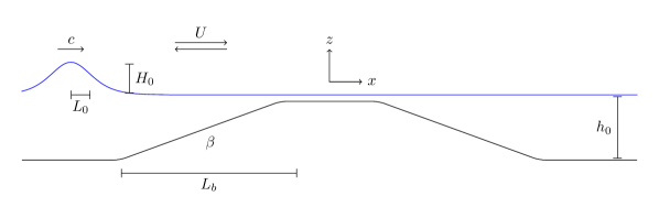
FIG. 1: Schematic showing the (periodic) simulation domain and relevant lengthscales. The blue line represents the water surface and wave profile $\eta$ and the solid black line is the bottom bathymetry $h(x)$. The solitary wave initial condition has a height $H_{0}$ and effective half-width $L_{0}$ and begins with its peak on the far left side, in the middle of flat region of depth $h_{0}$. The initial wave then propagates to the right with phase speed $c$ up the beach with slope $\beta$ until it reaches prebreaking (cf. Sec. II.6). The positive/negative wind speed $U$ corresponds to an onshore/offshore wind forcing.

II.2 Model domain and model parameters

The model domain (Fig. 1) is similar to that of Knowles and Yeh [31] and consists of an initial flat section of length $L_{f}$ at a depth of $h_{0}$ and transitions smoothly at $x=0$ into a planar beach region with constant slope $\beta$ and characteristic beach width $L_{b}\coloneqq h_{0}/\beta$. The bathymetry then smoothly transitions to a flat plateau of length $2L_{f}$ at a depth of $h=0.1h_{0}$ followed by a downward slope with slope $-\beta$. Finally, there is another flat section of length $L_{f}$ at a depth of $h_{0}$ before the domain wraps periodically, which simplifies the boundary conditions.

The initial condition will be a KdV solitary wave with height $H_{0}$ and width $L_{0}$ following Knowles and Yeh [31], and $L_{0}$ will be specified later. The solitary wave begins centered on the left boundary, in between the two flat, deep sections of length $L_{f}$. From the defined dimensional quantities, we specify four nondimensional parameters

$$\varepsilon_{0}\coloneqq\frac{H_{0}}{h_{0}},\qquad\mu_{0}\coloneqq\pqty{\frac{h_{0}}{L_{0}}}^{2},\qquad P_{0}\coloneqq\frac{P}{\rho_{w}gL_{0}}\,,\qquad\gamma_{0}\coloneqq\frac{L_{0}}{L_{b}}\,.$$ (7)

Here, $\varepsilon_{0}$ is the nondimensional initial wave height, $\mu_{0}$ is the square of the nondimensional initial inverse wave width, $P_{0}$ is the nondimensional pressure magnitude (normalized by the initial wave width), and $\gamma_{0}$ is ratio of the initial wave width to the beach width. Note that the wave width-to-beach width ratio $\gamma_{0}$ is related to the beach slope $\beta$ as $\gamma_{0}=\beta/\sqrt{\mu_{0}}$. Together, these four nondimensional parameters control the system’s dynamics.

II.3 Nondimensionalization

We nondimensionalize our system’s variables using the characteristic scales described in Sec. II.2: the initial depth $h_{0}$; the initial wave’s height $H_{0}$; the initial wave’s horizontal lengthscale $L_{0}$; the gravitational acceleration $g$; and the pressure magnitude $P$. Using primes for nondimensional variables, we normalize as Zdyrski and Feddersen [25] did and define

$$\begin{aligned} x&=L_{0}x^{\prime}=h_{0}\frac{x^{\prime}}{\sqrt{\mu_{0}}}\,,\\ z&=h_{0}z^{\prime}\,,\\ t&=\frac{t^{\prime}L_{0}}{\sqrt{gh_{0}}}=\frac{t^{\prime}}{\sqrt{\mu_{0}}}\sqrt{\frac{h_{0}}{g}}\,,\end{aligned}\qquad\begin{aligned} h&=h^{\prime}h_{0}\,,\\ \eta&=H_{0}\eta^{\prime}=h_{0}\varepsilon_{0}\eta^{\prime}\,,\\ \phi&=\phi^{\prime}H_{0}L_{0}\sqrt{\frac{g}{h_{0}}}=\frac{\phi^{\prime}\varepsilon_{0}}{\sqrt{\mu_{0}}}\sqrt{gh_{0}^{3}}\,.\\ \end{aligned}$$ (8)

We later assume the nondimensional parameters $\varepsilon_{0}$, $\mu_{0}$, $\gamma_{0}$, and $P_{0}$ are small to leverage a perturbative analysis. For the constant slope $\beta$ beach profile, the spatial derivative of the bathymetry is also small $\partial_{x^{\prime}}h^{\prime}=\beta/\sqrt{\mu_{0}}=\gamma_{0}\ll 1$ (the factor of $\sqrt{\mu_{0}}$ comes from the different nondimensionalizations of $h$ and $x$). However, perturbation analyses are simplest when all nondimensional variables are $\order{1}$. Therefore, we leverage the two, horizontal lengthscales $L_{0}$ and $L_{b}$ (cf. Sec. II.2) to define a nondimensional, stretched bathymetry $\tilde{h}^{\prime}$ that depends on $x/L_{b}=\gamma_{0}x^{\prime}$ as $\tilde{h}^{\prime}(\gamma_{0}x^{\prime})=h^{\prime}(x^{\prime})$. Then, denoting derivatives with respect to $\gamma_{0}x^{\prime}$ using an overdot, the derivative of $\tilde{h}$ is $\dot{\tilde{h}}^{\prime}\coloneqq\partial_{\gamma_{0}x^{\prime}}\tilde{h}^{\prime}(\gamma_{0}x^{\prime})=\order{1}$, and the small slope becomes explicit as $\partial_{x^{\prime}}h^{\prime}=\gamma_{0}\dot{\tilde{h}}^{\prime}$.

Now, the nondimensional equations take the form

$$0 =\mu_{0}\partialderivative[2]{\phi^{\prime}}{{x^{\prime}}}+\partialderivative[2]{\phi^{\prime}}{{z^{\prime}}} \mbox{\quad on\quad}-1<z^{\prime}<\varepsilon_{0}\eta^{\prime}\,,$$ (9)

$$\partialderivative{\phi^{\prime}}{z^{\prime}} =-\mu_{0}\gamma_{0}\dot{\tilde{h}}^{\prime}\partialderivative{\phi^{\prime}}{x^{\prime}} \mbox{\quad on\quad}z^{\prime}=-\tilde{h}^{\prime}(\gamma_{0}x^{\prime})\,,$$ (10)

$$\partialderivative{\phi^{\prime}}{z^{\prime}} =\mu_{0}\partialderivative{\eta^{\prime}}{t^{\prime}}+\varepsilon_{0}\mu_{0}\partialderivative{\phi^{\prime}}{x^{\prime}}\partialderivative{\eta^{\prime}}{x^{\prime}} \mbox{\quad on\quad}z^{\prime}=\varepsilon_{0}\eta^{\prime}\,,$$ (11)

$$0 =P_{0}\partialderivative{\eta^{\prime}}{x^{\prime}}+\eta^{\prime}+\partialderivative{\phi^{\prime}}{t^{\prime}}+\frac{1}{2}\bqty{\varepsilon_{0}\pqty{\partialderivative{\phi^{\prime}}{x^{\prime}}}^{2}+\frac{\varepsilon_{0}}{\mu_{0}}\pqty{\partialderivative{\phi^{\prime}}{z^{\prime}}}^{2}} \mbox{\quad on\quad}z^{\prime}=\varepsilon_{0}\eta^{\prime}\,.$$ (12)

For the remainder of Sec. II, we remove the primes for clarity.

II.4 Boussinesq equations, multiple-scale expansion, and vKdV–Burgers equation

We follow the conventional Boussinesq equation derivation presented in, e.g., Mei et al. [53] or Ablowitz [54]. The two modifications we include are the weakly sloping bottom, similar to the treatment in Johnson [43] and Mei et al. [53], and the inclusion of a pressure forcing like that of Zdyrski and Feddersen [25]. However, the joint contributions of both pressure and shoaling are new. For the sake of brevity, we only detail the relevant differences here, but we still treat the derivation formally to ensure a proper ordering of small terms and obtain the parameters’ validity ranges. First, we expand the velocity potential in a Taylor series about the bottom $z=-h(x)$ as

$$\phi(x,z,t)=\sum_{n=0}^{\infty}\bqty{z+\tilde{h}(\gamma_{0}x)}^{n}\phi_{n}(x,t)\,.$$ (13)

Substituting this expansion into the incompressibility Eq. 9 and bottom boundary condition 10 and assuming $\mu_{0}\ll 1$ gives $\phi$ as a function of the velocity potential evaluated at the bottom $\varphi\coloneqq\phi_{0}$. If we further assume that the bottom is very weakly sloping $\gamma_{0}\sim\mu_{0}\ll 1$, this simplifies to

$$\phi=\varphi-\mu_{0}\frac{1}{2}(z+\tilde{h})^{2}\partial_{x}^{2}\varphi+\order{\mu_{0}^{2},\gamma_{0}^{2},\gamma_{0}\mu_{0}}\,.$$ (14)

Note that the assumption $\gamma_{0}\sim\mu_{0}\ll 1$ implies a moderate slope $\beta=\gamma_{0}\sqrt{\mu_{0}}\sim\mu_{0}^{3/2}$ and is used by several other authors [43, 45, 31]. For reference, if $\mu_{0}=\gamma_{0}=0.1$, then this implies a physically realistic $\beta=0.03$.

Substituting this $\phi$ expansion 14 into the kinematic boundary condition 11 and dynamic boundary condition 12 yields Boussinesq-type equations with a pressure-forcing term

$$\partial_{t}\eta+\pqty{\tilde{h}+\varepsilon_{0}\eta}\partial^{2}_{x}\varphi\ +\pqty{\gamma_{0}\dot{\tilde{h}}+\varepsilon_{0}\partial_{x}\eta}\partial_{x}\varphi-\mu_{0}\frac{1}{6}\tilde{h}^{3}\partial^{4}_{x}\varphi=\order{\mu_{0}^{2},\gamma_{0}^{2},\gamma_{0}\mu_{0}}\,,$$ (15)

$$P_{0}\partial_{x}\eta+\eta+\partial_{t}\varphi-\frac{1}{2}\mu_{0}\tilde{h}^{2}\partial^{2}_{x}\partial_{t}\varphi+\frac{1}{2}\varepsilon_{0}\pqty{\partial_{x}\varphi}^{2}=\order{\mu_{0}^{2},\gamma_{0}^{2},\gamma_{0}\mu_{0}}\,.$$ (16)

Note that replacing $\tilde{h}$ with the total depth $h_{\text{total}}=\tilde{h}+\varepsilon_{0}\eta$ shows that these are equivalent to the flat-bottomed Boussinesq equations with $h_{\text{total}}=1+\varepsilon_{0}\eta$. In other words, any sloping-bottom terms $\dot{\tilde{h}}$ only appear in the combination $\partial_{x}h_{\text{total}}=\gamma_{0}\dot{\tilde{h}}+\varepsilon_{0}\partial_{x}\eta$. This is expected since the only sloping-bottom term $\mu_{0}\gamma_{0}\dot{\tilde{h}}\partial_{x}\phi$ in the governing equations 9, 10, 11, and 12 was dropped when we neglected terms of $\order{\mu_{0}^{2},\gamma_{0}^{2},\gamma_{0}\mu_{0}}$.

Since the bathymetry varies on the slow scale $x/\gamma_{0}$, we expand our system in multiple spatial scales $x_{n}=\gamma_{0}^{n}x$ for $n=0,1,2,\ldots$, so the derivatives become

$$\partialderivative{x}\to\partialderivative{x_{0}}+\gamma_{0}\partialderivative{x_{1}}+\ldots\,,$$ (17)

and the bathymetry is a function of the long spatial scale $\tilde{h}=\tilde{h}(x_{1})$. Then, we expand $\eta$ and $\varphi$ in asymptotic series of $\varepsilon_{0}$

$$\eta(x,t)\to\sum_{k=0}^{\infty}\varepsilon_{0}^{k}\eta_{k}(t,x_{0},x_{1},\ldots)\,,\qquad\varphi(x,t)\to\sum_{k=0}^{\infty}\varepsilon_{0}^{k}\varphi_{k}(t,x_{0},x_{1},\ldots)\,.$$ (19)

Similar to Johnson [43], we replace $x_{0}$ and $t$ with left- and right-moving coordinates translating with speed $\tilde{c}(x_{1})$ dependent on the stretched coordinate $x_{1}$:

$$\xi_{+}=-t+\int^{x_{0}}\frac{dx^{\prime}_{0}}{\tilde{c}(\gamma_{0}x^{\prime}_{0})}\,,\qquad\xi_{-}=t+\int^{x_{0}}\frac{dx^{\prime}_{0}}{\tilde{c}(\gamma_{0}x^{\prime}_{0})}\,.$$ (20)

Then, we replace the derivatives $\partial_{t}$ and $\partial_{x_{0}}$ with

$$\partialderivative{t}=\partialderivative{\xi_{-}}-\partialderivative{\xi_{+}}\,,\qquad\partialderivative{x_{0}}=\frac{1}{\tilde{c}}\pqty{\partialderivative{\xi_{-}}+\partialderivative{\xi_{+}}}\,.$$ (21)

Now, we will assume that $\varepsilon_{0}\sim P_{0}\sim\mu_{0}\ll 1$ and follow the standard multiple-scale technique [53, 54]. The order-one terms $\order{\varepsilon_{0}^{0}}$ from Eqs. 15 and 16 yield wave equations for $\phi_{0}$ and $\eta_{0}$

$$\partialderivative{\phi_{0}}{\xi_{+}}{\xi_{-}}=0\,,\qquad\partialderivative{\eta_{0}}{\xi_{+}}{\xi_{-}}=0\,,$$ (23)

with right-moving solutions

$$\varphi_{0}=f_{0}(\xi_{+},x_{1})\mbox{\quad and\quad}\eta_{0}=\partial_{\xi_{+}}f_{0}(\xi_{+},x_{1})\,,$$ (24)

propagating with the slowly varying, linear shallow-water phase speed $\tilde{c}(x_{1})=\sqrt{\tilde{h}(x_{1})}$. Continuing to $\order{\varepsilon_{0}}$ of the asymptotic expansion gives

$$\begin{split}&-\partialderivative{\eta_{1}}{\xi_{+}}+\partialderivative{\eta_{1}}{\xi_{-}}+\partialderivative[2]{\varphi_{1}}{\xi_{+}}+2\partialderivative{\varphi_{1}}{\xi_{+}}{\xi_{-}}+\partialderivative[2]{\varphi_{1}}{\xi_{-}}=-2\frac{\gamma_{0}}{\varepsilon_{0}}\tilde{c}\partialderivative{\varphi_{0}}{\xi_{+}}{x_{1}}+\frac{\gamma_{0}}{\varepsilon_{0}}\partialderivative{\tilde{c}}{x_{1}}\partialderivative{\varphi_{0}}{\xi_{+}}\\ &\qquad-\frac{1}{\tilde{c}^{2}}\eta_{0}\partialderivative[2]{\varphi_{0}}{\xi_{+}}-\frac{\gamma_{0}}{\varepsilon_{0}}\frac{\dot{\tilde{h}}}{\tilde{c}}\partialderivative{\varphi_{0}}{\xi_{+}}-\frac{1}{\tilde{c}^{2}}\partialderivative{\eta_{0}}{\xi_{+}}\partialderivative{\varphi_{0}}{\xi_{+}}+\frac{\mu_{0}}{\varepsilon_{0}}\tilde{h}\frac{1}{6}\partialderivative[4]{\varphi_{0}}{\xi_{+}}\,,\end{split}$$ (25)

$$\begin{split}&\eta_{1}-\partialderivative{\varphi_{1}}{\xi_{+}}+\partialderivative{\varphi_{1}}{\xi_{-}}=-\frac{P_{0}}{\varepsilon_{0}}\frac{1}{\tilde{c}}\partialderivative{\eta_{0}}{\xi_{+}}-\frac{1}{2}\frac{\mu_{0}}{\varepsilon_{0}}\tilde{h}\frac{\partial^{3}\varphi_{0}}{\partial^{3}\xi_{+}}-\frac{1}{2\tilde{c}^{2}}\pqty{\partialderivative{\varphi_{0}}{\xi_{+}}}^{2}\,.\end{split}$$ (26)

Eliminating $\eta_{1}$ from these equations gives

$$4\partialderivative{\phi_{1}}{\xi_{+}}{\xi_{-}}=-2\frac{\gamma_{0}}{\varepsilon_{0}}\tilde{c}\partialderivative{\eta_{0}}{x_{1}}-\frac{\gamma_{0}}{\varepsilon_{0}}\partialderivative{\tilde{c}}{x_{1}}\eta_{0}-3\frac{1}{\tilde{c}^{2}}\eta_{0}\partialderivative{\eta_{0}}{\xi_{+}}-\frac{1}{3}\frac{\mu_{0}}{\varepsilon_{0}}\tilde{c}^{2}\partialderivative[3]{\eta_{0}}{\xi_{+}}-\frac{1}{\tilde{c}}\frac{P_{0}}{\varepsilon_{0}}\partialderivative[2]{\eta_{0}}{\xi_{+}}\,.$$ (27)

The left-hand operator $\partial^{2}/\partial\xi_{-}\partial\xi_{+}$ is the same as the $\order{1}$ differential operator 21. Therefore, the right-hand side must vanish to prevent $\phi_{1}$ from developing secular terms. Thus, the right-hand side becomes the variable-coefficient Korteweg–de Vries–Burgers (vKdV–Burgers) equation

$$\frac{\gamma_{0}}{\varepsilon_{0}}\tilde{c}\partialderivative{\eta_{0}}{x_{1}}+\frac{1}{2}\frac{\gamma_{0}}{\varepsilon_{0}}\partialderivative{\tilde{c}}{x_{1}}\eta_{0}+\frac{3}{2}\frac{1}{\tilde{c}^{2}}\eta_{0}\partialderivative{\eta_{0}}{\xi_{+}}+\frac{1}{6}\frac{\mu_{0}}{\varepsilon_{0}}\tilde{c}^{2}\partialderivative[3]{\eta_{0}}{\xi_{+}}+\frac{1}{2\tilde{c}}\frac{P_{0}}{\varepsilon_{0}}\partialderivative[2]{\eta_{0}}{\xi_{+}}=0\,.$$ (28)

Finally, multiplying Eq. 28 by $\varepsilon_{0}$, adding the $\order{1}$ differential equation $\partial_{\xi_{-}}\eta_{0}=0$ derived from Eq. 21, and transforming back to the original, nondimensional variables $x$ and $t$ yields

$$\partialderivative{\eta_{0}}{t}+c\partialderivative{\eta_{0}}{x}+\frac{1}{2}\partialderivative{c}{x}\eta_{0}+\frac{3}{2}\varepsilon_{0}\frac{1}{c}\eta_{0}\partialderivative{\eta_{0}}{x}+\frac{1}{6}\mu_{0}c^{5}\partialderivative[3]{\eta_{0}}{x}+\frac{1}{2}P_{0}c\partialderivative[2]{\eta_{0}}{x}=0\,.$$ (29)

This vKdV–Burgers equation represents an analytically simple system for studying the effects of wind-forcing and shoaling. In the absence of wind-forcing ($P_{0}=0$), it reduces to the variable-coefficient KdV equation [46], while it simplifies to the constant-coefficient KdV–Burgers equation in the case of flat bathymetry ($c=1$) [25]. The formal derivation revealed the depth-dependent $c$ factor in the wind-forced $P_{0}$ term which was absent in the flat-bottomed case. The pressure term $P_{0}\partial^{2}_{x}\eta_{0}$ functions as a damping, positive viscosity for offshore $P_{0}<0$ wind, making Eq. 29 a (forward) vKdV–Burgers equation. Conversely, onshore $P_{0}>0$ wind causes a growth-inducing, negative viscosity giving the backward vKdV–Burgers equation. Though the backward, constant-coefficient KdV–Burgers equation is ill posed in the sense of Hadamard [55], this is irrelevant here owing to the finite time the wave takes to reach the beach.

II.5 Initial conditions

Our initial condition will be the solitary-wave solutions of the unforced ($P_{0}=0$), flat-bottom KdV equation. These waves balance the KdV equation’s nonlinearity $\eta_{0}\partial_{x}\eta_{0}$ and dispersion $\partial_{x}^{3}\eta_{0}$ terms, propagate without changing shape, and require that the height $H_{0}$ and width $L_{0}$ satisfy the constraint $H_{0}L_{0}^{2}=\text{constant}$. Therefore, we now fix the previously unspecified $L_{0}$ by choosing $\mu_{0}=(3/4)\varepsilon_{0}$ so $L_{0}$ acts like an effective half-width for the solitary wave initial condition [53]

$$\eta_{0}=\sech^{2}\pqty{x}\,.$$ (30)

While the unforced KdV equation also possesses periodic solutions called cnoidal waves, we only consider solitary waves here.

II.6 Convective breaking criterion

The asymptotic assumptions used to derive the vKdV–Burgers equation 29 fail when the wave gets too large. Therefore, we require a condition to determine when the simulations should stop. Brun and Kalisch [35] defined a convective breaking condition for solitary waves on a flat-bottom depending on the surface water velocity $u_{s}(x,t)$ and the phase speed $c$ using the local Froude number $\operatorname{Fr}\coloneqq\varepsilon_{0}u_{s}(x,t)/c(t)$, with the $\varepsilon_{0}$ coming from nondimensionalization. Convective breaking occurs wherever $\max_{x}(\operatorname{Fr})=1$, where $\max_{x}$ represents the maximum over $x$. However, when the Froude number approaches the breaking value of unity, our weakly nonlinear asymptotic assumption used to derive the vKdV–Burgers equation is violated. Thus, we instead stop our simulations at the smaller prebreaking Froude number $\operatorname{Fr}_{\text{pb}}\coloneqq 1/3$ and define the “prebreaking” time $t_{\text{pb}}$ as the first time such that $\max_{x}(\operatorname{Fr})=\operatorname{Fr}_{\text{pb}}\coloneqq 1/3$. Likewise, we define $x_{\text{pb}}$ as the location where $\operatorname{Fr}=\operatorname{Fr}_{\text{pb}}$, which will be very near the wave peak.

As the solitary wave propagates on a slope, the wave evolves over time and the phase speed $c$ can be ambiguous. One option is to use the adiabatic approximation derived by the authors of [45] for unforced solitary waves on very gentle slopes

$$c_{\text{adi}}(t)=\sqrt{h[x_{\text{peak}}(t)]}\pqty{1+\frac{\varepsilon_{0}}{2}\frac{\eta[x_{\text{peak}}(t)]}{h[x_{\text{peak}}(t)]}}\,,$$ (31)

with $x_{\text{peak}}$ the location of the wave peak. Alternatively, Derakhti et al. [33] used large eddy simulations to numerically investigate unforced solitary wave breaking on slopes ranging from $\beta=$0.20.005$$ for two different forms of $c$. They found wave breaking at $\max_{x}(\operatorname{Fr})=0.85$ when using the speed of the numerically tracked wave peak $c_{\text{peak}}$. However, they also found that the shallow-water approximation $c_{\text{shallow}}=\sqrt{h(x_{\text{peak}})+\varepsilon_{0}\eta(x_{\text{peak}})}$ [equivalent to $c_{\text{adi}}$ to $\order{\varepsilon_{0}^{2}}$] was within $15\text{\,}\mathrm{\char 37\relax}$ of $c_{\text{peak}}$ near breaking. Therefore, we will use Eq. 31 for $c(t)$ owing to its simplicity and theoretical foundation. Finally, though these studies all considered unforced solitary waves, our results will show that $c_{\text{adi}}$ varies approximately $3\text{\,}\mathrm{\char 37\relax}$ across pressure magnitudes $P_{0}$ for our simulations, so this approximation is valid.

We still need an expression for the wave velocity at the surface $u_{s}(x,t)$, which we now derive by modifying the example of Brun and Kalisch [35] to include sloping bathymetry and pressure forcing. Combining the vKdV–Burgers equation 29 and kinematic boundary condition 15 eliminates $\partial_{t}\eta$ yielding

$$\begin{split}&\tilde{c}^{2}\partialderivative[2]{\varphi}{x}-\tilde{c}\partialderivative{\eta}{x}+\varepsilon_{0}\pqty{\eta\partialderivative[2]{\varphi}{x}+\partialderivative{\eta}{x}\partialderivative{\varphi}{x}-\frac{3}{2}\frac{1}{\tilde{c}}\eta\partialderivative{\eta}{x}}-P_{0}\frac{1}{2}\tilde{c}\partialderivative[2]{\eta}{x}\\ &\qquad-\mu_{0}\pqty{\frac{1}{6}\tilde{c}^{6}\partialderivative[4]{\varphi}{x}+\frac{1}{6}\tilde{c}^{5}\partialderivative[3]{\eta}{x}}+\gamma_{0}\pqty{2\tilde{c}\dot{\tilde{c}}\partialderivative{\varphi}{x}-\frac{1}{2}\eta\dot{\tilde{c}}}=0\,.\end{split}$$ (32)

Here, $\dot{\tilde{c}}\coloneqq\partial_{x_{1}}\tilde{c}(x_{1})=\order{1}$ in analogy to the previously defined $\dot{\tilde{h}}$. Assuming an ansatz

$$\partialderivative{\varphi}{x} =\frac{1}{\tilde{c}}\eta+\varepsilon_{0}A(x,t)+\gamma_{0}B(x,t)+\mu_{0}C(x,t)+P_{0}D(x,t)$$ (33)

$$\implies\partialderivative[2]{\varphi}{x} =\frac{1}{\tilde{c}}\partialderivative{\eta}{x}+\varepsilon_{0}\partialderivative{A}{x}+\gamma_{0}\pqty{\partialderivative{B}{x}-\frac{1}{\tilde{c}^{2}}\eta\dot{\tilde{c}}}+\mu_{0}\partialderivative{C}{x}+P_{0}\partialderivative{D}{x}\,,$$ (34)

we insert Eqs. 33 and 34 into Eq. 32, drop terms of $\order{\varepsilon_{0}^{2}}$ and solve for $A$, $B$, $C$, and $D$ by using the independence of $\varepsilon_{0}$, $\gamma_{0}$, $\mu_{0}$, and $P_{0}$:

$$A=-\frac{1}{4\tilde{c}^{3}}\eta^{2}\,,\qquad B=-\frac{1}{2\tilde{c}^{2}}\int^{x}_{-\infty}\eta(x^{\prime})\dot{\tilde{c}}(\gamma_{0}x^{\prime})dx^{\prime}\,,\qquad C=\frac{\tilde{c}^{3}}{3}\partialderivative[2]{\eta}{x}\,,\qquad D=\frac{1}{2\tilde{c}}\partialderivative{\eta}{x}\,.$$ (36)

Note that $A$ represents the nonlinear contribution, $B$ the effect of shoaling, $C$ the dispersive effect, and $D$ the pressure forcing. Finally, the Taylor expansion of $\phi(x,z)$ Eq. 14 gives the fluid velocity at the surface $u_{s}(x,t)$ using $u=\partial_{x}\phi$ evaluated at $z=\varepsilon_{0}\eta$:

$$\begin{split}u_{s}(x,t)&=\partial_{x}\varphi-\mu_{0}\frac{1}{2}\tilde{c}^{4}\partial^{3}_{x}\varphi\\ &=\frac{1}{\tilde{c}}\eta-\varepsilon_{0}\frac{1}{4\tilde{c}^{3}}\eta^{2}+P_{0}\frac{1}{2\tilde{c}}\partialderivative{\eta}{x}-\mu_{0}\frac{\tilde{c}^{3}}{6}\partialderivative[2]{\eta}{x}-\gamma_{0}\frac{1}{2\tilde{c}^{2}}\int_{-\infty}^{x}\eta(x^{\prime})\dot{\tilde{c}}(\gamma_{0}x^{\prime})dx^{\prime}\,.\end{split}$$ (37)

Therefore, the Froude number is calculated as

$$\operatorname{Fr}\coloneqq\frac{\varepsilon_{0}u_{s}(x_{\text{peak}},t_{\text{peak}})}{\sqrt{h(x_{\text{peak}})}}\pqty{1+\frac{\varepsilon_{0}}{2}\frac{\eta(x_{\text{peak}})}{h(x_{\text{peak}})}}^{-1}\,,$$ (38)

with $u_{s}(x,t)$ given by Eq. 37. Equation 38 demonstrates that the choice of $\operatorname{Fr}_{\text{pb}}=1/3$ keeps the problem in the correct asymptotic regime. Our simulated waves will reach prebreaking in depths of $h(x_{\text{pb}})=$0.590.72$$, so Eqs. 37 and 38 show that $\operatorname{Fr}_{\text{pb}}=1/3$ corresponds to a dimensional $H(x_{\text{pb}})/h(x_{\text{pb}})\approx\operatorname{Fr}_{\text{pb}}/\sqrt{h(x_{\text{pb}})}=$0.390.43$$. Considering an asymptotic regime around $\varepsilon_{0}$ of $\varepsilon_{0}^{3/2}$ to $\varepsilon_{0}^{1/2}$, or $0.0890.45$, we see that $H(x)/h(x)$ remains in the asymptotic regime.

II.7 Numerics

TABLE 1: Range of nondimensional parameters simulated.

Parameter	Range
$\varepsilon_{0}$	0.2
$\mu_{0}$	0.15
$\absolutevalue{P/(\rho_{w}gL_{0}\varepsilon_{0})}$	0, 0.00625, 0.0125, 0.025, 0.05
$\beta$	0.01, 0.015, 0.02, 0.025

The vKdV–Burgers equation 29 lacks analytic, solitary-wave-type solutions, so we solve it numerically using a third-order explicit Runge-Kutta adaptive time stepper with the error controlled by a second-order Runge-Kutta method as implemented in SciPy [56]. The domain’s deep, flat regions have length $L_{f}=20L_{0}$. Therefore, the spatial domain’s entire, periodic width $L_{x}$ varies between $108$ and $150$, depending on the slope $\beta$. We discretize the spatial domain using a fourth-order finite difference method with $N_{x}=2^{2}\lfloor L_{x}/0.025/2^{2}\rceil$ points which yields a grid spacing of $dx=L_{x}/N_{x}\approx 0.025$ and ensures that the grid can be refined by two steps. We employ adaptive time stepping to keep the relative error below ${10}^{-3}$ and the absolute error below ${10}^{-6}$ at each step. For all cases, the average time step is $\Delta t\approx$2\text{\times}{10}^{-4}$$. The pressure is initially turned off until the solitary wave is one unit (i.e., a half-width $L_{0}$) away from the start of the beach slope. The pressure is linearly ramped up to its full value over the time the wave takes to cross a full-width $2L_{0}$. We included a hyperviscosity $\nu_{4}\partial_{x}^{4}\eta_{0}$ with $\nu_{4}=$1\text{\times}{10}^{-5}$$ for numerical stability [57]. Finally, we only considered solitary waves, as mentioned previously, because cnoidal wave trains require spin-up and damping since we only consider prebreaking waves.

We validated the solver against the unforced, flat-bottom analytical solution and had a normalized root-mean-square error of $1.6\text{\times}{10}^{-4}$ after nondimensional time $t=50$ (the longest simulation time) as well as a normalized wave height change of $1-\bqty{\max(\eta_{0})-\min(\eta_{0})}/\allowbreak\bqty{\max(\eta^{(0)}_{0})-\min(\eta^{(0)}_{0})}=$1.4\text{\times}{10}^{-4}$$. To verify the numerical convergence on our nominal (fine) grid size, we also ran the simulation on a medium grid and a fine grid, each with a refinement ratio of $2$. We then calculated the Romberg interpolation [58] and compared each grid’s normalized root-mean-square error with respect to this interpolation to yield a grid refinement index ($GCI$) [59] for the unforced case with the steepest $\beta=0.025$ and shallowest $\beta=0.01$ slopes. Both slopes had a convergence order $p>$2.1$$ which yielded grid convergence indices indices $GCI_{\text{nominal,medium}}<$3\text{\times}{10}^{-4}$$ and $GCI_{\text{medium,coarse}}<$8\text{\times}{10}^{-4}$$ much less than unity and implying that the results are grid-converged. Furthermore, the profiles for all times until prebreaking were nearly identical to the simulations of Knowles and Yeh [31] for an unforced solitary wave shoaling on a slope. Finally, the simulation reproduced the finding of Knowles and Yeh [31] that small waves ($\varepsilon_{0}\ll 1$) on weak slopes ($\gamma_{0}\ll 1$) yield Green’s Law for the wave height $H(x)\coloneqq\max_{t}(\eta)\propto h(x)^{1/4}$ (with $\max_{t}$ the maximum over time $t$), while moderate waves ($\varepsilon_{0}<1$) on very weak slopes ($\gamma_{0}\lll 1$) give Miles’ adiabatic law $H(x)\propto h(x)^{-1}$ [60].

The vKdV–Burgers equation 28 is determined by two nondimensional parameter combinations: the pressure term $P_{0}/\varepsilon_{0}$ and the shoaling term $\gamma_{0}/\varepsilon_{0}$. Recall that the dispersive term $\mu_{0}/\varepsilon_{0}$ is a redundancy which we fixed by specifying $L_{0}$ (cf. Sec. II.5). We investigate this two-dimensional parameter space by choosing $\varepsilon_{0}=0.2$ and $\mu_{0}=0.15$ and varying the beach slope $\beta=$0.010.025$$ and pressure $\absolutevalue{P}=$00.05$$ (cf. Sec. IV.1 for a discussion of the size of $P$). This yields a total of $36$ simulations (Table 1). Note that Eq. 28 demonstrates changing $\varepsilon_{0}\to\lambda\varepsilon_{0}$ is equivalent to $\gamma_{0}\to\gamma_{0}/\lambda$ in the wave’s comoving reference frame. Therefore, solutions for waves with different initial heights $\varepsilon_{0}$ can be generated from our solutions to the vKdV–Burgers equation in the laboratory frame Eq. 29 by scaling the height, boosting, and adjusting $\gamma_{0}$. Note the asymptotic expansion assumed $P_{0}\sim\varepsilon_{0}$, or $P/(\rho_{w}gL_{0}\varepsilon_{0})\sim 1$, but the pressure values we are using (Table 1) are smaller than unity. Nevertheless, multiple-scale expansions are often accurate outside their parameters’ validity ranges and this constraint would be satisfied asymptotically for smaller values of $\varepsilon_{0}$.

II.8 Shape statistics

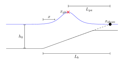
FIG. 2: Schematic showing the definition of the prebreaking zone and shore locations. The blue line represents the water surface and wave profile $\eta$ at prebreaking and the solid black line is the bottom bathymetry $h(x)$. The bathymetry consists of a flat region of depth $h_{0}$, a sloping region, and a shallow plateau. The shoreline $x_{\text{shore}}$ (black dot) is the location where the bathymetry would intersect the still water level if it had a constant slope (dashed line). The beach width $L_{b}$ is the distance from the toe of the beach slope to $x_{\text{shore}}$ and the prebreaking point $x_{\text{pb}}$ is the location on the wave where $\operatorname{Fr}=\operatorname{Fr}_{\text{pb}}$, which will be very near the wave peak. The prebreaking zone width $L_{\text{pz}}$ is the distance from $x_{\text{pb}}$ to $x_{\text{shore}}$.

While previous studies investigated shoaling’s effect on wave-breaking location, we will theoretically examine the combined influences of both wind and shoaling on wave location $x_{\text{pb}}$ at prebreaking $t_{\text{pb}}$ (Sec. II.6). To estimate how $x_{\text{pb}}$ changes, we first calculate the shoreline $x_{\text{shore}}$ as the location where the bathymetry would intersect $z=0$ if it had a constant slope $\beta$ without our shallow plateau (Fig. 2). Then, we calculate the prebreaking zone width as $L_{\text{pz}}\coloneqq x_{\text{pb}}-x_{\text{shore}}$. For a given beach slope $\beta$, we will analyze the change in the prebreaking zone width relative to the unforced case $\Delta L_{\text{pz}}\coloneqq L_{\text{pz}}-\evaluated{L_{\text{pz}}}_{P=0}$ normalized by the unforced prebreaking zone width $\evaluated{L_{\text{pz}}}_{P=0}$. This bulk statistic $\Delta L_{\text{pz}}/(\evaluated{L_{\text{pz}}}_{P=0})$ determines the variance in prebreaking locations as a fractional change of the prebreaking zone width.

Additionally, since we wish to analyze the effect of wind and shoaling on wave shape, we will investigate four shape statistics that vary as the wave propagates. The first three are local shape parameters defined at each location $x$. First, we directly examine the maximum Froude number $\max_{t}(\operatorname{Fr})$ expressed in Eq. 38. Second, we investigate the maximum height relative to the local water depth $\max_{t}(\eta)/h(x)$ at each location $x$. Third, we consider the maximum slope $\max_{t}(\absolutevalue{\partial\eta/\partial x})$. Both the relative height and maximum slope contribute to the convective breaking criterion $\max_{x}(\operatorname{Fr})=\operatorname{Fr}_{\text{pb}}$. Finally, we introduce a bulk shape parameter, the full width of the wave at half of the wave’s maximum (FWHM) $L_{W}(t)$ normalized by the local water depth $h(x)$. For our unforced KdV solitary wave initial condition 30, the FWHM divided by the initial depth is $L_{W}/h_{0}=2\cosh^{-1}(\sqrt{2})/\sqrt{\mu_{0}}$. We seek to compare this bulk shape parameter defined at each point in time $t$ with the local parameters defined at each point in space. Therefore, we define $L_{W}(x)=L_{W}[t_{\text{peak}}(x)]$ at the time $t_{\text{peak}}(x)$ when the wave peak passes location $x$.

III Results

Now, we use the results of the numerical simulations to investigate the effect of wind on solitary wave shoaling and shape. We will present shape statistics (Sec. II.8) for the 20 different runs (Table 1) to detail the wave-shape changes and prebreaking behavior across the parameter space. For the remainder of the paper we will return to dimensional variables.

III.1 Profiles of shoaling solitary waves with wind

((a))

((b))

((c))

((d))

((e))

((f))

((g))

((h))

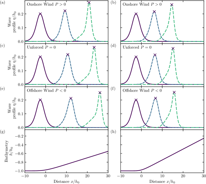
FIG. 3: Shoaling solitary-wave $\eta$ evolution under [LABEL:sub@fig:snapshots_solitary:a,LABEL:sub@fig:snapshots_solitary:b] onshore $P>0$, [LABEL:sub@fig:snapshots_solitary:c,LABEL:sub@fig:snapshots_solitary:d] unforced $P=0$, and [LABEL:sub@fig:snapshots_solitary:e,LABEL:sub@fig:snapshots_solitary:f] offshore $P<0$ wind-induced surface pressure versus nondimensional distance $x/h_{0}$ as the wave propagates up the [LABEL:sub@fig:snapshots_solitary:g,LABEL:sub@fig:snapshots_solitary:h] planar bathymetry. The profile times shown depend on the Froude number 38 and therefore vary between the panels. The first profile (purple) occurs when the peak is located at $x=-L_{0}$ where the pressure begins turning on and the time is defined so $t=0$ here. The last profile (green) occurs when the convective prebreaking condition $\max_{x}(\operatorname{Fr})=\operatorname{Fr}_{\text{pb}}=1/3$ is met (cf. Sec. II.6), and the middle profile (blue) occurs at a time halfway between the first and last profiles. Both columns have $\varepsilon_{0}=0.2$ and $\mu_{0}=0.15$, and [LABEL:sub@fig:snapshots_solitary:a,LABEL:sub@fig:snapshots_solitary:e] the left-column forced cases have $\absolutevalue{P/(\rho_{w}gL_{0}\varepsilon_{0})}=0.05$ and $\beta=0.015$ while [LABEL:sub@fig:snapshots_solitary:b,LABEL:sub@fig:snapshots_solitary:f] the right-column forced cases use $\absolutevalue{P/(\rho_{w}gL_{0}\varepsilon_{0})}=0.025$ and $\beta=0.025$. The $\times$’s denote the locations with the highest Froude number 38, and the $\times$’s on the last profiles (green) are the prebreaking locations $x_{\text{pb}}$. We only display a subset of the full spatial domain. Note that the aspect ratio is chosen to highlight the wind’s effect on the shoaling solitons.

First, we qualitatively investigate the effect of varying pressures $P$ and bathymetric slopes $\beta$ on solitary-wave shoaling by examining the wave profile $\eta/h_{0}$, normalized by the initial depth $h_{0}$, at three different times $t$ (Fig. 3) corresponding to when the solitary wave first feels the slope ($t=0$), the time of prebreaking ($t=t_{\text{pb}}$), and half-way between ($t=t_{\text{pb}}/2$). Note that these $t=0$ wave profiles (purple in Fig. 3) are nearly identical to the $\sech^{2}(x/L_{0})$ initial condition 30 since the waves have only propagated over a flat bottom [Figs. 3(g) and 3(h)] and the pressure has not yet been turned on. Halfway to prebreaking ($t=t_{\text{pb}}/2$, blue), the solitary wave has grown through shoaling with a steeper front face ($+x$ side) and increased asymmetry for all $P$ and $\beta$. At the time of prebreaking ($t=t_{\text{pb}}$, green) the solitary wave has increased in height, steepened, and gained a substantial rear shelf for all $P$ and $\beta$. These changes are likely even larger for waves propagating to full wave breaking ($\operatorname{Fr}\approx 1$). The generation of rear shelves by shoaling solitary waves as in Fig. 3 was first calculated by Miles [45] and resulted from the mass shed by the $\sech^{2}$ wave as it narrowed. Onshore wind ($P>0$) reinforces the shoaling-based wave growth and yields relatively narrow peak widths for both $\beta$ [Figs. 3(a) and 3(b)]. In contrast, offshore wind ($P<0$) reduces the wave shoaling, but results in wider peak widths [Figs. 3(e) and 3(f)]. For instance, the width at prebreaking on the milder slope $\beta=0.015$ is $L_{W}/h(x)=$3.75$$ under onshore winds and $L_{W}/h(x)=$4.26$$ under offshore winds. These differences in wave-shoaling result in the offshore-forced ($P<0$) solitary wave reaching prebreaking ($x_{\text{pb}}$, $\times$’s in Fig. 3) farther onshore (shallower water) than the onshore-forced ($P>0$) solitary wave. For the $\beta=0.015$ case, the onshore-forced wave reaches prebreaking at $x_{\text{pb}}/h_{0}=$20.8$$ while the offshore-forced wave reaches prebreaking farther offshore at $x_{\text{pb}}/h_{0}=$26.1$$. Similarly, the larger beach slope [$\beta=0.025$, Figs. 3(b), 3(d), and 3(f)] causes waves to reach $x_{\text{pb}}$ in less horizontal distance, though they prebreak in shallow water than the milder beach slope ($\beta=0.015$) waves. For the unforced case, the $\beta=0.015$ wave prebreaks at $x_{\text{pb}}/h_{0}=$23.3$$ while the steeper beach $\beta=0.025$ causes prebreaking at $x_{\text{pb}}/h_{0}=$15.2$$. At $t=t_{\text{pb}}$, the rear shelf is wider and extends higher up the rear face for offshore winds [$\approx 0.1h_{0}$ in Fig. 3(e)] than for onshore winds [$\approx 0.07h_{0}$ in Fig. 3(a)]. Again, we expect these differences to be even larger for fully breaking waves ($\operatorname{Fr}\approx 1$). As the control case, the unforced ($P=0$) solitary wave has $x_{\text{pb}}$ located between the onshore and offshore wind cases with an intermediate rear shelf. Finally, the milder slope ($\beta=0.015$) has a sharper, more pronounced rear shelf while the steeper slope ($\beta=0.025$) has a more gently sloping rear shelf.

((a))

((b))

((c))

((d))

((e))

((f))

((g))

((h))

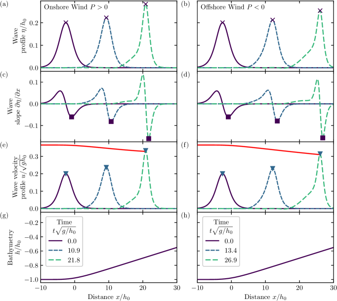
FIG. 4: Shoaling solitary-wave [LABEL:sub@fig:snapshots_solitary_slope_velocity:a,LABEL:sub@fig:snapshots_solitary_slope_velocity:b] nondimensional profile $\eta/h_{0}$, [LABEL:sub@fig:snapshots_solitary_slope_velocity:c,LABEL:sub@fig:snapshots_solitary_slope_velocity:d] slope $\partial\eta/\partial x$, and [LABEL:sub@fig:snapshots_solitary_slope_velocity:e,LABEL:sub@fig:snapshots_solitary_slope_velocity:f] nondimensional wave velocity profile $u/\sqrt{gh_{0}}$ under [LABEL:sub@fig:snapshots_solitary_slope_velocity:a,LABEL:sub@fig:snapshots_solitary_slope_velocity:c,LABEL:sub@fig:snapshots_solitary_slope_velocity:e] onshore and [LABEL:sub@fig:snapshots_solitary_slope_velocity:b,LABEL:sub@fig:snapshots_solitary_slope_velocity:d,LABEL:sub@fig:snapshots_solitary_slope_velocity:f] offshore wind-induced surface pressure as the wave propagates up the [LABEL:sub@fig:snapshots_solitary_slope_velocity:g,LABEL:sub@fig:snapshots_solitary_slope_velocity:h] planar bathymetry. All panels use the same [LABEL:sub@fig:snapshots_solitary_slope_velocity:g,LABEL:sub@fig:snapshots_solitary_slope_velocity:h] bathymetry and differ only in the sign of the pressure forcing. Values are shown versus nondimensional distance $x/h_{0}$ for $\varepsilon_{0}=0.2$, $\mu_{0}=0.15$, $\absolutevalue{P/(\rho_{w}gL_{0}\varepsilon_{0})}=0.05$, $\beta=0.015$, and nondimensional times $t\sqrt{gh}/L_{0}$ indicated in the legends. The red lines in [LABEL:sub@fig:snapshots_solitary_slope_velocity:e,LABEL:sub@fig:snapshots_solitary_slope_velocity:f] represent the phase speed $c_{\text{adi}}$ 31 at each location multiplied by the prebreaking Froude number $\operatorname{Fr}_{\text{pb}}=1/3$. The $\times$’s denote the locations with the highest Froude number and the $\times$’s on the last (green) profiles are the prebreaking locations $x_{\text{pb}}$. The squares are the locations of the maximum slope magnitude $\absolutevalue{\partial\eta/\partial x}$ and the upside-down triangles represent the locations of the maximum wave velocity profile. We only display a subset of the full spatial domain. Note that the aspect ratio is chosen to highlight the wind’s effect on the shoaling solitons.

We next investigate the impact of onshore [Figs. 4(a), 4(c), and 4(e)] and offshore [Figs. 4(b), 4(d), and 4(f)] wind on shoaling waves’ slopes $\partial_{x}\eta$ and wave velocity profiles $u/\sqrt{gh_{0}}$. Figure 4 highlights the influence of wind directionality on wave shape by keeping the bathymetry and pressure magnitude fixed while changing the pressure forcing’s sign. The wave slope [Figs. 4(c) and 4(d)] highlights the shoaling- and wind-induced shape changes by accentuating the front-rear asymmetry. At $t=0$ [purple in Figs. 4(a) and 4(b)], the wave slope has odd-parity about the peak. However, as the wave propagates onshore, both the front and rear faces steepen, though the front face steepens more dramatically. The influence of the wind is most noticeable in three aspects: the offshore-forced wave [$P=-0.05$, Fig. 4(b)] is $10\text{\,}\mathrm{\char 37\relax}$ smaller than the onshore forced wave [$P=0.05$, Fig. 4(a)]; the offshore-forced rear-face wave slope [Fig. 4(d)] is $16\text{\,}\mathrm{\char 37\relax}$ smaller than the onshore-forced wave slope [Fig. 4(c)], though the front-face slope is only $2\text{\,}\mathrm{\char 37\relax}$ smaller; and the trailing shelf’s slope extends further behind the offshore-forced wave [$\approx 8h_{0}$, Fig. 4(d)] than the onshore-forced wave [$\approx 5h_{0}$, Fig. 4(c)]. The wave velocity profile $u/\sqrt{gh_{0}}$ [Eq. 37, Figs. 4(e) and 4(f)] nearly mirrors the wave profile [Figs. 4(a) and 4(b)], as is expected given that $u\propto\eta$ to leading order 37. Finally, the phase speed $c_{\text{adi}}$ [red, Eq. 31] decreases as the wave shoals which enhances convective prebreaking, though $c_{\text{adi}}$ only varies $3\text{\,}\mathrm{\char 37\relax}$ between the onshore and offshore winds. Note, in Figs. 4(e) and 4(f), $c_{\text{adi}}$ is multiplied by $\operatorname{Fr}_{\text{pb}}=1/3$ so that the intersection of the red curve with the wave velocity profile occurs at $x_{\text{pb}}$, the location of prebreaking. We highlight that the prebreaking quantity $u/c\approx\operatorname{Fr}=1/3$ is smaller than the unified breaking onset criteria $u/c=0.85$ described by Derakhti et al. [33].

III.2 Shape statistics with shoaling and variations of prebreaking zone width with wind

((a))

((b))

((c))

((d))

((e))

((f))

((g))

FIG. 5: Shoaling solitary-wave shape statistics under onshore and offshore pressure forcing versus nondimensional distance $x/h_{0}$. The LABEL:sub@fig:statistics_solitary:a Froude number $\max_{t}(\operatorname{Fr})$ 38, LABEL:sub@fig:statistics_solitary:b maximum height normalized by the local water depth $\max_{t}(\eta)/h(x)$, LABEL:sub@fig:statistics_solitary:c maximum slope $\max_{t}(\absolutevalue{\partial\eta/\partial x})$, and LABEL:sub@fig:statistics_solitary:d full width at half maximum normalized by the local water depth $L_{W}/h(x)$ (cf. Sec. II.8) are displayed at each location along the LABEL:sub@fig:statistics_solitary:g planar bathymetry. Results are shown for $\varepsilon_{0}=0.2$, $\mu_{0}=0.15$, $\beta=0.015$, and pressure magnitude $\absolutevalue{P/(\rho_{w}gL_{0}\varepsilon_{0})}$ up to $0.05$, as indicated in the legend. The solid black line is the unforced case, $P=0$. The light gray line in LABEL:sub@fig:statistics_solitary:a represents the convective prebreaking Froude number $\operatorname{Fr}_{\text{pb}}=1/3$ at which the simulations were stopped.

Building on the previous qualitative descriptions of the wave shape, slope, and velocity, we now quantify the change in the shoaling wave’s shape parameters for onshore and offshore $P$ (Fig. 5). First, we consider the maximum Froude number $\max_{t}(\operatorname{Fr})$ as a function of nondimensional position $x/h_{0}$ [Fig. 5(a)]. In the flat region ($x<0$), the maximum Froude number is $\max_{t}(\operatorname{Fr})=$0.1986$$, and it increases as the waves shoal to the prebreaking value $\max_{t}(\operatorname{Fr})=\operatorname{Fr}_{\text{pb}}=1/3$ (light gray line). The wind has a significant impact on the location of prebreaking $x_{\text{pb}}$, with onshore wind (red) causing the Froude number to increase faster and $x_{\text{pb}}$ to occur farther offshore than offshore wind (blue) does. This can also be seen in Figs. 4(e) and 4(f), where the maximum velocities $u/\sqrt{gh_{0}}$ (upside-down triangles), which are proportional to $\max_{t}(\operatorname{Fr})$, are growing faster for the onshore wind [Fig. 4(e)] than the offshore wind [Fig. 4(f)]. Notably, at a fixed location $x/h_{0}$, the $\max_{x}(\operatorname{Fr})$ varies substantially (e.g., $0.280.32$ at $x/h_{0}=20$). In addition, we consider the maximum height $\max_{t}(\eta)$ at a fixed location and normalized by the local water depth $h(x)$ [Fig. 5(b)]. For all pressures $P$, the solitary wave increases in height, but the onshore wind enhances this growth while the offshore wind partially suppresses the growth. Again, this is apparent in the evolution of the maximums $\eta(x_{\text{peak}})/h_{0}$ in Fig. 3, with the peak locations $x_{\text{peak}}$ closely approximated by the $\times$’s marking the location of maximum $\operatorname{Fr}$. Since $\operatorname{Fr}\propto\eta$ to leading order, the relative height at prebreaking is approximately $0.41$ for all $P$ [Fig. 5(b)] with offshore-forced waves slightly larger ($1\text{\,}\mathrm{\char 37\relax}$) than onshore-forced waves.

Figure 5(c) shows the evolution of the maximum wave slope magnitude $\max_{t}\absolutevalue{\partial_{x}\eta}$, corresponding to the front face’s slope [Figs. 4(c) and 4(d)]. Like the relative height [Fig. 5(b)], the steepness is enhanced by onshore wind ($P>0$), suppressed for offshore wind ($P<0$), and approaches nearly the same prebreaking value of $0.15$ for all wind speeds, being only $1\text{\,}\mathrm{\char 37\relax}$ larger for onshore winds than offshore winds. The maximum slope at prebreaking is nearly constant because solitary waves have a fixed relationship between the wave height and wave width (and hence slope) as discussed in Sec. II.5. And the height at prebreaking is approximately constant since $\operatorname{Fr}\propto\eta$ to leading order and $\operatorname{Fr}=\operatorname{Fr}_{\text{pb}}$ is constant. However, this relationship is only approximate on a slope, with deviations due to nonlinearity, dispersion, shoaling, and wind forcing II.6. Finally, we examine the FWHM $L_{W}$, normalized by the local water depth $h(x)$ [Fig. 5(d)]. While $L_{W}/h(x)$ ultimately decreases from its initial value of $4.56$ for all pressure magnitudes, there is significant variation in the prebreaking value. For our parameters, $L_{W}/h(x)$ changes $215\text{\,}\mathrm{\char 37\relax}$ more for onshore wind ($P=0.05$) than offshore wind ($P=-0.05$) from start to prebreaking. Figures 4(a) and 4(b) show that the rear shelf does not rise to half the wave height, so the FWHM does not incorporate the shelf’s width. Instead, the onshore-forced narrowing is occurring in the top region above the shelf. Hence, while the relative height and slope at prebreaking are largely similar for all the wind speeds, the FWHM at prebreaking is strongly affected by the wind speed indicating wind effects on shoaling shape. We expect the wind-induced changes to maximum wave slope and FWHM to be even more stronger approaching wave breaking ($\operatorname{Fr}\approx 1$).

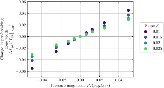
FIG. 6: The fractional change in prebreaking zone width $\Delta L_{\text{pz}}$ compared to the unforced case $\evaluated{L_{\text{pz}}}_{P=0}$ (cf. Sec. II.8) versus the nondimensional pressure magnitude $P/(\rho_{w}gL_{0}\varepsilon_{0})$. The results are shown for beach slopes $\beta=$0.010.025$$ as indicated in the legend.

We also investigate the change in the prebreaking zone width $\Delta L_{\text{pz}}$ (Sec. II.8) as a function of pressure $P/(\rho_{w}gL_{0}\varepsilon_{0})$ for four different values of the beach slope $\beta$ (Fig. 6). First, $\Delta L_{\text{pz}}$ is linearly related to the pressure magnitude, and the wind has a larger effect on $\Delta L_{\text{pz}}$ for smaller beach slopes, with $P/(\rho_{w}gL_{0}\varepsilon_{0})=-0.05$ changing the prebreaking zone width by approximately $5\text{\,}\mathrm{\char 37\relax}$ for the smallest slope $\beta=0.01$. This is because the wind has more time to affect the wave before it reaches prebreaking. This wind-induced change in prebreaking location is visible in Fig. 3, where the prebreaking location $x_{\text{pb}}$ ($\times$’s on green profiles) occurs closer to the shoreline ($+x$ direction) for offshore winds $P<0$ [Figs. 3(e) and 3(f)] than for onshore winds $P>0$ [Figs. 3(a) and 3(b)]. Additionally, we note that for the smallest slope $\beta=0.01$, the fractional change in prebreaking zone width $\Delta L_{\text{pz}}/(\evaluated{L_{\text{pz}}}_{P=0})$ is asymmetric with respect to pressure, with offshore $P/(\rho_{w}gL_{0}\varepsilon_{0})=-0.05$ yielding a $22\text{\,}\mathrm{\char 37\relax}$ larger change than onshore $P/(\rho_{w}gL_{0}\varepsilon_{0})=0.05$ (Fig. 6). For fully breaking waves, the wind-induced changes to the breaking-zone width $\Delta L_{\text{bz}}$ would likely be larger and the unforced surf zone width $\evaluated{L_{\text{bz}}}_{P=0}$ would be smaller (as waves propagate closer to shore before fully breaking), making the fractional change $\Delta L_{\text{bz}}/(\evaluated{L_{\text{bz}}}_{P=0})$ much larger.

III.3 Normalized prebreaking wave shape changes induced by wind and shoaling

((a))

((b))

((c))

FIG. 7: Prebreaking wave profile $\eta/\max_{x}(\eta)$ normalized by the maximum height versus nondimensional position $(x-x_{\text{pb}})/h_{0}$ relative to the prebreaking location $x_{\text{pb}}$. All profiles occur at prebreaking $t_{\text{pb}}$ when $\max_{x}(\operatorname{Fr})=\operatorname{Fr}_{\text{pb}}=1/3$ (cf. Sec. II.6) and display different values of the LABEL:sub@fig:wave_shapes:a pressure magnitude $P/(\rho_{w}gL_{0}\varepsilon_{0})$ and the LABEL:sub@fig:wave_shapes:b,LABEL:sub@fig:wave_shapes:c bottom slope $\beta$, as indicated in the legend. Results are shown for $\varepsilon_{0}=0.2$, $\mu_{0}=0.15$, and LABEL:sub@fig:wave_shapes:a slope $\beta=0.015$, LABEL:sub@fig:wave_shapes:b onshore $P/(\rho_{w}gL_{0}\varepsilon_{0})=0.05$, or LABEL:sub@fig:wave_shapes:c offshore $P/(\rho_{w}gL_{0}\varepsilon_{0})=-0.05$ pressure magnitude. The light gray line shows where the FWHM is measured.

As Fig. 5 quantified the shape statistics at prebreaking for all $x$, we now directly investigate the effect of pressure $P$ and shoaling $\beta$ on prebreaking wave shape by normalizing each prebreaking wave profile $\eta$ by its maximum height $\max_{x}(\eta)$ and aligning the prebreaking locations $x_{\text{pb}}/h_{0}$ (Fig. 7). Each solution is dominated by the $\sech^{2}$ wave centered near $x-x_{\text{pb}}=0$, which becomes taller and narrower as the wave shoals as required by energy conservation [45]. Furthermore, while the $\sech^{2}$ component is symmetric in time at a fixed location, it becomes slightly deformed when viewed at a fixed time as the front face moves slower than the rear face [46, 61]. We also observe a shelf behind the wave, which Miles [45] calculated by requiring that the right-moving mass-flux be conserved as the $\sech^{2}$ narrows and sheds mass. While long-duration calculations of the Miles shelf reveal a nearly horizontal shelf extending far behind the wave [62, 61], our shelf instead slopes gently downward, likely due to insufficient development time and distance.

In Fig. 7, we plot the prebreaking wave shape for fixed bottom slope $\beta$ [Fig. 7(a)] and fixed pressure magnitude $P$ [Figs. 7(b) and 7(c)]. For a fixed slope [Fig. 7(a)], the front wave faces at prebreaking are qualitatively very similar and match an unforced solitary wave of the same height. However, wind strongly affects the rear shelves as observed in Fig. 3. The offshore winds (blue) cause the shelf to be thicker and extend higher up the rear wave face than the offshore wind (reds) do, although the shelf intersects $z=0$ at $(x-x_{\text{pb}})/h_{0}\approx-10$ for all wind speeds. Nevertheless, all of the changes in Fig. 7 would likely be enhanced for fully breaking waves as wind and shoaling effects have longer to act on the wave.

We also consider the wave shape at breaking for different values of the beach slope $\beta$ with a fixed onshore [Fig. 7(b)] or offshore [Fig. 7(c)] wind. The rear half of the wave shows that bottom slope $\beta$ affects the rear shelf differently than pressure $P/(\rho_{w}gL_{0}\varepsilon_{0})$ does. While the shelf intersected $z=0$ at the same location for all wind speeds [Fig. 7(a)], increasing $\beta$ causes the intersection point (i.e., the base of the shelf) to move forward and closer to the peak. Finally, the offshore wind [Fig. 7(c)] causes a noticeably larger shelf than the onshore wind [Fig. 7(b)] for the weakest slope $\beta=0.01$ (purple), with a similar pattern observed in Fig. 4(a) ($\beta=0.015$) compared to Fig. 4(b) ($\beta=0.025$). However, this difference is much smaller for the steeper (green) slopes, implying that stronger shoaling partially suppresses the wind-induced shape change because there is less time for pressure to act prior to prebreaking.

IV Discussion

IV.1 Wind speed

Our derivation in Sec. II coupled wind to the wave’s motion through the use of a surface pressure Eq. 5. The resulting vKdV–Burgers equation 29 has a wind-induced term dependent on the pressure magnitude constant $P/(\rho_{w}gL_{0}\varepsilon_{0})$. We analyze the evolution and prebreaking of solitary waves for variable $P$ (Sec. III). While the usage of $P$ was the most natural since it is the physical coupling between wind and waves (in the absence of viscous tangential stress), measuring the surface pressure is challenging in field observations or laboratory experiments [9, 7]. Therefore, we also consider the evolution and prebreaking of the shoaling solitary waves as a function of the wind speed $U$. Zdyrski and Feddersen [25] considered a surface pressure acting on a flat-bottom KdV solitary wave initial condition [equivalent to our Eq. 30] with dimensional form

$$\eta=\varepsilon h\sech^{2}\pqty{\sqrt{\frac{3\varepsilon}{4}}\frac{x}{h}}^{2}\,,$$ (39)

with nondimensional height $\varepsilon=H/h$ and width $L=2h/\sqrt{3\varepsilon}$ in water of depth $h$. Zdyrski and Feddersen [25] then related wind speed $U$ to the surface pressure magnitude using

$$\frac{U}{\sqrt{gh}}=1\pm\sqrt{\frac{1}{5}\absolutevalue{\frac{P}{\rho_{w}gh\varepsilon}}\frac{\rho_{w}}{\rho_{a}}\frac{2}{4.91}}=1\pm\sqrt{\frac{1}{5}\absolutevalue{\frac{P}{\rho_{w}gL\varepsilon}}\frac{\rho_{w}}{\rho_{a}}\frac{4}{4.91\sqrt{3\varepsilon}}}\,,$$ (40)

where $U$ is measured at a height of half the solitary wave’s width. This parametrization originated from observations by Donelan et al. [9] of nonseparated wind forcing for periodic, shallow-water waves and was adapted to solitary waves in shallow water by Zdyrski and Feddersen [25]. The relationship is accurate for the wind and wave conditions of Donelan et al. [9], but should be interpreted qualitatively here. Note that the radicand differs by a factor of $2$ from Zdyrski and Feddersen [25] owing to the different definitions of $\varepsilon$. Even though Eq. 40 was originally applied to flat-bottomed KdV solitary waves 30, our assumption that $\gamma=L/L_{b}\ll 1$ implies that the bathymetry is approximately flat over the wave’s width $2L$. Therefore, we use Eq. 40 to translate between the pressure $P/(\rho_{w}gL_{0}\varepsilon_{0})$ and the wind speed $U$ at any point on the sloping bathymetry by using the local $\varepsilon$ and $h$ and relating the initial pressure to the local pressure $P/(\rho_{w}gL\varepsilon)=(\varepsilon_{0}L_{0}/\varepsilon L)P/(\rho_{w}gL_{0}\varepsilon_{0})$.

TABLE 2: Wind speeds as functions of pressure $P/(\rho_{w}gL\varepsilon)$ and local depth $h$ for solitary waves 39 with $\varepsilon=0.2$. $U_{\text{onshore}}$ corresponds to $P>0$ and $U_{\text{offshore}}$ to $P<0$. The conversion from $P/(\rho_{w}gL\varepsilon)$ to $U$ is given in Eq. 40.

$\absolutevalue{P/(\rho_{w}gL\varepsilon)}$	$h[$\mathrm{m}$]$	$U_{\text{onshore}}[$\mathrm{m}\text{\,}{\mathrm{s}}^{-1}$]$	$U_{\text{offshore}}[$\mathrm{m}\text{\,}{\mathrm{s}}^{-1}$]$	$h[$\mathrm{m}$]$	$U_{\text{onshore}}[$\mathrm{m}\text{\,}{\mathrm{s}}^{-1}$]$	$U_{\text{offshore}}[$\mathrm{m}\text{\,}{\mathrm{s}}^{-1}$]$
$0$	$2.5$	$4.949\,747\,468\,305\,832\,615$	$4.949\,747\,468\,305\,832\,615$	$1$	$3.130\,495\,168\,499\,705\,544$	$3.130\,495\,168\,499\,705\,544$
$0.006\,25$	$2.5$	$10.306\,434\,965\,119\,624\,654$	$-0.406\,940\,028\,507\,959\,424$	$1$	$6.518\,361\,809\,235\,211\,79$	$-0.257\,371\,472\,235\,800\,702$
$0.0125$	$2.5$	$12.525\,247\,575\,694\,282\,704$	$-2.625\,752\,639\,082\,617\,474$	$1$	$7.921\,662\,119\,339\,236\,412$	$-1.660\,671\,782\,339\,825\,324$
$0.025$	$2.5$	$15.663\,122\,461\,933\,416\,729$	$-5.763\,627\,525\,321\,751\,499$	$1$	$9.906\,228\,449\,970\,718\,059$	$-3.645\,238\,112\,971\,306\,971$
$0.05$	$2.5$	$20.100\,747\,683\,082\,732\,799$	$-10.201\,252\,746\,471\,067\,569$	$1$	$12.712\,829\,070\,178\,767\,283$	$-6.451\,838\,733\,179\,356\,195$

Table 2 shows the onshore ($P>0$) and offshore ($P<0$) wind speeds corresponding to the pressures used in our simulations for two representative depths $h$. It shows that the pressure magnitudes in our simulations correspond to physically reasonable wind speeds, with onshore $U$ from $3.1\text{\,}\mathrm{m}\text{\,}{\mathrm{s}}^{-1}13\text{\,}\mathrm{m}\text{\,}{\mathrm{s}}^{-1}$ for water $1\text{\,}\mathrm{m}$ deep or $4.9\text{\,}\mathrm{m}\text{\,}{\mathrm{s}}^{-1}20\text{\,}\mathrm{m}\text{\,}{\mathrm{s}}^{-1}$ for water $2.5\text{\,}\mathrm{m}$ deep. Notice that unforced waves with $P=0$ correspond to a wind speed matching the wave phase speed $U=c$, with $c$ approximately the linear shallow-water phase speed $c\approx\sqrt{gh}$. In particular, this means that onshore $P>0$ and offshore $P<0$ winds with the same pressure magnitude $\absolutevalue{P}$ will have different wind-speed magnitudes $\absolutevalue{U}$. Additionally, note that keeping $P$ fixed implies that the wind speed $U$ changes as the wave shoals. This is mostly due to the decrease in the phase speed $c\propto\sqrt{gh}$, with higher-order effects coming from the $\varepsilon$ and $L$ dependence of the radicand in Eq. 40. Finally, note that as the wave shoals and $\varepsilon$ increases, the height at which the wind speed is measured $z=L/2=h/\sqrt{3\varepsilon}$ decreases.

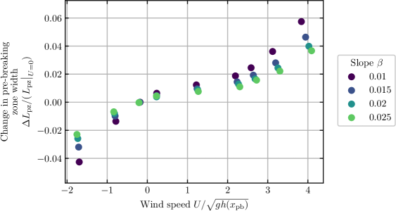
FIG. 8: The fractional change in prebreaking zone width $\Delta L_{\text{pz}}$ compared to the unforced case $\evaluated{L_{\text{pz}}}_{U=0}$ (cf. Sec. II.8) versus the nondimensional wind speed $U/\sqrt{gh(x_{\text{pb}})}$ normalized by the local, shallow-water phase speed $\sqrt{gh(x_{\text{pb}})}$ and evaluated at a height of half the solitary wave width $L$. The results are shown for beach slopes $\beta=$0.010.025$$.

We now reexamine our results regarding the prebreaking zone width (Fig. 6) in terms of the wind speed $U/\sqrt{gh(x)}$ using Eq. 40. In addition to changing the abscissa of the plot (Fig. 8), we also modify the definition of the change in the prebreaking zone width $\Delta L_{\text{pz}}\coloneqq L_{\text{pz}}-\evaluated{L_{\text{pz}}}_{U=0}$ by comparing and normalizing each prebreaking zone width to the $U=0$ case rather than the $P=0$ case. This transformation changes the initially straight lines of Fig. 6 into approximate pairs of upward- and downward-facing $\sqrt{\Delta L_{\text{pz}}}$ curves shifted to the right by one unit (Fig. 8). Furthermore, we see that $\Delta L_{\text{pz}}$ is now much flatter for onshore winds ($U>0$) than for equal magnitude offshore winds ($U<0$). This is due to the inflection point of the unforced case ($P=0$) being shifted to the right at $U/\sqrt{gh}=1$.

IV.2 Isolating the effect of wind

For no wind ($P=0$), solitary wave shoaling is well understood to generate a rear shelf [45]. The variation in the rear shelf’s thickness with $P$ (Fig. 7) is reminiscent of the variability in the wind-generated bound, dispersive, and decaying tails of flat-bottom solitary waves [25]. Additionally, Zdyrski and Feddersen [25] showed that flat-bottom, wind-generated tails are analogous to the dispersive tails of KdV solutions with non-solitary-wave initial conditions [53]. Both the rear shelf and wind-generated tail can be viewed as weak perturbations to the KdV equation by transforming the nondimensional vKdV–Burgers equation 28 into a constant-coefficient, perturbed KdV equation by defining $\nu\coloneqq(3/2)(\varepsilon_{0}/\mu_{0})\eta_{0}/\tilde{h}^{2}$ and $\tau\coloneqq\int\tilde{c}dx_{1}\mu_{0}/(6\gamma_{0})$:

$$\partialderivative{\nu}{\tau}+6\nu\partialderivative{\nu}{\xi_{+}}+\partialderivative[3]{\nu}{\xi_{+}}=-\frac{9}{4}\frac{1}{\tilde{h}}\partialderivative{\tilde{h}}{\tau}\nu-3\frac{P_{0}}{\mu_{0}}\frac{1}{\tilde{c}^{3}}\partialderivative[2]{\nu}{\xi_{+}}\,.$$ (41)

The first term on the right-hand-side (RHS) is the shoaling term which leads to the rear shelf [45], and the second term is the wind-induced Burgers term [25]. Our derivation assumed all terms in Eq. 41 were the same order, and indeed $\partial_{\tau}\tilde{h}/\tilde{h}\sim 6\gamma_{0}/\mu_{0}=$1.02.6$$ is order one. However, the forcing term $\absolutevalue{P_{0}}/\mu_{0}=(4/3)\absolutevalue{P_{0}}/\varepsilon_{0}=$00.07$$ is much smaller than unity and is a weak perturbation to the sloping-bottom KdV equation with its $\sech^{2}$ solitary-wave and shelf solution.

Perturbed KdV equations similar to Eq. 41 received some attention in past literature. In particular, the unforced, shoaling case can be recast in a number of asymptotically equivalent forms including Eqs. 28 or 41 with $P=0$. Previous authors applied different mathematical techniques to these various asymptotic forms to derive closed-form approximate solutions. For instance, Knickerbocker and Newell [61] solved the unforced analog of Eq. 28 using conservation laws. Alternatively, Grimshaw [63] used a multiple-scale analysis to solve a windless, modified form of Eq. 28. Similarly, Ablowitz and Segur [64] solved the $P=0$ version of Eq. 41 using a direct perturbation solution while Newell [46] solved it using the inverse scattering transform. Since Eq. 41 shows that shoaling and wind forcing can be treated on an equal footing, it should be possible to extend these analyses to wind-forced solitary waves. However, such an analysis is outside the scope of the current work, but is suitable for future work.

((a))

((b))

((c))

((d))

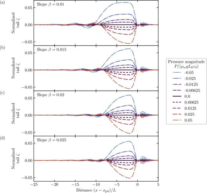
FIG. 9: Normalized tail $\zeta$ Eq. 42 versus nondimensional position $(x-x_{\text{pb}})/L$ relative to the prebreaking location $x_{\text{pb}}$. The wave profile is normalized by the maximum height $\max_{x}(\eta)$, and the spatial coordinate $(x-x_{\text{pb}})$ is normalized by the wave width $L$ [Eq. 43]. All profiles occur at prebreaking $\max_{x}(\operatorname{Fr})=\operatorname{Fr}_{\text{pb}}=1/3$ (cf. Sec. II.6) and are displayed for bottom slopes $\beta$ of LABEL:sub@fig:wave_shape_differences:a $0.01$, LABEL:sub@fig:wave_shape_differences:b $0.015$, LABEL:sub@fig:wave_shape_differences:c $0.02$, and LABEL:sub@fig:wave_shape_differences:d $0.025$. Results are shown for $\varepsilon_{0}=0.2$, $\mu_{0}=0.15$, and pressure magnitude $\absolutevalue{P/(\rho_{w}gL_{0}\varepsilon_{0})}$ up to $0.05$, as indicated in the legend. The solid black line is the unforced case $P=0$ and is zero by definition.

Reverting back to dimensional variables, we isolate the effect of wind by separating out the $\sech^{2}$ solitary wave and the Miles rear shelf using the unforced $P=0$ normalized profiles to represent shoaling and rear-shelf generation. We define a normalized tail $\zeta$ as the difference between the forced and unforced $P=0$ normalized profiles of Fig. 7:

$$\zeta\coloneqq\frac{\eta}{\max_{x}(\eta)}-\evaluated{\pqty{\frac{\eta}{\max_{x}(\eta)}}}_{P=0}\,.$$ (42)

For constant depth, the height $H$ and width $L$ of unforced, $\sech^{2}$ solitary waves always satisfy $HL^{2}=\text{const}$. Since our numerical results (e.g., Fig. 7) are dominated by the $\sech^{2}$ solitary wave profile, scaling the wave profile by $H$ requires that we scale the spatial coordinate by $L\propto 1/\sqrt{H}$ to respect this symmetry and enable comparison of waves with different heights. We replace $h\to h(x_{\text{peak}})$ in the expression for the flat-bottom solitary wave width $L$ Eq. 39 to yield the wave width for a slowly varying depth as

$$L=h(x_{\text{peak}})\sqrt{\frac{4h(x_{\text{peak}})}{3H}}\,.$$ (43)

We normalize the spatial coordinate as $x/L$ to compare the normalized tails $\zeta$ in Fig. 9.

We show the normalized tail $\zeta$ versus $(x-x_{\text{pb}})/L$ for different pressures $P$ and bottom slopes $\beta$ in Fig. 9. First, increasing the pressure magnitude $\absolutevalue{P}$ increases the tail’s amplitude and wavelength. For example, the wavelength with $\beta=0.01$ is approximately $5L$ for $P/(\rho_{w}gL_{0}\varepsilon_{0})=-0.025$ and $7.5L$ for $P/(\rho_{w}gL_{0}\varepsilon_{0})=-0.05$. This amplitude increase is expected, as higher pressures put more energy into the tail, causing growth. Additionally, increasing the bottom slope $\beta$ decreases the shelf’s width and the tail’s amplitude without noticeably changing its wavelength. We can explain the narrower shelf and smaller amplitude by recognizing that larger $\beta$’s cause the wave to reach prebreaking (when these profiles are compared) earlier, decreasing the time over which the wind (tail) and shoaling (shelf) act. The wavelength’s independence of the beach slope $\beta$ also implies that the width $L$ of the solitary wave sets the tail’s wavelength. Additionally, we note that onshore ($P>0$) and offshore ($P<0$) winds change the polarity of the tail, consistent with Zdyrski and Feddersen [25]. Lastly, wind induces a small, bound wave in front of the prebreaking solitary wave with minimum near $(x-x_{\text{pb}})=0$ and extremum near $(x-x_{\text{pb}})/L\approx 2$ of the same polarity as the rear shelf (Fig. 9), similar to the flat-bottom results of Zdyrski and Feddersen [25].

Hence, the numerically calculated wave profiles (Fig. 7) are a superposition of the $\sech^{2}$ solitary wave, Miles’ shelf [45], and a wind-induced bound, dispersive, and decaying tail [25]. Furthermore, this decomposition of the full wave enables us to understand the effects of wind and shoaling from previous studies. The $\sech^{2}$ solitary wave grows and narrows due to wave shoaling [45] and wind forcing [25]. Miles’ shelf is generated by the mass flux of the growing wave. The shelf’s absence from the normalized tails in Fig. 9 implies its shape is largely unchanged by the wind, and its amplitude for a given bottom slope $\beta$ is approximately proportional to the $\sech^{2}$ solitary wave. Finally, the amplitude and wavelength of the bound, dispersive, and decaying tail grow with the $\sech^{2}$ solitary wave [25].

This decomposition relies on the assumption that the tail and shelf are both small compared to the solitary wave and do not influence each other or the solitary wave. This is only possible when the wind-forcing $P_{0}$ is weak and the wave width-to-beach width ratio $\gamma_{0}$ is small. Miles [45] analyzed a vKdV equation requiring the same weak-slope assumption $\gamma_{0}\sim\varepsilon_{0}$, though his adiabatic results required an even smaller $\gamma_{0}=\order{${10}^{-2}$}$ [31]. The realistic beach widths we utilized yield a $\gamma_{0}=$3\text{\times}{10}^{-2}6\text{\times}{10}^{-2}$$ somewhat larger than this adiabatic regime, and the $\gamma_{0}/\varepsilon_{0}$ term in Eq. 41 is not as small as the pressure-forcing term, implying some nonlinear interactions between the shoaling-induced shelf and the $\sech^{2}$ solitary are possible. For this reason, we subtracted off the unforced solitary wave and shelf rather than approximate them analytically. Nevertheless, the pressure forcing $\absolutevalue{P_{0}}/\mu_{0}=$00.07$$ we used was sufficiently small that the weak wind forcing can be considered to interact linearly, as seen in the clean separation between pressure-induced tail and $\sech^{2}$ plus shelf in Fig. 9. Thus, we show that there are physically reasonable parameter regimes wherein wave shape and evolution are the superpositions of the previously understood shoaling- and wind-induced effects.

IV.3 Breakpoint location comparison to prior laboratory experiments and models

Numerical studies investigated the effect of wind on the breaking of shoaling solitary [40] and periodic [41] waves using a RANS $k$–$\varepsilon$ model to simulate both the air and water. Xie [40] considered solitary waves with initial height $H_{0}/h_{0}=0.28$ on a beach slope of $0.05$ with onshore winds of up to $U/\sqrt{gh_{0}}=3$, while Xie [41] investigated periodic waves with initial height $H_{0}/h_{0}=0.3$ and initial inverse wavelength $h_{0}/\lambda_{0}=0.1$ on a beach slope of $0.03$ forced by onshore winds up to $U/\sqrt{gh_{0}}=2$. These studies determined that the (absolute) maximum wave heights $\max_{t}(\eta)/h_{0}$ increased with increasing onshore wind at each location $x<x_{\text{b}}$ prior to breaking at $x_{\text{b}}$, consistent with our findings in Fig. 5(b). Furthermore, Xie [40] found the effect of wind on breaker depth is significant while the effect on breaker height is minor, again consistent with our prebreaking findings. Finally, comparing wave profiles in Xie [40] shows that onshore winds increase the wave slope at a fixed location, which is consistent with our Fig. 5(c).

For periodic waves, previous laboratory experiments also investigated wind’s effect on the breaking characteristics of shoaling waves [38, 39]. Douglass [38] considered waves with initial height $H_{0}/h_{0}=0.3$ and initial inverse wavelength $h_{0}/\lambda_{0}=0.1$ under wind speeds of up to $U/\sqrt{gh_{0}}=\pm 2.3$ on a beach with slope $0.04$ while King and Baker [39] considered waves with initial height $H_{0}/h_{0}=0.2$ and initial inverse wavelength $h_{0}/\lambda_{0}=0.3$ with wind speeds of up to $U/\sqrt{gh_{0}}=\pm 1.1$ on a beach with slope $0.05$. Douglass [38] measured how wind speed affects wave parameters and changes the surf zone width for periodic waves. Directly comparing our Fig. 8 to Fig. 2 of Douglass [38], we see many qualitative similarities, including the prebreaking zone width’s flatter response near $U=0$ and a stronger response for offshore winds ($U<0$) than the corresponding onshore winds ($U>0$), with our change roughly four times smaller than theirs. Furthermore, the laboratory studies also found that the relative breaking height $H_{\text{b}}/h_{\text{b}}$, normalized by the breaking depth, decreased by as much as $40\text{\,}\mathrm{\char 37\relax}$ for offshore wind speeds of $U/\sqrt{gh_{\text{b}}}=4$ and increased by up to $10\text{\,}\mathrm{\char 37\relax}$ for onshore wind speeds of $U/\sqrt{gh_{\text{b}}}=-2$ compared to the unforced case [38, 39]. By comparison, over those same wind speed ranges of $U/\sqrt{gx_{\text{pb}}}=1\pm 3$, our simulations found that the relative prebreaking height $h_{\text{pb}}/x_{\text{pb}}$ varied by approximately $1\text{\,}\mathrm{\char 37\relax}$ between onshore and offshore winds [Fig. 5(b)], with the same polarity as the laboratory experiments. Finally, Douglass [38] observed only a slight dependence of the breaking wave height on wind speed, which is consistent with our finding that offshore-forced waves are only $1\text{\,}\mathrm{\char 37\relax}$ larger than onshore-forced waves at prebreaking. On the contrary, King and Baker [39] measured no statistically significant change with wind speed in the ratio between the change in the fractional change $(H_{\text{b}}-\evaluated{H_{\text{b}}}_{U=0})/\evaluated{H_{\text{b}}}_{U=0}$ of (absolute) breaking height $H_{b}$ compared to the unforced case $\evaluated{H_{\text{b}}}_{U=0}$. This is surprising, as both our results and those of Douglass [38] had near-constant relative (pre)breaking height $\Delta(H_{\text{b}}/h_{\text{b}})$. Indeed, constant $\Delta(H_{\text{b}}/h_{\text{b}})$ implies $\Delta H_{\text{b}}/\evaluated{H_{\text{b}}}_{U=0}$ must vary with wind (we find approximately $\pm$5\text{\,}\mathrm{\char 37\relax}$$ at prebreaking) to counteract the varying of $\Delta h_{\text{b}}/\evaluated{h_{\text{b}}}_{U=0}=\Delta L_{b}/\evaluated{L_{b}}_{U=0}$ with wind that Douglass [38], King and Baker [39], and we all find.

Our results qualitatively agree with prior numerical results on solitary waves [40] as well as experimental and numerical results on periodic waves [38, 39, 41], and the quantitative mismatch can be partly explained by the different nondimensional parameters. All three studies mentioned used larger initial waves ($\varepsilon_{0}\approx 0.3$), so nonlinear effects were likely more important. They also used steeper beach slopes, enhancing the shoaling effect. Additionally, while the surf zone width change is roughly four times larger for Douglass [38] than for our simulations over the same wind-speed range, Douglass [38] investigated waves that were actually breaking. In contrast, we stopped our simulations at prebreaking $\max_{x}(\operatorname{Fr})=\operatorname{Fr}_{\text{pb}}=1/3$, significantly before actual breaking $\max_{x}(\operatorname{Fr})\approx 1$ [33], thus we expect smaller changes to the fractional surf prebreaking zone width (cf. Sec. III.2).

IV.4 Wave shape comparison to prior laboratory experiments

((a))

((b))

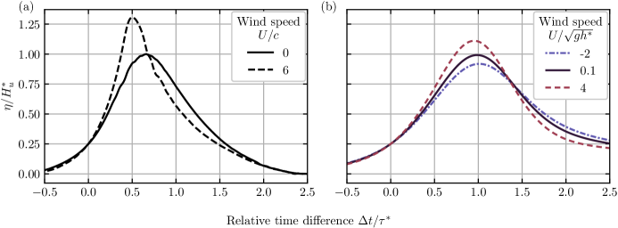
FIG. 10: Nondimensional wave profile $\eta/H^{*}_{u}$ at a fixed location versus nondimensional time $\Delta t/\tau^{*}$ with $\eta$ normalized by the no-wind wave height $H^{*}_{u}$. The time difference $\Delta t\coloneqq t-t_{0.25}$ is relative to the time when the profile reaches $\eta/H^{*}_{u}=0.25$ and is normalized by the unforced solitary wave temporal width $\tau^{*}=L^{*}_{u}/\sqrt{gh^{*}}$ at a depth $h^{*}$, with $L^{*}_{u}$ the unforced spatial width [Eq. 43]. LABEL:sub@fig:fv2005_comparison:a Periodic wave laboratory results from Feddersen and Veron [23] with $\varepsilon_{0}\approx 0.28$, $\mu_{0}=0.035$, and $\beta=0.125$. The solid line represents the no-wind case $U/c=0$ and the dashed line corresponds to an onshore wind $U/c=6$, as indicated in the legend. The waves began shoaling at a depth of $h_{0}=$0.37\text{\,}\mathrm{m}$$ and were measured at a nondimensional depth $h^{*}/h_{0}=0.62$. The wave height $\eta$ is plotted relative to the wave trough $\min_{t}(\eta)$. LABEL:sub@fig:fv2005_comparison:b Numerical results for $\varepsilon_{0}=0.2$, $\mu_{0}=0.15$, and $\beta=0.015$ at a nondimensional water depth $h^{*}/h_{0}=0.69$ and for nondimensional wind speeds $U/\sqrt{gh^{*}}$ [cf. Eq. 40] as indicated in the legend.

Feddersen and Veron [23] experimentally examined the effect of wind on the temporal shape of shoaling, periodic waves at a fixed location for no-wind ($U/c=0$) and onshore-wind ($U/c=6$) cases [cf. Fig. 10(a)]. The waves began shoaling at a depth of $h_{0}=$0.37\text{\,}\mathrm{m}$$ and were observed at a depth $h^{*}/h_{0}=0.62$. To enable direct comparison with our results, we normalized the profile by the height of the no-wind profile $H^{*}_{u}$ at depth $h^{*}$. We also normalized the time coordinate with an unforced solitary wave’s temporal width $\tau^{*}=L^{*}_{u}/\sqrt{gh^{*}}$ at depth $h^{*}$, where the unforced spatial width $L^{*}_{u}$ is related to the wave height via an equation similar to Eq. 43. We observe that the onshore wind increases the wave height and causes earlier peak arrival, relative to the arrival time of $\eta/H^{*}_{u}=0.25$ (Fig. 10). For comparison, our numerical results [Fig. 10(b)] over different wind speeds, calculated using Eq. 40, are shown at $x/h=20.1$ corresponding to $h^{*}/h_{0}=0.68$. This corresponds to $x_{\text{pb}}$ for the strongest onshore wind $U/\sqrt{gh^{*}}=4$ (i.e., $P=0.05$) case. We truncated the time series at $\operatorname{Fr}=1/2$, instead of $\operatorname{Fr}_{\text{pb}}=1/3$, to enable qualitative comparison of the strong-wind numerical case ($U/\sqrt{gh^{*}}=4$) with the laboratory onshore-wind case ($U/c=6$). However, we note that this result is strictly out of the asymptotic range.

Our numerical results [Fig. 10(b)] are qualitatively similar to the experimental results of Feddersen and Veron [23] [Fig. 10(a)], despite different experimental and model conditions. Specifically, Feddersen and Veron [23] presented shallower ($h^{*}/h_{0}=0.62$) measurements of shoaling periodic waves ($h_{0}/\lambda_{0}=0.27$) forced by stronger laboratory winds ($U/c=6$) in contrast to our deeper ($h^{*}/h_{0}=0.68$) simulations of solitary waves ($h_{0}/\lambda_{0}\to 0$) for weaker winds ($U/\sqrt{gh^{*}}=4$). Therefore, we display the results side by side as opposed to overlaid to emphasize the qualitative comparison. Onshore wind causes wave growth and narrowing for both laboratory observations and numerical results. The peaks of the onshore-forced waves occur earlier (relative to the time of $\eta/H^{*}_{u}=0.25$) due to wave narrowing, as seen in Fig. 5(d). Finally, the rear faces of the onshore-forced waves ($\Delta t/\tau^{*}$ from $12.5$) dip below the no-wind cases. Numerical results with offshore wind continue the pattern. The qualitative similarities between our results and that of Feddersen and Veron [23] suggests that the our vKdV–Burgers equation captures the essential aspects of wind-induced effects on shoaling wave shape. No other theoretical model has yet shown such qualitative similarity with wind-forced wave shape experiments, despite the differences (e.g., periodic versus solitary) between the laboratory and numerical studies.

V Conclusion

While shoaling-induced changes to wave shape are well understood, the interaction of wind-induced and shoaling-induced shape changes has been less studied and lacked a theoretical framework. Utilizing a Jeffreys-type wind-induced surface pressure, we defined four nondimensional parameters that controlled our system: the initial wave height $\varepsilon_{0}$, the inverse wavelength squared $\mu_{0}$, the pressure strength $P_{0}$, and the wave width-to-beach width ratio $\gamma_{0}$. We leveraged these small parameters to reduce the forced, variable-bathymetry Boussinesq equations to a variable-coefficient Korteweg–de Vries–Burgers equation for the wave profile $\eta$. We also extended the convective breaking criterion of Brun and Kalisch [35] to include pressure and shoaling. A third-order Runge-Kutta solver determined the time evolution of a solitary wave initial condition up a planar beach under the influence of onshore and offshore winds. Stopping the simulations at a prebreaking Froude number of $1/3$ revealed that the prebreaking relative height and maximum slope are largely independent of wind speed, but onshore winds cause a narrowing of the waves. The width of the prebreaking zone is strongly modulated by wind speed, with offshore wind decreasing the prebreaking zone width by approximately $5\text{\,}\mathrm{\char 37\relax}$ for the mildest beach slopes. Investigating the wave shape at prebreaking revealed that the front of the wave is relatively unchanged and matches an unforced solitary wave, while the rear shelf is strongly affected by wind speed and bottom slope. We isolated the effect of wind from the effect of shoaling and revealed a bound, dispersive, and decaying tail similar to wind-induced tails on flat bottoms. By leveraging the relationship between surface pressure $P$ and wind speed $U$, we directly compared our results to existing experimental and numerical results. We found qualitative agreement in surf width changes and wave height changes and expect better quantitative agreement as the waves propagate closer to breaking. These results suggest that wind significantly impacts wave breaking, and our simplified model highlights the relevant physics and changes to wave shape. Future avenues of research could include calculating asymptotic, closed form solutions to Eq. 41 or deriving coupled equations for both the water and air motions to more accurately predict the surface pressure distribution.