Radio and X-ray observations of the luminous Fast Blue Optical Transient AT 2020xnd

Abstract

We present deep X-ray and radio observations of the Fast Blue Optical Transient (FBOT) AT 2020xnd/ZTF20acigmel at $z=0.2433$ from $13$ d to $269$ d after explosion. AT 2020xnd belongs to the category of optically luminous FBOTs with similarities to the archetypal event AT 2018cow. AT 2020xnd shows luminous radio emission reaching $L_{\nu}\approx 8\times 10^{29}$ erg s^-1Hz^-1 at 20GHz and $75$d post explosion, accompanied by luminous and rapidly fading soft X-ray emission peaking at $L_{X}\approx 6\times 10^{42}$ erg s^-1. Interpreting the radio emission in the context of synchrotron radiation from the explosion’s shock interaction with the environment we find that AT 2020xnd launched a high-velocity outflow ($v\sim$0.1–0.2$c$) propagating into a dense circumstellar medium (effective $\dot{M}\approx 10^{-3}\rm{M_{\odot}}$ yr^-1 for an assumed wind velocity of $v_{w}=1000\,$km s^-1). Similar to AT 2018cow, the detected X-ray emission is in excess compared to the extrapolated synchrotron spectrum and constitutes a different emission component, possibly powered by accretion onto a newly formed black hole or neutron star. These properties make AT 2020xnd a high-redshift analog to AT 2018cow, and establish AT 2020xnd as the fourth member of the class of optically-luminous FBOTs with luminous multi-wavelength counterparts.

1 Introduction

The advent of wide-field and high-cadence optical transient surveys, along with real-time discovery efforts, has expanded the parameter space in the search for new classes of extragalactic transient with rapid evolution timescales. Observations from such surveys have revealed a variety of optical transients spending $\lesssim 10$ days above half maximum brightness, atypical for the majority of extragalactic transients previously discovered (e.g., Kasliwal et al. 2010; Poznanski et al. 2010). Among these are the Fast Blue Optical Transients (FBOTs), characterized by their rapid rise to maximum light ($\lesssim 10\,\rm{d}$), peak optical luminosity reaching $L_{pk}>10^{43}\,\rm{erg}\,s^{-1}$, and persistently blue colors (e.g. Drout et al. 2014; Arcavi et al. 2016; Tanaka et al. 2016; Pursiainen et al. 2018; Rest et al. 2018; Ho et al. 2021; Perley et al. 2020). FBOTs appear to be intrinsically rare events, occurring at between 1% and 10% of the core collapse supernova rate in the local Universe (Drout et al., 2014; Pursiainen et al., 2018; Tampo et al., 2020; Li et al., 2011).

The most optically luminous FBOTs are further distinguished from other rapidly evolving extragalactic transients - such as subluminous Type IIb/Ib SNe (Poznanski et al., 2010; Ho et al., 2021); luminous Type Ibn or hybrid IIn/Ibn SNe (Ho et al., 2021); Type IIn SNe (e.g. Ofek et al. 2010) - based on the presence of highly luminous X-ray and radio emission, comparable to those seen in short gamma-ray bursts and well in excess of what is seen in typical core-collapse SNe (e.g. Margutti et al. 2019; Coppejans et al. 2020; Ho et al. 2019a, 2020a; Bright et al. 2020a; Matthews et al. 2020, and see Figure 1). Although the population of FBOTs with associated high energy emission remains small, FBOTs with luminous radio and X-ray emission are rarer still, occurring at $\lesssim 1\%$ of the core-collape supernovae (CCSNe) rate below $z\sim 0.5$ (Coppejans et al., 2020; Ho et al., 2021). In the optical, FBOTs do not show a ${}^{56}\rm{Ni}$ powered decay tail, do show high temperature photospheric emission, and are preferentially located in dwarf galaxies (Coppejans et al., 2020; Perley et al., 2021).

The prototypical optically luminous FBOT with associated emission at X-ray and radio wavelengths is AT2018cow (Prentice et al. 2018) which, at only $\sim 60\,\rm{Mpc}$, was the subject of extended observing campaigns at cm, mm, and X-ray wavelengths (Margutti et al., 2019; Ho et al., 2019b; Kuin et al., 2019; Perley et al., 2019; Nayana & Chandra, 2021; Rivera Sandoval et al., 2018). The radio observations revealed the presence of a shock with velocity of $\sim 0.1c$ interacting with a dense and asymmetric CSM, while the X-ray emission was in excess of an extrapolation of the radio spectrum. This X-ray excess suggested an additional emission component, which was interpreted as a central engine - an accreting compact object or a spin-powered magnetar. The X-ray spectrum of AT2018cow also clearly contained multiple components, with an excess above $\sim 10\,\rm{keV}$ seen at early times that had vanished at $\sim 15\,\rm{d}$ post explosion. The origin of this hard excess remains unclear, Margutti et al. (2019) interpreted it as a Compton hump feature resulting from X-rays interacting with a fast ejecta shell, or reflection off of an accretion funnel. Both scenarios suggest an X-ray source embedded within the explosion. While X-ray observations of CSS161010 (Coppejans et al., 2020) at $d\approx 150$ Mpc were not as comprehensive as for AT2018cow, the former showed a similar excess relative to its well sampled radio SEDs, suggesting that the presence of a central engine is a feature of the FBOTs (Margutti et al., 2019; Coppejans et al., 2020).

In this work we present radio and X-ray observations of the FBOT AT 2020xnd (ZTF20acigmel), the third FBOT with both luminous X-ray and radio emission. Additional radio observations of AT2020xnd/ZTF20acigmel (including high frequency monitoring with the SMA/NOEMA) were obtained by an independent observing team and are presented in Ho et al.+2021. AT 2020xnd was discovered on 2020 October 12 by the Zwicky Transient Facility (ZTF, Bellm et al. 2019; Graham et al. 2019) as part of the two-day cadence public survey (Perley et al. 2021). Follow-up observations identified a candidate (dwarf) host galaxy at $z=0.2433$. Based on the rapid rise and decay, the blue color, the dwarf galaxy host, and the high optical luminosity of this source Perley et al. (2021) classified AT 2020xnd as an FBOT.

Upon the announcement that AT 2020xnd was producing luminous radio emission (Ho et al., 2020a), we initiated a multi-wavelength observing campaign on the target beginning at fifteen days post discovery. Our campaign included observations at radio (AMI-LA, ATCA, eMERLIN, GMRT, MeerKAT, VLA), sub-mm/mm (ALMA, GBT), and X-ray (Chandra, XMM-Newton) frequencies. We particularly highlight the use of the MUSTANG-2 bolometer camera on the GBT, which provided us with early time mm data, demonstrating its suitability for rapid transient follow-up at high frequencies.

We structure the rest of this manuscript as follows. In Section 2 we describe our observations and the data reduction process. In Section 3 we derive and present the results for our analysis of our radio and X-ray observations. Finally, in Section 4 and Section 5 we discuss our results and give our conclusions, respectively.

2 Observations

Throughout this paper, measurements in time are in reference to the explosion date ($T_{0}$), which is MJD $59132.0$ (Perley et al., 2021), and are in the observed frame, unless otherwise specified. Uncertainties are reported at the $1\sigma$ (Gaussian equivalent) confidence level (c.l.) and upper limits at the $3\,\sigma$ c.l. unless explicitly noted. We adopt standard $\Lambda$CDM cosmology with H${}_{0}=69.6$ km s^-1 Mpc^-1, $\Omega_{\rm{M}}=0.286$, $\Omega_{\rm{\Lambda}}=0.714$ (Bennett et al., 2014). At $z=0.2433$ (Perley et al., 2021) the luminosity distance of AT 2020xnd is $D_{L}=1232\,\rm{Mpc}$ and the angular diameter distance is $D_{\theta}=797\,\rm{Mpc}$.

2.1 Radio

In this section we describe our large radio campaign on AT 2020xnd. A summary of all of our radio observations are given in Table 1. The calibrators used and array configurations are given in Table 2.

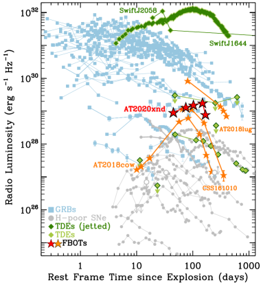
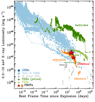
Figure 1: Left Panel: The evolving radio luminosities of extragalactic H-poor explosive transients, including long GRBs (light blue squares), SNe (light-gray circles), TDEs (green diamonds) at $\nu\approx 5$ GHz. Like the other FBOTs (orange stars), AT 2020xnd (red stars) drops off rapidly at late times. Right Panel: X-ray parameter space for the same set of transients. References: Margutti et al. (2019); Alexander et al. (2020); Coppejans et al. (2020); Ho et al. (2020b) and references therein.

2.1.1 Australia Telescope Compact Array

The field of AT 2020xnd was observed with the Australia Telescope Compact Array (ATCA) under project codes CX471 (PI Bright) and CX472 (PI Ho), beginning on 2020 October 25 ($T_{0}+15$d). Data were recorded with either the $4\,\rm{cm}$ receiver (which collects data simultaneously at 5.5 and $9\,\rm{GHz}$), the $15\,\rm{mm}$ receiver (which collects data simultaneously at 17 and $19\,\rm{GHz}$), or the $7\,\rm{mm}$ receiver (which collects data simultaneously at 33 and $35\,\rm{GHz}$). Each frequency was observed with a $2\,\rm{GHz}$ bandwidth and processed by the Compact Array Broadband Backend (CABB; Wilson et al. 2011). Data taken as part of CX471 were reduced and imaged in miriad (Sault et al., 1995) using standard techniques. Data from CX472 are reported in Dobie et al. 2020b, c, a. For observations taken with the $15\,\rm{mm}$ or $7\,\rm{mm}$ receiver the sub-bands were jointly imaged in order to double the bandwidth and increase image sensitivity.

2.1.2 Karl G. Jansky Very Large Array

We initiated Karl G. Jansky Very Large Array (VLA) observations of AT 2020xnd as part of program VLA/20A-354 (PI Margutti) beginning on 2020 November 5 (MJD 59158, $T_{0}+26$d). Observations were taken at S, C, X, Ku, K, and Ka bands, utilizing the WIDAR correlator, with a $2\,\rm{GHz}$ bandwidth at S-band, a $4\,\rm{GHz}$ bandwidth at C and X-band, a $6\,\rm{GHz}$ bandwidth at Ku-band, and a $8\,\rm{GHz}$ bandwidth at K-band and Ka-band. AT 2020xnd lies in the declination range of the Clarke satellite belt as observed from the VLA, and as such we shifted the basebands at C and X bands to reduce the impact of radio frequency interference. Data were reduced with the VLA CASA (McMullin et al. 2007) calibration pipeline version 2020.1.0.36 and then manually inspected, further flagged, and reprocessed through the pipeline. The final imaging was performed using WSClean (Offringa et al., 2014; Offringa & Smirnov, 2017) where we used -fit-spectral-pol=2 (equivalent to using two Taylor terms when using CASA) to account for the wide fractional bandwidth of the VLA. Images were created using a Briggs parameter between 0 and 1 depending on the array configuration. Where we measured the flux within small sub-bands of the bandwidth we set -no-mf-weighting in order to avoid the creation of artificial spectral structure. Fitting was performed using pybdsf (Mohan & Rafferty, 2015) with the size of the source fixed to that of the synthesized beam.

2.1.3 Enhanced Multi-Element Radio Linked Interferometer Network

We were awarded DDT observations (project ID DD10005, PI Bright) of AT 2020xnd with the Enhanced Multi-Element Radio Linked Interferometer Network (eMERLIN) and observed the field of AT 2020xnd on 2020 November 6 ($T_{0}+27$d). Observations were conducted at a central frequency of $5.075\,\rm{GHz}$ with a $512\,\rm{GHz}$ bandwidth. The Lovell telescope was not included in the array. Data calibration was performed with the eMERLIN CASA pipeline using standard techniques. We did not detect emission consistent with the position of AT 2020xnd. We triggered a further four C-band observations as part of project ID CY11008 (PI Bright). Further observations were reduced using the same strategy, with imaging performed manually on the pipeline output, and we detected the source in one epoch at $T_{0}+102$d.

2.1.4 Robert C. Byrd Green Bank Telescope

We observed AT 2020xnd with the Robert C. Byrd Green Bank Telescope (GBT) with the MUSTANG-2 instrument (Dicker et al., 2014) beginning on $T_{0}+28\,\rm{d}$ (MJD 59160). Data were taken under projects GBT20B_437 (PI Bright) and GBT20B_440 (PI Bright). MUSTANG-2 is a bolometer camera providing $9^{\prime\prime}$ arcsecond resolution and high continuum sensitivity between 75 and $105\,\rm{GHz}$. Due to the wide bandwidth that MUSTANG-2 is sensitive to, the effective central frequency of any given observation depends on the spectral index of the source being observed. The spectral index from AT 2020xnd (as determined by our modeling in §3) is between $\sim 1.5$ and $0$ through the MUSTANG-2 bandpass, which results in a central frequency between 88.6 and $88.9\,\rm{GHz}$. We therefore use $90\,\rm{GHz}$ a the central frequency, and do not consider the small shift due to spectral index. The MUSTANG-2 data is reduced via the MIDAS pipeline, which is described in Romero et al. (2020). The MIDAS pipeline relies on Fourier filtering the data and subtraction of principle components (via PCA). For point sources such as AT 2020xnd the recovered flux density is insensitive to the range of typical filtering parameters used. We used six principal components and a notched Fourier filter, keeping frequencies between 0.07 and 41 Hz. The MUSTANG-2 data were flux calibrated relative to Neptune and a nearby secondary calibrator (a point source) was used to track pointing and gain shifts during each night. The observations of the secondary calibrators were also used to determine the beam size for each night.

2.1.5 Giant Metrewave Radio Telescope

We observed the field of AT 2020xnd with the Giant Metrewave Radio Telescope (GMRT) beginning on $T_{0}+162$d at $0.75$GHz and $1.25$GHz, under program 39_034 (PI Matthews). The data were reduced manually using standard calibration techniques, with multiple rounds of phase-only and then amplitude and phase self-calibration performed. We then performed a single round of direction-dependent self-calibration using killMS (Tasse, 2014; Smirnov & Tasse, 2015) to solve for direction dependent gains and DDFacet (Tasse et al., 2018) to perform imaging and create a compatible sky model.

2.1.6 MeerKAT

We observed the field of AT 2020xnd with the MeerKAT radio telescope as part of project SCI-20210212-JB-01 (PI Bright) starting at $T_{0}+191$d. Observations were taken at a central frequency of $1.28\,\rm{GHz}$ with a bandwidth of $856\,\rm{MHz}$ and the correlator in 4k mode (4096 spectral channels of width $209\,\rm{kHz}$). Observations were reduced using the oxkat reduction pipeline (Heywood 2020; McMullin et al. 2007; Kenyon et al. 2018; Kurtzer et al. 2017; Offringa et al. 2014) which is a set of semi-automated scripts that we use to perform phase-reference calibration and self-calibration.

2.1.7 Atacama Large Millimeter Array

Due to the COVID-19 pandemic we were not able to trigger Atacama Large Millimeter Array (ALMA) observations close to $T_{0}$, however we obtained late time observations of AT 2020xnd under project code 2019.1.01157.T (PI Coppejans) at $T_{0}+$184d and $T_{0}+$269 d (Table 1). The first epoch consisted of a band-3 and a band-4 observation, whereas the second epoch consisted of a single deep band-3 observation. We used the results of the ALMA pipeline (which uses standard techniques and the CASA package) to calibrate and image the data. AT 2020xnd was not detected in any of our ALMA observations.

2.1.8 Arcminute Microkelvin Imager Large-Array

We observed the field of AT 2020xnd with the Arcminute Microkelvin Imager Large Array (AMI-LA; Zwart et al. 2008; Hickish et al. 2018) (PI Bright) beginning on $T_{0}+154$d. We observed the field on a further three occasions but did not detect emission from AT 2020xnd. Data were reduced using standard techniques with the reduce_dc software (e.g. Perrott et al. 2013; Bright et al. 2019).

2.2 X-ray Observations

The broad-band X-ray monitoring campaign described in this paper covered the time window $\delta t\sim$25–240$\,\rm{d}$ after explosion (Figure 2).

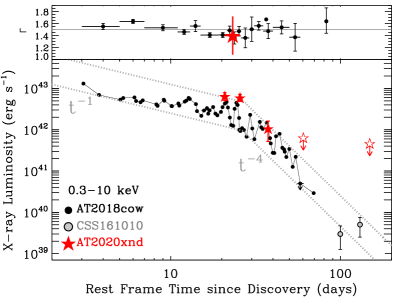
Figure 2: Main Panel: Soft X-ray (0.3-10 keV) luminosity evolution of AT 2020xnd (red stars) compared to the other two known FBOTs with X-ray detections AT 2018cow and CSS 161010 (filled black and grey circles, respectively; Margutti et al. 2019; Coppejans et al. 2020 ). Dotted lines mark a $L_{x}\propto t^{-1}$ and a $L_{x}\propto t^{-4}$ power-law decay to guide the eye. Interestingly, AT 2020xnd shows a similar luminosity as AT 2018cow and seems to follow a similar, peculiar temporal evolution, with roughly constant X-ray flux at $\delta t\leq 30$ d followed by a sharp decay. Upper panel: spectral photon index evolution with time for AT 2018cow and AT 2020xnd. The solid horizontal line is a photon index of 1.5.

2.2.1 Chandra X-ray Observatory (0.3-10 keV)

We acquired deep X-ray observations of AT 2020xnd with the Chandra X-ray Observatory (CXO) under a joint CXO-NuSTAR program #22500192 (PI Matthews; IDs 23547, 23548, 23549; exposure time of $\approx$19.8 ks per ID) covering the time period $\delta t=25-240\,\rm{d}$. We reduced the ACIS-S data with the CIAO software package (v4.12) and relative calibration files (CALDB 4.9.3), applying standard ACIS data filtering (Fruscione et al., 2006).

We refined the CXO absolute astrometry by cross-matching the 0.5-8 keV X-ray sources blindly detected with wavdetect with optical sources in SDSS DR9. After the re-alignment we find evidence for statistically significant X-ray emission at coordinates RA=$22^{\rm{h}}20^{\rm{m}}02^{\rm{s}}.036\pm 0^{\rm{s}}.078$ and $\delta=-02^{\circ}50$′$25$″$.34\pm 0$″$.11$, which is consistent with the optical and radio position of AT 2020xnd. The measured source count-rates and the detection significance are reported in Table 3. At $\delta t_{rest}<25.6\,\rm{d}$ (rest frame) the X-ray source shows roughly constant flux. The source experienced significant fading at $\delta t_{rest}\geq 26\,\rm{d}$, and the flux decays as $F_{x}\propto t^{-\alpha}$ with $\alpha\approx 4.5$ (Figure 2). This very steep late-time X-ray flux decay is similar to AT 2018cow (Figure 2), which is the only other FBOT with X-ray observations at these epochs (Margutti et al., 2019; Rivera Sandoval et al., 2018). These properties make AT 2020xnd the third FBOT with luminous X-ray emission $L_{x}>10^{42}\,\rm{erg\,s^{-1}}$ (Figure 2) and the third with detected X-rays (Margutti et al., 2019; Coppejans et al., 2020).

For each of the first three CXO epochs we extracted a spectrum with specextract using a 1″  region around the X-ray source and a source-free region of 33″  for the background. The neutral hydrogen column density in the direction of the transient is $\rm{NH_{MW}}=4.8\times 10^{20}\,\rm{cm^{-2}}$ (Kalberla et al., 2005). We modeled each spectrum with an absorbed power-law model (tbabs*ztbabs*pow within Xspec; Arnaud 1996). We found no statistical evidence for spectral evolution. We thus proceeded with a joint spectral fit. The best fitting power-law photon index is $\Gamma=1.40^{+0.33}_{-0.32}$ and we place a 3 $\sigma$ limit on the intrinsic absorption column of $\rm{NH_{int}}<3\times 10^{22}\,\rm{cm^{-2}}$. The corresponding 0.3–10 keV fluxes and luminosities are reported in Table 3. We found no evidence for statistically significant X-ray emission at $\delta t_{rest}>60\,\rm{d}$ and we place upper limits on the source count-rate of $\lesssim 10^{-4}\,\rm{c\,s^{-1}}$ (0.5–8 keV) assuming Poissonian statistics as appropriate in the regime of low count statistics. This leads to luminosity limits $L_{x}<(0.3-0.6)\times 10^{42}\,\rm{erg\,s^{-1}}$ using the spectral parameters and model that best fits the earlier observations (Table 3).

2.2.2 NuSTAR (3-79 keV)

We observed AT 2020xnd using the Nuclear Spectroscopic Telescope Array (NuSTAR, 3-79 keV) under the joint CXO-NuSTAR program (PI Matthews; program 22500192; IDs 80701407002, 80701407004, 80701407006; Table 4). We reduced the data with NuSTARDAS (v1.9.2) and relative calibration files. We centered a source extraction aperture of 1′  at the CXO coordinates and we estimated the background using an annulus of inner and outer radii of 1.1′and 3′, respectively. Using Poissonian statistics, we found no evidence for significant emission above the background in the source region. The resulting 3–79 keV count-rate, flux and luminosity limits are listed in Table 4. We adopt a power-law spectral model with photon index $\Gamma=1.5$ and a counts-to-flux factor of $1.5\times 10^{-10}$ for the spectral calibration. We find $L_{x}<5\times 10^{43}\,\rm{erg\,s^{-1}}$ (3–79 keV) in the time range probed by our observations, which corresponds to $\delta t_{rest}=T_{0}+25$ to $T_{0}+52$d. For comparison, the hard X-ray Compton hump was detected in AT 2018cow with hard X-ray luminosities $\approx 10^{43}\,\rm{erg\,s^{-1}}$ at $\delta t_{rest}<15\,\rm{d}$ (Margutti et al., 2019).

Figure 3: Radio observations of AT 2020xnd taken with the VLA, ATCA, GMRT, GBT, MeerKAT, ALMA, AMI-LA, and eMERLIN radio telescopes, with best fits shown for the model described in §3.2. Curves are plotted at the mean time of the observations within the time ranges described in the legend. (a) Our best sampled radio SED, without considering any evolution of the break flux and frequency. (b) All radio observations of AT 2020xnd. The model fit describes the single epoch data well. When considering the entire data set it is clear that the evolving SED model is in marginal contention with the late-time low frequency data from MeerKAT at $\delta t>191$d, over-predicts data at $\delta t=T_{0}+148$d and $\delta t=T_{0}+167$d, while under-predicting the epoch at $\delta t=T_{0}+75\,\rm{d}$. (c) Radio observations at $\delta t\leq T_{0}+75$d. The best fit model parameters and the inferred physical parameters for the data subsets in (a), (b) and (c) are given in Table 5 and Table 6, respectively.

3 Results

3.1 General Considerations

AT 2020xnd shows a roughly constant X-ray luminosity at $\delta t_{rest}\leq 30\,\rm{d}$ followed by a sharp decline, which was similarly seen in the FBOT AT2018cow (Figure 2) Also shown in Figure 2 is the X-ray photon index of AT 2020xnd. The measured soft X-ray spectral index $\beta_{x}=0.4^{+0.33}_{-0.34}$ (where $F_{\nu}\propto\nu^{-\beta_{x}}$, §2.2.1) is shallower than expected from optically thin synchrotron emission above the cooling break frequency $\nu_{c}$ (§3.5). In this regime, $F_{\nu}\propto\nu^{-p/2}$ (e.g., Granot & Sari 2002), where $p$ is the index of the power-law distribution of relativistic electrons with Lorentz factor $\gamma_{e}$ ($N_{e}(\gamma_{e})\propto\gamma_{e}^{-p}$). For relativistic shocks of long/short GRBs and the Newtonian shocks of SNe $p\approx 2-3$ (see e.g. Chevalier & Fransson 2006; Fong et al. 2019) hence $F_{\nu}\propto\nu^{-\beta}$ with $\beta=1-1.5$. This again is similar to what was seen in AT2018cow (Margutti et al., 2019). While our NuSTAR observations probe the hard X-rays ($3-79$ keV), the large distance of AT 2020xnd only allows us to place upper limits in this region of the spectrum that are comparable to the luminosity of the observed Compton hump in AT 2018cow. However, since NuSTAR observations of AT 2020xnd started at $\delta t_{rest}=25$d, which is after the Compton hump component faded away in AT 2018cow, we cannot rule out that AT 2020xnd exhibited a hard X-ray excess similar to the one seen in AT 2018cow at earlier times (Margutti et al., 2019).

Figure 3 shows the evolving radio SED of AT 2020xnd for different subsets of our radio data. At early times ($\delta t\lesssim T_{0}+30$d) the emission is optically thick up to at least $\nu\sim 90\,\rm{GHz}$, with a spectral index of $\sim 1.4$ below the break. The peak of the SED moves to lower flux density with time, while moving to a lower frequency, until we clearly see the peak in our data at $\delta t\approx T_{0}+75$d. The optically thin spectral index is not constrained by our data. This spectral shape is similar to the one expected from self-absorbed synchrotron emission, albeit with a flatter self-absorption spectral index (which is expect to be $\sim 2$ or $\sim 2.5$). The evolution of the break and peak flux suggest the radio emission is from an evolving emitting region that expands and becomes optically thin to lower frequencies with time. This can be interpreted as the result of ejecta material from AT 2020xnd interacting with the CSM surrounding the progenitor. The flatter optically thick slope that we measure could be the result of scintillation effects, however we disfavor this due to the smoothness of the radio SEDs. We are unable to check for short timescale variability or extreme in-band spectral indices (both features of scintillation) due to the low measured flux density of AT 2020xnd at low frequencies.

3.2 Radio SEDs modeling

First, we focus on our radio observations at $\delta t\approx T_{0}+75$d where the peak of the SED is best sampled. We employ the smoothed broken power-law SED model of Equation 1:

$$F(\nu,t)=F_{p}(t)\Bigg{[}\bigg{(}\frac{\nu}{\nu_{b}(t)}\bigg{)}^{-b_{1}/s}+\bigg{(}\frac{\nu}{\nu_{b}(t)}\bigg{)}^{-b_{2}/s}\Bigg{]}^{-s},$$ (1)

where $\nu_{\rm{b}}$ is the break frequency, $F_{p}$ is the peak flux density at which the asymptotic power-law segments meet, $s>0$ is a smoothing parameter, $b_{1}$ and $b_{2}$ are the optically thick and optically thin asymptotic spectral indexes, respectively, at $\nu\ll\nu_{b}$ and $\nu\gg\nu_{b}$. Adopting $s=1$ and $b_{2}=-1$ as typically observed in SNe in the optically thin regime (Chevalier & Fransson, 2006), we find $F_{p}=960\pm 70\,\mu\rm{Jy}$ and $\nu_{b}=35\pm 7\,\rm{GHz}$, respectively, at $T_{0}+75$d.

Next we attempt to model the entire radio data set shown in panel (b) of Figure 3 assuming a power-law evolution in time of the break frequency ($\nu_{b}(t)=\nu_{b,0}(t/T_{0})^{-\alpha_{\nu}}$) and peak flux density ($F_{p}(t)=F_{p,0}(t/T_{0})^{-\alpha_{F}}$), where our reference epoch is $T_{0}+75\,\rm{d}$. We assume constant spectral indexes $b_{1}$ and $b_{2}=-1$, and a common $s=1$. Fitting all of our radio data with in this framework leaves five free parameters: $F_{p,0}$, $\alpha_{F}$, $\nu_{b,0}$, $\alpha_{\nu}$, and $b_{1}$. As shown in panel (b) of Figure 3 this model is unable to satisfactorily fit the entire set of radio observations. The model under-predicts the peak flux at our best sampled epoch, while over-predicting the later-time data (especially at frequencies close to $10$GHz while being in marginal contention with lower frequency data). This is not unprecedented for FBOTs. AT2018cow also demonstrated a significant change in its radio evolution at $\approx 20$d, with the flux density dropping off markedly faster than predicted by an extrapolation of fits to the early-time data (Margutti et al., 2019). We were able to achieve better fitting results when using only the subset of our data at $\delta t\leq T_{0}+75$d, with the results shown in panel (c) of Figure 3 and the best fit model parameters given in Table 5. In the following discussion we adopt the model parameters derived for the fits to the subset of data taken at and before $\delta t\sim T_{0}+75\,\rm{d}$ (Figure 3 panel (c)) when inferring physical parameters. This allows us to better compare with our CXO observations (which were taken before $75$d), and account for our best sampled radio SEDs. We will discuss possible interpretations of the late time ($\delta t>T_{0}+75$d) radio flux in §4.2.

3.3 Physical Parameters at $\delta t\lesssim T_{0}+75\,\rm{d}$

Using the results of our fitting in §3.2 we can infer physical parameters of the emitting region based on some simple assumptions. Following Chevalier & Fransson (2006), we calculate the forward shock radius $R_{p}$, the magnetic field $B_{p}$, the density of the CSM $n$, and the shock energy $U_{p}$, all as a function of time and accounting for the significant redshift of AT 2020xnd (which we describe in more details in Appendix A). We further adopt fiducial values for the shock microphysical parameters of $\epsilon_{e}=0.1$, $\epsilon_{B}=0.01$, and an emitting volume fraction $f=0.5$ (compared to a sphere of radius $R_{p}$). We let $\alpha\equiv f\epsilon_{e}/(0.5\epsilon_{B})$, which encapsulates the main assumptions of our model.

The radius of the forward shock is

$$\begin{split}R_{p}=4&\times 10^{14}\alpha^{-\frac{1}{19}}\bigg{(}\frac{F_{p}(1+z)^{-1}}{\rm{mJy}}\bigg{)}^{\frac{9}{19}}\bigg{(}\frac{D_{\theta}}{\rm{Mpc}}\bigg{)}^{\frac{18}{19}}\\ \times&\bigg{(}\frac{\nu_{b}(1+z)}{5\,\rm{GHz}}\bigg{)}^{-1}\,\rm{cm},\end{split}$$ (2a)

while its temporal evolution is modeled as:

$$R_{p}=R_{p,0}\bigg{(}\frac{t}{T_{0}}\bigg{)}^{\alpha_{\nu}-(9/19)\alpha_{F}}=R_{p,0}\bigg{(}\frac{t}{T_{0}}\bigg{)}^{1.0\pm 0.1}.$$ (2b)

Here $R_{p,0}=(2.8\pm 0.2)\times 10^{16}$cm is the value of $R_{p}$ at our reference time (which we take to me $\delta t=T_{0}+75$d post explosion). We give statistical errors on the derived scalings, as well as the physical parameters, based on propagating the errors derived from our model fitting. We note, however, that systematic errors resulting from the model assumptions likely dominate. We can then infer the average velocity implied by our model as $(\beta\Gamma c)_{p}=(R_{p}(1+z)/t_{0})$ (which is $0.18\pm 0.02$ at $75\,\rm{d}$ post explosion). The best fit model to these data is consistent with no acceleration ($R_{p}\propto t^{1.0\pm 0.1}$), although we only confidently measure the location of the peak at the reference epoch. As a comparison, fitting only the data at $\delta t=T_{0}+75$d, we infer a shock radius of $(2.0\pm 0.7)\times 10^{16}\,\rm{cm}$ at this epoch, implying an average outflow velocity of the fastest ejecta of $\Gamma\beta c=R(1+z)/t=0.13\pm 0.04$. Note that the dependency on the shock microphysical parameters is minor, with an order of magnitude change in $\alpha$ resulting in a $\sim 10\%$ change in the radius and velocity (see Equation 2a).

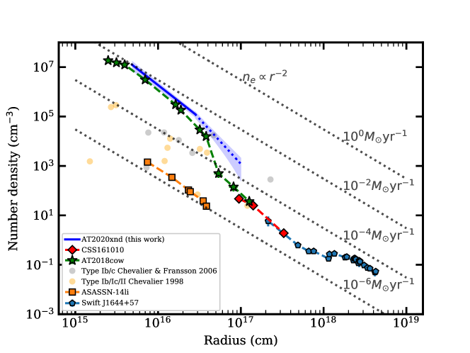
Figure 4: The particle number density as a function of radius for the FBOTs AT2020xnd including the possible steepening at $\delta t\sim T_{0}+75$d (this work), CSS161010 (Coppejans et al., 2020) and AT2018cow (Margutti et al., 2019; Nayana & Chandra, 2018; Ho et al., 2019c). Also shown are single measurements from various Type Ib/c and Type II SNe where we derived the number density using values from Chevalier & Fransson (2006) and Chevalier (1998). Additionally, we include number density measurements from the prototypical thermal and non-thermal TDEs, ASASSN-14li and SwiftJ1644+57, respectively (Alexander et al., 2016; Eftekhari et al., 2018). Note that the densities derived for the two TDEs used the results of Barniol Duran et al. 2013 as opposed to Chevalier & Fransson 2006 in this work. Dotted gray lines show different rates of constant mass loss ($n_{e}\propto r^{-2}$ and assuming a wind velocity of $1000$km s^-1). FBOTs show preferentially high densities and therefore larger mass loss rates compared to the type-Ibc/Ic/II events presented in Chevalier (1998) and Chevalier & Fransson (2006).

The magnetic field and its scaling are given in Equation 3a and Equation 3b, respectively:

$$\begin{split}B_{p}=1.1&\alpha^{-\frac{4}{19}}\bigg{(}\frac{F_{p}(1+z)^{-1}}{\rm{mJy}}\bigg{)}^{-\frac{2}{19}}\bigg{(}\frac{D_{\theta}}{\rm{Mpc}}\bigg{)}^{-\frac{4}{19}}\\ \times&\bigg{(}\frac{\nu_{b}(1+z)}{5\,\rm{GHz}}\bigg{)}\,\rm{G}\end{split}$$ (3a)

$$B_{p}=B_{p,0}\bigg{(}\frac{t}{T_{0}}\bigg{)}^{(2/19)\alpha_{F}-\alpha_{\nu}}=B_{p,0}\bigg{(}\frac{t}{T_{0}}\bigg{)}^{-1.3\pm 0.1}$$ (3b)

Here $B_{p,0}$ is the value of $B_{p}$, the magnetic field associated with the self-absorbed synchrotron emission, at our references time. Note again that, similar to the radius, the value of the magnetic field is relatively robust to the choice of $\alpha$. We find $B_{p,0}=1.04\pm 0.07$G. Fitting the SED at $\delta t=T_{0}+75\,\rm{d}$ in isolation we find a post-shock magnetic field of $1.5\pm 0.3\,\rm{G}$. These values are similar to those of SNe and other FBOTs (e.g., Chevalier & Fransson 2006; Ho et al. 2020c; Margutti et al. 2019; Coppejans et al. 2020).

Additionally, the peak flux and break frequency allow us to constrain a density profile for the CSM, which was crafted by the mass loss history of the progenitor star, that the SN outflow is interacting with. The density profile of the CSM can be written as $\rho=\dot{M}/(4\pi r^{2}v_{w})=Ar^{-2}$, where $\dot{M}$ is the mass-loss rate of the star with wind of velocity $v_{w}$. We define $A_{\star}\equiv A/(5\times 10^{11}\,\rm{g}\,\rm{cm}^{-1})$ so that $A_{\star}=1$ for $\dot{M}=10^{-5}M_{\odot}\rm{yr}^{-1}$ and $v_{w}=1000\,\rm{km}s^{-1}$, which are typical of Wolf-Rayet stars. Under the assumption that a fraction $\epsilon_{B}$ of the shock energy density is converted to magnetic energy density, $A_{\star}$ can be defined as in Equation 4a and the scaling resulting from our models as in Equation 4b.

$$\begin{split}A_{\star p}=&\alpha^{-\frac{8}{19}}\bigg{(}\frac{\epsilon_{B}}{0.1}\bigg{)}^{-1}\bigg{(}\frac{F_{p}(1+z)^{-1}}{\rm{mJy}}\bigg{)}^{-\frac{4}{19}}\bigg{(}\frac{D_{\theta}}{\rm{Mpc}}\bigg{)}^{-\frac{8}{19}}\\ &\times\bigg{(}\frac{\nu_{b}(1+z)}{5\,\rm{GHz}}\bigg{)}^{2}\bigg{(}\frac{t(1+z)^{-1}}{10\,\rm{d}}\bigg{)}^{2}\end{split}$$ (4a)

$$A_{\star p}=A_{\star p,0}\bigg{(}\frac{t}{t_{0}}\bigg{)}^{(4/19)\alpha_{F}-2\alpha_{\nu}+2}=A_{\star p,0}\bigg{(}\frac{t}{t_{0}}\bigg{)}^{-0.5\pm 0.2}$$ (4b)

For the best fit parameters of our model we find that $A_{\star p,0}=(90\pm 10)\times\alpha^{-8/19}(\epsilon_{B}/0.1)^{-1}$ or $A=(1.8\pm 0.2)\,\times 10^{13}\,\rm{g}\,\rm{cm}^{-1}$ for $\alpha=10$. Using the scaling derived in Equation 2b we see that, under the assumption that the CSM is dominated by fully ionized hydrogen, the number density profile is:

$$n\bigg{(}\frac{R_{p}}{R_{p,0}}\bigg{)}=5\times 10^{11}m_{p}^{-1}\bigg{(}\frac{A_{\star p,0}}{R_{p,0}^{2}}\bigg{)}\bigg{(}\frac{R_{p}}{R_{p,0}}\bigg{)}^{\frac{22\alpha_{F}-76\alpha_{\nu}+38}{19\alpha_{\nu}-9\alpha_{F}}}\,\rm{cm}^{-3},$$ (5)

and therefore $n=n_{p,0}(R_{p}/R_{p,0})^{-2.5\pm 0.2}$. From the previously calculated values of $A_{\star p,0}$ and $R_{p,0}$, we see that $n_{p,0}=(1.2\pm 0.2)\times 10^{4}\,\rm{cm}^{-3}$ at a radius of $R_{p}\sim 2.8\times 10^{16}\,\rm{cm}$ (i.e. $R_{p,0}$). These values imply effective mass-loss rates $\dot{M}\sim 3\times 10^{-3}\,M_{\odot}\rm{yr}^{-1}$ for $v_{w}=1000\,\rm{kms}^{-1}$. We compare the density profile of AT 2020xnd with other classes of SNe and FBOTs in Figure 4. The inferred density of the environment of AT2020xnd is very similar to that of the FBOT AT2018cow, and denser than typical SN environments. While similarly large densities can be found around supermassive black holes (SMBHs), dormant intermediate-mass BHs are not expected to be surrounded by high-density media. This provides challenges for FBOT models invoking a TDE around an IMBH (e.g., Kuin et al. 2019; Perley et al. 2019). By the end of our observing campaign we are probing emission at $\sim 10^{17}$cm. Taking our number density profile and integrating it out to this radius implies a total mass swept up of $\sim 10^{-2}\rm\rm{M_{\odot}}$.

Finally, we calculate the shock energy according to

$$\begin{split}U_{p}=&\bigg{(}\frac{fR^{3}B^{2}}{6\epsilon_{B}}\bigg{)}=1.3\times 10^{43}f\epsilon_{B}^{-1}\alpha^{-\frac{11}{19}}\bigg{(}\frac{F_{p}(1+z)^{-1}}{\rm{mJy}}\bigg{)}^{\frac{23}{19}}\\ &\times\bigg{(}\frac{D_{\theta}}{\rm{Mpc}}\bigg{)}^{\frac{46}{19}}\bigg{(}\frac{\nu_{p}(1+z)}{5\,\rm{GHz}}\bigg{)}^{-1}\,\rm{erg}\end{split}$$ (6a)

$$U_{p}=U_{p,0}\bigg{(}\frac{t}{t_{0}}\bigg{)}^{\alpha_{\nu}-(23/19)\alpha_{F}}=U_{p,0}\bigg{(}\frac{t}{t_{0}}\bigg{)}^{0.5\pm 0.3}$$ (6b)

and find that, $U_{p}=(1.5\pm 0.1)\times 10^{49}f\epsilon_{B}^{-1}\alpha^{-11/19}\,\rm{erg}$ or $U_{p}=(2.0\pm 0.2)\times 10^{50}$erg, for our fiducial $f$, $\alpha$ and $\epsilon_{B}$ parameters. For comparison, the single 75d-SED fit returned a total shock energy of $U=(1.5\pm 0.4)\times 10^{50}\,\rm{erg}$. For comparisons, AT2018cow showed significantly less energy ($U\sim 5\times 10^{47}$erg) at similar epochs (Margutti et al. 2019, Coppejans et al., in prep.), while the mildly relativistic FBOT CSS161010 was powered by a similarly energetic outflow with $U=(2.9\pm 0.1)\times 10^{49}$erg (Coppejans et al., 2020).

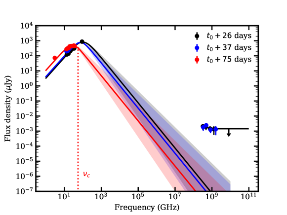
Figure 5: The radio through X-ray SED of AT 2020xnd showing our two Chandra epochs and the two nearest-in-time VLA epochs. Also shown is the reference epoch where we best sample the peak of the radio SED. Under the assumption that the peak of the SED is the result of synchrotron self-absorption we estimate the location of the synchrotron cooling break, $\nu_{c}$, at the reference epoch, and demonstrate this here. Due to the magnetic field scaling derived in Section 3.5 the cooling break should move to higher frequencies with time. At the black and blue epochs we are in the regime where $\nu_{m},\nu_{c}<\nu_{sa}$, and the cooling break is not seen. Instead we show these epochs with the slope post self absorption frequency steepened from $-(p-1)/2$ to $-p/2$. The wide upper limit given at epoch 1 is from NuSTAR and includes the entire 3 to $79$keV observing band. Constraints at the other epochs were comparable. While we fix the post-break spectral index to -1 in our model, the shaded regions show the effect of including an error of $\pm 0.3$ on this value.

3.4 Late time emission at $\delta t>75\,\rm{d}$: sub-mm and low frequency constraints

As discussed in the previous sections, a single power-law evolution of the peak flux and peak frequency with time is unable to provide an accurate representation of the entire data set. Our data coverage is sparser at $\delta t>T_{0}+75\,\rm{d}$, however the data indicate a significantly faster evolution. In this time range we find $\alpha_{\nu}=2.1\pm 0.4$ and $\alpha_{F}=2.2\pm 0.2$, which we calculate by fitting just the SEDs at $\delta t=T_{0}+75$d and $\delta t=T_{0}+148$d. Interestingly, these imply a steepening of the density profile as $n\propto(R/R_{0})^{3.6\pm 0.6}$ around $R_{p}\sim 3\times 10^{16}$cm. A similar steepening was inferred for the environment of AT2018cow and might represent a defining characteristics of the class of luminous FBOTs. We will discuss possible origins of this density profiles in §4.2.

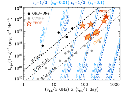
Figure 6: Left Panel: Radio phase-space of stellar explosions, where $L_{\rm{\nu,pk}}$ is the spectral peak luminosity, $\nu_{\rm{pk}}$ is the spectral peak frequency and $t_{\rm{pk}}$ is the peak time. Normal core-collapse stellar explosions (CCSNe, gray filled circles) typically show a shock velocity $\sim 0.1$c, while GRB-SNe (Black filled circles) are characterized by significantly faster shocks. The new class of multiwavelength FBOTs (stars) is currently comprised of four elements and shows a variety of shock velocities that bridge the gap between normal SNe (e.g., AT 2018cow) and the ultra-relativistic jets of GRBs (e.g., CSS 161010, AT 2018lug and AT 2020nxd). Dashed dark (dotted light) blue lines: lines of constant equivalent mass-loss rate for an assumed wind velocity $v_{w}=1000\,\rm{km\,s^{-1}}$ for equipartition parameters $\epsilon_{B}=\epsilon_{e}=1/3$ ($\epsilon_{B}=0.01$, $\epsilon_{e}=0.1$). Black dashed lines: lines of constant apparent velocity $R/\Delta t$ under the assumption of equipartition. The factor $(1+z)^{-3}$ accounts for the difference between the angular distance and the luminosity distance. Right Plot: Shock energy vs. fastest ejecta velocity for a variety of transients, including TDEs, SNe and FBOTs. FBOTs represent a new class of transients with energetic shocks that can be transrelativistic. Among FBOTs, AT2020xnd shows the largest equipartition energy. Same color coding as panel on the left. Shaded region: parameter space of engine driven explosions. References: Margutti et al. (2019); Ho et al. (2019c); Coppejans et al. (2020).

3.5 Synchrotron Cooling

The frequency of the cooling break (where the electrons are radiating a significant fraction of their energy to synchrotron radiation on a dynamical timescale) can be estimated as $\nu_{c}=(18\pi m_{e}ce)/(t^{2}\sigma_{t}^{2}B^{3})$ where we can use our estimates for the magnetic field made in the previous section. For our best fit model parameters (for data taken at $\delta t\leq T_{0}+75\,\rm{d}$) we see that $\nu_{c}=\nu_{c,0}(t/t_{0})^{1.6\pm 0.4}\,\rm{GHz}$, with $\nu_{c,0}=(70\pm 10)\,\rm{GHz}$ (we stress however that these calculations are only strictly valid for a constant magnetic field and depend quite strongly on $\alpha$). At the same time the synchrotron frequency is $\nu_{m}\equiv\gamma_{m}^{2}\big{(}\frac{eB}{2\pi m_{e}c}\big{)}\approx 3\gamma_{m}^{2}$MHz, so we have that $\nu_{m}<\nu_{sa}<\nu_{c}$ for $\gamma_{m}\lesssim 170$. The synchrotron spectrum from a population of electrons accelerated into a power-law distribution with an index $p$ governing their energy distribution steepens from $F_{\nu}\propto\nu^{-(p-1)/2}$ to $F_{\nu}\propto\nu^{-p/2}$ above the cooling break (in the event that $\nu_{sa}<\nu_{m}<\nu_{c}$ or $\nu_{m}<\nu_{sa}<\nu_{c}$, see e.g. Granot & Sari 2002).

We show the cooling break in the context of the radio through X-ray SED in Figure 5 for data taken at our reference epoch, along with the two epochs with quasi-simultaneous CXO and radio observations. At early times $\nu_{c}<\nu_{sa}$ (which might be contributing to “broadening” the synchrotron cooling break) and the optically-thin spectrum never demonstrates the $F_{\nu}\propto\nu^{-(p-1)/2}$ scaling, instead moving directly to the $F_{\nu}\propto\nu^{-p/2}$ regime. Accounting for the presence of synchrotron cooling demonstrates that the X-rays are in a significant excess to the radio data taken at approximately the same time, as found for the other FBOTs with both radio and X-ray data, CSS161010 and AT2018cow (Coppejans et al. 2018; Margutti et al. 2019). The presence of a luminous X-ray excess of emission appears to be a defining property of optically-luminous FBOTs (further discussed in §4.1).

4 Discussion

4.1 An X-ray Excess

We detected AT 2020xnd on three epochs with the Chandra X-ray Observatory, with a significant drop occurring between the our second and third observations (see Figure 2). We show the radio through X-ray SED of AT 2020xnd in Figure 5, demonstrating the location of the cooling break at various epochs. It is clear that, as for the other two FBOTs with both X-ray and and radio detections, the extrapolated radio spectrum predicts less X-ray emission than observed. This is the case even considering relatively large error on the post break spectral index. From our Chandra observations of AT 2020xnd we can measure the photon index to be $\Gamma=\beta+1=1.4^{+0.33}_{-0.33}$. This is shallower (harder) spectral than we would expect for the fast cooling regime in the X-rays ($\Gamma=2$ to $2.5$), further suggesting a different origin for the X-ray emission in addition to (and consistent with) our assessment based on the X-ray flux level. Similar considerations based on similar observational evidence, led Margutti et al. (2019) to suggest the presence of a centrally-located source of hard X-ray emission in AT2018cow.

In stark contrast to normal SNe (see e.g., SN2014C; Margutti et al. 2017), the X-ray emission in AT2018cow is of clear non-thermal origin (Margutti et al., 2019). An intriguing possibility is that the source of energy of AT2018cow might be connected to energy released by a newly-formed compact object, either in the form of a black-hole or neutron star. With $L_{x}\approx 6\times 10^{42}\,\rm{erg\,s^{-1}}$ (Figure 2), the measured X-ray luminosity of AT 2020xnd is $\approx$5 orders of magnitude larger than the Eddington luminosity for a stellar mass black hole (see Table 3). This is similar to what was seen in the FBOTs AT2018cow and CSS161010 (Margutti et al. 2019; Coppejans et al. 2018), confirming that FBOTs with associated X-ray emission have a similar luminosity to TDEs and GRBs in the local universe, and are significantly more luminous than “normal” CCSNe (see e.g., Margutti et al. 2013a, b; Drout et al. 2014; Vinkó et al. 2015; Margutti et al. 2017; Eftekhari et al. 2018 for luminosities of these various transient classes).

If the X-ray emission from FBOTs is powered by a nebula of relativistic particles energized by a central engine, the sudden drop in the X-ray luminosity could in principle arise from an abrupt shift in the spectral energy distribution of the emission rather than change in the bolometric decay of the engine’s luminosity (which is generally predicted to be smooth in fall-back accretion or magnetar-powered scenarios). For example, in their recent self-consistent Monte Carlo calculations of jet/magnetar-powered nebulae and engine-powered transients, Vurm & Metzger (2021) predict that, for FBOT-scaled engine and ejecta properties, an abrupt increase in the mean particle per energy is predicted to occur on a timescale of $\sim 1$ month after the explosion due to a change in the processes regulating the mass-loading of the wind/jet (namely, the cessation of $\gamma\gamma$ pair production). The resulting sudden increase in the peak of the non-thermal synchrotron or inverse Compton emission could act to shift the radiated energy from the soft X-ray to the gamma-ray band (where it would go undetected at these relatively late epochs).

4.2 Late Time Radio Emission

Interestingly, as with the other radio-loud FBOTs with well monitored radio emission, we were not able to describe the entire data set of AT 2020xnd with an evolving broken power-law as described by Equation 1 (Margutti et al. 2019; Coppejans et al. 2020; Coppejans+ in prep.). This is the result of a sharp late-time drop-off in radio flux that we speculate is a defining characteristic of FBOTs. In normal SNe, $F_{p}$ tends to remain constant in time, while $\nu_{p}\propto t^{-1}$, which leads to the characteristic $F_{\nu}\propto t^{-1}$ in the optically thin regime that is appropriate at these late epochs. The markedly different rate of decay of the radio flux density of FBOTs vs. normal SNe after peak can be immediately appreciated from Figure 2. From a physical perspective, this fast evolution can be the result of a steeply decaying environment density at larger radii, moving from $\rho\propto(R/R_{0})^{2.5\pm 0.2}$ at $\delta t\lesssim T_{0}+75$d to $\rho\propto(R/R_{0})^{3.6\pm 0.6}$ afterwards (determined by fitting the evolution between the SEDs at $\delta t=T_{0}+75$d and $\delta t=T_{0}+148$d (see Figure 4). This is inferred from the peak flux density decaying faster at later times ($\alpha_{F}=0.7\pm 0.1$ to $\alpha_{F}=2.2\pm 0.2$), and the break frequency moving faster to lower frequencies ($\alpha_{\nu}=1.3\pm 0.1$ to $\alpha_{\nu}=2.1\pm 0.4$). However, we emphasize that in the context of our synchrotron formalism where the shock microphysics parameters are constant with time, an equivalent interpretation of the steeply decaying $F_{p}(t)$ and $\nu_{p}(t)$ parameters would be that of a rapidly evolving $B(R)$. The fast evolution could also be the result of a decelerating blastwave, however the large errors when jointly fitting the $\delta t=T_{0}+75$d and $\delta t=T_{0}+148$d SEDs prevent us from determining the radius evolution between these epochs.

4.3 Free-Free Absorption

Due to the high environment densities we derive based on our radio SED modelling, we consider the potential effects of free-free absorption on the observed radio SED which would manifest as a sharp drop-off at low frequencies (and hence and optically thick flux density $F_{\nu}\propto\nu^{\beta}$ with $\beta>5/2$; e.g., Weiler et al. 2002). Our SED do not show any evidence for free-free absorption. Following Margutti et al. 2019 we have that the optical depth to free-free absorption is

$$\begin{split}\tau_{\rm{ff}}\approx&\frac{\alpha_{\rm{ff}}r}{3}\approx 10\bigg{(}\frac{\nu}{10\,\rm{GHz}}\bigg{)}^{-2}\bigg{(}\frac{T_{g}}{10^{4}\,\rm{K}}\bigg{)}^{-3/2}\bigg{(}\frac{\rm{A}}{100\rm{A_{\star}}}\bigg{)}^{2}\\ &\times\bigg{(}\frac{v}{0.1c}\bigg{)}^{-3}\bigg{(}\frac{t}{\rm{wk}}\bigg{)}^{-3}.\end{split}$$ (7)

Here $\alpha_{\rm{ff}}$ is the absorption coefficient of free-free absorption, $T_{g}$ is the temperature of the absorbing gas, and $v$ is the shock velocity. The subset of our data at $t\lesssim T_{0}+76\,\rm{d}$ shows a spectral index broadly consistent with synchrotron self-absorbed emission (although with a shallower self-absorption index than the expected $F_{\nu}\propto\nu^{2}$ for $\nu_{m}<\nu<\nu_{sa}$). Free-free absorption will become prevalent when $\tau_{\rm{ff}}\gtrsim 1$, so the lack of any obvious spectral drop-off at low frequencies in any of our epochs implies that $\nu_{\rm{ff,\tau=1}}\ll\nu_{p}$. Using the epoch at $t=T_{0}+75\,$d this implies $\nu_{\rm{ff,\tau=1}}\ll 40\,\rm{GHz}$.

We can then use this observational constraint and Equation 7 to place a constraint on the environment density as

$$\frac{A}{A_{\star}}\lesssim 300\bigg{(}\frac{T_{g}}{10^{4}}\bigg{)}^{3/4}v_{0.1}^{3/2}$$ (8)

at $t=T_{0}+75\,$d. This is consistent with the values derived in §3.3 for our derived outflow velocities.

4.4 Rapid X-ray decline

We show our Chandra X-ray observations of AT 2020xnd in Figure 2 along with those from CSS161010 and the well sampled AT2018cow. A striking feature of the X-ray emission is the significant increase in the rate of flux decay seen at $\sim 20\,\rm{d}$ post discovery (in the target’s rest frame). AT2018cow initially declined according to $F_{x}\propto t^{-1}$ before a steepening occurred changing the decay rate to $F_{x}\propto t^{-4.5}$. The optical properties of AT2018cow appeared to morph on a similar epoch, with the previously featureless optical spectrum showing H and He emission lines with a corresponding velocity of $\sim 4000\,\rm{kms}^{-1}$, and a high photosphere temperature that showed little evolution (Perley et al. 2021). Based on the optical data presented by Perley et al. (2021), AT 2020xnd appears to show similar properties, although a lack of optical spectra taken around $20\,\rm{d}$ post discovery prevents us from confirming the link between X-ray and optical evolution.

The X-ray fading seen in AT2018cow was in no way smooth, with a high level of variability seen on sub-day timescales (Margutti et al. 2019), however due to the relative faintness of AT 2020xnd we could not perform a similar analysis in this work. Sudden changes in the X-ray properties of engine-powered transients/variables are commonly seen in X-ray binary (XRB) systems as sources transition between accretion states (Fender et al., 2004; Remillard & McClintock, 2006). XRBs, however, have X-ray luminosities (attributed to accretion) at approximately, or considerably less than, the Eddington limit, with changes in the X-ray hardness/luminosity (as well as their radio properties, see e.g., Bright et al. 2020b) seen at $\sim 1\%\,\rm{L}_{\rm{Edd}}$. Due to the extremely high X-ray luminosity of the FBOTs (e.g. many orders of magnitude above the Eddington limit for AT 2020xnd) attributing the evolving X-ray evolution of AT2018cow/AT 2020xnd to a similar mechanism is challenging as accretion rates this large are simply not seen in Galactic transients, with only the ultraluminous X-ray sources exceeding the Eddington limit.

5 Conclusions

AT 2020xnd is now the fourth FBOT to be detected at radio frequencies, and the third at X-rays. Our analysis of the evolving radio and X-ray emission allows us to draw a number of key conclusions on the nature of this object:

• The fastest outflows produced by AT 2020xnd (probed through our radio observations) traveled at a significant fraction of the speed of light ($0.1c$ to $0.2c$), a result that is robust to the subset of data which we fit, and also only weakly depends on the model assumptions.

• Our observations strengthen the case for FBOTs hosting a central engine. Our X-ray observations are both spectrally harder than, and in excess of, extrapolations of our fits to the radio data. This implies a distinct emission component producing X-rays in AT 2020xnd. Despite observing AT 2020xnd in the hard X-ray with NuSTAR we were unable to place meaningful constraints on any hard X-ray excess, as seen in AT2018cow.

• Similar to AT2018cow, the X-ray emission from AT 2020xnd underwent a marked change in its decay rate at $\sim 20\,\rm{d}$ post explosion. While the physical cause of this evolution remains unclear, it motivates further X-ray studies of FBOTs.

• We see a distinct change ($\alpha_{F}=0.7\pm 0.1$ to $\alpha_{F}=2.2\pm 0.2$; $\alpha_{\nu}=1.3\pm 0.1$ to $\alpha_{\nu}=2.1\pm 0.4$) in the late-time evolution of the radio SED from AT 2020xnd, revealed through our inability to find a satisfactory fit to the entirety of our radio observations with a single evolving synchrotron spectrum. Our attempts led to a model under-predicting our most well-sampled radio epoch, and moderately over-predicting the late-time data at low frequencies. A similar phenomena was seen (and more clearly) in AT2018cow (Coppejans+ in prep.).

• We find broad agreement with the results obtained by Ho et al.+2021 for their independent analysis of a separate data set from AT 2020xnd. This includes a similar shock velocity, energy, and steep density profile, with a change in shock properties occurring at around $\delta t=T_{0}+75$d. This change in parameters also prevented them from fitting a single evolving synchrotron self-absorbed SED. Furthermore, they also find X-ray emission in excess of an extrapolation of the radio emission, thus requiring a separate emission component.

These properties continue to solidify FBOTs as a new and distinct class of extragalactic transient with luminous counterparts outside the optical spectrum. As surveys such as ZTF and YSE continue to probe events evolving on short timescales only through extensive multi-wavelength followup will the intrinsic nature of fast blue optical transients be revealed.

Appendix A Cosmological Modification to Chevalier (1998)

FBOTs occupy a unique region of the distance/outflow-velocity parameter space for radio transients. The inferred velocities are distinctly non/mildly-relativistic, significantly less than those associated with the distant GRBs (Barniol Duran et al., 2013) or galactic X-ray binaries (Fender & Bright, 2019) while having redshifts more comparable to the former and so must be accounted for. The measured flux density (specific-flux) in the observer’s frame (non-primed) is related to the specific-luminosity in the source’s rest frame (primed) by $F_{\nu}(\nu)=(1+z)L_{\nu}(\nu^{\prime})/(4\pi D_{L}^{2})$ (this is known as a K correction, see e.g. Meyer et al. 2017; Condon & Matthews 2018) where $D_{L}$ is the luminosity distance and $D_{\theta}=D_{L}(1+z)^{-2}$ is the angular diameter distance. We therefore have that $F_{\nu}(\nu)=(1+z)^{-3}L_{\nu}(\nu^{\prime})/(4\pi D_{\theta}^{2})$, where $\nu^{\prime}=\nu(1+z)$ accounts for cosmological redshift. In Chevalier (1998) the angular extent of the source is given by $\theta=R/D$, which is the definition of the angular diameter distance. We wish to apply cosmological corrections to the observed quantities we use to make physical inferences on the FS properties, which are the frequency of the spectral break, the time since explosion, and the flux density at the spectral break. The frequency and time are simple, and are given as $\nu^{\prime}=\nu(1+z)$ and $t^{\prime}=t(1+z)^{-1}$ (and therefore $\nu t=\nu^{\prime}t^{\prime}$ is independent of redshift). For the flux density we begin with our earlier definition $F_{\nu}(\nu)=(1+z)L_{\nu}(\nu^{\prime})/(4\pi D_{L}^{2})$, i.e. the flux density we measure corresponds to the luminosity at the redshifted frequency $\nu^{\prime}$ with the factor $(1+z)$ accounting for the compressed bandwidth over which the flux density is measured in the observer’s frame. The quantity $F_{\nu}^{\prime}(\nu^{\prime})=L_{\nu}(\nu^{\prime})/(4\pi D_{L}^{2})$ is the flux density of interest for the models of Chevalier (1998), being the flux density measured in the source frame at frequency $\nu^{\prime}$. We therefore have that $F_{\nu}^{\prime}(\nu^{\prime})=F_{\nu}(\nu)(1+z)^{-1}$ where the quantities on the right hand side of the equality are all measurable. Throughout this work we give quantities in the non-primed (observer) frame and provide the appropriate redshift corrections in each formula for clarity.

Appendix B Observations

Table 1: Radio Observations of AT 2020xnd.

Start Date	Centroid MJD	Phasea	Frequency	Bandwidth (GHz)	Flux Densityb	Facility
(dd/mm/yy)		(d)	(GHz)	(GHz)	($\mu$Jy)
22/10/2020	59145.0109	13.01	10	4	$23\pm 5$	VLA
25/10/20	59147.28	15.28	5.5	2	$<60$	ATCA
25/10/20	59147.28	15.28	9	2	$<50$	ATCA
29/10/20	59151.41	19.41	18	4	$110\pm 20$	ATCA
05/11/20	59158.22	26.22	19.09	2	$192\pm 32$	VLA
05/11/20	59158.22	26.22	21.07	2	$209\pm 37$	VLA
05/11/20	59158.22	26.22	23.05	2	$273\pm 41$	VLA
05/11/20	59158.22	26.22	25.03	2	$269\pm 35$	VLA
05/11/20	59158.74	26.74	13.49	3	$122\pm 15$	VLA
05/11/20	59158.74	26.74	16.51	3	$139\pm 16$	VLA
06/11/20	59159.82	27.82	5.07	0.512	$<54$	eMERLIN
07/11/20	59160.09	28.09	90.00c	30	$900\pm 100$	GBT
07/11/20	59160.41	28.41	34	4	$310\pm 20$	ATCA
16/11/20	59169.11	37.11	18.98	2	$304\pm 31$	VLA
16/11/20	59169.11	37.11	20.99	2	$350\pm 31$	VLA
16/11/20	59169.11	37.11	23.01	2	$399\pm 32$	VLA
16/11/20	59169.11	37.11	25.02	2	$433\pm 33$	VLA
16/11/20	59169.14	37.14	12.97	2	$200\pm 23$	VLA
16/11/20	59169.14	37.14	15.00	2	$213\pm 17$	VLA
16/11/20	59169.14	37.14	17.02	2	$262\pm 23$	VLA
19/11/20	59172.27	40.27	18	4	$240\pm 31$	ATCA
24/11/20	59177.09	45.09	9.82	4	$112\pm 15$	VLA
24/11/20	59177.10	45.10	6.22	4	$51\pm 12$	VLA
25/11/20	59178.06	46.06	90.00c	30	$560\pm 60$	GBT
27/11/20	59180.25	48.24	34	4	$490\pm 63$	ATCA
03/12/20	59186.05	54.05	90.00c	30	$360\pm 60$	GBT
15/12/20	59198.59	66.59	5.072	0.512	$<114$	eMERLIN
24/12/20	59207.05	75.05	29.98	2	$451\pm 51$	VLA
24/12/20	59207.05	75.05	31.99	2	$480\pm 58$	VLA
24/12/20	59207.05	75.05	34.01	2	$471\pm 52$	VLA
24/12/20	59207.05	75.05	36.02	2	$451\pm 60$	VLA
24/12/20	59207.07	75.07	18.98	2	$420\pm 33$	VLA
24/12/20	59207.07	75.07	20.99	2	$435\pm 34$	VLA
24/12/20	59207.07	75.07	23.01	2	$444\pm 36$	VLA
24/12/20	59207.07	75.07	25.02	2	$444\pm 34$	VLA
24/12/20	59207.09	75.09	12.98	2	$278\pm 24$	VLA
24/12/20	59207.09	75.09	15.00	2	$317\pm 23$	VLA
24/12/20	59207.09	75.09	17.02	2	$331\pm 25$	VLA
24/12/20	59207.11	75.11	3	2	$73\pm 18$	VLA
26/12/20	59209.26	77.26	18	4	$252\pm 36$	ATCA
19/01/21	59234.61	102.61	5.072	0.512	$86\pm 19$	eMERLIN
09/02/21	59254.36	122.36	1.25	0.4	$<87$	GMRT
07/03/21	59280.69	148.69	33	8	$<72$	VLA
07/03/21	59280.71	148.71	22	8	$70\pm 17$	VLA
07/03/21	59280.73	148.73	15	6	$90\pm 12$	VLA
07/03/21	59280.75	148.75	6.224	4	$99\pm 16$	VLA
18/03/21	59291.44	159.44	15.5	4	$<156$	AMI-LA
21/03/21	59294.33	162.33	0.75	0.4	$<177$	GMRT
23/03/21	59296.33	164.33	1.26	0.4	$<75$	GMRT
26/03/21	59299.77	167.77	3	2	$<105$	VLA
26/03/21	59299.78	167.78	9.824	4	$49\pm 19$	VLA
26/03/21	59264.80	167.80	6.224	4	$44\pm 22$	VLA
12/04/21	59316.48	184.48	97.49	8	$<42$	ALMA
12/04/21	59316.53	184.53	144.99	8	$<45$	ALMA
16/03/21	59323.94	191.94	15.5	4	$<135$	AMI-LA
19/04/21	59323.18	191.18	1.28	0.856	$<60$	MeerKAT
23/04/21	59327.28	195.28	5.072	0.512	$<60$	eMERLIN
29/05/21	59363.33	231.33	1.28	0.856	$<48$	MeerKAT
06/07/21	59401.31	269.31	97.44	8	$<18$	ALMA

Note. — ^a Days since MJD MJD 59132, using the central time of the exposure on source. ^b Uncertainties are quoted at 1$\sigma$, and upper-limits are quoted at $3\sigma$. The errors take a systematic uncertainty of 5% (VLA), 15% (GMRT), 10% (ATCA), 10% (eMERLIN), 10% (GBT), 10% MeerKAT into account. ^c As MUSTANG-2 is a bolometer instrument sensitive between 75 and $105\,\rm{GHz}$ the central frequency depends on the spectral index of the emission through the band. The impact of this is discussed in further detail in the main text.

Table 2: Calibrators and array configurations used during our radio observations of AT 2020xnd.

Instrument	Primary Calibrator(s)	Secondary/Pointing Calibrator(s)	Array Configuration(s)
ALMA	J2253$+$1608	J2218$-$0335	C-5, C-7
AMI-LA	3C286	J2226$+$0052	fixed
ATCA	1934$-$638	2216$-$038	6B, H168
eMERLIN	1331$+$3030	1407$+$2827, 2218$-$0335	fixed
GBT	Neptune	2225$-$0457	single dish
GMRT	3C48	J2212$+$0152	fixed
MeerKAT	J1939$-$6342	J2225$-$0457	fixed
VLA	3C147, 3C48	J2218$-$0335, J2225$-$0457	A, BnA, D

Table 3: Chandra X-ray Observations of AT 2020xnd

Start Date	Phasea	Exposure	Net Count-Rate	Significance	Fluxb	Luminosity
			(0.5-8 keV)		(0.3-10 keV)	(0.3-10 keV)
(UT)	(days)	(ks)	($10^{-4}\,\rm{c\,s^{-1}}$)	($\sigma$)	($10^{-14}\rm{erg\,s^{-1}cm^{-2}}$)	($10^{42}\rm{erg\,s^{-1}}$)c
2020-11-04 15:51:28	25.9	19.82	$12.2\pm 2.5$	10.8d	$3.32^{+0.73}_{-0.75}$	$6.41^{+1.44}_{-1.41}$
2020-11-10 17:06:55	31.8	19.82	$11.6\pm 2.5$	9.9d	$3.26^{+0.81}_{-0.77}$	$6.29^{+1.45}_{-1.61}$
2020-11-25 22:55:07	46.6	19.82	$1.95\pm 1.00$	4.4e	$0.55^{+0.28}_{-0.28}$	$1.05^{+0.55}_{-0.55}$
2020-12-24 02:21:05	75.0	19.75	$<1.52$	$<3$	$<0.33^{\rm{f}}$	$<0.60$
2021-04-12 14:05:14	184.6	16.86	}$\,<1.09^{\rm{g}}$	$<3$	$<0.24^{\rm{f}}$	$<0.43$
2021-04-13 02:16:12	185.1	19.82
2021-06-07 04:27:03	240.2	39.55	$<0.76$	$<3$	$<0.17$	$<0.30$

Note. — ^a Days since MJD 59132, using the middle time of the exposure. ^b Uncertainties are quoted at 1$\sigma$, and upper-limits are quoted at $3\sigma$. Observed Flux . ^c Corrected for Galactic absorption. ^d Blind-detection significance. ^e Targeted-detection significance. ^f Power-law spectral model with $\Gamma=1.4$ is used to convert upper limits from count rates to fluxes. ^g Exposures are merged for a deeper detection limit.

Table 4: NuSTAR X-ray Upper Limits of AT 2020xnd.

Start Date	Phasea	Exposureb	Net Count Rateb	Obs Fluxb	Luminosityb
			(3-79 keV)	(3-79 keV)	(3-79 keV)
(UT)	(days)	(ks)	($10^{-4}\,\rm{c\,s^{-1}}$)	($10^{-14}\rm{erg\,s^{-1}cm^{-2}}$)	($10^{42}\rm{erg\,s^{-1}}$)
2020-11-04 05:06:09	25.2	57.73	$<16.6$	$<$ 26.5	$<48.5$
2020-11-10 15:40:03	31.7	62.6	$<$ 15.4	$<$ 24.5	$<$ 44.9
2020-11-30 22:00:05	51.9	81.8	$<$ 13.9	$<$ 22.2	$<$ 40.6

Note. — ^a Days since MJD 59132. ^b Exposure of Modules A plus exposure for Module B. We adopt a power-law spectral model with photon index $\Gamma=1.5$ and a counts-to-flux factor of $1.5\times 10^{-10}$ (cgs units) for calculating upper limits.

Table 5: Best fit parameters for different subsets of our radio data, fit with Equation 1. Values given without errors are fixed when performing the fit.

Data Subset	$\log(\nu_{b,0})^{\rm{a}}$	$\log(2^{s}F_{p,0})^{\rm{a}}$	$b_{1}$	$b_{2}$	$\alpha_{F}$	$\alpha_{\nu}$	s	$\chi^{2}_{\nu}$
	(log(GHz))	(log($\mu$Jy))
$t=t_{0}+75$	$1.54\pm 0.09$	$3.28\pm 0.03$	$1.1\pm 0.2$	$-1$	0	0	$1$	0.4
all	$1.34\pm 0.02$	$3.20\pm 0.01$	$1.29\pm 0.06$	$-1$	$1.40\pm 0.08$	$2.03\pm 0.09$	$1$	$3.1$
$t\leq t_{0}+75$	$1.39\pm 0.03$	$3.24\pm 0.02$	$1.37\pm 0.07$	$-1$	$0.7\pm 0.1$	$1.3\pm 0.1$	$1$	$2.1$

Note. — ^a Quantities with a subscript 0 are defined at $T_{0}+75\,\rm{d}$.

Table 6: Physical parameters as measured at the reference time, see main text for parameter scaling. Values assume $\epsilon_{e}=0.1$, $\epsilon_{B}=0.01$, and $f=0.5$. For the mass loss rate we assume a wind velocity of $1000\,\rm{km}\,\rm{s}^{-1}$. The errors reported here are the result of propagating the uncertainties in the fit parameters reported in 5, they are likely underestimated due to inherent uncertainties associated with the assumptions made in out model. Due to the large uncertainty in the radius for our model fit to the data taken at $75\,\rm{d}$ post explosion, we do not give a density or mass loss.

Data Subset	$R_{p,0}$	$B_{p,0}$	$(\Gamma\beta c)_{p,0}$	$U_{p,0}$	$n_{p,0}$	$\dot{M}_{p,0}$	$\nu_{c,p,0}$
	($\times 10^{16}\,\rm{cm}$)	(G)		($\times 10^{50}$erg)	($\times 10^{5}\,\rm{cm}^{-3}$)	($\times 10^{-3}\,M_{\odot}\rm{yr}^{-1}$)	(GHz)
$t=t_{0}+75$	$2.0\pm 0.4$	$1.5\pm 0.3$	$0.13\pm 0.03$	$1.5\pm 0.4$			$20\pm 10$
all	$2.9\pm 0.2$	$0.96\pm 0.05$	$0.19\pm 0.01$	$1.9\pm 0.1$	$1.0\pm 0.2$	$2.7\pm 0.5$	$70\pm 10$
$t\leq t_{0}+75$	$2.8\pm 0.2$	$1.04\pm 0.07$	$0.18\pm 0.01$	$2.0\pm 0.2$	$1.2\pm 0.2$	$3.2\pm 0.7$	$50\pm 10$

Note. — ^a Quantities with a subscript 0 are defined at $T_{0}+75\,\rm{d}$.

References

- Alexander et al. (2016) Alexander, K. D., Berger, E., Guillochon, J., Zauderer, B. A., & Williams, P. K. G. 2016, ApJ, 819, L25, doi: 10.3847/2041-8205/819/2/L25
- Alexander et al. (2020) Alexander, K. D., van Velzen, S., Horesh, A., & Zauderer, B. A. 2020, Space Sci. Rev., 216, 81, doi: 10.1007/s11214-020-00702-w
- Arcavi et al. (2016) Arcavi, I., Wolf, W. M., Howell, D. A., et al. 2016, ApJ, 819, 35, doi: 10.3847/0004-637X/819/1/35
- Arnaud (1996) Arnaud, K. A. 1996, in Astronomical Society of the Pacific Conference Series, Vol. 101, Astronomical Data Analysis Software and Systems V, ed. G. H. Jacoby & J. Barnes, 17
- Barniol Duran et al. (2013) Barniol Duran, R., Nakar, E., & Piran, T. 2013, ApJ, 772, 78, doi: 10.1088/0004-637X/772/1/78
- Bellm et al. (2019) Bellm, E. C., Kulkarni, S. R., Graham, M. J., et al. 2019, PASP, 131, 018002, doi: 10.1088/1538-3873/aaecbe
- Bennett et al. (2014) Bennett, C. L., Larson, D., Weiland, J. L., & Hinshaw, G. 2014, ApJ, 794, 135, doi: 10.1088/0004-637X/794/2/135
- Bright et al. (2020a) Bright, J., Wieringa, M., Laskar, T., et al. 2020a, The Astronomer’s Telegram, 14148, 1
- Bright et al. (2019) Bright, J. S., Horesh, A., van der Horst, A. J., et al. 2019, MNRAS, 486, 2721, doi: 10.1093/mnras/stz1004
- Bright et al. (2020b) Bright, J. S., Fender, R. P., Motta, S. E., et al. 2020b, Nature Astronomy, 4, 697, doi: 10.1038/s41550-020-1023-5
- Chevalier (1998) Chevalier, R. A. 1998, ApJ, 499, 810, doi: 10.1086/305676
- Chevalier & Fransson (2006) Chevalier, R. A., & Fransson, C. 2006, ApJ, 651, 381, doi: 10.1086/507606
- Condon & Matthews (2018) Condon, J. J., & Matthews, A. M. 2018, PASP, 130, 073001, doi: 10.1088/1538-3873/aac1b2
- Coppejans et al. (2018) Coppejans, D. L., Margutti, R., Guidorzi, C., et al. 2018, ApJ, 856, 56, doi: 10.3847/1538-4357/aab36e
- Coppejans et al. (2020) Coppejans, D. L., Margutti, R., Terreran, G., et al. 2020, ApJ, 895, L23, doi: 10.3847/2041-8213/ab8cc7
- Dicker et al. (2014) Dicker, S. R., Ade, P. A. R., Aguirre, J., et al. 2014, Journal of Low Temperature Physics, 176, 808, doi: 10.1007/s10909-013-1070-8
- Dobie et al. (2020a) Dobie, D., Ho, A., Perley, D. A., et al. 2020a, The Astronomer’s Telegram, 14242, 1
- Dobie et al. (2020b) Dobie, D., O’Brien, A., Ho, A., et al. 2020b, The Astronomer’s Telegram, 14139, 1
- Dobie et al. (2020c) —. 2020c, The Astronomer’s Telegram, 14163, 1
- Drout et al. (2014) Drout, M. R., Chornock, R., Soderberg, A. M., et al. 2014, ApJ, 794, 23, doi: 10.1088/0004-637X/794/1/23
- Eftekhari et al. (2018) Eftekhari, T., Berger, E., Zauderer, B. A., Margutti, R., & Alexander, K. D. 2018, ApJ, 854, 86, doi: 10.3847/1538-4357/aaa8e0
- Fender & Bright (2019) Fender, R., & Bright, J. 2019, MNRAS, 489, 4836, doi: 10.1093/mnras/stz2000
- Fender et al. (2004) Fender, R. P., Belloni, T. M., & Gallo, E. 2004, MNRAS, 355, 1105, doi: 10.1111/j.1365-2966.2004.08384.x
- Fong et al. (2019) Fong, W., Blanchard, P. K., Alexander, K. D., et al. 2019, ApJ, 883, L1, doi: 10.3847/2041-8213/ab3d9e
- Fruscione et al. (2006) Fruscione, A., McDowell, J. C., Allen, G. E., et al. 2006, in Society of Photo-Optical Instrumentation Engineers (SPIE) Conference Series, Vol. 6270, Society of Photo-Optical Instrumentation Engineers (SPIE) Conference Series, ed. D. R. Silva & R. E. Doxsey, 62701V, doi: 10.1117/12.671760
- Graham et al. (2019) Graham, M. J., Kulkarni, S. R., Bellm, E. C., et al. 2019, PASP, 131, 078001, doi: 10.1088/1538-3873/ab006c
- Granot & Sari (2002) Granot, J., & Sari, R. 2002, ApJ, 568, 820, doi: 10.1086/338966
- Heywood (2020) Heywood, I. 2020, oxkat: Semi-automated imaging of MeerKAT observations. http://ascl.net/2009.003
- Hickish et al. (2018) Hickish, J., Razavi-Ghods, N., Perrott, Y. C., et al. 2018, MNRAS, 475, 5677, doi: 10.1093/mnras/sty074
- Ho et al. (2020a) Ho, A. Y. Q., Perley, D. A., & Yao, Y. 2020a, Transient Name Server AstroNote, 204, 1
- Ho et al. (2019a) Ho, A. Y. Q., Goldstein, D. A., Schulze, S., et al. 2019a, arXiv e-prints, arXiv:1904.11009. https://arxiv.org/abs/1904.11009
- Ho et al. (2019b) Ho, A. Y. Q., Phinney, E. S., Ravi, V., et al. 2019b, ApJ, 871, 73, doi: 10.3847/1538-4357/aaf473
- Ho et al. (2019c) —. 2019c, ApJ, 871, 73, doi: 10.3847/1538-4357/aaf473
- Ho et al. (2020b) Ho, A. Y. Q., Perley, D. A., Kulkarni, S. R., et al. 2020b, ApJ, 895, 49, doi: 10.3847/1538-4357/ab8bcf
- Ho et al. (2020c) —. 2020c, arXiv e-prints, arXiv:2003.01222. https://arxiv.org/abs/2003.01222
- Ho et al. (2021) Ho, A. Y. Q., Perley, D. A., Gal-Yam, A., et al. 2021, arXiv e-prints, arXiv:2105.08811. https://arxiv.org/abs/2105.08811
- Kalberla et al. (2005) Kalberla, P. M. W., Burton, W. B., Hartmann, D., et al. 2005, A&A, 440, 775, doi: 10.1051/0004-6361:20041864
- Kasliwal et al. (2010) Kasliwal, M. M., Kulkarni, S. R., Gal-Yam, A., et al. 2010, ApJ, 723, L98, doi: 10.1088/2041-8205/723/1/L98
- Kenyon et al. (2018) Kenyon, J. S., Smirnov, O. M., Grobler, T. L., & Perkins, S. J. 2018, MNRAS, 478, 2399, doi: 10.1093/mnras/sty1221
- Kuin et al. (2019) Kuin, N. P. M., Wu, K., Oates, S., et al. 2019, MNRAS, 487, 2505, doi: 10.1093/mnras/stz053
- Kurtzer et al. (2017) Kurtzer, G. M., Sochat, V., & Bauer, M. W. 2017, PLoS ONE, 12, e0177459, doi: 10.1371/journal.pone.0177459
- Li et al. (2011) Li, W., Chornock, R., Leaman, J., et al. 2011, MNRAS, 412, 1473, doi: 10.1111/j.1365-2966.2011.18162.x
- Margutti et al. (2013a) Margutti, R., Zaninoni, E., Bernardini, M. G., et al. 2013a, MNRAS, 428, 729, doi: 10.1093/mnras/sts066
- Margutti et al. (2013b) Margutti, R., Soderberg, A. M., Wieringa, M. H., et al. 2013b, ApJ, 778, 18, doi: 10.1088/0004-637X/778/1/18
- Margutti et al. (2017) Margutti, R., Kamble, A., Milisavljevic, D., et al. 2017, ApJ, 835, 140, doi: 10.3847/1538-4357/835/2/140
- Margutti et al. (2019) Margutti, R., Metzger, B. D., Chornock, R., et al. 2019, ApJ, 872, 18, doi: 10.3847/1538-4357/aafa01
- Matthews et al. (2020) Matthews, D., Margutti, R., Brethauer, D., et al. 2020, The Astronomer’s Telegram, 14154, 1
- McMullin et al. (2007) McMullin, J. P., Waters, B., Schiebel, D., Young, W., & Golap, K. 2007, in Astronomical Society of the Pacific Conference Series, Vol. 376, Astronomical Data Analysis Software and Systems XVI, ed. R. A. Shaw, F. Hill, & D. J. Bell, 127
- Meyer et al. (2017) Meyer, M., Robotham, A., Obreschkow, D., et al. 2017, PASA, 34, 52, doi: 10.1017/pasa.2017.31
- Mohan & Rafferty (2015) Mohan, N., & Rafferty, D. 2015, PyBDSF: Python Blob Detection and Source Finder. http://ascl.net/1502.007
- Nayana & Chandra (2018) Nayana, A. J., & Chandra, P. 2018, The Astronomer’s Telegram, 11950, 1
- Nayana & Chandra (2021) —. 2021, ApJ, 912, L9, doi: 10.3847/2041-8213/abed55
- Ofek et al. (2010) Ofek, E. O., Rabinak, I., Neill, J. D., et al. 2010, ApJ, 724, 1396, doi: 10.1088/0004-637X/724/2/1396
- Offringa & Smirnov (2017) Offringa, A. R., & Smirnov, O. 2017, MNRAS, 471, 301, doi: 10.1093/mnras/stx1547
- Offringa et al. (2014) Offringa, A. R., McKinley, B., Hurley-Walker, N., et al. 2014, MNRAS, 444, 606, doi: 10.1093/mnras/stu1368
- Perley et al. (2019) Perley, D. A., Mazzali, P. A., Yan, L., et al. 2019, MNRAS, 484, 1031, doi: 10.1093/mnras/sty3420
- Perley et al. (2020) Perley, D. A., Fremling, C., Sollerman, J., et al. 2020, ApJ, 904, 35, doi: 10.3847/1538-4357/abbd98
- Perley et al. (2021) Perley, D. A., Ho, A. Y. Q., Yao, Y., et al. 2021, arXiv e-prints, arXiv:2103.01968. https://arxiv.org/abs/2103.01968
- Perrott et al. (2013) Perrott, Y. C., Scaife, A. M. M., Green, D. A., et al. 2013, MNRAS, 429, 3330, doi: 10.1093/mnras/sts589
- Poznanski et al. (2010) Poznanski, D., Chornock, R., Nugent, P. E., et al. 2010, Science, 327, 58, doi: 10.1126/science.1181709
- Prentice et al. (2018) Prentice, S. J., Maguire, K., Smartt, S. J., et al. 2018, ApJ, 865, L3, doi: 10.3847/2041-8213/aadd90
- Pursiainen et al. (2018) Pursiainen, M., Childress, M., Smith, M., et al. 2018, MNRAS, 481, 894, doi: 10.1093/mnras/sty2309
- Remillard & McClintock (2006) Remillard, R. A., & McClintock, J. E. 2006, ARA&A, 44, 49, doi: 10.1146/annurev.astro.44.051905.092532
- Rest et al. (2018) Rest, A., Garnavich, P. M., Khatami, D., et al. 2018, Nature Astronomy, 2, 307, doi: 10.1038/s41550-018-0423-2
- Rivera Sandoval et al. (2018) Rivera Sandoval, L. E., Maccarone, T. J., Corsi, A., et al. 2018, MNRAS, 480, L146, doi: 10.1093/mnrasl/sly145
- Romero et al. (2020) Romero, C. E., Sievers, J., Ghirardini, V., et al. 2020, ApJ, 891, 90, doi: 10.3847/1538-4357/ab6d70
- Sault et al. (1995) Sault, R. J., Teuben, P. J., & Wright, M. C. H. 1995, in Astronomical Society of the Pacific Conference Series, Vol. 77, Astronomical Data Analysis Software and Systems IV, ed. R. A. Shaw, H. E. Payne, & J. J. E. Hayes, 433. https://arxiv.org/abs/astro-ph/0612759
- Smirnov & Tasse (2015) Smirnov, O. M., & Tasse, C. 2015, MNRAS, 449, 2668, doi: 10.1093/mnras/stv418
- Tampo et al. (2020) Tampo, Y., Tanaka, M., Maeda, K., et al. 2020, arXiv e-prints, arXiv:2003.02669. https://arxiv.org/abs/2003.02669
- Tanaka et al. (2016) Tanaka, M., Tominaga, N., Morokuma, T., et al. 2016, ApJ, 819, 5, doi: 10.3847/0004-637X/819/1/5
- Tasse (2014) Tasse, C. 2014, A&A, 566, A127, doi: 10.1051/0004-6361/201423503
- Tasse et al. (2018) Tasse, C., Hugo, B., Mirmont, M., et al. 2018, A&A, 611, A87, doi: 10.1051/0004-6361/201731474
- Vinkó et al. (2015) Vinkó, J., Yuan, F., Quimby, R. M., et al. 2015, ApJ, 798, 12, doi: 10.1088/0004-637X/798/1/12
- Vurm & Metzger (2021) Vurm, I., & Metzger, B. D. 2021, ApJ, 917, 77, doi: 10.3847/1538-4357/ac0826
- Weiler et al. (2002) Weiler, K. W., Panagia, N., Montes, M. J., & Sramek, R. A. 2002, ARA&A, 40, 387, doi: 10.1146/annurev.astro.40.060401.093744
- Wes McKinney (2010) Wes McKinney. 2010, in Proceedings of the 9th Python in Science Conference, ed. Stéfan van der Walt & Jarrod Millman, 56 – 61, doi: 10.25080/Majora-92bf1922-00a
- Wilson et al. (2011) Wilson, W. E., Ferris, R. H., Axtens, P., et al. 2011, MNRAS, 416, 832, doi: 10.1111/j.1365-2966.2011.19054.x
- Zwart et al. (2008) Zwart, J. T. L., Barker, R. W., Biddulph, P., et al. 2008, MNRAS, 391, 1545, doi: 10.1111/j.1365-2966.2008.13953.x