Reconstructing the Kinematics of Deep Inelastic Scattering with Deep Learning

Abstract

We introduce a method to reconstruct the kinematics of neutral-current deep inelastic scattering (DIS) using a deep neural network (DNN). Unlike traditional methods, it exploits the full kinematic information of both the scattered electron and the hadronic-final state, and it accounts for QED radiation by identifying events with radiated photons and event-level momentum imbalance. The method is studied with simulated events at HERA and the future Electron-Ion Collider (EIC). We show that the DNN method outperforms all the traditional methods over the full phase space, improving resolution and reducing bias. Our method has the potential to extend the kinematic reach of future experiments at the EIC, and thus their discovery potential in polarized and nuclear DIS.

1 Introduction

The process of deep-inelastic scattering (DIS) is governed by the four-momentum transfer squared of the exchanged boson $Q^{2}$, the inelasticity $y$, and the Bjorken scaling variable $x$ ellis_stirling_webber_1996 ; Devenish:2004pb ; ParticleDataGroup:2020ssz . These kinematic variables are related via the relation $Q^{2}=sxy$, where $s$ is the square of the center-of-mass energy.

Conservation of momentum and energy over constrain the DIS kinematics and leads to a freedom to calculate $Q^{2}$, $y$ and $x$ from measured quantities JB:1979 ; Blumlein:1990dj ; Hoeger:1991wj ; Bentvelsen:1992fu ; Bassler:H1intnote93 ; Bassler:1994uq ; ZEUS:1996uid ; Bassler:1997tv . Each of these methods has advantages and disadvantages and no single approach is optimal over the entire phase space. In addition, each method exhibits different sensitivity to QED radiative effects, which further complicates the choice of an optimal approach. It is a critical time to re-examine reconstruction techniques given ongoing analyses of data from HERA and the future electron-ion colliders in the USA (EIC) Accardi:2012qut ; AbdulKhalek:2021gbh and China (EicC) Anderle:2021wcy , as well as the proposed Large Hadron electron Collider (LHeC) at CERN LHeCStudyGroup:2012zhm ; LHeC:2020van .

Machine learning is a promising tool for kinematic reconstruction in DIS because of its potential to automatically synthesize many dimensions at once. Deep learning has been proposed for a variety of tasks in hadronic final-state (HFS, $h$) reconstruction, including particle identification deOliveira:2018lqd ; Belayneh:2019vyx ; ATL-PHYS-PUB-2020-018 ; MicroBooNE:2020hho ; Aurisano:2016jvx , jet-energy reconstruction CMS:2019uxx ; ATL-PHYS-PUB-2018-013 ; ATL-PHYS-PUB-2020-001 ; Baldi:2020hjm ; Kasieczka:2020vlh ; 1910.03773 , jet tagging deOliveira:2015xxd ; CMS:2019dqq ; ATLAS:2018wis ; Kasieczka:2019dbj , unfolding Andreassen:2019cjw ; Datta:2018mwd ; Bellagente:2019uyp ; Glazov:2017vni ; Vandegar:2020yvw ; Howard:2021pos ; Baron:2021vvl ; Andreassen:2021zzk ; H1:2021wkz , and more 2102.02770 ; Larkoski:2017jix ; Guest:2018yhq ; Albertsson:2018maf ; Carleo:2019ptp ; Bourilkov:2019yoi .

We develop a method to reconstruct DIS kinematic variables and account for QED radiation that relies on deep-neural networks (DNNs). This paper is organized as follows. Section 2 briefly reviews the current methods for kinematic reconstruction in DIS. A DNN trained using fast simulations of the proposed ATHENA detector at the future EIC is studied in Section 3 and the same approach is demonstrated in full simulations of the H1 detector at HERA in Section 4. Section 5 explores the impact of additional acceptance and resolution effects on a fast simulation in comparison with a full detector simulation. The paper ends with conclusions and outlook in Section 6. Concurrently to our proposal, M. Diefenthaler et al. Diefenthaler:2021rdj studied the application of DNNs for the combination of the input and output variables of three reconstruction methods for $Q^{2}$ and $x$ in NC DIS.

2 Basic kinematic reconstruction in DIS

Figure 1 illustrates the process of lepton-proton scattering, which is defined by the incoming electron four-vector $k$, the outgoing electron four-vector $k^{\prime}$, the incoming proton four-vector $P$, and the four-vector of the HFS defined as the sum of all four-vectors that originate from the hadron vertex. Using the photon four-vector $q=k-k^{\prime}$, the QED Born-level kinematics are described by:

$$s=(k+P)^{2}\,,~{}~{}~{}~{}Q^{2}=-q^{2}\,,~{}~{}~{}~{}y=\frac{q\cdot P}{k\cdot P}\,,~{}~{}~{}~{}\text{and}~{}~{}~{}~{}x=Q^{2}/(sy)\,.$$ (1)

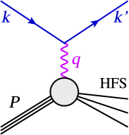
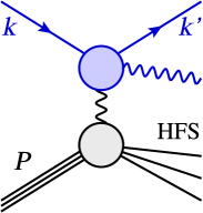
Figure 1: Illustration of $ep$ scattering. Left: (QED) Born-level diagram. Middle: generic illustration of a radiative leptonic tensor including higher-order QED corrections at the lepton vertex (the box-diagrams are additive and not shown). Right: practical implementation of QED higher-order corrections in MC event generators in terms of initial state radiation (ISR, green), final state radiation (FSR, red), and an effective coupling (orange).

Due to azimuthal symmetry and ignoring mass effects, only two variables of the outgoing four-vectors are of relevance. The usual choice is

• the scattered electron energy $E$ and its polar angle $\theta$, and

• the energy-momentum balance of the HFS, $\Sigma=E_{h}-p_{z,h}$, and the inclusive angle of the HFS $\gamma$.

The HFS quantity $\Sigma$ can be calculated as the sum of all HFS particles $\Sigma=\textstyle{\sum_{i}^{\text{HFS}}}(E_{i}-p_{z,i})$, and $\gamma$ is defined using the transverse momentum of the HFS, $T$, through $\tan\frac{\gamma}{2}=\frac{\Sigma}{T}$. Together with the electron-beam energy $E_{0}$, five observables are known, while three of them suffice to define a basic reconstruction method for $Q^{2}$, $y$ and $x$. Only for $x$ one further needs the proton beam energy $E_{p}$.

Table 1 summarizes some of the most common reconstruction methods, which use derived quantities from the scattered electron and HFS including $p_{T,e}^{2}=E^{2}\sin^{2}\theta$, $p_{z,e}=E\cos\theta$, $\Sigma_{e}=E-p_{z,e}=E(1-\cos\theta)$, $\tan\frac{\theta}{2}=\frac{\Sigma_{e}}{p_{T,e}}$ and $T^{2}=p_{x,h}^{2}+p_{y,h}^{2}=(\textstyle{\sum_{i}^{\text{HFS}}}p_{x,i})^{2}+(\textstyle{\sum_{i}^{\text{HFS}}}p_{y,i})^{2}=E^{2}_{h}\sin^{2}\gamma=\Sigma^{2}\cot^{2}\frac{\gamma}{2}=\Sigma(2E_{h}-\Sigma)$.

Method name	Observables	$y$	$Q^{2}$	$x\cdot E_{p}$
Electron ($e$)	$[E_{0}$,$E$,$\theta]$	$1-\frac{\Sigma_{e}}{2E_{0}}$	$\frac{E^{2}\sin^{2}\theta}{1-y}$	$\frac{E(1+\cos\theta)}{2y}$
Double angle (DA) Hoeger:1991wj ; Bentvelsen:1992fu	$[E_{0}$,$\theta$,$\gamma]$	$\frac{\tan\tfrac{\gamma}{2}}{\tan\tfrac{\gamma}{2}+\tan\tfrac{\theta}{2}}$	$4E_{0}^{2}\cot^{2}\tfrac{\theta}{2}(1-y)$	$\frac{Q^{2}}{4E_{0}y}$
Hadron ($h$, JB) JB:1979	$[E_{0}$,$\Sigma$,$\gamma]$	$\frac{\Sigma}{2E_{0}}$	$\frac{T^{2}}{1-y}$	$\frac{Q^{2}}{2\Sigma}$
ISigma (I$\Sigma$) Bassler:1994uq	$[E$,$\theta$,$\Sigma]$	$\frac{\Sigma}{\Sigma+\Sigma_{e}}$	$\frac{E^{2}\sin^{2}\theta}{1-y}$	$\frac{E(1+\cos\theta)}{2y}$
IDA Bentvelsen:1992fu	$[E$,$\theta$,$\gamma]$	$y_{\text{DA}}$	$\frac{E^{2}\sin^{2}\theta}{1-y}$	$\frac{E(1+\cos\theta)}{2y}$
$E_{0}E\Sigma$	$[E_{0}$,$E$,$\Sigma]$	$y_{h}$	$4E_{0}E-4E_{0}^{2}(1-y)$	$\frac{Q^{2}}{2\Sigma}$
$E_{0}\theta\Sigma$	$[E_{0}$,$\theta$,$\Sigma]$	$y_{h}$	$4E_{0}^{2}\cot^{2}\tfrac{\theta}{2}(1-y)$	$\frac{Q^{2}}{2\Sigma}$
$\theta\Sigma\gamma$ Bassler:H1intnote93	$[\theta$,$\Sigma$,$\gamma]$	$y_{\text{DA}}$	$\frac{T^{2}}{1-y}$	$\frac{Q^{2}}{2\Sigma}$
Double energy (A4) Bentvelsen:1992fu	$[E_{0}$,$E$,$E_{h}]$	$\frac{E-E_{0}}{(xE_{p})-E_{0}}$	$4E_{0}y(xE_{p})$	$E+E_{h}-E_{0}$
$E\Sigma T$	$[E$,$\Sigma$,$T]$	$\frac{\Sigma}{\Sigma+E\pm\sqrt{E^{2}+T^{2}}}$	$\frac{T^{2}}{1-y}$	$\frac{Q^{2}}{2\Sigma}$
$E_{0}ET$	$[E_{0}$,$E$,$T]$	$\frac{2E_{0}-E\mp\sqrt{E^{2}-T^{2}}}{2E_{0}}$	$\frac{T^{2}}{1-y}$	$\frac{Q^{2}}{4E_{0}y}$
Sigma ($\Sigma$) Bassler:1994uq	$[E_{0}$,$E$,$\Sigma$,$\theta]$	$y_{\text{I}\Sigma}$	$Q^{2}_{\text{I}\Sigma}$	$\frac{Q^{2}}{4E_{0}y}$
$e$Sigma ($e\Sigma$) Bassler:1994uq	$[E_{0}$,$E$,$\Sigma$,$\theta]$	$\frac{2E_{0}\Sigma}{(\Sigma+\Sigma_{e})^{2}}$	$2E_{0}E(1+\cos\theta)$	$\frac{E(1+\cos\theta)(\Sigma+\Sigma_{e})}{2\Sigma}$

Table 1: Summary of basic reconstruction methods that employ only three out of five quantities: $E_{0}$ (electron-beam energy), $E$ and $\theta$ (scattered electron energy and polar angle), $\Sigma$ and $\gamma$ (longitudinal energy-momentum balance, $\Sigma=\textstyle\sum_{\text{HFS}}(E_{i}-p_{z,i})$, and the inclusive angle of the HFS). Alternatively, the A4 method makes use of the HFS total energy $E_{h}$. Shorthand notations are used for the longitudinal energy-momentum balance of the electron, $\Sigma_{e}$, and for the transverse momentum of the HFS, $T$. The $E\Sigma T$ and $E_{0}ET$ methods are under-constrained and have two solutions, referring to two possible electron polar angles, and several more are existent when using $E_{h}$ (see Ref. Bentvelsen:1992fu for two examples). The two bottom rows provide the equations of the $\Sigma$ and $e\Sigma$-methods, which combine quantities of different basic reconstruction methods, while further methods (like the PT (rD$\Sigma$), D$\Sigma$, r$e\Sigma$ or mixed method) are found, e.g., in Ref. Bassler:1994uq ; Bassler:1997tv .

Each of these methods has pros and cons, and yield good performance in limited kinematic ranges Bentvelsen:1992fu ; Bassler:1994uq ; Bassler:1997tv . For example, the methods that mostly rely on the scattered electron yield the best resolution in events with large $y$, but their resolution on $x$ quickly diverges at low $y$. In contrast, the methods that rely mostly on the HFS variables yield better performance at low $y$, but are rather limited at high $y$. Consequently, the H1 and ZEUS collaborations have used different methods in different kinematic ranges (see Refs. Klein:2008di ; H1:2015ubc and references therein). For example, in Refs. H1:2009bcq ; H1:2012qti ; H1:2013ktq , the electron method is used for $y\gtrsim 0.19$, while the $\Sigma$ or $e\Sigma$ method are used at lower $y$, and DA method is employed for calibration.

In a massless, Born-level calculation, all methods yield equivalent results because of momentum and energy conservation ($2E_{0}=\Sigma+\Sigma_{e}$, $p_{T,e}=T$ and $Q^{2}=sxy$). However, once (real) higher-order QED effects are considered, the various methods yield different results and the calculated quantities for $Q^{2}$, $y$ and $x$ are not representative for the $\gamma/Z+p$ scattering process at the hadronic vertex.

Higher-order QED effects at the lepton vertex are generically represented as a correction to the leptonic tensor, as displayed in the middle diagram of Figure 1. Such radiative corrections include QED bremsstrahlung off the lepton, photonic lepton-vertex corrections, self-energy contributions at the external lepton lines, and fermionic contributions to the running of the fine-structure constant, and additional box-diagrams representing multi-boson exchange. The complete first-order corrections are calculable semi-analytically Spiesberger:237380 ; Kwiatkowski:1990cx ; Kwiatkowski:1990es ; Blumlein:1994ii ; Arbuzov:1995id . For an implementation in Monte-Carlo (MC) event generators, these calculations are split by partial-fraction decomposition into initial-state and final-state photon radiation (ISR and FSR) and using effective couplings, as displayed in the right diagram of Figure 1.

Two techniques are commonly applied to reduce sensitivity to QED radiation. The first technique is to merge the FSR photons with the electron, thus providing the four-vector linked to the exchanged boson, and the second technique is to take the ISR radiation to be collinear, which implies that $(\Sigma+\Sigma_{e})/2$ provides the incoming electron beam energy that contributes in the interaction. For soft and collinear FSR, the first is done implicitly also at detector level, e.g. when the photon is measured in the same calorimeter cell as the electron. ISR photons often escape undetected through the beam hole of the detector.

In cross-section measurements, the radiative particle-level is commonly just an intermediate step, and additionally requires the application of well-defined QED correction factors. For precision measurements, these factors should be small. Common definitions for cross sections in DIS are:

• Structure-function measurements are made as a function of $Q^{2}$ and $x$ and are quoted at the ‘Born-level’ and thus have to correct for all higher-order QED effects, such that the fine-structure constant factorizes from the calculation of the structure functions.

• At HERA, measurements of the HFS were quoted as non-radiative $\gamma^{*}p$ cross sections, which are corrected for first-order QED and electroweak effects.

A radiative cross section can be defined by merging any radiated photon with the scattered electron that is closer to the scattered electron than to the electron beam. By specifying a single reconstruction method, a well-defined, meaningful and almost model-independent definition of $Q^{2}$, $y$ and $x$ is obtained.

In the following, we will deal carefully with radiated photons at the particle level and the detector level to determine kinematic quantities $Q^{2}$, $y$ and $x$, in an optimal way. These observables can then be used for subsequent cross-section measurement with small and well-defined QED corrections.

3 Method

We use TensorFlow tensorflow to construct and train a DNN to estimate the DIS kinematics using both the scattered electron and the HFS. To demonstrate our methodology, we use a fast simulation of the proposed EIC experiment ATHENA using the Delphes package deFavereau:2013fsa ; miguel_arratia_2021_4592887 . After presenting results for ATHENA, we will show results applying the same methodology to a full simulation of the H1 experiment Brun:1987ma ; H1:1996prr ; H1:1996jzy . Both studies use the Rapgap MC generator Jung:1993gf , which employs routines from Refs. Bengtsson:1987kr ; Bentvelsen:1992fu ; Ingelman:1996mq ; Dobbs:2001ck . For H1, Rapgap version 3.1 is used, while verion 3.3 is used for the ATHENA studies. In addition, the MC generator Djangoh 1.4 Charchula:1994kf is used to test prior dependence. Both MC generators employ the Heracles routines Spiesberger:237380 ; Kwiatkowski:1990cx ; Kwiatkowski:1990es for the simulation of higher-order QED effects.

We restrict our study to events with $Q^{2}>200$ $\mathrm{GeV}^{2}$. This kinematic region is well measured, since the electron is scattered into the central regions of the detector. However, no single reconstruction method gives optimal performance over the full phase space Bassler:1994uq .

3.1 Fast simulation of the ATHENA experiment

Neutral-current DIS events are generated with the Rapgap 3.3 event generator for electron-proton scattering with beam energies of $E_{0}=18\,\mathrm{GeV}$ and $E_{p}=275\,\mathrm{GeV}$ and processed with the Delphes fast simulation of the ATHENA detector at the EIC. The scattered electron is selected as the highest-$p_{T}$ track that satisfies the following criteria: correct charge, $p_{T}>5$ GeV, electromagnetic fraction in the calorimeter $>0.80$, and isolation $<0.20$, where isolation is defined as the scalar $p_{T}$ sum of all other tracks and neutral hadrons within a cone of $\Delta R<0.5$ around the electron direction divided by the electron $p_{T}$. The HFS is reconstructed from the sum of all Energy-Flow candidates (tracks, photons, and neutral hadrons), excluding the scattered electron and any photon candidates that is within a cone of $\Delta R<0.4$ around the scattered electron. We require $\Sigma+\Sigma_{e}$ to be within $\pm 4\,\mathrm{GeV}$ of $2E_{0}$ to suppress ISR events.

3.2 QED radiation and categorization of events

We introduce a practical categorization of events, which is closely related to our proposed radiative cross-section definition above:

• if the radiated photon is closer to the electron-beam direction, it is an Initial-State Radiation event (ISR);

• if the radiated photon is closer to the scattered-electron direction, it is a Final-State Radiation event (FSR);

• if no photon radiation is emitted by the generator, it is a non-radiative event (NoR).

Within Rapgap, which implements first-order QED corrections, the radiated photon either branches off from the beam electron before it interacts with the proton, or it branches off of the scattered electron after interacting with the proton. This leads to the natural interpretation of the former as ISR and the latter as FSR, which agrees with our practical definitions in 94% of QED radiation events.

To define the target values of $Q^{2}$, $y$ and $x$ for events with QED radiation, we use the generated beam electron after radiation for ISR events and the generated scattered electron prior to radiation for FSR events. While this definition can be considered as the true kinematic quantities, alternative definitions in terms of particle-level observables are also possible. For example, by applying FSR merging and using the equations of ISR insensitive reconstructions methods for calculating $Q^{2}$, $y$ and $x$. In our studies, these different definitions yield indistinguishable results. The generator-level quantities are generically denoted with a subscript ‘gen’ in the following.

3.3 DNN inputs

For our main goal of determining $Q^{2}$, $y$ and $x$, the task of the DNN is in fact two-fold. In the absence of QED radiation, the task of the DNN would be to learn to compute $Q^{2}$, $y$ and $x$ from the input quantities subject to finite-resolution and acceptance effects. In events with QED radiation, the DNN needs to learn to quantify the extent of QED radiation and account for it while calculating $Q^{2}$, $y$ and $x$. Hence, the regression DNN must learn to treat ISR, FSR, and NoR events separately in order to achieve optimal performance. This is a key feature of our DNN method, which is absent in traditional methods.

We define the following variables to characterize the strength of QED radiation in the event:

$$p_{T}^{\rm bal}\ =\ 1-\frac{p_{T,e}}{T}\ =\ 1-\frac{\Sigma_{e}\tan\frac{\gamma}{2}}{\Sigma\tan\frac{\theta}{2}}\ \ \ ~{}~{}\text{and}~{}~{}\ \ \ p_{z}^{\rm bal}\ =\ 1-\frac{\Sigma_{e}+\Sigma}{2\ E_{0}}\,.$$ (2)

When calculating them at particle level, both quantities $p_{T}^{\rm bal}$ and $p_{z}^{\rm bal}$, are zero for events with no QED radiation, but positive for events with FSR and ISR, respectively. The $p_{T}^{\rm bal}$ ($p_{z}^{\rm bal}$ ) value indicates the strength of FSR (ISR).

The following observables that help indicate QED radiation in the event are included as inputs to the regression DNN for $Q^{2}$, $y$ and $x$:

• The values of $p_{T}^{\rm bal}$ and $p_{z}^{\rm bal}$.

• The energy, $\eta$, and $\Delta\phi$ of the reconstructed photon in the event that is closest to the electron-beam direction, where $\Delta\phi$ is with respect to the scattered electron.

• The sum ECAL energy within a cone of $\Delta R<0.4$ around the scattered electron divided by the scattered-electron track momentum.

• The number of ECAL clusters within a cone of $\Delta R<0.4$ around the scattered electron.

These seven observables are combined with the following eight:

• Scattered-electron quantities $p_{T,e}$, $p_{z,e}$ and $E$.

• HFS four-vector quantities $T$, $p_{z,h}$ and $E_{h}$.

• $\Delta\phi(e,h)$ between the scattered electron and the HFS momentum vector.

• The difference $\Sigma_{e}-\Sigma$.

The transverse momenta of the scattered electron and the HFS are highly correlated. We replace the pair of $p_{T}$ values with the difference and the sum of the $p_{T}$ values, which removes the correlation and aids the DNN training. The sum $\Sigma_{e}+\Sigma$ appears in the definition of $p_{z}^{\rm bal}$ and is sharply peaked at twice the electron-beam energy, making the $\Sigma$ values anti-correlated; hence, we include the orthogonal combination $\Sigma_{e}-\Sigma$ in addition.

3.4 DNNs for the classification or quantification of QED radiation

To determine the ability of the DNN to identify and quantify QED radiation, we investigated two approaches: a classification network and a regression network for $p_{T}^{\rm bal}$ and $p_{z}^{\rm bal}$. Both DNNs differ only in the activation function for the final layer, the learning targets, and the loss function for the training.

We followed a heuristic approach in designing the DNN, guided by prior experience. We chose to have the number of nodes per hidden layer grow in the first layers, reach a peak size, and then fall at a rate that is symmetric about the peak layer. Several trial configurations were tested, each with a different number of hidden layers and/or number of nodes per layer, though we did not perform a thorough scan. We also tried a few sets of optimizer hyperparameters before finding values that gave good results in a reasonable amount of training time. Various standard activation functions were tested with no appreciable differences in the results. This basic DNN design is effective for a variety of tasks, including classification and regression, as we explain below. The same design works well for both the ATHENA fast simulation and the H1 full simulation. Our design explorations were terminated once we achieved DIS reconstruction performance that exceeded the conventional methods. We have not carried out thorough hyperparameter scans, so further improvements may be possible.

The QED-classification DNN consists of a sequential network with 8 layers. The 15 DNN inputs, defined in the previous section, are transformed prior to training to have zero mean and unit RMS using the sklearn StandardScaler scikit-learn . The learning targets are three binary (0 or 1) state variables to tag the events as ISR, FSR, or NoR. The activation function is a rectified linear unit (relu) for the first layer, scaled exponential linear unit (selu) NIPS2017_5d44ee6f for the middle layers, and the softmax function for the final output layer. The numbers of nodes per layer are 64, 128, 512, 1024, 512, 128, and 64, with 3 outputs in the final layer. The outputs are three numbers, each between 0 and 1, that sum up to 1. The loss function for the training is categorical cross entropy. The training is performed with the Adam optimizer kingma2017adam with a learning rate of $10^{-4}$. The total number of parameters of the DNN model is 1,199,555. The training and validation are performed using over 28 million simulated events with half for training and half for validation. The batch size for the training is 128. The training terminates after 38 epochs, finding no further improvement in the validation loss function.

Figure 2 shows distributions for the three outputs of the QED-classification DNN. Some events have clear evidence of QED radiation and are strongly identified. Some degree of mis-classification is to be expected, since neither soft ISR/FSR, nor collinear FSR induce a measurable signal in the detector.

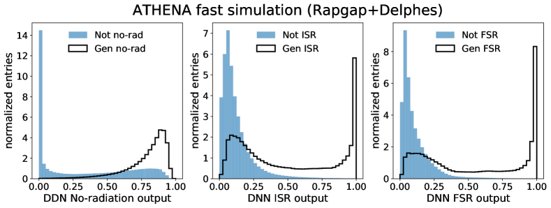
Figure 2: Distributions of the QED-classification DNN predictions for the ATHENA fast simulation. The distributions are normalized to equal area.

In the second study, the QED regression for $p_{T}^{\rm bal}$ and $p_{z}^{\rm bal}$, the DNN has the same structure as the QED-classification DNN except for the following differences. The activation function is the linear function for the final output layer, which has 2 nodes instead of 3. The learning targets are the particle-level values of $p_{T}^{\rm bal}$ and $p_{z}^{\rm bal}$, which are transformed to have zero mean and unit RMS prior to training. The loss function for the training is Huber loss 10.1214/aoms/1177703732 with a transition between quadratic and linear loss at $\pm 0.01$. The batch size for the training is 1024. The training and validation are done using the same sample as for the QED-classification DNN.

Figure 3 shows distributions of the DNN predictions for $p_{T}^{\rm bal}$ and $p_{z}^{\rm bal}$, separately for ISR, FSR, and NoR events, as well as scatter plots of the predicted values vs the particle-level values. The predicted $p_{T}^{\rm bal}$ distribution for FSR events is shifted to positive values for FSR events, while the predicted $p_{z}^{\rm bal}$ distribution is shifted to positive values for ISR events, as expected. For many events, the DNN is able to accurately estimate both $p_{T}^{\rm bal}$ and $p_{z}^{\rm bal}$. There are also QED-radiation events where the prediction is zero, which correspond to cases where the radiated photon is either out of acceptance or not clearly identified.

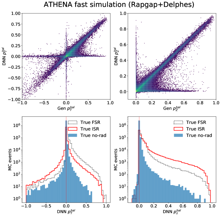
Figure 3: Distributions of the QED-regression DNN predictions and particle-level values of $p_{T}^{\rm bal}$ and $p_{z}^{\rm bal}$ for the ATHENA fast simulation.

3.5 Regression DNN for DIS kinematic variables $Q^{2}$, $y$ and $x$

We estimate $Q^{2}$, $y$ and $x$ using a regression DNN that has a similar structure as the QED regression DNN described above, except for the final output layer that has three nodes corresponding to the target variables $Q^{2}$, $y$ and $x$. The learning rate is $10^{-5}$ and the batch size is 1024. Since the distributions of $Q^{2}$, $y$ and $x$ are approximately exponential, the DNN is trained to predict the logarithm of each variable. The training and validation are performed using over 28 million events, using half for validation and half for training.

As a pilot study, we consider three different choices for the input variables to the DNN:

• add the three QED-classification DNN outputs (FSR, ISR, NoR) as inputs, in addition to the 15 variables.

• add the QED-regression DNN predictions $p_{T}^{\rm bal}$ and $p_{z}^{\rm bal}$ as inputs, in addition to the 15 variables.

• use the same 15 inputs as in the QED-classification and regression DNNs.

We found that the results of these three approaches are essentially the same. This suggests that the QED-classification and the QED-regression DNNs do not provide any additional information beyond what the regression DNN for $Q^{2}$, $y$ and $x$ learned. In light of this, we chose the simplest (third) option, which uses only the original 15 variables as inputs. The total number of parameters for the DNN model is 1,199,619. The training terminates after 103 epochs, finding no further improvement in the validation loss function.

3.6 Benchmark of the DNN reconstruction vs. standard methods

Figure 4 shows the results for the DNN and traditional methods using events with $Q^{2}>200~{}{\rm GeV}^{2}$ and two $y$ regions, obtained with the ATHENA fast simulation.

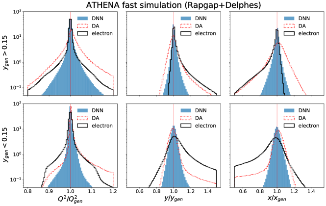
Figure 4: Resolution for $Q^{2}$ (left), $y$ (middle), and $x$ (right) for the DNN, electron, and double-angle (DA) methods for the fast simulation of the ATHENA experiment. The top (bottom) row is for events with $y_{\rm gen}>0.15$ ($y_{\rm gen}<0.15$). All distributions are normalized to the same area.

The resolutions from the DNN exhibit a peak at unity and mostly Gaussian-like tails; in contrast, classical methods yield a peak but larger tails caused by their limited use of the reconstructed quantities and the presence of ISR or FSR.

ATHENA fast simulation (Rapgap+Delphes)

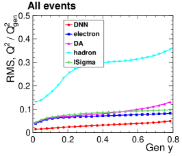
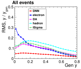
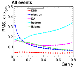
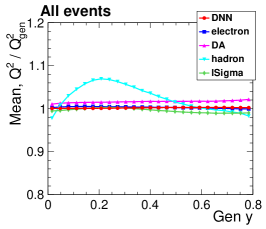
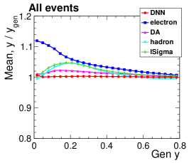
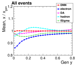
Figure 5: Resolution on the reconstruction of $Q^{2}$ (left), $y$ (middle), and $x$ (right) as a function of the generated $y$ for the fast simulation of ATHENA. The top (bottom) row shows the RMS (mean) of the measured-over-generated distribution as a function of generated $y_{\text{gen}}$. The RMS and mean are calculated using events with the measured-over-generated ratio within the interval 0 to 2.

The properties of the resolutions, their mean and RMS, are displayed in Figure 5 for small intervals of $y$ . The DNN reconstruction has the smallest RMS among all methods, for all three kinematic variables and all $y$ intervals. Also, the mean distributions are unbiased for $Q^{2}$, $y$ and $x$ for all $y$ intervals, while the classical methods exhibit large biases.

We examine more closely the resolution and bias for events with and without QED radiation in Figures 6 and 7, where we use the definition of NoR, ISR and FSR events from Section 3.2. The RMS for events with no QED radiation gives a measure of the core resolution, free from the tails that are visible in the distributions of Figure 4 for the conventional methods. All methods, except the hadron method, show no bias in NoR events. For $x$ and $y$, the electron method has a better core resolution than the DNN for $y>0.15$; however, it suffers from poorer resolution and a strong bias in events with QED radiation. The DNN reconstruction has some loss in performance in QED-radiation events, but it is about a factor of two better than the electron method in these events, and shows no bias. We conclude that the DNN has successfully learned to mitigate the effects of QED radiation that spoil the resolution and bias the calculations of the conventional methods.

ATHENA fast simulation (Rapgap+Delphes)

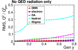
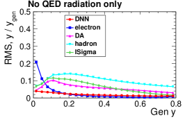
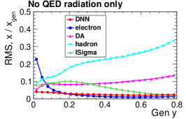
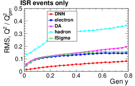
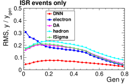
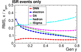
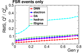
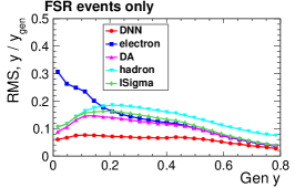
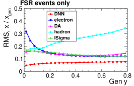
Figure 6: Comparison of the RMS of the resolution of $Q^{2}$, $y$ and $x$ (from left to right) for NoR (top), ISR (middle), and FSR (bottom) events. The RMS is calculated using events with the measured-over-generated ratio within the interval 0 to 2.

ATHENA fast simulation (Rapgap+Delphes)

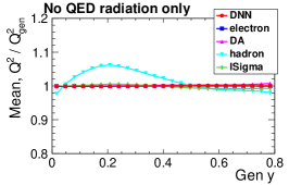
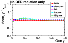
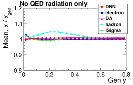
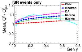
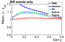
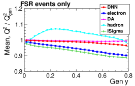
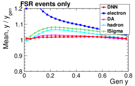
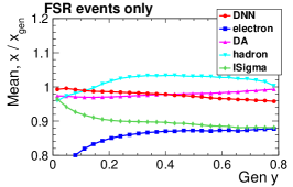
Figure 7: Comparison of the mean of the resolution distributions of $Q^{2}$, $y$ and $x$ (from left to right) for NoR (top), ISR (middle), and FSR (bottom) events. The mean is calculated using events with the measured-over-generated ratio within the interval 0 to 2.

4 Demonstration using the full simulation of the H1 experiment

We apply our DNN methodology to simulated events of the H1 experiment at HERA. The events were simulated by the H1 Collaboration using the Rapgap 3.1 Jung:1993gf and Djangoh 1.4 Charchula:1994kf generators for the beam energies $E_{0}=27.6\,\mathrm{GeV}$ and $E_{p}=920\,\mathrm{GeV}$. The generators employ the Heracles routines Spiesberger:237380 ; Kwiatkowski:1990cx ; Kwiatkowski:1990es for QED radiation, the CTEQ6L PDF set Pumplin:2002vw , and the Lund hadronization model Andersson:1983ia with parameters fitted by the ALEPH Collaboration Schael:2004ux . The simulation of the H1 experiment H1:1996prr ; H1:1996jzy employs the Geant 3 package Brun:1987ma and includes real calorimeter noise and fast shower simulations Fesefeldt:1985yw ; Grindhammer:1989zg ; Gayler:1991cr ; Kuhlen:1992ey ; Grindhammer:1993kw ; Glazov:2010zza . The simulation includes time-dependent properties (‘run-specific’), where the detector state and beam properties correspond altogether to the HERA-II data taking periods.

The simulated events are reconstructed just like data, in particular, an energy-flow algorithm energyflowthesis ; energyflowthesis2 ; energyflowthesis3 is used to define objects whose sum yields the HFS four-vector, and the scattered electron candidate are defined using the same approach as Refs. H1:2012qti ; Andreev:2014wwa ; H1:2021wkz . The simulated events also undergo the same (in-situ) calibration procedure as real data, using the latest calibration by the H1 Collaboration H1:2012qti ; Kogler:2011zz ; Andreev:2014wwa . Some technical selections and fiducial cuts are applied as it would be done similarly to real data. In particular, events are required to have $45<\Sigma+\Sigma_{e}<65$ GeV to suppress ISR events; a veto on QED Compton events is imposed; and since a trigger simulation is included, our study is limited to $E\gtrsim 11\,\mathrm{GeV}$ Andreev:2014wwa . The simulated events are processed within H1’s computing environment Britzger:2021xcx and altogether several $10^{8}$ events were simulated, and after ‘run’-selection, acceptance effects and our selection of $Q^{2}>200\,\mathrm{GeV}^{2}$ yield about $7\cdot 10^{7}$ simulated and reconstructed events for our DNN studies.

We use the same regression DNN structure, input variables, and training methods for the simulated H1 events as previously for the ATHENA events. We take a sample of over 12 million Rapgap events and use half of the events for training and half for validation. The training terminates after 125 epochs, finding no further improvement in the validation loss function.

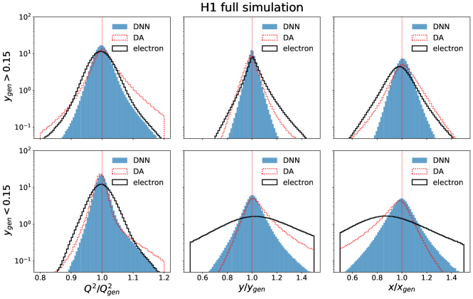
Figure 8: Resolution for $Q^{2}$ (left), $y$ (middle), and $x$ (right) for the DNN, electron, and double-angle (DA) reconstruction methods for the full simulation of the H1 experiment. The top (bottom) row is for events with $y_{\rm gen}>0.15$ ($y_{\rm gen}<0.15$). All distributions are normalized to the same area.

Figure 8 shows the resolutions for the DNN and two classical methods in two intervals of $y$. Similarly to the results obtained with the ATHENA simulation, the DNN yields a peak at unity and no asymmetric tails for all three quantities, in contrast with classical methods.

H1 full simulation

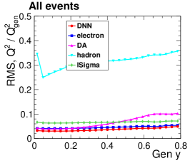
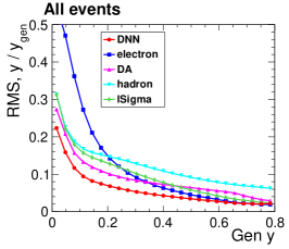
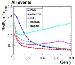
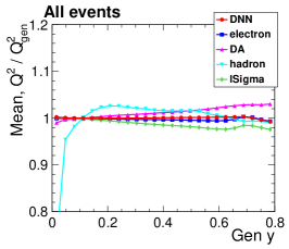
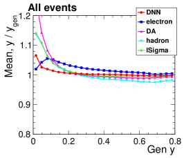
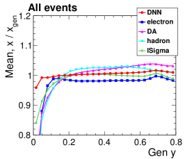
Figure 9: Resolution on the reconstruction of $Q^{2}$ (left), $y$ (middle), and $x$ (right) as a function of the generated $y$ for the full simulation of H1. The top (bottom) row shows the RMS (mean) of the measured-over-generated distribution as a function of the generated $y$. The RMS and mean are calculated using events with the measured-over-generated ratio within the interval 0 to 2.

The mean and RMS of the resolutions are displayed as a function of $y$ in Figure 9. The DNN yields the smallest RMS. The mean of the DNN reconstruction is closest to unity over a wide range of $y$. Only for $Q^{2}$, or at highest $y$, the electron method achieves comparably good RMS and mean. In contrast, at lower $y$ the DNN provides a significant improvement and results in a bias-free reconstruction of $y$ and $x$ with superior resolution.

To assess a possible bias in our DNN methodology that may arise from the details of the MC event generator that is used to train the DNN, we study the performance of the DNN reconstruction using two different MC event generators, Rapgap and Djangoh. The two event generators differ in the modelling of higher-order QCD radiation that results in significant differences in the prediction of the HFS. Djangoh employs the color-dipole model, while Rapgap employs a matrix-element plus parton shower model, where the parton shower is in the leading-logarithmic approximation. In this study, we use H1’s full simulation and train the DNN with a Rapgap event sample. Subsequently this DNN is applied to a statistically independent Rapgap event sample and to a simulated Djangoh sample.

Figure 10 shows the $Q^{2}$, $y$ and $x$ resolutions as a function of the generated $y$ for both the Rapgap and Djangoh samples when using the same DNN, where the measured-over-generated ratio is calculated on an event-by-event basis with the respective generated values. The results from the Djangoh event sample are nearly indistinguishable from the Rapgap sample. In particular, the mean of the distribution is unbiased. This result suggests that any generator-specific systematic errors in the DNN predictions is negligible.

H1 full simulation

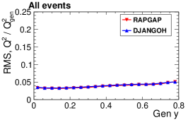
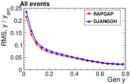
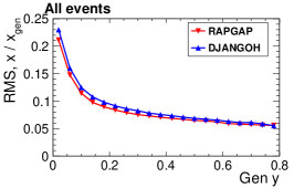
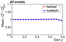
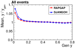
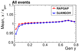
Figure 10: Resolution comparison of the Rapgap and Djangoh generators on the DNN reconstruction of $Q^{2}$ (left), $y$ (middle), and $x$ (right) as a function of the generated $y$ for the full simulation of H1. The top (bottom) row shows the RMS (mean) of the measured-over-generated distribution as a function of the generated $y$. The red (blue) curves show the results for the Rapgap (Djangoh) event sample, while the DNN was trained with the Rapgap sample in both cases.

The resolution (RMS) for $y$ and $x$ increase at lower $y$, even for the DNN reconstruction. Since this pattern is not present in the the ATHENA fast simulation results and may be attributed to further acceptance, noise, or resolution effects that deteriorates the measurement of the HFS energyflow . A dedicated study using a Delphes fast simulation is presented in the following section.

5 Impact of further acceptance and resolution effects at low $y$

At low $y$, the HFS-based methods perform better than the electron method. The reason is, that the ratio $E(1-\cos\theta)/2E_{0}$ gets close to one and cannot be measured accurately because of large values of $E$. Likewise, however, the HFS momentum balance $\Sigma$ goes to zero as $y$ goes to zero. Although for kinematic reconstruction at low $y$ the usage of $\Sigma$ is preferred over $\Sigma_{e}$, the quantity $\Sigma$ is particularly sensitive to resolution and acceptance effects. In particular HFS components that are more in the central region of the calorimeter contribute more, such making $\Sigma$ at low $y$ especially sensitive resolution effects or efficiency losses in the central part of the detector or fake components from calorimetric noise.

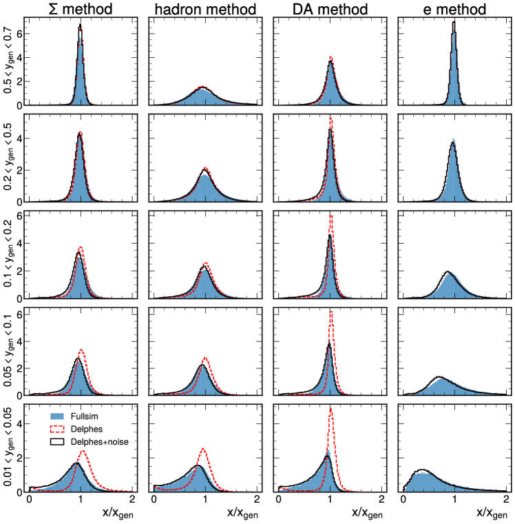
Figure 11: Resolutions for $x$ in various $y$ ranges and reconstruction methods obtained with a full Geant simulation of H1 (shaded area) and a fast simulation based on Delphes with (full line) and without (dashed line) an added ad-hoc noise contribution.

The Delphes fast simulation does not include calorimeter noise hits, nor does it account in a full-fledged manner for single-particle acceptance effects and efficiency losses as they can be present at the boundaries of calorimeter stacks or because of insensitive material. To test the hypothesis that such detector effects can be responsible for the resolution decrease in $x$ and $y$ for hadronic reconstruction methods at low $y$ ($y\lesssim 0.15$), we have implemented the H1 experiment in Delphes. Figure 11 shows the $x$ resolution for the standard reconstruction methods for our fast simulation of H1 compared to the full simulation. The agreement between the fast and full simulation at high $y$ is fairly good. At low $y$, however, there is a low-side tail for the $\Sigma$, hadron and DA method for events processed with the full H1 simulation, while that tail is absent in the fast simulation, and also the mean value is shifted.

We apply an additional additive component with random sign to the HFS to the fast simulated events, which mimics further detector effects, like acceptance or efficiency losses, reduced resolution or artificial components from electronic noise in the calorimeter. The model we use to simulate these effects is to generate random numbers from TRandom::Landau in Root citeulike:363715 with mu=0 and sigma=0.05 in units of GeV, and add it with a random sign to the $p_{x}$, $p_{y}$, and $p_{z}$ components of the reconstructed HFS four-vector.

The results are also displayed in Figure 11. We find that adding such an additional detector effect to the HFS in the fast simulation brings the fast simulation into good agreement with the full detector simulation. Adding these ad-hoc detector effects produces a low-side tail in the $x$ resolution at low $y$ but does not affect the $x$ reconstruction at high $y$. The electron remains naturally unaltered in that procedure.

This study suggests that further detector effects that are otherwise not included in the Delphes fast simulation impact the precise measurement of the HFS and reduce the $x$ and $y$ resolution at low $y$. We do not currently have an estimate for how large that effect in ATHENA will be, what is the actual correspondence in the full simulation (an acceptance, efficiency, resolution or noise effect), or to which extent it is impacted by calibration or noise-suppression algorithms. Though, due to a larger coverage of the calorimeter, less dead material and newer detector technologies of ATHENA as compared to H1, we expect this additive component to be significantly smaller for ATHENA than what our ad-hoc model adds to H1 to bring the fast and full simulation into agreement.

To place an upper bound on the impact of these effects in the ATHENA results, we investigated adding our ad-hoc component to the ATHENA fast simulation. The full analysis is then repeated, including the DNN training. The results are shown in Figure 12 for both the conventional reconstruction methods and the DNN reconstruction, where the DNN reconstruction for the unaltered ATHENA sample is included for comparison. The DNN resolution does get worse below $y$ of around 0.2 and there is a small bias at very low $y$, as we expected based on the H1 study. The $Q^{2}$ reconstruction is insensitive to that, since it is dominated by the electron reconstruction. The results in Figure 12 show that also with a very conservative ad-hoc model, the DNN outperforms all standard reconstruction methods.

ATHENA fast simulation with additive resolution effect (Rapgap+Delphes)

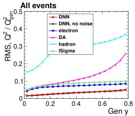
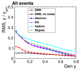
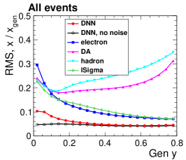
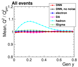
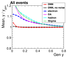
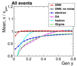
Figure 12: Resolution on the reconstruction of $Q^{2}$ (left), $y$ (middle), and $x$ (right) as a function of the generated $y$ for the fast simulation of ATHENA with the ad-hoc additive resolution effects model added. The top (bottom) row shows the RMS (mean) of the measured-over-generated distribution as a function of the generated $y$. For comparison, the DNN curves for that unaltered sample are shown in black for comparison.

6 Summary and outlook

We have presented a novel method to reconstruct the DIS kinematic variables ($Q^{2}$, $y$ and $x$) using a deep neural network (DNN) that takes as input the electron and hadronic-final-state measurements as well as observables that can indicate the presence of QED radiation.

We have introduced our methodology using a Delphes-based fast simulation of the ATHENA experiment for the EIC and validated our methods using the well-understood full simulation of the H1 experiment at HERA.

Our method outperforms traditional methods over a wide kinematic range, improving the resolution, and decreasing the bias. We validated that our method is independent of the Monte Carlo event generator used to train the DNN. We further performed a study to validate the fast simulation approach by comparing a Delphes model of the H1 detector with the H1 full simulation; these comparisons allowed us to identify key effects for low $y$ events.

Our DNN-based method shows promise for improving the resolution and extending the kinematic reach of flagship EIC measurements. Given that EIC experiments are being designed, our method offers a way to benchmark detector performance against DIS using an optimal combination of electron and HFS measurements.

Code availability

The code in this work can be found in: https://github.com/owen234/DIS-reco-paper/

Appendix A Detailed resolution plots for the ATHENA fast simulation

In this section detailed resolution plots for the variables $Q^{2}$ (Figure 13), $y$ (Figure 14) and $x$ (Figure 15) for the ATHENA fast simulation at the EIC with $\sqrt{s}=141\,\mathrm{GeV}$ are shown. Our DNN-reconstruction method is compared to four widely used basic reconstruction methods (I$\Sigma$, hadron, double-angle and electron-method) for $Q^{2}>200\,\mathrm{GeV}^{2}$ in five kinematic ranges in $y_{\text{gen}}$.

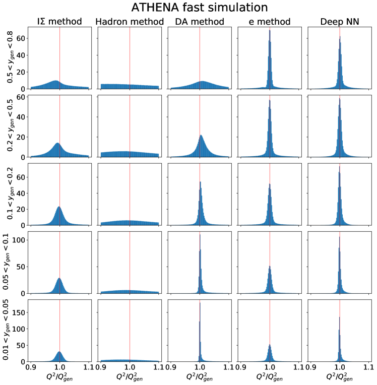
Figure 13: Resolutions for $Q^{2}$ in various $y$ ranges and reconstruction methods from the Delphes fast simulation of ATHENA for events with $Q^{2}>200~{}{\rm GeV}^{2}$. The tails in the distributions are from events with ISR and FSR radiation.

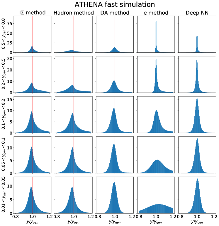
Figure 14: Resolutions for $y$ in various $y$ ranges and reconstruction methods from the Delphes fast simulation of ATHENA for events with $Q^{2}>200~{}{\rm GeV}^{2}$. The tails in the distributions are from events with ISR and FSR radiation.

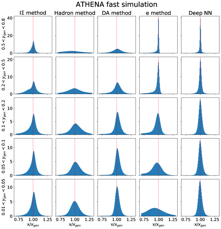
Figure 15: Resolutions for $x$ in various $y$ ranges and reconstruction methods from the Delphes fast simulation of ATHENA for events with $Q^{2}>200~{}{\rm GeV}^{2}$. The tails in the distributions are from events with ISR and FSR radiation.

Appendix B Detailed resolution plots for the H1 full simulation

In this section detailed resolution plots for the variables $Q^{2}$ (Figures 16 and 17), $y$ (Figure 18) and $x$ (Figures 19 and 20) for H1’s full simulation at HERA at $\sqrt{s}=319\,\mathrm{GeV}$ are shown. Our DNN-reconstruction method is compared to the full set of eight basic reconstruction methods (I$\Sigma$, hadron, double-angle (DA), electron ($e$), IDA, $E_{0}E\Sigma$, $E_{0}\theta\Sigma$, and $\theta\Sigma\gamma$-method) for $Q^{2}>200\,\mathrm{GeV}^{2}$ in five kinematic ranges in $y_{\text{gen}}$. The double-energy method is omitted since $E_{h}$ is not measureable du to relevant acceptance losses through the forward beam-hole. For $y$ there are only four unambiguous independent basic methods.

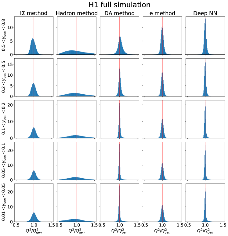
Figure 16: Resolutions for $Q^{2}$ in various $y$ ranges and reconstruction methods from the full simulation of H1 for events with $Q^{2}>200~{}{\rm GeV}^{2}$.

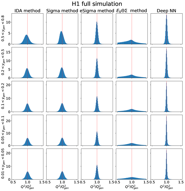
Figure 17: Resolutions for $Q^{2}$ in various $y$ ranges and reconstruction methods from the full simulation of H1 for events with $Q^{2}>200~{}{\rm GeV}^{2}$.

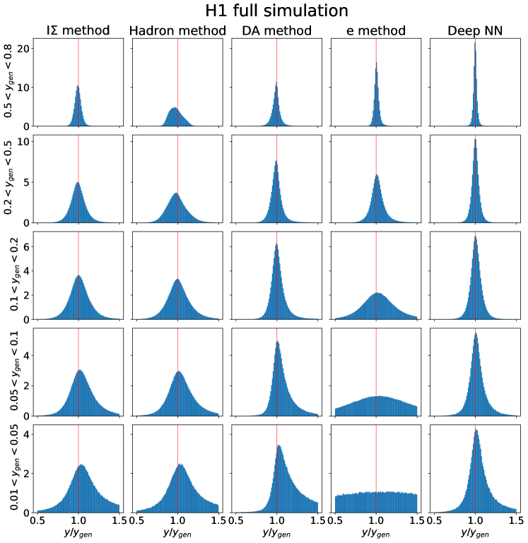
Figure 18: Resolutions for $y$ in various $y$ ranges and reconstruction methods from the full simulation of H1 for events with $Q^{2}>200~{}{\rm GeV}^{2}$.

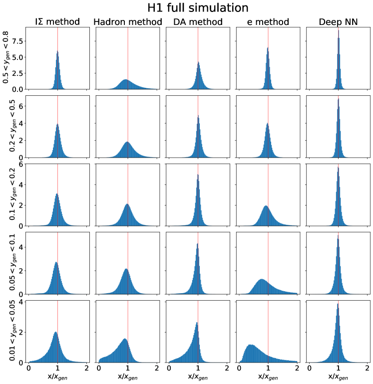
Figure 19: Resolutions for $x$ in various $y$ ranges and reconstruction methods from the full simulation of H1 for events with $Q^{2}>200~{}{\rm GeV}^{2}$.

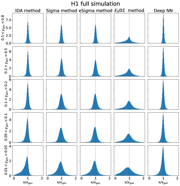
Figure 20: Resolutions for $x$ in various $y$ ranges and reconstruction methods from the full simulation of H1 for events with $Q^{2}>200~{}{\rm GeV}^{2}$.

References

- (1) R. K. Ellis, W. J. Stirling, B. R. Webber, QCD and Collider Physics, Cambridge University Press, 1996. doi:10.1017/CBO9780511628788.
- (2) R. Devenish, A. Cooper-Sarkar, Deep inelastic scattering, Oxford University Press, 2004. doi:10.1093/acprof:oso/9780198506713.001.0001.
- (3) P. A. Zyla, et al., Review of Particle Physics, PTEP 2020 (2020) 083C01. doi:10.1093/ptep/ptaa104.
- (4) A. Blondel, F. Jacquet, DETECTION AND STUDY OF THE CHARGED CURRENT EVENT , in: U. Amaldi, et al. (Eds.), Proceedings of the Study of an Facility for Europe, 1979, p. 391.
- (5) J. Blümlein, M. Klein, Kinematics and resolution at future colliders, in: 1990 DPF Summer Study on High-energy Physics: Research Directions for the Decade (Snowmass 90), 1990, pp. 549–551.
- (6) K. C. Hoeger, Measurement of , , in neutral current events, in: Workshop on Physics at HERA 1991, 1991.
- (7) S. Bentvelsen, J. Engelen, P. Kooijman, Reconstruction of () and extraction of structure functions in neutral current scattering at HERA, in: Workshop on Physics at HERA 1991, 1992.
- (8) U. Bassler, G. Bernardi, Progress on Kinematical Variables Reconstruction. Consequences for D.I.S. Physics Analysis at Low x, H1 internal note, H1-03/93-274 (Mar 1993).
- (9) U. Bassler, G. Bernardi, On the kinematic reconstruction of deep inelastic scattering at HERA: The Sigma method, Nucl. Instrum. Meth. A 361 (1995) 197–208. arXiv:hep-ex/9412004, doi:10.1016/0168-9002(95)00173-5.
- (10) M. Derrick, et al., Measurement of the F2 structure function in deep inelastic scattering using 1994 data from the ZEUS detector at HERA, Z. Phys. C 72 (1996) 399. arXiv:hep-ex/9607002, doi:10.1007/s002880050260.
- (11) U. Bassler, G. Bernardi, Structure function measurements and kinematic reconstruction at HERA, Nucl. Instrum. Meth. A 426 (1999) 583–598. arXiv:hep-ex/9801017, doi:10.1016/S0168-9002(99)00044-3.
- (12) A. Accardi, et al., Electron Ion Collider: The Next QCD Frontier: Understanding the glue that binds us all, Eur. Phys. J. A 52 (2016) 268. arXiv:1212.1701, doi:10.1140/epja/i2016-16268-9.
- (13) R. Abdul Khalek, et al., Science Requirements and Detector Concepts for the Electron-Ion Collider: EIC Yellow Report (Mar 2021). arXiv:2103.05419.
- (14) D. P. Anderle, et al., Electron-ion collider in China, Front. Phys. (Beijing) 16 (2021) 64701. arXiv:2102.09222, doi:10.1007/s11467-021-1062-0.
- (15) J. L. Abelleira Fernandez, et al., A Large Hadron Electron Collider at CERN: Report on the Physics and Design Concepts for Machine and Detector, J. Phys. G 39 (2012) 075001. arXiv:1206.2913, doi:10.1088/0954-3899/39/7/075001.
- (16) P. Agostini, et al., The Large Hadron-Electron Collider at the HL-LHC (Jul 2020). arXiv:2007.14491.
- (17) L. De Oliveira, B. Nachman, M. Paganini, Electromagnetic Showers Beyond Shower Shapes, Nucl. Instrum. Meth. A 951 (2020) 162879. arXiv:1806.05667, doi:10.1016/j.nima.2019.162879.
- (18) D. Belayneh, et al., Calorimetry with Deep Learning: Particle Simulation and Reconstruction for Collider Physics (Dec 2019). arXiv:1912.06794, doi:10.1140/epjc/s10052-020-8251-9.
-
(19)
ATLAS Collaboration, Deep
Learning for Pion Identification and Energy Calibration with the ATLAS
Detector, ATL-PHYS-PUB-2020-018 (2020).
URL http://cdsweb.cern.ch/record/2724632 - (20) P. Abratenko, et al., Convolutional neural network for multiple particle identification in the MicroBooNE liquid argon time projection chamber, Phys. Rev. D 103 (2021) 092003. arXiv:2010.08653, doi:10.1103/PhysRevD.103.092003.
- (21) A. Aurisano, A. Radovic, D. Rocco, A. Himmel, M. D. Messier, E. Niner, G. Pawloski, F. Psihas, A. Sousa, P. Vahle, A Convolutional Neural Network Neutrino Event Classifier, JINST 11 (2016) P09001. arXiv:1604.01444, doi:10.1088/1748-0221/11/09/P09001.
- (22) A. M. Sirunyan, et al., A Deep Neural Network for Simultaneous Estimation of b Jet Energy and Resolution, Comput. Softw. Big Sci. 4 (2020) 10. arXiv:1912.06046, doi:10.1007/s41781-020-00041-z.
-
(23)
Generalized Numerical Inversion: A
Neural Network Approach to Jet Calibration, Tech. Rep.
ATL-PHYS-PUB-2018-013, CERN, Geneva (Jul 2018).
URL http://cds.cern.ch/record/2630972 -
(24)
Simultaneous Jet Energy and Mass
Calibrations with Neural Networks, Tech. Rep. ATL-PHYS-PUB-2020-001, CERN,
Geneva (Jan 2020).
URL http://cds.cern.ch/record/2706189 - (25) P. Baldi, L. Blecher, A. Butter, J. Collado, J. N. Howard, F. Keilbach, T. Plehn, G. Kasieczka, D. Whiteson, How to GAN Higher Jet Resolution (Dec 2020). arXiv:2012.11944.
- (26) F. O. T. P. G. Kasieczka, M. Luchmann, Per-Object Systematics using Deep-Learned Calibration, SciPost Phys. 9 (2020) 089. arXiv:2003.11099, doi:10.21468/SciPostPhys.9.6.089.
- (27) S. Cheong and A. Cukierman and B. Nachman and M. Safdari and A. Schwartzman, Parametrizing the Detector Response with Neural Networks, JINST 15 (2020) P01030. arXiv:1910.03773, doi:10.1088/1748-0221/15/01/P01030.
- (28) L. de Oliveira, M. Kagan, L. Mackey, B. Nachman, A. Schwartzman, Jet-images — deep learning edition, JHEP 07 (2016) 069. arXiv:1511.05190, doi:10.1007/JHEP07(2016)069.
- (29) A. M. Sirunyan, et al., A deep neural network to search for new long-lived particles decaying to jets, Mach. Learn. Sci. Tech. 1 (2020) 035012. arXiv:1912.12238, doi:10.1088/2632-2153/ab9023.
- (30) M. Aaboud, et al., Performance of top-quark and -boson tagging with ATLAS in Run 2 of the LHC, Eur. Phys. J. C 79 (2019) 375. arXiv:1808.07858, doi:10.1140/epjc/s10052-019-6847-8.
- (31) A. Butter, et al., The Machine Learning Landscape of Top Taggers, SciPost Phys. 7 (2019) 014. arXiv:1902.09914, doi:10.21468/SciPostPhys.7.1.014.
- (32) A. Andreassen, P. T. Komiske, E. M. Metodiev, B. Nachman, J. Thaler, OmniFold: A Method to Simultaneously Unfold All Observables, Phys. Rev. Lett. 124 (2020) 182001. arXiv:1911.09107, doi:10.1103/PhysRevLett.124.182001.
- (33) K. Datta, D. Kar, D. Roy, Unfolding with Generative Adversarial Networks (2018). arXiv:1806.00433.
- (34) M. Bellagente, A. Butter, G. Kasieczka, T. Plehn, R. Winterhalder, How to GAN away Detector Effects, SciPost Phys. 8 (4) (2020) 070. arXiv:1912.00477, doi:10.21468/SciPostPhys.8.4.070.
- (35) A. Glazov, Machine learning as an instrument for data unfolding (Dec 2017). arXiv:1712.01814.
-
(36)
M. Vandegar, M. Kagan, A. Wehenkel, G. Louppe,
Neural Empirical
Bayes: Source Distribution Estimation and its Applications to
Simulation-Based Inference, in: A. Banerjee, K. Fukumizu (Eds.),
Proceedings of The 24th International Conference on Artificial Intelligence
and Statistics, Vol. 130 of Proceedings of Machine Learning Research, PMLR,
2021, pp. 2107–2115.
arXiv:2011.05836.
URL https://proceedings.mlr.press/v130/vandegar21a.html - (37) J. N. Howard, S. Mandt, D. Whiteson, Y. Yang, Foundations of a Fast, Data-Driven, Machine-Learned Simulator (Jan 2021). arXiv:2101.08944.
- (38) P. Baroň, Comparison of Machine Learning Approach to other Unfolding Methods (Apr 2021). arXiv:2104.03036.
- (39) A. Andreassen, P. T. Komiske, E. M. Metodiev, B. Nachman, A. Suresh, J. Thaler, Scaffolding Simulations with Deep Learning for High-dimensional Deconvolution (May 2021). arXiv:2105.04448.
- (40) V. Andreev, et al., Measurement of lepton-jet correlation in deep-inelastic scattering with the H1 detector using machine learning for unfolding (Aug 2021). arXiv:2108.12376.
- (41) M. Feickert and B. Nachman, A Living Review of Machine Learning for Particle Physics (2021). arXiv:2102.02770.
- (42) A. J. Larkoski, I. Moult, B. Nachman, Jet Substructure at the Large Hadron Collider: A Review of Recent Advances in Theory and Machine Learning, Phys. Rept. 841 (2020) 1–63. arXiv:1709.04464, doi:10.1016/j.physrep.2019.11.001.
- (43) D. Guest, K. Cranmer, D. Whiteson, Deep Learning and its Application to LHC Physics (2018). arXiv:1806.11484, doi:10.1146/annurev-nucl-101917-021019.
- (44) K. Albertsson, et al., Machine Learning in High Energy Physics Community White Paper (2018). arXiv:1807.02876, doi:10.1088/1742-6596/1085/2/022008.
- (45) G. Carleo, I. Cirac, K. Cranmer, L. Daudet, M. Schuld, N. Tishby, L. Vogt-Maranto, L. Zdeborová, Machine learning and the physical sciences, Rev. Mod. Phys. 91 (2019) 045002. arXiv:1903.10563, doi:10.1103/RevModPhys.91.045002.
- (46) D. Bourilkov, Machine and Deep Learning Applications in Particle Physics, Int. J. Mod. Phys. A 34 (2020) 1930019. arXiv:1912.08245, doi:10.1142/S0217751X19300199.
- (47) M. Diefenthaler, A. Farhat, A. Verbytskyi, Y. Xu, Deeply Learning Deep Inelastic Scattering Kinematics (Aug 2021). arXiv:2108.11638.
- (48) M. Klein, R. Yoshida, Collider Physics at HERA, Prog. Part. Nucl. Phys. 61 (2008) 343. arXiv:0805.3334, doi:10.1016/j.ppnp.2008.05.002.
- (49) H. Abramowicz, et al., Combination of measurements of inclusive deep inelastic scattering cross sections and QCD analysis of HERA data, Eur. Phys. J. C 75 (2015). arXiv:1506.06042, doi:10.1140/epjc/s10052-015-3710-4.
- (50) F. D. Aaron, et al., A Precision Measurement of the Inclusive ep Scattering Cross Section at HERA, Eur. Phys. J. C 64 (2009) 561. arXiv:0904.3513, doi:10.1140/epjc/s10052-009-1169-x.
- (51) F. D. Aaron, et al., Inclusive Deep Inelastic Scattering at High with Longitudinally Polarised Lepton Beams at HERA, JHEP 09 (2012) 061. arXiv:1206.7007, doi:10.1007/JHEP09(2012)061.
- (52) V. Andreev, et al., Measurement of inclusive cross sections at high at 225 and 252 GeV and of the longitudinal proton structure function at HERA, Eur. Phys. J. C 74 (2014) 2814. arXiv:1312.4821, doi:10.1140/epjc/s10052-014-2814-6.
-
(53)
H. Spiesberger, et al., Radiative
corrections at HERA (1992) 798–839.
URL https://cds.cern.ch/record/237380 - (54) A. Kwiatkowski, H. Spiesberger, H. J. Mohring, Characteristics of radiative events in deep inelastic ep scattering at HERA, Z. Phys. C 50 (1991) 165–178. doi:10.1007/BF01558572.
- (55) A. Kwiatkowski, H. Spiesberger, H. J. Mohring, Heracles: An Event Generator for Interactions at HERA Energies Including Radiative Processes: Version 1.0, Comput. Phys. Commun. 69 (1992) 155–172. doi:10.1016/0010-4655(92)90136-M.
- (56) J. Blumlein, radiative corrections to deep inelastic e p scattering for different kinematical variables, Z. Phys. C 65 (1995) 293–298. arXiv:hep-ph/9403342, doi:10.1007/BF01571886.
- (57) A. Arbuzov, D. Y. Bardin, J. Blumlein, L. Kalinovskaya, T. Riemann, Hector 1.00: A Program for the calculation of QED, QCD and electroweak corrections to e p and lepton+- N deep inelastic neutral and charged current scattering, Comput. Phys. Commun. 94 (1996) 128–184. arXiv:hep-ph/9511434, doi:10.1016/0010-4655(96)00005-7.
- (58) M. Abadi, P. Barham, J. Chen, Z. Chen, A. Davis, J. Dean, M. Devin, S. Ghemawat, G. Irving, M. Isard, et al., Tensorflow: A system for large-scale machine learning., in: OSDI, Vol. 16, 2016, pp. 265–283.
- (59) J. de Favereau, C. Delaere, P. Demin, A. Giammanco, V. Lemaître, A. Mertens, M. Selvaggi, DELPHES 3, A modular framework for fast simulation of a generic collider experiment, JHEP 02 (2014) 057. arXiv:1307.6346, doi:10.1007/JHEP02(2014)057.
-
(60)
M. Arratia, S. Sekula, A delphes
card for the eic yellow-report detector (Mar 2021).
doi:10.5281/zenodo.4592887.
URL https://doi.org/10.5281/zenodo.4592887 - (61) R. Brun, F. Bruyant, M. Maire, A. C. McPherson, P. Zanarini, GEANT3, CERN-DD-EE-84-01 (Sep 1987).
- (62) I. Abt, et al., The H1 detector at HERA, Nucl. Instrum. Meth. A 386 (1997) 310–347. doi:10.1016/S0168-9002(96)00893-5.
- (63) I. Abt, et al., The Tracking, calorimeter and muon detectors of the H1 experiment at HERA, Nucl. Instrum. Meth. A 386 (1997) 348–396. doi:10.1016/S0168-9002(96)00894-7.
- (64) H. Jung, Hard diffractive scattering in high-energy e p collisions and the Monte Carlo generator RAPGAP, Comput. Phys. Commun. 86 (1995) 147–161. doi:10.1016/0010-4655(94)00150-Z.
- (65) H.-U. Bengtsson, T. Sjostrand, The Lund Monte Carlo for Hadronic Processes: Pythia Version 4.8, Comput. Phys. Commun. 46 (1987) 43. doi:10.1016/0010-4655(87)90036-1.
- (66) G. Ingelman, A. Edin, J. Rathsman, LEPTO 6.5: A Monte Carlo generator for deep inelastic lepton - nucleon scattering, Comput. Phys. Commun. 101 (1997) 108–134. arXiv:hep-ph/9605286, doi:10.1016/S0010-4655(96)00157-9.
- (67) M. Dobbs, J. B. Hansen, The HepMC C++ Monte Carlo event record for High Energy Physics, Comput. Phys. Commun. 134 (2001) 41–46. doi:10.1016/S0010-4655(00)00189-2.
- (68) K. Charchula, G. A. Schuler, H. Spiesberger, Combined QED and QCD radiative effects in deep inelastic lepton - proton scattering: The Monte Carlo generator DJANGO6, Comput. Phys. Commun. 81 (1994) 381–402. doi:10.1016/0010-4655(94)90086-8.
- (69) F. Pedregosa, G. Varoquaux, A. Gramfort, V. Michel, B. Thirion, O. Grisel, M. Blondel, P. Prettenhofer, R. Weiss, V. Dubourg, J. Vanderplas, A. Passos, D. Cournapeau, M. Brucher, M. Perrot, E. Duchesnay, Scikit-learn: Machine learning in Python, Journal of Machine Learning Research 12 (2011) 2825–2830.
-
(70)
G. Klambauer, T. Unterthiner, A. Mayr, S. Hochreiter,
Self-normalizing
neural networks, in: I. Guyon, U. V. Luxburg, S. Bengio, H. Wallach,
R. Fergus, S. Vishwanathan, R. Garnett (Eds.), Advances in Neural Information
Processing Systems, Vol. 30, Curran Associates, Inc., 2017.
URL https://proceedings.neurips.cc/paper/2017/file/5d44ee6f2c3f71b73125876103c8f6c4-Paper.pdf - (71) D. P. Kingma, J. Ba, Adam: A method for stochastic optimization (2017). arXiv:1412.6980.
-
(72)
P. J. Huber, Robust Estimation
of a Location Parameter, The Annals of Mathematical Statistics 35 (1964) 73
– 101.
doi:10.1214/aoms/1177703732.
URL https://doi.org/10.1214/aoms/1177703732 - (73) J. Pumplin, D. R. Stump, J. Huston, H. L. Lai, P. M. Nadolsky, W. K. Tung, New generation of parton distributions with uncertainties from global QCD analysis, JHEP 07 (2002) 012. arXiv:hep-ph/0201195, doi:10.1088/1126-6708/2002/07/012.
- (74) B. Andersson, G. Gustafson, G. Ingelman, and T. Sjöstrand, Parton fragmentation and string dynamics, Phys. Rept. 97 (1983) 31–145. doi:10.1016/0370-1573(83)90080-7.
- (75) S. Schael, et al., Bose-Einstein correlations in W-pair decays with an event-mixing technique, Phys. Lett. B 606 (2005) 265–275. doi:10.1016/j.physletb.2004.12.018.
- (76) H. Fesefeldt, The Simulation of Hadronic Showers: Physics and Applications, PITHA-85-02 (Dec 1985).
- (77) G. Grindhammer, M. Rudowicz, S. Peters, The Fast Simulation of Electromagnetic and Hadronic Showers, Nucl. Instrum. Meth. A 290 (1990) 469. doi:10.1016/0168-9002(90)90566-O.
- (78) J. Gayler, Simulation of H1 calorimeter test data with GHEISHA and FLUKA, in: Workshop on Detector and Event Simulation in High-energy Physics (MC ’91), 1991, p. 312.
- (79) M. Kuhlen, The Fast H1 detector Monte Carlo, in: 26th International Conference on High-energy Physics, 1992, pp. 1787–1790. doi:10.1063/1.43288.
- (80) G. Grindhammer, S. Peters, The Parameterized simulation of electromagnetic showers in homogeneous and sampling calorimeters, in: International Conference on Monte Carlo Simulation in High-Energy and Nuclear Physics (MC ’93), 1993. arXiv:hep-ex/0001020.
- (81) A. Glazov, N. Raicevic, A. Zhokin, Fast simulation of showers in the H1 calorimeter, Comput. Phys. Commun. 181 (2010) 1008–1012. doi:10.1016/j.cpc.2010.02.004.
- (82) M. Peez, Search for deviations from the standard model in high transverse energy processes at the electron proton collider HERA. (Thesis, Univ. Lyon), Ph.D. thesis (Jun 2003).
- (83) S. Hellwig, Untersuchung der - slow Double Tagging Methode in Charmanalysen, Diploma thesis, Univ. Hamburg (Jun 2004).
- (84) B. Portheault, First measurement of charged and neutral current cross sections with the polarized positron beam at HERA II and QCD-electroweak analyses. (Thesis, Univ. Paris XI), Ph.D. thesis (Mar 2005).
- (85) V. Andreev, et al., Measurement of multijet production in collisions at high and determination of the strong coupling , Eur. Phys. J. C 75 (2015) 65. arXiv:1406.4709, doi:10.1140/epjc/s10052-014-3223-6.
- (86) R. Kogler, Measurement of jet production in deep-inelastic e p scattering at HERA, Phd thesis (Feb 2011). doi:10.3204/DESY-THESIS-2011-003.
- (87) D. Britzger, S. Levonian, S. Schmitt, D. South, Preservation through modernisation: The software of the H1 experiment at HERA, EPJ Web Conf. 251 (2021) 03004. arXiv:2106.11058, doi:10.1051/epjconf/202125103004.
- (88) M. Peez, et al., An energy flow algorithm for hadronic reconstruction in oo: Hadroo2, H1-Internal Note, vol. H1-01/05-616, DESY, 2005 (2005).
- (89) R. Brun, F. Rademakers, Root - an object oriented data analysis framework, in: AIHENP’96 Workshop, Lausane, Vol. 389, 1996, pp. 81–86.