Another super-dense sub-Neptune in K2-182 b and refined mass measurements for K2-199 b and c

Abstract

We combine multiple campaigns of K2 photometry with precision radial velocity measurements from Keck-HIRES to measure the masses of three sub-Neptune-size planets. We confirm the planetary nature of the massive sub-Neptune K2-182 b ($P_{\mathrm{b}}$ $=4.7$ days, $R_{\mathrm{b}}$ $=2.69$ $R_{\oplus}$) and derive refined parameters for K2-199 b and c ($P_{\mathrm{b}}$ $=3.2$ days, $R_{\mathrm{b}}$ $=1.73$ $R_{\oplus}$, and $P_{\mathrm{c}}$ $=7.4$ days, $R_{\mathrm{c}}$ $=2.85$ $R_{\oplus}$). These planets provide valuable data points in the mass-radius plane, especially as TESS continues to reveal an increasingly diverse sample of sub-Neptunes. K2-182 (EPIC 211359660) is a moderately bright ($V=12.0$ mag) early-K dwarf observed during K2 campaigns 5 and 18. We find K2-182 b is potentially one of the densest sub-Neptunes known to date ($20\pm 5$ $M_{\oplus}$ and $5.6\pm 1.4$ g cm^-3). K2-199 (EPIC 212779596; $V=12.3$ mag) is a K5V dwarf observed in K2 campaigns 6 and 17 which hosts two recently-confirmed planets. We refine the orbital and planetary parameters for K2-199 b and c by modeling both campaigns of K2 photometry and adding 12 Keck-HIRES measurements to the existing radial velocity data set ($N$ = 33). We find K2-199 b is likely rocky, at $6.9\pm 1.8$ $M_{\oplus}$ and $7.2^{+2.1}_{-2.0}$ g cm^-3. K2-199 c has an intermediate density at $12.4\pm 2.3$ $M_{\oplus}$ and $2.9^{+0.7}_{-0.6}$ g cm^-3. We contextualize these planets on the mass-radius plane, discuss a small but intriguing population of “super-dense” sub-Neptunes ($R_{\mathrm{p}}$ $<3$ $R_{\oplus}$, $M_{\mathrm{p}}$ $>20$ $M_{\oplus}$), and consider our prospects for the planets’ atmospheric characterization.

1 Introduction

Kepler (Borucki et al., 2010) demonstrated that sub-Neptune-size planets (1.7-4 $R_{\oplus}$) are common in the Milky Way Galaxy (Howard et al., 2012; Batalha et al., 2013; Fressin et al., 2013; Petigura et al., 2013; Fulton et al., 2017; Bryson et al., 2021). Still, the formation and evolution processes that lead to their diverse bulk compositions are not well-understood. Thanks to more than a decade of discoveries from space and dedicated follow-up on the ground, the field of exoplanets has entered an era where emerging sub-structure in the mass-radius diagram can help inform which physical processes drive the diversity.

While degeneracies in bulk composition limit the conclusions that can be drawn from mass and radius measurements alone (Adams et al., 2008; Valencia et al., 2007; Otegi et al., 2020b), constraints on atmospheric metallicity can help disambiguate the interior structure of sub-Neptunes (Rogers & Seager, 2010). However, to interpret transmission spectra, small planets generally require 5-$\sigma$ mass measurements to break the degeneracy between surface gravity and atmospheric mean molecular weight (Batalha et al., 2019). Fortunately, radial velocity surveys of bright planet candidate hosts from TESS (Ricker et al., 2014) have identified the sub-Neptune regime as a fruitful balance between the inherent intrigue of small planets and the Doppler amplitudes needed to quickly achieve precise mass measurements. Multi-planet sub-Neptune systems are even more valuable to questions of bulk composition, as they are natural testbeds for theories in planet formation and dynamical evolution. With the launch of the James Webb Space Telescope (JWST) on the horizon, sub-Neptune confirmations continue to serve as the critical first step that will enable future investigations in planetary astrophysics.

In this paper we measure the mass of the unusually dense K2-182 b ($P_{\mathrm{b}}$ $=4.7$ days, $R_{\mathrm{b}}$ $=$ $2.69^{+0.07}_{-0.05}$ $R_{\oplus}$, $M_{\mathrm{b}}$ $=$ $20\pm 5$ $M_{\oplus}$, $\rho_{\mathrm{b}}$ $=$ $5.6\pm 1.4$ g cm^-3) and provide refined planet ephemerides and mass measurements for K2-199 b ($P_{\mathrm{b}}$ $=3.2$ days, $R_{\mathrm{b}}$ $=$ $1.73^{+0.05}_{-0.04}$ $R_{\oplus}$, $M_{\mathrm{p}}$ $=$ $6.9\pm 1.8$ $M_{\oplus}$) and K2-199 c ($P_{\mathrm{c}}$ $=7.4$ days, $R_{\mathrm{c}}$ $=$ $2.85^{+0.10}_{-0.09}$ $R_{\oplus}$, $M_{\mathrm{c}}$ $=$ $12.4\pm 2.3$ $M_{\oplus}$). We also discuss a group of super-dense sub-Neptunes similar to K2-182 b ($R_{\mathrm{p}}$ $<3$ $R_{\oplus}$, $M_{\mathrm{p}}$ $>20$ $M_{\oplus}$) that seems to be emerging in the mass-radius diagram.

The paper is organized as follows: In §2 we extract the K2 light curves and simultaneously model stellar variability and planet transits. The photometric analysis is summarized in Figures 1 and 2. In §3 we characterize K2-182 and K2-199 with high-resolution spectroscopy and high-contrast imaging. Derived stellar parameters are listed in Table 1. We describe our radial velocity follow-up and analysis in §4. Models of the radial velocities of K2-182 and K2-199 are shown in Figures 5 and 6, respectively. A list of measured and derived planetary parameters for K2-182 b and K2-199 b and c can also be found in Table 1. In §5.1 we explore possible bulk compositions for K2-182 b and K2-199 b and c, illustrated in Figures 7, 8, and 9. In §5.2 we discuss a selection of super-dense sub-Neptunes and investigate whether or not their high mass measurements could be artificially inflated by unmitigated signatures of stellar activity in models of radial velocities. Figure 7 shows K2-182 b and K2-199 b and c among confirmed planets in the mass-radius diagram, with special attention drawn to the super-dense sub-Neptunes. In §5.3 we return to K2-182 b and K2-199 b and c to discuss their prospects for space-based atmospheric characterization. We conclude in §6.

2 K2 photometry and modeling

2.1 K2-182 and K2-199 photometry

Both K2-182 and K2-199 were observed in two K2 campaigns and the total baseline for each system is 3 years. K2-182 was observed at long-cadence (29.4-minute exposures) during K2 Campaigns 5 (2015 Apr 27—2015 Jul 10) and 18 (2018 May 12—2018 Jul 2). The K2-182 raw Simple Aperture Photometry (SAP) flux from the two campaigns has a median 6-hour combined differential photometric precision (CDPP; Christiansen et al. 2012) of 288 and 206 parts per million (ppm), respectively. K2-199 was observed in long-cadence during Campaigns 6 (2015 Jul 14—2015 Sep 30) and 17 (2018 Mar 1—2018 May 8) with a 6-hour median CDPP of 442 and 452 ppm, respectively. For reference, the median 6-hour CDPP for the raw SAP fluxes of dwarfs in K2 Campaigns 0-7 is approximately 200 ppm at $K_{\mathrm{p}}=12$ mag (see Figure 11 in Luger et al. 2016). K2-182 and K2-199 are $K_{\mathrm{p}}=11.74$ mag and $11.93$ mag, respectively (Huber et al., 2016). While the 6-hour CDPP for the raw SAP fluxes of K2-182 and K2-199 is slightly higher than the median level across dwarfs from Campaigns 0-7, these levels are still within the bulk of the distribution and should not be cause for concern (Luger et al., 2016).

While K2-182 b and K2-199 b and c have all been robustly identified and validated, the literature still lacks a simultaneous analysis of their multiple K2 campaigns, which is critical for refining the planet ephemerides. Pope et al. (2016) first identified K2-182 b and K2-199 b and c as planet candidates using the K2 C5 and C6 photometry, followed by Petigura et al. (2017a). Soon after, both Mayo et al. (2018) and Livingston et al. (2018) (hereafter M18 and L18, respectively) independently identified and statistically validated all three planets from the C5 and C6 photometry using vespa to calculate false positive probabilities (FPPs; Morton 2012 and Morton 2015). Crossfield et al. (2018) then independently identified K2-199 b and c as planet candidates in the C17 photometry. Recently, Wittenmyer et al. (2020) reported updated semi-major axis and radius measurements for the three planets using stellar properties from observations with the High Efficiency and Resolution Multi-Element Spectrograph (HERMES) on the Anglo-Australian Telescope (Simpson et al., 2016). In §2.5 we highlight the improvement to the precision of the planet orbital periods and mid-transit times by including both campaigns of photometry in our analysis.

2.2 Light curve extraction

We extracted the light curves using the EPIC Variability Extraction and Removal for Exoplanet Science Targets pipeline (EVEREST , Luger et al. 2016 and Luger et al. 2018). EVEREST uses a variant of pixel level decorrelation (PLD; Deming et al. 2015) to remove systematic artifacts related to K2’s imprecise pointing and to minimize scatter on 6-hour timescales. By now the community has developed numerous data reduction methods and open-source pipelines to correct for K2’s unique systematics in an attempt to push back down to Kepler-like precision e.g. K2SFF (Vanderburg & Johnson, 2014), K2SC (Aigrain et al., 2016), Kadenza (Barentsen & Cardoso, 2018). In general, EVEREST’s PLD method has shown to be slightly more successful at mitigating K2 systematics than other popular reduction approaches (e.g. Hirano et al. 2018, Lillo-Box et al. 2020). For each campaign of K2-182 and K2-199 observations we verified that the EVEREST light curves had smaller median 6-hour CDPP than those from K2SFF. The CDPP of the K2-182 C5 and C18 EVEREST light curves is 19 and 22 ppm, respectively. For K2-199 C6 and C17 the CDPP levels are 20 and 28 ppm.

We elected to use the default EVEREST apertures for K2-182 and K2-199, both of which are aperture number 15 from the K2SFF catalog (Vanderburg, 2014; Vanderburg & Johnson, 2014). Luger et al. (2016) find that of the 20 apertures provided for each source by K2SFF (which are derived with knowledge of the Kepler pixel response function), aperture 15 strikes a favorable balance between including enough pixels to form a good basis set for PLD and avoiding contamination from nearby stars. Luger et al. (2016) also note that when contamination is not an issue, the choice of aperture has little influence on the EVEREST algorithm.

In the Appendix of L18, the authors note that a bright, nearby star ($\Delta K_{\mathrm{p}}=5.6$ mag, separation $\approx 8$″) falls in their k2phot aperture for K2-199. The same star falls in our EVEREST aperture. Since the neighbor is about two Kepler pixels away from K2-199, L18 used multi-aperture photometry to confirm that the transit signals belong to K2-199. They also find that transit depths are not dependent on the aperture radius. In addition to the results of their multi-aperture analysis, L18 point out that, a priori, it is more likely to find two sub-Neptune-size planets transiting K2-199 than to find multiple stellar-size objects transiting the fainter neighbor. At $\Delta K_{\mathrm{p}}=5.6$ mag, dilution from the secondary star in K2-199’s EVEREST aperture could mean that the radii of K2-199 b and c are potentially larger than the values we report in Table 1 by $\lesssim 1\%$ (see Equation 7 in Ciardi et al. 2015). However, this level of dilution is negligible compared to other sources of error on the planet radius measurements (e.g. our determination of K2-199’s radius, see §3). Therefore, even with the faint neighbor in K2-199’s EVEREST aperture, we are not concerned with dilution or ambiguity in the transits’ host. There are no bright, contaminating sources in K2-182’s EVEREST aperture. We comment further on possible dilution scenarios and their implications in our presentation of high-resolution, high-contrast adaptive optics imaging of K2-182 and K2-199 in §3.2.

To remove the short-timescale ($\sim$6 hours) systematic signal in the raw K2 SAP photometry related to the spacecraft’s pointing, the EVEREST detrending model solves a generalized least-squares (GLS) problem. The GLS system is shown in Equation 7 and 8 of Luger et al. (2016), where the “design matrix,” $\bm{X}$, is constructed using a combination of third-order PLD and principal component analysis (PCA; e.g. Jolliffe 1986). Before computing the EVEREST detrending model, we first masked transits using the periods and mid-transit times reported for the three planets by L18. This was done to prevent the EVEREST algorithm from creating systematically shallower transits by smoothing over the planetary signals during the least-squares minimization. The uncertainties in the mid-transit times from L18 are $\pm 0.0007$, $\pm 0.0027$, and $\pm 0.0017$ days for K2-182 b, K2-199 b, and K2-199 c, respectively. Propagating these values to the end of the second campaign of K2 photometry for each system produces mid-transit time uncertainties of similar order to the transit durations. For this reason when extracting the EVEREST light curves we masked all data $\pm$3 hours of the nominal mid-transit times as predicted from the L18 ephemerides (where 6 hours is $>2\times$ longer than the transit duration of any of the planets, see Table 1.). We visually inspected each transit mask to ensure that even with the uncertainties in the predicted mid-transit times from the L18 ephemerides (especially during the second campaign of K2 photometry) the masks still covered each transit (they did).

Following the transit masking, we then produced the corrected EVEREST light curves using the detrending model trained on the out-of-transit data. Finally, we removed all data (either in- or out-of-transit) with poor quality flags as well as any out-of-transit data that EVEREST had identified as outliers. To further convince ourselves that the mid-transit time uncertainties from the L18 ephemerides did not bias our light curve extraction, for both systems we modeled each campaign of our EVEREST light curves independently according to the methodology below in §2.3 and §2.4. For each system the posteriors of the transit depths for each planet were entirely consistent between models fit to the separate campaigns. If our transit masking was imperfect due to the uncertainties on the L18 ephemerides, we would have expected the second campaign’s transits to have been smoothed over by the EVEREST detrending model and appear shallower, but this was not the case.

2.3 Simultaneous modeling of stellar variability and planet transits

We modeled the EVEREST photometry in exoplanet (Foreman-Mackey et al., 2020) by simultaneously fitting a Gaussian process (GP) to the stellar variability with celerite (Foreman-Mackey et al., 2017) and modeling transits with a quadratic limb-darkening law (Kipping, 2013) via starry (Luger et al., 2019). While in practice GPs may have similar performance in removing low-frequency stellar variability to e.g. a basis spline (Vanderburg & Johnson, 2014), they have the added benefit of providing a meaningful propagation of errors, since each GP posterior prediction is itself a Gaussian random variable with an associated variance. Furthermore, GPs have been shown to be useful phenomenological tools for modeling the light curves of spotted stars (Angus et al., 2018), which can add physical motivation to the hyperparameters of their kernels. (K2-182 and K2-199 exhibit rotational modulation on the order of 1%. See Figures 1 and 2.)

The kernel of the GP we used to model the low-frequency stellar activity signal in the EVEREST light curves is a mixture of three terms, each of which has a power spectral density (PSD) in the form of a stochastically-driven, damped harmonic oscillator (SHO). The first term is an overdamped oscillator, meant to describe non-periodic behavior such as spot evolution. The second and third terms are underdamped, with fundamental frequencies corresponding to the stellar rotation period and its first harmonic, respectively. The PSD of the kernel can be written as

$$S_{\mathrm{act}}(\omega_{\mathrm{GP}})=S_{\mathrm{dec}}(\omega_{\mathrm{GP}})+S_{P_{\mathrm{rot}}}(\omega_{\mathrm{GP}})+S_{P_{\mathrm{rot}}/2}(\omega_{\mathrm{GP}}),$$ (1)

where $\omega_{\mathrm{GP}}$ is the angular frequency at which to evaluate the PSD (not to be confused with the argument of periastron). Each term in Equation 1 is in the form

$$S(\omega_{\mathrm{GP}})=\sqrt{\frac{2}{\pi}}\frac{S_{0}\omega_{0}^{4}}{(\omega_{\mathrm{GP}}^{2}-\omega_{0}^{2})^{2}+\omega_{0}^{2}\omega_{\mathrm{GP}}^{2}/Q^{2}},$$ (2)

where $S_{0}$ is the power of the SHO at $\omega_{\mathrm{GP}}=0$, $\omega_{0}$ is the fundamental angular frequency of the undamped oscillator, and $Q$ is the quality factor of the oscillator. For $S_{\mathrm{dec}}$ we fix $Q_{\mathrm{dec}}=\frac{1}{\sqrt{2}}$, since this gives the SHO the same PSD as stellar granulation (Harvey, 1985; Kallinger et al., 2014).

To define the terms describing the rotational modulation, let

$$S_{P_{\mathrm{rot}}}(\omega_{\mathrm{GP}})=\sqrt{\frac{2}{\pi}}\frac{S_{1}\omega_{1}^{4}}{(\omega_{\mathrm{GP}}^{2}-\omega_{1}^{2})^{2}+\omega_{1}^{2}\omega_{\mathrm{GP}}^{2}/Q_{1}^{2}}$$ (3)

and

$$S_{P_{\mathrm{rot}}/2}(\omega_{\mathrm{GP}})=\sqrt{\frac{2}{\pi}}\frac{S_{2}\omega_{2}^{4}}{(\omega_{\mathrm{GP}}^{2}-\omega_{2}^{2})^{2}+\omega_{2}^{2}\omega_{\mathrm{GP}}^{2}/Q_{2}^{2}}.$$ (4)

The hyperparameters of $S_{P_{\mathrm{rot}}}$ and $S_{P_{\mathrm{rot}}/2}$ are related via

$$Q_{1} =\frac{1}{2}+Q_{0}+\delta Q$$ (5)

$$\omega_{1} =\frac{4\pi Q_{1}}{P_{\mathrm{rot}}\sqrt{4Q_{1}^{2}-1}}$$ (6)

$$S_{1} =\frac{S_{0,\mathrm{rot}}}{(1+f)\omega_{1}Q_{1}}$$ (7)

and

$$Q_{2} =\frac{1}{2}+Q_{0}$$ (8)

$$\omega_{2} =\frac{8\pi Q_{1}}{P_{\mathrm{rot}}\sqrt{4Q_{1}^{2}-1}}$$ (9)

$$S_{2} =\frac{fS_{0,\mathrm{rot}}}{(1+f)\omega_{1}Q_{1}},$$ (10)

where $S_{0,\mathrm{rot}}$ is the amplitude of $S_{P_{\mathrm{rot}}}+S_{P_{\mathrm{rot}}/2}$ relative to $S_{\mathrm{dec}}$, $Q_{0}$ is the quality factor minus $\frac{1}{2}$ for the oscillator at $P_{\mathrm{rot}}/2$, $\delta Q$ is the difference between the quality factors of the oscillators at $P_{\mathrm{rot}}$ and $P_{\mathrm{rot}}/2$, $P_{\mathrm{rot}}$ is the primary period of variability (meant to represent the stellar rotation period), and $f$ is the fractional amplitude of the SHO at $P_{\mathrm{rot}}/2$ relative to the SHO at $P_{\mathrm{rot}}$.

If we define

$$S_{\mathrm{rot}}(\omega_{\mathrm{GP}})\equiv S_{P_{\mathrm{rot}}}+S_{P_{\mathrm{rot}}/2}$$ (11)

then the PSD in Equation 1 becomes just the sum of a term describing the exponentially decaying stellar activity and a term describing the rotational modulation:

$$S_{\mathrm{act}}(\omega_{\mathrm{GP}})=S_{\mathrm{dec}}(\omega_{\mathrm{GP}})+S_{\mathrm{rot}}(\omega_{\mathrm{GP}}).$$ (12)

Finally, we add a photometric “jitter” term to the kernel with the PSD in Equation 12 to fit additional white noise. In their online tutorials the authors of exoplanet suggest the kernel we use is a good choice for modeling stellar variability. We experimented by fitting the model with variants of this kernel (e.g. removing the non-periodic term, removing the first-harmonic term, removing the underdamped oscillators and adding a second overdamped oscillator) and produced similar results.

Since GPs can be sensitive to outliers, before performing an initial fit to the EVEREST light curves we removed additional data (7 and 24 points for K2-182 and K2-199, respectively) by smoothing the data in bins of 0.3 days with a cubic Savitzky-Golay filter (Savitzky & Golay, 1964) and iteratively removing out-of-transit, $>$3-$\sigma$ outliers until convergence (4 iterations for both systems). We then fit our initial photometric model and removed 7-$\sigma$ outliers about the maximum a posteriori (MAP) solution. For K2-182 we then re-fit the data, seeding the optimization with the initial MAP solution, to produce the final, best-fitting model. We repeated the fitting and 7-$\sigma$ outlier-removal step a second time for K2-199 before fitting the final model. We found the C17 photometry had a slightly larger scatter than the other data (which is consistent with its larger CDPP).

The resulting MAP solutions for our models of the K2-182 and K2-199 photometry are shown in Figures 1 and 2, respectively, along with the phase-folded transits for each planet. In each figure the top panel shows the EVEREST light curve and MAP GP model ($+$ a small constant offset fit to the data) used to model the stellar rotation and spot modulation signals. The middle panel shows the light curves with the stellar activity signal removed and planet transit models along with the residuals about the full model (GP $+$ offset $+$ transit models). The bottom panels show the phase-folded transits of the planets and their residuals.

We note that a few transits of K2-199 b are missing from the middle panel of Figure 2 (transits near 70, 965, 1000, and 1005 BJD - 2457217.5). These epochs are instances where portions of the in-transit data had poor data quality flags and were removed prior to fitting the model.

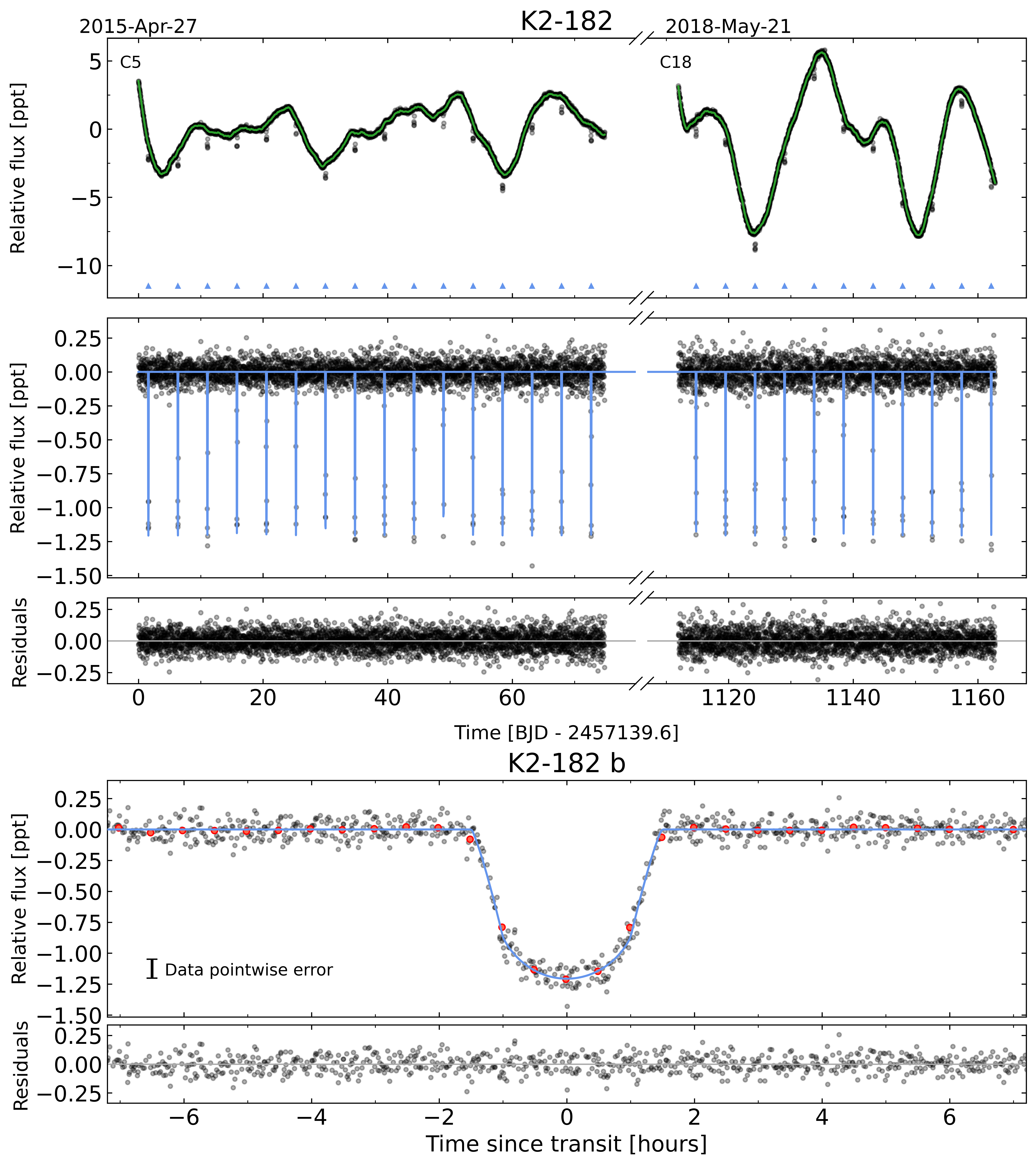
Figure 1: The maximum a posteriori (MAP) solution for the K2-182 photometric model and phase-folded transit of K2-182 b. Top: The EVEREST C5 and C18 light curves are shown as the black points. The Gaussian process ($+$ a constant offset fit to the data) used to model stellar activity is overplotted in green. Blue triangles denote K2-182 b transits. Middle: Data minus the GP model of the stellar activity are shown as the black points with the K2-182 b orbital solution from starry shown in blue. Residuals are shown below. Bottom: The phase-folded best-fitting transit model for K2-182 b and residuals. Data minus the GP model of the stellar activity are shown in black, and these data binned by 0.5 hours are shown in red. The MAP transit model is shown as the solid blue line.

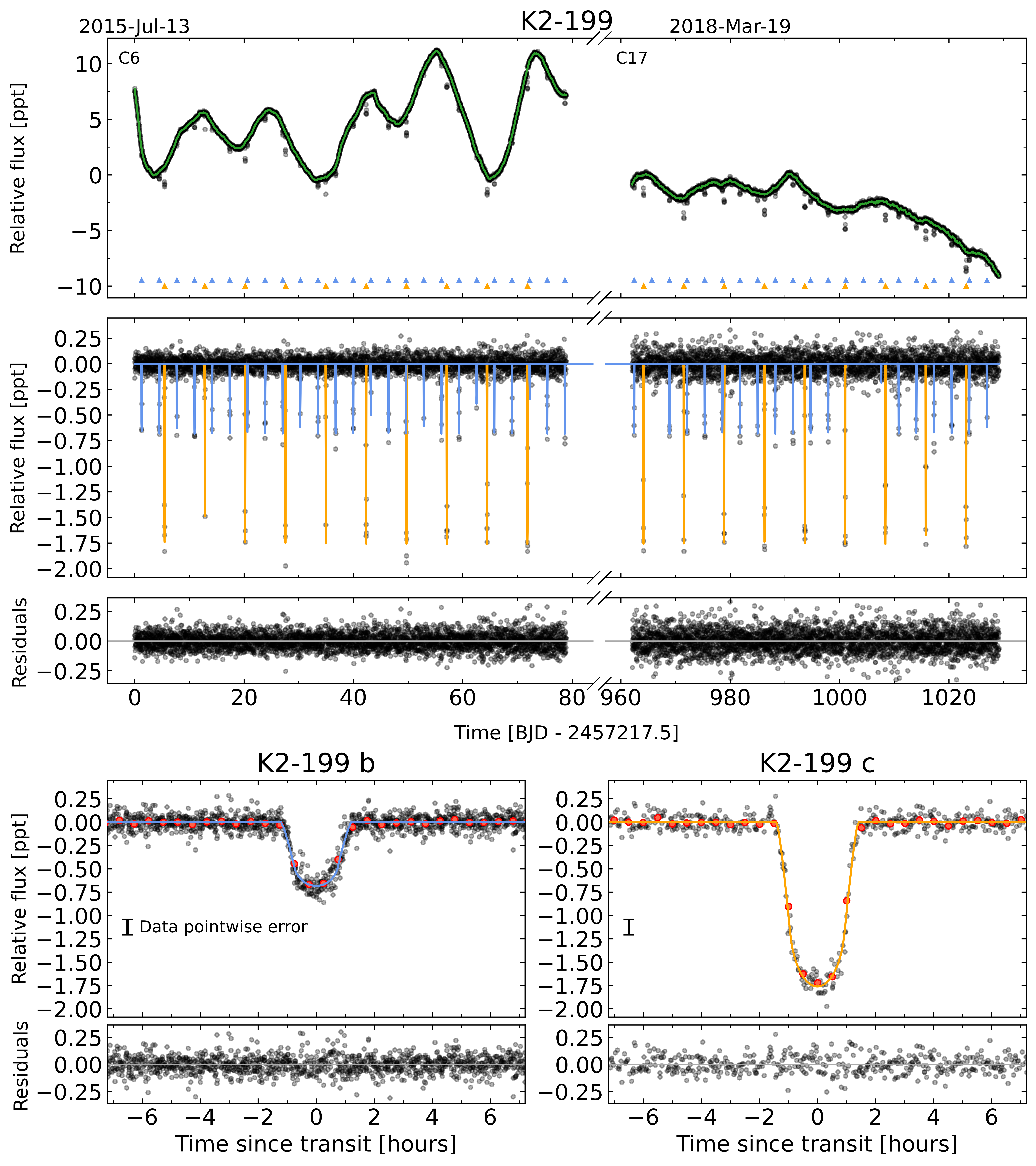
Figure 2: The MAP solution for the K2-199 photometric model and phase-folded transits of K2-199 b and c. The figure layout is analogous to Figure 1. Top: The EVEREST C6 and C17 light curves are shown as the black points. The Gaussian process ($+$ a constant offset fit to the data) used to model stellar activity is overplotted in green. Blue and orange triangles denote K2-199 b and c transits, respectively. Middle: Data minus the GP model of the stellar activity are shown as the black points with the K2-199 b and c orbital solutions from starry shown in blue and orange, respectively. Residuals are shown below. Bottom: The phase-folded best-fitting transit models for K2-199 b and c with their residuals below. Data minus the GP model of the stellar activity are shown in black, and these data binned by 0.5 hours are shown in red. The MAP transit models are shown as the solid blue and orange lines.

2.4 Posterior estimation

Implemented with exoplanet and pymc3 (Salvatier et al., 2016a), we used No-U-Turn sampling (NUTS; Hoffman & Gelman 2014), an adaptive form of Hamiltonian Monte Carlo (HMC; Duane et al. 1987 and Neal 2012), to estimate the posterior distributions of the parameters in our models of the K2 photometry. HMC sampling uses the gradient of the posterior to help inform Markov transitions, enabling more efficient exploration of high-dimensional posterior surfaces than brute-force, guess-and-check methods like Metropolis-Hastings (Metropolis et al. 1953 and Hastings 1970). For each system, a NUTS sampler ran 20 chains with starting locations randomly drawn from the model prior and with each chain taking 15,000 “tuning” steps before drawing 10,000 samples. During the tuning stage the NUTS sampler optimizes hyperparameters like step size to meet a targeted sample acceptance rate as it explores the posterior surface. This can help prevent the sampler from taking too large of a step in posterior regions with high curvature. Samples drawn during the tuning period were discarded, similar to how various Markov Chain Monte Carlo (MCMC) methods discard burn-in samples. The chains were concatenated to produce a total of $N$ = 200,000 samples from the marginal posteriors of each model parameter.

Convergence of the HMC sampling was assessed through multiple diagnostic statistics. Recently, Vehtari et al. (2019) pointed out serious flaws with the standard Gelman-Rubin statistic ($\hat{R}$; Gelman & Rubin 1992), which is conventionally used to determine convergence for iterative stochastic algorithms like MCMC. Following their prescription, we instead assessed convergence by verifying a sufficiently small ($<1.001$) rank-normalized $\hat{R}$ for each model parameter. In brief, a rank-normalized $\hat{R}$ statistic is computed by calculating $\hat{R}$ on the normalized, rank-transformed chains of the parameter, rather than the values of the parameter itself. To ensure the chains could offer reliable confidence intervals, we also calculated the rank-normalized bulk and tail effective sample sizes from Vehtari et al. (2019) for each of the marginal posteriors (roughly, the effective sample sizes are the number of “independent” samples obtained in the bulk and tails of the posterior). Vehtari et al. (2019) recommend that the effective sample size should be larger than 400 in both the bulk and the tails of the posterior. For every parameter we find the minimum between the bulk and tail effective sample sizes was much larger than the recommended minimum threshold ($N_{\mathrm{eff}}\gtrsim$ 30,000).

To avoid sampling bias, for several physical parameters (e.g. planet orbital period, planet radius, and stellar rotation period) we fit and explored the posterior of the natural logarithm of the parameter of interest. For parameters which are strictly non-negative, a prior’s hard bound at 0 can cause the posterior surface to form a “funnel” geometry, infamous of hierarchical models (Neal, 2003). NUTS sampling can have difficulty exploring the funnel because of its high curvature, which can cause the gradient calculation to diverge (Betancourt & Girolami, 2013). Fitting the natural logarithm of strictly non-negative parameters rather than the parameter itself can help to avoid the funnel geometry altogether, thereby increasing sampling efficiency and the effective sample size.

The relevant measured and derived physical planet parameters from our photometric analysis are listed in Table 1. Full lists of the parameters, priors, and posterior median values and 68% confidence intervals for our photometric models of K2-182 and K2-199 are shown in Table 2 and Table 3, respectively. In general, we used conservatively broad priors for all physical parameters save for stellar mass and radius, which had informed Gaussian priors stemming from our stellar characterization described in §3. We also used the mixture distribution from Van Eylen et al. (2019) to place a prior on planet eccentricity and marginalized over its hyperparameters.

While some of the GP hyperparameters that define the stellar activity kernel in Equation 12 are not necessarily of immediate physical interest (e.g. $f$, the mixture fraction between the SHO at $P_{\mathrm{rot}}$ and $P_{\mathrm{rot}}/2$), it can still be a useful sanity check to compare hyperparameter posteriors to physical expectations. We used Equation 11 from Kawaler (1989) to obtain a rough estimate of the expected stellar rotation period for K2-182 and K2-199 based on the (poorly-constrained) stellar ages we determined via high-resolution spectroscopy and isochrone modeling (see §3, also Table 1) and their $B-V$ colors from the EPIC catalog (Huber et al., 2016). For K2-182, the relation from Kawaler (1989) estimates $P_{\mathrm{rot}}=21\pm 2$ days. The GP model of the K2-182 stellar variability seems to agree reasonably well, finding $P_{\mathrm{rot}}=24.8\pm 1.1$ days. For K2-199, the Kawaler (1989) relation implies $P_{\mathrm{rot}}=37\pm 4$ days. However, the GP included to model the K2-199 light curves initially had difficulty inferring $P_{\mathrm{rot}}$ because the posterior was multimodal, perhaps due to the stark change in spot behavior between the two campaigns of photometry (see the top panel of Figure 2). We placed a tight prior on $P_{\mathrm{rot}}$ (really, on $\log P_{\mathrm{rot}}$) for the K2-199 GP to avoid the multimodality, so $P_{\mathrm{rot}}$ for this system should not be thought of as an inference of the stellar rotation period, but simply as a model parameter used to help flatten the light curves. We discuss this choice more in §4.2.2 and the note below Table 3.

2.5 Improvement on the precision of planet ephemerides and implications for future transit observations

K2-182 and K2-199 are particularly attractive systems for follow-up investigation because they each have two K2 campaigns of photometry. The existence of multi-campaign photometry allows us to characterize stellar variability and improve upon the orbital ephemerides. Until now the literature for these systems has lacked a joint analysis of the multi-campaign K2 observations. Furthermore, for K2-199 b Crossfield et al. (2018) note that the ephemerides they derive from the C17 data disagree with those derived from the C6 data by L18 at the 2 to 3-$\sigma$ level. With JWST primed to usher in a new era in atmospheric studies for the sub-Neptune population, precise planet ephemerides are crucial for scheduling spectroscopic transit observations. This is especially important for K2 planets compared to those from TESS, which will have been observed much more recently relative to the planned JWST launch in 2021 Nov or later.

We compared the uncertainties on our orbital period ($P$) and $T_{\mathrm{c}}$ measurements as reported in Table 1 to those in the planet validation papers, M18 and L18. For K2-199 b and c we also compared our uncertainties to Crossfield et al. (2018). For K2-182 b, our uncertainties on $P$ and $T_{\mathrm{c}}$ are improvements by a factor of about 30 and 2, respectively, over the values reported in both M18 and L18. For K2-199 b we find improvements by a factor of about 30 and 2 over the $P$ and $T_{\mathrm{c}}$ values in M18 and improvement factors of $\gtrsim 60$ and $3$ compared to both L18 and Crossfield et al. (2018). We find similar improvement factors in each case for K2-199 c. Figure 3 visualizes how our refinement of $P$ and $T_{\mathrm{c}}$ greatly reduce the transit time uncertainty for each planet over the next decade compared to the literature values. Our improvements to the ephemerides are key in making these planets viable targets for future space-based missions like JWST.

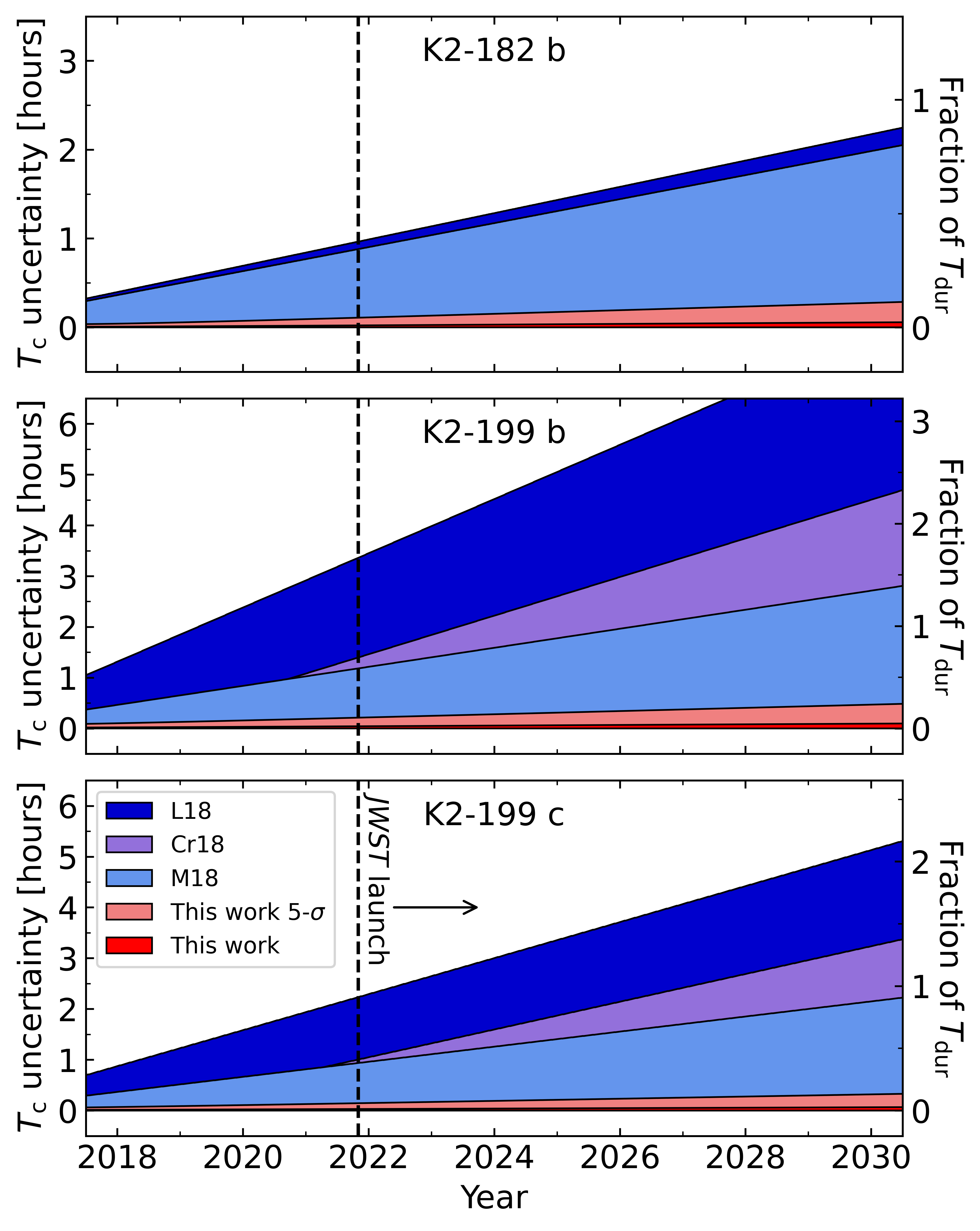
Figure 3: Transit time uncertainty for the three planets over the next decade. The left and right axes show the uncertainty in units of hours and as a fraction of the transit duration, respectively. Regions for L18, Cr18, and M18 refer to the 1-$\sigma$ uncertainty in $T_{\mathrm{c}}$ as propagated from the values in Livingston et al. (2018), Crossfield et al. (2018), and Mayo et al. (2018), respectively. Note that Crossfield et al. (2018) analyzed K2 C17 and therefore does not include K2-182 b. 1-$\sigma$ and 5-$\sigma$ uncertainties in $T_{\mathrm{c}}$ over time are also plotted using the refined ephemerides from this work. The dashed vertical line and arrow mark JWST’s launch in 2021 Nov or later. With our measurements of $P$ and $T_{\mathrm{c}}$, the 5-$\sigma$ uncertainty in the transit time of each planet will be less than 20 minutes by the year 2025.

3 Stellar characterization

3.1 High-resolution spectroscopy

We used the High Resolution Echelle Spectrometer (HIRES; Vogt et al. 1994) on the 10-m Keck I telescope at the W. M. Keck Observatory on Mauna Kea to obtain an iodine-free (see §4.1) spectrum of K2-182 at high resolution and high signal-to-noise (a “template” spectrum). For K2-199 we used the Keck-HIRES template from Howard et al. (in prep). These spectra were collected with the B3 decker (14″$\times$0″.574, $R=67,000$), the length of which allows for effective sky-subtraction (important for these $V>12$ mag stars). The templates were obtained on UTC 2019 May 7 and 2017 Feb 3 for K2-182 and K2-199, respectively, with exposure times of 2700 s. K2-182 was observed at an airmass of 1.33 and K2-199 was observed at an airmass of 1.14. The K2-182 and K2-199 templates have a signal-to-noise ratio (SNR) of 173/pix and 163/pix, respectively, as measured at 5500 Å. Both templates were collected while the moon was below the horizon. Triple-shot exposures of rapidly-rotating B stars were taken with the iodine cell in the light path immediately before and after the high-resolution spectra were collected to precisely constrain the instrumental point spread function (PSF). The data collection and reduction followed the methods of the California Planet Search as described in Howard et al. (2010).

We used SpecMatch-Syn (Petigura 2015 and applied by Petigura et al. 2017b) to constrain the stellar effective temperature ($T_{\mathrm{eff}}$), surface gravity ($\log g$), and metallicity ([Fe/H]) of K2-182 directly from our high-SNR, iodine-free Keck-HIRES template. SpecMatch-Syn fits segments of optical spectra (380 Å between 5200 and 6260 Å) by interpolating on a three-dimensional grid (in $T_{\mathrm{eff}}$, $\log g$, and [Fe/H]) of synthetic spectral models (Coelho et al., 2005). The interpolated spectrum is then convovled with the kernel from Hirano et al. (2011) to account for rotational line broadening, as well as with a Gaussian that represents the Keck-HIRES PSF during typical seeing conditions. For K2-182, SpecMatch-Syn finds $T_{\text{eff}}=5170\pm 100$ K, $\log g$ $=4.61\pm 0.10$ dex, and $\text{[Fe/H]}=0.12\pm 0.06$ dex.

K2-199 is a K5V-dwarf (Dressing et al., 2017). We used SpecMatch-Emp (Yee et al., 2017) to constrain K2-199’s $T_{\mathrm{eff}}$, stellar radius ($R_{*}$), and [Fe/H] from the template spectra collected by Howard et al. (in prep). SpecMatch-Emp fits stellar spectra between 5000 and 5800 Å in 100 Å segments using linear combinations of spectral templates from a library of over 400 precisely-characterized FGKM stars. For our initial characterization of K2-199 we chose to use SpecMatch-Emp rather SpecMatch-Syn because the former is robust to cooler stars ($\sim$K4 and later) whose molecular spectral features may not be accounted for in synthetic models. For K2-199, SpecMatch-Emp finds $T_{\mathrm{eff}}=4491\pm 70$ K, [Fe/H] $=-0.01\pm 0.09$ dex, and $R_{*}=0.70\pm 0.10$ $R_{\odot}$.

To derive the final stellar parameters, we compiled the results from SpecMatch-Syn and SpecMatch-Emp with parallaxes from the second Gaia data release (Gaia DR2; Gaia Collaboration et al. 2016, 2018; Luri et al. 2018) and multiband photometry (Gaia $G$ and Two Micron All Sky Survey [2MASS] $JHK$, Cutri et al. 2003). We then input these data to isoclassify (Huber et al. 2017 and Berger et al. 2020), using grid mode. isoclassify infers marginal posteriors for stellar parameters by integrating over a grid of MIST isochrones (Choi et al., 2016). The stellar parameters are summarized in Table 1. We find that our derived stellar parameters are generally consistent to within 1 to 2-$\sigma$ of those reported in the validation papers. We note that M18 was published in March 2018, before Gaia DR2 became public. L18 was published in November 2018 and incorporated Gaia DR2 parallaxes in the determination of stellar properties.

While our methodology for the stellar characterization closely follows the procedure in L18—who use iodine-free Keck-HIRES spectra ($\text{SNR}\approx 40\text{/pixel}$) obtained by Petigura et al. (2017a)—we chose to re-derive the stellar parameters ourselves because the templates we feed to SpecMatch-Syn and SpecMatch-Emp have much higher SNR. Additionally, we note that in their derivation of stellar parameters, L18 use SpecMatch-Syn for K2-199 rather than SpecMatch-Emp. This is in contrast to Petigura et al. (2017a), who used the latter—L18 only use SpecMatch-Emp for stars cooler than 4200 K, while Petigura et al. (2017a) use it for stars cooler than 4600 K. For completeness, we tried using the K2-199 SpecMatch-Syn outputs as inputs to isoclassify (along with the Gaia DR2 parallax and multiband photometry) and found all stellar parameters to be 1-$\sigma$ consistent with the values in Table 1. Moving forward we choose to quote the isoclassify results that take input from SpecMatch-Syn for K2-182 and SpecMatch-Emp for K2-199 because this follows the $T_{\mathrm{eff}}$ threshold from Petigura et al. (2017a).

While we do not report a precise spectral classification for K2-182, we suggest it is an early-K dwarf based on SpecMatch-Emp, which models its spectrum as a linear combination of GL 144, HD 8553, HD 80367, HD 170657, and HD 189733, all of which are K0V to K2V.

Table 1: System parameters

Identifying information
EPIC ID			211359660	212779596	EPIC
Right ascension	RA	deg (J2000)	$130.18004$	$208.90145$	Gaia DR2
Declination	DEC	deg (J2000)	$10.98295$	$-6.13608$	Gaia DR2
Kepler magnitude	$K_{\mathrm{p}}$	mag	11.74	11.93	EPIC
Spectroscopy
Effective temperature	$T_{\mathrm{eff}}$	K	$5170\pm 100$	$4491\pm 100$	SpecMatcha
Surface gravity	$\log g$	cgs	$4.61\pm 0.10$	$\cdots$	SpecMatcha
Metallicity	[Fe/H]	dex	$0.12\pm 0.06$	$-0.01\pm 0.09$	SpecMatcha
Isochrone modeling
Mass	$M_{*}$	$M_{\odot}$	$0.865^{+0.016}_{-0.018}$	$0.711^{+0.022}_{-0.024}$	isoclassify
Radius	$R_{*}$	$R_{\odot}$	$0.793^{+0.013}_{-0.011}$	$0.682\pm 0.014$	isoclassify
Luminosity	$L$	$L_{\odot}$	$0.391^{+0.014}_{-0.012}$	$0.185\pm 0.010$	isoclassify
Age		Gyr	$2.07^{+2.14}_{-1.36}$	$5.04^{+6.12}_{-3.59}$	isoclassify
Planet Parameters
Parameter	Symbol	Units	K2-182 b	K2-199 b	K2-199 c
Measured quantities
Orbital period	$P$	Days	$4.7369683\pm 0.0000023$	$3.2253993\pm 0.0000024$	$7.3744897\pm 0.0000037$
Time of inferior conjunction	$T_{\mathrm{c}}$	$\mathrm{BJD}-2454833$	$2886.11517\pm 0.00028$	$2385.73733^{+0.00051}_{-0.00055}$	$2389.93034\pm 0.00035$
Occultation fraction	$\frac{R_{\mathrm{p}}}{R_{*}}$	%	$3.111^{+0.063}_{-0.052}$	$2.346^{+0.043}_{-0.038}$	$3.846^{+0.089}_{-0.077}$
Impact parameter	$b$		$0.20^{+0.19}_{-0.13}$	$0.25^{+0.12}_{-0.15}$	$0.49^{+0.06}_{-0.08}$
Orbital eccentricityb	$e$		$0.04^{+0.19}_{-0.03}$	$0.02^{+0.03}_{-0.02}$	$0.03^{+0.06}_{-0.03}$
Argument of periastronb	$\omega$	rad	$3.7^{+2.0}_{-2.2}$	$3.0^{+2.3}_{-2.1}$	$2.9^{+2.3}_{-2.0}$
RV semi-amplitude	$K$	m s-1	$8.4\pm 2.0$	$3.8\pm 1.0$	$5.1\pm 1.0$
Derived quantities
Transit duration	$T_{\mathrm{dur}}$	Hours	$2.561^{+0.056}_{-0.143}$	$2.017^{+0.049}_{-0.054}$	$2.452^{+0.097}_{-0.081}$
Orbital inclination	$i$	Rad	$1.56\pm 0.01$	$1.55\pm 0.01$	$1.53\pm 0.01$
Orbital separation	$\frac{a}{R_{*}}$		$14.23\pm 0.22$	$12.07^{+0.26}_{-0.27}$	$20.96^{+0.46}_{-0.48}$
Orbital semi-major axis	$a$	AU	$0.0526\pm 0.0003$	$0.0382\pm 0.0004$	$0.0662\pm 0.0007$
Radius	$R_{\mathrm{p}}$	$R_{\oplus}$	$2.69^{+0.07}_{-0.05}$	$1.73^{+0.05}_{-0.04}$	$2.85^{+0.10}_{-0.09}$
Mass	$M_{\mathrm{p}}$	$M_{\oplus}$	$20\pm 5$	$6.9\pm 1.8$	$12.4\pm 2.3$
Bulk density	$\rho$	g cm-3	$5.6\pm 1.4$	$7.2^{+2.1}_{-2.0}$	$2.9^{+0.7}_{-0.6}$
Equilibrium temperaturec	$T_{\mathrm{eq}}$	K	$969\pm 20$	$913\pm 23$	$694\pm 17$
Instellation flux	$S_{\mathrm{p}}$	$S_{\oplus}$	$146.9^{+12.6}_{-11.8}$	$116.2^{+12.0}_{-11.0}$	$38.6\pm 4.0$
Core water mass fractiond	$f_{H_{2}O}$	%	$45^{+26}_{-20}$	$14^{+25}_{-11}$	$88^{+8}_{-14}$
H2/He envelope mass fractione	$f_{\mathrm{env}}$	%	$\cdots$	$0.03^{+0.04}_{-0.01}$	$2.9\pm 0.6$
TSMf	TSM		$16^{+5}_{-3}$	$17^{+6}_{-4}$	$32^{+9}_{-6}$

Note. — Values reported in this table represent medians of the marginal posterior, while errors reflect the the upper and lower bounds of the 68% confidence interval about the median. Errors on derived planetary parameters include errors on stellar mass and radius by way of Gaussian priors placed on the stellar properties (informed by our stellar characterization) during the modeling of the photometry and radial velocities.
a: SpecMatch-Syn was used for K2-182 and SpecMatch-Emp was used for K2-199 following the $T_{\mathrm{eff}}$ threshold of Petigura et al. (2017a).

b: $e$ and $\omega$ were allowed to vary during the light curve modeling. Finding that the orbits were consistent with circular, they were held fixed at zero in models of the RVs.
c: Equilibrium temperature calculated assuming zero Bond albedo.

d: Core water mass fraction calculated assuming a bulk composition of water and rock, using the grid from Zeng et al. (2016).

e: H₂/He envelope mass fraction calculated assuming a $1\times$ solar metallicity H₂/He envelope on top of an Earth-like rock/iron core, using the grids from Lopez & Fortney (2014). We do not infer $f_{\mathrm{env}}$ for K2-182 b because its mass lies at the edge of the grid (20 $M_{\oplus}$).

f: The transmission spectroscopy metric from Kempton et al. (2018).

References for the provenance values in the order in which they appear in the table: EPIC (Ecliptic Plane Input Catalog; Huber et al. 2016), Gaia DR2 (Gaia Collaboration et al. 2016, 2018), isoclassify (Huber et al. 2017 and Berger et al. 2020).

3.2 High-resolution imaging

High-resolution imaging is a key component of the planet validation process because it can rule out astrophysical false positive scenarios and put limits on dilution levels from nearby stellar contaminants. While all three planets were previously validated by M18 and L18, we acquired new (in the case of K2-182) and reduced publicly available (for K2-199) high-resolution, high-contrast imaging observations in an attempt to further improve contrast limits.

3.2.1 K2-182

Neither M18 or L18 included imaging in their vespa FPP calculations for K2-182 b. While Gaia DR2 does not detect any bright sources within the EVEREST aperture, we observed K2-182 with the second-generation Near-infrared Camera (NIRC2; Wizinowich et al. 2014) on the Keck II telescope to confidently rule out nearby stellar contaminants.

K2-182 was observed with Keck-NIRC2 on UT 2020 May 28 at an airmass of 1.58. Observations were taken in narrow camera mode with a 1024” x 1024” FOV. A three-point dither pattern was used to avoid the noisy fourth quadrant of the detector. Observations were taken in the $K$ filter for a total integration time of 4 seconds.

All of the Keck-NIRC2 AO data were processed and analyzed with a custom set of IDL tools. The science frames were flat-fielded and sky-subtracted. The flat fields were generated from a median average of dark subtracted flats taken on-sky. The flats were normalized such that the median value of the flats is unity. The sky frames were generated for each observation set individually; the dithered flat-fielded science frames were median averaged to produce a single sky frame that was then subtracted from all of the flat-field science frames. The reduced science frames were combined into a single combined image using a intra-pixel interpolation that conserves flux, shifts the individual dithered frames by the appropriate fractional pixels, and coadds the frames. The final resolution of the combined dither was determined from the full-width half-maximum of the point spread function.

The sensitivities of the final combined Keck-NIRC2 image were determined by injecting simulated sources azimuthally around the primary target every $45\degree$ at separations of integer multiples of the central source’s full width at half maximum (FWHM; Furlan et al. 2017). The brightness of each injected source was scaled until standard aperture photometry detected it with 5-$\sigma$ significance. The resulting brightness of the injected sources relative to the target set the contrast limits at that injection location. The final 5-$\sigma$ limit at each separation was determined from the average of all of the determined limits at that separation and the uncertainty on the limit was set by the RMS dispersion of the azimuthal slices at a given radial distance.

From our Keck-NIRC2 imaging of K2-182 we find no companions to 5-$\sigma$ confidence for $\Delta K=5.1$ mag at a minimum separation of 0″.2 and for $\Delta K=7.0$ mag at a minimum separation of 0″.5. We find no companions to 5-$\sigma$ confidence for $\Delta K=7.4$ mag at a minimum separation of 1″. The Keck-NIRC2 image is shown on the left in Figure 4.

All of our observations suggest that K2-182 is unambiguously single. If there was an undetected source within $\sim$1″, we would expect to see it in our spectroscopic observations. However, using the methodology from Kolbl et al. (2015), we find no indication that K2-182 is a double-lined spectroscopic binary (and the Kolbl et al. 2015 algorithm is sensitive to companions down to $\sim$1% the brightness of the primary in $V$-band). Furthermore, if there did happen to be an undetected source that our imaging is unable to rule out, even in the “worst case scenario” (i.e. a $\Delta K=7.4$ mag neighbor at a separation of 1″) the dilution level would be negligible at $<1\%$.

3.2.2 K2-199

As explained in §2.1, although a fainter neighbor falls in our EVEREST aperture for K2-199 ($\Delta K_{\mathrm{p}}=5.6$ mag, separation $\approx 8$″) any contamination from this source would be $<1\%$ and is therefore negligible compared to our other sources of error (e.g. stellar properties).

L18 and M18 use observations of K2-199 from the Differential Speckle Survey Instrument (DSSI; Horch et al. 2009) on both the WIYN telescope at KPNO and the 8.1-m Gemini-North telescope at the Gemini North Observatory on Mauna Kea to inform their vespa FPP calculations. Two images, one centered at 6920 Å and one centered at 8800 Å, were taken with both WIYN and Gemini-North. The WIYN images were taken on UT 2016 Apr 21 and have an estimated contrast of $\Delta$3.5 mag at a separation of 0″.2. The Gemini-North images were taken on UT 2016 Jun 21 and have an estimated contrast of $\Delta$5.0 mag at a separation of 0″.2.

To improve contrast limits beyond those from DSSI, we identified and reduced a publicly available, archival AO image of K2-199 from Keck-NIRC2. The archival Keck-NIRC2 image was acquired on UT 2016 Apr 21 at an airmass of 1.12. The observations were taken in the $K_{\mathrm{s}}$ filter with a total integration time of 288 seconds. Our data reduction for the archival image mimicked our method for the Keck-NIRC2 image of K2-182. We find no companions at 5-$\sigma$ confidence for $\Delta K_{\mathrm{s}}=4.4$ mag at 0″.2 separation, $\Delta K_{\mathrm{s}}=6.9$ mag at 0.″5 separation, and $\Delta K_{\mathrm{s}}=8.8$ mag at 1″ separation. The high-resolution image from Keck-NIRC2 is shown on the right in Figure 4.

Similar to the case for K2-182, our observations of K2-199 suggest that the star is unambiguously single. We find no evidence that K2-199 is a double-lined spectroscopic binary (Kolbl et al., 2015). Any dilution from a neighbor that was not detected by the imaging observations would be $<1\%$, making its impact on the derived planetary radii negligible.

Figure 4: Our high-resolution, high-contrast images of K2-182 and K2-199. Left: The high-resolution image of K2-182 with Keck-NIRC2. The Keck-NIRC2 image rules out companions at 5-$\sigma$ confidence with a maximum contrast of $\Delta K=7.4$ mag at a minimum separation of 1″. Right: The Keck-NIRC2 image of K2-199 that we reduced from archival observations. We rule out nearby companions at 5-$\sigma$ confidence down to $\Delta K_{\mathrm{s}}=8.8$ mag at a minimum separation of 1″.

4 Radial velocities

4.1 Observations

We obtained 12 high-resolution spectra of both K2-182 and K2-199 with Keck-HIRES to measure precise radial velocities (RVs). The observations of K2-182 were taken between UTC 2019 Mar 27 and 2019 May 29 with a median exposure time of 1208 seconds and a median SNR of 100/pixel. The observations of K2-199 were taken between UTC 2019 Feb 18 and 2019 May 30 with a median exposure time of 1402 seconds and a median SNR of 100/pixel. All spectra were collected with the C2 decker (14″$\times$0″.86, $R=$ 60,000) to allow for sky subtraction.

Radial velocities were determined following the procedures of Howard et al. (2010). In brief, a warm ($50\degree$ C) cell of molecular iodine was placed at the entrance slit during the RV observations (Butler et al., 1996). The superposition of the iodine absorption lines on the stellar spectrum provides both a fiducial wavelength solution and a precise, observation-specific characterization of the instrument’s PSF. Each RV spectrum was then modeled as the sum of the deconvolved template spectrum (see §3.1) and the instrumental PSF convolved with an “infinite resolution” laboratory spectrum of the molecular iodine. Our RV measurements of K2-182 and K2-199 are listed in Table 6 and Table 7, respectively. Before applying any models, the K2-182 RV data had an RMS of 6.88 m s^-1 and a median pointwise error of 1.55 m s^-1. The K2-199 RVs had an RMS of 5.21 m s^-1 and a median pointwise error of 1.73 m s^-1.

For our analysis of K2-199 we include 33 Keck-HIRES iodine-in spectra from Howard et al. (in prep), which were obtained between UTC 2016 Jul 23 and 2018 Mar 17. These observations were also collected with the C2 decker and RVs of the combined ($N=45$) data set were derived simultaneously. Before applying any models, the combined K2-199 RV data had an RMS of 6.31 m s^-1 and a median pointwise error of 1.69 m s^-1.

4.2 Stellar activity

Failure to account for just one coherent signal in an RV time series (e.g. stellar activity, additional planets, instrumental systematics) can produce discrepant planet mass measurements, even in the presence of large data sets (Rajpaul et al., 2017). As RV observations enter the era of sub-m s^-1 measurement precision with next-generation instruments like Gemini-MAROON-X (Seifahrt et al., 2016) and WIYN-NEID (Schwab et al., 2016), confounding signals in RV data, astrophysical or otherwise, will become the limiting factor in the pursuit of precise mass measurements for small planets.

Stellar activity can produce RV signals across a range of timescales by distorting spectral line profiles. As summarized by Vanderburg et al. (2016), asteroseismic oscillations, granulation, starspots, and stellar magnetic activity can produce RV amplitudes on the order of 1 to several m s^-1 for timescales of a few minutes, to hours and days, to months, and even years for stellar magnetic cycles (Butler et al. 2004, Dumusque et al. 2011, Queloz et al. 2001, Gomes da Silva et al. 2012). When the dominant stellar activity timescale is sufficiently short (typically minutes to a few days), it is common to treat the RV-signature of the activity as additional white noise about the planetary signal(s), added in quadrature with the pointwise RV measurement errors (Gregory, 2005). However, adding a simple “RV jitter” term to the likelihood function can prove insufficient when correlated stellar activity signals extend to longer timescales ($\sim$tens of days). Vanderburg et al. (2016) show that the RV signals of rotating starspots can confuse planet searches, especially when the stellar rotation period and its first two harmonics fall near planet orbital periods.

As seen from their K2 light curves, both K2-182 and K2-199 exhibit clear signs of starspots and spot modulation as well as significant spot evolution from one campaign to another. To obtain a rough estimate of the amplitude of the systematic RV contributions due to star spots ($\sigma_{\mathrm{RV,\>spot}}$), following Dragomir et al. (2019) we adapted Equation 2 from Vanderburg et al. (2016) as $\sigma_{\mathrm{RV,\>spot}}\approx\sigma_{\mathrm{phot}}\times v\sin i$, where $\sigma_{\mathrm{phot}}$ is the standard deviation of the light curve flux and $v\sin i$ is the sky-project stellar rotational velocity.

For K2-182, $\sigma_{\mathrm{phot}}=0.0026$ in units of relative flux from the EVEREST C5 and C18 light curves and SpecMatch-Syn finds $v\sin i=0.25\pm 1.0$ km s^-1 from our Keck-HIRES template spectra. However, SpecMatch-Syn $v\sin i$ estimates below 2.0 km s^-1 should be interpreted as less than 2 km s^-1. Using $2$ km s^-1 as an upper limit on $v\sin i$ we calculate $\sigma_{\mathrm{RV,\>spot}}\lesssim 5.2$ m s^-1. Since SpecMatch-Syn only provides an upper limit on $v\sin i$ for K2-182, we also calculated $\sigma_{\mathrm{RV,\>spot}}$ using $v\sin i=2\pi R_{*}\sin i/P_{\mathrm{rot}}$ and $\sin i\approx 1$, where $R_{*}=0.79$ $R_{\odot}$ (Table 1) and $P_{\mathrm{rot}}\approx 25$ days (see 4.2.1). Estimating $v$ with $R_{*}$ and $P_{\mathrm{rot}}$, we find $\sigma_{\mathrm{RV,\>spot}}\approx 4.2$ m s^-1.

For K2-199, the EVEREST C6 and C17 light curves have $\sigma_{\mathrm{phot}}=0.0027$. While SpecMatch-Emp does not calculate an absolute $v\sin i$, SpecMatch-Syn finds $v\sin i<2$ km s^-1 from the Keck-HIRES template. Given our discussion in §3.1, though, K2-199 is too cool for SpecMatch-Syn. Modulo this concern, $\sigma_{\mathrm{RV,\>spot}}$ would be $\lesssim 5.4$ m s^-1 for K2-199 using the SpecMatch-Syn upper limit. Extracting $P_{\mathrm{rot}}$ from the K2 photometry was nontrivial for K2-199 (see 4.2.2), so we do not try to estimate $\sigma_{\mathrm{RV,\>spot}}$ via $R_{*}$ and $P_{\mathrm{rot}}$ for K2-199 as we did for K2-182.

We employed a GP to model the RV-signatures of stellar activity in an attempt to mitigate their impact on the planet mass measurements. GPs are a popular tool for modeling correlated stellar activity and can help inform RV models when trained on complementary data such as photometry (Haywood et al., 2014; Grunblatt et al., 2015) or activity indicators like Ca II H and K emission ($S_{\text{HK}}$; Isaacson & Fischer 2010; Kosiarek et al. 2021) and H-$\alpha$ indices (Robertson et al., 2013). Recently, Kosiarek & Crossfield (2020) used over 70 years of solar observations to demonstrate that photometry can act as a proxy for stellar activity in GP-enabled analyses. Below we discuss the results of training GPs on the K2-182 and K2-199 photometry.

4.2.1 K2-182

K2-182 is an early-K dwarf. Ca II H and K emission indicates it is moderately active—using the iodine-free Keck-HIRES template we find $\log R^{\prime}_{\text{HK}}=-4.68$ dex (Middelkoop, 1982; Noyes et al., 1984). For reference, over its magnetic cycle the Sun floats between $\log R^{\prime}_{\text{HK}}=-5.05$ and $-4.84$ dex (Meunier et al., 2010). We used a GP with a quasi-periodic (QP) kernel to model the stellar rotation and spot modulation seen in the K2 C5 and C18 photometry. The kernel,

$$k(t,t^{\prime})=\eta_{1}^{2}\ \mathrm{exp}\left[-\frac{(t-t^{\prime})^{2}}{\eta_{2}^{2}}-\frac{\sin^{2}(\frac{\pi(t-t^{\prime})}{\eta_{3}})}{2\eta_{4}^{2}}\right],$$ (13)

quantifies the covariance between data observed at times $t$ and $t^{\prime}$. $\eta_{\text{1-4}}$ are the hyperparameters: $\eta_{1}$ represents the amplitude of the covariance, $\eta_{2}$ is interpreted as the evolutionary timescale of active stellar regions, $\eta_{3}$ is interpreted as the stellar rotation period, and $\eta_{4}$ is the length scale of the covariance’s periodicity. The GP “training” consists of performing a MAP fit to the training data (the out-of-transit K2 photometry) and posterior estimation for the GP hyperparameters with MCMC. The posteriors of $\eta_{2}$, $\eta_{3}$, and $\eta_{4}$ resulting from the training step are then used as numerical priors for these hyperparameters in a Keplerian $+$ GP fit to the RVs.

Although the QP kernel in Equation 13 is not the same kernel we use to simultaneously model stellar activity and planetary transits (see §2.3), the QP kernel has been shown to be an effective model of stellar light curves (e.g. Angus et al. 2018) and both kernels have the capacity to explain exponentially decaying and periodic signals. We employ the QP kernel for the GP $+$ Keplerian modeling of the RVs because it is a familiar choice for stellar activity mitigation in RV time series (e.g. Grunblatt et al., 2015; Kosiarek et al., 2021). In addition, it uses fewer free hyperparameters than the sum of SHOs we used in §2.3 (four versus seven), which is important for our smaller RV data sets. Given a covariance kernel that produces a smooth process (e.g. both the QP kernel and the sum of SHOs), even if hyperparameters differ, the GP’s posterior predictions should be similar.

The GP training on the out-of-transit K2 C5 and C18 photometry resulted in tight constraints on K2-182’s active region evolutionary timescale, stellar rotation period, and periodic length scale ($\eta_{2}=37.4\pm 5.2$ days, $\eta_{3}=24.92^{+0.26}_{-0.21}$ days, and $\eta_{4}=0.350^{+0.019}_{-0.018}$, respectively). This estimate of the stellar rotation period is consistent with the rotation period derived by the GP used to model the stellar activity signal in the K2-182 photometry in §2.3 ($P_{\mathrm{rot}}=$ $24.80\pm 1.1$ days). The posteriors on $\eta_{2}$, $\eta_{3}$, and $\eta_{4}$ were used as priors for an RV model that included a GP component, as described in §4.3.1.

While Keck-HIRES $S_{\text{HK}}$ values were measured simultaneously with RV observations, we forgo using them to inform models of correlated stellar activity given the small size of the data set. Our K2-182 data set is also too small for a meaningful periodogram analysis so we reserve a discussion of the RV, RV residuals, and $S_{\text{HK}}$ periodograms for K2-199.

4.2.2 K2-199

K2-199 is slightly cooler than K2-182 and has a spectral classification of K5V (Dressing et al., 2017). Ca II H and K emission indicates that it is also moderately active, with $\log R^{\prime}_{\text{HK}}=-4.65$ dex. The K2 photometry shows stark differences in spot behavior from C6 to C17 (top panel of Figure 2). While the C6 photometry appears to show a quasi-periodic signal, the amplitude of the modulation is damped significantly in C17. Using the kernel in Equation 13, training a GP on the out-of-transit C6 and C17 photometry resulted in a bimodal posterior on $\eta_{3}$, with one peak near 14.15 days and another at 17.8 days. Examining a Lomb-Scargle periodogram (Lomb, 1976; Scargle, 1982) of the K2 photometry, we find that the signal at 14.15 days is the first harmonic of a larger peak at 28.3 days. With the slight offset between the first harmonic of the peak at 28.3 days and the peak at 17.8 days, the GP had trouble modeling both signals with only a single hyperparameter to explain the periodicity ($\eta_{3}$). The kernel used to model the stellar activity signal in the photometry in §2.3, which included a periodic term at $P_{\mathrm{rot}}$ and $P_{\mathrm{rot}}/2$, also had difficulty with the bimodality (see the note for Table 3). In the end, training a GP on the K2-199 photometry could be a moot point because of the star’s apparent change in spot behavior over time—it is unclear which paradigm applies to the time period over which our RVs were collected.

In addition to experimenting with training a GP on the K2-199 photometry to search for signs of correlated stellar activity, we also examined a Lomb-Scargle periodogram of the RV times series, the RV residuals about our MAP solution from §4.3.2 (seen in Figure 6), and the $S_{\text{HK}}$ indices we measured simultaneously with the RVs. In a periodogram of the RVs, the only peak to rise above the $1\%$ false alarm probability (FAP) level is the signal of K2-199 c at $P=7.37$ days. A periodogram of the RV time series with both planets removed shows no peaks above the 10% FAP level. A periodogram of the $S_{\text{HK}}$ values reveals a peak at 359.8 days that rises above the 0.01% FAP level. However, nothing significant (above the 1% FAP level) is detected shortward of the the 359.8-day peak’s first harmonic at 179.9 days, so while there is power at these longer periods we do not believe it should affect the planetary signals ($P=3.23$ and $7.37$ days).

We choose not to pursue an RV model of K2-199 that includes a GP due to the change in K2-199’s spot behavior between campaigns and the lack of Lomb-Scargle power in the Keck-HIRES $S_{\text{HK}}$ indices on timescales comparable to the planet orbital periods. Moving forward we suggest that additional photometric monitoring, contemporaneous with RV and $S_{\text{HK}}$ observations, may help better inform the correlated RV signatures of stellar activity (if any) for K2-199 (Grunblatt et al., 2015). On the other hand, experimentation with a wider variety of GP kernels may help model the existing K2 photometry.

4.3 Radial velocity analysis

We used radvel (Fulton et al., 2018) to model the RVs. radvel uses MAP estimation to fit Keplerian orbits to an RV time series. The orbit of each planet is described using five parameters: orbital period ($P$), time of inferior conjunction ($T_{\mathrm{c}}$), orbital eccentricity ($e$), argument of periastron passage ($\omega$), and RV semi-amplitude ($K$). Modeling the velocities as a sum of Keplerian orbits and noise produces a measurement of $M_{\mathrm{p}}$ $\sin i$ for each planet, where $i$ is the planet’s orbital inclination. Using Equation 7 in Winn (2010), we derive $i$ for each planet from our models of the photometry (see Table 1), enabling the conversion from $M_{\mathrm{p}}$ $\sin i$ to $M_{\mathrm{p}}$.

radvel estimates posterior distributions with an MCMC scheme that uses an Affine Invariant sampler (Goodman & Weare, 2010) from emcee (Foreman-Mackey et al., 2013). For the MCMC uncertainty estimation we followed the default prescription for burn-in criteria, the number of walkers, the number of steps, and convergence testing as described by Fulton et al. (2018). In our analysis of the radial velocities we opted to use emcee for the posterior estimation rather than employ an HMC sampler as we did for the models of the photometry (see §2.4). The biggest benefit of using HMC over other sampling methods is to enable the efficient exploration of high-dimensional posteriors. Since our models of the radial velocities have many fewer free parameters than the models of the photometry—K2-199’s photometric model has 25 free parameters (Table 3) while our adopted model of the system’s radial velocities has seven (Table 5)—we found that posterior estimation with emcee for the models of the radial velocities was computationally tractable. Since emcee is already integrated with radvel (and pymc3, which enabled the HMC sampling for our models of the K2 photometry, is not), we chose to use emcee for posterior estimation in our radial velocity analysis.

We used the AICc, the small sample-corrected version of the Akaike Information Criterion (AIC; Akaike 1974) to compare models of the radial velocities:

$$\mathrm{AICc}=\mathrm{AIC}+\frac{2k^{2}+2k}{n-k-1},$$ (14)

where

$$\mathrm{AIC}=2k-2\log\mathcal{\hat{L}},$$ (15)

$k$ is the number of free parameters in the model, $n$ is the sample size, $\log$ is the natural logarithm, and $\mathcal{\hat{L}}$ is the maximum of the likelihood function with respect to the model parameters. The AICc is essentially the same as the AIC, but with an additional penalty term for model complexity, since the AIC has a tendency to favor models that overfit when $n$ is small. Burnham & Anderson (2002) recommend using the AICc in place of the AIC when $n\lesssim 40\times k$. Note that as $n\rightarrow+\infty$ the AICc reduces to the AIC. We elect to use the AICc over other popular model comparison metrics, namely the Bayesian Information Criterion (BIC; Schwarz 1978), because simulation studies suggest that for finite $n$, the BIC may be at risk of selecting very poor models (Burnham & Anderson, 2004; Vrieze, 2012).

Let $\Delta\mathrm{AICc}_{i}\equiv\mathrm{AICc}_{i}-\mathrm{AICc}_{\mathrm{min}}$, where AICc_i is the AICc of the $i$th model under consideration and AICc_min is the lowest AICc of all models considered. When comparing models with the AICc, Burnham & Anderson (2004) provide the following guidelines:

• If $\Delta\mathrm{AICc}_{i}<2$, the two models are nearly indistinguishable.

• If $2<\Delta\mathrm{AICc}_{i}<10$, the $i$th model is disfavored.

• If $\Delta\mathrm{AICc}_{i}>10$, the $i$th model is essentially ruled out.

4.3.1 K2-182

Our models of the K2-182 RVs hold a few common assumptions: Each model assumes there is a single planet orbiting K2-182. Additional planets would have to have an orbital period $>80$ days (the length of a normal K2 campaign) and/or be non-transiting. Our RV data set is not large enough ($N=12$) to comment on the system’s multiplicity in the absence of constraints from the K2 photometry. Each of our K2-182 models also assume a circular orbit for K2-182 b. Our RV data set is not large enough to comment on the orbit’s eccentricity, though the K2 photometry suggests it is nominally low, albeit the posterior is skewed towards higher values ($e=$ $0.04^{+0.19}_{-0.03}$), perhaps due to Lucy-Sweeney bias (Lucy & Sweeney, 1971). In addition, allowing the orbital eccentricity to vary introduces two free parameters ($e$ and $\omega$), which we preferred to avoid given our data set’s modest size. Finally, we fix K2-182 b’s orbital period and time of inferior conjunction unless otherwise specified, since the RVs are unlikely to add appreciable constraints to the planet ephemerides compared to the two campaigns of K2 photometry.

Figure 5: Left: The best-fitting 1-planet Keplerian model for K2-182 from radvel, referred to as K2-182 RV Model A. Right: The best-fitting 1-planet Keplerian $+$ GP model, referred to as K2-182 RV Model B. For both Model A and B, the MAP solution is shown in panel a) as the blue line and Keck-HIRES RVs are shown as the black points. For Model B, the 1-$\sigma$ GP error envelope is shown in gray about the MAP solution. For Model A, data error bars represent the 1-$\sigma$ pointwise RV measurement uncertainty added in quadrature with the RV jitter parameter, $\sigma_{j}$. For Model B, error bars represent the pointwise RV measurement uncertainty and GP posterior prediction uncertainty added in quadrature. Note that because GPs tend to “snap” to the data, the typical GP posterior prediction uncertainty in Model B is much smaller than the RV jitter term from Model A. (This is why the error bars appear much smaller in panel c) on the right than they do on the left.) b) Residuals about the MAP solution. c) The phase-folded orbital solution. In the case of Model B, panel c) is solely the Keplerian component of the MAP solution, with the GP having been subtracted out. While both Model A and B produce a consistent, $\sim$4-$\sigma$ mass measurement for K2-182 b, we emphasize that additional RVs are required to rule out scenarios of model misspecification e.g. additional planetary signals or yet unmitigated activity signatures.

First, we modeled the RVs with a circular orbit where the only free parameter for K2-182 b was the RV semi-amplitude, $K$. We also fit two global parameters, an RV zero-point offset ($\gamma_{j}$) and RV jitter ($\sigma_{j}$), to absorb instrumental systematics and RV contributions from stellar variability. $\gamma_{j}$ was calculated analytically to center the data about zero and held fixed during MCMC—we found that allowing it to vary made virtually no difference in the derived parameters and resulted in a nearly indistinguishable model with a slightly higher AICc ($\Delta\mathrm{AICc}<2$). $\sigma_{j}$ was allowed to vary during the MCMC and is added in quadrature to the pointwise RV measurement errors when evaluating the likelihood function. For clarity, we will refer to this RV model as K2-182 RV Model A. The MAP solution for K2-182 RV Model A is shown on the left in Figure 5. The model parameters, priors, and posterior estimates are summarized in Table 4. For K2-182 RV Model A we imposed the prior that $K$ be strictly non-negative, since a negative RV semi-amplitude is unphysical. However, in reference to our discussion in §2.4, to ensure the prior did not bias the model towards larger values of $K$ we fit the same model without the prior and found no difference in the MAP solution or posteriors. We also tested a model that included a linear trend ($\dot{\gamma}$) in the RVs. The best-fitting trend was not convincing, though ($\dot{\gamma}=-0.07\pm 0.06$ m s^-1 d^-1). We also find $\Delta\mathrm{AICc}=2$ compared to K2-182 RV Model A, suggesting that a model including a trend is nearly indistinguishable from one without.

Using the posteriors of $\eta_{2}$, $\eta_{3}$, and $\eta_{4}$ from the training on the K2 photometry as priors for a fit to the RVs (see §4.2.1), we produce the MAP solution shown on the right in Figure 5. We refer to this model as K2-182 RV Model B. K2-182 RV Model B differs from Model A in the inclusion of the GP which introduces four additional parameters to the radvel model. Also, in K2-182 RV Model B we exclude the parameter for RV jitter, $\sigma_{j}$ (i.e. held $\sigma_{j}$ fixed at 0). We did this for two reasons: First, the GP is meant to represent a more sophisticated treatment of the RV-signatures of stellar activity than $\sigma_{j}$. However, the RV jitter term is also meant to absorb instrumental systematics, while the GP is not, so the error bars on the data points shown on the right in Figure 5 are probably underestimated. The second reason we excluded the RV jitter parameter is because a fit that included both a GP and $\sigma_{j}$ resulted in a MAP value for $\sigma_{j}$ of more than 9 m s^-1 (which would be unexpectedly large for Keck-HIRES) while the GP amplitude, $\eta_{1}$, was forced to zero. We believe this is likely a symptom of our small data set wherein an unusually large RV jitter term is able to produce a similar value for the maximum likelihood compared to the 4-parameter GP by inflating the data error bars. More RV data will help disambiguate this degeneracy.

As another check, we fit a radvel model identical to K2-182 RV Model B but which allowed $P$ and $T_{\mathrm{c}}$ to vary with tight Gaussian priors stemming from the posteriors listed in Table 1. This model had a total of seven free parameters ($P$, $T_{\mathrm{c}}$, $K$, and $\eta_{\mathrm{1-4}}$) fit to just 12 data points. This model returned a mass measurement of $M=14.4^{+3.4}_{-3.8}$ $M_{\oplus}$, which disagrees with those from K2-182 RV Model A and B and would make K2-182 b a more typical sub-Neptune for its given radius (see Figure 7). However, we interpret this result as the GP sliding the Keplerian very slightly about the $P$ and $T_{\mathrm{c}}$ priors so that it can overfit the RVs to achieve a higher maximum likelihood value. We do not consider this a viable model and only mention it to illustrate the point (which we do not claim be novel) that stellar activity signatures and the GPs used to account for them can have significant impacts on the mass determinations of small planets. This fact may be particularly relevant for spotted K-dwarfs like K2-182. In §5.2 we explore this idea further and discuss how it might relate to other super-dense sub-Neptunes.

In summary, we explored a variety of models to explain the RVs of K2-182. We hone in on two: K2-182 RV Model A, a circular fit with all parameters held fixed save for $K$ and $\sigma_{j}$, and K2-182 RV Model B, which is the same as Model A but $\sigma_{j}$ has been replaced with a GP trained on the K2 photometry. The measured semi-amplitudes for K2-182 b are consistent within 1-$\sigma$ between K2-182 RV Model A and B. The parameters, priors, and posterior estimates for the two models are summarized in Table 4.

Moving forward we adopt the results of K2-182 RV Model A, which has an AICc of $70$ compared to $95$ for K2-182 RV Model B. While we believe stellar activity may be contributing a correlated signal to the RVs based on the clear modulation in the K2 photometry, our data set is too small to justify the inclusion of the additional GP hyperparameters. We note, however, that the RV jitter term from K2-182 RV Model A, $\sigma_{j}=4.28^{+1.42}_{-1.00}$ m s^-1, is seemingly consistent with our estimate of the RV contribution from star spots, $\sigma_{\mathrm{RV,\>phot}}\approx 4.2$ m s^-1, stemming from our discussion in §4.2. This may suggest that our uncertainties on $K$ in Model A are not severely underestimated. Overall, we regard the mass measurement from K2-182 RV Model A, quoted in Table 1, with caution and emphasize the need for additional RV monitoring.

4.3.2 K2-199

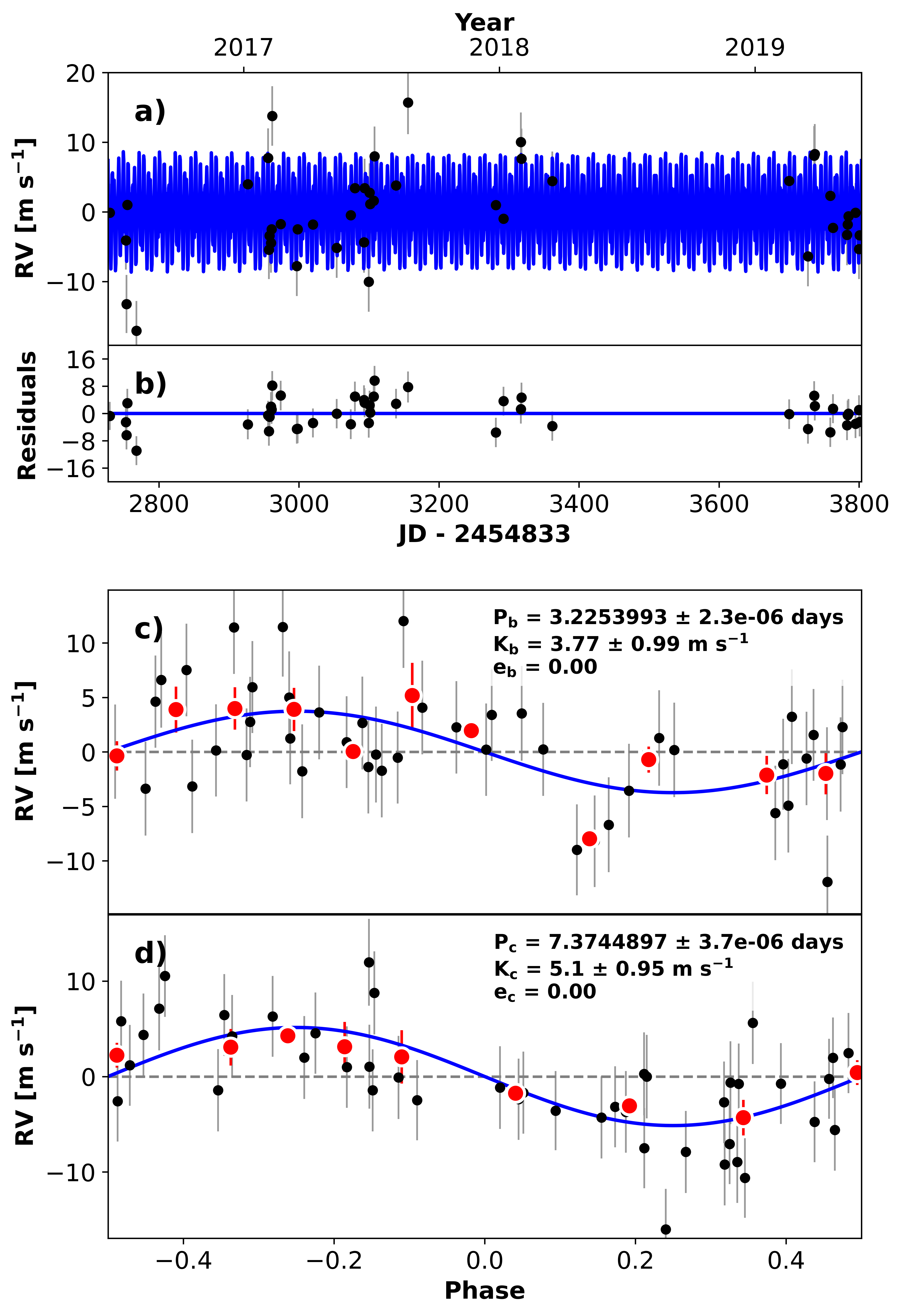
Figure 6: The best-fitting 2-planet Keplerian model for the K2-199 RVs. a) The MAP solution is the blue line, with Keck-HIRES RVs shown as the black points. Error bars represent pointwise RV measurement errors added in quadrature with an RV jitter term. b) Residuals about the best-fitting two-planet model. c) The phase-folded orbital solution for K2-199 b. Red points are data binned in units of 0.08 orbital phase. d) The same for K2-199 c.

K2-199 b and c were recently confirmed by Howard et al. (in prep) who modeled the K2 C6 photometry to derive planet ephemerides and used 33 Keck-HIRES RVs to measure $M_{\mathrm{b}}=7.8\pm 2.2$ $M_{\oplus}$ and $M_{\mathrm{c}}=11.0^{+2.7}_{-2.9}$ $M_{\oplus}$ for K2-182 b and c, respectively. Howard et al. (in prep) adopt a 2-planet, circular Keplerian model for the K2-199 RVs and suggest that extending the RV baseline will help determine the validity of a potential linear trend.

We explored several radvel models to fit the K2-199 RVs, all of which were 2-planet, circular Keplerian fits. In the end we choose a model that varies $P$, $T_{\mathrm{c}}$, and $K$ for each planet, fits a global RV jitter term, $\sigma_{j}$, and analytically calculates the RV instrumental offset, $\gamma_{j}$. We found that allowing $\gamma_{j}$ to vary during the MCMC produced near-identical results but slightly increased the model AICc ($\Delta\mathrm{AICc}<2$). Similar to K2-182 RV Model A, we impose a prior to keep $K>0$ for both planets, however a fit without the prior produced entirely similar results and did not bias the planet masses towards higher values. We elect to include the prior in our final solution because it is physically motivated. We allowed the planet ephemerides to vary within the tight priors from the K2 photometry because of the time difference between the end of K2 C17 and the start of our new RV observations (about 10 months). We would have done the same for K2-182 RV Model A if not for the small size of the data set. Model parameters, priors, and posterior estimates are summarized in Table 5. We improve the RV detection significance of both planets, especially K2-199 c, whose mass is now constrained to better than 5-$\sigma$ precision.

As we discussed in §4.2.2, we forgo a model of the K2-199 RVs that includes a GP trained on either the K2 photometry or the Keck-HIRES $S_{\text{HK}}$ values because of the significant change in spot behavior between the two K2 campaigns and the lack of periodicity in the $S_{\text{HK}}$ time series. Though by eye it seems like there may be slight correlation in the residuals in Figure 6, a periodogram of the RVs with the two Keplerians removed shows no peaks above the 0.01% false alarm probability level.

In addition to improving the planet mass determinations, our other main contribution to this system is in extending the RV observing baseline—our observations extend the baseline by more than a year when added to the Howard et al. (in prep) data set. We checked for a potential linear trend as mentioned by Howard et al. (in prep) but found no evidence for one. Our final mass measurements for K2-199 b and c are listed in Table 1.

Figure 7: The mass-radius diagram in the sub-Neptune regime. Data was compiled from the NASA Exoplanet Archive on 2020 Nov 20. We only include planets with better than 15% fractional measurement precision in radius and 33% fractional precision in mass. We note that the sample of planets shown here may lack completeness for low-density sub-Neptunes due to our fractional precision requirements, but they should not impact completeness at high-density (Burt et al., 2018; Montet, 2018; Teske et al., 2021). Planets and their 1-$\sigma$ measurement uncertainties are colored by equilibrium temperature assuming zero Bond albedo. Underlying contours from Gaussian kernel density estimation correspond to equal levels of fractional population in the mass-radius plane. We plot various density profiles to demonstrate that the sub-Neptune regime is host to numerous degeneracies in planet bulk composition. Dash-dot curves represent planets with Earth-like rock/iron cores surrounded by either a 0.1% or 2% H₂ envelope by mass (Zeng et al., 2019). The green dashed curve refers to planets with Earth-like rock/iron cores surround by a 50% layer of H₂O by mass (Zeng et al., 2016). Other composition curves are taken from Zeng et al. (2016). We draw attention to a small but growing sample of “super-dense” sub-Neptunes ($R_{\mathrm{p}}$ $<3$ $R_{\oplus}$ and $M_{\mathrm{p}}$ $>20$ $M_{\oplus}$), of which K2-182 b is a member. Others include two planets with masses from transit timing variations, Kepler-145 b (Xie, 2014) and Kepler-411 b (Sun et al., 2019), and three radial velocity confirmations, K2-66 b (Sinukoff et al., 2017), K2-292 b (Luque et al., 2019), and HD 21749 b (Gan et al., 2021). We discuss these super-dense sub-Neptunes further in §5.2.

5 Discussion

Our discussion is broken into three parts: First, in §5.1 we place K2-182 b and K2-199 b and c on the mass-radius diagram and compare their physical parameters to models of interior composition. In §5.2, we use K2-182 b as a launching point to take a closer look at a seemingly emerging group of super-dense sub-Neptunes ($R_{\mathrm{p}}$ $<3$ $R_{\oplus}$, $M_{\mathrm{p}}$ $>20$ $M_{\oplus}$). We review the literature for five of these planets to determine whether or not their high mass measurements could be explained by untreated signatures of correlated stellar variability in radial velocity data. We follow with a discussion of possible formation and evolution mechanisms for these unusually dense planets. Finally, in §5.3 we return to K2-182 b and K2-199 b and c to assess their viability as targets for space-based spectroscopic observations.

5.1 Bulk composition

The growing sub-Neptune population spans a wide range of bulk densities on the mass-radius plane. Furthermore, it is located in a region where numerous theoretical models of planet interiors and volatile envelopes converge. Precise mass, radius, and instellation flux estimates are the first step in discriminating between these degenerate compositions.

To infer the bulk compositions of K2-182 b ($\rho_{\mathrm{b}}$ $=$ $5.6\pm 1.4$ g cm^-3), K2-199 b ($\rho_{\mathrm{b}}$ $=$ $7.2^{+2.1}_{-2.0}$ g cm^-3), K2-199 c ($\rho_{\mathrm{c}}$ $=$ $2.9^{+0.7}_{-0.6}$ g cm^-3), we first compared their locations on the mass-radius plane with bulk density profiles from Zeng et al. (2016, 2019). Figure 7 shows the planets in the mass-radius diagram along with a sample of confirmed planets and various composition curves. By eye, the composition curves suggest that K2-182 b may have a significant core H₂O mass fraction, K2-199 b is likely rocky, and K2-199 c may have a substantial ($\gtrsim 1.5-2\%$ by mass) H₂-dominated envelope.

Figure 8: Joint and marginalized posteriors for our inference of $f_{H_{2}O}$ for the three planets, assuming a bulk composition of water and rock. Posterior median values and 68% confidence intervals are labeled at the top of each panel. Vertical dashed lines represent the median and bounds of the 68% confidence interval. K2-182 b’s mass and radius are consistent with a substantial core H₂O mass fraction. This may have implications for its formation mechanism, as discussed at the end of §5.2.8.

To make more quantitative statements about the possible bulk compositions of these planets, we compared our derived planet parameters to theoretical grids of interior composition. First, we used the grid from Zeng et al. (2016) to infer planet core water mass fractions ($f_{H_{2}O}$) assuming a two-component bulk composition of water and rock. We did this using the the Structure Model INTerpolator tool (smint; Piaulet et al. 2021), which performs linear interpolation on the grid of possible $f_{H_{2}O}$ and planet mass ($M_{\mathrm{p}}$) values to find the combination that best fits the measured planet radius.

We explored the posteriors of the inferred $f_{H_{2}O}$ and $M_{\mathrm{p}}$ values for each planet with emcee. We used an informed Gaussian prior on $M_{\mathrm{p}}$ stemming from our results in Table 1 and a uniform prior on $f_{H_{2}O}$ between 0 and 100%. We ran the MCMC with 100 chains for at least 20,000 steps each, discarding the first 60% of steps in each chain as burn-in. To ensure convergence, we continued sampling until each chain had run for at least 50 times the maximum autocorrelation time ($\tau$) across all parameters. In addition, we enforced that the maximum relative change in $\tau$ between convergence checks (every 1000 steps) was less than 1%. Finally, we visually inspected the chains to confirm a stationary and common distribution for each parameter. For each planet, the smint results for our interpolation on the Zeng et al. (2016) grid are shown in Figure 8 and summarized in Table 1. We find that K2-182 b’s mass and radius is consistent with a substantial water mass fraction of $f_{H_{2}O}$ $=$ $45^{+26}_{-20}$%. We infer small ($14^{+25}_{-11}$%) and large ($88^{+8}_{-14}$%) core water mass fractions for K2-199 b and c, respectively.

For K2-199 b and c we also used smint to infer the fraction of their mass that might be contained in a H₂/He envelope, assuming an Earth-like core of rock/iron, according to the grids of thermal evolution from Lopez & Fortney (2014). We do not infer $f_{\mathrm{env}}$ for K2-182 b because at 20 $M_{\oplus}$ it lies at the edge of the grid—though this is not to say that an ice-rich core is more likely for this planet than an Earth-like one (Owen & Wu, 2017). The analysis operated in an analogous way to our interpolation on the Zeng et al. (2016) grid, though the parameters in the fit were now the H₂/He envelope mass fraction ($f_{\mathrm{env}}$), $M_{\mathrm{p}}$, system age, and planet instellation flux ($S_{\mathrm{p}}$). smint interpolated on the Lopez & Fortney (2014) grids to find the values of these parameters that best matched the planet radius. The posterior estimation was similar to our method for $f_{H_{2}O}$. We used Gaussian priors on $M_{\mathrm{p}}$ and $S_{\mathrm{p}}$ for each planet using the values in Table 1. We placed uniform priors on $f_{\mathrm{env}}$ from 0.1 to 20% (the bounds of the Lopez & Fortney 2014 grid) and on the system age from 1 to 10 Gyr. Our results for K2-199 b and c are shown in Figure 9 and summarized in Table 1. K2-199 b’s mass, radius, and instellation flux are consistent with a very small H₂/He envelope ($f_{\mathrm{env}}$ $\leq 0.15$% at 3-$\sigma$ confidence), potentially indicative of photoevaporation. K2-199 c’s physical parameters are consistent with a larger H₂/He envelope mass fraction, $f_{\mathrm{env}}$ $=$ $2.9\pm 0.6$%.

Figure 7 also shows models of bulk interior composition from Zeng et al. (2019) corresponding to Earth-like rock/iron cores surrounded by an H₂-dominated envelope. We show the Zeng et al. (2019) models in Figure 7 for consistency with the Zeng et al. (2016) models. However, we choose to use the Lopez & Fortney (2014) grid to infer $f_{\mathrm{env}}$ rather than Zeng et al. (2019) because the former results from a study of thermal evolution, allowing us to marginalize over the age of the system.

5.2 Super-dense sub-Neptunes

K2-182 b’s mass measurement makes it one of the densest sub-Neptunes known to date. However, RV models of small planets around spotted stars can be greatly influenced by the in- or exclusion of GPs meant to account for stellar activity (Rajpaul et al., 2015; Faria et al., 2016; Dumusque et al., 2017; Jones et al., 2017; Rajpaul et al., 2017). While we found that our mass measurement for K2-182 b was consistent between RV models with and without a GP trained on the K2 photometry, we suggest that additional monitoring will better inform the influence of stellar activity on the spectroscopic observations. Furthermore, cases where star spots contribute to planet RV amplitude may be subject to publication bias because the inflated signal can more easily overcome standard fractional precision thresholds, like $M_{\mathrm{p}}$ $/\sigma_{M_{\mathrm{p}}}\geq 5$ (Burt et al., 2018; Montet, 2018; Batalha et al., 2019; Teske et al., 2021).

Here we review the literature for the handful of other “super-dense” sub-Neptunes ($R_{\mathrm{p}}$ $<3$ $R_{\oplus}$, $M_{\mathrm{p}}$ $>20$ $M_{\oplus}$) and question whether or not their high masses can be explained by unmitigated stellar activity. For a summary and general takeaways, see §5.2.7.

5.2.1 Sample and caveats

From our sample of confirmed planets shown in Figure 7, there are five sub-Neptunes other than K2-182 b that we consider “super-dense”: Kepler-145 b (Xie, 2014), Kepler-411 b (Sun et al., 2019), K2-66 b (Sinukoff et al., 2017), K2-292 b (Luque et al., 2019), and HD 21749 b (GJ 143 b; TOI-186.01; Trifonov et al. 2019; Dragomir et al. 2019; Gan et al. 2021). The masses of Kepler-145 b and Kepler-411 b were measured using transit timing variations (TTVs) and the remaining three are radial velocity confirmations. While our RV/stellar activity discussion does not apply to TTV measurements, we briefly summarize the physical parameters of Kepler-145 b and Kepler-411 b to add context to the super-dense sub-Neptunes as a whole.

For the purpose of our discussion, we chose to highlight these five planets because they are similar in mass and radius to K2-182 b. We acknowledge that they may not comprise a complete sample and the $R_{\mathrm{p}}$ $<3$ $R_{\oplus}$, $M_{\mathrm{p}}$ $>20$ $M_{\oplus}$ limits are a bit arbitrary. For example, we do not discuss the ultra-short period (USP) exposed planetary core orbiting the late-G dwarf, TOI-849 ($P=0.76$ days, $R_{\mathrm{p}}$ $=3.45$ $R_{\oplus}$, $M_{\mathrm{p}}$ $=40.8$ $M_{\oplus}$, $\rho_{\mathrm{p}}=5.5$ g cm^-3; Armstrong et al. 2020)—stellar activity signals due to star spots (timescales of several to tens of days for F, G, and K dwarfs) are unlikely to confuse the mass measurements of USPs ($P<1$ day), so we do not expect the RV mass of TOI-849 b to be biased due to stellar activity. Similarly, we do not include K2-110 b ($P=13.9$ days, $R_{\mathrm{p}}$ $=2.59$ $R_{\oplus}$, $M_{\mathrm{p}}$ $=16.7$ $M_{\oplus}$, $\rho=5.2$ g cm^-3), a dense sub-Neptune around a metal-poor ([Fe/H] $=-0.34\pm 0.03$ dex) K3V dwarf (Osborn et al., 2017). The K2-110 b authors note spot variations on the order of weeks are seen in the K2 light curve, meaning that the stellar rotation period (or one of its harmonics) could be in the neighborhood of the planet’s longer orbital period. Their $v\sin i$ measurement implies $\mathrm{Min}(P_{\mathrm{rot}})>9.2$ days, so further investigation may be warranted.

5.2.2 Kepler-145 b

Kepler-145 ($T_{\mathrm{eff}}$ $=6110\pm 122$ K, Berger et al. 2018) hosts two transiting planets confirmed by Xie (2014). Kepler-145 b ($P=22.9$ days) has $R_{\mathrm{p}}$ $=2.65\pm 0.08$ $R_{\oplus}$, $M_{\mathrm{p}}$ $=37.1\pm 11.6$ $M_{\oplus}$, and $\rho=10.9\pm 3.6$ g cm^-3, potentially making it the densest of all the super-dense sub-Neptunes we consider. However, when Otegi et al. (2020a) curated a high-fidelity sample of exoplanet mass and radius measurements from the NASA Exoplanet Archive, they excluded all planets from Xie (2014) because the masses disagree significantly with those from Hadden & Lithwick (2014, 2017). Furthermore, Kepler-145 b was not included in the broad sample of planets with secure TTV signals in either Hadden & Lithwick (2014) or Hadden & Lithwick (2017), making its mass even more suspect.

5.2.3 Kepler-411 b

Kepler-411 is an active K2V dwarf hosting four planets whose masses were measured by Sun et al. (2019) with TTVs. Kepler-411 b ($P=3.0$ days) is a hot ($T_{\mathrm{eq}}=1138$ K) sub-Neptune with $R_{\mathrm{p}}$ $=2.40\pm 0.05$ $R_{\oplus}$, $M_{\mathrm{p}}$ $=25.6\pm 2.6$ $M_{\oplus}$, and $\rho=10.3\pm 1.3$ g cm^-3. For reference, Otegi et al. (2020a) do include masses from Sun et al. (2019) in their revised exoplanet mass and radius catalog.

Figure 9: Joint and marginalized posteriors from our inference of $f_{\mathrm{env}}$ for K2-199 b and c are shown in blue (gray) assuming a 1$\times$ (50$\times$) solar metallicity H₂/He envelope on top of an Earth-like rock/iron core. Posterior median values and 68% confidence intervals for the $1\times$ solar metallicity case are labeled at the top of each panel.

5.2.4 K2-66 b

K2-66 (EPIC 206153219) is a relatively quiet ($\log R^{\prime}_{\mathrm{HK}}$ $=-5.27$ dex) G1 subgiant ($M_{*}$ $=1.11$ $M_{\odot}$, $R_{*}$ $=1.67$ $R_{\odot}$) with a transiting planet in the hot sub-Neptune desert (K2-66 b; $P=5.0$ days, $R_{\mathrm{p}}$ $=2.49^{+0.34}_{-0.24}$ $R_{\oplus}$, $T_{\mathrm{eq}}=1372\pm 51$ K; Sinukoff et al. 2017; Lundkvist et al. 2016). Sinukoff et al. (2017) confirm the planetary nature of K2-66 b using 38 precision RV measurements from Keck-HIRES, finding the planet is $M_{\mathrm{p}}$ $=21.3\pm 3.6$ $M_{\oplus}$ and $\rho=7.8\pm 2.7$ g cm^-3.

After extracting the K2 C3 EVEREST light curve in a similar way to our procedure in §2.2, we find that K2-66 shows long-term spot evolution ($\sim 50$ days) but no obvious rotation signatures closer to the time scale of K2-66 b’s orbital period. Using our adaptation of Equation 2 from Vanderburg et al. (2016) as in §4.2, we find that $\sigma_{\mathrm{phot}}=0.00075$ in units of relative flux (about an order of magnitude smaller than for K2-182 and K2-199). Combined with $v\sin i=3.7$ km s^-1 from the confirmation paper, $\sigma_{\mathrm{RV,\>spot}}\approx 2.8$ m s^-1 for K2-66 (a little more than 0.5$\times$ our upper limits on $\sigma_{\mathrm{RV,\>spot}}$ for K2-182 and K2-199).

Sinukoff et al. (2017) use a variety of radvel models to explain their RV measurements, settling on a 1-planet circular Keplerian fit. They do not find any significant peaks in a periodogram of the RV residuals after removing the signal for K2-66 b. With the star’s low magnetic activity and without clear signs of a stellar rotation period in the K2 C3 light curve, it seems that including a GP in a model of the RVs would not greatly affect the mass measurement. Keck-HIRES RV monitoring for this system in ongoing (Howard et al. in prep).

5.2.5 K2-292 b

Luque et al. (2019) confirm K2-292 b ($P=17.0$ days) using 18 precision RVs from the Calar Alto high-Resolution search for M dwarfs with Exoearths with Near-infrared and optical Échelle Spectrographs instrument (CARMENES; Quirrenbach et al. 2014, 2018) on the 3.5-m telescope at the Calar Alto Observatory in Spain. K2-292 (EPIC 212628254, HD 119130) is a G3V dwarf (Houk & Swift, 1999) observed in K2 C17. Through a joint analysis of the K2 photometry and CARMENES RVs, Luque et al. (2019) find $R_{\mathrm{p}}$ $=2.63^{+0.11}_{-0.10}$ $R_{\oplus}$, $M_{\mathrm{p}}$ $=24.5\pm 4.4$ $M_{\oplus}$, and $\rho=7.4^{+1.6}_{-1.5}$ g cm^-3. They also detect a linear trend in the RVs that could represent an outer companion with a minimum mass of $\sim 33$ $M_{\oplus}$. The authors suggest that additional data is required to rule out the possibilities that the trend is caused by stellar rotation or instrumental systematics.

The K2 C17 EVEREST light curve does not show significant spot modulation like those of K2-182 and K2-199. Repeating the process we carried out for K2-66, we find that $\sigma_{\mathrm{phot}}=0.00079$ in units of relative flux. The confirmation paper finds $v\sin i=4.6$ km s^-1, yielding $\sigma_{\mathrm{RV,\>spot}}\approx 3.6$ m s^-1. Luque et al. (2019) check for periodic signals in various stellar indices measured simultaneously with their RVs but find no evidence for correlated stellar activity, save for a peak in the H-$\alpha$ indices and the cross-correlation function FWHM at $P\sim 3.5$ days. Though additional RV observations could help constrain the nature of the potentially non-transiting outer companion, without clear evidence of spot modulation from the K2 photometry it does not seem like K2-292 warrants a GP-based analysis of its RVs.

5.2.6 HD 21749 b (GJ 143 b; TOI-186.01)

HD 21749 is a bright ($V=8.1$ mag) K4.5 dwarf. With multi-sector TESS photometry, Dragomir et al. (2019, hereafter D19b) discovered HD 21749 hosts a sub-Neptune (HD 21749 b; $P=35.6$ days, $R_{\mathrm{p}}$ $=2.61^{+0.17}_{-0.16}$ $R_{\oplus}$) and an Earth-size planet (HD 21749 c; $P=7.8$ days, $R_{\mathrm{p}}$ $=0.892^{+0.064}_{-0.058}$ $R_{\oplus}$).

Previously, Trifonov et al. (2019) had identified HD 21749 b as a single-transit planet candidate from the TESS Sector 1 and 2 photometry, and used a total of 58 publicly-available archival RVs from the High-Accuracy Radial-velocity Planet Searcher (HARPS; Mayor et al. 2003) instrument, mounted on the European Southern Observatory 3.6-m telescope at La Silla Observatory in Chile, to constrain the orbital period and measure the mass of planet b. Using the HARPS data, Trifonov et al. (2019) recover the orbital period and measure $M_{\mathrm{p}}$ $=30.63^{+2.63}_{-2.67}$ $M_{\oplus}$ by modeling the RVs with a moderately eccentric Keplerian orbit ($e=0.325^{+0.079}_{-0.079}$). They do not include HD 21749 c in a model of the RVs.

A few months after Trifonov et al. (2019) was published, D19b combined the HARPS RVs with archival ($N=48$) and newly-acquired ($N=34$) velocities from the Planet Finder Spectrograph (PFS; Crane et al. 2010) on the 6.5-m Magellan II Telescope at Las Campanas Observatory in Chile. This was in addition to two more sectors of TESS photometry which confirmed the orbital period of planet b at $P=35.6$ days. D19b jointly model the TESS photometry with the HARPS and PFS RVs, finding HD 21749 b is $M_{\mathrm{p}}$ $=22.7^{+2.2}_{-1.9}$ $M_{\oplus}$ and $\rho=7.0^{+1.6}_{-1.3}$ g cm^-3, and placing an upper limit on the mass of planet c. The Trifonov et al. (2019) mass is in near-3-$\sigma$ disagreement with the measurement from D19b. The D19b orbital solution also employs slightly smaller eccentricity for planet b, with $e=0.188^{+0.076}_{-0.078}$, and prefers a linear trend over the span of the $\sim 15$-year RV baseline. In the following, we discuss the results and methods from D19b rather than Trifonov et al. (2019) because the former was able to confirm the orbital period of planet b with TESS photometry before fitting their (larger) RV time series.

The TESS photometry of HD 21749 shows clear spot modulation with a peak-to-peak amplitude of about four parts per thousand in relative flux. D19b use stellar activity indices derived from their HARPS and PFS spectra along with long-term photometric monitoring from the Kilodegree Extremely Little Telescope (KELT; Pepper et al. 2004) to determine that the stellar rotation period is around 37 to 39 days, just longward of the period for planet b. Notably, while periodograms of the activity indices and photometry have peaks in this range, the same peaks do not manifest themselves in a periodogram of the RVs above the 0.01% FAP level (D19b Figure 5). The authors calculate $\sigma_{\mathrm{RV,\>spot}}\approx 1.3$ m s^-1 and suggest that uncertainties for their mass measurement may be slightly underestimated.

HD 21749 represents an interesting case where the stellar rotation period is likely very close (delta of a $\sim$few days) to the orbital period of the super-dense sub-Neptune. Though the rotation signals from the activity indicators and KELT photometry do not appear in the RV periodogram, a model of the RVs that includes a GP trained on the complementary data would provide a useful sanity check for the mass measurement of HD 21749 b. As a bright system with ample archival photometry and activity indicator measurements, HD 21749 is particularly amenable to a GP-based analysis.

Recently, Gan et al. (2021, hereafter G21) performed a more detailed accounting of stellar activity when they re-analyzed the HD 21749 system using the multi-sector TESS photometry and the HARPS $+$ PFS velocities from D19b, as well as 147 additional PFS observations. Using an updated TESS dilution factor, G21 find the radii of the two planets are slightly larger than reported in D19b. They also use a (slightly eccentric, $e_{\mathrm{b}}=0.164^{+0.062}_{-0.058}$) Keplerian $+$ GP model of the RVs to account for stellar rotation (the periodic hyperparameter of their GP kernel finds $P_{\mathrm{rot}}=34.1^{+2.4}_{-2.7}$ days). The resulting parameters they report for HD 21749 b are $R_{\mathrm{p}}$ $=2.86\pm 0.20$ $R_{\oplus}$, $M_{\mathrm{p}}$ $=20.0\pm 2.7$ $M_{\oplus}$, and $\rho=4.7^{+1.9}_{-1.4}$ g cm^-3. The mass measurements for HD 21749 b from D19b and G21 overlap within 1-$\sigma$, and the more intermediate bulk density of the planet owes primarily to the increase in its radius measurement—had the radius remained the same, when combined with the $M_{\mathrm{p}}$ $=20$ $M_{\oplus}$ measurement from G21 the bulk density would be $\sim$6.2 g cm^-3.

Comparing the D19b and G21 results, it does not appear that a stellar activity signal in the RV data set (though present) greatly affected the mass measurement of HD 21749 b in the D19b analysis. To conduct our own test of the hypothesis that unmitigated stellar activity may be artificially inflating the mass measurements of the super-dense sub-Neptunes, we re-analyzed the RVs from D19b with our own radvel models. The details of the analysis are described in Appendix C, but the GP training process largely follows the methodology in §4.2. For the sake of comparison with the Keplerian-only model of the RVs from D19b, we restricted our analysis to use only the velocities included in D19b rather than use the larger data set from G21.

We compared a variety of models of the HD 21749 RVs using the AICc, finding strong preference for models that included a GP component over ones without (generally $\Delta$AICc $>30$). Figure 10 compares a model of the RVs that attempts to replicate the solution in D19b (HD 21749 RV Model A) and one that differs only in the inclusion of a GP trained on the HARPS and PFS H-$\alpha$ indices (HD 21749 RV Model B). The HD 21749 b mass measurement from HD 21749 RV Model B is in good agreement with the one from Model A, and both agree with the results from D19b, further ameliorating concerns that the measurement is artificially inflated due to unmitigated stellar activity. Our mass measurements, though slightly larger, also overlap within 1-$\sigma$ with the result from G21. While not explicitly the same, the quasi-periodic GP kernel we employ is similar in effect to the kernel used in G21 (both represent a combination of exponentially-decaying and periodic signals).

5.2.7 Literature review summary

We briefly reviewed the confirmation papers for five super-dense sub-Neptunes, Kepler-145 b, Kepler-411 b, K2-66 b, K2-292 b, and HD 21749 b, to determine if unmitigated stellar activity signatures in RVs could have inflated the mass measurements of these planets. Though our activity discussion does not apply to TTV measurements, based on the concerns raised by Otegi et al. (2020a) Kepler-145 b’s TTV mass measurement from Xie (2014) should be handled with caution—we do not include it in the discussion below. Kepler-411 is an active K2V dwarf but masses in the system were also measured with TTVs so, again, our RV/activity discussion does not apply. EVEREST light curves do not show clear signs of spot modulation for the G1 subgiant K2-66 or the solar-like G3V dwarf K2-292. These systems do not seem to warrant an RV model that includes a GP.

HD 21749 is a spotted K4.5 dwarf with a rotation period that is likely close to the orbital period of planet b. D19b offer a thorough investigation into possible signatures of stellar activity in the RVs, finding little sign of the stellar rotation period in their extensive ($N=141$) RV time series. G21 provide a more detailed accounting of stellar activity in the HD 21749 RVs, adding 147 PFS observations to the D19b data set and including a GP in a model of the velocities. Their mass measurement of HD 21749 b, though slightly smaller, overlaps with the result from D19b within 1-$\sigma$. The more intermediate density G21 report for planet b is primarily due to their larger planet radius measurement, which results from an updated TESS dilution factor. As another sanity check, we modeled the HD 21749 RVs as a combination of Keplerians and a GP, restricting ourselves to the D19b data set to create a more direct comparison between their Keplerian-only model. We find that while a model of the RVs which includes a GP trained on activity indicators is strongly preferred by the AICc and produces smaller scatter in the residuals (see Figure 10), its mass measurement for HD 21749 b is entirely consistent with a model that does not include the GP (and both models are consistent with the D19b and G21 results). Though the mass measurement of HD 21749 b from G21 is slightly smaller than reported in D19b and this work, it does not seem to indicate that untreated stellar activity was greatly impacting the planet mass measurement. Having found no compelling evidence that stellar activity is producing inflated RV mass measurements for these planets, we are confident that this is a growing, bonafide population of super-dense sub-Neptunes.

5.2.8 Super-dense sub-Neptune formation and evolution

Several explanations have been posited as the formation and/or evolution mechanism(s) behind the super-dense sub-Neptunes. These include photoevaporation, migration, and giant impacts. Here we briefly discuss how these scenarios relate to our sample and revisit K2-182 b.

In the case of the highly-irradiated K2-66 b ($S_{\mathrm{p}}\approx 840$ $S_{\oplus}$), the planet was probably stripped of its primordial atmosphere through photoevaporation as K2-66 evolved off of the main sequence. With $S_{\mathrm{p}}\approx 220$ $S_{\oplus}$, it seems that photoevaporation could also have a hand in the density of Kepler-411 b. However the system is relatively young with a gyrochronological age of $212\pm 31$ Myr (Sun et al., 2019). Using Equation 15 from Lecavelier Des Etangs (2007), we find that with $a=0.038$ AU, Kepler-411 b would only lose 0.01 $M_{\oplus}$ due to extreme ultraviolet radiation (EUV) from its K2V host over the system’s gyrochronological age. Otegi et al. (2020a) suggest that Kepler-411 b could be ice-rich and represent the maximum allowed core mass, in line with models of Saturn and Jupiter’s interiors, which infer core masses up to 20 and 25 $M_{\oplus}$, respectively (Saumon & Guillot, 2004; Wahl et al., 2017).

Luque et al. (2019) show that K2-292 b receives too little instellation ($S_{\mathrm{p}}\approx 67$ $S_{\oplus}$) for its density to be explained by EUV-driven photoevaporation. Instead, following an explanation similar to the one for K2-110 b (Osborn et al., 2017), Luque et al. (2019) propose that K2-292 b was formed at high density. In situ formation is ruled out, as the required disk mass enhancement factor to the minimum-mass solar nebula (MMSN) is greater than 40 (Schlichting, 2014). Rather, Luque et al. (2019) suggest K2-292 b could have formed beyond the snow line and migrated inward due to Kozai-Lidov oscillations (Kozai, 1962; Lidov, 1962; Dawson & Chiang, 2014; Mustill et al., 2017) excited by an outer companion (possibly the linear trend they detect in the RVs).

HD 21749 b is the coolest super-dense sub-Neptune ($T_{\mathrm{eq}}=407^{+22}_{-19}$ K from G21) meaning that photoevaporation is not a viable explanation. Given its moderate orbital eccentricity ($e=0.164^{+0.062}_{-0.058}$ from G21), the presence of the close-in Earth-size HD 21749 c, and the possibility of an outer companion due to the linear trend in the D19b RVs (though no trend is found in the G21 data set), HD 21749 b could have also formed beyond the snow line and migrated to its present location ($a=0.21$ AU from G21) due to dynamical interactions.

Returning to K2-182 b, we first tried to place an upper limit on its mass-loss rate due to EUV radiation. Using Equation 15 from Lecavelier Des Etangs (2007), we find K2-182 b could lose up to 0.5 $M_{\oplus}$ over 10 Gyr from EUV instellation, i.e. $2.5$% of its current mass. According to the grids from Lopez & Fortney (2014), if a planet with K2-182 b’s mass (20 $M_{\oplus}$) and radius (2.7 $R_{\oplus}$) and $S_{\mathrm{p}}=10$ $S_{\oplus}$ (instead of K2-182 b’s $\approx 150$ $S_{\oplus}$) were to lose all of a primordial 2% H₂/He envelope over 10 Gyr, this would correspond to a reduction in radius of $\sim 0.8$ $R_{\oplus}$. The radius reduction would be even more dramatic in the case of maximum EUV-driven mass-loss at K2-182 b’s actual instellation. It seems suspect that K2-182 ($L\approx 0.4$ $L_{\odot}$) could strip away 1 $R_{\oplus}$ from K2-182 b, so while photoevaporation may play a role in K2-182 b’s density, it does not appear to be the dominating factor.

To rule out formation in situ, using Equation 7 from Schlichting (2014) we calculated the required disk mass enhancement factor ($\mathcal{F}$) to the MMSN needed in order to form our 20 $M_{\oplus}$ planet at 0.05 AU. We find $\mathcal{F}>100$, implying that like K2-292 b, K2-182 b must have migrated to its current location from farther out ($>2$ AU) in the protoplanetary disk. However, the delivery of 50-100 $M_{\oplus}$ of rocky material to the inner disk combined with the constructive collisions of primordial icy cores could potentially provide an out for the in situ formation scenario (Hansen & Murray, 2012; Inamdar & Schlichting, 2015; Zeng et al., 2019). In situ formation via giant impacts is not viable for typical sub-Neptunes with $f_{\mathrm{env}}$ of a few percent because the impacts drive atmospheric mass-loss, but it could help explain the small envelope mass for planets like K2-182 b. Furthermore, our results from interpolation on the Zeng et al. (2016) grids show that K2-182 b’s mass and radius are consistent with a substantial core H₂O mass fraction (see Figure 8).

Similar to Kepler-411 b, if K2-182 b is the product of constructive collisions of icy cores, then it could represent the maximum allowed core mass. Otegi et al. (2020a) point out that models of giant planet formation via pebble accretion and migration predict pebble isolation masses on the order of 10 to 20 $M_{\oplus}$ (Johansen & Lambrechts, 2017; Bitsch et al., 2019), which is seemingly consistent with these $\sim$20-25 $M_{\oplus}$ super-dense sub-Neptunes. Therefore some combination of pebble accretion, giant impacts, and migration caused by interactions with a gaseous disk could explain K2-182 b’s formation.

Additional RV observations will shed light on K2-182 b’s dynamical history, helping to distinguish between the scenarios we have already mentioned and migration due to an interaction with an outer companion. RV follow-up could do this by checking for a linear trend in the velocities and/or better-constraining the orbital eccentricity, which is nominally small but slightly skewed (perhaps in-part due to Lucy-Sweeney bias) towards moderate values as measured from the K2 transits ($e=$ $0.04^{+0.19}_{-0.03}$).

In summary, save for K2-66 b, photoevaporation is unable to explain the super-dense sub-Neptune population—this should be unsurprising, given that the Fulton gap (Fulton et al., 2017) does not extend to $R_{\mathrm{p}}$ $\gtrsim 2$ $R_{\oplus}$. Migration probably played a roll in the formation and evolution of Kepler-411 b, K2-292 b, HD 21749 b, and K2-182 b. Extending K2-182 b’s RV baseline to check for an outer companion and moderate eccentricity could help distinguish between scenarios of in situ formation, pebble accretion plus migration due to planet-disk interactions, and migration from a dynamical interaction.

5.3 Prospects for the atmospheric characterization of K2-182 b and K2-199 b and c

For sub-Neptunes that lie between the Earth-like and pure H₂O composition curves (e.g. the super-dense sub-Neptunes), improvements to mass and radius measurement precision alone cannot break degeneracies between various planet core, mantle, water, and envelope mass fractions (Valencia et al., 2007; Otegi et al., 2020b). Instead, measurements of atmospheric metallicity via space-based transmission spectroscopy are needed to constrain models of interior structure. While massive planets with small volatile envelopes are unattractive targets for these studies because of their meager atmospheric scale heights, a better understanding of their composition could inform important questions in planet formation (Kite et al., 2020).

We used the transmission spectroscopy metric (TSM; Kempton et al. 2018) to quantify the expected SNR of a 10-hour observing program with JWST-NIRISS for K2-182 b, assuming a cloud-free, solar metallicity atmosphere:

$$\centering\mathrm{TSM}=(\textrm{scale factor})\times\frac{R_{\mathrm{p}}^{3}T_{\mathrm{eq}}}{M_{\mathrm{p}}R_{*}^{2}}\times 10^{-m_{J}/5}.\@add@centering$$ (16)

The “scale factor” is a dimensionless normalization constant equal to 1.26 for planets $1.5<R_{p}<2.75$ $R_{\oplus}$ (i.e. K2-182 b and K2-199 b) and 1.28 for planets $2.75<R_{p}<4.0$ $R_{\oplus}$ (i.e. K2-199 c).

K2-182 b’s TSM ($16^{+5}_{-3}$) is very low—Kempton et al. (2018) propose a cutoff of TSM $>92$ for planets between $1.5<R_{p}<2.75$ $R_{\oplus}$ to warrant space-based follow-up. K2-182 b’s TSM scales to an expected single-transit SNR of $8\pm 2$. HD 21749 b might serve as the best candidate for atmospheric observations of a super-dense sub-Neptune (see §5.1 in G21), though at $J=6.0$ mag HD 21749 is too bright for observations with JWST-NIRISS.

On the other hand, K2-199 is better-suited for atmospheric studies given K2-199 c’s intermediate density ($\rho=$ $2.9^{+0.7}_{-0.6}$ g cm^-3) and 5-$\sigma$-precision mass measurement (Batalha et al., 2019). Using Equation 16 we find K2-199 c has a TSM value of $32^{+9}_{-6}$, which scales to a single-transit SNR of $16\pm 4$. K2-199 b’s TSM value is low ($17^{+6}_{-4}$; single-transit SNR of $7\pm 2$), though as a multi-planet system, atmospheric observations of K2-199 b and c would be especially valuable to test theories of planet formation.

6 Conclusion

Using multi-campaign K2 photometry and precise RV measurements from Keck-HIRES, we measured the physical parameters of K2-182 b ($P=4.7$ days, $R_{\mathrm{p}}$ $=$ $2.69^{+0.07}_{-0.05}$ $R_{\oplus}$, $M_{\mathrm{p}}$ $=$ $20\pm 5$ $M_{\oplus}$), K2-199 b ($P=3.2$ days, $R_{\mathrm{p}}$ $=$ $1.73^{+0.05}_{-0.04}$ $R_{\oplus}$, $M_{\mathrm{p}}$ $=$ $6.9\pm 1.8$ $M_{\oplus}$), and K2-199 c ($P=7.4$ days, $R_{\mathrm{p}}$ $=$ $2.85^{+0.10}_{-0.09}$ $R_{\oplus}$, $M_{\mathrm{p}}$ $=$ $12.4\pm 2.3$ $M_{\oplus}$). In §2 we extracted the EVEREST light curves and modeled the two campaigns of K2 photometry for each system. Importantly, this resulted in significant improvements to the orbital ephemerides (Figure 3). In §3 we characterized K2-182 (an early-K dwarf) and K2-199 (a K5V dwarf) with high-resolution spectroscopy and imaging. In §4 we reported our RV observations, searched for signatures of stellar activity, and measured the planet masses. Our adopted RV solution for K2-182 is shown on the left in Figure 5. Our RV solution for K2-199 is shown in Figure 6. Measured and derived planet parameters are summarized in Table 1. We find that K2-182 b may be a “super-dense” sub-Neptune, with $R_{\mathrm{p}}$ $=$ $2.69^{+0.07}_{-0.05}$ $R_{\oplus}$ and $\rho=$ $5.6\pm 1.4$ g cm^-3, though additional RV monitoring is needed to more confidently place it among this group of unusually dense planets. For K2-199, we surpass the 5-$\sigma$ detection level for K2-199 c.

In §5.1 we inferred the bulk compositions of our three planets using theoretical models of planet interiors and thermal evolution. We find that K2-182 b’s mass and radius are consistent with an ice-rich core ($f_{H_{2}O}$ $=$ $45^{+26}_{-20}$%). Using the grids from Lopez & Fortney (2014), we find that K2-199 b has a very small H₂/He envelope mass fraction ($f_{\mathrm{env}}$ $=$ $0.03^{+0.04}_{-0.01}$%) meaning it is probably rocky, while K2-199 c has a more substantial envelope ($f_{\mathrm{env}}$ $=$ $2.9\pm 0.6$%).

In §5.2 we reviewed the literature of the “super-dense” sub-Neptunes ($R_{\mathrm{p}}$ $<3$ $R_{\oplus}$, $M_{\mathrm{p}}$ $>20$ $M_{\oplus}$; see Figure 7) to examine whether or not unmitigated stellar activity could have artificially inflated their high mass measurements. We conducted our own analysis of the HD 21749 RVs as reported by Dragomir et al. (2019) and found agreement in the mass measurement for the super-dense sub-Neptune HD 21749 b between a model of the RVs with and without a Gaussian process trained on stellar activity indicators. We also found agreement between our measurements and the results of Gan et al. (2021), which uses a larger RV data set in addition to a GP model of the stellar activity signal. Details and results of our analysis are found in Appendix C. While the mass measurements for HD 21749 b agree between our two models (and both agree with the results in Dragomir et al. 2019 and Gan et al. 2021) the GP-enabled model is heavily favored by the Akaike Information Criterion ($\Delta$AICc $>30$) and produces a lower RMS scatter in the residuals ($\Delta$RMS $>2.5$ m s^-1). Overall, we find no evidence that unmitigated stellar activity can explain the high mass measurements of the super-dense sub-Neptunes.

We discussed formation and evolution scenarios for these unusually dense planets, including K2-182 b, in §5.2.8. Save for K2-66 b, which lies in the hot sub-Neptune desert, it seems that photoevaporation cannot explain the masses and radii of the super-dense sub-Neptunes. Instead, formation via giant impacts or migration due to dynamical interactions with the gaseous protoplanetary disk or an outer companion likely occurred (or some combination thereof).

K2-182 b and K2-199 b and c are not enticing targets for atmospheric characterization with JWST according to the transmission spectroscopy metric from Kempton et al. (2018). However, we note that due to degeneracies in models of planet bulk composition, measurements of atmospheric metallicity may be the only way to shed light on the interiors and formation histories of super-dense sub-Neptunes like K2-182 b. In addition, as a multi-planet system with a precise ($>5$-$\sigma$) mass measurement for planet c, K2-199 is a valuable opportunity for atmospheric studies to probe models of planet formation.

ACKNOWLEDGMENTS

We thank the anonymous referee for their thorough reading of this work—their detailed comments improved the quality of the manuscript. J.M.A.M. is supported by the National Science Foundation Graduate Research Fellowship Program under Grant No. DGE-1842400. J.M.A.M. acknowledges the LSSTC Data Science Fellowship Program, which is funded by LSSTC, NSF Cybertraining Grant No. 1829740, the Brinson Foundation, and the Moore Foundation; his participation in the program has benefited this work. M.R.K. is supported by the NSF Graduate Research Fellowship, grant No. DGE 1339067. A.B. is supported by the NSF Graduate Research Fellowship, grant No. DGE 1745301. L.M.W. is supported by the Beatrice Watson Parrent Fellowship and NASA ADAP Grant 80NSSC19K0597.

We acknowledge use of the lux supercomputer at UC Santa Cruz, funded by NSF MRI grant AST 1828315. J.M.A.M. would like to thank Brant Robertson, Josh Sonstroem, and Ryan Hausen for their help with lux access and setup. J.M.A.M. would also like to thank Jonathan Fortney for sharing computational resources and Aarynn Carter for helpful conversations.

The authors wish to recognize and acknowledge the very significant cultural role and reverence that the summit of Mauna Kea has always had within the indigenous Hawaiian community. We are most fortunate to have the opportunity to conduct observations from this sacred mountain which is now colonized land.

Appendix A K2-182 and K2-199 photometric models

Here we include tables describing the parameters, priors, and posteriors for our photometric models of the K2-182 and K2-199 EVEREST light curves. In many cases, the actual values for the model parameters may not be of physical interest (most of the relevant physical planet parameters can be found in Table 1) but are listed here for completeness.

Table 2: K2-182 photometric model

Parameter	Symbol	Units	Prior	Posterior Median $\pm$ 1-$\sigma$	Notes
Light curve parameters
Light curve mean offset	$\mu$	ppt	$\mathcal{N}$(0, 10)	$-0.11^{+0.33}_{-0.31}$
Log photometric variance	$\log$ $\sigma^{2}_{\mathrm{phot}}$	$\log$ ppt2	$\mathcal{N}$($\log s^{2}_{\mathrm{phot}}$, 5)	$-5.139\pm 0.023$	A
Stellar parameters
Limb darkening parameter 1	$q_{1}$		$\mathcal{U}$[0, 1]	$0.48^{+0.28}_{-0.20}$	B
Limb darkening parameter 2	$q_{2}$		$\mathcal{U}$[0, 1]	$0.44^{+0.26}_{-0.16}$	B
Stellar mass	$M_{*}$	$M_{\odot}$	$\mathcal{N}$(0.86, 0.1)[0, 1.5]	$0.865\pm 0.017$	C
Stellar radius	$R_{*}$	$R_{\odot}$	$\mathcal{N}$(0.79, 0.1)[0, 1.5]	$0.794^{+0.012}_{-0.011}$	C
Planet parameters
Log orbital period	$\log P$	$\log$ days	$\mathcal{N}$($\log P_{\mathrm{L18}}$, 1)	$1.55539733\pm 0.00000048$	D
Time of inferior conjunction	$T_{\mathrm{c}}$	$\mathrm{BJD}-2454833$	$\mathcal{N}$($T_{\mathrm{c},\>\mathrm{L18}},1)$	$2886.11517\pm 0.00028$	D
Log planet radius	$\log$ $R_{\mathrm{p}}$	$\log$ $R_{\oplus}$	$\mathcal{N}$($\log R_{\mathrm{p}0}$, 1)	$0.991^{+0.027}_{-0.021}$	E
Impact parameter	$b$		$\mathcal{U}$[0, $1+\frac{R_{\mathrm{p}}}{R_{*}}$]	$0.20^{+0.19}_{-0.13}$	F
$\sqrt{e}\cos({\omega})$	$\xi_{1}$		$\mathcal{D}$($\xi_{1}$, $\xi_{2}$)[0, 1], VE($e|\bm{\theta}$)	$0.00\pm 0.25$
$\sqrt{e}\sin({\omega})$	$\xi_{2}$		$\mathcal{D}$($\xi_{1}$, $\xi_{2}$)[0, 1], VE($e|\bm{\theta}$)	$-0.06^{+0.13}_{-0.16}$
GP hyperparameters
GPdec log amplitude parameter	$\log S_{0\mathrm{,dec}}\omega_{0\mathrm{,dec}}^{4}$	log ppt2 rad3 days-3	$\mathcal{N}$($\log s^{2}_{\mathrm{phot}}(\frac{2\pi}{10})^{4}$, 5)	$1.80^{+0.56}_{-0.61}$	G
GPdec log angular frequency	$\log\omega_{0\mathrm{,dec}}$	$\log$ rad days-1	$\mathcal{N}$($\log\frac{2\pi}{10}$, 5)	$2.90^{+0.19}_{-0.21}$
GPdec quality factor	$Q_{\mathrm{dec}}$		fixed	$\equiv\frac{1}{\sqrt{2}}$	H
GProt log amplitude	$\log S_{0\mathrm{,rot}}$	$\log$ ppt2 rad-1 days	$\mathcal{N}$($\log s^{2}_{\mathrm{phot}}$, 5)	$2.32^{+0.54}_{-0.45}$
GProt log period	$\log P_{\mathrm{rot}}$	$\log$ days	$\mathcal{N}$($\log$ 24.82, 5)[0, 50]	$3.211^{+0.051}_{-0.046}$	I
GProt log quality factor	$\log Q_{0\mathrm{,rot}}$		$\mathcal{N}$(1, 2)	$1.82^{+0.51}_{-0.44}$	J
GProt log quality factor separation	$\log\delta Q_{0\mathrm{,rot}}$		$\mathcal{N}$(1, 2)	$0.5^{+1.5}_{-1.8}$	K
GProt mixture fraction	$f$		$\mathcal{U}$[0, 1]	$0.63^{+0.24}_{-0.26}$	L

Note. — “Log” refers to the natural logarithm. $\mathcal{N}$(X, Y) refers to a Gaussian distribution with mean X and standard deviation Y. $\mathcal{N}$(X, Y)[A, B] refers to a bounded Gaussian with mean X, standard deviation Y, and hard bounds at A and B. $\mathcal{U}$[X, Y] refers to a uniform distribution inclusive on the interval X and Y. $\mathcal{D}$($\xi_{1}$, $\xi_{2}$)[0, 1] refers to a uniform distribution over the unit disk (i.e. $\sqrt{\xi_{1}^{2}+\xi_{2}^{2}}\leq 1$). VE($e|\bm{\theta}$) refers to the mixture distribution from Van Eylen et al. (2019) which is used as a prior on $e$ and whose hyperparameters, $\bm{\theta}$, are marginalized over. GP_dec and GP_rot refer to the exponential decay and rotation terms of the GP kernel, respectively.

A: $\sigma_{\mathrm{phot}}$ is treated as a uniform point-wise flux measurement error. $s^{2}_{\mathrm{phot}}$ indicates the sample variance of the flux data.

B: The parameterization $q_{1}\equiv(u_{1}+u_{2})^{2}$ and $q_{2}\equiv 0.5u_{1}(u_{1}+u_{2})^{-1}$, where $u_{1}$ and $u_{2}$ are the usual quadratic limb darkening coefficients, follows the prescription by Kipping (2013) for efficient, uninformative sampling of $u_{1}$ and $u_{2}$.

C: The stellar mass and radius were given Gaussian priors according to the results from our analysis in §3.1, with hard bounds at 0 and 1.5 $M_{\odot}$ and $R_{\odot}$, respectively.

D: $P_{\mathrm{L18}}=4.7368$ days and $T_{\mathrm{c},\>\mathrm{L18}}=2308.20626$ BJD - 245833 are the orbital period and time of inferior conjunction for K2-182 b as reported by L18.

E: $\log R_{\mathrm{p}0}=\log\big{(}(\frac{R_{\mathrm{p}}}{R_{*}}_{L18})^{2}\times R_{*}\big{)}$ where $\frac{R_{\mathrm{p}}}{R_{*}}_{L18}=0.00317$ is the occultation fraction for K2-182 b as reported by L18 and $R_{*}=0.86$ $R_{\odot}$ is the stellar radius resulting from our analysis in §3.1.

F: The upper bound of the uniform prior on $b$ is conditional on the ratio of the (free) model parameters for planet and stellar radius.

G: The power of the GP_dec term (in units of ppt²) at $\omega_{\mathrm{GP}}=0$ is $\sqrt{\frac{2}{\pi}}S_{0\mathrm{,dec}}$. Our model fits the logarithm of $S_{0\mathrm{,dec}}\omega_{0\mathrm{,dec}}^{4}$ and calculates $S_{0\mathrm{,dec}}$ deterministically because $S_{0\mathrm{,dec}}$ and $\omega_{0\mathrm{,dec}}$, the angular frequency of the undamped oscillation, can show strong covariance.

H: A quality factor of $\frac{1}{\sqrt{2}}$ gives this stochastic damped harmonic oscillator the same power spectral density as stellar granulation (Harvey, 1985; Kallinger et al., 2014).

I: The center of the prior comes from a Lomb-Scargle periodogram (Lomb, 1976; Scargle, 1982) of the light curve.

J: $Q_{0\mathrm{,rot}}$ is the quality factor minus $\frac{1}{2}$ for the GP rotation term’s oscillator at $\frac{P_{\mathrm{rot}}}{2}$.

K: The difference between the quality factors of the oscillators at $P_{\mathrm{rot}}$ and $\frac{P_{\mathrm{rot}}}{2}$.

L: The fractional amplitude of the oscillator at $\frac{P_{\mathrm{rot}}}{2}$ relative to the one at $P_{\mathrm{rot}}$.

Table 3: K2-199 photometric model

Parameter	Symbol	Units	Prior	Posterior Median $\pm$ 1-$\sigma$
Light curve parameters
Light curve mean offset	$\mu$	ppt	$\mathcal{N}$(0, 10)	$0.3^{+1.5}_{-1.3}$
Log photometric variance	$\log$ $\sigma^{2}_{\mathrm{phot}}$	$\log$ ppt2	$\mathcal{N}$($\log s^{2}_{\mathrm{phot}}$, 5)	$-4.960\pm 0.022$
Stellar parameters
Limb darkening parameter 1	$q_{1}$		$\mathcal{U}$[0, 1]	$0.70^{+0.21}_{-0.25}$
Limb darkening parameter 2	$q_{2}$		$\mathcal{U}$[0, 1]	$0.31^{+0.18}_{-0.10}$
Stellar mass	$M_{*}$	$M_{\odot}$	$\mathcal{N}$(0.86, 0.1)[0, 1.5]	$0.713^{+0.022}_{-0.023}$
Stellar radius	$R_{*}$	$R_{\odot}$	$\mathcal{N}$(0.79, 0.1)[0, 1.5]	$0.680^{+0.014}_{-0.013}$
Planet b parameters
Log orbital period	$\log P$	$\log$ days	$\mathcal{N}$($\log P_{\mathrm{L18}}$, 1)	$1.17105674^{+0.00000073}_{-0.00000072}$
Time of inferior conjunction	$T_{\mathrm{c}}$	$\mathrm{BJD}-2454833$	$\mathcal{N}$($T_{\mathrm{c},\>\mathrm{L18}}$, 1)	$2385.73733^{+0.00051}_{-0.00055}$
Log planet radius	$\log$ $R_{\mathrm{p}}$	$\log$ $R_{\oplus}$	$\mathcal{N}$($\log R_{\mathrm{p}0}$, 1)	$0.552^{+0.032}_{-0.028}$
Impact parameter	$b$		$\mathcal{U}$[0, $1+\frac{R_{\mathrm{p}}}{R_{*}}$]	$0.25^{+0.12}_{-0.15}$
$\sqrt{e}\cos({\omega})$	$\xi_{1}$		$\mathcal{D}$($\xi_{1}$, $\xi_{2}$)[0, 1], VE($e|\bm{\theta}$)	$0.00\pm 0.15$
$\sqrt{e}\sin({\omega})$	$\xi_{2}$		$\mathcal{D}$($\xi_{1}$, $\xi_{2}$)[0, 1], VE($e|\bm{\theta}$)	$0.00\pm 0.16$
Planet c parameters
Log orbital period	$\log P$	$\log$ days	$\mathcal{N}$($\log P_{\mathrm{L18}}$, 1)	$1.99802670\pm 0.00000049$
Time of inferior conjunction	$T_{\mathrm{c}}$	$\mathrm{BJD}-2454833$	$\mathcal{N}$($T_{\mathrm{c},\>\mathrm{L18}}$, 1)	$2389.93034\pm 0.00035$
Log planet radius	$\log$ $R_{\mathrm{p}}$	$\log$ $R_{\oplus}$	$\mathcal{N}$($\log R_{\mathrm{p}0}$, 1)	$1.047^{+0.036}_{-0.032}$
Impact parameter	$b$		$\mathcal{U}$[0, $1+\frac{R_{\mathrm{p}}}{R_{*}}$]	$0.25^{+0.12}_{-0.15}$
$\sqrt{e}\cos({\omega})$	$\xi_{1}$		$\mathcal{D}$($\xi_{1}$, $\xi_{2}$)[0, 1], VE($e|\bm{\theta}$)	$0.01^{+0.12}_{-0.14}$
$\sqrt{e}\sin({\omega})$	$\xi_{2}$		$\mathcal{D}$($\xi_{1}$, $\xi_{2}$)[0, 1], VE($e|\bm{\theta}$)	$0.02\pm 0.16$
GP hyperparameters
GPdec log amplitude parameter	$\log S_{0\mathrm{,dec}}\omega_{0\mathrm{,dec}}^{4}$	log ppt2 rad3 days-3	$\mathcal{N}$($\log s^{2}_{\mathrm{phot}}(\frac{2\pi}{10})^{4}$, 5)	$-2.37^{+0.18}_{-0.26}$
GPdec log angular frequency	$\log\omega_{0\mathrm{,dec}}$	$\log$ rad days-1	$\mathcal{N}$($\log\frac{2\pi}{10}$, 5)	$-1.87^{+0.21}_{-0.27}$
GPdec quality factor	$Q_{\mathrm{dec}}$		fixed	$\equiv\frac{1}{\sqrt{2}}$
GProt log amplitude	$\log S_{0\mathrm{,rot}}$	$\log$ ppt2 rad-1 days	$\mathcal{N}$($\log s^{2}_{\mathrm{phot}}$, 5)	$0.79^{+0.67}_{-0.66}$
GProt log period	$\log P_{\mathrm{rot}}$	$\log$ days	$\mathcal{N}$($\log$ 15.36, $\log$ 5)[$\log$ 1, $\log$ 21]	$2.730^{+0.023}_{-0.025}$
GProt log quality factor	$\log Q_{0\mathrm{,rot}}$		$\mathcal{N}$(1, 2)	$-7.31^{+0.31}_{-0.30}$
GProt log quality factor separation	$\log\delta Q_{0\mathrm{,rot}}$		$\mathcal{N}$(1, 2)	$3.40^{+1.21}_{-1.12}$
GProt mixture fraction	$f$		$\mathcal{U}$[0, 1]	$0.001^{+0.001}_{-0.000}$

Note. — Notation and parameters are analogous to Table 2. We include a tight prior on $\log P_{\mathrm{rot}}$ because in using a wide prior similar to the one in our model of K2-182, we found the marginal posterior was multimodal and caused sampling performance to suffer. The multimodality is probably a symptom of the stark difference in behavior between the K2 C6 and C17 light curves of K2-199, seen in the top panel of Figure 2. Therefore, for K2-199 $\log P_{\mathrm{rot}}$ should not be thought of as a robust estimate of the stellar rotation period and only as a non-physical model parameter used to flatten the light curve.

Appendix B K2-182 and K2-199 radial velocity models

Here we include tables describing the parameters, priors, and posteriors for our models of the K2-182 and K2-199 Keck-HIRES RVs. Derived parameters are summarized in Table 1. We also include tables with our Keck-HIRES RV measurements.

Table 4: K2-182 RV models

Parameter	Symbol	Units	Prior	Posterior Median $\pm$ 1-$\sigma$
K2-182 RV Model A (1-planet circular Keplerian; adopted)
Planet b orbital parameters
Orbital period	$P$	days	fixed	$\equiv 4.7369683$
Time of inferior conjunction	$T_{\mathrm{c}}$	BJD - 2454833	fixed	$\equiv 2886.11517$
Orbital eccentricity	$e$		fixed	$\equiv 0$
Argument of periastron	$\omega$	rad	fixed	$\equiv 0$
RV semi-amplitude	$K$	m s-1	$K>0$	$8.4\pm 2.0$
Instrument parameters
HIRES RV offset	$\gamma_{j}$	m s-1	fixed	$\equiv-2.21$
HIRES RV jitter	$\sigma_{j}$	m s-1	$\mathcal{U}$[0, 20]	$4.3^{+1.4}_{-1.0}$
K2-182 RV Model B (1-planet circular Keplerian $+$ GP)
Planet b orbital parameters
Orbital period	$P$	days	fixed	$\equiv 4.7369683$
Time of inferior conjunction	$T_{\mathrm{c}}$	BJD - 2454833	fixed	$\equiv 2886.11517$
Orbital eccentricity	$e$		fixed	$\equiv 0$
Argument of periastron	$\omega$	rad	fixed	$\equiv 0$
RV semi-amplitude	$K$	m s-1	$K>0$	$8.1^{+1.5}_{-1.7}$
Instrument parameters
HIRES RV offset	$\gamma_{j}$	m s-1	fixed	$\equiv 0$
HIRES RV jitter	$\sigma_{j}$	m s-1	fixed	$\equiv 0$
GP hyperparameters
Amplitude	$\eta_{1}$	m s-1	$\mathcal{U}$[0, 20]	$6.7^{+2.9}_{-1.9}$
Evolutionary timescale	$\eta_{2}$	days	K2 photometry	$37.0\pm 5.4$
Rotation period	$\eta_{3}$	days	K2 photometry	$24.95^{+0.41}_{-0.27}$
Lengthscale	$\eta_{4}$		K2 photometry	$0.34\pm 0.02$

Note. — Numerical priors on $\eta_{\mathrm{2-4}}$ come from Gaussian kernel density estimation of the posteriors from the training on the K2 C5 and C18 photometry. Identical models were tested which did not include the positive prior on $K$ and produced entirely similar results, suggesting the prior is not biasing $K$ towards larger values. We choose to include the prior because it is physically motivated. In Model A $\gamma_{j}$ was fit to center the data about 0 but held fixed during the MCMC. We found that allowing it vary returned near-identical results but slightly increased the model AIC.

Table 5: K2-199 RV model

Parameter	Symbol	Units	Prior	Posterior Median $\pm$ 1-$\sigma$
2-planet circular Keplerian
Planet b orbital parameters
Orbital period	$P$	days	K2 photometry	$3.2253993^{+0.0000023}_{-0.0000024}$
Time of inferior conjunction	$T_{\mathrm{c}}$	BJD - 2454833	K2 photometry	$2385.73733^{+0.00053}_{-0.00053}$
Orbital eccentricity	$e$		fixed	$\equiv 0$
Argument of periastron	$\omega$	rad	fixed	$\equiv 0$
RV semi-amplitude	$K$	m s-1	$K>0$	$3.8\pm 1.0$
Planet c orbital parameters
Orbital period	$P$	days	K2 photometry	$7.3744897^{+0.0000036}_{-0.0000037}$
Time of inferior conjunction	$T_{\mathrm{c}}$	BJD - 2454833	K2 photometry	$2389.93033^{+0.00036}_{-0.00035}$
Orbital eccentricity	$e$		fixed	$\equiv 0$
Argument of periastron	$\omega$	rad	fixed	$\equiv 0$
RV semi-amplitude	$K$	m s-1	$K>0$	$5.1\pm 1.0$
Instrument parameters
HIRES RV offset	$\gamma_{j}$	m s-1	fixed	$\equiv-2.05$
HIRES RV jitter	$\sigma_{j}$	m s-1	$\mathcal{U}$[0, 20]	$4.14^{+0.60}_{-0.50}$

Note. — Priors on $P$ and $T_{\mathrm{c}}$ for each planet are a Gaussian whose mean is the median posterior value quoted in Table 1 and whose width is the median of corresponding upper and lower uncertainties. An identical model was tested which did not include the positive priors on $K$ for each planet and produced entirely similar results, suggesting the priors are not biasing $K$ towards larger values. We choose to include the priors because they are physically motivated. $\gamma_{j}$ was fit to center the data about 0 but held fixed during the MCMC. We found that allowing it vary returned near-identical results but slightly increased the model AIC.

Table 6: K2-182 radial velocities

Time	RV	RV Unc.	Inst.
(BJD)	(m s-1)	(m s-1)
2458568.77000	-7.10	1.54	HIRES
2458569.80300	5.70	1.62	HIRES
2458584.77900	8.79	1.45	HIRES
2458595.74400	-3.97	1.56	HIRES
2458599.75800	4.47	1.55	HIRES
2458610.82800	-14.86	1.63	HIRES
2458617.77600	6.54	1.58	HIRES
2458622.78000	1.57	1.66	HIRES
2458623.77300	2.95	1.54	HIRES
2458627.77900	-3.33	1.55	HIRES
2458628.76900	-5.93	1.54	HIRES
2458632.79400	7.17	1.62	HIRES

Note. — Uncertainties reported here are added in quadrature with an instrumental parameter for RV jitter, $\sigma_{j}=4.3$ m s^-1, that was fit to the data. This table is available online in machine readable format.

Table 7: K2-199 radial velocities

Time	RV	RV Unc.	Inst.
(JD)	(m s-1)	(m s-1)
2458533.11808	2.39	1.82	HIRES
2458560.06257	-8.44	1.73	HIRES
2458568.90252	6.03	1.60	HIRES
2458569.91236	6.26	1.72	HIRES
2458591.97627	0.24	1.76	HIRES
2458595.86178	-4.35	1.60	HIRES
2458615.86603	-5.36	1.89	HIRES
2458616.85860	-3.86	1.82	HIRES
2458617.85161	-2.68	1.74	HIRES
2458627.86391	-2.16	1.53	HIRES
2458632.84003	-7.41	1.71	HIRES
2458633.85508	-5.40	1.47	HIRES

Note. — The 12 RVs listed here come from the spectroscopic observations of K2-199 conducted for this work. Our analysis combined these observations with 33 spectra taken by Howard et al. (in prep). The RVs of the combined dataset ($N=45$, including the 12 RVs listed here) were calculated simultaneously and are available online in machine readable format. The RV uncertainties listed here are added in quadrature with an instrumental parameter for RV jitter, $\sigma_{j}=4.14$ m s^-1, that was fit to the data.

Appendix C HD 21749 radial velocity models

Here we include figures of our MAP solutions as well as tables describing the parameters, priors, and posteriors for our models of the HD 21749 HARPS and PFS RVs, as reported by Dragomir et al. (2019, referred to as D19b). We restricted ourselves to the D19b data set rather than using the (larger) data set from Gan et al. (2021, referred to as G21) to enable a more direct comparison between our models and the Keplerian-only model from D19b.

We downloaded the HARPS and PFS data used by D19b from ExoFOP-TESS and the Data Analysis Center for Exoplanets (DACE) website. We did not find the four HARPS velocities from 2016 at either location, so they are not included in our analysis. We do not anticipate this to make a large difference, though, given the size of the remaining data set ($N=137$). To reproduce the results from D19b, we first modeled the HARPS and PFS RVs using a 2-planet Keplerian fit, allowing the eccentricity of planet b’s orbit to vary and holding it fixed at zero for planet c. The Keplerian model also included a linear trend ($\dot{\gamma}$). Gaussian priors were placed on the planet orbital period and time of inferior conjunction using the posteriors from D19b. We included a uniform prior between 0 and 0.99 on the orbital eccentricity of planet b. We also included wide, uniform priors on the instrument RV offset and jitter terms. We refer to this model as HD 21749 RV Model A. Model parameters, priors, and posteriors are summarized in Table 8.

Our second model of the HD 21749 RVs was entirely similar to the first, but it included a GP trained on the HARPS and PFS H-$\alpha$ indices. The GP used the kernel shown in Equation 13, and training produced tight constraints on the periodicity of the activity, finding $\eta_{3}=40.13^{+0.93}_{-0.36}$ days. Including the posteriors on $\eta_{2-4}$ from the GP training as priors in a fit to the RVs resulted in $\eta_{3}=37.25^{+0.35}_{-0.38}$ days, which is consistent with the estimates of the stellar rotation period from D19b and is 1.5-$\sigma$ consistent with the $P_{\mathrm{rot}}$ GP hyperparameter from the adopted RV model in G21. We refer to this model as HD 21749 RV Model B. Model parameters, priors, and posteriors are summarized in Table 9. MAP solutions for Model A and B are shown side-by-side in Figure 10.

Figure 10: Left: The MAP solution for HD 21749 RV Model A, which mimics the solution presented in D19b. Right: The MAP solution for HD 21749 RV Model B, which differs only in the inclusion of a GP trained on the H-$\alpha$ indices. For both models, panel a) shows the best-fitting 2-planet solution. Dark red squares correspond to HARPS velocities, yellow circles are measurements from PFS prior to a detector upgrade in 2018 Feb (PFSF), and purple circles are measurements from PFS post-upgrade (PFSS). Data from the same instrument were binned in groups of 2.4 hours prior to fitting the models. We note that we did not find the additional four HARPS velocities from 2016 used by D19b on either ExoFOP-TESS or the Data Analysis Center for Exoplanets (DACE) website, so they are not included here. Measurements from HARPS, PFSF, and PFSS were all modeled with separate instrument RV offset and jitter terms. Additionally, the GP in Model B included a separate amplitude hyperparameter ($\eta_{1}$) for each instrument, while $\eta_{2-4}$ were shared between instruments. 1-$\sigma$ error bars on the data points reflect measurement errors added in quadrature with the corresponding instrument RV jitter term. For Model B, the GP posterior prediction uncertainty is also added in quadrature. MAP solutions are shown as the blue line. For Model B, the GP 1-$\sigma$ error envelope for each instrument is shown as the lightly shaded region about the MAP solution and is in the same color as the instrument data points. For both models, panel b) shows the residuals about the MAP solution. Panel c) shows the phase-folded MAP orbital solution for HD 21749 b. Data (from all instruments) binned in units of 0.08 orbital phase are shown as the large red circles. Panel d) shows the same for HD 21749 c. Model B is strongly favored by the AICc ($\Delta$ AICc $\bm{>}$ 30) and produces residuals with smaller scatter (RMS = 1.4 m s^-1 about the MAP solution for Model B, compared to RMS = 3.9 m s^-1 for Model A). While $M_{\mathrm{p}}$ $\sin i$ is reported in the plots, this was converted to $M_{\mathrm{p}}$ for the values listed in Tables 8 and 9 using the orbital inclinations reported by D19b (the conversion did not change the values by enough to notice given the number of significant figures we use to report $M_{\mathrm{p}}$).

While HD 21749 RV Model A and B return similar mass measurements for planet b, Model B is strongly favored by the AICc ($\Delta$ AICc $>30$) and produces residuals with smaller scatter (RMS $=1.4$ m s^-1 about the MAP solution for Model B, compared to RMS $=3.9$ m s^-1 for Model A). We note that the linear trend seems to disappear in Model B. We believe this is mainly due to the GP’s ability to account for constant RV offsets itself (by tuning $\eta_{1}$), which, in combination with fitting for the instrumental offsets ($\gamma$), is able to explain away the long-term trend. The joint posteriors of $\dot{\gamma}$ and the instrumental offsets for HARPS ($\gamma_{\mathrm{HARPS}}$) and PFSS ($\gamma_{\mathrm{PFSS}}$) show evidence for this explanation as the parameters are strongly covariate. We mention this only to say that the linear trend likely vanishes in Model B due to degeneracy between $\dot{\gamma}$ and both $\gamma_{\mathrm{HARPS}}$ and $\gamma_{\mathrm{PFSS}}$, not because of the GP’s modeling of the correlated activity signal at $\sim 37$ days. It should be noted that G21’s Keplerian $+$ GP model of their larger RV data set does not require a linear trend.

Table 8: HD 21749 RV Model A

Parameter	Symbol	Units	Prior	Posterior Median $\pm$ 1-$\sigma$
Model parameters (2-planet Keplerian; mimic of D19b solution)
Planet b orbital parameters
Orbital period	$P$	days	$\mathcal{N}$(D19b)	$35.61238^{+0.00062}_{-0.00061}$
Time of inferior conjunction	$T_{\mathrm{c}}$	BJD	$\mathcal{N}$(D19b)	$2458385.92503^{+0.00055}_{-0.00056}$
$\sqrt{e}\cos(\omega)$	$\xi_{1}$		$\mathcal{D}$($\xi_{1}$, $\xi_{2}$)[0, $\sqrt{0.99}$]	$-0.11^{+0.12}_{-0.12}$
$\sqrt{e}\sin(\omega)$	$\xi_{2}$		$\mathcal{D}$($\xi_{1}$, $\xi_{2}$)[0, $\sqrt{0.99}$]	$0.35^{+0.11}_{-0.17}$
RV semi-amplitude	$K$	m s-1	$\mathcal{U}$[$-\infty$, $+\infty$]	$5.3\pm 0.5$
Planet c orbital parameters
Orbital period	$P$	days	$\mathcal{N}$(D19b)	$7.79003\pm 0.00048$
Time of inferior conjunction	$T_{\mathrm{c}}$	BJD	$\mathcal{N}$(D19b)	$2458371.2287^{+0.0016}_{-0.0015}$
Orbital eccentricity	$e$		fixed	$\equiv 0$
Argument of periastron	$\omega$		fixed	$\equiv 0$
RV semi-amplitude	$K$	m s-1	$\mathcal{U}$[$-\infty$, $+\infty$]	$0.8\pm 0.4$
Instrument parameters
Linear trend	$\dot{\gamma}$	m s-1 d-1	$\mathcal{U}$[$-\infty$, $+\infty$]	$0.00164^{+0.00069}_{-0.00071}$
HARPS RV offset	$\gamma_{\mathrm{HARPS}}$	m s-1	$\mathcal{U}$[$-10$, 10]	$1.68^{+1.00}_{-1.03}$
HARPS RV jitter	$\sigma_{\mathrm{HARPS}}$	m s-1	$\mathcal{U}$[0, 20]	$4.14^{+0.49}_{-0.40}$
PFSF RV offset	$\gamma_{\mathrm{PFSF}}$	m s-1	$\mathcal{U}$[$-10$, 10]	$-1.41^{+1.02}_{-1.03}$
PFSF RV jitter	$\sigma_{\mathrm{PFSF}}$	m s-1	$\mathcal{U}$[0, 20]	$4.57^{+0.62}_{-0.51}$
PFSS RV offset	$\gamma_{\mathrm{PFSS}}$	m s-1	$\mathcal{U}$[$-10$, 10]	$-2.37^{+1.95}_{-1.93}$
PFSS RV jitter	$\sigma_{\mathrm{PFSS}}$	m s-1	$\mathcal{U}$[0, 20]	$1.15^{+0.33}_{-0.26}$
Derived parameters
Planet b
Eccentricity	$e$			$0.15^{+0.08}_{-0.07}$
Argument of periastron	$\omega$	rad		$1.88^{+0.55}_{-0.33}$
Mass	$M_{\mathrm{p}}$	$M_{\oplus}$		$21.9^{+2.4}_{-2.3}$
Bulk density	$\rho$	g cm-3		$6.7^{+1.7}_{-1.3}$
Planet c
Mass	$M_{\mathrm{p}}$	$M_{\oplus}$		$<5.0$
Bulk density	$\rho$	g cm-3		$<42.8$

Note. — Gaussian priors on planet ephemerides come from D19b. Bulk densities calculated using $R_{\mathrm{b}}=2.61^{+0.17}_{-0.16}$ $R_{\oplus}$ and $R_{\mathrm{c}}=0.0892^{+0.064}_{-0.058}$ $R_{\oplus}$ from D19b. Upper limits on planet c’s mass and density represent 99.7% confidence.

Table 9: HD 21749 RV Model B

Parameter	Symbol	Units	Prior	Posterior Median $\pm$ 1-$\sigma$
Model parameters (2-planet Keplerian $+$ GP)
Planet b orbital parameters
Orbital period	$P$	days	$\mathcal{N}$(D19b)	$35.61238^{+0.00062}_{-0.00061}$
Time of inferior conjunction	$T_{\mathrm{c}}$	BJD	$\mathcal{N}$(D19b)	$2458385.92502\pm 0.00055$
$\sqrt{e}\cos(\omega)$	$\xi_{1}$		$\mathcal{D}$($\xi_{1}$, $\xi_{2}$)[0, $\sqrt{0.99}$]	$-0.21^{+0.11}_{-0.10}$
$\sqrt{e}\sin(\omega)$	$\xi_{2}$		$\mathcal{D}$($\xi_{1}$, $\xi_{2}$)[0, $\sqrt{0.99}$]	$0.41^{+0.09}_{-0.14}$
RV semi-amplitude	$K$	m s-1	$\mathcal{U}$[$-\infty$, $+\infty$]	$5.7\pm 0.6$
Planet c orbital parameters
Orbital period	$P$	days	$\mathcal{N}$(D19b)	$7.78996\pm 0.00047$
Time of inferior conjunction	$T_{\mathrm{c}}$	BJD	$\mathcal{N}$(D19b)	$2458371.2287\pm 0.0016$
Orbital eccentricity	$e$		fixed	$\equiv 0$
Argument of periastron	$\omega$		fixed	$\equiv 0$
RV semi-amplitude	$K$	m s-1	$\mathcal{U}$[$-\infty$, $+\infty$]	$0.4\pm 0.3$
Instrument parameters
Linear trend	$\dot{\gamma}$	m s-1 d-1	$\mathcal{U}$[$-\infty$, $+\infty$]	$0.00004^{+0.0012}_{-0.0013}$
HARPS RV offset	$\gamma_{\mathrm{HARPS}}$	m s-1	$\mathcal{U}$[$-10$, 10]	$-1.55^{+2.63}_{-2.75}$
HARPS RV jitter	$\sigma_{\mathrm{HARPS}}$	m s-1	$\mathcal{U}$[0, 20]	$1.63^{+0.34}_{-0.28}$
PFSF RV offset	$\gamma_{\mathrm{PFSF}}$	m s-1	$\mathcal{U}$[$-10$, 10]	$0.51^{+1.77}_{-1.70}$
PFSF RV jitter	$\sigma_{\mathrm{PFSF}}$	m s-1	$\mathcal{U}$[0, 20]	$2.20^{+0.77}_{-0.88}$
PFSS RV offset	$\gamma_{\mathrm{PFSS}}$	m s-1	$\mathcal{U}$[$-10$, 10]	$1.60^{+3.56}_{-3.38}$
PFSS RV jitter	$\sigma_{\mathrm{PFSS}}$	m s-1	$\mathcal{U}$[0, 20]	$1.16^{+0.36}_{-0.27}$
GP hyperparameters
HARPS amplitude	$\eta_{1,\mathrm{HARPS}}$	m s-1	$\mathcal{U}$[0, 20]	$5.29^{+1.28}_{-0.98}$
PFSF amplitude	$\eta_{1,\mathrm{PFSF}}$	m s-1	$\mathcal{U}$[0, 20]	$4.14^{+1.30}_{-1.05}$
PFSS amplitude	$\eta_{1,\mathrm{PFSS}}$	m s-1	$\mathcal{U}$[0, 20]	3.8e-8${}^{+7\mathrm{e-}6}_{-3.8\mathrm{e-}8}$
Evolutionary timescale	$\eta_{2}$	days	H-$\alpha$ indices	$320.19^{+102.33}_{-89.40}$
Rotation period	$\eta_{3}$	days	H-$\alpha$ indices	$37.25^{+0.35}_{-0.38}$
Lengthscale	$\eta_{4}$		H-$\alpha$ indices	$0.49^{+0.05}_{-0.05}$
Derived parameters
Planet b
Eccentricity	$e$			$0.221^{+0.07}_{-0.068}$
Argument of periastron	$\omega$	rad		$2.04^{+0.35}_{-0.26}$
Mass	$M_{\mathrm{p}}$	$M_{\oplus}$		$23.2\pm 2.7$
Bulk density	$\rho$	g cm-3		$7.2^{+1.8}_{-1.4}$
Planet c
Mass	$M_{\mathrm{p}}$	$M_{\oplus}$		$<3.6$
Bulk density	$\rho$	g cm-3		$<29.6$

Note. — Gaussian priors on planet ephemerides come from D19b. Numerical priors on $\eta_{\mathrm{2-4}}$ come from Gaussian kernel density estimation of the posteriors from the training on the HARPS and PFS H-$\alpha$ indices. Bulk densities calculated using $R_{\mathrm{b}}=2.61^{+0.17}_{-0.16}$ $R_{\oplus}$ and $R_{\mathrm{c}}=0.0892^{+0.064}_{-0.058}$ $R_{\oplus}$ from D19b. Upper limits on planet c’s mass and density represent 99.7% confidence.

References

- Adams et al. (2008) Adams, E. R., Seager, S., & Elkins-Tanton, L. 2008, ApJ, 673, 1160, doi: 10.1086/524925
- Aigrain et al. (2016) Aigrain, S., Parviainen, H., & Pope, B. J. S. 2016, MNRAS, 459, 2408, doi: 10.1093/mnras/stw706
- Akaike (1974) Akaike, H. 1974, IEEE Transactions on Automatic Control, 19, 716
- Angus et al. (2018) Angus, R., Morton, T., Aigrain, S., Foreman-Mackey, D., & Rajpaul, V. 2018, MNRAS, 474, 2094, doi: 10.1093/mnras/stx2109
- Armstrong et al. (2020) Armstrong, D. J., Lopez, T. A., Adibekyan, V., et al. 2020, Nature, 583, 39, doi: 10.1038/s41586-020-2421-7
- Astropy Collaboration et al. (2013) Astropy Collaboration, Robitaille, T. P., Tollerud, E. J., et al. 2013, A&A, 558, A33, doi: 10.1051/0004-6361/201322068
- Astropy Collaboration et al. (2018) Astropy Collaboration, Price-Whelan, A. M., Sipőcz, B. M., et al. 2018, AJ, 156, 123, doi: 10.3847/1538-3881/aabc4f
- Barentsen & Cardoso (2018) Barentsen, G., & Cardoso, J. V. d. M. 2018, Kadenza: Kepler/K2 Raw Cadence Data Reader, Astrophysics Source Code Library, doi: 10.5281/zenodo.344973
- Batalha et al. (2019) Batalha, N. E., Lewis, T., Fortney, J. J., et al. 2019, ApJ, 885, L25, doi: 10.3847/2041-8213/ab4909
- Batalha et al. (2013) Batalha, N. M., Rowe, J. F., Bryson, S. T., et al. 2013, ApJS, 204, 24, doi: 10.1088/0067-0049/204/2/24
- Berger et al. (2018) Berger, T. A., Huber, D., Gaidos, E., & van Saders, J. L. 2018, ApJ, 866, 99, doi: 10.3847/1538-4357/aada83
- Berger et al. (2020) Berger, T. A., Huber, D., van Saders, J. L., et al. 2020, AJ, 159, 280, doi: 10.3847/1538-3881/159/6/280
- Betancourt & Girolami (2013) Betancourt, M. J., & Girolami, M. 2013, arXiv e-prints, arXiv:1312.0906. https://arxiv.org/abs/1312.0906
- Bitsch et al. (2019) Bitsch, B., Izidoro, A., Johansen, A., et al. 2019, A&A, 623, A88, doi: 10.1051/0004-6361/201834489
- Borucki et al. (2010) Borucki, W. J., Koch, D., Basri, G., et al. 2010, Science, 327, 977, doi: 10.1126/science.1185402
- Bryson et al. (2021) Bryson, S., Kunimoto, M., Kopparapu, R. K., et al. 2021, AJ, 161, 36, doi: 10.3847/1538-3881/abc418
- Burnham & Anderson (2002) Burnham, K. P., & Anderson, D. R. 2002, Model Selection and Multimodel Inference (Springer-Verlag New York)
- Burnham & Anderson (2004) Burnham, K. P., & Anderson, D. R. 2004, Sociological Methods & Research, 33, 261, doi: 10.1177/0049124104268644
- Burt et al. (2018) Burt, J., Holden, B., Wolfgang, A., & Bouma, L. G. 2018, AJ, 156, 255, doi: 10.3847/1538-3881/aae697
- Butler et al. (2004) Butler, R. P., Bedding, T. R., Kjeldsen, H., et al. 2004, ApJ, 600, L75, doi: 10.1086/381434
- Butler et al. (1996) Butler, R. P., Marcy, G. W., Williams, E., et al. 1996, Publications of the Astronomical Society of the Pacific, 108, 500, doi: 10.1086/133755
- Choi et al. (2016) Choi, J., Dotter, A., Conroy, C., et al. 2016, ApJ, 823, 102, doi: 10.3847/0004-637X/823/2/102
- Christiansen et al. (2012) Christiansen, J. L., Jenkins, J. M., Caldwell, D. A., et al. 2012, PASP, 124, 1279, doi: 10.1086/668847
- Ciardi et al. (2015) Ciardi, D. R., Beichman, C. A., Horch, E. P., & Howell, S. B. 2015, ApJ, 805, 16, doi: 10.1088/0004-637X/805/1/16
- Coelho et al. (2005) Coelho, P., Barbuy, B., Meléndez, J., Schiavon, R. P., & Castilho, B. V. 2005, A&A, 443, 735, doi: 10.1051/0004-6361:20053511
- Crane et al. (2010) Crane, J. D., Shectman, S. A., Butler, R. P., et al. 2010, in Society of Photo-Optical Instrumentation Engineers (SPIE) Conference Series, Vol. 7735, Ground-based and Airborne Instrumentation for Astronomy III, ed. I. S. McLean, S. K. Ramsay, & H. Takami, 773553, doi: 10.1117/12.857792
- Crossfield et al. (2018) Crossfield, I. J. M., Guerrero, N., David, T., et al. 2018, ApJS, 239, 5, doi: 10.3847/1538-4365/aae155
- Cutri et al. (2003) Cutri, R. M., Skrutskie, M. F., van Dyk, S., et al. 2003, VizieR Online Data Catalog, II/246
- Dawson & Chiang (2014) Dawson, R. I., & Chiang, E. 2014, Science, 346, 212, doi: 10.1126/science.1256943
- Deming et al. (2015) Deming, D., Knutson, H., Kammer, J., et al. 2015, ApJ, 805, 132, doi: 10.1088/0004-637X/805/2/132
- Dragomir et al. (2019) Dragomir, D., Teske, J., Günther, M. N., et al. 2019, ApJ, 875, L7, doi: 10.3847/2041-8213/ab12ed
- Dressing et al. (2017) Dressing, C. D., Newton, E. R., Schlieder, J. E., et al. 2017, ApJ, 836, 167, doi: 10.3847/1538-4357/836/2/167
- Duane et al. (1987) Duane, S., Kennedy, A. D., Pendleton, B. J., & Roweth, D. 1987, Physics Letters B, 195, 216, doi: 10.1016/0370-2693(87)91197-X
- Dumusque et al. (2011) Dumusque, X., Udry, S., Lovis, C., Santos, N. C., & Monteiro, M. J. P. F. G. 2011, A&A, 525, A140, doi: 10.1051/0004-6361/201014097
- Dumusque et al. (2017) Dumusque, X., Borsa, F., Damasso, M., et al. 2017, A&A, 598, A133, doi: 10.1051/0004-6361/201628671
- Faria et al. (2016) Faria, J. P., Haywood, R. D., Brewer, B. J., et al. 2016, A&A, 588, A31, doi: 10.1051/0004-6361/201527899
- Foreman-Mackey et al. (2017) Foreman-Mackey, D., Agol, E., Ambikasaran, S., & Angus, R. 2017, AJ, 154, 220, doi: 10.3847/1538-3881/aa9332
- Foreman-Mackey et al. (2013) Foreman-Mackey, D., Hogg, D. W., Lang, D., & Goodman, J. 2013, PASP, 125, 306, doi: 10.1086/670067
- Foreman-Mackey et al. (2020) Foreman-Mackey, D., Luger, R., Czekala, I., et al. 2020, exoplanet-dev/exoplanet v0.3.2, doi: 10.5281/zenodo.1998447
- Fressin et al. (2013) Fressin, F., Torres, G., Charbonneau, D., et al. 2013, ApJ, 766, 81, doi: 10.1088/0004-637X/766/2/81
- Fulton et al. (2018) Fulton, B. J., Petigura, E. A., Blunt, S., & Sinukoff, E. 2018, PASP, 130, 044504, doi: 10.1088/1538-3873/aaaaa8
- Fulton et al. (2017) Fulton, B. J., Petigura, E. A., Howard, A. W., et al. 2017, AJ, 154, 109, doi: 10.3847/1538-3881/aa80eb
- Furlan et al. (2017) Furlan, E., Ciardi, D. R., Everett, M. E., et al. 2017, AJ, 153, 71, doi: 10.3847/1538-3881/153/2/71
- Gaia Collaboration et al. (2016) Gaia Collaboration, Prusti, T., de Bruijne, J. H. J., et al. 2016, A&A, 595, A1, doi: 10.1051/0004-6361/201629272
- Gaia Collaboration et al. (2018) Gaia Collaboration, Brown, A. G. A., Vallenari, A., et al. 2018, A&A, 616, A1, doi: 10.1051/0004-6361/201833051
- Gan et al. (2021) Gan, T., Wang, S. X., Teske, J. K., et al. 2021, MNRAS, 501, 6042, doi: 10.1093/mnras/staa3886
- Gelman & Rubin (1992) Gelman, A., & Rubin, D. B. 1992, Statistical Science, 7, 457, doi: 10.1214/ss/1177011136
- Gomes da Silva et al. (2012) Gomes da Silva, J., Santos, N. C., Bonfils, X., et al. 2012, A&A, 541, A9, doi: 10.1051/0004-6361/201118598
- Goodman & Weare (2010) Goodman, J., & Weare, J. 2010, Communications in Applied Mathematics and Computational Science, 5, 65, doi: 10.2140/camcos.2010.5.65
- Gregory (2005) Gregory, P. C. 2005, ApJ, 631, 1198, doi: 10.1086/432594
- Grunblatt et al. (2015) Grunblatt, S. K., Howard, A. W., & Haywood, R. D. 2015, ApJ, 808, 127, doi: 10.1088/0004-637X/808/2/127
- Hadden & Lithwick (2014) Hadden, S., & Lithwick, Y. 2014, ApJ, 787, 80, doi: 10.1088/0004-637X/787/1/80
- Hadden & Lithwick (2017) —. 2017, AJ, 154, 5, doi: 10.3847/1538-3881/aa71ef
- Hansen & Murray (2012) Hansen, B. M. S., & Murray, N. 2012, ApJ, 751, 158, doi: 10.1088/0004-637X/751/2/158
- Harris et al. (2020) Harris, C. R., Millman, K. J., van der Walt, S. J., et al. 2020, Nature, 585, 357, doi: 10.1038/s41586-020-2649-2
- Harvey (1985) Harvey, J. 1985, in ESA Special Publication, Vol. 235, Future Missions in Solar, Heliospheric & Space Plasma Physics, ed. E. Rolfe & B. Battrick, 199
- Hastings (1970) Hastings, W. K. 1970, Biometrika, 57, 97, doi: 10.1093/biomet/57.1.97
- Haywood et al. (2014) Haywood, R. D., Collier Cameron, A., Queloz, D., et al. 2014, Monthly Notices of the Royal Astronomical Society, 443, 2517, doi: 10.1093/mnras/stu1320
- Hirano et al. (2011) Hirano, T., Suto, Y., Winn, J. N., et al. 2011, ApJ, 742, 69, doi: 10.1088/0004-637X/742/2/69
- Hirano et al. (2018) Hirano, T., Dai, F., Gandolfi, D., et al. 2018, AJ, 155, 127, doi: 10.3847/1538-3881/aaa9c1
- Hoffman & Gelman (2014) Hoffman, M., & Gelman, A. 2014, J. Mach. Learn. Res., 15, 1593
- Horch et al. (2009) Horch, E. P., Veillette, D. R., Baena Gallé, R., et al. 2009, AJ, 137, 5057, doi: 10.1088/0004-6256/137/6/5057
- Houk & Swift (1999) Houk, N., & Swift, C. 1999, Michigan catalogue of two-dimensional spectral types for the HD Stars ; vol. 5, Vol. 5
- Howard et al. (2010) Howard, A. W., Johnson, J. A., Marcy, G. W., et al. 2010, The Astrophysical Journal, 721, 1467, doi: 10.1088/0004-637x/721/2/1467
- Howard et al. (2012) Howard, A. W., Marcy, G. W., Bryson, S. T., et al. 2012, ApJS, 201, 15, doi: 10.1088/0067-0049/201/2/15
- Huber et al. (2016) Huber, D., Bryson, S. T., Haas, M. R., et al. 2016, ApJS, 224, 2, doi: 10.3847/0067-0049/224/1/2
- Huber et al. (2017) Huber, D., Zinn, J., Bojsen-Hansen, M., et al. 2017, ApJ, 844, 102, doi: 10.3847/1538-4357/aa75ca
- Hunter (2007) Hunter, J. D. 2007, Computing in Science & Engineering, 9, 90, doi: 10.1109/MCSE.2007.55
- Inamdar & Schlichting (2015) Inamdar, N. K., & Schlichting, H. E. 2015, MNRAS, 448, 1751, doi: 10.1093/mnras/stv030
- Isaacson & Fischer (2010) Isaacson, H., & Fischer, D. 2010, ApJ, 725, 875, doi: 10.1088/0004-637X/725/1/875
- Johansen & Lambrechts (2017) Johansen, A., & Lambrechts, M. 2017, Annual Review of Earth and Planetary Sciences, 45, 359, doi: 10.1146/annurev-earth-063016-020226
- Jolliffe (1986) Jolliffe, I. T. 1986, Principal component analysis
- Jones et al. (2017) Jones, D. E., Stenning, D. C., Ford, E. B., et al. 2017, arXiv e-prints, arXiv:1711.01318. https://arxiv.org/abs/1711.01318
- Kallinger et al. (2014) Kallinger, T., De Ridder, J., Hekker, S., et al. 2014, A&A, 570, A41, doi: 10.1051/0004-6361/201424313
- Kawaler (1989) Kawaler, S. D. 1989, ApJ, 343, L65, doi: 10.1086/185512
- Kempton et al. (2018) Kempton, E. M. R., Bean, J. L., Louie, D. R., et al. 2018, PASP, 130, 114401, doi: 10.1088/1538-3873/aadf6f
- Kipping (2013) Kipping, D. M. 2013, MNRAS, 435, 2152, doi: 10.1093/mnras/stt1435
- Kite et al. (2020) Kite, E. S., Fegley, Bruce, J., Schaefer, L., & Ford, E. B. 2020, ApJ, 891, 111, doi: 10.3847/1538-4357/ab6ffb
- Kolbl et al. (2015) Kolbl, R., Marcy, G. W., Isaacson, H., & Howard, A. W. 2015, AJ, 149, 18, doi: 10.1088/0004-6256/149/1/18
- Kosiarek & Crossfield (2020) Kosiarek, M. R., & Crossfield, I. J. M. 2020, AJ, 159, 271, doi: 10.3847/1538-3881/ab8d3a
- Kosiarek et al. (2021) Kosiarek, M. R., Berardo, D. A., Crossfield, I. J. M., et al. 2021, AJ, 161, 47, doi: 10.3847/1538-3881/abca39
- Kozai (1962) Kozai, Y. 1962, AJ, 67, 591, doi: 10.1086/108790
- Lecavelier Des Etangs (2007) Lecavelier Des Etangs, A. 2007, A&A, 461, 1185, doi: 10.1051/0004-6361:20065014
- Lidov (1962) Lidov, M. L. 1962, Planet. Space Sci., 9, 719, doi: 10.1016/0032-0633(62)90129-0
- Lillo-Box et al. (2020) Lillo-Box, J., Lopez, T. A., Santerne, A., et al. 2020, A&A, 640, A48, doi: 10.1051/0004-6361/202037896
- Livingston et al. (2018) Livingston, J. H., Crossfield, I. J. M., Petigura, E. A., et al. 2018, The Astronomical Journal, 156, 277, doi: 10.3847/1538-3881/aae778
- Lomb (1976) Lomb, N. R. 1976, Ap&SS, 39, 447, doi: 10.1007/BF00648343
- Lopez & Fortney (2014) Lopez, E. D., & Fortney, J. J. 2014, ApJ, 792, 1, doi: 10.1088/0004-637X/792/1/1
- Lucy & Sweeney (1971) Lucy, L. B., & Sweeney, M. A. 1971, AJ, 76, 544, doi: 10.1086/111159
- Luger et al. (2019) Luger, R., Agol, E., Foreman-Mackey, D., et al. 2019, AJ, 157, 64, doi: 10.3847/1538-3881/aae8e5
- Luger et al. (2016) Luger, R., Agol, E., Kruse, E., et al. 2016, AJ, 152, 100, doi: 10.3847/0004-6256/152/4/100
- Luger et al. (2018) Luger, R., Kruse, E., Foreman-Mackey, D., Agol, E., & Saunders, N. 2018, AJ, 156, 99, doi: 10.3847/1538-3881/aad230
- Lundkvist et al. (2016) Lundkvist, M. S., Kjeldsen, H., Albrecht, S., et al. 2016, Nature Communications, 7, 11201, doi: 10.1038/ncomms11201
- Luque et al. (2019) Luque, R., Nowak, G., Pallé, E., et al. 2019, A&A, 623, A114, doi: 10.1051/0004-6361/201834952
- Luri et al. (2018) Luri, X., Brown, A. G. A., Sarro, L. M., et al. 2018, A&A, 616, A9, doi: 10.1051/0004-6361/201832964
- Mayo et al. (2018) Mayo, A. W., Vanderburg, A., Latham, D. W., et al. 2018, The Astronomical Journal, 155, 136, doi: 10.3847/1538-3881/aaadff
- Mayor et al. (2003) Mayor, M., Pepe, F., Queloz, D., et al. 2003, The Messenger, 114, 20
- Metropolis et al. (1953) Metropolis, N., Rosenbluth, A. W., Rosenbluth, M. N., Teller, A. H., & Teller, E. 1953, J. Chem. Phys., 21, 1087, doi: 10.1063/1.1699114
- Meunier et al. (2010) Meunier, N., Desort, M., & Lagrange, A. M. 2010, A&A, 512, A39, doi: 10.1051/0004-6361/200913551
- Middelkoop (1982) Middelkoop, F. 1982, A&A, 107, 31
- Montet (2018) Montet, B. T. 2018, Research Notes of the American Astronomical Society, 2, 28, doi: 10.3847/2515-5172/aac2c1
- Morton (2012) Morton, T. D. 2012, ApJ, 761, 6, doi: 10.1088/0004-637X/761/1/6
- Morton (2015) —. 2015, VESPA: False positive probabilities calculator. http://ascl.net/1503.011
- Mustill et al. (2017) Mustill, A. J., Davies, M. B., & Johansen, A. 2017, MNRAS, 468, 3000, doi: 10.1093/mnras/stx693
- Neal (2003) Neal, R. M. 2003, The Annals of Statistics, 31, 705–767, doi: 10.1214/aos/1056562461
- Neal (2012) Neal, R. M. 2012, arXiv e-prints, arXiv:1206.1901. https://arxiv.org/abs/1206.1901
- Noyes et al. (1984) Noyes, R. W., Hartmann, L. W., Baliunas, S. L., Duncan, D. K., & Vaughan, A. H. 1984, ApJ, 279, 763, doi: 10.1086/161945
- Osborn et al. (2017) Osborn, H. P., Santerne, A., Barros, S. C. C., et al. 2017, A&A, 604, A19, doi: 10.1051/0004-6361/201628932
- Otegi et al. (2020a) Otegi, J. F., Bouchy, F., & Helled, R. 2020a, A&A, 634, A43, doi: 10.1051/0004-6361/201936482
- Otegi et al. (2020b) Otegi, J. F., Dorn, C., Helled, R., et al. 2020b, A&A, 640, A135, doi: 10.1051/0004-6361/202038006
- Owen & Wu (2017) Owen, J. E., & Wu, Y. 2017, ApJ, 847, 29, doi: 10.3847/1538-4357/aa890a
- pandas development team (2020) pandas development team, T. 2020, pandas-dev/pandas: Pandas, latest, Zenodo, doi: 10.5281/zenodo.3509134
- Pepper et al. (2004) Pepper, J., Gould, A., & Depoy, D. L. 2004, in American Institute of Physics Conference Series, Vol. 713, The Search for Other Worlds, ed. S. S. Holt & D. Deming, 185–188, doi: 10.1063/1.1774522
- Petigura (2015) Petigura, E. A. 2015, PhD thesis, University of California, Berkeley
- Petigura et al. (2013) Petigura, E. A., Howard, A. W., & Marcy, G. W. 2013, Proceedings of the National Academy of Science, 110, 19273, doi: 10.1073/pnas.1319909110
- Petigura et al. (2017a) Petigura, E. A., Crossfield, I. J. M., Isaacson, H., et al. 2017a, The Astronomical Journal, 155, 21, doi: 10.3847/1538-3881/aa9b83
- Petigura et al. (2017b) Petigura, E. A., Howard, A. W., Marcy, G. W., et al. 2017b, The Astronomical Journal, 154, 107, doi: 10.3847/1538-3881/aa80de
- Piaulet et al. (2021) Piaulet, C., Benneke, B., Rubenzahl, R. A., et al. 2021, AJ, 161, 70, doi: 10.3847/1538-3881/abcd3c
- Pope et al. (2016) Pope, B. J. S., Parviainen, H., & Aigrain, S. 2016, Monthly Notices of the Royal Astronomical Society, 461, 3399, doi: 10.1093/mnras/stw1373
- Queloz et al. (2001) Queloz, D., Henry, G. W., Sivan, J. P., et al. 2001, A&A, 379, 279, doi: 10.1051/0004-6361:20011308
- Quirrenbach et al. (2014) Quirrenbach, A., Amado, P. J., Caballero, J. A., et al. 2014, in Society of Photo-Optical Instrumentation Engineers (SPIE) Conference Series, Vol. 9147, Ground-based and Airborne Instrumentation for Astronomy V, ed. S. K. Ramsay, I. S. McLean, & H. Takami, 91471F, doi: 10.1117/12.2056453
- Quirrenbach et al. (2018) Quirrenbach, A., Amado, P. J., Ribas, I., et al. 2018, in Society of Photo-Optical Instrumentation Engineers (SPIE) Conference Series, Vol. 10702, Ground-based and Airborne Instrumentation for Astronomy VII, ed. C. J. Evans, L. Simard, & H. Takami, 107020W, doi: 10.1117/12.2313689
- Rajpaul et al. (2015) Rajpaul, V., Aigrain, S., Osborne, M. A., Reece, S., & Roberts, S. 2015, MNRAS, 452, 2269, doi: 10.1093/mnras/stv1428
- Rajpaul et al. (2017) Rajpaul, V., Buchhave, L. A., & Aigrain, S. 2017, MNRAS, 471, L125, doi: 10.1093/mnrasl/slx116
- Ricker et al. (2014) Ricker, G. R., Winn, J. N., Vanderspek, R., et al. 2014, Journal of Astronomical Telescopes, Instruments, and Systems, 1, 1 , doi: 10.1117/1.JATIS.1.1.014003
- Robertson et al. (2013) Robertson, P., Endl, M., Cochran, W. D., & Dodson-Robinson, S. E. 2013, ApJ, 764, 3, doi: 10.1088/0004-637X/764/1/3
- Rogers & Seager (2010) Rogers, L. A., & Seager, S. 2010, ApJ, 712, 974, doi: 10.1088/0004-637X/712/2/974
- Salvatier et al. (2016a) Salvatier, J., Wiecki, T. V., & Fonnesbeck, C. 2016a, PeerJ Computer Science, 2, doi: 10.7717/peerj-cs.55
- Salvatier et al. (2016b) —. 2016b, PeerJ Computer Science, 2, e55
- Saumon & Guillot (2004) Saumon, D., & Guillot, T. 2004, ApJ, 609, 1170, doi: 10.1086/421257
- Savitzky & Golay (1964) Savitzky, A., & Golay, M. J. E. 1964, Analytical Chemistry, 36, 1627
- Scargle (1982) Scargle, J. D. 1982, ApJ, 263, 835, doi: 10.1086/160554
- Schlichting (2014) Schlichting, H. E. 2014, ApJ, 795, L15, doi: 10.1088/2041-8205/795/1/L15
- Schwab et al. (2016) Schwab, C., Rakich, A., Gong, Q., et al. 2016, in Society of Photo-Optical Instrumentation Engineers (SPIE) Conference Series, Vol. 9908, Ground-based and Airborne Instrumentation for Astronomy VI, ed. C. J. Evans, L. Simard, & H. Takami, 99087H, doi: 10.1117/12.2234411
- Schwarz (1978) Schwarz, G. 1978, Annals of Statistics, 6, 461
- Seifahrt et al. (2016) Seifahrt, A., Bean, J. L., Stürmer, J., et al. 2016, in Society of Photo-Optical Instrumentation Engineers (SPIE) Conference Series, Vol. 9908, Ground-based and Airborne Instrumentation for Astronomy VI, ed. C. J. Evans, L. Simard, & H. Takami, 990818, doi: 10.1117/12.2232069
- Simpson et al. (2016) Simpson, J. D., De Silva, G. M., Bland-Hawthorn, J., et al. 2016, Monthly Notices of the Royal Astronomical Society, 459, 1069, doi: 10.1093/mnras/stw746
- Sinukoff et al. (2017) Sinukoff, E., Howard, A. W., Petigura, E. A., et al. 2017, AJ, 153, 271, doi: 10.3847/1538-3881/aa725f
- Sun et al. (2019) Sun, L., Ioannidis, P., Gu, S., et al. 2019, A&A, 624, A15, doi: 10.1051/0004-6361/201834275
- Teske et al. (2021) Teske, J., Wang, S. X., Wolfgang, A., et al. 2021, ApJS, 256, 33, doi: 10.3847/1538-4365/ac0f0a
- Theano Development Team (2016) Theano Development Team. 2016, arXiv e-prints, abs/1605.02688. http://arxiv.org/abs/1605.02688
- Trifonov et al. (2019) Trifonov, T., Rybizki, J., & Kürster, M. 2019, A&A, 622, L7, doi: 10.1051/0004-6361/201834817
- Valencia et al. (2007) Valencia, D., Sasselov, D. D., & O’Connell, R. J. 2007, ApJ, 665, 1413, doi: 10.1086/519554
- Van Eylen et al. (2019) Van Eylen, V., Albrecht, S., Huang, X., et al. 2019, AJ, 157, 61, doi: 10.3847/1538-3881/aaf22f
- Van Rossum & Drake (2009) Van Rossum, G., & Drake, F. L. 2009, Python 3 Reference Manual (Scotts Valley, CA: CreateSpace)
- Vanderburg (2014) Vanderburg, A. 2014, arXiv e-prints, arXiv:1412.1827. https://arxiv.org/abs/1412.1827
- Vanderburg & Johnson (2014) Vanderburg, A., & Johnson, J. A. 2014, PASP, 126, 948, doi: 10.1086/678764
- Vanderburg et al. (2016) Vanderburg, A., Plavchan, P., Johnson, J. A., et al. 2016, MNRAS, 459, 3565, doi: 10.1093/mnras/stw863
- Vehtari et al. (2019) Vehtari, A., Gelman, A., Simpson, D., Carpenter, B., & Bürkner, P.-C. 2019, arXiv e-prints, arXiv:1903.08008. https://arxiv.org/abs/1903.08008
- Virtanen et al. (2020) Virtanen, P., Gommers, R., Oliphant, T. E., et al. 2020, Nature Methods
- Vogt et al. (1994) Vogt, S. S., Allen, S. L., Bigelow, B. C., et al. 1994, in Society of Photo-Optical Instrumentation Engineers (SPIE) Conference Series, Vol. 2198, Instrumentation in Astronomy VIII, ed. D. L. Crawford & E. R. Craine, 362, doi: 10.1117/12.176725
- Vrieze (2012) Vrieze, S. 2012, Psychological methods, 17 2, 228
- Wahl et al. (2017) Wahl, S. M., Hubbard, W. B., Militzer, B., et al. 2017, Geophys. Res. Lett., 44, 4649, doi: 10.1002/2017GL073160
- Winn (2010) Winn, J. N. 2010, arXiv e-prints, arXiv:1001.2010. https://arxiv.org/abs/1001.2010
- Wittenmyer et al. (2020) Wittenmyer, R. A., Clark, J. T., Sharma, S., et al. 2020, MNRAS, 496, 851, doi: 10.1093/mnras/staa1528
- Wizinowich et al. (2014) Wizinowich, P., Smith, R., Biasi, R., et al. 2014, in Society of Photo-Optical Instrumentation Engineers (SPIE) Conference Series, Vol. 9148, Adaptive Optics Systems IV, 91482B, doi: 10.1117/12.2055279
- Xie (2014) Xie, J.-W. 2014, ApJS, 210, 25, doi: 10.1088/0067-0049/210/2/25
- Yee et al. (2017) Yee, S. W., Petigura, E. A., & von Braun, K. 2017, The Astrophysical Journal, 836, 77, doi: 10.3847/1538-4357/836/1/77
- Zeng et al. (2016) Zeng, L., Sasselov, D. D., & Jacobsen, S. B. 2016, ApJ, 819, 127, doi: 10.3847/0004-637X/819/2/127
- Zeng et al. (2019) Zeng, L., Jacobsen, S. B., Sasselov, D. D., et al. 2019, Proceedings of the National Academy of Science, 116, 9723, doi: 10.1073/pnas.1812905116