Thermal transport, geometry, and anomalies

Abstract

The relation between thermal transport and gravity was highlighted in the seminal work by Luttinger in 1964, and has been extensively developed to understand thermal transport, most notably the thermal Hall effect. Here we review the novel concepts that relate thermal transport, the geometry of space-time and quantum field theory anomalies. We give emphasis to the cross-pollination between emergent ideas in condensed matter, notably Weyl and Dirac semimetals, and the understanding of gravitational and scale anomalies stemming from high-energy physics. We finish by relating to recent experimental advances and presenting a perspective of several open problems.

I Introduction

The main conceptual advances in physics have usually been prompted by almost simultaneous discoveries in its different disciplines. In the past century, statistical physics, quantum field theory and condensed matter had their main developments in parallel with the best physicists contributing to them all. After a long period of atomization and specialization of the different branches of physics, recent experiments and conceptual developments in condensed matter physics are fostering a new era of grand unification of low and high energy physics. The new era started with the experimental realization of graphene, a two-dimensional crystal made of carbon atoms in 2004 Novoselov et al. (2005); Zhang et al. (2005). As it is well known, the dynamics of the low energy electronic excitations in graphene is described by the massless Dirac Hamiltonian in 2+1 dimensions and the interacting system shows parallelisms with quantum electrodynamics Gonzalez et al. (1994); Kotov et al. (2012). More recently, Dirac and Weyl semimetals, 3D materials described at low energies by the massless Dirac equation Jia et al. (2016); Armitage et al. (2018), completed the picture providing new perspectives on one of the most exciting aspects of QFT: Quantum anomalies Adler (1969); Bell and Jackiw (1969); Kimura (1969); Bertlmann (1996); Fujikawa and Suzuki (2004) and anomaly-induced transport phenomena Kharzeev (2014); Landsteiner (2016); Burkov (2015).

Quantum anomalies were encountered and described in the earlier developments of QFT associated to the physics of elementary particles. The language and ideas at the time were based on concepts such as current algebra or the analytic $S$ matrix, which involved rather sophisticated mathematics and that have largely fallen into disuse. Despite the successful reviews adapting the concepts to more modern language Bilal (2008); Harvey (2005), the QFT literature seems to remain moderately inaccessible to a large fraction of condensed matter researchers, both experimentalists and theoreticians. Equivalently, the condensed matter description of topological matter and the literature involving the anomaly-related transport experiments, use a phenomenological language which is often difficult to integrate in the QFT formalism. This is especially so in the case of the mixed axial–gravitational anomaly and its relation to the thermal transport phenomena observed in Dirac materials Gooth et al. (2017); Vu et al. (2021).

Quantum anomalies play an important role in high-energy physics Shifman (1991). The anomalies help to describe experimental data in phenomenology of fundamental particle interactions and constrain the space of physically self-consistent models in quantum field theory (QFT). One of the best known observational consequences of quantum anomalies is highlighted by the axial anomaly which shortens the lifetime of a neutral pion by opening the classically forbidden decay channel of this pseudoscalar particle into two photons, $\pi^{0}\to 2\gamma$ Adler (1969); Bell and Jackiw (1969).

A different type of quantum anomaly appears in interacting field theories that possess classical invariance under appropriate global rescaling of coordinates and fields Peskin and Schroeder (1995). This scale symmetry implies the equivalence of classical processes that develop at different energies since the classical equations of motion contain no dimensionful parameters. The symmetry is often broken by the quantum scale anomaly which generates, due to quantum corrections, a dependence of the theory on the energy scale. The existence of the conformal anomaly was first identified via its signatures in correlation functions which signalled a nonzero expectation value of the trace of the energy-momentum tensor in a purely curved (gravitational) background Capper and Duff (1974a); Capper et al. (1974). Later it was recognised that the interactions of matter fields with classical electromagnetic fields also lead to a conformal anomaly in flat space Deser et al. (1976). Perturbatively, the quantum scale anomaly gives rise to non-zero beta functions that describe how the couplings of the model change with the energy of the relevant process Shifman (1991). Nonperturbatively, the scale anomaly can generate a mass gap which sets a new energy or length scale in the theory Weinberg (1976). In the context of particle physics, both perturbative and non-perturbative features of the scale anomaly are manifest, for example, in Quantum Chromodynamics Savvidy (1977); Cornwall (1982). As we will see in this review, the perturbative scale anomaly has also consequences for condensed matter.

On the purely theoretical side, the presence of quantum anomalies allows to narrow down the class of feasible gauge models of particle physics which are consistent with the experimentally established conservation laws. The anomalous contributions coming from all matter fields should mutually cancel each other thus making a tight constraint on the particle content of the model and the coupling of the particles with interaction carriers Bouchiat et al. (1972). For example, the existence of gauge invariance, which is important for the renormalizability of the theory, requires the cancellation of the triangular diagrams Adler (1969); Bell and Jackiw (1969). Similar self-consistency requirements imply the absence of the axial gauge fields in the standard model of fundamental interactions.

Here is the place where condensed matter realizations of Dirac and Weyl fermions go beyond the constraints of high energy physics. For example axial gauge fields can be realized in Weyl metals by applying strain on the crystal Cortijo et al. (2015, 2016). This gives unique opportunities to experimentally probe certain types anomalies related to these gauge fields Pikulin et al. (2016); Grushin et al. (2016); Ilan et al. (2020). Similarly, in the realm of geometry, it is commonly accepted that torsion as a dynamical field is not realized in nature. But in condensed matter systems certain crystal defects enter the electronics of Weyl and Dirac metals as a torsion field Kleinert (1989); Katanaev and Volovich (1992) whose coupling to the fermions gives rise to new interesting physical phenomena Ran et al. (2009).

The main purpose of this review is to present the basic notions underlying new developments in condensed matter in a language equally accessible to both high energy and condensed matter communities. The more technical presentations will be complemented with an intuitive description that will permit to skip the details keeping the physical ideas. The main concepts will be emphasized in boxes at the end of each section. We also include a general introductory section to ease the jumps between the different disciplines involved in the topic. Thorough reviews are already available on the material implementation of the chiral anomaly Burkov (2015); Landsteiner (2016); Marsh (2017), and on the condensed matter systems subjected to these anomalies (Dirac and Weyl semimetals) Jia et al. (2016); Yan and Felser (2017); Armitage et al. (2018). In this review we will focus on the gravitational and other geometric anomalies that emerged more recently, and on the new transport phenomena that they induce. Even though some of the topics included are still under debate in either condensed matter or high energy physics (or both), the basic facts around these geometrical anomalies are well established. Since these facts are scattered in a variety of quite specialized contexts, it is worthy to put them together.

The review is organized as follows. We begin in Sec. II by setting up a few well established facts about the similarities and differences between the condensed matter description and the quantum field theory counterpart encountered in the field of anomaly–induced transport.

In Sec. III we fix the notation and some general notions of thermal transport. The section includes the definition of the thermal and thermoelectric responses, Wiedemann-Franz and Mott relations, and the Luttinger theory of thermal transport coefficients.

In Sec. IV we describe the magnetization (electric and energy) currents that may arise in the absence of time reversal symmetry and see how they affect the interpretation of the Kubo formulas for the transport coefficients. We also show how they are framed within the Luttinger formalism.

Section V is devoted to transport induced by triangle anomalies. We discuss what is an anomaly in QFT (and what is not) and summarize the basic facts around the chiral and the mixed chiral–gravitational anomalies. Then we expose the main anomaly–related transport phenomena in general, and discuss in detail their relation with magnetotransport in Dirac and Weyl semimetals. We also show that the anomaly–induced thermoelectric transport coefficients obey the Wiedemann–Franz and Mott relations.

In section VI we introduce the axial gauge fields arising in condensed matter and describe the new anomaly induced phenomena associated to them.

In Sec. VII, we analyze the physical consequences of the scale anomaly. We introduce the concepts and the consequences of the anomaly to transport phenomena both in the bulk and in the boundary of the physical systems. We also discuss the thermomagnetic transport effects produced by the scale anomaly in Dirac and Weyl semimetals.

Sec. VIII is devoted to the potentially new anomaly–induced transport phenomena that arise when considering the torsion degrees of freedom that occurs naturally in crystalline materials associated to dislocations of the lattice. We will describe the basic formalism and give an alternative perspective to some of the works encountered in the literature. In particular we review in what sense there are no mixed axial–torsional anomalies in the strict quantum field theory sense, and that there is no universal chiral transport as a response to geometric torsion.

In Sec. IX we give an overview of the experimental situation. We review the recent experimental efforts to measure the mixed axial-gravitational anomalies in thermo-electric and thermal transport in Weyl semimetals in a magnetic field.

We include various appendices that give technical support to the material covered in the review. We have included boxes to highlight some of the main conclusions of each section. In the last Appendix we review our notation for different quantities.

Finally, let us comment on certain fascinating related issues left aside from this review. Since we address phenomena related to quantum field theory anomalies common to high energy and condensed matter physics, we have reduced our condensed matter systems to the topological materials whose low energy effective description matches the Dirac equation in three spatial dimensions describing, basically, Dirac and Weyl semimetals. This leaves aside other types of “Dirac matter” as nodal Bian et al. (2016) or multi-Weyl semimetals Huang et al. (2016), Kane fermions Teppe et al. (2016), topological insulators and superconductors Ryu et al. (2012). We have also omitted the very interesting analogs Fransson et al. (2016); Zhang et al. (2018); He et al. (2018); Nomura et al. (2019); Peri et al. (2019); Jia et al. (2019) and gapped quantum materials Levin et al. (2021).

II Key concepts

The anomaly related transport phenomena encountered in modern condensed matter systems are sourced in different areas of physics which have their own terms to describe them. This broadness testifies to the richness of the field, but it also nourishes misunderstandings. Same phenomena are called different names, and different phenomena can be mistaken as the same. An additional difficulty lies on the fact that the approximations assumed in the different areas of physics are often not explicitly established and their regime of validity can be incompatible with the experimental conditions. Since this review aims to provide a common basis for the understanding of how anomalies evolved from high energy to condensed matter, we begin with an attempt to clarify the main concepts participating in the field.

In this section we will establish the similarities and differences between the quantum field theory description of chiral fermions as relativistic particles and the condensed matter “Dirac fermions”.

The mere idea of the name “Dirac fermions” is somehow astonishing in particle physics; what else can they be? Fermions $\equiv$ Dirac spinors. In condensed matter the electrons are fermions in the sense that they obey the Pauli exclusion principle, and the distribution function used in the statistical averages is the Fermi-Dirac distribution. In the standard model for metals, the Landau Fermi liquid Landau (1957), the electronic dynamics is described by the Hamiltonian $H=p^{2}/2m$.

Dirac dynamics became popular in condensed matter with the advent of graphene since the low-energy description of the electronic degrees of freedom (quasiparticles) around band crossings (point-like Fermi surface and linear dispersion relation) was the (2+1) Dirac equation describing massless fermions. In the graphene case, Dirac physics is not related to the physical spin of the electrons but to a flavor degree of freedom coming from the structure of the underlying ionic lattice (pseudospin). So, even when $H=v_{F}{\vec{\sigma}}\cdot{\vec{p}}$, still these fermions are spinless and the spin is added by doubling the degrees of freedom. Also graphene lives in (2+1) dimensions where the chirality operator is not defined, so the fermions are characterized by parity, but not chirality. The advent of Dirac and Weyl semimetals in (3+1) dimensions brought the condensed matter fermions closer to their QFT partners but the concepts remain sometimes mixed and obscure since, again, the ”Diracness” there often arises associated to a pseudospin.

In what follows we will describe and define some of the most important concepts involved in this review.

• The Noether theorem and quantum anomalies

  According to the first Noether theorem, continuum symmetries in a Lagrangian system generate conserved currents and charges. Well known examples of external symmetries are space (time) translations giving rise to momentum (energy) conservation or rotational invariance generating conserved angular momentum in classical and quantum mechanics. Perhaps more interestingly, internal symmetries as phase (gauge) rotations of the wave function in quantum mechanics give rise to particle current and particle number conservation - electric charge conservation if the particles are charged -. In the process of quantization, classically conserved currents are promoted from vector fields to composite local operators - several quantum fields located at the same point - which often need to be regularized. An anomaly occurs when you cannot find a regulator that retains all the symmetries of the classical action. The best example is the case of a massless Dirac system which will be discussed in the next paragraph. As we will see, the system has two classically conserved currents eqs. (6), (7) associated to gauge invariance and chiral symmetry. Due to the quantum (anti) commutation relation $\{\Psi_{\alpha}(x),\Psi^{+}_{\beta}(y)\}=\delta_{\alpha\beta}\delta^{4}(x-y)$, with two quantum fields located at the same point the currents need to be regularized. It so happens that no regularization procedure can keep both currents conserved. In this simplest case of having two $U(1)_{V}$ and $U(1)_{A}$ currents, we can choose to keep the vector current conserved, in which case the divergence of the axial current turns out to be Bertlmann (1996):

  $$\partial_{\mu}J_{A}^{\mu}=\frac{1}{4\pi^{2}}{\vec{E}}\cdot{\vec{B}},$$ (1)

  where ${\vec{E}},{\vec{B}}$ are background electromagnetic fields. We absorb electric charge $e$ into the definition of the electromagnetic fields, $\vec{E}$ and $\vec{B}$, and restore it when it is convenient.

• Chirality and Weyl fermions

  The concept of chirality is clear in particle physics. Fermion fields transform as a spinor representations of the Lorentz group, they have an inherent spin 1/2 (or semi–integer in general, but we will restrict ourselves to spin 1/2), and their dynamics is described by

  $${\cal L}=\bar{\Psi}(i\gamma^{\mu}\partial_{\mu}-m)\Psi,$$ (2)

  where $\partial_{\mu}\equiv\partial/\partial x^{\mu}$ is the coordinate derivative, $\gamma^{\mu}$ are (3+1) dimensional Dirac matrices satisfying

  $$\left\{\gamma^{\mu},\gamma^{\nu}\right\}=-2\eta^{\mu\nu}{\cal I}_{4},$$ (3)

  and ${\cal I}_{N}$ is a $N\times N$ unit matrix in the spinor space. The Dirac equation

  $$(i\gamma^{\mu}\partial_{\mu}-m)\Psi=0,$$ (4)

  can be written as the Schrodinger equation $i\partial_{t}\Psi=H\Psi$ with $H=\beta m+{\vec{\alpha}}\cdot{\vec{p}}$, where $\beta=\gamma^{0}$ and $\vec{\alpha}=\beta.\vec{\gamma}$.

  In odd space dimensions a $\gamma^{5}$ matrix exists that anti-commutes with all the $\gamma^{\mu}$ matrices and defines the chirality projection operator $P_{L,R}=(1\pm\gamma^{5})/2$.

  In the Weyl representation of the gamma matrices:

  $$\gamma^{0}=\left(\begin{array}[]{cc}0&{\cal I}_{2}\\ {\cal I}_{2}&0\end{array}\right)\,,\qquad\gamma^{i}=\left(\begin{array}[]{cc}0&\sigma^{i}\\ -\sigma^{i}&0\end{array}\right)\,,\qquad\gamma_{5}=\left(\begin{array}[]{cc}{\cal I}_{2}&0\\ 0&-{\cal I}_{2}\end{array}\right)\,,$$ (5)

  and when $m=0$, the Dirac Hamiltonian splits into two bi-dimensional blocks $H_{R,L}=\pm{\vec{\sigma}}\cdot{\vec{p}}$. The eigenfunctions are two dimensional spinors of well defined chirality: $\Psi_{L,R}=P_{L,R}\Psi$. These are the Weyl fermions.

  One way to characterise the eigenstates is by noting that the positive energy states of right-handed fermions have their (pseudo)spin aligned with their momentum, whereas for left-handed fermions the (pseudo)spin of positive energy states is anti-aligned with the momentum. In high-energy physics positive energy states are identified as particles whereas negative energy states are re-interpreted as anti-particles. In condensed matter physics anti-particle states are referred to as holes. The Nielsen-Ninomiya theorem Nielsen and Ninomiya (1981, 1983a) ensures that chiral states in a lattice always arise in pairs of opposite chiralities.

  As a consequence of chiral symmetry, the action of a massless 3+1 fermion is invariant under independent phase rotations of left and right fermions. We can define two currents that are conserved at the classical level:

  $$J_{V}^{\mu}(x) = \bar{\Psi}(x)\gamma^{\mu}\Psi(x)=J_{L}+J_{R}\,,$$ (6)

  $$J_{5}^{\mu}(x) = \bar{\Psi}(x)\gamma^{\mu}\gamma^{5}\Psi(x)=J_{L}-J_{R}\,.$$ (7)

  The vector $J_{V}$ current is associated to gauge invariance (conservation of the total electric charge), and the axial $J_{5}$ current is associated to the chiral symmetry which leads, at the classical level, to conservation of the difference between the numbers of right- and left-handed fermions.
  

  

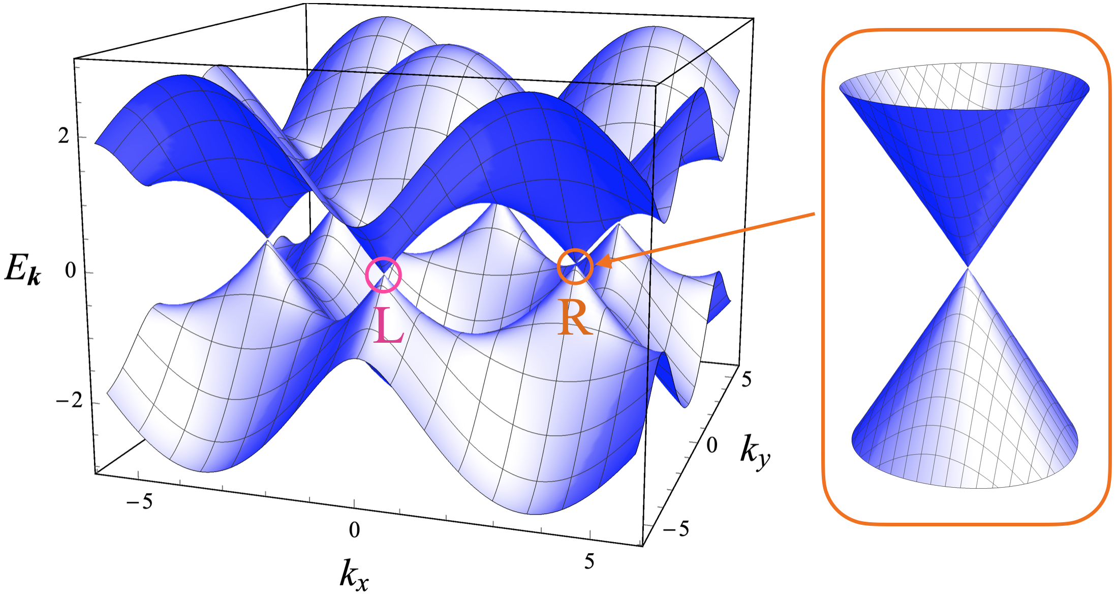
  Figure 1: Schematic dispersion relation of graphene. The Fermi level is located at the band crossings and the energy is bounded defining a compact Fermi sea.

  Massless Dirac fermions appear in condensed matter as the low energy effective description of electronic systems whose Fermi level sits near a two-band crossing. The Nielsen-Ninomiya theorem Nielsen and Ninomiya (1981) ensures that these crossings appear always in pairs of opposite chiralities. Real crystals typically host more than one pair of chiral fermions, usually close to high-symmetry points or planes. Restricting to a single pair, Dirac semi-metals are those three-dimensional crystals where the two chiralities sit at the same point in energy-momentum space (as massless Dirac particles). To realize a Weyl semimetal (isolated Weyl nodes) either inversion or time-reversal (or both) need to be absent, which allows the two chiralities to be separated in either energy or momentum (or both). A detailed description of these conditions and materials that realize them can be found in several recent reviews Jia et al. (2016); Yan and Felser (2017); Armitage et al. (2018).

  Fig. 1 shows the band structure of graphene, the material which made “Dirac fermions” popular in condensed matter. There are two inquivalent momenta, or ”valleys”, in the Brillouin zone where the dispersion is linear, marked as L, R in the figure. These are refered to as massless Dirac points. As mentioned in the introduction of this section, being a two dimensional material, the two valleys of graphene are not Weyl fermions. The dispersion relation shown is visually similar to the band structure of a (say, constant $k_{z}$) cut of a three dimensional Weyl semimetal. As seen in Fig. 1, the bands of the two valleys are connected in the Brillouin zone.

  In condensed matter realizations, in addition to the two band crossings described by the Dirac or Weyl equation (linear dispersion relation), the name of Dirac matter may be used to refer to other systems described by more exotic equations involving also Dirac matrices. Most noticeable are multi-Weyl fermions with different dispersion relations along different symmetry axis, higher-order polynomial dispersion relations, nodal Weyl semimetals which host a line of nodal points, and multifold fermions, which have point degeneracies of multiple bands Has (2021) modelled by higher-spin generalizations of Weyl fermions. The phenomena described in this review do not necessarily apply to these systems, defining in turn an interesting research frontier. In what follows, when we refer to Dirac matter we mean systems described by the QFT massless Dirac equation with linear dispersion relation.

• The vacuum

  The QFT vacuum refers to fields at zero temperature $T$ and chemical potential $\mu$. Originally, anomalies were formulated in vacuum and the role at finite temperature $T$ and chemical $\mu$ has only been fully appreciated recently. In condensed matter realizations, $T=0$ and $\mu=0$ are fined tuned, possibly unrealistic, limits. Most importantly, the QFT fermionic vacuum is the Dirac sea, an infinite tower of negative energy occupied levels. In contrast, the number of occupied electronic states below the Fermi surface (the condesned matter vacuum), is always finite (see Fig. 1). So in the QFT intuitive description of the chiral anomaly, left (right) particles are annihilated and created from the vacuum. Strong enough fields can also create pair of states from the vacuum as in the Schwinger mechanism Schwinger (1951). In the condensed matter realization, the two chiralities are connected through the bottom of the band (see Fig. 1) so the “spectral flow” of QFT Landsteiner (2016) reduces to a shift of particles in the same band.

• A note on Lorentz invariance

  The Dirac equation (4) assumes the invariance of the theory under the group of Lorentz transformations, which include boosts and spatial rotations as well as time-reversal and parity transformations. The Lorentz invariance reflects itself in the form of the kinetic term, $\gamma^{\mu}\partial_{\mu}\equiv\gamma^{0}\partial_{t}+c{\vec{\gamma}}\cdot{\vec{\nabla}}$, where $c$ is the speed of light. Since both the massless fermions and photons propagate with the same velocity $c$, the full interacting theory, which includes the kinetic terms for photons and particles, is invariant under Lorentz boosts.

  In Dirac and Weyl semimetals, however, the quasiparticle excitations propagate with the Fermi velocity $v_{F}$, which is much slower than the speed of light. The quasiparticles are described by the same Dirac equation (4) which is, however, modified by the substitution $c\to v_{F}$ in the derivative term: $\gamma^{\mu}\partial_{\mu}\to\gamma^{0}\partial_{t}+v_{F}{\vec{\gamma}}\cdot{\vec{\nabla}}$, where we assumed for a moment the isotropy and homogeneity of the spacetime as seen by the low-energy quasiparticles. Due to the inequivalence of the velocities of matter fields and interaction carriers, $v_{F}\neq c$, the kinetic term of quasiparticles (2) loses the invariance under the Lorentz transformations.

  The Lorentz symmetry breaking in condensed matter enriches the physics of the Dirac quasiparticles without spoiling the self-consistency of the appropriate low-energy models. We refer to Refs. Armitage et al. (2018); Grushin (2019) for a more detailed discussion on this topic which is touched in our review only in bypassing.

• The Bloch theorem

  Intuitively a (transport) current moves ”something” from a place A in space to another place B. To make this statement a bit more meaningful we also demand that the ”something” is stable and does not decay in the timespan in which the transport process takes place. A current transports therefore (approximately) conserves charges. Energy and electric charge are exactly conserved, spin or axial charge might be only approximately conserved. If the physical system under consideration is in its lowest energy state, e. g. is in thermodynamic equilibrium, one would not expect such motion to be possible, since this would be a realization of a form of a perpetuum mobile. This intuition is formalized in a theorem stated by Felix Bloch in the 1930s which was later summarized by D. Bohm in Ref. Bohm (1949). Originally it states that it is not possible for a condensed matter system residing in a thermodynamic limit to support an electric current in equilibrium Bohm (1949). A more modern formulation states that the net current corresponding to an exactly conserved $U(1)$ charge has to vanish in thermodynamic equilibrium. A quick argument goes as follows. The coupling of the current in the Hamiltonian is

  $$H_{\mathrm{int}}=\int d^{3}r\vec{A}\cdot\vec{J}\,.$$ (8)

  For an exactly conserved $U(1)$ charge the field $\vec{A}$ is a gauge field. This means that a spatially constant and time independent value of the gauge potential $\vec{A}$ should have no physical consequence. If the current has however an expectation value $\langle{\vec{J}}\rangle\neq 0$ then an infinitesimally small variation of the gauge potential $\delta{\vec{A}}$ results in the energy change

  $$\langle\delta H_{\mathrm{int}}\rangle=\delta{\vec{A}}\cdot\int d^{3}x\langle\vec{J}\rangle,$$ (9)

  which can be negative and thus would allow to lower the energy of the system. This contradicts the assumption that the system is in the lowest energy state. It follows that for an exactly conserved $U(1)$ current

  $$\int d^{3}r\,\vec{J}(\vec{r})=0\,.$$ (10)

  We note that this condition does not rule out circular (persistent) magnetization currents nor does it rule out superconducting currents. In the former case the system resides in a finite (topologically equivalent to a ring) volume far from the thermodynamic limit. The geometry of the system imposes a quantization constraint on the gauge field ${\vec{A}}$ via the Aharonov-Bohm phase which does not allow for infinitesimally small variations of the gauge potential $\delta{\vec{A}}$. Therefore, the Bloch no-current theorem does not work for persistent currents. In a superconductor, the gauge symmetry is spontaneously broken and a state with a non-vanishing supercurrent can only be a metastable state.

  On the other hand if the current is not exactly conserved or is affected by an anomaly the vector $\vec{A}$ is strictly speaking not a gauge field but a physical observable by itself. Therefore the system with $\vec{A}\neq 0$ is not equivalent to the ground state in the system $\vec{A}=0$ but rather a different physical system with a new Hamiltonian. Therefore the Bloch theorem does not apply in this situation and equilibrium currents are possible for this type of currents. A recent quantum field theory discussion of the Bloch theorem can be found in Yamamoto (2015), and a modern formulation for lattice Hamiltonians is in Watanabe (2019). A generalization of the Bloch theorem to the energy current of Hamiltonian lattice systems has been given in Kapustin and Spodyneiko (2019).

III Thermal and electro-thermal transport

Thermal transport refers generically to transport of energy, charge, or any other property under the effect of a gradient of temperature. In metals most transport phenomena are dominated by the free electrons that conduct energy, and charge. In principle phonons can also contribute to the thermal conductivity. Since we are mainly interested in the thermal transport properties of fermions (electrons) described by the Dirac equation we will not consider the phonon contribution. For standard metals describable as Fermi liquids, the thermal conductivity is proportional to the electric conductivity (Wiedemann-Franz law). Generically this can be seen as a sign of the existence of long lived quasi-particles. When these quasi particles obey a Dirac or Weyl equation they are subject to the effects of anomalies. As we will see in section V the Wiedemann-Franz law holds for the anomaly induced conductivities in the presence of a magnetic field (magneto–thermal transport).

We start from the phenomenological equations describing electric and energy transport as a response to electric fields and gradients of chemical potential and temperature Luttinger (1964)

$${\vec{J}}_{\textrm{tr}}=\bm{L}^{(1)}\left({\vec{E}}-T{\vec{\nabla}}\frac{\mu}{T}\right)+\bm{L}^{(2)}T{\vec{\nabla}}\frac{1}{T},$$ (11)

$${\vec{J}}_{\textrm{tr}}^{\,\mathcal{E}}=\bm{L}^{(3)}\left({\vec{E}}-T{\vec{\nabla}}\frac{\mu}{T}\right)+\bm{L}^{(4)}T{\vec{\nabla}}\frac{1}{T}.$$ (12)

The currents $\vec{J}_{tr}$ and $\vec{J}^{\mathcal{E}}_{tr}$ are the particle current and energy current respectively, with the particle current related to the electrical current as $\vec{J}^{e}_{tr}=-e\vec{J}_{tr}$ ($-e$ is the electron charge). The tensors $\bm{L}^{(i)}$ are the transport coefficients, and $\vec{E}$ is the electric field. The Onsager relations Onsager (1931) relate the second and third transport coefficients as $\bm{L}^{(2)}=\bm{L}^{(3)}$, or $L^{(2)}_{ij}(B)=L^{(3)}_{ji}(-B)$ in the presence of a magnetic field (see Sec. IV). The first terms inside the parenthesis in Eqs. (11) and (12) represent the Einstein relation Sutherland (1905); Einstein (1905); von Smoluchowski (1906); Luttinger (1964), which states that in equilibrium an electric field is compensated by an opposing gradient of chemical potential and temperature $\vec{E}=T\vec{\nabla}(\mu/T)$. The energy current ${\vec{J}}_{\textrm{tr}}^{\,\mathcal{E}}$ results from the combination of heat current $\vec{J}^{Q}$ and energy transported by the particle current ${\vec{J}}_{\textrm{tr}}$; the heat current can therefore be written as

$${\vec{J}}_{\textrm{tr}}^{\,Q}={\vec{J}}_{\textrm{tr}}^{\,\mathcal{E}}-\mu{\vec{J}}_{\textrm{tr}}.$$ (13)

The currents in Eqs. (11) and (12) are transport currents which means they represent net transport through a cross section of the given material. As such, they should vanish in equilibrium. It is important to carefully distinguish between the transport currents $\vec{J}_{\textrm{tr}}$ relevant to Eqs. (11) and (12), and the total local currents $\vec{J}$ at any given point in the sample Smrcka and Streda (1977); Cooper et al. (1997); Bradlyn and Read (2015). While in time-reversal invariant systems these coincide, breaking time-reversal symmetry can lead to the appearance of magnetization electric and energy currents. These are defined as divergenceless circulating currents which average to zero and therefore do not carry any transport Cooper et al. (1997). We will discuss the presence of magnetization currents in more detail in Sec. IV.

Let us now fix the chemical potential and allow for gradients of temperature, and consider a sample disconnected from current leads such that no net electric current flows. In this situation, the transport electric current vanishes and an electric field is generated. From the transport Eqs. (11) and (12), and using Eq. (13) we have

$${\vec{E}}={\bf S}{\vec{\nabla}}T,$$ (14)

$${\vec{J}}^{Q}_{\textrm{tr}}=-{\bf K}{\vec{\nabla}}T,$$ (15)

where the thermopower $\bm{S}$ (or Seebeck coefficient) and thermal conductivity $\bm{K}$ tensors are functions of the transport coefficients:

$$\bm{S}=\frac{1}{T}\big{[}\bm{\rho}\bm{L}^{(2)}-\mu\big{]},$$ (16)

$$\bm{K}=\frac{1}{T}\big{[}\bm{L}^{(4)}-\bm{L}^{(3)}\bm{\rho}\bm{L}^{(2)}\big{]}.$$ (17)

where $\rho$ is the resistivity tensor $\bm{\rho}=\bm{\sigma}^{-1}$, and we have renamed $\bm{L}^{(1)}\equiv\bm{\sigma}$, which is the most established notation for the electric conductivity.

Eq. (14) gives rise to the Seebeck effect, which is an expression of the longitudinal components of (11): generation of an electric potential in the direction of a temperature gradient.

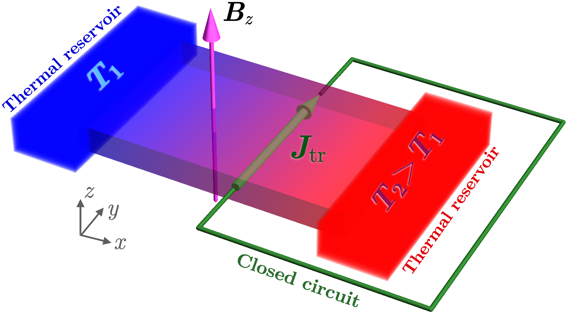
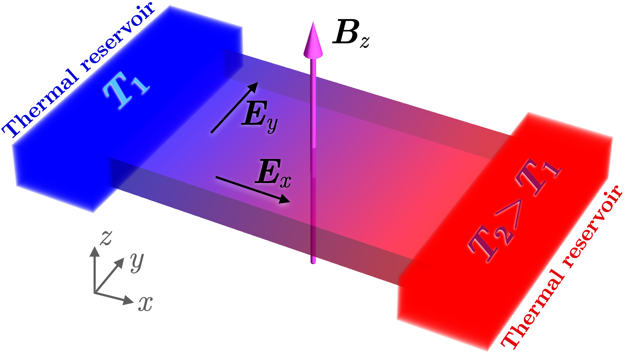
(a)	(b)

Figure 2: A system consisting of a sample (a) connected to and (b) disconnected from current leads, in an external magnetic field, attached to two thermal reservoirs at different temperatures such that a thermal gradient is generated through the sample. (a) A transport current flows in the direction perpendicular to both the magnetic field and gradient of temperature, corresponding to the Nernst current, Eq. (18); (b) An electric current cannot flow, so the electric fields $E_{x}$ and $E_{y}$ are generated in the plane perpendicular to the magnetic field direction, corresponding to the Nernst-Ettingshausen (20) and Nernst (19) coefficients respectively.

The Nernst-Ettingshausen effects occur in the presence of a magnetic field. The Nernst effect refers to the generation of an electric current perpendicular to a temperature gradient and to the applied magnetic field, Fig. 2(a):

$$\vec{J}\propto\vec{B}\times\vec{\nabla}T.$$ (18)

For a sample disconnected from current leads, a compensating electric field must necessarily appear such that the transport current vanishes. This situation is schematically described in Fig. 2. If we choose the gradient of temperature to point, say, along the $\hat{x}$ direction, $\nabla_{x}T$, and the magnetic field $\vec{B}$ to point along $\hat{z}$, two coefficients are usually defined: the Nernst coefficient

$${\cal N}_{yx}\equiv\frac{E_{y}}{B_{z}\partial_{x}T}=\frac{\rho_{yi}L^{(2)}_{ix}}{B_{z}}.$$ (19)

and the Ettingshausen-Nernst coefficient:

$${\cal N}_{xx}\equiv\frac{E_{x}}{B_{z}\partial_{x}T}=\frac{\rho_{xi}L^{(2)}_{ix}-\mu}{B_{z}},$$ (20)

see Fig. 2(b).

III.1 Thermoelectric relations

In the standard model for metals, the Fermi liquid, the thermo–electric coefficients in Eqs. (11),(12) obey certain phenomenological relations, the main ones being the Wiedemann-Franz law and the Mott relation Ziman (1960); Jonson and Mahan (1980):

$$\bm{K}=LT\bm{\sigma}(T=0),$$ (21)

$$\bm{S}=LT\bm{\rho}(T=0)\frac{d\bm{\sigma}(T=0)}{d\mu}{\biggl{|}}_{\mu=\epsilon_{F}/e}.$$ (22)

The Wiedemann-Franz law (21) establishes that the ratio of the thermal to the electrical conductivity is the temperature times a universal number, the Lorenz number $L=\pi^{2}k_{B}^{2}/3e^{2}$, where $k_{B}$ is the Boltzmann constant. The Mott relation (22) relates the thermopower with the derivative of the electrical conductivity with respect to the chemical potential at the Fermi level. Note that the electric conductivity in Eqs. (21) and (22) is evaluated at zero temperature, as both the Mott rule and the Wiedemann-Franz law are obtained as an expansion in $k_{B}T\ll|\mu|$. The Mott and Wiedemann-Franz relations hold for transport currents only Smrcka and Streda (1977); Jonson and Girvin (1984); Cooper et al. (1997); Qin et al. (2011), which means that in systems that break time-reversal symmetry the local currents do not generally fulfill them (see Sec. IV). The validity of these laws has been established for any system which can be described as a Fermi liquid, provided the quasiparticles do not exchange energy during collisions. The validity has also been proven to be valid when a semi-classical description (as the Boltzmann formalism) of the electronic system is justified. Deviations from these phenomenological relations in conventional matter are normally attributed to electron–electron interactions inducing departures from Fermi liquid behavior or to the emergence of a new phase regime. In particular the relations might not apply when the systems are in the hydrodynamic regime.

Topological materials have anomalous conductivities (particularly the Hall conductivity) similar to that occurring in ferromagnetic materials, induced by the Berry curvature of the bands. The question of whether or not these anomalous transport coefficients obeyed the Wiedemann-Franz and Mott relations, arose soon after the recognition of the topological properties. Berry curvature effects were included in the Boltzmann transport formalism in a way to fulfil the rules Xiao et al. (2006); Ryu et al. (2012), but the experimental situation is more uncertain and violations of the thermoelectric relations have been reported in some materials Pu et al. (2008); Kim (2014); Liang et al. (2014); Li et al. (2015).

Typically Dirac materials in two and three dimensions are expected to follow the standard relations in the low $T$ regime and deviate from it at larger temperatures Liang et al. (2017); Gorbar et al. (2017a); Jaoui et al. (2018). Violations of the Wiedemann-Franz law have been described in these systems associated to the presence of a hydrodynamic regime where departures from the standard Fermi liquid behavior are also found Lucas et al. (2016); Gooth et al. (2018). In sec. 4 we will see that the anomaly-related transport coefficients fulfil these relations although a different claim has been made recently in Ref. Das and Agarwal (2020a).

III.2 Luttinger theory of thermal transport coefficients

Transport coefficients are computed in the framework of linear response theory: the currents are obtained as a response to an applied field, usually by the derivation of the corresponding Kubo formulas. The electrical current results from the response to an applied electric field, which, if the given system is in equilibrium, is compensated by a gradient of chemical potential: $\vec{E}=\vec{\nabla}\mu$. This relation, the Einstein relation, is what sets the link between linear response to a field (electric field) and the response to a statistical force (the gradient of the chemical potential) (see Eq. (11)). It permits to compute the response to a statistical force through linear response theory.

A question therefore naturally arises in the context of thermal transport: what is the “thermal field” needed to develop a linear response theory of thermal transport? What is the equilibrium relation for the other statistical force, the gradient of temperature? In 1964, Luttinger solved these problems by showing that the gravitational field can play the role of the “thermal field” Luttinger (1964). By coupling the gravitational field to the electronic degrees of freedom he developed the linear response theory for thermal transport. In this section we review and contextualize Luttinger’s theory and ideas.

III.2.1 Tolman–Ehrenfest pioneering work: Thermodynamic equilibrium in gravitational fields

The earliest link that opened the door to relate gravitational effects with thermal transport in condensed matter systems was set up by the works of Tolman and Ehrenfest in 1930 Tolman (1930); Tolman and Ehrenfest (1930) when trying to adapt the thermodynamic relations to general relativity. The underlying idea that “heat has weight” let them to conclude that, in a gravitational field, thermal equilibrium must be accompanied by a temperature gradient in order to prevent the flow of heat from regions of higher to those of lower gravitational potential. The basic equation defining equilibrium in a curved background was set to be

$$T\sqrt{g_{tt}({\vec{r}})}={\rm constant}.$$ (23)

In a weak gravitational field $\phi$,

$$g_{tt}({\vec{r}})=1+2\phi({\vec{r}})/c^{2},$$ (24)

where we restore $c$ as the speed of light, we get the relation

$$\frac{1}{T}{\vec{\nabla}}T=-\frac{1}{c^{2}}{\vec{\nabla}}\phi\,.$$ (25)

This relation was first obtained by Tolman Tolman (1930) for a spherical mass distribution and it was later generalized by Tolman and Ehrenfest Tolman and Ehrenfest (1930) to general -static- gravitational fields. As a consequence, the temperature variation in a gravitational field inducing the acceleration $g$ was

$$\frac{1}{T}\frac{dT}{dr}=-\frac{g}{c^{2}}.$$ (26)

The estimate of the temperature variation at the surface of the earth given by Tolman in Ref. Tolman (1930) was

$$\frac{1}{T}\frac{dT}{dr}=-\frac{g}{c^{2}}\sim-10^{-18}{\mathrm{cm}}^{-1}.$$ (27)

Despite the small magnitude of the effect, the underlying ideas provided the basis for the Luttinger theory of thermal transport widely used in condensed matter Luttinger (1964).

The relation (25) defining thermodynamic equilibrium in gravitational fields with specific distributions of matter, was later extended to the presence of a finite chemical potential Klein (1949). This issue have been revised in recent works Santiago and Visser (2018, 2019); Lima et al. (2019). We will see a formal derivation in Sec. III.4.

III.3 Kubo formulas for the thermal and thermoelectric conductivities

The previous ideas were used by Luttinger to derive a Kubo formula for the thermal transport coefficient Luttinger (1964). In linear response theory Giuliani and Vignale (2005), the transport coefficients can be written in terms of the retarded current-current two-points function. A common example is the expression of the electrical conductivity Kubo (1957):

$$J^{i}=\sigma^{ij}E_{j}\quad,\quad E_{j}=i\omega A_{j};$$ (28)

$$\sigma^{ij}(\omega)=\frac{1}{i\omega}\langle J^{i}J^{j}\rangle(\omega,k=0).$$ (29)

The Kubo formula is based on the possibility of adding a local source ($A_{\mu}$) to the current ($J^{\mu}$) in the action in the standard way:

$$S[J]=S_{0}-\int d^{4}xJ^{\mu}A_{\mu},$$ (30)

so that

$$J^{\mu}=-\frac{\delta S}{\delta A_{\mu}}.$$ (31)

The difficulty to apply this approach to thermal transport lies in finding the appropriate local source coupling to heat (or energy) density. Early attempts were made by considering macroscopic thermodynamic variables as local variables by dividing the system in small portions and making some assumptions about how these variables develop in time Green (1952); Kubo et al. (1957); Mori (1958).

Luttinger Luttinger (1964) aimed to give a mechanistic sustain to what he called Green-Kubo-Mori formulas. Proceeding by analogy with the electrical conductivity, he proposed the introduction of a (fictitious) inhomogeneous gravitational field $\phi(r)$ which causes energy or heat currents to flow as a response to gradients of $\phi(r)$. This formalism is clear in special relativity, where the energy momentum tensor of a generic matter field $\phi$ is the conserved current associated to metric variations due to Lorentz invariance:

$$T^{\mu\nu}(\Phi)=-\frac{2}{\sqrt{-g}}\frac{\delta S[\Psi,g]}{\delta g_{\mu\nu}},$$ (32)

where $\Psi$ represents matter fields. In particular, the energy current is given by the components $J_{\mathcal{E}}^{i}=T^{0i}$. For small deviations from flat space the gravitational potential $\phi$ is proportional to the zero-zero component of the metric: $g^{00}=1+2\phi$, which couples to the energy density $T^{00}$. Here we follow Luttinger (1964) and absorbed the velocity $c$ into the gravitational potential $\phi\rightarrow c^{2}\phi$. This rescaled gravitational potential is simply the field that couples to the energy density. The perturbed Hamiltonian to be used in the linear response formalism is Luttinger (1964)

$$H_{\mathrm{int}}(t)=\int d^{3}r\;h({\vec{r}},t)\phi(t,\vec{r}),$$ (33)

where $h({\bf r},t)$ is the Hamiltonian density. We can write the coefficients for the local current densities as responses to the external fields $A_{0}$ and $\phi$

$$\vec{J}={\bm{\mathcal{L}}}^{(1)}\vec{E}-{\bm{\mathcal{L}}}^{(2)}\vec{\nabla}\phi,$$ (34)

$$\vec{J}^{\mathcal{E}}={\bm{\mathcal{L}}}^{(3)}\vec{E}-{\bm{\mathcal{L}}}^{(4)}\vec{\nabla}\phi,$$ (35)

which can in turn be written in terms of correlations of the currents. Note we use ${\bm{\mathcal{L}}}^{(i)}$ in Eqs. (34), (35) to denote the coefficients that determine the local currents obtained from Kubo formulas, and $\bm{L}^{(i)}$ in Eqs. (11), (12) to denote the coefficients that determine transport currents. The tensors ${\bm{\mathcal{L}}}^{(i)}$ and $\bm{L}^{(i)}$ may differ if magnetization currents are present, which are discussed in section IV.2. The thermal and thermoelectric coefficients ${\bm{\mathcal{L}}}^{(2)}$ and ${\bm{\mathcal{L}}}^{(4)}$ can be computed as Luttinger (1964)

$${\mathcal{L}}^{(2)}_{ij}=\lim_{\omega\to 0}\frac{1}{i\omega}\langle J^{\mathcal{E}}_{i}J_{j}\rangle(\omega,k=0),$$ (36)

$${\mathcal{L}}^{(4)}_{ij}=\lim_{\omega\to 0}\frac{1}{i\omega}\langle J^{\mathcal{E}}_{i}J^{\mathcal{E}}_{j}\rangle(\omega,k=0).$$ (37)

The use of the gravitational field coupling to the energy density whose variations induce energy currents is the first main contribution of Luttinger’s work. Still the issue remains as how to couple the statistical force (temperature gradient) to the energy current. The passage from Eqs. (34), (35) to Eqs. (11), (12), (this is, the relation between ${\bm{\mathcal{L}}}^{(i)}$ and $\bm{L}^{(i)}$) was first presented in the original work by Luttinger Luttinger (1964). In what follows we will show a different re–formulation of the Luttinger approach more suitable for making the connection with other aspects of the review.

III.4 Formal derivation of generalized Luttinger relations

Here we present a formal approach to generalized Luttinger relations. It is based on introducing external fields to mimic variations in thermodynamic parameters, the temperature $T$, chemical potential $\mu$ and velocities $u_{a}$ (see Appendix A). This allows to derive Kubo formulas for electric and thermal conductivities from a unifying principle or, more generally, for transport coefficients appearing in an effective hydrodynamic description of a physical system.

We start from the very basic assumption that we have an action given as a functional of the metric and a gauge field

$$S=S[g,A]\,.$$ (38)

The precise form of this function will depend on the underlying physical theory but we are only interested in the way a system described by $S$ reacts to changes in the external fields, the metric and the gauge field. We can define the energy-momentum tensor through variations of the metric (see Eq. (32)) and the electric current through variations of the gauge field:

$$J^{\mu} =-\frac{1}{\sqrt{-g}}\frac{\delta S}{\delta A_{\mu}(x)}\,.$$ (39)

If the action is invariant under diffeomorphisms and gauge transformations the current and energy-momentum tensor (32) obey conservation laws. The conserved momentum and charge can be obtained by integrating over the spatial volume

$$P_{\mu} =\int d\Sigma\,T^{t}_{\mu}\,,$$ (40)

$$Q =\int d\Sigma\,J^{t}\,.$$ (41)

The time component of the four-vector $P_{\mu}$ is the total energy (the Hamiltonian) and the spatial components are the (spatial) momenta. Now we can form the general statistical operator (see Appendix A)

$$\rho=\exp\left[-\frac{1}{T}\left(u^{\nu}P_{\nu}-\mu Q\right)\right]\,,$$ (42)

where $u^{\nu}$ is a four velocity, $T$ the temperature and $\mu$ the chemical potential. We will assume an ensemble at rest with $u^{\nu}=(1,0,0,0)$. The four-velocity is constrained to be a time-like unit vector $u^{2}=1$. This constraint is solved by writing

$$u^{\mu}=\left(\frac{1}{\sqrt{1-\vec{\beta}^{2}}},\frac{\vec{\beta}}{\sqrt{1-\vec{\beta}^{2}}}\right)\,,$$ (43)

in terms of a purely spatial velocity $\vec{\beta}=\vec{v}/c$. Here $c$ can be interpreted as the speed of light in the context of high-energy physics or as the Fermi-velocity in a Dirac material.

We are interested on the effect that a variation of the gauge field and metric has on the thermal ensemble. For simplicity and because it is also the most relevant case in condensed matter applications we consider the case of a small metric perturbation on top of a flat background geometry $g^{\mu\nu}=\mathrm{diag(1+\delta g^{tt},-1,-1,-1)}$. By the definitions (32) and (39), we can find the change of the Hamiltonian under small and constant variations of the temporal component $A_{t}$ of the gauge field and the $g^{tt}$ component of the metric. Since in terms of the kinetic ($T$) and the potential ($V$) the action and the Hamiltonian can be written as $S=T-V$ and $H=T+V$, respectively, it follows that $\delta S=-\delta H$ if the variation $\delta$ only concerns $V$, as it does here. From this it follows that

$$\delta H=-\frac{1}{2}\delta g^{tt}H+\delta A_{t}Q\,,$$ (44)

So far we have changed the microscopic Hamiltonian by switching on small increments in gravitational and electrostatic potential. Now we want to ask if we can mimic the effects of these increments by introducing small variations in the thermodynamic variables $T$ and $\mu$. In other words we now keep the microscopic Hamiltonian fixed but change that state thermodynamic state characterised by increments $T+\delta T$ and $\mu+\delta\mu$. We demand therefore that the statistical operators of the new system with $\delta g^{tt}$ and $\delta A_{t}$ are equivalent to the statistical operator of the old system in the new state $T+\delta T$ and $\mu+\delta\mu$

$$\exp\left[-\frac{1}{T}(H+\delta H-\mu Q)\right]=\exp\left\{-\frac{1}{T}\left[\left(1-\frac{1}{2}\delta g^{tt}\right)H-(\mu-\delta A_{t})Q\right]\right\}=\exp\left[-\frac{1}{T+\delta T}(H-(\mu+\delta\mu)Q)\right].$$ (45)

To first order in $\delta T$ and $\delta\mu$ and introducing the Newtonian potential $\phi=-\delta g^{tt}/2$ this leads to the conditions

$$\phi =-\frac{\delta T}{T}=T\delta\left(\frac{1}{T}\right)\,,$$ (46)

$$\delta A_{t} =-\delta\mu+\mu\frac{\delta T}{T}=-T\delta\left(\frac{\mu}{T}\right)\,.$$ (47)

Finally, we can also study the consequences of the variation $\delta g^{xt}$. It leads to

$$\delta H=-\delta g^{xt}P_{x}\,,$$ (48)

which leads to a shift in the fluid velocity

$$\delta u^{x}=-\delta g^{xt}\,.$$ (49)

In this way variations in the external fields can be translated into variations in the thermodynamic variables. While these considerations apply to equilibrium and for spatially uniform variations they also apply in the presence of spatial gradients if we assume that the system is in local thermal equilibrium. The assumption of local thermal equilibrium implies that gradients are small on length scales of the order of the mean free path and that thermodynamic relations hold locally. More precisely a system in local thermal equlibrium can be described by local and time dependent temperature $T(t,\vec{x})$, chemical potential $\mu(t,\vec{x})$ and fluid velocity $u^{\mu}(t,\vec{x})$. Under these conditions it is legitimate to substitute $\delta\rightarrow\vec{\nabla}$ in (46), (47) and (49). These relations imply that the condition for remaining in equilibrium are

$$-\vec{\nabla}A_{t}-T\vec{\nabla}\left(\frac{\mu}{T}\right)= 0\,,$$ (50)

$$\vec{\nabla}\phi-T\vec{\nabla}\left(\frac{1}{T}\right)= 0$$ (51)

These equations are however neither gauge invariant nor relativistically covariant. Whereas it is clear that gauge invariance implies the substitution $-\vec{\nabla}A_{t}\rightarrow\vec{E}$, it is not immediately clear how a covariant term for the gravitational potential can be written. The problem is that there is no covariant tensor that can be constructed out of the metric and its first derivatives. Indeed the curvature tensor $R_{\alpha\beta\mu\nu}$ is second order in derivatives on the metric. It is possible however to write down a term of the correct form with the help of the velocity field $u^{\mu}$. An appropriate phenomenological constitutive relation that is first order in derivatives, gauge invariant and covariant is

$$J^{\mu}=\rho u^{\mu}+P_{\perp}^{\mu\nu}\left[\sigma\left(E_{\nu}-T\nabla_{\nu}(\frac{\mu}{T})\right)+\kappa T\nabla_{\nu}(\frac{1}{T})+\xi u^{\lambda}\nabla_{\lambda}u_{\nu}\ \right]\,.$$ (52)

Here $\rho$ is the charge density (or energy density if we consider the energy current) and $P_{\perp}^{\mu\nu}=g^{\mu\nu}-u^{\mu}u^{\nu}$ is the projector transverse to $u^{\mu}$. This ensures the $u_{\mu}J^{\mu}=\rho$ without any first order term in derivatives. The covariant electric field is $E_{\mu}=F_{\mu\nu}u^{\nu}$. The last term depends on the frame vector $u^{\mu}$ only. Expanding around a flat metric $g_{\mu\nu}=\eta_{\mu\nu}+\delta g_{\mu\nu}$ and in the rest frame $u^{\mu}=(1,0,0,0)$ this last term becomes

$$P^{\mu\nu}_{\perp}u^{\lambda}\nabla_{\lambda}u_{\nu}=-\delta^{\mu i}\nabla_{t}u_{i}=-\delta^{\mu i}(\delta\dot{g}_{it}-\frac{1}{2}\partial_{i}\delta g_{tt})=-\delta^{\mu i}E_{i}^{g}$$ (53)

where $E_{i}^{g}$ is the gravito-electric field (see Appendix D). It is therefore the covariant term that encodes the action of the gravitational field in analogous way of the electric field. The condition that in equilibirium the current should vanish implies then $\xi=-\kappa$. The physical interpretation of $u^{\lambda}\nabla_{\lambda}u_{\nu}$ is a covariant version of the acceleration.

We note that $h_{ti}$ can be viewed as a gravito-magnetic vector potential $A_{g,i}$. A vector field as source for the energy current will further be discussed in section IV.2.

Luttinger’s transport equations

We can, at this point, complement Eqs. (11), (12) by including Luttinger’s gravitational potential. From the relation (51) we can write

$$\vec{J}_{\textrm{tr}}=\bm{L}^{(1)}\left(\vec{E}-T\vec{\nabla}\frac{\mu}{T}\right)+\bm{L}^{(2)}\left(-\vec{\nabla}\phi+T\vec{\nabla}\frac{1}{T}\right),$$ (54)

$$\vec{J}_{\textrm{tr}}^{\mathcal{E}}=\bm{L}^{(3)}\left(\vec{E}-T\vec{\nabla}\frac{\mu}{T}\right)+\bm{L}^{(4)}\left(-\vec{\nabla}\phi+T\vec{\nabla}\frac{1}{T}\right).$$ (55)

From Eqs. (50) and (51) we see that, in equilibrium, $\vec{J}_{tr}=\vec{J}^{\epsilon}_{tr}=0$. This is correct, since $\vec{J}_{tr}$, $\vec{J}^{\epsilon}_{tr}$ are transport currents and should vanish in equilibrium. It is clear now what is the relation between the coefficients computed by the Kubo-formulas (${\bm{\mathcal{L}}}^{(i)}$), Eqs. (34) and (35), and the transport coefficients:

$${\bm{\mathcal{L}}}^{(i)}=\bm{L}^{(i)}\,,\qquad\mbox{(no magnetisation current)}\,,$$ (56)

There is still a small, or perhaps not that small, caveat here. The relation ${\bm{\mathcal{L}}}^{(i)}=\bm{L}^{(i)}$ only generally holds in time-reversal invariant systems, where magnetization currents are absent. The Kubo-formula coefficients capture the total local current at any given point in the sample. This includes contributions from magnetization currents. But because magnetization currents do not contribute to transport, ${\bm{\mathcal{L}}}^{(i)}=\bm{L}^{(i)}$ no longer holds. We will discuss this further in section IV.

IV Transport and magnetization currents

IV.1 General remarks

In systems where time-reversal symmetry is broken, the definition of transport currents, measured in transport experiments becomes more subtle due to the presence of magnetization currents. Magnetization currents are circulating currents that arise when time-reversal symmetry is broken. These appear for instance in the presence of an external magnetic field, and do not contribute to the net transport through the sample. Therefore, in general, the local particle and energy currents $\vec{J}$, $\vec{J}^{\epsilon}$, as given by the Kubo formulas, are written as the sum of transport plus magnetization currents

$$\vec{J}=\vec{J}_{\mathrm{tr}}+\vec{J}_{\mathrm{mag}},\quad\vec{J}^{\epsilon}=\vec{J}^{\epsilon}_{\mathrm{tr}}+\vec{J}^{\epsilon}_{\mathrm{mag}}.$$ (57)

The magnetization currents can be defined as the rotational of a (energy) magnetization density

$$J_{i,\mathrm{mag}}=\epsilon_{ijk}\partial_{j}M_{k},\quad J^{\epsilon}_{i,\mathrm{mag}}=\epsilon_{ijk}\partial_{j}M^{\epsilon}_{k},$$ (58)

The magnetization vanishes outside the sample, and therefore $J_{i,\mathrm{mag}}$, $J^{\epsilon}_{i,\mathrm{mag}}$ average to zero over a cross-section of the sample. At vanishing external fields $A_{\mu}=\phi=0$, we can define the unperturbed magnetization densities $M_{0}^{i}(\mu,T)=M^{i}(A_{\mu}=\phi=0)$, $M_{0}^{\epsilon,i}(\mu,T)=M^{\epsilon,i}(A_{\mu}=\phi=0)$. In this situation, the magnetization is constant in the bulk, but because it vanishes outside the material, it will have a pronounced variation at the boundary giving rise to boundary magnetization currents. For non-vanishing external fields, $A_{t},\phi\neq 0$, the total magnetization density can be written in terms of the unperturbed magnetization Cooper et al. (1997):

$$\vec{M}=(1+\phi)\vec{M}_{0}(\mu,T),\quad\vec{M}^{\epsilon}=(1+2\phi)\vec{M}_{0}^{\epsilon}(\mu,T)+A_{t}\vec{M}_{0}(\mu,T),$$ (59)

and the bulk magnetization currents are then given by Cooper et al. (1997)

$$J_{i,\mathrm{mag}}=-\epsilon_{ijk}\left(M_{0,j}\partial_{k}\phi+\frac{\partial M_{0,j}}{\partial\mu}\partial_{k}\mu+\frac{\partial M_{0,j}}{\partial T}\partial_{k}T\right),$$ (60)

$$J^{\epsilon}_{i,\mathrm{mag}}=-\epsilon_{ijk}\left(-M_{0,j}E_{k}+2M^{\epsilon}_{0,j}\partial_{k}\phi+\frac{\partial M_{0,j}^{\epsilon}}{\partial\mu}\partial_{k}\mu+\frac{\partial M_{0,j}^{\epsilon}}{\partial T}\partial_{k}T\right).$$ (61)

To obtain the transport coefficients $\bm{L}^{(i)}$ defined in Eqs. (11) and (12), one should subtract the magnetization currents (for $\vec{\nabla}\mu=\vec{\nabla}T=0$) from the local currents (34), (35). The transport coefficients are then given in terms of the coefficients obtained from the Kubo-formulas, ${\bm{\mathcal{L}}}^{(i)}$, and the unperturbed magnetization densities

$$\bm{L}^{(1)} = {\bm{\mathcal{L}}}^{(1)}=\bm{\sigma},\hskip 42.67912ptL^{(2)}_{ij}={{\mathcal{L}}}^{(2)}_{ij}+\epsilon_{ijk}M_{0,k},$$ (62)

$$L^{(3)}_{ij} = {{\mathcal{L}}}^{(3)}_{ij}+\epsilon_{ijk}M_{0,k},\qquad L_{ij}^{(4)}={{\mathcal{L}}}_{ij}^{(4)}+2\epsilon_{ijk}M^{\epsilon}_{0,k},$$ (63)

The transport coefficients are related under time-reversal by Onsager relations Onsager (1931) as: $\sigma_{ij}(B)=\sigma_{ji}(-B)$, $L^{(4)}_{ij}(B)=L^{(4)}_{ji}(-B)$, $L^{(2)}_{ij}(B)=L^{(3)}_{ji}(-B)$, where $B$ denotes the magnetic field or any other parameter that breaks the time-reversal symmetry. It is important to state that it is the transport coefficients $\bm{L}^{(i)}$, and not the ones in the local currents, ${\bm{\mathcal{L}}}^{(i)}$, which fulfill the Mott rule and the Wiedemann-Franz law Smrcka and Streda (1977); Jonson and Girvin (1984); Cooper et al. (1997); Qin et al. (2011).

Transport currents are then obtained as a response to gradients of the statistical fields ($\mu$, $T$) by combining Eqs. (62), (63) and (54), (55), and setting $\vec{E}=\vec{\nabla}\phi=0$. To obtain the local currents as a response to $\vec{\nabla}\mu$, $\vec{\nabla}T$, the magnetization currents (60), (61) have to be added to the transport currents. This will give the total current locally at any point in the sample.

IV.2 Luttinger, thermal transport and energy magnetization

In section III.4 we introduced the Luttinger relation Eq. (25) as a gradient of a gravitational potential, and showed that we can include a thermal vector potential, in analogy with an electromagnetic field. The inclusion of a thermal vector potential turns out to be related to several issues and necessary extensions that concern the original work by Luttinger to capture a broader set of phenomena. First, unphysical divergences at $T\to 0$ have been encountered using the Luttinger derivation of the Kubo formula for thermal transport currents Qin et al. (2011); Tatara (2015). Second, Luttinger did not incorporate magnetization currents, which were added later Cooper et al. (1997); Smrcka and Streda (1977); Qin et al. (2011), resulting in (60) and (61). Lastly, the difference between diamagnetic and paramagnetic currents, explained below, is not as evident in the Luttinger formalism as they are in electromagnetism Tatara (2015).

The first two issues were addressed Cooper et al. (1997); Smrcka and Streda (1977); Qin et al. (2011) by noticing that the subtraction of the equilibrium magnetization currents from the result of linear response theory leads to well defined transport currents, see Eqs. (62), (63), even as temperature approached zero Qin et al. (2011). Tatara observed Tatara (2015) that a proper treatment of the diamagnetic heat current term will lead to this conclusion as well. In electromagnetism, the paramagnetic terms arise from terms in the Hamiltonian proportional to the vector potential $\vec{A}$, while diamagnetic terms stem from terms proportional to the square of $\vec{A}$. While the Dirac Hamiltonian only gives rise to paramagnetic terms because it is linear in momentum, the quadratic Schrödinger Hamiltonian will generically contain both paramagnetic and diamagnetic terms. In electromagnetism both terms are important as the paramagnetic current contains an equilibrium contribution determined by the electrons below the Fermi level which exactly cancels the diamagnetic current Tatara (2015). By formulating the Luttinger relation in terms of a vector potential, $\vec{A}_{g}$, Tatara was able to isolate the diamagnetic and paramagnetic contribution similarly to electromagnetism. This formulation reinterprets the results in Cooper et al. (1997); Smrcka and Streda (1977); Qin et al. (2011), sheds light into the issues and extensions discussed above related to the Luttinger approach, and emphasizes the parallelism between electromagnetism and gravitoelectromagnetism.

The emergence of a vector thermal potential $\vec{A}_{g}$ can be understood as arising from conservation laws Tatara (2015). In the Luttinger formalism the coupling to the gravitational field is imposed through the Hamiltonian density $h(\mathbf{r})$ given by $H_{\mathrm{int}}$ as written in (33)

$$H_{\mathrm{int}}=\int d^{3}{r}\;\phi(\vec{r})h(\vec{r}).$$ (64)

As discussed in Sec. III.4 the responses caused by a thermal gradient can be calculated in powers of $\nabla\phi$ and identifying $\vec{\nabla}\phi=-\frac{\vec{\nabla}T}{T}$ Luttinger (1964). Using the conservation law ${\partial}_{t}h(\vec{r})+\vec{\nabla}\vec{J}_{\epsilon}=0$, where $\vec{J}_{\epsilon}$ is an energy current, and restricting to steady-state properties, it is possible to rewrite this equation as

$$H_{A_{g}}=-\int d^{3}{r}\;\;\vec{J}_{\epsilon}(\vec{r},t)\cdot\vec{A}_{g}(\vec{r},t).$$ (65)

By identifying $\partial_{t}\vec{A}_{g}=-\frac{\vec{\nabla}T}{T}$, Tatara showed that the correct diamagnetic contribution is naturally captured, since $H_{A_{g}}$ depends explicitly on a vector potential. It is important to note that both formulations, either $H_{\mathrm{int}}$ or $H_{A_{g}}$ are equivalent. Both can incorporate magnetization currents and can be regular at $T\to 0$. The formalism in terms of $H_{A_{g}}$ allows to distinguish the diamagnetic contribution explicitly, and thus establishes a strong link between gravitoelectric fields and electromagnetic fields. Taking both $H_{\mathrm{int}}$ and $H_{A_{g}}$ together, a gauge degree of freedom emerges. So long as we are interested in steady-state properties, we are free to choose $\partial_{t}\vec{A}_{g}$ and $\vec{\nabla}\phi$ independently, so long as we identify $\vec{\nabla}\phi+\partial_{t}\vec{A}_{g}=-\frac{\vec{\nabla}T}{T}$ Tatara (2015).

The emergence of a vector thermal potential $\vec{A}_{g}$ has been described by resorting to the Newton-Cartan formalism Shitade (2014); Gromov and Abanov (2015); Bradlyn and Read (2015); Geracie et al. (2015). The conservation equations for momentum and energy densities follow from global space and time translations. To promote these to local symmetries one can define a local frame in terms of the vierbeins $e^{\mu}_{a}$. The resulting theory is similar to general relativity complemented by torsion, known as the Einstein-Cartan formalism described in sec. VIII and in Appendix B. If Lorentz symmetry is absent, as natural in condensed matter systems, it was suggested that the Newton-Cartan formalism is appropriate to describe the geometrical properties of the theory. Refs. Shitade (2014); Gromov and Abanov (2015); Bradlyn and Read (2015); Geracie et al. (2015) showed that by taking variations of the action with respect to $e^{\mu}_{a}$ and the metric, one can obtain the correct thermal transport and magnetization currents. In this formalism both $\vec{A}_{g}$ and $\phi$ appear naturally, as a consequence of local coordinate transformations.

It is important to point out that the results of Refs. Shitade (2014); Gromov and Abanov (2015); Bradlyn and Read (2015); Geracie et al. (2015) can be interpreted in terms of derivatives of the velocity field, $u_{\mu}$, in general curved, but torsion-free, backgrounds. This is suggested by the results of a recent work Ferreiros and Landsteiner (2020). At finite temperature and chemical potential, gravito-electromagnetic fields can appear, even in torsion-free backgrounds, as derivatives of the velocity field, see Eqs. (52) and (53) and the associated discussion. This can not happen in vacuum, where the only covariant tensor involving first order derivatives of the vielbein is the torsion tensor. Therefore, at finite chemical potential and temperature, responses to gravito-electromagnetic fields can naturally appear in the absence of torsion.

To emphasize this point explicitly let us assume that we have a magnetized material. The magnetization is a term in the free energy of the form

$$F_{B}=\int d^{3}x\,\vec{B}\cdot\vec{M}\,.$$ (66)

Instead of the free energy we switch now to the action formalism. This is always preferable if we want to make the symmetries manifest. The action should be a covariant object and is integrated over space and time. The magnetization part of the action is then the covariant form of (66)

$$S_{B}=\frac{1}{2}\int d^{4}x\,\epsilon_{\mu\nu\rho\lambda}F^{\mu\nu}u^{\rho}M^{\lambda}$$ (67)

Now we can compute the current by differentiating with respect to the gauge field

$$J_{\mu,\mathrm{mag}}=\epsilon_{\mu\nu\rho\lambda}\partial^{\nu}\left(u^{\rho}M^{\lambda}\right)\,.$$ (68)

In the rest frame $u^{\mu}=(1,0,0,0)$ this gives the well-known result

$$\vec{J}_{\mathrm{mag}}=\vec{\nabla}\times\vec{M}\,.$$ (69)

Now we want to generalize this to the energy current. The gauge field for energy (and momentum) currents is the metric. We face however again the problem that there is no covariant tensor built out of the metric and its first derivatives. Terms with a Riemann or Ricci curvature tensor would lead to higher order terms in derivatives. The way out of this problem is to consider the velocity field as defined in Appendix A. For example, let us consider a system under rotation with a covariant angular velocity $\Omega_{\mu}=\frac{1}{2}\epsilon_{\mu\nu\rho\lambda}u^{\nu}\nabla^{\rho}u^{\lambda}$. Then we can write down the action

$$S_{\mathrm{rot}}=-\int d^{4}x\,\Omega_{\mu}M^{\mu}_{\epsilon}=-\frac{1}{2}\int d^{4}x\,\epsilon_{\mu\nu\rho\lambda}M^{\lambda}u^{\mu}\nabla^{\nu}u^{\rho}\,,$$ (70)

where now we take a general covariant derivative

$$D^{\nu}u^{\rho}=g^{\nu\sigma}(\partial_{\sigma}u^{\rho}+\Gamma^{\rho}_{\sigma\kappa}u^{\kappa})\,.$$ (71)

In the restframe $u^{\mu}=(1,0,0,0)$ the action is therefore

$$S_{\mathrm{rot}}=\frac{1}{2}\int d^{4}x\,\epsilon_{0ijk}\delta^{il}\Gamma^{j}_{l0}M^{k}\,,$$ (72)

and to first order in the metric perturbation

$$\Gamma^{j}_{l0}=-\frac{1}{2}\delta^{jm}\left(\partial_{l}\delta g_{m0}+\partial_{0}\delta g_{ml}-\partial_{m}\delta g_{l0}\right)\,.$$ (73)

We insert this into the expression for the rotational action (70) noting that the term with symmetric spatial indices on the metric perturbation vanish due to contraction with the anti-symmetric epsilon tensor. We can also introduce the gravito-magnetic field $A^{g}_{i}=\delta g_{it}$. Since now we have specified a frame it also makes sense to write down the gravito-magnetic contribution to the free energy defined as $\int dtF_{\mathrm{g}}=-S_{\mathrm{g}}$

$$F_{g}=\frac{1}{2}\int d^{3}x\,\epsilon_{ijk}\partial_{i}A^{g}_{j}M^{k}=\int d^{3}x\,\vec{B}_{g}\cdot\vec{M}_{\epsilon}.$$ (74)

This leads to the gravito-magnetization current

$$\vec{J}_{\epsilon}=\vec{\nabla}\times\vec{M}_{\epsilon}\,.$$ (75)

We note that the gravito-magnetic potential $\vec{A}_{g}$ is the thermal vector potential coupling to the energy current, see (65) Tatara (2015). Finally we can also give a physical interpretation of the gravito-magnetization $\vec{M}_{\epsilon}$, which is nothing but the energy magnetization defined in Eq. (58). Since it can be traced back to the coupling to angular velocity $\vec{\Omega}$, $\vec{M}_{\epsilon}$ is just the angular momentum $\vec{M}_{\epsilon}=\vec{L}$. For the non-relativistic case, the magnetization currents will be determined by a mix of spin and orbital contributions Gromov and Abanov (2015).

V Transport and chiral anomalies

V.1 Anomalies in QFT

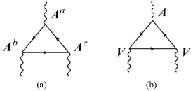
Figure 3: Anomalies can be easily detected in triangle diagrams arising in perturbation theory. The corresponding Feynman diagrams are divergent and need to be regularized. It is the regularization that breaks the classical chiral symmetry. Depending on the details of the regulator one obtains different forms of anomalies. On the right panel we show the triangle diagram for three general symmetries. One might employ a regularization scheme that treats all three vertices in a symmetric way. On the other hand in figure (b) we show the triangle leading to the axial anomaly. The $V$-vertices are singled out in that no anomaly should be associated to the $V$ vertices since they correspond to the coupling to the electromagnetic gauge field. In that case the anomaly has to be concentrated in the $A$ vertex. An alternative is to single one one particular vertex and demand that it couples covariantly to the gauge fields sitting at the other two vertices. This scheme defines the covariant anomaly.

In what follows we will describe the most general form of triangle anomalies of Dirac fields with non-Abelian symmetries and the new anomaly-induced transport phenomena associated to them. Other interesting aspects of the quantum anomalies not discussed here, including the case of (1+1) dimensional system and the topological implications of anomalies, are discussed pedagogically in Ref. Fradkin (2020)

In perturbation theory anomalies appear at one loop in the three-point function correlation functions of classically conserved currents and the energy momentum tensor (triangle diagrams, see figure 3) Adler (1969); Bell and Jackiw (1969); Kimura (1969). Alternatively they appear in the regularized definition of the path integral measure Fujikawa (1979). In four dimensions the most general form of triangle anomalies is

$$D_{\mu}J^{\mu}_{a} =\frac{d_{abc}}{32\pi^{2}}\epsilon^{\mu\nu\rho\lambda}F_{\mu\nu}^{b}F_{\mu\nu}^{c}+\frac{b_{a}}{768\pi^{2}}\epsilon^{\mu\nu\rho\lambda}R^{\alpha}\,_{\beta\rho\lambda}R^{\beta}\,_{\alpha\rho\lambda}\,,$$ (76)

$$D_{\mu}T^{\mu\alpha} =F^{\alpha\beta}_{a}J^{a}_{\beta}+\frac{b_{a}}{384\pi^{2}}\epsilon^{\mu\nu\rho\lambda}D_{\beta}\left(F_{\mu\nu}^{a}R^{\alpha\beta}\,_{\rho\lambda}\right).$$ (77)

The indices denoted by latin letters enumerate different currents $J^{\mu}_{a}$ which couple to gauge fields $A_{\mu}^{a}$. These currents can be the currents for left- and right-handed fermions, or the axial or vector like combination thereof. In general they are the Noether currents corresponding to a symmetry. The $F^{a}_{\mu\nu}$ are the field strengths of the gauge fields, $F^{a}_{\mu\nu}=\partial_{\mu}A^{a}_{\nu}-\partial_{\nu}A^{a}_{\mu}+f^{abc}A^{b}_{\mu}A^{c}_{\nu}$, where $f^{abc}$ the structure constants. The symmetries are generated by Hermitian matrices $T^{a}$ with commutation relations $[T^{a},T^{b}]=if^{abc}T^{c}$. For Abelian symmetries the structure constants vanish. The Riemann tensor $R^{\beta}\,_{\alpha\rho\lambda}$ accounts for curvature in space-time and is defined in eq. (231).

The currents and the energy-momentum tensor are composite operators in terms of the fundamental fermion fields. In quantum field theory a composite operator is one that is built out of local products of the fundamental quantum fields. For free fermions and in flat space they take the simple forms

$$J^{\mu}_{a}(x) =\bar{\Psi}_{f}(x)(T_{a})^{f}_{g}\gamma^{\mu}\Psi^{g}(x)\,,$$ (78)

$$T^{\mu\nu}(x) =\frac{i}{2}[\bar{\Psi}_{f}(x)\gamma^{(\mu}\partial^{\nu)}\Psi^{f}(x)-\partial^{(\nu}\bar{\Psi}_{f}(x)\gamma^{\mu)}\Psi^{f}(x)]\,.$$ (79)

For the Abelian vector and axial currents Eqs. (6), (7) of a Dirac fermion, $T_{a}$ is taken from $\{\mathbf{1},\gamma_{5}\}$. The round brackets on the indices denote symmetrization according to $A^{(\mu}B^{\nu)}=\frac{1}{2}(A^{\mu}B^{\nu}+A^{\nu}B^{\mu})$. Famously, quantum field theory suffers from ultraviolet divergences which must be dealt with by a regularization and renormalization scheme. In particular a composite operator is only defined up to a specific regularization scheme. The anomaly has to be understood as the fact that no regularization scheme exists which allows to realize all classical conservation laws in the quantum theory. However, different regularization schemes might give rise to different quantum definitions of the current operator. These ambiguities can be fixed by demanding certain physically plausible conditions on the currents and operators. One possible definition of regularization is to demand that the currents themselves transform as well defined tensors (”covariantly”) under the symmetry transformations even if the symmetry is anomalous. It turns out that this is a unique way of regularizing the current operators and it gives rise to what is called the covariant anomaly Bardeen and Zumino (1984). This regularization scheme is particularly well suited for answering the question if a theory does have anomalies. The anomalies in eqs. (76) and (77) are precisely these covariant anomalies. It turns out that their existence is completely determined by two simple group invariants. These are the anomaly coefficients

$$d_{abc} =\frac{1}{2}\sum_{r}\mathrm{tr}(T_{a}.\{T_{b},T_{c}\})_{r}-\frac{1}{2}\sum_{l}\mathrm{tr}(T_{a}.\{T_{b},T_{c}\})_{l}\,,$$ (80)

$$b_{a} =\sum_{r}\mathrm{tr}(T_{a})_{r}-\sum_{l}\mathrm{tr}(T_{a})_{l}\,,$$ (81)

where the sums are over the representations under which the right-handed and left-handed chiral fermions transform and curly brackets denote the anti-commutator. For a $U(1)$ symmetry, the generator $T_{a}$ in a specific representation is just as the charge $q_{a}$. The Adler-Bardeen non-renormalization theorem Adler and Bardeen (1969); Adler (2005) guarantees that there are no further quantum corrections to these numbers. The existence of anomalies can be unambiguously determined by the calculations of the anomaly coefficients $d_{abc}$ and $b_{a}$.

As an example, let us consider the single massless Dirac fermion. At the classical level a Dirac fermion is the direct sum of a right-handed and a left-handed fermion. We denote the charge of the left- and right-handed fermions by $(q_{r},q_{l})$. In a vector-axial basis we have two symmetries with charges $U(1)_{V}$: $(1,1)$ and $U(1)_{5}$: $(1,-1)$ . Accordingly the non-vanishing anomaly coefficients are $d_{5VV}=d_{V5V}=d_{VV5}=2$, $d_{555}=2$ and $b_{5}=2$. We note here that in this case all these anomaly coefficients take the same value.

Now we run however into something that appears troublesome. The anomaly coefficient $d_{abc}$ is completely symmetric, and this means that for a Dirac fermion the covariant vector current is anomalous as well

$$\partial_{\mu}J^{\mu}_{V}=\frac{1}{8\pi^{2}}\epsilon^{\mu\nu\rho\lambda}F_{\mu\nu}^{V}F_{\rho\lambda}^{5}\,.$$ (82)

This equation depends on the field strength formed by the axial gauge fields $A^{\mu}_{5}$ which couples to the axial current. One might argue that in nature there are no axial gauge fields so there is no such anomaly. This argument is however problematic. First axial gauge fields can effectively appear as happens in the low energy description of Weyl semi-metals (see Sec. VI) and secondly in a quantum theory charge conservation should be an operator equation that holds in generic correlation functions.

Since the problematic (82) is derived from (76),(77), one might ask how the anomalous conservation equation for the currents (76),(77) can be interpreted. There are at least four related but slightly different possibilities

1. First, we can interpret the anomaly equations as the non-conservation of the current corresponding to the classical symmetry $A$ when appropriate classical background gauge fields are switched on. An example is the non-conservation of axial charge in a homogeneous background of parallel electric and magnetic fields. In this case the anomaly equation becomes

   $$\dot{\rho}_{5}=\frac{1}{2\pi^{2}}\vec{E}\cdot\vec{B}\,.$$ (83)

   Axial charge is created ”out of the vacuum” at a constant rate determined by the electric and magnetic fields. Here the electromagnetic fields are thought of as external to the quantum dynamics of the Dirac fermions. In what concerns the quantum dynamics they are just classical c-numbers and not operators. This is the situation that arises in measurements of magneto conductivities of Weyl or Dirac semi-metals.

2. We can also interpret the anomaly equations as a statement of how the operator “$\partial_{\mu}J^{\mu}(x)$”, the divergence of the current or the energy momentum tensor, behaves when inserted in correlation function with other currents. Here we interpret the left-hand side of an anomaly equation as the expectation value of the divergence of the anomalous current and the right-hand side as a (local) functional of the classical sources that couple to the currents and the energy-momentum tensor. The gauge fields and the metric on the right-hand side of the anomaly equation are not physical fields but simply act as sources for insertions of the current into correlation functions according to Eqs. (32) and (39).

   As an example we consider the axial anomaly and write it as

   $$\langle\partial_{\mu}J_{5}^{\mu}(x)\rangle=\frac{1}{16\pi^{2}}\epsilon^{\mu\nu\rho\lambda}F^{V}_{\mu\nu}(x)F^{V}_{\rho\lambda}(x)\,.$$ (84)

   Functionally differentiating twice with respect the vector gauge field, i.e. applying $\frac{\delta^{2}}{\delta V_{\rho}(y)\delta V_{\lambda}(z)}$, gives the anomalous Ward identify

   $$\langle\partial_{\mu}J_{5}^{\mu}(x)J^{\nu}(y)J^{\lambda}(z)\rangle=\frac{1}{2\pi^{2}}\epsilon^{\mu\nu\rho\lambda}\partial_{\mu}^{x}\delta(x-z)\partial_{\rho}^{x}\delta(x-z)\,.$$ (85)

   This makes it clear that the anomaly appears even in the absence of physical external electric and magnetic fields as a contact term in a correlation function.

   The same logic holds for the gravitational contribution to the axial anomaly. Even in flat space the gravitational contribution to the axial anomaly does not vanish. It is manifest in correlation functions of the divergence of the axial current obtained by differentiating eq. (76) twice with respect to the metric . This type of interpretation is also often called ’t Hooft anomaly. The anomaly is not absent even if there are no gauge fields present or if one is in flat space. The external gauge fields only make the anomaly visible in the expectation value of the divergence of a current. Anomalies are properties of the quantum theory. The non-renormalization theorem also implies that the results are independent of the coupling to other matter fields. In particular anomalies are present in the free theory and can be detected by computing correlations functions of composite operators (the currents) in the free theory.

3. The anomaly can also be interpreted as an identity between two a priori different operators in a quantum field theory. This interpretation is appropriate whenever the the quantum dynamics of the gauge fields themselves is important. Whereas in the first two cases above the vacuum expectation value of the divergence of the current still vanishes if the right hand side is set to zero, this is not possible anymore if the gauge fields are dynamical. The right hand side in Eqs. (76),(77) contains now fluctuating quantum fields and therefore under no circumstance the corresponding current is really conserved. It is always subject to the quantum fluctuations of the gauge fields. Because of the quantum fluctuating gauge field there are quantum corrections to the divergence of the current due to higher-order loop diagrams, even in Abelian gauge theories Adler (2005).

4. In another situation the anomaly has to be interpreted as an inconsistency in the quantum theory. This happens when a gauge current is anomalous. What is meant here is that the current coupling to dynamical gauge fields suffers from an anomaly. This is a problem indeed. Even without quantizing the gauge fields the inconsistency can be seen from the equations of motion of a $U(1)$ gauge field

   $$\partial_{\mu}F^{\mu\nu}=J^{\nu}\,.$$ (86)

   Taking the divergence of both sides leads to an inconsistency unless the operator $\partial_{\mu}J^{\mu}$ is identically zero. This inconsistency carries over to the quantum theory and to non-Abelian gauge fields. In the quantum theory a consequence of this type of anomaly is that it would allow transverse physical photon states to scatter into unphysical longitudinal polarizations of zero norm in the Hilbert space. Thus unitarity is lost. Therefore anomalies in currents which couple to dynamical gauge fields have to vanish identically. Sometimes this can be achieved by using the ambiguities in the regularization prescription as we will exemplify below in the case of the vector like current coupling to the dynamical electro-magnetic gauge field.

These different interpretations of anomalies are often referred with specific nomenclature. For example the so-called “’t Hooft anomalies” correspond to our second point of view whereas ”ABJ anomalies” (after Adler-Bell-Jackiw) to our third point and ”gauge anomalies” to our fourth point.

Having established that anomalies can not be eliminated by going to flat space and switching off all electric and magnetic fields we still have to deal the worrisome Eq. (82). It is an anomaly in a gauge current and therefore should actually vanish. So far we have insisted that the currents transform covariantly under the symmetries even if the symmetry is anomalous. This is indeed too much to ask for. It is possible to define a vector current that is exactly conserved, even taking the axial background gauge fields into account, by changing the regularization scheme. This is the electromagnetic consistent conserved vector current. The name ”consistent” has nothing to do with the fact that this current can be consistently coupled to dynamical electromagnetic gauge fields but rather has a technical meaning in that the corresponding anomaly solves the so-called Wess-Zumino consistency conditions Wess and Zumino (1971). Without going further into details we note that (82) is a so called mixed anomaly that involves two symmetries: the axial and the vector-like ones. In such a situation of mixed anomalies it is possible to shift the consistent anomalies between the different symmetries. In particular one can completely eliminate the anomaly (82) by choosing a regularization scheme that explicitly preserves the vector-like symmetry in question (e.g. Pauli-Villars) or by adding appropriate counterterms (Bardeen counterterms) to the quantum effective action Bardeen (1969). It is however not possible to eliminate the anomaly totally. Therefore it is sufficient to calculate the symmetric anomaly coefficients $d_{abc}$ and $b_{a}$ with a covariant regularization scheme to establish the presence of anomalies. In the case of the anomaly in the vector current eq. (82) the relation of the conserved consistent current $\mathcal{J}^{\mu}$ to the covariant current $J^{\mu}$ is

$$\mathcal{J}^{\mu} =J^{\mu}-\frac{1}{4\pi^{2}}\epsilon^{\mu\nu\rho\lambda}A^{5}_{\mu}F_{\rho\lambda}\,,$$ (87)

$$\partial_{\mu}\mathcal{J}^{\mu} =0\,.$$ (88)

The additional Chern-Simons current arises from the regularization as a local finite counterterm to the current (Bardeen-Zumino Polynomial) Bardeen and Zumino (1984). The Chern-Simons current precisely cancels the anomaly in the covariant current. Note that this also means that now the axial gauge field is not really a gauge field anymore. It is a physical field and observable as a current in electric and magnetic fields. This conserved consistent current can now be coupled to a Maxwell field and has a good physical interpretation as electric current. On the other hand the anomaly in the axial current can not be cancelled in the same way since it contains the term

$$\partial_{\mu}J^{\mu}_{5}=\dot{\rho}_{5}+\vec{\nabla}\cdot\vec{J}_{5}=\frac{1}{16\pi^{2}}\epsilon^{\mu\nu\rho\lambda}F^{V}_{\mu\nu}F^{V}_{\rho\lambda}=\frac{1}{2\pi^{2}}\vec{E}\cdot\vec{B}\,.$$ (89)

The corresponding Chern-Simons current that would cancel this anomaly depends explicitly on the (true) electromagnetic gauge field $V_{\mu}$ and thus has to be considered unphysical. The axial anomaly is there because of the non-zero $d_{VVA}$ coefficient. We note that also the $d_{AAA}$ coefficient is non-vanishing. This essentially means that the axial symmetry is hopelessly lost in the quantum theory. Therefore the best possible result is that the vector-like symmetry is preserved in the quantum theory. The corresponding consistent current is conserved and can be interpreted as electric current.

In the case of the gravitational anomaly the covariant form indeed makes the energy-momentum tensor a non-conserved current. But again one can add counterterms to the quantum effective action which cancel the anomaly in the energy-momentum tensorBardeen (1969); Alvarez-Gaume and Witten (1984). In theory one could also keep the anomaly in the energy-momentum tensor and cancel the anomaly in the axial current, but it is not possible to keep the conservation laws for both of them simultaneously.

V.2 Anomalies in matter

Now we discuss anomaly induced transport, in particular the so-called chiral magnetic and chiral vortical effects Vilenkin (1979, 1980); Alekseev et al. (1998); Giovannini and Shaposhnikov (1998); Newman (2006); Fukushima et al. (2008); Son and Surowka (2009); Erdmenger et al. (2009); Banerjee et al. (2011). The chiral magnetic effect (CME) denotes the generation of a current in parallel to an applied magnetic field $\vec{B}$ and the chiral vortical effect (CVE) is the generation of a current along a vortex $\vec{\Omega}$ (for a review see Landsteiner (2016); Kharzeev (2014),).

$$\vec{J}_{a} =\sigma_{ab}\vec{B}_{b}+\sigma^{\Omega}_{a}\vec{\Omega}\,,$$ (90)

$$\vec{J}_{\epsilon} =\sigma_{a}^{\epsilon}\vec{B}_{a}+\sigma^{\epsilon,\Omega}\vec{\Omega}\,.$$ (91)

The gauge fields are not necessarily physical fields but can simply be sources for the currents as outlined before. The vorticity is $\vec{\Omega}=\frac{1}{2}\vec{\nabla}\times\vec{v}$. Explicit calculations in free fermion theories Landsteiner et al. (2011a) and in holographic field theories Landsteiner et al. (2011b) give the results

$$\sigma_{ab} =\frac{d_{abc}\mu_{C}}{4\pi^{2}}\,,$$ (92)

$$\sigma_{a}^{\Omega} =\frac{d_{abc}\mu_{b}\mu_{c}}{4\pi^{2}}+\frac{b_{a}}{12}T^{2}\,,$$ (93)

$$\sigma_{a}^{\epsilon} =\frac{d_{abc}\mu_{b}\mu_{c}}{8\pi^{2}}+\frac{b_{a}}{24}T^{2}\,,$$ (94)

$$\sigma^{\epsilon,\Omega} =\frac{d_{abc}\mu_{a}\mu_{b}\mu_{c}}{12\pi^{2}}+\frac{b_{a}\mu_{a}}{12}T^{2}$$ (95)

The remarkable fact is that these transport coefficients are completely determined by the anomaly coefficients (80) and (81). It means that these currents are non-zero when the theory has the anomalies (82). Since anomalies are subject to non-renormalization theorems one expects non-renormalization theorems to hold for these transport coefficients as well. Perturbative proofs of non-renormalization have been presented in Golkar and Son (2015); Hou et al. (2012).

It is important to realize that these non-renormalization theorems hold only when the gauge fields on the right hand side of the anomaly equation are non-dynamical classical fields (’t Hooft anomalies). On the other hand if the gauge fields are taken as quantum fields (ABJ anomalies) as well they give rise to non-trivial loop corrections. This was first pointed out in Hou et al. (2012) for the $T^{2}$ terms and later shown to hold for all chiral conductivities (92)-(95) in Jensen et al. (2013a). In hindsight this is not surprising since also the divergence of an anomalous current is renormalized in this situation Adler (2005). The non-renormalization properties of the chiral conductivities are therefore the same as the ones of the anomalous divergence of the current itself.

The dependence on the chemical potentials in Eqs. (92) - (95) is also fixed by demanding the existence of an entropy current with positive divergence (generalized second law) Son and Surowka (2009); Neiman and Oz (2011) in the presence of chiral anomalies. The dependence on the temperature on the other hand can not be fixed by this criterion. Rather the temperature enters as an integration constant Neiman and Oz (2011). More advanced consideration are necessary to establish a general relation between the gravitational contribution to the anomalies and the temperature dependence in (93)-(95). This has first been established in Jensen et al. (2013b). The approach of Jensen et al. (2013b) was to study Euclidean quantum field theory on cone-like geometries. A related setup this time however in a Lorentzian signature space-time containing a black hole was developed in Stone and Kim (2018). This involves integration of the anomaly equations (76), (77) in a black-hole space time with the boundary condition such that the currents and the energy current vanish on the horizon. We will briefly review this argument in the Appendix E. Finally the relation of the temperature dependence of the anomalous transport coefficients to a global version of gravitational anomaly has been established in Golkar and Sethi (2016) and further studied in Chowdhury and David (2016); Glorioso et al. (2019).

It might come as a surprise that the gravitational contribution to the chiral anomaly can enter the chiral conductivities. One should keep in mind that the theory is anomalous even in flat space, in the absence of gauge fields and without interactions. It still is somewhat surprising since the gravitational anomaly is a term of fourth order in derivatives and naively can not influence terms in transport that are only first order. It is certainly true that in vacuum one can not form candidate covariant terms of lower degree in derivatives. In vacuum the only available tensor is the metric and there exists no covariant tensor that can be formed with only one derivative on the metric. The chiral transport expression apply however not in vacuum but in a gapless theory of chiral fermions at finite temperature and chemical potential. This means that in the low energy theory one has more effective fields, not only the metric or the gauge fields but also the effective low energy fields temperature $T(x)$, chemical potential $\mu(x)$ and the velocity field $u^{\mu}(x)$. This allows now to form new covariant objects, such as the vorticity $\Omega^{\mu}$ with low degrees of derivatives. We have emphasized in section III that temperature and velocity variations have the same effect in local thermal equilibrium as variations in the gravitational background. This gives an intuitive reason why gravitational effects can be captured by temperature and vorticity. In particular if a gravito-magnetic field (see Appendix D) is present as a small perturbation of otherwise flat space-time $\delta g_{ti}=A^{g}_{i}$, even a fluid at rest $u^{\mu}=(1,0,0,0)$ can have vorticity $2\vec{\Omega}=\vec{B_{g}}=\vec{\nabla}\times\vec{A}^{g}$. The vorticity is induced via frame dragging by the gravito-magnetic potential $\vec{A}_{g}$. In this sense the chiral vortical effect can also be seen as a chiral gravito-magnetic effect Landsteiner et al. (2011c).

As already mentioned the anomaly induced conductivities (92) - (95) are also constrained by a generalized second law of thermodynamics. It is possible to define an entropy current such that the anomalous currents do not contribute to entropy production. This anomalous contribution to the entropy current is given by Son and Surowka (2009); Neiman and Oz (2011); Stephanov and Yee (2016)

$$\vec{J}_{S,\mathrm{anom}}=\frac{T}{12}b_{a}\vec{B}_{a}+\frac{\mu_{a}b_{a}}{6}\vec{\Omega}$$ (96)

Later we will show that using this expression one can derive the Wiedemann-Franz law and the Mott formula for anomalous transport in Weyl semimetals by defining an appropriate heat current based on this entropy current as $J^{\mu}_{Q}=TJ^{\mu}_{S}$. For clarity let us emphasize that we have not considered dissipative transport here. Including also dissipative transport coefficients the total entropy current fulfills $\partial_{\mu}J_{S}^{\mu}\geq 0$.

We note that the expression for the entropy current (96) depends also on the frame choice. The one quoted here corresponds to the so-called ”no-drag” frame Stephanov and Yee (2016). This is the frame in which the fluid is at rest for $u^{\mu}=U^{\mu}$ and $U^{\mu}$ denotes the frame field of a impurities on on which the fluid looses momentum. In a condensed matter context there are always impurities which imply the existence of a preferred frame. For applications of anomalous transport to condensed matter physics the no-drag frame is therefore the physically preferred one.

A violation of the relation between triangle anomalies and the chiral vortical effect happens for relativistic spin $3/2$ fermions (gravitinos) Loganayagam and Surowka (2012). In that case it was shown in Golkar and Sethi (2016) that a global version of the gravitational anomaly implies the chiral vortical effect (see also Chowdhury and David (2016); Glorioso et al. (2019)). Finally we point out that recently the relation between the gravitational anomaly in Maxwell theory and a photonic analogue of the chiral vortical effect has been shown to hold if both are calculated with the same regulator Prokhorov et al. (2020).

V.3 Anomalies and magnetotransport in Weyl semi-metals

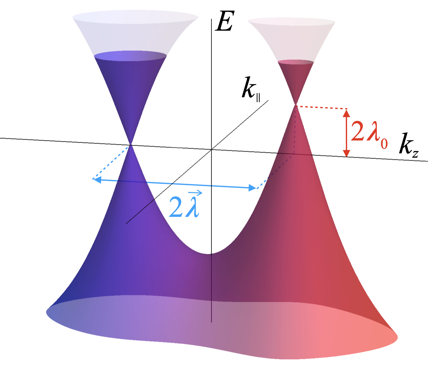
Figure 4: A schematic view of a Weyl semimetal’s band structure.

In Figure 4 we show a schematic view of the band structure of a Weyl semi-metal. In this simple description, the band structure has two band crossing points near the Fermi level. By the Nielsen-Ninomiya theorem the two nodal points have opposite chirality. To lowest order in a derivative expansion near the Fermi points, the electronics can be effectively described by two Weyl fermions of opposite chirality. A useful equivalent view is to combine both Weyl fermions into one Dirac fermion. Then the Dirac like wave equation for this four-component spinor is Zyuzin et al. (2012); Grushin (2012); Zyuzin and Burkov (2012); Goswami and Tewari (2013)

$$(i\gamma^{\mu}\partial_{\mu}+\gamma^{\mu}\lambda_{\mu}\gamma_{5})\psi=0\,.$$ (97)

The four vector $\lambda_{\mu}=(\lambda_{0},\vec{\lambda})$ describes the separation of the Weyl nodes of opposite chirality in momentum space. A useful view is to consider $\lambda_{\mu}$ to be the background value of an axial gauge field $A_{\mu}^{5}=\lambda_{\mu}$. As we have already emphasized the description in terms of chiral fermions in a crystal is not exact. Due to the compactness of the Brillouin zone the bands hosting left- and right-handed chiral fermions are connected such that a hard scattering process might scatter a fermionic quasiparticle from one Weyl cone to another one of opposite chirality. This inter-valley scattering will have as a consequence that in equilibrium the Fermi energies of left- and right-handed Weyl cones are equal $\epsilon_{F}^{R}=\epsilon_{F}^{L}=\epsilon_{F}$. In order to apply the quantum field theoretical transport formulas we need to measured energies with respect to the normal ordered vacuum. This is defined with respect to the band crossing points at which the density of states within a Weyl cone vanishes. Let us denote these points with $(E_{R,L},\vec{K}_{R,L})$. We can define now the four vector $\lambda_{\mu}$ by $(\lambda_{0},\vec{\lambda})=\frac{1}{2}(E_{R}-E_{L},\vec{K}_{R}-\vec{K}_{L})$. In particular the chemical potentials have to be measured relative to the locations of the Weyl points such that $\mu_{R,L}=\epsilon_{F}-E_{R,L}$. The total chemical potential is $\mu=\frac{1}{2}(\mu_{R}+\mu_{L})$. For the axial chemical potential we have $\mu_{5}=\frac{1}{2}(\mu_{R}-\mu_{L})=\lambda_{0}$ in equilibrium.

We now review how the anomalous transport formulas lead to a theory of magneto-transport in Weyl semi-metals. First we want to get the so called Bloch theorem out of our way. Bloch argued that a system can not sustain an electric current in thermal equilibrium. As we briefly reviewed in the introduction, the Bloch theorem applies only to currents which are exactly conserved gauge currents. Thus we need not be concerned about currents that are not gauge currents, e.g. the axial current $J_{5}^{\mu}$ can have an equilibrium expectation value without being in conflict with Bloch’s argument. This applies to the so-called Chiral Separation Effect (CSE)

$$\vec{J}_{5}=\frac{\mu}{2\pi^{2}}\vec{B}\,.$$ (98)

It is a special case of the general anomaly transport formulas (90) with $d_{5VV}=2$. More worrisome is the expression

$$\vec{J}=\frac{\mu_{5}}{2\pi^{2}}\vec{B}\,,$$ (99)

the Chiral Magnetic Effect proper. In this form it is determined by the same totally symmetric anomaly coefficient $d_{5VV}$. Again it simply is a special case of eq. (90). If we were to interpret the current in eq. (99) as electric current it would contradict the Bloch theorem. Since the Bloch theorem is a consequence of gauge invariance it would also indicate a subtle violation of gauge symmetry. We need to remember however, that there is an ambiguity in the definition of the current and we need to make sure that we actually use the properly defined quantum operator. The electric current should be conserved under all circumstances. Therefore it is correct to identify the conserved consistent current (87) as electric current with the identification $A^{5}_{\mu}=\lambda_{\mu}$! This conserved consistent current has an additional contribution stemming from the Chern-Simons current. The Bloch theorem can be expected to hold only for the conserved consistent current $\mathcal{J}^{\mu}$. If we add this contribution we find

$$\vec{\mathcal{J}}=\frac{\mu_{5}-\lambda_{0}}{2\pi^{2}}\vec{B}\,.$$ (100)

As we explained before in equilibrium we have the relation $\lambda_{0}=\mu_{5}$ and thus the Bloch theorem is obeyed. The chiral magnetic current vanishes identically in strict equilibrium. This result has first been obtained in a holographic calculation Rebhan et al. (2010); Gynther et al. (2011). In Gynther et al. (2011) it was also shown that it is a consequence of any gauge invariant regularization in quantum field theory. Later it was shown to hold in a tight-binding approach in Vazifeh and Franz (2013) which from the point of view of quantum field theory can be viewed as a lattice regularization. The presence of the Chern-Simons term in a tight binding approach has been explicitly calculated in Gorbar et al. (2017b). The identification of consistent and covariant currents in lattice models becomes more involved in the presence of axial gauge fields Behrends et al. (2019). These issues arise if one seeks a quantum field theoretical description. However, this is not strictly necessary as momentum-space in a crystal is compact. So, instead of doing quantum field theory with a normal ordered vacuum, one might just do many body quantum mechanics an measure energies with respect to the bottom of the band. This point of view has been emphasized in Refs. Basar et al. (2014); Behrends et al. (2019). In any case it is re-assuring that both points of view give rise to the same results.

Since we can not expect to get any measurable effect by simply applying a magnetic field to a Weyl semi-metal we need to do something more to drive the system slightly out of equilibrium. To activate the CME we must break the relation $\mu_{5}=\lambda_{0}$ in some way. Here it is important that the chemical potential is a state variable whereas the axial gauge field is an external parameter. The quantum dynamics of the fermions alone can not change it the external field $A^{5}_{0}=\lambda_{0}$ but only the state variable $\mu_{5}$. If we do work on the fermions we can change their state, e.g. applying an electric field leads to an increase of temperature due to Joule heating. In an analogous way the anomalous transport phenomena have an impact on the state of the fermionic system and can drive them out of equilibrium leading to measurable electric and heat currents.

We may imagine injecting electrons at one end of a Weyl semi-metal and extracting fermions on the other side. This will effectively lead to a gradient in the chemical potential $\vec{\nabla}\mu$. Alternatively we can apply an electric field $\vec{E}$. Now we use the anomalous conservation of the axial current (89) to obtain the increase in axial charge

$$\dot{\rho}_{5}=\frac{1}{2\pi^{2}}\vec{E}\cdot\vec{B}-\vec{\nabla}\cdot\vec{J}_{5}=\frac{1}{2\pi^{2}}(\vec{E}-\nabla\mu)\cdot\vec{B}\,.$$ (101)

We also have taken into account the contribution of the CSE current eq. (98) proportional to the chemical potential. Now we relate the axial charge density to the axial chemical potential via an axial susceptibility $\chi_{5}=\partial\rho_{5}/\partial\mu_{5}$

$$\dot{\rho}_{5}=\chi_{5}\cdot\mu_{5}\,.$$ (102)

Fourier transforming in time leads to an increase in the axial chemical potential away from its equilibrium value

$$\delta\mu_{5}=i\frac{(\vec{E}-\vec{\nabla}\mu)\cdot\vec{B}}{2\pi^{2}\chi_{5}\omega}\,.$$ (103)

Since we are interested in a steady state situation we have to take the limit $\omega\rightarrow 0$ in which the axial charge diverges. In a crystal axial charge is however destroyed due to large momentum scatterings from one Weyl cone into the other. This takes place at a time scale $\tau_{5}$ which is called the inter-valley scattering time Son and Spivak (2013). This is also the time scale at which the growth of the axial chemical potential will be cut off. Formally this can be represented by the substitution.

$$\omega\rightarrow\omega+i/\tau_{5}\,,$$ (104)

with $\tau_{5}$ the inter-valley scattering time. In this way one predicts a finite value of the axial chemical potential which eventually can be plugged into the formula for the CME to obtain

$$\vec{J}=\tau_{5}\frac{(\vec{E}-\vec{\nabla}\mu)\cdot\vec{B}}{4\pi^{4}\chi_{5}}\vec{B}\,.$$ (105)

This reasoning predicts a large enhancement of the electric conductivity in a magnetic field if the inter valley scatting time is a long time scale Nielsen and Ninomiya (1983b); Li et al. (2016). A microscopic calculation in a kinetic theory approach was presented in Son and Spivak (2013). Here we have emphasized that it is based on universal results, anomalous conservation laws and the corresponding anomaly induced transport phenomena. We also made it clear that even when there are no external electric fields the effect can be triggered by driving the system in a state with a gradient in the chemical potential. This is just a reflection of the well known fact that in linear response the effect of an electric field is the same as the effect of a gradient in the chemical potential.

V.4 Anomaly induced magneto-electric and -thermal transport for Weyl semi-metals 

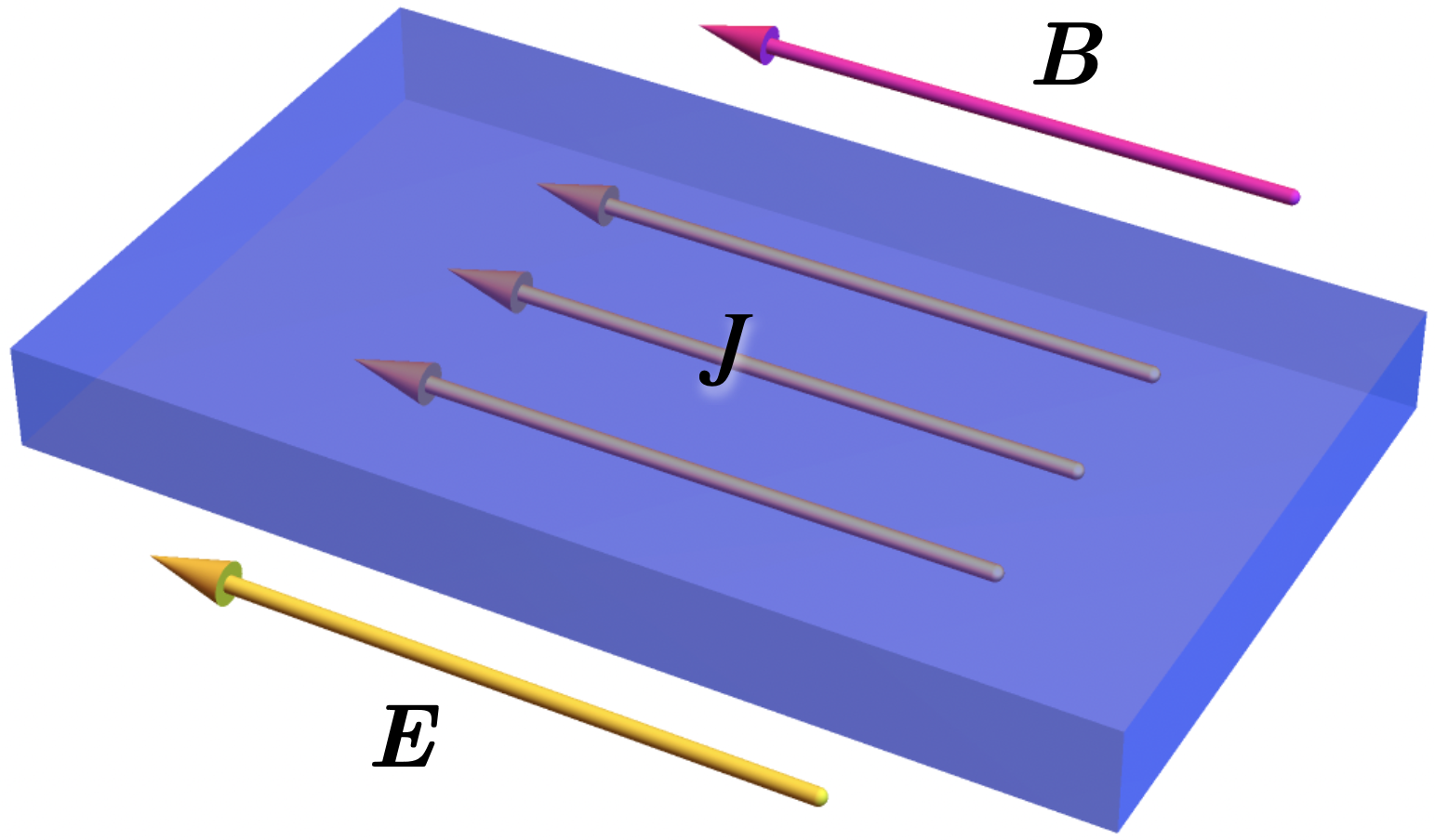
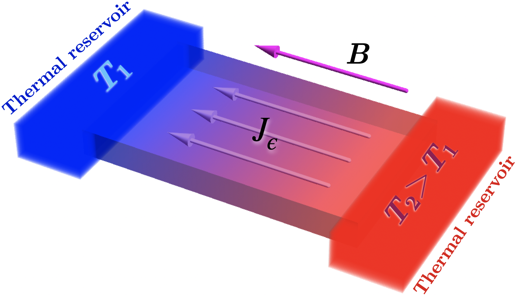
(a)	(b)

Figure 5: Schematics of the enhanced transport in an magnetic field due to anomalies. In panel (a) in addition to the magnetic field a parallel electric field is applied. This leads to an enhanced current due to the chiral magnetic effect. In panel (b) a temperature gradient parallel to the magnetic field activates the temperature component of the chiral magnetic effect in the energy current (see Eq. (94)) proportional to the gravitational anomaly coefficient.

Let us now discuss anomaly induced magneto-electric and -thermal transport for Weyl semi-metals (see Figure 5). This can and has been studied in a microscopic approach based on (chiral) kinetic theory and the corresponding Boltzmann equation Spivak and Andreev (2016); Lundgren et al. (2014). The relation of the thermal conductivities to the anomalies is however not evident in such an approach. In contrast, the effective transport theory based on the anomalous transport currents Eqs. (92)-(95), can track the anomaly contribution. This has been shown first in a hydrodynamic model in Lucas et al. (2016). It is however unclear if a hydrodynamic regime with independent flow for different chiralities can be achieved in a Weyl semi-metal. Fortunately, an effective theory of coupled charge and energy transport in a magnetic field based on anomaly induced transport can be developed without assuming a hydrodynamic regime, as we will review now.

First, we elaborate on the role played by the different relaxation processes. In general we can distinguish between intravalley, intervalley and electron-electron or electron-phonon scattering. A key assumption is that there exists a hierarchy of relaxation times $\tau<\tau_{5}<\tau_{ee}\approx\tau_{e\phi}$. The intravalley scattering time $\tau$ is the shortest. It is the timescale in which electronic particles are scattered but the change is their momentum is small such that they stay within the same Weyl cone in momentum space. This scattering distributes the electronic quasiparticles randomly in the phase space corresponding to a single Weyl cone. Second, we assume an inter-valley scattering time scale $\tau_{5}$. It is supposed to be significantly longer than $\tau$. Finally we also assume that electron-electron and electron-phonon interactions are even rarer than inter-valley scattering events. Note that these assumptions exclude hydrodynamic behavior of the electrons. Formally we will work with an idealized situation in which $\tau=0$ and $\tau_{ee},\tau_{e\phi}=\infty$. That means that momentum is not a relevant low energy degree of freedom whereas the energies and charges of each individual Weyl cone are approximately conserved, on a time scale given by the intervalley scattering time $\tau_{5}$.

To set up an effective transport model we concentrate on the charges conserved by the fast elastic intravalley scattering. These are the energy and charge densities. A transport theory should include temperatures and chemical potentials for each Weyl cone. It corresponds to the quantum numbers that are conserved up to a timescale of order $\tau_{5}$. In the absence of external driving forces the temperatures and chemical potentials will equilibrate at times longer than $\tau_{5}$.

The currents induced by the anomalies are dissipationless and therefore we expect them to be insensitive to momentum relaxing elastic scattering. Indeed model calculations in holography Copetti et al. (2017) and in a hydrodynamic setup Stephanov and Yee (2016) have shown anomalous transport formulas to be robust against momentum relaxation. In a quasi-particle picture the robustness of anomalous transport can be argued on the grounds that the anomalous transport stems from the lowest Landau level. Then we can view the relevant degrees of freedom as $1+1$ dimensional chiral fermions which naturally suppresses backscattering.

We base our treatment on anomalous transport of right- and left-handed fermions in a magnetic field. The corresponding symmetry is the vector-symmetry $U(1)_{V}=U(1)_{L}\otimes U(1)_{R}$. The magnetic field acts on both chiralities in the same way.

The anomaly coefficients determining the chiral currents in a magnetic field are therefore $d_{LLV}$, $d_{RRV}$, $b_{L}$ and $b_{R}$ defined in eqs. (76),(77). Due to the Nielsen-Ninomiya theorem the number of left-handed Weyl cones has to be equal to the number of right-handed Weyl cones ($n_{R}=n_{L}$). Under the left-right symmetry $U(1)_{L}\otimes U(1)_{R}$ the left-handed fermions have charges $(1,0)$ whereas the right-handed fermions have charge $(0,1)$. The anomaly coefficients are then

$$d_{RRV}=-d_{LLV}=b_{R}=-b_{L}=1\,.$$ (106)

for a single Weyl cone depending on its chirality. The Nielsen-Ninomiya theorem guarantees that the vector symmetry is anomaly free, i.e. $d_{VVV}=b_{V}=0$. Due to this simple structure it is sufficient to consider only one Weyl cone. The total current can be obtained by summing over the currents from each Weyl cone.

The anomaly induced energy and charge currents in a magnetic field in a single Weyl cone are

$$\vec{J}^{\epsilon}_{L,R} =\pm\left(\frac{\mu^{2}}{8\pi^{2}}+\frac{T^{2}}{24}\right)\vec{B}\,,$$ (107)

$$\vec{J}_{R,L} =\pm\frac{\mu}{4\pi^{2}}\vec{B}\,.$$ (108)

The sign is determined by the anomaly coefficients (106). These expression are obtained from (90) and (91) by going to the restframe $u^{\mu}=(1,0,0,0)$ and identifying the energy current as $T^{0i}=J_{\epsilon}^{i}$. Now we want to study the effect of applying an external electric field (or a gradient in the chemical potential) and a thermal gradient to the system. Because the anomaly acts on each Weyl cone we find from anomalous current conservation

$$\delta\dot{\epsilon} =-\vec{\nabla}\cdot\vec{J}_{\epsilon}+\vec{E}\cdot\vec{J}\,,$$ (109)

$$\delta\dot{\rho} =-\vec{\nabla}\cdot\vec{J}\pm\frac{1}{4\pi^{2}}\vec{E}\cdot\vec{B}\,.$$ (110)

The first line is energy conservation taking into account the Joule-heating term and the second line is the anomalous conservation law of the number density of Weyl fermions in a single cone. Using Eqs. (107) and (108) allows to compute the growth rates of energy and number densities in a single Weyl cone as

$$-i(\omega+\frac{i}{\tau_{5}})\delta\epsilon =\mp\left(\frac{\mu}{4\pi^{2}}(\vec{\nabla}\mu-\vec{E})\cdot\vec{B}+\frac{T}{12}\vec{\nabla}T\cdot\vec{B}\right)\,,$$ (111)

$$-i(\omega+\frac{i}{\tau_{5}})\delta\rho =\mp\frac{1}{4\pi^{2}}(\vec{\nabla}\mu-\vec{E})\cdot\vec{B}\,.$$ (112)

We also have already performed a Fourier transform in time. As before we cut off the infinite growth at zero frequency by the intervalley relaxation time. This allows us to simply set $\omega=0$ and compute $\delta\epsilon$ and $\delta\rho$. Now we express the energy and number densities by the chemical potentials using the susceptibility matrix $\chi$

$$\left(\begin{array}[]{c}\delta\epsilon\\ \delta\rho\end{array}\right)=\chi\cdot\left(\begin{array}[]{c}\delta T\\ \delta\mu\end{array}\right),$$ (113)

where

$$\chi=\left(\begin{array}[]{cc}\frac{\partial\epsilon}{\partial T}&\frac{\partial\epsilon}{\partial\mu}\\ \frac{\partial\rho}{\partial T}&\frac{\partial\rho}{\partial\mu}\end{array}\right).$$ (114)

We can plug these increments of the temperatures and chemical potentials into the anomaly induced currents

$$\delta\vec{J}^{\epsilon} =\pm\left(\frac{\mu\delta\mu}{4\pi^{2}}+\frac{T}{12}\delta T\right)\vec{B}\,,$$ (115)

$$\delta\vec{J} =\pm\frac{1}{4\pi^{2}}\delta\mu\vec{B}\,.$$ (116)

Finally we can put everything together and compute the induced energy and charge current for each single Weyl cone. In matrix notation it is conveniently expressed as

$$\left(\begin{array}[]{c}\delta J^{\epsilon}_{i}\\ \delta J_{i}\end{array}\right) =\Sigma_{ij}\cdot\left(\begin{array}[]{c}-\partial_{j}T\\ E_{j}-\partial_{j}\mu\end{array}\right)\,,$$ (121)

$$\Sigma_{ij} =\tau_{5}\left(\begin{array}[]{cc}\frac{T}{12}&\frac{\mu}{4\pi^{2}}\\ 0&\frac{1}{4\pi^{2}}\end{array}\right)\cdot\chi^{-1}\cdot\left(\begin{array}[]{cc}\frac{T}{12}&\frac{\mu}{4\pi^{2}}\\ 0&\frac{1}{4\pi^{2}}\end{array}\right)B_{i}B_{j}\,.$$ (126)

The final result does not depend on the chirality. Both chiralities contribute in the same way.

V.5 Weak magnetic field

Let us apply this result now to a gas of free chiral fermions. We also assume here that the magnetic field is small compared to chemical potential $\mu$ and and temperature $B$, i.e. $B/T^{2}\ll 1$ and $B/\mu^{2}\ll 1$. The free energy density is Le Bellac (2000)

$$F=-\frac{1}{24\pi^{2}}\left(\mu^{4}+2\pi^{2}T^{2}\mu^{2}+7/15\pi^{4}T^{4}\right),$$ (127)

from which the energy $\epsilon=F-\frac{\partial F}{\partial T}+\mu\rho$ and the number density $\rho=-\frac{\partial F}{\partial\mu}$ and the  susceptibility matrix $\chi$ can be calculated. The conductivity matrix as defined in (121) is

$$\Sigma_{ij}=\left(\begin{array}[]{cc}\kappa_{ij}&\beta_{ij}\\ \alpha_{ij}&\sigma_{ij}\end{array}\right),$$ (128)

where the different entries are the anomaly induced contributions to the different conductivities

$$\mathrm{thermal~{}conductivity}:\kappa_{ij} =\tau_{5}B_{i}B_{j}\frac{15\mu^{2}T-5\pi^{2}T^{3}}{24\Delta}$$ (129)

$$\mathrm{electro-thermal~{}conductivity}:\beta_{ij} =\tau_{5}B_{i}B_{j}\frac{11\pi^{2}T^{2}\mu+15\mu^{3}}{8\pi^{2}\Delta}$$ (130)

$$\mathrm{thermo-electric~{}conductivity}:\alpha_{ij} =-\tau_{5}B_{i}B_{j}\frac{5\mu T}{4\Delta}$$ (131)

$$\mathrm{electric~{}conductivity}:\sigma_{ij} =\tau_{5}B_{i}B_{j}\frac{21\pi^{2}T^{2}+15\mu^{2}}{8\pi^{2}\Delta}\,,$$ (132)

with $\Delta=7\pi^{4}T^{4}+6\pi^{2}T^{2}\mu^{2}+15\mu^{4}$.

V.6 Thermoelectric transport relations of the anomaly-induced transport coefficients

We will now study how the anomaly induced conductivities collected in the matrix $\Sigma_{ij}$ realize some standard electronic transport properties such as the Onsager reciprocity relation, the Wiedemann-Franz law and the Mott relation. Let us start with the Onsager reciprocity relations.

• Onsager relations. They are a consequence of time-reversal symmetry and should hold on general grounds. We note that the magnetic field breaks time-reversal symmetry which means that Onsager’s relations hold if one replaces $\vec{B}\rightarrow-\vec{B}$. The anomaly induced conductivity matrix $\Sigma_{ij}$ is however quadratic in the magnetic field and therefore insensitive to the sign of the magnetic field. The conductivity matrix $\Sigma_{ij}$ is the response due to gradients in temperature, chemical potential and electric field. Onsager relations are manifest however if the conductivities are written as responses due to gradients in the thermodynamic driving forces (Langrange multipliers) $\beta=1/T$ and $\gamma=-\mu/T$. The Onsager reciprocity relations state then that the conductivity matrix should be symmetric and positive. By transforming to the $\beta$, $\gamma$ basis

  $$\left(\begin{array}[]{c}J^{\epsilon}_{i}\\ J_{i}\end{array}\right) =L_{ij}\cdot\left(\begin{array}[]{c}\partial_{j}(\frac{1}{T})\\ \frac{E_{j}}{T}-\partial_{j}(\frac{\mu}{T})\end{array}\right),$$ (137)

  and we find

  $$L_{ij} =\Sigma_{ij}\cdot\left(\begin{array}[]{cc}T^{2}&0\\ \mu T&T\end{array}\right)=\frac{\tau_{5}B_{i}B_{j}}{\Delta}\left(\begin{array}[]{cc}\frac{1}{24\pi^{2}}(5\pi^{4}T^{5}+18\pi^{2}T^{3}\mu^{2}+45T\mu^{4})&\frac{T\mu}{8\pi^{2}}(11\pi^{2}T^{2}+15\mu^{2})\\ \frac{T\mu}{8\pi^{2}}(11\pi^{2}T^{2}+15\mu^{2})&\frac{3T}{8\pi^{2}}(7\pi^{2}T^{2}+5\mu^{2})\end{array}\right),$$ (142)

  which is indeed symmetric and positive definite.
  

• Wiedemann-Franz law and the Lorentz-ratio from anomalies. One of the basic paradigms of quasiparticle transport is the Wiedemann-Franz law. It states that at low temperature the ratio of the thermal conductivity for the heat current and the electric conductivity is given by a constant, the Lorenz number $L=\pi^{2}k_{B}^{2}/(3e^{2})$ times the temperature $T$. Here we sill show that also the anomaly induced magnetoconductivities of a chiral fermion obey the Wiedemann-Franz law. Let us define the heat current by

  $$\vec{J}_{Q}=\vec{J}^{\epsilon}-\mu\vec{J}$$ (143)

  where we use the currents from eq. (121). The thermal conductivity in the heat current is defined by

  $$J_{Q,i}=-\hat{\kappa}_{ij}\partial_{j}T$$ (144)

  Alternatively we could use the definition of the anomaly induced entropy current (96). Note that the net entropy current in equilibrium vanishes since the contributions form left-handed and right-handed Weyl fermions cancel. But upon applying the temperature gradient and electric field they are shifted out of their equilibrium values as in (113). In particular the increment in temperature is

  $$\delta T=\mp\tau_{5}\frac{5\pi^{2}T^{3}+15\mu^{2}T}{2\Delta}\vec{B}.\vec{\nabla}T\,.$$ (145)

  Using this expression for the entropy current

  $$J_{S,i}=\pm\frac{\delta T}{12}B_{i}=-\tau_{5}\frac{5\pi^{2}T^{3}+15\mu^{2}T}{24\Delta}B_{i}B_{j}\partial_{j}T\,.$$ (146)

  From this expression for the anomaly induced entropy current we can give another definition of heat current as

  $$\vec{J}_{Q}=T\vec{J_{S}}\,.$$ (147)

  While the two definitions of heat current look very different the do indeed give the same result eq. (146)!

  Now we can build the ratio of the diagonal parts of the thermal and electric conductivities (we also restore the Boltzmann constant $k_{B}$ and the unit of electric charge $e$)

  $$\frac{\hat{\kappa}_{ii}}{\sigma_{ii}}=\frac{5k_{B}^{2}\pi^{2}(\pi^{2}k_{B}^{2}T^{3}+3\mu^{2}T)}{e^{2}9(7\pi^{2}k_{B}^{2}T^{2}+5\mu^{2})}=\frac{\pi^{2}k_{B}^{2}}{3e^{2}}T+O(T^{2}/\mu^{2})\,.$$ (148)

  To leading order in $\mu/T$ this expression gives the usual Lorenz ratio. The anomaly induced magnetic conductivities fulfil the Wiedemann-Franz law in the regime of small temperature and large chemical potential.
  

• Seebeck coefficient and Mott formula. The Seebeck coefficient describes how much voltage is built up when applying a temperature gradient at vanishing electric current. From

  $$0=\vec{J}=\sigma\vec{E}-\alpha\vec{\nabla}T\,.$$ (149)

  we see that the Seebeck coefficient $S$ is the ratio of the thermo-electric conductivity and the electric conductivity. Again we consider for simplicity only the diagonal parts describing the conductivities along with the magnetic field

  $$S=\frac{\sigma_{ii}}{\alpha_{ii}}\,.$$ (150)

  At large chemical potential the Mott formula states that

  $$S=-\frac{\pi^{2}k_{B}^{2}T}{3e}\frac{dc(\mu)/d\mu}{c(\mu)}~{}~{},~{}~{}\sigma(\mu,T)=c(\mu)+O(T^{2}/\mu^{2})\,.$$ (151)

  Again we insert the electric charge unit and the Boltzmann constant as before. To leading order in $\mu/T$ from Eqs. (131) and (132) we find

  $$c(\mu) =\frac{e^{2}\tau}{8\pi^{2}\mu^{2}}\,,$$ (152)

  $$S =-\frac{2k_{B}^{2}\pi^{2}T}{3e\mu}$$ (153)

  which indeed fulfills the Mott formula.

V.7 Large magnetic field

So far we have assumed that the magnetic field is small. In the quantum regime, in which the magnetic field sets the dominant energy scale $B\gg T^{2}$, $B\gg\mu^{2}$ we may assume that all fermions are in the lowest Landau level. The free energy is now

$$F=-\frac{|B|}{24\pi^{2}}(\pi^{2}T^{2}+3\mu^{2})\,.$$ (154)

Going through he same considerations as before we find the conductivity matrix $\Sigma$ with the entries

$$\Sigma_{ij}=\frac{\tau_{5}}{4\pi^{2}|B|}\left(\begin{array}[]{cc}\frac{\pi^{2}T}{3}&\mu\\ 0&1\end{array}\right)B_{i}B_{j}$$ (155)

$$\mathrm{thermal~{}conductivity}:\kappa_{ij} =\tau_{5}\frac{B_{i}B_{j}}{|B|}\frac{T}{12}$$ (156)

$$\mathrm{electro-thermal~{}conductivity}:\beta_{ij} =\tau_{5}\frac{B_{i}B_{j}}{|B|}\frac{\mu}{4\pi^{2}}$$ (157)

$$\mbox{thermo-electric conductivity}:\alpha_{ij} =0$$ (158)

$$\mathrm{electric~{}conductivity}:\sigma_{ij} =\tau_{5}\frac{B_{i}B_{j}}{|B|}\frac{1}{4\pi^{2}}\,,$$ (159)

The result for the electric conductivity has first been obtained by Nielsen and Ninomiya (1983b). In particular we notice the vanishing of the thermo-electric conductivity and consequently the Seebeck coefficient. The Wiedemann-Franz law holds in this case independently of temperature. The symmetric conductivity matrix in the basis relevant for the Onsager relations is

$$L_{ij}=\frac{\tau_{5}}{4\pi^{2}|B|}\left(\begin{array}[]{cc}T\mu^{2}+\frac{\pi^{2}T^{3}}{3}&T\mu\\[2.84526pt] T\mu&T\end{array}\right)B_{i}B_{j}.$$ (160)

V.8 Concluding remarks on magneto-transport

We only have briefly considered the cases of weak and large magnetic fields. At intermediate values of the magnetic field one expects to observe quantum oscillations as one varies the magnetic field strength  Monteiro et al. (2015); Kaushik and Kharzeev (2017); Das and Agarwal (2020a). At weak magnetic fields many materials show a suppression of the magneto-conductivity with a non-analytic cusp behavior at zero field strength. Weak anti-localization has been suggested as an explanation but this effect was found to be too weak Ong and Liang (2020). As discussed in Sec. IX, experiments measuring magneto-conductivities are affected by so-called current jetting which can contribute or mask completely a possible anomaly related signal. In contrast to the electric case, magneto-thermal conductivities are not affected by current jetting and can probe the thermal part and thus gravitational anomaly induced transport.

We close this chapter with some remarks on the relation of the anomaly coefficients to the Wiedemann-Franz law and the Mott formula. Our derivation based on anomalous transport depended on the anomaly coefficients of the chiral anomaly $1/(32\pi^{2})$ and the gravitational contribution to the chiral anomaly $1/(768\pi^{2})$. These numbers come deeply from within the inner workings of relativistic quantum field theory. On the other hand the Wiedemann-Franz law is a rather mundane piece of 19th century condensed matter phenomenology. Depending on one’s point of view one can find the validity of these laws for anomalous transport rather interesting or amusing but it seems certainly remarkable. The Wiedemann-Franz law and the Mott formula have been obtained here in the limit $T/\mu\rightarrow 0$. It is known that violations appear for high temperatures in all metals. In Das and Agarwal (2020b) it was shown that these temperature dependent violations are stronger for the anomalous conductivities than for the usual Drude type conductivities.

VI Axial gauge fields and the chiral anomaly.

As we mentioned in section V, there are no axial gauge fields in particle physics (see, in particular, the comments after eq. (82)). Nevertheless anomalies related to these gauge fields have been described and the anomalous coefficients are contained in equations (80). In certain materials, typically those with pseudo-relativistic dispersion relations, the variation of microscopic material parameters, like the hopping, in space or time leads to the emergence of effective, axial pseudo-gauge fields Vozmediano et al. (2010); Levy et al. (2010); Cortijo et al. (2015); Rachel et al. (2016); Ilan et al. (2020); Yu and Liu (2021). One of the most studied examples are the elastic axial gauge fields created by straining graphene, a 2D material with low-energy Dirac quasi-particles. The discovery of Weyl semimetal materialsArmitage et al. (2018), with 3D pseudo-relativistic dispersion relations, opened the exploration of anomaly induced transport in the presence of, or due to, axial pseudo-electromagnetic fields.

In this section we briefly review the emergence of axial pseudo-gauge fields in condensed matter and the new anomaly-induced transport phenomena that these fields can induce in Dirac and Weyl semimetals. We refer the interested reader to the focused reviews on axial gauge fields in 2D-materials Vozmediano et al. (2010) and 3D Weyl semimetals Ilan et al. (2020); Yu and Liu (2021).

VI.1 Axial gauge fields in Weyl semimetals.

As described in section V.3, the separation between the nodes in energy-momentum space $\lambda_{\mu}$ in a Weyl semimetal, couples to the electronic degrees of freedom as an axial (constant) gauge field. The low energy effective action for the quasi-particles is

$$S=\int d^{4}x\bar{\psi}\gamma^{\mu}[i\partial_{\mu}-\gamma_{5}\lambda_{\mu}]\psi.$$ (161)

Since the electronic band structure depends crucially on the lattice structure, it was soon realized, by analogy with graphene Vozmediano et al. (2010); Levy et al. (2010), that elastic deformations of the lattice would change the separation between the Weyl nodes. Inhomogeneous lattice deformations induce a space-dependent $\lambda_{\mu}(\vec{x})$ Cortijo et al. (2015, 2016) while time-dependent deformations as phonons would provide a $\lambda_{\mu}(t)$. As we will see, the boundaries of the sample provide also a natural space dependence for the nodes separation Chernodub et al. (2014). As mentioned before, although Weyl semimetals are typically harder to deform than graphene, their 3D nature makes these axial gauge fields much more interesting under a fundamental point of view due to their potential contributions to the various anomalies Landsteiner and Liu (2018) that are absent in 2D.

Elasticity theory, and specifically the coupling of lattice deformations to electronic excitations, allows to understand how pseudo-electromagnetic fields induced by strain emerge in Weyl semimetals. In elasticity theory Landau and Lifshitz (1971) the main geometric objects are the deformation vector ${\vec{u}}$ and the gradient deformation or deformation tensor whose linearized expression is $u_{ij}=1/2(\partial_{i}u_{j}+\partial_{j}u_{i})$. In an effective action approach, the coupling of lattice deformations to electronic excitations can be constructed by including terms involving the strain tensor and the electronic degrees of freedom, compatible with the symmetries of the system. For a generic Weyl semimetal described by (161) a first order term is

$$S_{\mathrm{e}-\mathrm{ph}}^{1}=\beta\int d^{4}x\bar{\psi}_{x}[\gamma^{\mu}\gamma_{5}A_{\mu}^{5}(x)]\psi_{x},$$ (162)

with

$$A^{5}_{0}(x)=\lambda_{0}{\mathrm{Tr}}(u(x))\quad,\quad A^{5}_{i}(x)=u_{ij}(x)\lambda_{j}.$$ (163)

In the former equations, Tr($u$)=$u^{i}_{i}$, is the trace of the deformation tensor that, being a scalar quantity, can couple to every term in the original action. In particular, it gives rise to a deformation potential which plays a major role in the experimental consequences of the elastic-electronic interaction Amorim et al. (2016); Storz et al. (2016); Arjona and Vozmediano (2018). $\beta$ is a material dependent coupling constant that encodes the strength of the electron-phonon coupling. This is the simplest way to understand and generate axial pseudo-gauge fields. The expressions (163) were obtained in a tight-binding calculation in the original references Cortijo et al. (2015, 2016). When the crystal lattice has additional spatial symmetries, e.g. supporting an invariant 3-rank tensor $f_{ijk}$ as happens in graphene Vozmediano et al. (2010), additional elastic axial gauge fields can be constructed as $A^{5}_{i}=f_{ijk}u_{jk}$. Axial electromagnetic fields are defined from the elastic gauge fields in the standard way:

$$E_{i}^{5}=\partial_{i}A_{0}^{5}-\partial_{0}A_{i}^{5}\;,\;B_{i}^{5}=\epsilon_{ijk}\partial_{j}A^{5}_{k}.$$ (165)

Experimentally there are some promising directions to observe elastic gauge fields arising from strain. Ref. Kamboj et al. (2019) reported the observation of pseudo-Landau levels potentially associated to corrugations of the sample in a Weyl semimetal thin film. Alternatively, pseudo-Landau levels where also observed in acoustic realizations of band structures hosting Weyl points Peri et al. (2019). In this experiment a Weyl band structure is achieved by a 3D-printed periodic structure of holes, which imposes a Weyl-like dispersion relation for sound waves. In this platform it is then possible to imitate the effect of strain by spatially varying the size of the holes, by analogy with theoretical predictions for cold-atomic systemsRoy et al. (2018). This spatial-variation translates into a dispersion relation for sound-waves governed by pseudo-Landau levels, observed in Ref. Peri et al. (2019).

Beyond strain, there are several promising alternatives to realize axial fields in experiment. In a time-reversal breaking Weyl semimetal, a non-uniform magnetization also can enter to lowest order as a space-dependent $\vec{\lambda}$Liu et al. (2013). The reason is that, for a time-reversal breaking Weyl semimetal, the spatial part of the coupling $\lambda_{i}\gamma_{5}\gamma_{i}$ can be rewritten in the chiral basis as $\vec{\lambda}\cdot\vec{\sigma}$, coupling with the same sign to both chiralities. The latter expression is of the form of a Zeeman coupling term $\vec{M}\cdot\vec{\sigma}$ if we identify the magnetization $\vec{M}$ with the Weyl node-separation in momentum space $\vec{\lambda}$. Hence, if the magnetization varies inhomogeneously in space, as occurs in the Weyl semimetal candidate PrAlGe Destraz et al. (2020), $\vec{\lambda}$ may vary in space.

Interfaces between Weyl semimetals with different Weyl node separation naturally lead to a spatial change in $\lambda_{\mu}(x)$, and hence also generate pseudo-electromagnetic fields. A simple example is the interface between a Weyl semimetal, where $\lambda_{\mu}$ is finite, and vacuum, where $\lambda_{\mu}=0$Chernodub et al. (2014). It is at the interface where $\lambda_{\mu}$ changes, which implies a localized pseudomagnetic field at the boundary, due to the definition $\vec{B}_{5}=\vec{\nabla}\times\vec{\lambda}$. At the boundary $\vec{B}_{5}$ generates pseudo Landau-levels, which are nothing but a reinterpretation of the celebrated Fermi arc surface states of Weyl semimetals Grushin et al. (2016).

The axial pseudo-electromagnetic fields have some particular symmetry properties. The most important difference with standard electromagnetic fields is that, since they couple with opposite signs to opposite chiralities, the total flux of $\vec{B}_{5}$ over the sample is necessarily zero, as the band structure has no net chirality. As a general consideration, since lattice deformations do not break time-reversal symmetry, strain-induced axial fields in time reversal invariant Weyl semimetals will give rise to time reversal invariant pseudomagnetic fields. In the case of systems with inhomogeneous magnetization, time-reversal is always broken.

VI.2 New anomaly induced transport phenomena in the presence of axial vector fields

Pseudo-electromagnetic fields can lead to anomalous transport phenomena. For example, a pseudomagnetic field can lead to a pseudo-chiral magnetic effect:

$$\vec{j}^{\mathrm{pCME}}=\dfrac{\mu}{2\pi^{2}}\vec{B}_{5},$$ (166)

which unlike the chiral magnetic effect, introduced in Eq. (99), can exist in equilibrium. The reason is that $j^{\mathrm{pCME}}$ is not a transport current but a magnetization current $\vec{j}_{\mathrm{mag}}$. This can be seen by recalling that $\vec{j}_{\mathrm{mag}}\propto\vec{\nabla}\times\vec{M}$, $\vec{B}_{5}=\vec{\nabla}\times\vec{\lambda}$ and by identifying the magnetization $\vec{M}$ with the Weyl node separation in momentum space $\vec{\lambda}$. Since the origin of $j^{\mathrm{pCME}}_{i}$ is the magnetization, we learn that this current can only exist in time-reversal broken Weyl semimetals.

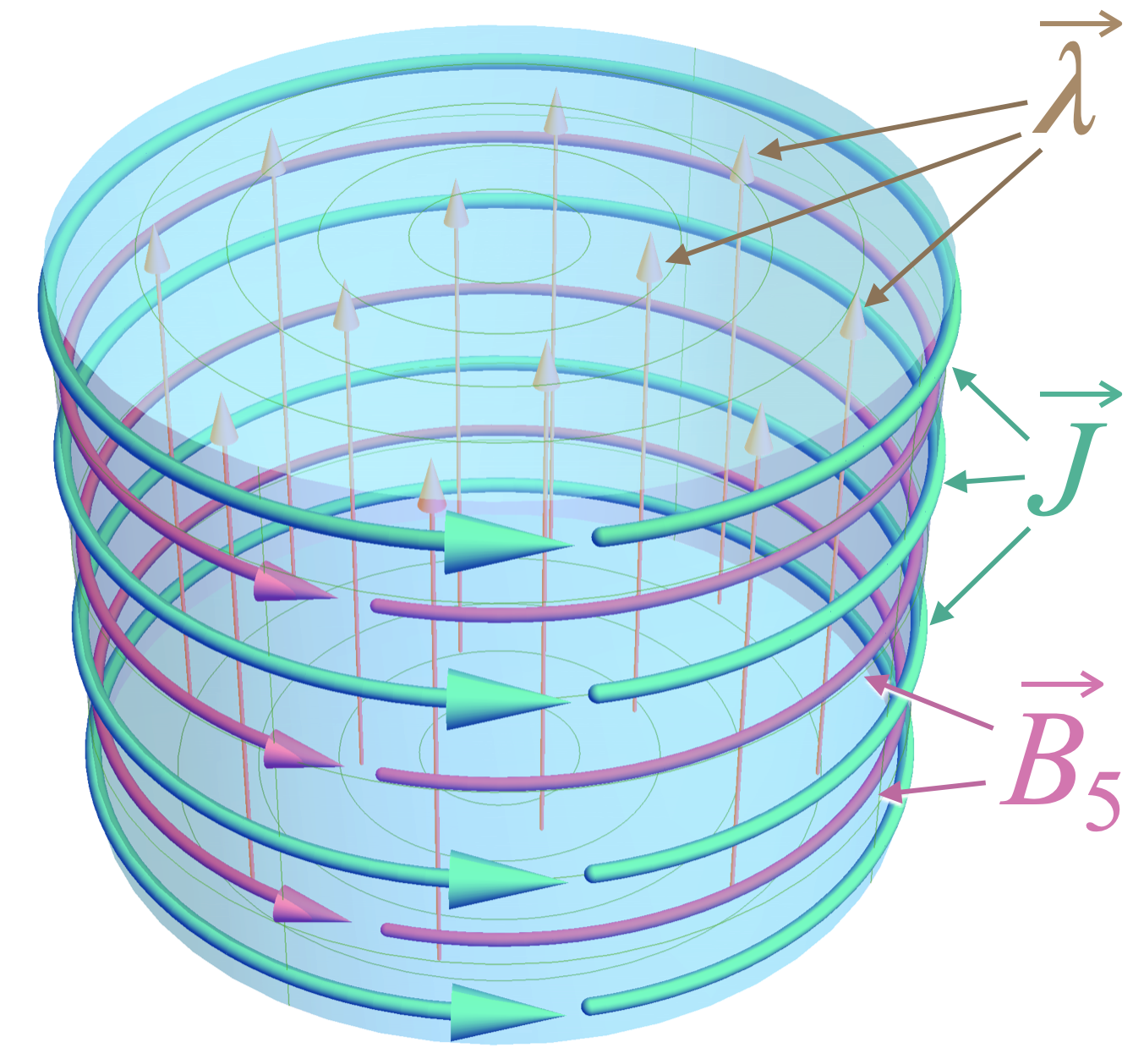
Figure 6: An AME energy current $\vec{J}$ (the light green arrows) around a cylinder of a Weyl semimetal induced by the axial gauge field ${\vec{B}}_{5}$ (purple arrows) generated due to the presence of a boundary as described in the text.

The axial magnetic effect is an anomaly induced transport phenomenon which consists on the generation of an energy current in the direction of an applied axial magnetic field ${\vec{B}}_{5}$:

$$T^{0i}=J^{i}_{\epsilon}=\sigma_{AME}B^{i}_{5}.$$ (167)

For a single (massless) Dirac fermion, i.e. one pair of Weyl-cones, the axial magnetic conductivity is

$$\sigma_{AME}=\frac{\mu^{2}+\mu^{2}_{5}}{4\pi^{2}}+\frac{T^{2}}{12}.$$ (168)

As discussed in Sec. V, the temperature dependent term in the axial magnetic effect (AME) conductivity coefficient comes from the gravitational contribution to the axial anomaly. Numerical evidence of the AME was reported in Braguta et al. (2013) but, since there are no axial magnetic fields in particle physics, this effect did not receive as much attention as the chiral magnetic effect.

The simplest example of a boundary pseudomagnetic field was proposed in the early work Chernodub et al. (2014). Consider a 3D cylinder of Weyl semimetal of height $L$ and basal radius $a$ as the one shown in Fig. 6 and choose the axis of the cylinder in the direction of the node’s separation, say OZ. Then, due to the boundary, the nodes separation will be

$$\vec{\lambda}=\hat{z}b_{z}\Theta(a-|r|).$$ (169)

We saw that the vector $\vec{\lambda}$ couples to the fermions as an axial gauge field. The corresponding axial magnetic field will point in the azimuthal direction as shown by the purple arrows in Fig. 6 and is proportional to the distance between the nodes:

$$B_{\theta}\sim\lambda_{z}\delta(|r|-a).$$ (170)

An energy current

$$J^{i}_{\epsilon}=\sigma_{AME}B^{i}_{5}$$ (171)

runs around the cylinder (green arrows in Fig. 6) with the coefficient given by eq. (168). This is an equilibrium current with zero divergence, another example of a magnetization energy current Shitade and Araki (2021).

In the original reference Chernodub et al. (2014), the temperature dependent of $\sigma_{AME}$ was used to propose a device which would be a direct evidence for the gravitational anomaly. In the setup of Fig. 6, the energy current would induce an angular momentum $L_{k}=\int_{\cal V}\varepsilon_{ijk}x_{i}T_{0j}$ along the axis of the cylinder (of volume ${\cal V}$):

$$L_{z}=\int_{\cal V}\varepsilon_{zr\theta}\;r\;J_{\epsilon}^{j}=2\pi\sigma_{AME}a^{2}\;L\lambda_{z}.$$ (172)

Plugging in the expression (168) for $\sigma_{AME}$ it follows that, at zero density and in the absence of a chiral imbalance the states at the edge of the cylinder posses an angular momentum of magnitude

$$L_{z}=\frac{N_{f}}{6}T^{2}\lambda_{z}{\cal V},$$ (173)

where $N_{f}$ is the total number of pairs of Weyl cones in the material. If the system, initially at a given temperature $T_{i}$, is heated to $T_{f}=T_{i}+\Delta T$ the angular momentum due to the AME will increase. Since the total angular momentum is conserved, the cylinder has to rotate in the opposite direction to compensate.

That the axial gauge fields would give rise to equilibrium magnetization currents was explicitly recognized in Grushin et al. (2016) were the Fermi arcs of Weyl semimetals were identified as the zeroth Landau level arising from the boundary pseudomagnetic field described here.

Other generalizations of anomalous transport phenomena due to axial gauge fields have been analyzed in the literature, see e.g. Refs Liu et al. (2017); Guan et al. (2017); Arjona et al. (2017); Gorbar et al. (2017c, d, e); Chernodub and Vozmediano (2019a); van der Wurff and Cortijo (2019); Liang and Ojanen (2019); Baggioli et al. (2020); Heidari and Asgari (2020); Gao et al. (2021). For an in-depth discussion of these issues we refer the reader to the focused reviews Ilan et al. (2020); Yu and Liu (2021). It is important to keep in mind that these fields must average to zero over a finite sample, which at times complicates their interpretation in lattice models Behrends et al. (2019).

VI.3 Curvature and elastic deformations

In the geometric formulation of elasticity, the strain tensor is identified with the metric of the slightly deformed flat space-time as:

$$g_{ij}=\delta_{ij}+\frac{1}{2}u_{ij}.$$ (174)

The identification of the underlying lattice supporting the electronic fluid with the external spacetime leads to the suggestion that we could induce gravitational anomaly effects with lattice deformations. In particular it would be tempting to try to induce curvature by deforming the lattice. The formalism of quantum field theory in curved space has a long history in the graphene literature González et al. (1992); Vozmediano et al. (2010) and, later, in Dirac and Weyl semimetals Cortijo and Zubkov (2016); Liang and Ojanen (2019). An important aspect of any realistc model for materials is that the induced metric in any dimension should have the structure

$$g_{\mu\nu}=\begin{pmatrix}1&0\\ 0&g_{ij}(x)\end{pmatrix},\quad$$ (175)

i.e., only the spacial part $g_{ij}(x)$ can be modified. This is a severe restriction on material realizations. Another important point to notice is that, while it is possible to induce curvature in a 2D sheet embedded in 3D by deforming the lattice in the third dimension, elastic deformations of a 3D lattice will always induce metrics with zero curvature Sun (2017).

Finally, notice that the elastic gauge fields defined in (163) are linear in the metric and would not appear in a covariant relativistic formulation. Linear terms can arise at finite temperature or chemical potential using the frame vector described in Appendix A. Being linear in the deformation, they are the most relevant terms for the physical implications.

VII The scale anomaly and thermoelectromagnetic currents

In this section we will analyze a set of new physical phenomena that arise in Dirac systems due to the scale anomaly, in both quantum field theory and in its material realizations. The scale or conformal anomaly Coleman (1985) is the breakdown of the scale invariance of a theory after its quantization. As we will see, in a perturbative sense the scale anomaly arises due to the emergence of a scale-dependence (“running”) acquired by the coupling constants of the theory in the process of renormalization.

A theory is said to be scale invariant when the classical equations of motion are invariant under a simultaneous rescaling of all coordinates and fields (denoted below as a generic field $\Phi$), according to their canonical dimensions $\Delta_{\Phi}$, with a global, coordinate-independent factor $\lambda$:

$$x^{\mu}\to\lambda^{-1}x^{\mu},\qquad\Phi(x)\to\lambda^{\Delta_{\Phi}}\Phi(x)\,.$$ (176)

One important example of a scale-invariant system is the low-energy behavior of gapless fermionic excitations in Dirac semimetals. As we mentioned in section II, a continuous symmetry of a classical system leads to the existence of a conserved Noether current. In particular, scale invariance implies the conservation of the dilatation current,

$$j_{D}^{\mu}=T^{\mu\nu}x_{\nu}\,.$$ (177)

The conservation of the current (177) at the level of the classical equations of motion,

$$\partial_{\mu}j_{D}^{\mu}=x_{\nu}\partial_{\mu}T^{\mu\nu}+T^{\mu}_{\nu}\delta_{\mu}^{\nu}=0\,,$$ (178)

together with the conservation of energy and momentum, $\partial_{\mu}T^{\mu\nu}=0$, implies the tracelessness of the energy-momentum tensor $T^{\mu\nu}$:

$$(T^{\mu}_{\mu})_{{\mathrm{cl}}}\equiv 0\,,$$ (179)

which is the signature of scale invariance in a physical system.

One should remark that the concepts “scale” and “conformal” (used with the words “transformation”, “invariance”, “anomaly”), are often employed interchangeably in the literature. Mathematically, these are different notions Nakayama (2015). In geometry, the scale transformation corresponds to an operation that modifies all spatial dimensions of an object by multiplying them with the same global scale factor (176). This global dilatation should be contrasted to the conformal transformation, constrained by a single requirement that after the conformal transformation, the angles between any intersecting curves or planes remain the same. Mathematically, the conformal transformation corresponds to a diffeomorphism, $x^{\mu}\to{x^{\mu}}{}^{\prime}=f^{\mu}(x)$, which leaves the metric unchanged up to an arbitrary multiplicative nowhere vanishing scalar factor $\Omega$:

$$g_{\mu\nu}(x)=\Omega^{2}(x^{\prime})g_{\alpha\beta}^{\prime}(x^{\prime})\frac{\partial{f^{\alpha}}}{\partial x^{\mu}}\frac{\partial{f^{\beta}}}{\partial x^{\mu}}\,.$$ (180)

A theory is said to be conformal in the classical sense when its action remains invariant under the conformal transformation (180) supplemented by an appropriate transformation of the fields according to their canonical dimensions. The conformal group has a bigger parameter space as compared to the single global dilatation parameter of the scale transformation.

Physically, the difference between the scale and conformal concepts is often ignored because all physically meaningful scale-invariant quantum field theories in three spatial dimensions exhibit conformal invariance, despite of the fact that the requirement of local conformal invariance is much stronger than the condition of global scale invariance Nakayama (2015). The renormalization group effects that will be discussed in this section break both the scale and conformal groups. To keep the mathematical rigor of Eq. (176), we will keep using the word “scale” in our review.

Other similar concepts that often appear in the literature are “Weyl invariance” (or “Weyl anomaly” if this invariance is anomalously broken) and “trace anomaly”. The first notion corresponds to the invariance of the action of the theory with respect to the rescaling of the metric by a local multiplicative factor, $\Omega>0$, along with the local scale transformation of the field:

$$g_{\mu\nu}(x)\to\Omega^{2}(x)g_{\mu\nu}(x)\,,\qquad\phi\to\Omega^{-\Delta_{\phi}}(x)\phi(x)\,.$$ (181)

As a local rescaling, the Weyl transformation (181) differs from the scale transformation (176), which is defined by a global rescaling of coordinates and fields, as well as from the conformal transformation (180), which is given by a diffeomorphism supplemented with a field transformation (which is not a rescaling, in general). As we mentioned above, physically meaningful theories do not distinguish between the scale and conformal notions Nakayama (2015) in a sense that both symmetries are either simultaneously broken or simultaneously respected. Weyl and conformal symmetries are also compatible in physical theories with certain exceptions in the form of exotic higher-derivative theories Karananas and Monin (2016) for which the conformal invariance does not automatically imply the invariance under Weyl transformations. All three (scale, conformal, and Weyl) symmetries are, however, broken by quantum fluctuations if the classically vanishing trace of the energy-momentum tensor (179) acquires a nonzero expectation value, $\left\langle T^{\mu}_{\mu}\right\rangle\neq 0$. Hence the name “trace anomaly”. All mentioned terms, “conformal anomaly”, “scale anomaly”, “trace anomaly”, or “Weyl anomaly”, are often used on equal footing in the literature with different names serving to stress slight but sometimes essential variations on the nature of the corresponding quantum effects.

VII.1 Scale anomaly in quantum electrodynamics

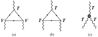
Figure 7: The three-point triangular (a) TVV and (b) TTT diagrams as well as the contact term (c) that generate the scale anomaly. The triangular diagrams involve the vector, $V^{\mu}=\gamma^{\mu}$, and graviton, $T^{\mu\nu}=i(\gamma^{\mu}\partial^{\nu}+\gamma^{\nu}\partial^{\mu})/2$, external lines.

As mentioned above, the scale invariance occurs in models with no dimensionful parameters: massless particles and dimensionless coupling constants. In the standard classification of renormalization, these couplings lead to strictly renormalizable models Zinn-Justin (2021). The scale anomaly is then associated to the running coupling constants of the model. In what follows we will describe this process in massless quantum electrodynamics, a paradigmatic model in quantum field theory which is also our main character for the condensed matter applications.

The Lagrangian of massless QED in a flat Minkowski space-time is

$${\mathcal{L}}=-\frac{1}{4}\left({\vec{B}}^{2}-\frac{1}{c^{2}}{\vec{E}}^{2}\right)+\bar{\psi}\Bigl{[}\gamma^{0}(i\partial_{t}-eA_{t})+{\vec{\gamma}}\cdot\Bigl{(}ic{\vec{\nabla}}-e{\vec{A}}\Bigr{)}\Bigr{]}\psi,$$ (182)

where $\psi$ is the Dirac four spinor, $\bar{\psi}=\psi^{\dagger}\gamma^{0}$ and $\gamma^{\mu}$ are the Dirac matrices. We have split the time and space components to show where the speed of light appears. In the condensed matter applications $c$ will be replaced by $v_{F}$. The electronic current is given by the variation of the action of the theory (182) $S=\int d^{4}x\,{\mathcal{L}}$ with respect to the electromagnetic field (39):

$$J^{\mu}=-\frac{\delta S}{\delta A_{\mu}}=e\bar{\psi}\Bigl{(}\gamma^{0},c{\vec{\gamma}}\Bigr{)}\psi.$$ (183)

For the purpose of this section, we restore the electric coupling $e$ in front of the electromagnetic gauge field $A^{\mu}$. The theory described by (182) is scale invariant at the classical level, which implies that the classical action (182) and, respectively, the classical equations of motion are invariant under a simultaneous rescaling of all coordinates and fields, according to their canonical dimensions (176)

$$x^{\mu}\to\lambda^{-1}x^{\mu},\qquad A_{\mu}(x)\to\lambda A_{\mu}(x),\qquad\psi(x)\to\lambda^{\frac{3}{2}}\psi(x).$$ (184)

It is convenient to write the Lagrangian (182) in the concise form

$${\mathcal{L}}=-\frac{1}{4}F^{\mu\nu}F_{\mu\nu}+{\bar{\psi}}i{\not{D}}\psi\,,$$ (185)

where ${\not{D}}=\gamma^{\mu}D_{\mu}$, with the covariant derivative $D_{\mu}=\partial_{\mu}-ieA_{\mu}$, and $F_{\mu\nu}=\partial_{\mu}A_{\nu}-\partial_{\nu}A_{\mu}$ is the field strength tensor of the gauge field $A_{\mu}$. Then the (symmetric) stress-energy tensor can be obtained by the variation of the action $S$ with respect to the background metric $g_{\mu\nu}$ (32),

$$T^{\mu\nu}(x) = -\frac{2}{\sqrt{-g}}\frac{\delta S}{\delta g_{\mu\nu}(x)}{\biggl{|}}_{g^{\mu\nu}=\eta^{\mu\nu}}=-F^{\mu\alpha}F^{\nu}_{\ \alpha}+\frac{1}{4}\eta^{\mu\nu}F_{\alpha\beta}F^{\alpha\beta}+\frac{i}{2}{\bar{\psi}}\left(\gamma^{\mu}D^{\nu}+\gamma^{\nu}D^{\mu}\right)\psi-\eta^{\mu\nu}{\bar{\psi}}i{\not{D}}\psi\,,$$ (186)

with $g=\det(g_{\mu\nu})$.

The tensor (186), is an identically traceless quantity in three spatial dimensions (179) (the fermionic part vanishes due to the classical equations of motion, ${\not{D}}\psi=0$).

In a generic interacting quantum field theory, quantum fluctuations break the classical scale invariance (184) due to the renormalization of the couplings of the model by quantum corrections. In quantum electrodynamics (182) the electromagnetic coupling $e$ “runs”, implying the emergence of a dependence of the electric coupling $e=e(E)$ on the energy scale $E$ of the interaction which involves a photon exchange Shifman (1991). This affects differently the physical phenomena that develop at different energy scales (or at different distances). This running of the coupling constant breaks the scale invariance in the quantum theory, and is a signature of the quantum scale anomaly.

The conformal anomaly reveals itself in a non-vanishing expectation value of the trace of the energy-momentum tensor (186). In the background of a classical electromagnetic field $A_{\mu}\equiv A^{\mathrm{cl}}_{\mu}$ one gets Shifman (1991)

$$\left\langle T^{\alpha}_{\ \alpha}(x)\right\rangle=\frac{\beta_{e}(e)}{2e}F^{\mu\nu}(x)F_{\mu\nu}(x),$$ (187)

where $\beta_{e}(e)$ is the beta-function associated with the running coupling $e$,

$$\beta_{e}=\frac{{\mathrm{d}}e(E)}{{\mathrm{d}}\ln E}\,,$$ (188)

normalized at the energy scale $E$. At the level of perturbation theory, the one-loop contribution to the scale anomaly (187) is generated by the TVV triangular Feynman diagram shown in Fig. 7(a). Despite its similarity with the anomalous vertices corresponding to the axial anomaly and the mixed axial-gravitational anomaly shown in Fig. 3, the scale anomaly is not one loop exact. This property is a natural consequence of the fact that any coupling of a generic quantum field theory acquires loop corrections at all orders of perturbation theory.

On the contrary, the pure curvature-dependent parts of the scale anomaly, discussed in Appendix C, are one-loop exact. They are generated by the three-point triangular, Fig. 7(b), and contact, Fig. 7(c), diagrams. The contact term is needed to maintain the general covariance of the anomalous contribution at the three-point level.

Physically, the appearance of the beta function (188) in quantum electrodynamics, is associated to the polarization of the vacuum by the creation and annihilation of short-living pairs of virtual particles and antiparticles due to quantum fluctuations. In matter it can be understood as associated to the screening of a test charge by the charges in the medium Fig. 8. This physical screening effect, reflected in non-vanishing beta function (188), is often associated with the “renormalization”: a mathematical procedure that is used to calculate the screening effect.

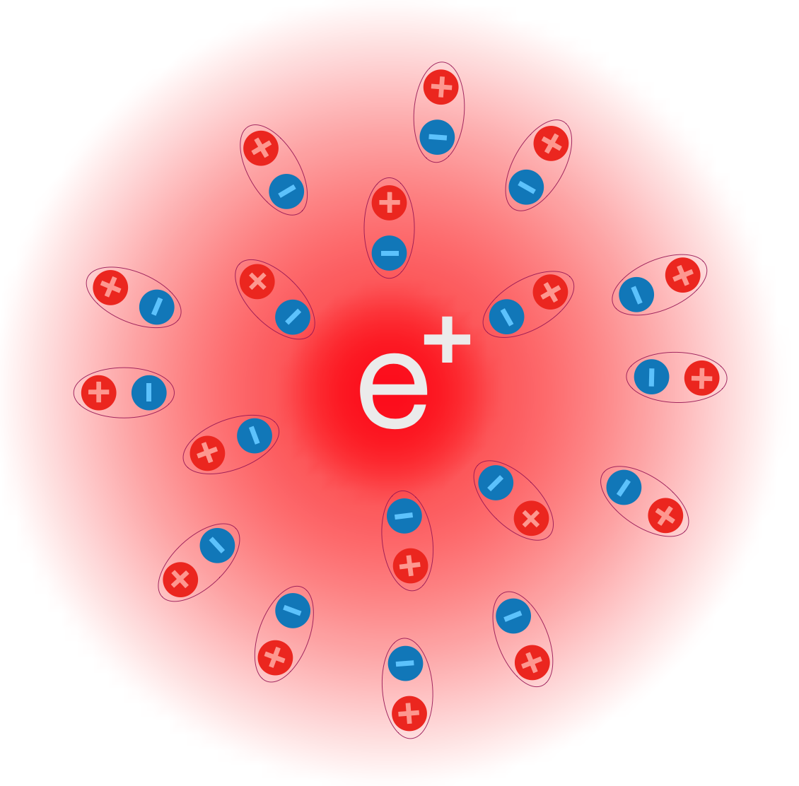
Figure 8: Screening of a test charge in quantum electrodynamics: the electric field of the test particle gets screened in the vacuum via polarization of the short-living particle-antiparticle pairs that are associated with tiny electric dipoles.

We would like to stress that the transport effects generated by the scale anomaly in an electromagnetic field background are exclusively associated to the running of the electric coupling $e$ with the energy scale. It is known that in the condensed matter systems, graphene being the paradigmatic example, the Fermi velocity is renormalized Gonzalez et al. (1994); Elias et al. (2011) and the scale anomaly is broken by the running of the Fermi velocity. But in the (2+1) version of QED describing graphene, the electric charge $e$ is not renormalized and the scale anomaly does not lead to any transport effects in response to the electromagnetic background fields. This is so even though the effective fine structure constant $\alpha\propto e^{2}/v_{F}$ runs with the energy in a very similar way as in QED Vozmediano (2011a, b). Since the running of the Fermi velocity is inessential for our purposes, in what follows, we consider a Lorentz-invariant formulation of the theory with $v_{F}=c$, which allows us to write formulas in a concise form. At the end of our discussion, we restore $v_{F}$ in the expressions.

The running of the coupling constant $e$ with the energy $E$ is governed by the renormalization group equation Peskin and Schroeder (1995):

$$E\frac{\partial e(E)}{\partial E}=-2b_{1}e^{3},$$ (189)

where the c-number parameter $b_{1}$ called also the bulk central charge of the model, is related to the beta function eq. (188) as $b_{1}=-\beta(e)/(2e^{3})$. In quantum electrodynamics with $N_{f}$ species of Dirac fermions, the one-loop beta function Eq. (188) is Peskin and Schroeder (1995):

$$\beta_{e}^{{\text{QED}}}(e)=N_{f}\frac{e^{3}}{12\pi^{2}}.$$ (190)

The renormalization group equation (189) allows to relate the value of the coupling constant at an energy $E$ with its value a a reference energy $E_{0}$ as

$$e^{2}(E)=\frac{e_{0}^{2}}{4b_{1}\ln\left(E/E_{0}\right)}.$$ (191)

VII.2 Scale anomaly and transport effects in the bulk

The scale anomaly (187) leads to anomalous transport effects which are easiest to analyze in a conformally flat space-time metric. A conformal transformation

$$g_{\mu\nu}(x)=e^{2\tau(x)}\eta_{\mu\nu}\,,$$ (192)

where $\tau(x)$ is a scalar conformal factor and $\eta_{\mu\nu}$ is the Minkowski metric tensor, induces, through the relation (187), the electric current:

$$J^{\mu}=-\frac{2\beta_{e}(e)}{e}\partial_{\nu}\left(F^{\mu\nu}\tau\right)\,,$$ (193)

where $e=\pm|e|$ is the elementary electron charge.

The current (194) is explicitly conserved: $\partial_{\mu}J^{\mu}=0$. For a classical electromagnetic field background, ($\partial_{\nu}\left(F^{\mu\nu}\tau\right)\equiv F^{\mu\nu}\partial_{\mu}\tau$) with $\partial_{\mu}\tau$ acting as a source of the gravitational perturbation, we get

$$J^{\mu}(x)=-\frac{2\beta_{e}(e)}{e}F^{\mu\nu}(x)\partial_{\nu}\tau(x)\,.$$ (194)

It is important to stress that, contrary to the transport phenomena generated by the axial and mixed axial-gravitational anomalies, the current (194) caused by the scale anomaly is produced by the quantum vacuum and emerges at zero chemical potential and zero temperature.

The expression (194) leads to two distinct transport effects which are realized in the presence of classical electromagnetic fields: The scale magnetic effect (SME) Chernodub (2016) refers to the generation of an electric current in a background magnetic field $\vec{B}$ and a weakly, conformally curved time-independent background, $|\tau|\ll 1$ :

$${\vec{J}}(x)=-\frac{2\beta_{e}(e)}{e}{\vec{B}}(x)\times{\vec{\nabla}}\tau(x)\,.$$ (195)

The electric current (195) is perpendicular to the magnetic field ${\vec{B}}$ and to the gradient of the gravitational perturbation, ${\vec{\nabla}}\tau$. This transport phenomenon is relevant for condensed matter applications as we discuss below.

In the presence of an electric background field ${\vec{E}}$ the conformal anomaly leads to the scale electric effect (SEE): An anomalous correction to the Ohmic contribution to the electric charge transport given by

$${\vec{J}}_{\mathrm{SEE}}=\sigma(x){\vec{E}}(x)\,,$$ (196)

where the metric-dependent anomalous electric conductivity is

$$\sigma(t,{\vec{x}}) = -\frac{2\beta_{e}(e)}{e}\frac{\partial\tau(t,{\vec{x}})}{\partial t}\,.$$ (197)

Since the conductivity (197) takes a nonvanishing value only in a time-dependent curved background, the condensed-matter applications of the SEE transport phenomenon are less transparent than these of its magnetic counterpart (195). We discuss the SEE transport phenomenon in Appendix C mentioning briefly its particle-physics applications relevant for the physics of the early universe.

VII.3 Anomalous thermoelectric current due to the conformal anomaly

The Nernst effect described in Section III, consists on the generation of an electric current perpendicular to a temperature gradient and to an applied magnetic field, Eq.  (18). The conductivity, Eq. (19) is determined by the components of the ${\bm{L}}^{(2)}$ transport tensor defined in Eq. (11). While the ordinary Nernst phenomenon appears due to thermal activation of the electron and hole charge carriers, we will see how the conformal anomaly can also generate the same effect with a coefficient proportional to the beta function of QED discussed in section VII.1.

For a metric with non vanishing $h^{00}$ component, the scale anomaly gives rise to the current (279)

$$\vec{J}=\frac{\beta(e)}{3e}\vec{B}\times\vec{\nabla}h^{00}.$$ (198)

Using the Luttinger relation $\vec{\nabla}T/T=-\vec{\nabla}\phi$ discussed in Sec. III.2, with $h^{00}=-2\phi$, and restoring the powers of the Fermi velocity $v_{F}$ (that replaces the velocity of light in the Dirac materials) and the value of the beta function, we get

$$\vec{J}=\frac{e^{2}v_{F}}{18\pi^{2}\hbar T}\vec{B}\times\vec{\nabla}T$$ (199)

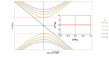
Figure 9: Landau level spectrum of a single chirality Weyl system. The inset represents the flat thermoelectric coefficient as a function of the chemical potential in the interval between the first Landau levels $n=\pm 1$ normalized to its value at $\mu=0$.

A standard Kubo calculation of the thermoelectric coefficient ${\bm{L}}^{(2)}$  (11) in the conformal limit ($T=\mu=0$) Arjona et al. (2019) also gave a non zero result numerically compatible with (199). Since the conformal anomaly is not exact, the numerical coefficient of the resulting transport phenomena has to be fixed by experiments.

Although the strict conformal situation (zero temperature and chemical potential) can not be realized in experimental conditions, there are measurable experimental signatures of the conformal anomaly induced transport. An additional computation of the thermoelectric coefficient as a function of the chemical potential done in Ref. Arjona et al. (2019) predicted a plateau at large magnetic fields which will remain at its $\mu=0$ value when $\mu$ lies in the interval between the first two Landau levels (see Fig. 9). The reason is that in the quantum limit only the zeroth Landau level is populated. The system is projected into the (1+1) conformal Landau level whose density of states is constant. Recent experiments in ZrTe₅, a Dirac semimetal Zhang et al. (2020), show this behavior from which we might extract the experimental value of the coefficient in eq. (199).

VII.4 Scale electromagnetic effects at the boundary

Another example of anomalous electric current generation appears near a reflective boundary of a homogeneous system. While this transport effect is not directly related to the thermal transport, the presence of the boundaries allows us to get an insight into the physics of the renormalization, which plays a role in the thermomagnetic effects produced by the scale anomaly.

We consider a boundary that reflects the quasiparticles but is completely transparent to photons. Our motivation is that this boundary conditions give a simple model of a material in which the electrons are confined to the inside but the photons can escape to the space outside the material. We also emphasize that our considerations apply at the charge neutrality point in which the density of classical charge carriers vanishes. This implies that no classical screening can take place.

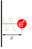
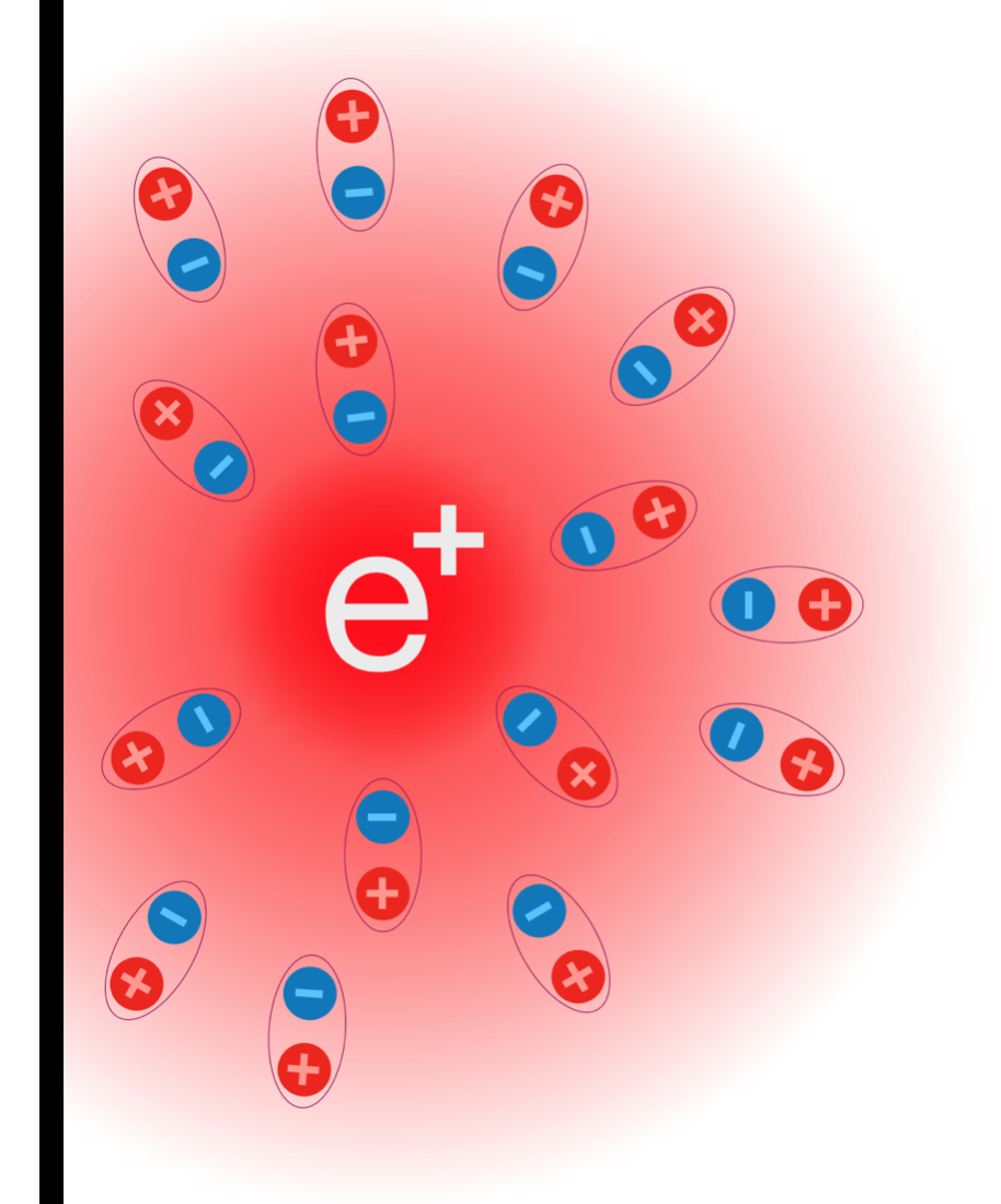
(a)	(b)

Figure 10: (a) Particle near the reflective non-conducting boundary. (b) Effect of the boundary on charge screening.

An intuitive explanation of the influence of the boundary on the renormalization of electric charge appears from the consideration of the screening in real space. We know already that the charge screening is due to the polarization of the medium or vacuum by the electric field of the test particle, Fig. 8. The polarization effect, however, decreases when the test particle approaches the boundary at a distance smaller than the polarization distance. Due to a purely geometrical effect, schematically shown in Fig. 10, part of the polarizing pairs disappear and the screening of the test charge becomes less effective. When the particle approaches the boundary too close, the screening is incomplete due to geometrical reasons. The renormalization of the electric charge then becomes sensitive to the distance to the boundary of the system $x_{\perp}$. We can translate the distance to the boundary to a momentum scale $p_{\perp}=\frac{\hbar v_{f}}{x_{\perp}}$. This sets the scale of the renormalized charge $e=e(p_{\perp})$ implying the aforementioned dependence on the distance $x_{\perp}$.

Having qualitatively established that the presence of an edge affects the renormalization of the electric charge near the edge, we can wonder if the electromagnetic fields produce any electric transport effect close the boundary. The answer to this question was given by McAvity and Osborn about thirty years ago. In Ref. McAvity and Osborn (1991) these authors showed that a classical electromagnetic field acting on a bounded quantum system of charged particles, generates an electric current $J^{\mu}$ in the vicinity of the flat boundary. In a Lorentz invariant theory with $v_{F}=c$, the expression of the current has the form Chu and Miao (2018a, b):

$$J^{\mu}(x)=-\frac{2c\beta_{e}}{e\hbar}\frac{F^{\mu\nu}(x)n_{\nu}}{x}\,,$$ (200)

where $n^{\mu}=(0,{\vec{n}})$ is the inside pointing normal vector to the edge of the system, and $x>0$ is the spatial distance from the point where the current (200) is measured to the boundary along the spatial vector ${\vec{n}}$. The prefactor in Eq. (200) is given precisely by the beta function (188) which implies that the boundary effect (200) is generated by the scale anomaly. While we have given an intuitive interpretation of this effect with partially transparent boundary conditions it turns out that the current is universal in the sense that it actually does not depend on the particular choice of boundary conditions McAvity and Osborn (1991); Chu and Miao (2018a, b).

Notice the striking similarity between the coefficients in the edge electric current (200) and the bulk electric current induced by the scale electromagnetic effect (194). Both are proportional to the beta function and both appear at zero temperature and chemical potential.

In order to explore the possible consequences of the previous result on a physical system, in particular on a Dirac metal, it is convenient to rewrite the edge electric current (200) in the reference frame of the crystal:

$${\vec{J}}=-\frac{2v_{F}\beta_{e}}{e\hbar}\frac{1}{x}{\vec{n}}\times{\vec{B}}\,,$$ (201)

where we have also replaced the speed of light $c$ with the Fermi velocity $v_{F}$. The current is normal to the axis of the magnetic field and tangential to the boundary of the system. This scale magnetic effect at the edge (SMEE) is the direct analogue of the SME phenomenon (195) which takes place in the bulk.

The existence of the “scale magnetic edge effect” (201) was recently demonstrated in first-principles numerical simulations of scalar quantum electrodynamics with one species of massless scalar field Chernodub et al. (2019).

The anomalous edge current (201) can be interpreted in an analogous way to the edge currents that appear in the description of the classical Hall effect. In the Hall effect, an electron moves along the boundary in the form of skipping orbits which represent circular segments joined together at the reflecting events at the boundary of the system. Contrary to the classical Hall effect, the anomalous current (201) emerges in the vacuum where the chemical potential is zero. The vacuum edge current appears as a result of skipping orbits of the virtual particles and antiparticles created by the quantum fluctuations near the edge of the system in the background magnetic field Chu and Miao (2018a, b). In the condensed matter context, the notion of vacuum corresponds to exact neutrality point where the sharp, zero-temperature Fermi level goes precisely through the Dirac point. Contrary to the helical edge currents that appear in quantum spin-Hall systems Wu et al. (2006) and the chiral edge states in Chern insulators Haldane (1988), the current (201) generated by the scale anomaly does not form an exponentially thin boundary layer.

We also emphasize that the edge current (201) is a magnetization current which affects the magnetic moment of the system but does not lead to a net transport of electric charge.

The temporal component of the edge four-current (200) leads to the accumulation of electric charge at the edge of the system in the presence of a static electric field ${\vec{E}}$:

$$\rho=-\frac{2v_{F}\beta_{e}}{e\hbar c^{2}}\frac{{\vec{n}}\cdot{\vec{E}}}{x}.$$ (202)

This is the “scale electric edge effect” (SEEE). It can also be viewed as an analogue of the scale electric effect (SEE) in the bulk (196). While the bulk SEE phenomenon does not have so far any visible potential for the experimental verification in the condensed matter context, its edge counterpart (202) has a direct implication for the electrostatic charge screening in semimetals at the charge neutrality point as we will explain now.

An ideal conductor totally screens the electrostatic field in its bulk due to the presence of mobile charge carriers. The carriers redistribute themselves under the influence of an external electric field in such a way as to precisely compensate the external field  Ashcroft et al. (1976).

In ordinary conductors, the static electric field falls down with an exponential law close to the boundary,

$$\frac{E(x)}{E(0)}\propto e^{-x/\lambda}\,,$$ (203)

where the screening length $\lambda$ determines the width of the boundary layer of the redistributed mobile carriers. In usual metals, this width coincides with the Thomas-Fermi wavevector, which is a very small quantity in the typical range of a few nanometers. However, in the scale-invariant limit of vanishing density and temperature, all the parameters of the system reduce to dimensionless quantities and the Fermi liquid phenomenology can no more be used. In particular, the screening length $\lambda$ becomes infinite and the standard picture of the electrostatic charge screening is invalid.

However, even in the conformal limit of the exact zero-temperature neutrality point of a Dirac semimetal the electrostatic field gets screened Chernodub and Vozmediano (2019b). Remarkably, the screening occurs via the scale anomaly. The background electric field polarizes the bulk of the system and generates, via the SEEE (202), a wide boundary layer of the redistributed mobile carriers. The accumulated boundary charge screens the background electric field in the form of a power law,

$$\frac{E(x)}{E(0)}\propto x^{-\nu}\,,$$ (204)

rather then the exponential (203). The conformal (or scale) screening exponent,

$$\nu=\frac{2\beta_{e}}{ec\hbar\varepsilon_{0}}=\frac{e^{2}}{6\pi^{2}\hbar v_{F}\varepsilon\varepsilon_{0}},$$ (205)

is determined by the beta function related to the renormalization of the electric charge (188). The last relation for the conformal exponent in Eq. (205) is given for a single cone of the Dirac semimetal with the bulk permittivity $\varepsilon$. In typical semimetals, the conformal exponent is predicted to be rather large, $\nu\sim 0.1$, which makes its experimental detection feasible via the measurement of the electrostatic charge accumulation or the electrostatic potential along the sample Chernodub and Vozmediano (2019b).

VIII Torsion and chiral transport

Torsion is a geometric property of space-time. In the theory of general relativity, space-time is assumed to be torsionless, and its geometry is entirely defined by curvature. This is so because there is seemingly no experimental evidence of torsion in the space-time of our universe. However, there are extensions of general relativity that include torsion, like Einstein-Cartan theory Hehl et al. (1976). Perhaps surprisingly, such theories have acquired special relevance in a completely different area of physics: the geometric description of point defects in crystals Nelson (2002) and the coupling of the electrons to the lattice degrees of freedom.

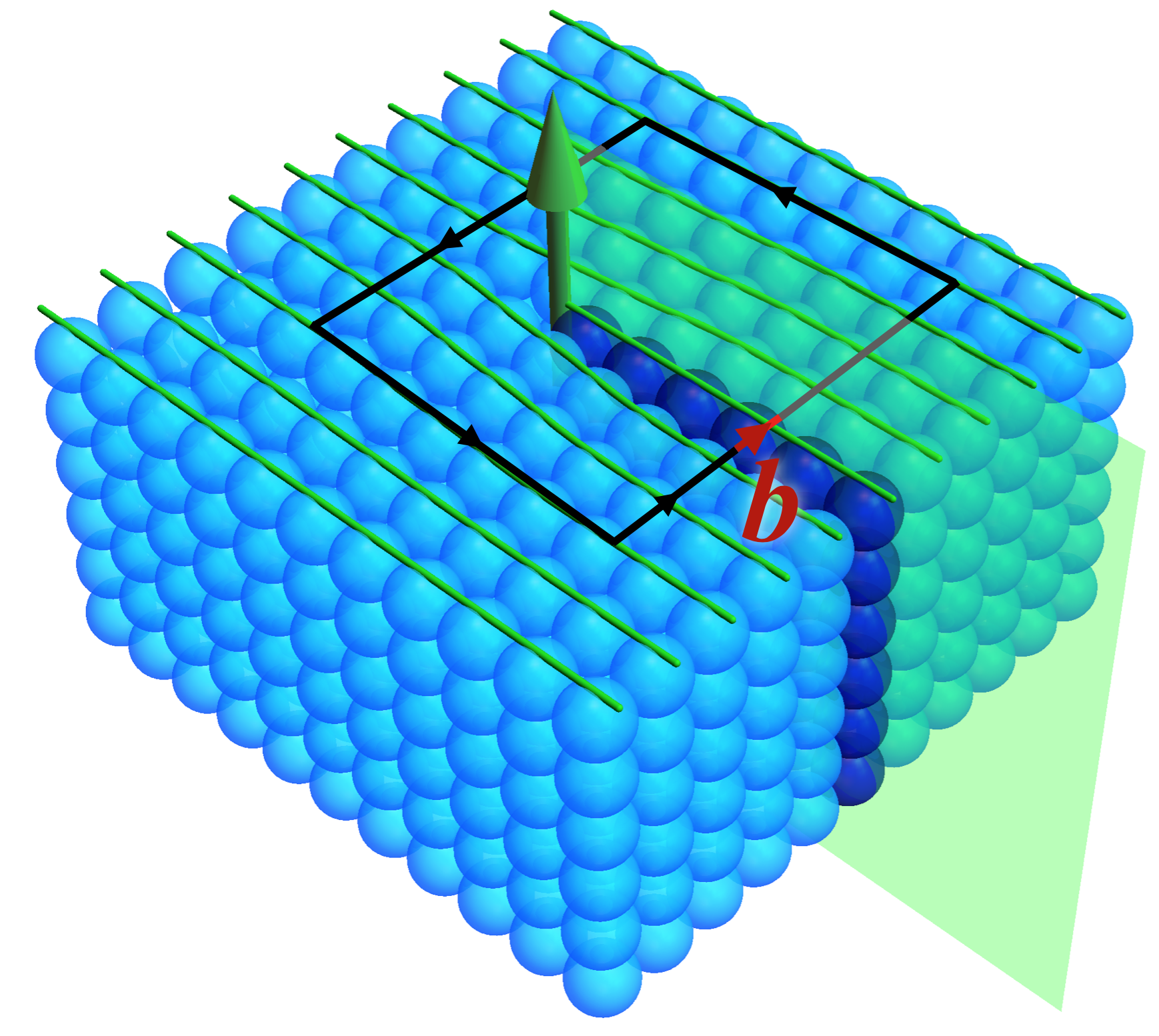
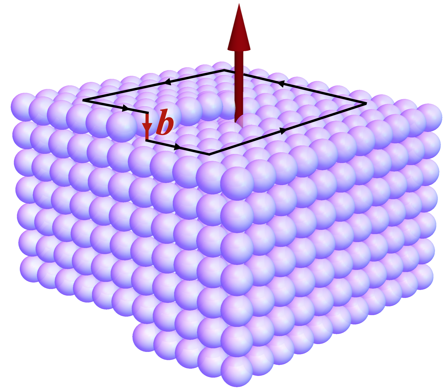
(a)	(b)

Figure 11: (a) Edge dislocation in a square lattice. Closed loops around the dislocation result in a translation along the dislocation line. The Burgers vector is perpendicular to the dislocation plane. (b) Screw dislocation. The Burgers vector is parallel to the dislocation line.

Torsion appears naturally associated to dislocations Katanaev and Volovich (1992); Kleinert (1989), line defects that play a very important role in the plastic deformation in crystals. They are classified in two types. The first type are edge dislocations, shown in Fig. 11(a), which can be visualized as the addition of an extra half plane of atoms midway through the crystal. As a consequence, discrete closed paths encircling the dislocation line in the lattice do not close. The vector joining the end with the starting point is called Burgers vector ${\vec{b}}$ which in this case is perpendicular to the dislocation line. The second type are screw dislocations, which are more difficult to visualize. A schematic one is shown in Fig. 11(b). Again discrete closed paths do not close and the Burgers vector in this case is parallel to the dislocation line. The failure to close of discrete paths can also be seen as the non-commuting of parallel displacements paths going from A to B in different directions of the lattice. This operation, for the parallel transport of a vector, is given by the commutator of two covariant derivatives acting on the vector. The result, going back to the formalism of curved spaces in the continuum (see appendix B) is

$$[\nabla_{\mu},\nabla_{\nu}]V^{\rho}=R\,^{\rho}\,_{\sigma\mu\nu}V^{\sigma}+\theta^{\sigma}_{\mu\nu}\nabla_{\sigma}V^{\rho}.$$ (206)

While curvature gives a rotation of the vector, torsion (represented by the torsion tensor $\theta^{\sigma}_{\mu\nu}$) results in the non-closure of the four successive translations by an extra translation. In a more compact wording, torsion describes the failure of a parallelogram spanned by two vectors to form a closed curve.

Since the emergence of materials with relativistic quasiparticles, like Dirac and Weyl semimetals, establishing a consistent treatment of the coupling of torsion to relativistic fermions, with the associated possible influence of torsion in the electric responses, has become an important task in the context of condensed matter de Juan et al. (2010); Hughes et al. (2013); Parrikar et al. (2014); Ferreiros et al. (2019); Huang et al. (2019, 2020a); Nissinen and Volovik (2019, 2020); Nissinen (2020); Huang and Han (2020); Laurila and Nissinen (2020); Huang et al. (2020b); Liang and Ojanen (2020); Khaidukov and Zubkov (2018); Imaki and Yamamoto (2019); Imaki and Qiu (2020). Moreover the coupling of electronic excitations to the new geometric objects could potentially induce additional anomalous terms in the effective action which may give rise to novel anomaly–induced transport phenomena. In what follows we will give a different perspective on torsional anomalies as compared to some of the works in the literature, and address the presence (or more precisely absence) of chiral responses to torsion.

VIII.1 Nieh-Yan current

Recently, there has been an increasing interest in condensed matter in what has been called torsional (or Nieh-Yan) anomaly Obukhov (1982); Nieh and Yan (1982); Obukhov (1983); Yajima (1988, 1996); Chandía and Zanelli (1997); Parrikar et al. (2014); Hughes et al. (2013); Ferreiros et al. (2019); Huang et al. (2019, 2020a); Nissinen and Volovik (2019, 2020); Nissinen (2020); Huang and Han (2020); Laurila and Nissinen (2020); Huang et al. (2020b). The conservation equation (or Ward identity) for the axial current in the presence of torsion ($\theta^{\sigma}_{\mu\nu}$) reads

$$\nabla_{\mu}J^{\mu}_{5}-\theta^{\lambda}_{\lambda\mu}J^{\mu}_{5}=\mathcal{A}^{g}_{5},$$ (207)

where the functional $\mathcal{A}^{g}_{5}$ accounts for the presence of gauge anomalies. It has been argued that $\mathcal{A}^{g}_{5}$ receives a torsion contribution, beyond the axial and mixed axial-gravitational anomalies, given by the so called Nieh-Yan term Nieh and Yang (2007), resulting in

$$\nabla_{\mu}J^{\mu}_{5}-\theta^{\lambda}_{\lambda\mu}J^{\mu}_{5}=c_{T}\epsilon^{\mu\nu\rho\lambda}(\eta_{ab}\theta^{a}_{\mu\nu}\theta^{b}_{\rho\lambda}-R_{ab\mu\nu}e^{a}_{\rho}e^{b}_{\lambda}).$$ (208)

For the right-hand side of Eq. (208), the Nieh-Yan term, to have the correct dimension, the coefficient $c_{T}$ must have dimensions of inverse square length $c_{T}\sim l^{-2}$. In vacuum, the only candidate scale is the cut-off $\Lambda$, so that the value of $c_{T}$ must depend on regularization. This means that the contribution in Eq. (208) can be removed by a suitable local term in the background fields, usually called counterterm in the language of quantum field theory.

That the Nieh-Yan term can be removed is further reinforced by noticing that it can be written as a total derivative of well defined fields $e^{a}_{\mu}$ and $\theta^{a}_{\mu\nu}$: $\nabla_{\mu}(\epsilon^{\mu\nu\rho\lambda}\eta_{ab}e^{a}_{\nu}\theta^{b}_{\rho\lambda})$. The vielbein and torsion tensor are covariant objects under diffeomorphisms and local Lorentz rotations, see Appendix B, and thus the product inside the derivative is well defined. This is unlike the second Chern class $\epsilon^{\mu\nu\rho\lambda}F_{\mu\nu}F_{\rho\lambda}$ or the Pontryagin class $\epsilon^{\mu\nu\rho\lambda}R^{a}_{\,b\,\mu\nu}R^{b}_{\,a\,\rho\lambda}$, which determine the chiral and axial-gravitational anomalies, respectively. The latter two cannot be written as derivatives of well defined tensors. Rather, the corresponding Chern-Simons terms explicitly depend on the local value of $A_{\mu}$ or $\omega_{\mu}\,^{a}\,{}_{b}$, which are not tensors but transform as connections. Being a total derivative of well defined fields, the Nieh-Yan contribution to the non-conservation of the axial current in Eq. (208) must therefore come from a local term in the effective action of the form

$$S_{eff}^{NY}=c_{T}\int d^{4}x\,e\,\epsilon^{\mu\nu\rho\lambda}\eta_{ab}A^{5}_{\mu}e^{a}_{\nu}\theta^{b}_{\rho\lambda}.$$ (209)

The above arguments show that the torsional ”anomaly” is not an anomaly in the formal quantum field theory sense, since the corresponding Nieh-Yan term can be removed by choosing a suitably regularization. It is more precise to understand it as a local, regularization dependent, torsion contribution to the axial current

$$J_{5}^{\mu}=c_{T}\epsilon^{\mu\nu\rho\lambda}\eta_{ab}e^{a}_{\nu}\theta^{b}_{\rho\lambda}.$$ (210)

This still leaves the problem of the cut-off scale ($\Lambda$) dependence of the coefficient $c_{T}$, which therefore seems highly ambiguous from the standpoint of relativistic quantum field theory. However in a condensed matter context in which there is a natural cutoff, such currents could appear, as it has been first argued in Hughes et al. (2013); Parrikar et al. (2014). This argument has been subsequently exploited in Ferreiros et al. (2019); Huang et al. (2019, 2020a); Nissinen and Volovik (2019, 2020); Nissinen (2020); Huang and Han (2020); Laurila and Nissinen (2020); Huang et al. (2020b), where the Nieh-Yan term has been discussed in the context of Dirac/Weyl semimetals and superfluids.

VIII.2 Absence of universal chiral torsional transport

We have discussed in depth how the chiral anomaly is responsible for chiral universal transport, in the form of the CME and CVE, as a response to magnetic and vorticity fields. A pertinent question then is wether there exists such kind of chiral transport as a response to geometric torsion. We have argued that the possible existence of an additional Nieh-Yan contribution to the conservation equation of the axial current, is better understood directly as a torsional response in the current (Eq. (210)). The coefficient $c_{T}$ of such a response must have units of inverse squared length, and therefore must depend on regularization through the only such possible scale in vacuum, the cut-off. However, the presence of matter could source two additional IR scales, temperature and chemical potential, that could do the trick. It has been argued that, in fact, finite temperature effects could provide a universal coefficient $c_{T}\propto T^{2}$ Huang et al. (2020a); Nissinen and Volovik (2019, 2020); Liang and Ojanen (2020).

One can attempt to do a systematic study, as has exactly been done recently in Ferreiros and Landsteiner (2020), and write down all possible dissipationless chiral transport terms, as a response to the torsion tensor (to linear order), derive the corresponding Kubo formulas, and compute them. This basically searches for parity even coefficients, analogues of the CME and CVE for torsion. To do this, we follow appendix A and take into account that an equilibrium state of a quantum statistical system is defined not only by the temperature and the chemical potential for the electric charge, but also by the chemical potentials for the rest of conserved charges. Therefore the state is characterized by $T$, $\mu$, and the four components of the velocity $u^{a}$, which are the chemical potentials for the momenta. $u^{a}$ is a normalized four velocity, $u_{a}u^{a}=1$, so only three components are independent corresponding to the three momenta. The approach in Ferreiros and Landsteiner (2020) was to write down all possible parity even terms in the (axial) current at lowest order in torsion and vorticity $\Omega^{\mu}=\frac{1}{2}\epsilon^{\mu\nu\rho\lambda}u_{\nu}\partial_{\rho}u_{\lambda}$, with $u_{\mu}=u_{a}e^{a}_{\mu}$

$$J^{\mu}_{(5)}=\rho_{(5)}u^{\mu}+\sigma^{\Omega}_{(5)}\Omega^{\mu}+\epsilon^{\mu\nu\rho\lambda}\Big{(}\frac{c_{T,(5)}^{||}}{2}P^{||}_{ab}e^{a}_{\mu}\theta^{b}_{\nu\rho}+\frac{c_{T,(5)}^{\perp}}{2}P^{\perp}_{ab}e^{a}_{\mu}\theta^{b}_{\nu\rho}\Big{)}.$$ (211)

$P^{\parallel}_{ab}=u_{a}u_{b}$ and $P^{\perp}_{ab}=\eta_{ab}-u_{a}u_{b}$ are the projectors parallel and orthogonal to the velocity field, and $\rho_{(5)}$ is the (axial) charge density. The second term is the CVE, and the two last terms represent the response to torsion. In Ferreiros and Landsteiner (2020) it was found that

$$c_{T,(5)}^{||}=c_{T,(5)}^{\perp}=0.$$ (212)

This result means that there is no analogue of the CME and CVE for torsion. In other words, there are no universal chiral torsional responses (at least at lowest order), which may be related to the fact that there is no torsional quantum field theory anomaly as discussed earlier, and as such no anomaly related torsion transport coefficients. This might seem at odds with some recent works Khaidukov and Zubkov (2018); Imaki and Yamamoto (2019); Imaki and Qiu (2020), but the apparent contradiction is solved by realizing that those results can be understood just as a response to vorticity in a general background, through the CVE

$$J^{\mu}_{(5)}=\sigma^{\Omega}_{(5)}\Omega^{\mu}=\frac{\sigma^{\Omega}_{(5)}}{2}\epsilon^{\mu\nu\rho\lambda}u_{a}u_{b}e^{a}_{\nu}\partial_{\rho}e^{b}_{\lambda},$$ (213)

with $u^{a}=(1,0,0,0)$ in the rest frame of the fluid. By taking small perturbations around flat space-time $e^{a}_{\mu}=\delta^{a}_{\mu}+h^{a}_{\mu}$, the vorticity can be written in terms of the gravitomagnetic field (see Appendix D) $2\vec{\Omega}=\vec{B}_{g}=\vec{\nabla}\times\vec{A}^{g}$, with $A^{g}_{i}=h^{t}_{i}$, and the CVE can be non-zero even if the fluid is at rest

$$\vec{J}_{(5)}=\sigma^{\Omega}_{(5)}\vec{\Omega}=\frac{\sigma^{\Omega}_{(5)}}{2}\vec{\nabla}\times\vec{A}^{g}.$$ (214)

Note that there is no torsion here. One should not confuse the gravitomagnetic field, arising as a consequence of having vorticity in a general curved background, with the torsion tensor.

IX Experimental advances

Throughout this review we have gathered how different conductivity tensors have contributions from various anomalies. Several groups have attempted to measure these contributions experimentally in condensed matter systems that host Weyl semimetals Armitage et al. (2018).

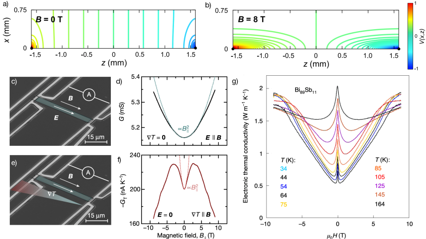
Figure 12: a) and b) show calculated equipotential lines in the presence and absence of a magnetic field, respectively. The bending of equipotential lines results in a spurious measurement of intrinsic magneto-conductance known as current jetting (adapted from Arnold et al. (2016)). c) Experimental setup to measure the chiral anomaly enhanced magnetotransport in NbP (adapted from Gooth et al. (2017)). d) The magneto-conductivity is quadratic with field at low magnetic fields and linear at high magnetic fields. e) Experimental setup to measure the mixed-axial gravitational anomaly enhanced magneto-thermal transport in NbP (adapted from Gooth et al. (2017))). f) The anomalous contribution to magneto-thermal conductivity is quadratic with field at low magnetic fields and vanishes at high magnetic fields (adapted from Gooth et al. (2017)). g) Anomalous electronic contribution to the thermal conductivity measured in Ref. Vu et al. (2021).

In magneto-electric transport it is the longitudinal conductivity that is enhanced by the chiral anomaly Son and Spivak (2013). This phenomenon is referred to as a positive magneto-conductance or, equivalently, a negative magnetoresistance due to the chiral anomaly. The anomalous contribution to conductance in lattice models can be traced back to work by Nielsen and Ninomiya Nielsen and Ninomiya (1983b), which considered a collinear electric and magnetic field, activating the chiral anomaly. Through our arguments in (4), the effect of these is to pump right movers into left movers (or vice versa), creating a chiral chemical potential $\mu_{5}$, which then drives a current through the chiral magnetic effect (90). At small magnetic fields this results in a $B^{2}$ dependence of the magneto-conductivity, as dictated by (142), while at high magnetic fields the dependence on $B$ is linear, as dictated by (160).

Numerous theoretical and experimental works have observed negative magnetoresistence consistent with that predicted by the chiral anomaly Armitage et al. (2018). In some materials, typically with low mobility, the intrinsic contribution can be isolated Ong and Liang (2021). However, spurious effects complicate the interpretation of an enhanced conductivity based solely on the chiral anomaly. Among them, current jetting is specifically problematic (see Figs. 12a) and b)). Current jetting occurs when electrons enter a material with an anisotropic electrical conductivity $\sigma$ and high mobilities through a point contact, bending the otherwise equidistant equipotential lines Arnold et al. (2016); Reis et al. (2016); Ong and Liang (2021). Because of this bending, the voltage drop in the sample becomes inhomogeneous, and the value measured becomes sensitive on where the contacts are placed. If sizable, current jetting can jeopardize measuring intrinsic effects, such as the anomalous enhancement of transport. Current jetting is enhanced in a magnetic field because it increases the anisotropies between the different components of the conductivity tensor, especially in high mobility samples. While the strength of this effect can be tested Ong and Liang (2021), and experimental precautions can be taken against this detrimental effect, e.g. choosing materials with reduced carrier mobility, it severely reduces the pool of materials to test anomalous behaviour.

In Sec. (4) we saw how anomalous transport enhancement can occur also in the longitudinal magneto-thermal, and magneto-thermoelectric transport due to the mixed axial-gravitational anomaly (see (142) and (160)) Landsteiner et al. (2011a). The first experimental observation of the enhancement of magneto-thermoelectric transport in a Weyl semimetal was reported by Gooth et al in NbP samples Gooth et al. (2017). These samples displayed a longitudinal magneto-conductance ($\sigma_{ii}(B)$) that increased with magnetic field $B$, which was maximal when $B$ was parallel to the applied electric field. They observed that $\sigma_{ii}(B)\propto B^{2}$ at low magnetic fields and $\sigma_{ii}(B)\propto|B|$ at high-magnetic fields, in accordance to what is expected from the chiral anomaly (see (142) and (160) and Figs. 12(c) and (d)). Additionally, they observed that the longitudinal magneto-thermoelectric conductance increased as $B^{2}$ at low magnetic fields, and was then suppressed at high fields, again consistent with (142) and (160) (see Figs. 12e) and f)). These observations, together with the fact that the longitudinal magnetothermal conductance was maximal when $B$ was parallel to the applied thermal gradient, motivated the authors to conclude that their observations were consistent with the signatures of the mixed-axial gravitational anomaly (see section 4).

The mixed-axial gravitational anomaly also predicts the enhancement of the longitudinal magneto-thermal conductivity $\kappa_{ii}(B)$ through (142) and (160). Such an enhancement is consistent with observations in GdPtBi Schindler et al. (2020) and a Weyl state induced in the alloy Bi_1-xSb_x Vu et al. (2021) (see Fig. 12g)). The benefit of measuring $\kappa_{ii}(B)$ as a probe of anomalous thermal transport is that it does not suffer from the extrinsic effect known as current jetting. The reason is that this measurement does not involve electrical contacts. The electronic thermal transport is achieved through thermalization of thermal contacts mainly by scattering with phonons, which does not occur at a point contact. The measurement of $\kappa_{ii}$ also has the benefit of circumventing other effects, like contact misalignment Vu et al. (2021).

The magnetic field dependence of the different transport coefficients can be derived semiclassically Lundgren et al. (2014) without an explicit connection to anomalies. However, Kim and Stone observed in Stone and Kim (2018) that the derivations that do take into account the dependence on the different anomalous coefficients ($b_{a}$ and $d_{abc}$, see (80)) explicitly offer a chance to understand the physical origin of these anomalies. These authors proposed a physical picture that explicitly connected the gravitational anomaly to heat flow and provided some physical intuition, which we discussed briefly in V.2 and in detail in Appendix E.

X Conclusions

The seminal work of Luttinger Luttinger (1964) established a deep relation between geometry and thermal transport phenomena of condensed matter systems near equilibrium. While this relation allows to understand how Kubo formulas for thermal transport can be derived it is a classical relation at its heart. On the other hand many realms of modern condensed matter physics have to deal with intrinsically quantum mechanical aspects of the collective behaviour of electronic quasiparticles in crystals. This is especially apparent in the field of Weyl and Dirac matter in which the intrinsically quantum mechanical properties play a decisive role. This has lead to the extraordinarily interesting situation that concepts originally home to high energy physics such as anomalies of quantum field theories are nowadays at the center of research in condensed matter physics. In view of this development it is necessary to uplift Luttinger’s original ideas into this new quantum era of condensed matter physics. In this review we collected the basic ideas behind Luttinger’s original approach but we also have reviewed some of its substantial generalizations relevant this new quantum era. In particular we highlighted the role played by various anomalies in the theory of transport phenomena and its application to Weyl and Dirac matter.

An intriguing aspect of anomaly induced transport is that at first it seems unrelated to the formalism put forward by Luttinger. Both the dependencies of the conductivities (92)-(95) temperature and chemical potential can be derived from a microscopic perspective without any reference to anomalies. They simply arise from the standard Sommerfeld integrals involving the Fermi-Dirac distribution. However, as first noticed in Landsteiner et al. (2011a) the general formulas immediately reveal this relations because they are directly proportional to the anomaly coefficients $d_{abc}$ and $b_{a}$. The approach in Ref. Stone and Kim (2018) relies on a rather interesting marriage of Luttinger’s ideas with Hawking’s ideas on thermal radiation of black holes. While the original Luttinger formalism is based on classical ideas about gravity it seems in hindsight appropriate that quantum transport, such as the chiral magnetic and chiral vortical effects, calls for the inclusion of ideas from the realm of quantum gravity as is Hawking radiation. The so far anecdotal similarity between the Sommerfeld integrals that determine quantum transport and the anomaly generating functional highlighted in Ref. Loganayagam and Surowka (2012); Stone and Kim (2018) act as a motivation to develop further the link between chiral anomalies and thermal transport. Another aspect is the role played by the discrete (or global) anomaly pointed out in Golkar and Sethi (2016). It correctly predicts the Chiral Vortical coefficient even for exotic theories such as relativistic spin $3/2$ particles. From these considerations it is clear that there is still room for deepened theoretical investigation (see e.g. the recent works Prokhorov et al. (2020, 2021)). For applications in condensed matter physics it will also be important to understand if various forms of “new” fermions Bradlyn et al. (2016) give rise to new forms of anomalies (see Yee and Yi (2020) for a partial positive result).

From the quantum field theoretical point of view it is highly surprising that such subtle quantum properties as anomalies can be tested for by the rather mundane operations of applying electric and magnetic fields or subjecting a chunk of matter to a temperature gradient. This is why the developments in condensed matter physics related to Weyl and Dirac metals are so interesting from a fundamental physics perspective. What makes it even more exciting is that anomalies give rise to qualitatively new transport effects which actually can be measured in desktop laboratory experiments. Some of these effects might even lead to new applications of technological relevance Kharzeev and Li (2019).

In this review we have also discussed the scale anomaly, a new player in the anomaly induced transport phenomena in condensed matter. Scale anomalies, less known than their chiral and gravitational counterparts even in the high-energy context, are realized in condensed matter systems in the limit of zero-temperature and at the neutrality point of Dirac semimetals. We reviewed how they lead to a number of new transport and electrostatic quantum effects both in the bulk and at the boundary of semimetals. Contrary to the anomaly coefficients associated with the axial and the mixed axial-gravitational anomalies, the scale anomaly leads to non-quantized anomaly coefficients which are renormalized at all orders of perturbation theory in the electric coupling $e$. The non-quantization of the anomalous conductivities is a distinct feature of the scale anomaly which may help in its experimental detection in Dirac semimetals. Condensed matter experiments can also lead to an alternative observation of the running coupling constants of fundamental quantum field theories.

We have also reviewed the role of torsion in quantum field theory anomalies, showing that there is no anomaly due to torsion in the strict quantum field theory sense. We further showed that there is no chiral transport as a response to geometric torsion, and that the chiral vortical effect can explain currents often interpreted as currents resulting from torsion.

A recurrent question in the condensed matter community is whether we need to know about anomalies in order to explain the experimental behavior, or whether they are rather a fancy, sophisticated formalism that does not add any new insight into the subject. Similarly to how Newton’s theory of gravitation added an additional layer of understanding to the practical calculations of Ptolemy an Kepler, quantum-field theory anomalies seem to reveal a unified perspective to transport phenomena that can be calculated using other, at times more practical techniques. We view quantum anomalies as the overarching theme of transport phenomena, unifying our understanding of transport in different physical disciplines. In this way, we may conclude with the same sentence that opened our review: In fact, if the gravitational field didn’t exist, one could invent one for the purposes of this paper.

XI Acknowledgements

We thank B. Bermond, D. Carpentier, A. Cortijo, S. Galeski, J. Gooth, and D. Kharzeev for fruitful discussions and collaboration on related topics. This work has been supported by the and Spanish Ministry (MICINN) Grant No. PGC2018-099199-B-I00, A. G. G. acknowledges financial support by the ANR under the grant ANR-18-CE30-0001-01 (TOPODRIVE) and the European Union Horizon 2020 research and innovation programme under grant agreement No. 829044 (SCHINES). K. L.  acknowledges support from Centro de Excelencia Severo Ochoa SEV-2016-0597, and by the grant PGC2018-095976-B-C21 from MCIU/AEI/FEDER, EU. M.N.C. is partially supported by Grant No. 0657-2020-0015 of the Ministry of Science and Higher Education of Russia. Y.F. acknowledges financial support through the Programa de Atraccion de Talento de la Comunidad de Madrid, Grant No. 2018-T2/IND-11088.

Appendix A Velocities as Lagrange multipliers

The purpose of this section is to briefly motivate the appearance of the velocities as Lagrange multipliers conjugate to momentum. Thermodynamics can be derived from an entropy maximization principle. To maximise entropy means that all information that can be erased is indeed absent from the physical system under consideration. Then one has to ask if there is some type of information that can not be erased. Such information does exists and it is stored in the values of the conserved charges such as energy, momentum or $U(1)$ charges. Generically one is lead then to a description of a physical system that contains no information except for the values of the conserved charges. This is achieved by maximizing the entropy under the constraints that the values of conserved charges are preserved Jaynes (1957). If $p_{n}$ is the probability with which a certain microstate $n$ is occupied under the constraints that the $p_{n}$ sum to one and energy and other conserved charges take specified values we define the entropy by

$$S= -\sum_{n}p_{n}\log(p_{n})+$$

$$+\lambda(\sum_{n}p_{n}-1)-\beta(\sum p_{n}E_{n}-E)-\gamma_{i}(\sum_{n}p_{n}P^{i}_{n}-P^{i})+\nu(\sum_{n}p_{n}q_{n}-Q)\,.$$ (215)

Here the first line is the definition of entropy and in the second line the constraints are collected. The index $i$ enumerates the spatial directions. The most basic constraint is the conservation of probability, then conservation of energy $E$, momenta $P^{i}$ and eventual $U(1)$ charge $Q$. For simplicity we consider only a single such charge. We assume a basis of states numbered by $n$. A state is characterized by its energy $E_{n}$, momenta $P^{i}_{n}$ and charge $q_{n}$. We maximize the entropy with respect to the probabilities $p_{n}$ and the Lagrange multipliers $\lambda$, $\beta$, $\gamma_{i}$ and $\nu$. The solution is

$$p_{n}=\exp(\lambda-1-\beta E_{n}-\gamma_{i}P^{i}_{n}+\nu q_{n})\,.$$ (216)

The probability constraint $\sum_{n}p_{n}=1$ fixes the value of $\lambda$ through the equation

$$Z=\sum_{n}e^{-\beta E_{n}-\gamma_{i}P^{i}_{n}+\nu q_{n}}=e^{1-\lambda}\,.$$ (217)

The other values of the Lagrange multipliers are fixed by

$$E =-\frac{\partial\log(Z)}{\partial\beta}\,,$$ (218)

$$P^{i} =-\frac{\partial\log(Z)}{\partial\gamma_{i}}Z\,,$$ (219)

$$Q =\frac{\partial\log(Z)}{\partial\nu}\,.$$ (220)

Now we note that $\beta$ has a dimension inverse to energy. We introduce a parameter $T$ and a unit $k_{B}$ such that $k_{B}T$ has dimension of energy as well and set

$$\beta=1/(k_{B}T)\,.$$ (221)

Thus $T$ is interpreted as temperature and the unit $k_{B}$ converts temperature to energy and is the Boltzmann constant. Similarly we set

$$\gamma_{i}=v_{i}/(k_{B}T)$$ (222)

and note that $v_{i}P^{i}$ has dimension of energy and thus $v_{i}$ is a velocity. If the system has Lorentz invariance it is advantageous to assemble the Lagrange multiplier for energy and momentum into a covariant vector by writing

$$(\beta,\gamma_{i})=\beta_{a}=u_{a}/(k_{B}T)$$ (223)

where $a$ runs over time and space dimensions. Covariance demands $u_{a}$ to transform as a four-vector. We normalize $u_{a}u^{a}=1$ such that in a rest frame in which $\gamma_{i}=0$ we obtain the usual thermal ensemble. Thus $u_{a}$ is naturally a time-like unit four vector, a four velocity. At last we also introduce the chemical potential by writing $\nu=\mu/(k_{B}T)$ such that $\mu Q$ has dimension of energy as well. Note that the equations (218)-(220) fix $T$, $u_{a}$ and $\mu$ in terms of energy, momentum and charge. The thermodynamic free energy is now defined by

$$F=-k_{B}T\log(Z)\,.$$ (224)

If the system breaks translation invariance then momentum is not conserved and spatial velocities can not be introduced in that way. In that case only energy and charge are conserved and can be used to define a thermal ensemble.

In quantum theory instead of the Boltzmann weights $w_{n}=\exp[-(u_{a}P_{n}^{a}-\mu q_{n})/(k_{B}T)]$ we can use the statistical operator

$$\rho=e^{-(u_{a}\hat{P}^{a}-\mu\hat{Q})/(k_{B}T)}\,,$$ (225)

where operators are denoted by a hat and $\hat{P}^{0}=\hat{H}$ is the Hamiltonian. Now we can define the partition function as

$$Z=\mathrm{tr}(\rho)\,.$$ (226)

As is well-known the trace can be represented by a Euclidean path integral with period boundary conditions around the Euclidean time direction. The length of this temporal circle is $\beta=\frac{1}{k_{B}T}$.

Hydrodynamics relies on the assumption of local thermal equilibrium. The microscopic dynamics is supposed to equilibrate the microscopic degrees of freedom on a short time scale and the late time long wave-length behavior can be described by the effective dynamics of the conserved charge densities. The thermodynamic quantities $T$, $u_{a}$ and $\mu$ are promoted to local functions of time and space. Constitutive relations are expressions for the conserved currents in terms of these local thermodynamic variables and can be organized in the manner of effective field theory in a derivative expansion Kovtun (2012). To zero-th order we encounter ideal hydrodynamics whereas to first order in derivatives transport coefficients such as conductivities and viscosities enter. As the possibly simplest example consider (the spatial components) of a conserved $U(1)$ current to zeroth and first order in derivatives

$${\vec{J}}=n\vec{v}-\sigma\vec{\nabla}\mu\,.$$ (227)

The first term is convection and the second term is the Fick’s law of diffusion. The expansion coefficients $n$ and $\sigma$ have physical interpretation as charge density and conductivity.

Appendix B Matter fields in a curved background

The interaction of curved space with standard matter fields is at the heart of this review. Although we do not have yet a quantum theory for gravity, a well established formalism exists for describing quantum field theory in a curved space background Birrell and Davis (1982); Weinberg (1972). The formalism, based on differential geometry, substitutes any given magnitude transforming as a tensor in the flat space by the corresponding magnitude transforming as a tensor under general transformations in the curved manifold. The main tool to ease the task is the definition of a tangent space at each point of the (assumed smooth) manifold where standard flat geometry applies, and a prescription to move from one tangent space to another involving the definition of appropriate connections.

B.1 Curved spaces without torsion

Scalar fields couple to the background geometry through the metric tensor $g_{\mu\nu}(x)$ only. Their partial derivatives transform as vectors and scalar quantities are constructed easily.

Vector (tensor fields in general but we will refer mostly to vector) fields need additional geometric objects. Since the partial derivative of a vector does not transform as a tensor, we need to define a covariant derivative. This is a generalization of the concept of parallel transport of vectors in a curved geometry where the usual derivative must be accompanied by a connection which rectifies the direction of the vector. In general we define

$$\nabla_{\mu}V^{\rho}=\partial_{\mu}V^{\rho}+\Gamma_{\mu\nu}^{\rho}V^{\nu},$$ (228)

where the only requirement of the connection $\Gamma_{\mu\nu}^{\rho}$ (not a tensor) is that $\nabla_{\mu}V^{\rho}$ transforms as a tensor under general coordinate transformations. The most commonly used affine (Levy-Civita) connection fulfills two properties: the metric is covariantly constant: ($\nabla g=0$) and the connection is torsion free (in the presence of torsion a general connection can be split as in eq. (245) ). Its expression as a function of the metric is given by the Christoffel symbols:

$$\mathring{\Gamma}_{\mu\sigma}^{\lambda}=\frac{1}{2}g^{\nu\lambda}\left\{\frac{\partial g_{\sigma\nu}}{\partial x^{\mu}}+\frac{\partial g_{\mu\nu}}{\partial x^{\sigma}}-\frac{\partial g_{\mu\sigma}}{\partial x^{\nu}}\right\}.$$ (229)

Note that $\mathring{\Gamma}_{\mu\sigma}^{\lambda}$ is symmetric in its lower two indices.

To intuitively understand the geometric notion of curvature, we can consider the parallel transport of a vector. Let us transport a vector in one direction, and then in another, and compare the result with transporting it in the opposite order. This operation is given by the commutator of two covariant derivatives acting on the vector. The result is Weinberg (1972)

$$[\nabla_{\mu},\nabla_{\nu}]V^{\rho}=R\,^{\rho}\,_{\sigma\mu\nu}V^{\sigma}.$$ (230)

where the curvature tensor is given by

$$R_{\mu\nu\rho}^{\sigma}=\partial_{\nu}\Gamma_{\mu\rho}^{\sigma}-\partial_{\mu}\Gamma_{\nu\rho}^{\sigma}+\Gamma_{\nu\lambda}^{\sigma}\Gamma_{\mu\rho}^{\lambda}-\Gamma_{\mu\lambda}^{\sigma}\Gamma_{\nu\rho}^{\lambda}.$$ (231)

We see that the effect of curvature is basically to rotate the vector, such that parallel transport along the two paths differs by a relative rotation of the vector.

The situation is more complicated for spinors because there are no spinor representations in the group of general transformations. A standard way to proceed is to introduce the tetrad formalism proposed by Weyl in 1929. At each point $X$ described in arbitrary coordinates $\xi_{X}^{a}$ in the manifold, we introduce a set of orthonormal vectors: the vielbein fields (tetrads in (3+1) dimensions) $e_{\mu}^{a}(x)$, labeled by $a$ that fixes the transformation between the local (Latin indices) and the general (Greek indices) coordinates:

$$e_{\mu}^{a}(X)\equiv\frac{\partial\xi_{X}^{a}(x)}{\partial x^{\mu}}{\biggl{|}}_{x=X}.$$ (232)

With these we can derive the various geometric objects needed to describe the Dirac physics in the curved space. The metric tensor of the curved manifold $g_{\mu\nu}(x)$ is related to the flat, constant metric $\eta_{ab}$ by the equation

$$g_{\mu\nu}(x)=e_{\mu}^{a}(x)e_{\nu}^{b}(x)\eta_{ab};$$ (233)

its determinant, needed to define scalar densities, is given by

$$\sqrt{-g}=[\det(g_{\mu\nu})]^{1/2}\;=\;\det[e_{\mu}^{a}(x)]\equiv e.$$ (234)

The vielbein fields are not unique but are subject to local Lorentz symmetry transformations

$$(e^{\prime})^{a}_{\mu}(x)=\Lambda^{a}\,_{b}(x)e^{b}_{\mu}(x)$$ (235)

with $\eta_{bd}=\eta_{ab}\Lambda^{a}\,_{b}\Lambda^{b}\,_{d}$. The curved space gamma matrices $\gamma^{\mu}(x)$ satisfying the commutation relations

$$\{\gamma^{\mu}(x)\gamma^{\nu}(x)\}=2g^{\mu\nu}(x),$$ (236)

are related with the constant, flat space matrices $\gamma^{a}$ by

$$\gamma^{\mu}(x)=e^{\mu}_{a}(x)\gamma^{a}.$$ (237)

The remained object needed to complete the analysis is the spin connection $\Gamma_{\mu}(x)$ which allows to define the spinor covariant derivative ${\mathcal{D}}_{\mu}=\left[\partial_{\mu}+\Gamma_{\mu}\right]$ such that $D_{\mu}\Psi$ has a standard transformation under a change of coordinates in both the vector and the spinor indices. To get the structure of the $\Omega_{\mu}(x)$ matrices it suffices to consider their transformation properties in flat space. For the spin one half representation the spin connection takes the form

$$\Gamma_{\mu}=\frac{1}{4}\omega_{\mu}^{\;ab}\sigma_{ab},$$ (238)

where

$$\sigma_{ab}=\frac{i}{2}\left[\gamma_{a},\gamma_{b}\right],$$ (239)

are the generators of Lorentz rotations for the spinors and $\omega_{\mu}^{\;ab}$ are the spin connection coefficients:

$$\omega_{\mu\phantom{\dagger}{b}}^{\phantom{\dagger}a\phantom{\dagger}}=e^{\lambda}_{b}\left(\partial_{\mu}e^{a}_{\lambda}+\Gamma^{\rho}_{\mu\lambda}e^{a}_{\rho}\right).$$ (240)

On tangent space vectors $V^{a}$, the covariant derivative acts as $\nabla_{\mu}V^{a}=\partial_{\mu}V^{a}+\omega_{\mu}\,{}^{a}\,{}_{b}V^{b}$. Finally, the free action for Dirac spinors is given by

$$S=i\int d^{4}xe\;\bar{\psi}(x)\gamma^{\mu}(x){\overleftrightarrow{D}}_{\mu}\psi(x),$$ (241)

where

$$\bar{\psi}(x){\overleftrightarrow{D}}_{\mu}\psi(x)\equiv\frac{1}{2}\bar{\psi}(x){D}_{\mu}\psi(x)-\frac{1}{2}(D_{\mu}\bar{\psi})\psi(x).$$ (242)

B.2 Spaces with torsion

The extension of the previous concepts to space-times with torsion can be done by introducing the torsion tensor, which is basically the anti-symmetric part of the affine connection

$$\theta^{\lambda}_{\mu\nu}=\Gamma^{\lambda}_{\mu\nu}-\Gamma^{\lambda}_{\nu\mu}\,.$$ (243)

Assuming that the vielbein and metric are covariantly constant $\nabla_{\mu}e^{a}_{\nu}=\nabla_{\mu}g_{\nu\rho}=0$, the torsion tensor is given by

$$\theta^{a}_{\mu\nu}=\partial_{\mu}e^{a}_{\nu}-\partial_{\nu}e^{a}_{\mu}+\omega_{\mu}\,^{a}\,{}_{b}\,e^{b}_{\nu}-\omega_{\nu}\,^{a}\,{}_{b}\,e^{b}_{\mu},$$ (244)

If the torsion is not zero, the connection $\Gamma$ can be written as a sum of Levi-Civita connection ($\mathring{\Gamma}$) and the contorsion ($K$)

$$\Gamma^{\mu}_{\nu\lambda}=\mathring{\Gamma}^{\mu}_{\nu\lambda}+K^{\mu}_{\nu\lambda}\,,$$ (245)

where the contorsion is

$$K_{\lambda\mu\nu}=\frac{1}{2}\left(\theta_{\lambda\mu\nu}-\theta_{\mu\nu\lambda}+\theta_{\nu\lambda\mu}\right)\,.$$ (246)

Only the Levi-Civita connection $\mathring{\Gamma}$ and the spin connection $\omega$ are connections. The vielbein, torsion, and contorsion are covariant objects under diffeomorphisms and local Lorentz rotations. From the action 241 one can derive the Dirac equation in the presence of torsion. It reads

$$ie^{\mu}_{a}\gamma^{a}\left(\nabla_{\mu}\psi-\frac{1}{2}\theta^{\lambda}_{\lambda\mu}\psi\right)=0\,.$$ (247)

with the extra term $\theta^{\lambda}_{\lambda\mu}$ arising upon integration by parts.

B.3 The spin current and the energy-momentum tensor of spinor fields.

According to the Noether theorem, invariance under space-time translations of a system defined by a field $\Phi$ and a Lagrangian $L$, leads to the definition of the canonical energy-momentum tensor

$$T^{\mu\nu}=L\eta^{\mu\nu}-\frac{\partial L}{\partial(\partial_{\mu}\Phi)}\partial^{\nu}\Phi.$$ (248)

Generically this tensor is neither symmetric nor gauge invariant. On the other hand, general relativity allows to define

$$T^{\mu\nu}=2\frac{\delta L}{\delta g_{\mu\nu}},$$ (249)

which is symmetric and gauge covariant. In the case of the spinor field, he canonical energy–momentum tensor obtained from eq. (241) is

$${\hat{T}}^{\mu\nu}=\frac{1}{2}\bar{\Psi}\gamma^{\mu}D^{\nu}\Psi,$$ (250)

an expression that is not symmetric, a standard fact for fields with spin Kleinert (2008).

Since conserved currents are arbitrary up to the addition of a divergence-less field, we can define

$$T^{\mu\nu}={\hat{T}}^{\mu\nu}+\partial_{\alpha}B^{\alpha\mu\nu},$$ (251)

with $B^{\alpha\mu\nu}=-B^{\mu\alpha\nu}$. This anti-symmetry condition ensures the conservation of the modified tensor. We can also ensure that the new tensor defines the same observables as the old one. The tensor ${\hat{T}}^{\mu\nu}$ can be made symmetric by adding the ”Belinfante tensor”:

$$B^{\alpha\mu\nu}=\frac{1}{8}\bar{\Psi}[\gamma^{\alpha},\sigma^{\mu\nu}]\Psi,$$ (252)

what gives

$$T^{\mu\nu}=\frac{1}{4}\bar{\Psi}(\gamma^{\mu}D^{\nu}+\gamma^{\nu}D^{\mu})\Psi.$$ (253)

This is the standard form of the symmetric energy-momentum used throughout this work. As we see, the resulting tensor is a symmetrization of the canonical tensor in (250).

The Belinfante tensor (252) is related to the spin current as follows: In relativistic matter with spin there are two in-equivalent definitions of the energy momentum tensor.

1. Considering the tetrads (232) and the connection (240) as independent geometric variables we can write:

$$\delta S=\int d^{4}x|e|(-{\tilde{T}}^{\mu}_{a}\delta e_{\mu}^{a}+s^{\mu ab}\delta\omega_{\mu ab}),$$ (254)

what defines the stress-energy tensor ${\tilde{T}}^{\mu}_{a}$ and the spin current $s^{\mu ab}$. 2. Alternatively one can adopt the Levi-Civita connection of eq. (229) which is defined in terms of the tetrads, and consider the tetrads and the torsion in eq. (243) as independent geometric variables:

$$\delta S=\int d^{4}x|e|(-T^{\mu}_{a}\delta e_{\mu}^{a}+S^{\mu\nu}_{a}\delta\theta^{a}_{\mu\nu}).$$ (255)

The Belinfante construction corresponds to the second definition. The spin density is defined by varying the action with respect to torsion:

$$S^{\mu}_{ab}=\frac{1}{4}{\bar{\Psi}}(\gamma^{\mu}\sigma_{ab}+\sigma_{ab}\gamma^{\mu})\Psi,$$ (256)

where $\sigma_{ab}$ are given in eq. (239). Since the spin is not a good quantum number, the spin current is not conserved. The Noether current associated to rotational invariance is the total angular momentum $J=S+L$ where the orbital angular momentum current is

$$L^{\mu}_{ab}=x_{a}T^{\mu}_{b}+x_{b}T^{\mu}_{a}.$$ (257)

As we see, the symmetric (Belinfante) tensor is the canonical Noether tensor with the addition of the spin density.

Appendix C Details on conformal anomaly

C.1 Conformal anomaly in curved background

The matter fields experience quantum fluctuations which affect the couplings of the theory and lead to their renormalization. In a curved background, the fluctuations depend on the background geometry of the spacetime, thus affecting not only the couplings but also producing a back-reaction on the curved spacetime. This back-reaction can conveniently be described in the form of an effective quantum action $S_{\mathrm{anom}}$ induced by the fluctuations of the matter fields.

In this Appendix, we consider the torsion-less spacetime with symmetric Christoffel symbols, $\Gamma^{\mu}_{\alpha\beta}=\Gamma^{\mu}_{\beta\alpha}$. In this case, the induced quantum action depends on the vielbein fields (232) only in the combination of the background metric $g_{\mu\nu}$ given in Eq. (233). We limit our discussion to models containing massless fields which possess classical scale invariance. In addition to the curved spacetime, we assume that the system is subjected to a classical electromagnetic background described by the electromagnetic stress tensor, $F_{\mu\nu}=\partial_{\mu}A_{\nu}-\partial_{\nu}A_{\mu}$.

The induced action provides a gravitational self-interaction of the curved spacetime generated by the quantum fluctuations of the matter fields on the curved background. This interaction contains an anomalous part associated with the scale anomaly and a remaining, regular contribution. The anomalous part of the action is associated with the scale anomaly which renders the expectation value of the trace of the energy-momentum tensor to be nonzero. The expectation value may, consequently, be divided into two parts: $\left\langle T^{\mu\nu}\right\rangle=\left\langle T^{\mu\nu}\right\rangle_{\mathrm{anom}}+\left\langle T^{\mu\nu}\right\rangle_{\mathrm{reg}}$ with $\left\langle T^{\mu}_{\ \mu}\right\rangle=\left\langle T^{\mu}_{\ \mu}\right\rangle_{\mathrm{anom}}\neq 0$ and $\left\langle T^{\mu}_{\ \mu}\right\rangle_{\mathrm{reg}}\equiv 0$.

The anomalous part of the induced gravitational action is identified according to Eq. (32):

$$\left\langle T^{\mu}_{\ \mu}(x)\right\rangle_{\mathrm{anom}}=-\frac{2g_{\alpha\beta}(x)}{\sqrt{-g(x)}}\frac{\delta S_{\mathrm{anom}}}{\delta g_{\alpha\beta}(x)},$$ (258)

where the anomalous trace of the energy momentum tensor is given by the following expression Deser et al. (1976):

$$\left\langle T^{\mu}_{\ \mu}\right\rangle_{\mathrm{anom}}=-\frac{1}{4}\left[b\,C_{\mu\nu\alpha\beta}C^{\mu\nu\alpha\beta}+b^{\prime}\left({\mathcal{E}}-\frac{2}{3}\Box R\right)+cF_{\mu\nu}F^{\mu\nu}\right].$$ (259)

The right-hand side of this formula contains the contributions coming from the background metric (the first two terms) and the electromagnetic fields (the last term). All terms are invariant under the influence of diffeomorphisms and gauge transformations. The coefficients $b$, $b^{\prime}$ and $c$, which determine the strength of the anomaly (259), are real-valued numbers which depend on the number and spins of the massless fields. In the standard QED with one species of massless fermion these coefficients are as follows (see, for example, Ref. Armillis et al. (2010)):

$$b=\frac{1}{320\pi^{2}},\qquad b^{\prime}=-\frac{11}{5670\pi^{2}},\qquad c=-\frac{e^{2}}{24\pi^{2}}.\quad$$ (260)

The coefficient $c$ is determined by the TVV vertex shown in Fig. 7(a), which, in the language of quantum field theory, couples the graviton to the background electromagnetic field Armillis et al. (2010). The coefficients $b$ and $b^{\prime}$ correspond to the triangular diagram TTT Coriano et al. (2019) illustrated in Fig. 7(b). General covariance generates also higher-order, Tⁿ with $n\geqslant 4$, diagrams which involve multiple insertions of the graviton coupling (for a detailed discussion, see Ref. Maglio (2021)). In general quantum field theory, these coefficients depend on the number of scalars, fermions (including neutrinos), and vector particles Capper and Duff (1974a); Capper et al. (1974); Capper and Duff (1974b); Christensen and Fulling (1977); Bunch and Davies (1978); Brown (1977); Brown and Cassidy (1977).

The parameters $b$ and $b^{\prime}$ are exact in one loop, in the sense that a perturbative calculation up to any order gives exactly the same value indicated in Eq. (260). The parameter $c$, however, is not one-loop exact: every order of perturbation theory contributes to the coefficient $c$. The value given in Eq. (260) corresponds to the leading-order contribution generated by the one-loop QED beta function, $c=-\beta_{\mathrm{QED}}^{\mathrm{1loop}}/(2e)$.

Notice that the curved spacetime is treated as a classical background which does not involve quantum fluctuations of the metric. The gauge fields involve both classical fields, which explicitly appear in the last term of the anomaly relation (259), and the quantum fluctuations on top of the classical background, which contribute to the coefficients $b$ and $b^{\prime}$ in the first two terms in the trace anomaly (259). Finally, the fermionic fields are of purely quantum origin, whose fluctuations contribute both to the gravitational coefficients $b$ and $b^{\prime}$ as well as to the electromagnetic coefficient $c$.

As we mentioned, the first two terms in the right-hand side of Eq. (259) are coming purely from the gravity side and contain the seeds of most structures that encode the geometry of the Riemann manifolds. It is therefore instructive to discuss these terms in more detail. In the differential geometry, the Riemann curvature tensor determines the degree to which the spacetime is curved with respect to the flat Minkowski spacetime. In terms of the metric tensor, the Riemann tensor is given in Eq. (231). Physically, the tensor (231) determines the tidal force which acts on a body that moves along a shortest – generally, curved – path between two points in the curved spacetime represented by a Riemann manifold. This path is commonly known as a “geodesic”. In geometric terms, the tensor (231) allows to calculate the effect of the background gravitational field on the geometric shape and the occupied volume of a physical body.

The Riemann curvature tensor (231) may conveniently be divided into three parts following the Ricci decomposition:

$$R_{\mu\nu\alpha\beta}=E_{\mu\nu\alpha\beta}+S_{\mu\nu\alpha\beta}+C_{\mu\nu\alpha\beta},$$ (261)

where the constituents, in 3+1 spacetime dimensions,

$$E_{\mu\nu\alpha\beta} = \frac{1}{2}\left(Z_{\mu\beta}g_{\nu\alpha}-Z_{\mu\beta}g_{\mu\alpha}-Z_{\mu\alpha}g_{\nu\beta}+Z_{\nu\alpha}g_{\mu\beta}\right),$$ (262)

$$S_{\mu\nu\alpha\beta} = {\frac{R}{12}}\left(g_{\mu\beta}g_{\nu\alpha}-g_{\mu\alpha}g_{\nu\beta}\right),$$ (263)

$$C_{\mu\nu\alpha\beta} = R_{\mu\nu\alpha\beta}-S_{\mu\nu\alpha\beta}-E_{\mu\nu\alpha\beta},$$ (264)

are expressed via the Riemann tensor the Ricci tensor $R_{\mu\nu}=R^{\alpha}_{\ \mu\alpha\nu}$, its traceless part, $Z_{\mu\nu}=R_{\mu\nu}-(R/4)g_{\mu\nu}$ with $Z^{\mu}_{\ \mu}\equiv 0$, and the scalar (Ricci) curvature $R=R^{\mu}_{\ \mu}$. The structures $E$, $S$ and $C$ are orthogonal to each other in a sense that $\left\langle E,S\right\rangle=\left\langle E,C\right\rangle=\left\langle S,C\right\rangle=0$ with $\left\langle A,B\right\rangle=A_{\mu\nu\alpha\beta}B^{\mu\nu\alpha\beta}$.

The first term in the anomalous trace of the energy momentum tensor (259) is expressed via the Weyl tensor (264). Mathematically, the Weyl tensor is a traceless part of the Riemann tensor (231): a convolution of any of its indices gives zero (for example, $g^{\mu\nu}C_{\mu\nu\alpha\beta}=0$, etc). Physically, the Weyl tensor determines how the shape of the body is affected by the tidal force of the gravity as the body moves along a geodesic. The tracelessness of the Weyl tensor implies that it omits a part of the information which is contained in the Riemann tensor. The omitted information is about the change in the volume: it is the Ricci curvature, missed in (264), which determines how the volume occupied by a body evolves when the body moves along a geodesic.

Explicitly, the first term in the anomalous trace (259), given by the square of the Weyl tensor, reads as follows

$$C^{2}\equiv C_{\mu\nu\alpha\beta}C^{\mu\nu\alpha\beta}=R_{\mu\nu\alpha\beta}R^{\mu\nu\alpha\beta}-2R_{\mu\nu}R^{\mu\nu}+\frac{R^{2}}{3}.$$ (265)

The second term in the anomalous trace (259) involves the Euler (topological) density

$${\mathcal{E}}={}^{*}R_{\mu\nu\alpha\beta}{}^{*}R^{\mu\nu\alpha\beta}\equiv 2C^{2}+\frac{1}{2}\left(S^{2}-E^{2}\right)\equiv R_{\mu\nu\alpha\beta}R^{\mu\nu\alpha\beta}-4R_{\mu\nu}R^{\mu\nu}+R^{2},$$ (266)

where

$${}^{*}R_{\mu\nu\alpha\beta}=\frac{1}{2}\epsilon_{\mu\nu\gamma\lambda}R^{\gamma\lambda}_{\phantom{\mu^{\prime}\nu}\alpha\beta},$$ (267)

is the (left) dual of the Riemann tensor (231). The geometrical significance of the Euler (topological) density (266) comes from the fact that its integral over a closed Riemann manifold $M$ determines its Euler (topological) characteristic,

$$\chi(M)=\frac{1}{32\pi^{2}}\int_{M}d^{4}x\,\sqrt{-g(x)}\,{\mathcal{E}}(x).$$ (268)

hence the name “topological” in the density (266). The quantity (268) is a topological invariant of the manifold $M$ which describes the global shape of $M$ which is robust to the smooth deformations of $M$. Finally, the second contribution to the second term in Eq. (259) involves the d’Alembertian differential operator $\Box\equiv\nabla^{\mu}\nabla_{\mu}$ expressed via the covariant derivative $\nabla_{\mu}$. Acting on a scalar, it gives $\Box R=(1/\sqrt{-g})\,\partial_{\mu}\left(\sqrt{-g}\partial^{\mu}R\right)$.

The explicit form of the trace anomaly (259) allows us to determine the anomalous action $S_{\mathrm{anom}}$ via the condition (258). The latter is, however, expressed as a functional variational equation which fixes the anomalous action up to local regular terms. In this Appendix, we follow the prescription of Ref. Riegert (1984) to fix this ambiguity. The anomalous action reads as follows Riegert (1984); Mazur and Mottola (2001); Mottola and Vaulin (2006); Armillis et al. (2010):

$$S_{\mathrm{anom}}[g,A] = \frac{1}{8}\int d^{4}x\sqrt{-g(x)}\int d^{4}y\sqrt{-g(y)}\left[{\mathcal{E}}(x)-\frac{2}{3}\Box R(x)\right]$$ (269)

$$\times\Delta_{4}^{-1}(x,y)\left\{2b\,C^{2}(y)+b^{\prime}\left[{\mathcal{E}}(y)-\frac{2}{3}\Box R(y)\right]+2c\,F_{\mu\nu}(y)F^{\mu\nu}(y)\right\}\,,$$

where $\Delta_{4}^{-1}(x,y)$ is the Green’s function (the Paneitz operator Paneitz (2008)) corresponding to the fourth-order differential operator:

$$\Delta_{4}=\nabla_{\mu}\left(\nabla^{\mu}\nabla^{\nu}+2R^{\mu\nu}-\frac{2}{3}Rg^{\mu\nu}\right)\nabla_{\nu}\,.$$ (270)

The Paneitz operator (270) is a unique fourth-order conformally covariant differential operator: the combination $\sqrt{-g}\Delta_{4}$ stays invariant under the conformal transformation $g_{\mu\nu}\to e^{2\tau}g_{\mu\nu}$ where $\tau=\tau(x)$ is an arbitrary function. Due to the presence of the Green’s function of the Paneitz operator (270), the action (269) is a nonlocal functional of the gauge field $A_{\mu}$ and the background metric $g_{\mu\nu}$.

It’s worth mentioning that the $\Box R$ term, which appears with the $b^{\prime}$ coefficient in the expression for the trace anomaly (259), can be removed via a finite local counterterm within a renormalization procedure. The same statement is also true for the corresponding $\Box R$ contribution which enters the anomalous action (269) with the same $b^{\prime}$ coefficient. However the first $\Box R$ term in the action (269) cannot be removed by a local renormalization procedure. This contribution becomes important for thermoelectric effects described in Section VII which are also discussed below.

We will now consider the theory in a weak gravitational background for which the metric $g_{\mu\nu}$ can be expanded in terms of a small perturbation ($|h_{\mu\nu}|\ll 1$) over the flat metric

$$g_{\mu\nu}=\eta_{\mu\nu}+h_{\mu\nu}\,.$$ (271)

In the linearized gravity, the inverse metric tensor is $g^{\mu\nu}=\eta^{\mu\nu}-h^{\mu\nu}$. The indices are raised/lowered with the flat metric tensor $h^{\mu\nu}=\eta^{\mu\alpha}\eta^{\nu\beta}h_{\alpha\beta}$ and $g^{\mu\alpha}g_{\alpha\nu}=\delta^{\mu}_{\nu}+O(h^{2})$. Since the Riemann tensor is linear in the perturbation, $R\sim O(h)$, the Weyl-squared term ($C^{2}$) and the topological term ${\mathcal{E}}$ do not contribute to the anomalous conformal action (269). The linear contribution appears only in the Ricci scalar

$$R=R^{(1)}+O(h^{2})\qquad{\mathrm{with}}\qquad R^{(1)}=\partial_{\mu}\partial_{\nu}h^{\mu\nu}-\eta_{\mu\nu}\square_{0}h^{\mu\nu}\,,\qquad\square_{0}\equiv\eta^{\mu\nu}\partial_{\mu}\partial_{\nu}\,,$$ (272)

where $\square_{0}$ denotes the flat-space d’Alembertian.

To linear order in the spacetime curvature, the anomalous action (269) contains only a mixed gravitational-electromagnetic term

$$S_{\mathrm{anom}}=\frac{c}{6}\int d^{4}x\int d^{4}y\,F_{\alpha\beta}(x)F^{\alpha\beta}(x)\,P_{\mu\nu}(x,y)\,h^{\mu\nu}(y)+O(h^{2})\,,$$ (273)

where we rearranged the terms and introduced the transverse projection projector

$$P_{\mu\nu}(x,y)=\eta_{\mu\nu}\delta^{(4)}(x-y)-\square^{-1}_{0}(x-y)\frac{\partial}{\partial y^{\mu}}\frac{\partial}{\partial y^{\nu}},\quad$$ (274)

with the Green function $\square^{-1}_{0}(x-y)\equiv\square^{-1}_{0}(x,y)$ of the flat-space d’Alembertian $\square_{0}$. The would-be double-pole of the original action (269) reduces to a simple pole which appears in the projector (274).

Consider the conformally flat metric $g_{\mu\nu}(x)=e^{2\tau(x)}\eta_{\mu\nu}$ with the small scale factor $|\tau|\ll 1$. The linearized perturbation in Eq. (271), $h_{\mu\nu}=2\tau\eta_{\mu\nu}$, gives us the leading order expression for the Ricci scalar: $R^{(1)}=6\,\square_{0}\tau$. The d’Alembertian operator in the linearized expression of the first Ricci scalar in the anomalous action (269) “cancels” two powers of derivatives in the fourth-order differential Paneitz operator (270). We assume that the conformal perturbation factor $\tau$ vanishes at a spatial infinity so that the surface terms do not appear after an integration over the coordinate $y$. As a result, we obtain an absolutely local expression for the anomalous action in the weakly conformal background

$$S_{\mathrm{anom}}{\biggl{|}}_{g_{\mu\nu}=e^{2\tau}\eta_{\mu\nu}}=\frac{e^{2}}{24\pi^{2}}\int d^{4}x\,\tau(x)\,F_{\alpha\beta}(x)F^{\alpha\beta}(x)+O(\tau^{2})\,.$$ (275)

The variation of the anomalous action (269) with respect to the electromagnetic gauge field $A_{\mu}$ gives us the anomalous current:

$$J^{\mu}_{\mathrm{anom}}(x)=-\frac{1}{\sqrt{-g(x)}}\frac{\delta S_{\mathrm{anom}}}{\delta A_{\mu}(x)}\,.$$ (276)

In a weak gravitational field (273), the induced anomalous current gets the following form:

$$J^{\mu}(x)=\frac{e^{2}}{6\pi^{2}}F^{\mu\nu}(x)\partial_{\nu}\varphi(x)\,,$$ (277)

where we used the anomalous coefficient $c$ for one-species electrodynamics (260) and defined the effective scalar field

$$\varphi(x)=-\frac{1}{6}\int d^{4}y\,P_{\alpha\beta}(x,y)h^{\alpha\beta}(y)\,,$$ (278)

via the projector (274). For a conformally flat metric (192), the metric perturbation $h_{\mu\nu}=2\tau\eta_{\mu\nu}$ is a linear function of the scale factor $\tau$ provided the latter is treated as a small perturbation. Then Eq. (278) gives us $\varphi=\tau$ and we come back to the expression for the anomalous current (194) in electrodynamics with one fermion species, $N_{f}=1$, characterized by the beta function (190). On the other hand, for the result of the anomalous Nernst current, we consider a metric with non vanishing component $h_{00}$. In the static limit we obtain $\varphi=-h^{00}/6$, which gives the current

$$J^{\mu}(x)=-\frac{e^{2}}{36\pi^{2}}F^{\mu i}(x)\partial_{i}h^{00}(x)\,.$$ (279)

C.2 Scale electric effect

We are going to briefly discuss here the scale electric effect (SEE), which is generated by the scale anomaly in the presence of a pure electric field background $\vec{E}$ Chernodub (2016). The SEE has the form of the usual Ohm law (196) characterized by the metric-dependent anomalous electric conductivity (197). While the SME (195) has straightforward condensed-matter applications discussed in Section VII, its electric counterpart (196) involves a time-dependent gravitational background which poses difficulties in its realization in the condensed matter context. Nevertheless, the scale electric effect has certain interesting consequences in fundamental quantum field theory, most notably in cosmology where the non-stationary gravitational background is inherent to the expanding Universe.

Surprisingly, the SEE (196) turns the vacuum into an electrically conducting “medium”, with the electric conductivity (197) proportional to the beta function of the theory. In QED-like theories with a positive value of the beta function (188), the anomalous electric conductivity can take negative values contrary to its dissipative Ohm counterpart. The negative conductivity produces a negative value of the Joules heat with the power density Chernodub (2016):

$$W\equiv\frac{\partial{\mathcal{E}}}{\partial t}={\vec{J}}\cdot{\vec{E}}=-\frac{2\beta_{e}(e)}{e}\frac{\partial\tau(t,{\vec{x}})}{\partial t}E^{2}.$$ (280)

In many other circumstances, the relation $W<0$ would be a dangerous sign of energy non-conservation. However, the time-dependent gravitational background necessarily corresponds to either an open system or to a sub-part of a closed system, to which the requirement of the energy conservation does not apply.

The negative vacuum conductivity, which may have played a role during the inflationary stage of the evolution of the early Universe, has also been independently obtained in calculations for fermionic Hayashinaka et al. (2016) and bosonic Kobayashi and Afshordi (2014) electrically charged particles in a expanding de Sitter space via the Schwinger pair-production mechanism. The vacuum in the background electric field produces abundant particle-antiparticle pairs which get diluted and transported along the field as the space expands. Thus, the scale electric effect (196) can be understood as a subtle balance between particle creation and rarefaction, which forms a steady background of particle-antiparticle pairs that makes the space electrically conducting (197). The negative conductivity (197) can also lead to an instability in the electromagnetic sector of the Standard Model of particle interactions, which can produce potentially detectable long-wave electromagnetic fields in time-dependent gravitational backgrounds during inflation, that can serve as seeds of strong enough galactic magnetic fields observed nowadays Dolgov (1993). The first evidence of the scale electric effect has been mentioned in Ref. Dolgov (1993).

Appendix D The formalism of gravitoelectromagnetism

As we learned in the classical theory of fields, the two long range forces of nature, the Coulomb force between two static charges, and the Newton attraction between two static masses, have the same $r^{-2}$ dependence on the distance. So the respective potentials are the same differing only on the coupling constants. In electromagnetism, moving charges generate magnetic forces and Maxwell unification of electricity and magnetism included the magnetic induction in the elegant gauge formulation that we use today. Gravito-electromagnetism is a gauge formulation of linearized gravity in the weak field approximation based on the analogy of Coulomb and Newton’s laws. Perhaps the most interesting implication of the formulation is the prediction that the gravitational force has a magnetic component. Gravito-magnetic fields associated to to mass current arise in reference frames that move relative to a source of static gravitational field Mashhoon et al. (1984). The analogs to Maxwell gravitational equations are a set of four partial differential equations written for the gravito-electric ${\vec{E}}_{g}$ and gravito-magnetic ${\vec{B}}_{g}$ fields and their sources: mass density $\rho_{M}$ and mass current density ${\vec{j}}_{M}$. In the gravito-electromagnetic formulation, the torsion field discussed in sec. VIII and in Appendix B, is the gravitomagnetic field strength associated to rotating mass distributions.

As we described in the previous section, in the limit of weak gravitational field the metric tensor can be written as (271):

$$g_{\mu\nu}(x)=\eta_{\mu\nu}+h_{\mu\nu}(x),$$ (281)

where $|h_{\mu\nu}|\ll 1$. Under a coordinate transformation of the form $x^{\mu}\to x^{\prime\mu}=x^{\mu}-\lambda^{\mu}$ which leaves the Einstein equations invariant, the metric $h_{\mu\nu}$ transforms as a gauge field:

$$h_{\mu\nu}\to h_{\mu\nu}+\partial_{\nu}\lambda_{\mu}+\partial_{\mu}\lambda_{\nu}.$$ (282)

In this approximation the linearized Christoffel symbols in eq. (229) are

$$\Gamma_{\mu\nu}^{\alpha}=\frac{1}{2}\eta^{\alpha\rho}(\partial_{\nu}h_{\mu\rho}+\partial_{\mu}h_{\nu\rho}-\partial_{\rho}h_{\mu\nu}),$$ (283)

the Ricci tensor is

$$R_{\mu\nu}=\frac{1}{2}[\partial_{\sigma}\partial_{\mu}h^{\sigma}_{\nu}+\partial_{\sigma}\partial_{\nu}h^{\sigma}_{\mu}-\partial_{\mu}\partial_{\nu}h-\Box h_{\mu\nu}],$$ (284)

where $h=\eta^{\mu\nu}h_{\mu\nu}$. The trace of the linearized Ricci tensor is given by Eq. (272). In terms of the modified metric

$${\bar{h}}_{\mu\nu}=h_{\mu\nu}-\frac{1}{2}\eta_{\mu\nu}h,$$ (285)

and in the transverse gauge $\partial_{\nu}{\bar{h}}^{\mu\nu}=0$, the linearized Einstein equations read

$$\partial^{2}\bar{h}_{\mu\nu}=-2\kappa T_{\mu\nu},$$ (286)

where $\kappa=8\pi G/c^{4}$. The retarded solution is

$$\bar{h}_{\mu\nu}=\frac{4G}{c^{4}}\int\frac{T_{\mu\nu}(ct,{|\vec{x}-\vec{x^{\prime}}|,\vec{x^{\prime}})}}{|\vec{x}-\vec{x^{\prime}}|}d^{3}x^{\prime}.$$ (287)

For a generic mass distribution moving with velocity ${\vec{v}}$, the mass density $\rho_{M}$ and mass current density ${\vec{j}}_{M}$ are defined by

$$T^{00}=\rho_{M}c^{2},\quad{\vec{J}}_{M}=\rho{\vec{v}}.$$ (288)

and the gravito-electromagnetic gauge potential $A_{g,\mu}=(\phi,{\vec{A}_{g}})$ is defined by the equations

$$\phi=\frac{c^{2}}{2}{\bar{h}}_{00}\;,\;A_{g,i}=-c^{2}{\bar{h}}_{0i}.$$ (289)

The gravitoelectromagnetic fields are defined by the standard formulas

$${\vec{E}_{g}}=-{\vec{\nabla}}\phi-\frac{1}{c}\partial_{t}{\vec{A}}_{g}\quad,\quad{\vec{B}_{g}}={\vec{\nabla}}\times{\vec{A}}_{g}.$$ (290)

From these definitions, and in the transverse gauge, the fields fulfill the standard Maxwell equations:

$$\vec{\nabla}\cdot\vec{E_{g}}=-4\pi G\rho,\quad\vec{\nabla}\cdot\vec{B_{g}}=0,$$

$$\vec{\nabla}\times\vec{E_{g}}=-\partial_{t}\vec{B_{g}},\quad\vec{\nabla}\times\vec{B_{g}}=\frac{1}{c^{2}}(\partial_{t}{\vec{E}}-4\pi G\vec{J}_{M}),$$ (291)

and the matter matter current density satisfy the continuity equation $\partial_{t}\rho_{M}+\vec{\nabla}\cdot\vec{J}_{M}=0$.

For a finite distribution of slowly moving matter with $|v|<<c$, the energy-momentum tensor takes the form $T_{ij}\sim\rho v_{i}v_{j}+p\delta{ij}$, where $p$ is the pressure. In this approximation and neglecting terms of order $0(c^{-4})$, the line element of gravito–electromagnetism takes the form

$$ds^{2}=-c^{2}(1-\frac{\phi}{c^{2}})dt^{2}-\frac{2}{c}({\vec{A}}_{g}\cdot d{\vec{x}})dt+(1+\frac{\phi}{c^{2}})\delta_{ij}dx^{i}dx^{j}.$$ (292)

In the Newtonian limit $\phi$ is the gravitational potential and ${\vec{A}}g=0(c^{-1})$. (From eq. (287) we see that the components $\bar{h}_{ij}$ are of order $c^{-4}$). If the source distribution is confined around the origin of spatial coordinates, then far from the source we have $\phi\sim GM/r$, ${\vec{A}_{g}}\sim(G/c)({\vec{J}}\times{\vec{x}})/r^{3}$ where $M$ and ${\vec{J}}$ are the mass and angular momentum of the mass distribution.

The gravitoelectromagnetic formulation is particularly useful when addressing problems in the presence of rotation or torsion (see Secs. IV and VIII). The gravito-magnetic potential, (289) sources energy currents

$$T^{0i}\sim\frac{\delta S}{\delta A_{gi}}$$ (293)

and it can be used to generate Kubo formulas for new anomaly related transport coefficients as the “chiral gravitomagnetic” conductivity giving rise to a “chiral gravito-magnetic effect” Landsteiner et al. (2011c).

Appendix E Black Holes, chiral transport and gravitational anomaly

In this appendix we briefly review how the energy current of a single Weyl fermion is related to the gravitational anomaly, following Ref. Stone and Kim (2018).

Figure 13: Connection between temperature and the axial-gravitational anomaly. The spectrum of a Weyl fermion in a strong magnetic field $\mathbf{B}$ organizes as Landau levels. The zeroth-Landau level can be regarded as a 1D system with degeneracy $|B|/2\pi$ which can be then placed in a thermal state at temperature $T$. The temperature can be chosen to be the Hawking temperature $T_{H}$ of a distant black-hole, which is determined by its surface gravity $\kappa$ at the horizon $r=r_{h}$ as $T_{H}=\kappa/2\pi$. Integrating the anomaly equation Eq. (294) for a 1D Weyl fermion between $r=r_{h}$ and $r=\infty$ results in an energy current proportional to $\kappa^{2}$ and hence related to the temperature of the thermal bath experienced by the Weyl fermion, see Appendix E and Ref. Stone and Kim (2018).

We start with the gravitational anomaly equation, Eq. (77), expressed in 1+1 dimensions:

$$\nabla_{\mu}T^{\mu\nu}=\frac{c}{96\pi}\frac{1}{\sqrt{-g}}\epsilon^{\nu\sigma}\nabla_{\sigma}R,$$ (294)

where $c$ is the central charge of the theory ($c=1$ for a Weyl fermion) and $g$ is the determinant of the metric. We choose the background metric

$$ds^{2}=-f(r)dt^{2}+\dfrac{1}{f(r)}dr^{2},$$ (295)

which describes a black hole metric if we require that $f(r)\to 1$ at large $r$ and define the horizon at $r_{h}$ by $f(r_{h})=0$. For this metric $R=-f^{{}^{\prime\prime}}$. This metric also has a time like Killing vector $\eta^{\mu}=(1,0)$. Being a Killing vector is fulfills $\nabla_{\mu}\eta_{\nu}+\nabla_{\nu}\eta_{\mu}=0$. We use this to define the energy current

$$J^{\mu}_{\epsilon}=T^{\mu\nu}\eta_{\nu}\,.$$ (296)

Integrating Eq. (294) from $r_{H}$ to infinity in the background metric (295) one obtains that Stone and Kim (2018)

$$J^{r}_{\epsilon}|^{\infty}_{r_{h}}=-\dfrac{c}{96\pi}\left(ff^{\prime\prime}-\dfrac{1}{2}(f^{\prime})^{2}\right)\biggr{\rvert}^{\infty}_{r_{h}}.$$ (297)

Choosing the boundary conditions where $J^{r}_{\epsilon}$ is zero at the horizon, and recalling that the metric tends to a flat metric when $r\to\infty$, we can infer that the density of energy current is given in this limit as

$$J^{r}_{\epsilon}=\dfrac{c\kappa^{2}}{48\pi},$$ (298)

with $\kappa=f^{\prime}(r_{h})/2$ being the surface gravity of the black hole, which also determines its Hawking temperature as $T_{H}=\kappa/2\pi$.

If a Weyl semimetal is placed at a temperature $T_{H}$, and in a sufficiently strong magnetic field such that only the zeroth Landau level contributes to transport (ultra-quantum limit), its energy current is determined by the gravitational anomaly trough Eq. (298). In fact a stronger statement holds: since the anomaly and the anomaly induced transport stem only form the lowest Landau level the result is still valid for arbitrary magnetic fields. To get the result for the energy current in the full $3+1$ dimensional space time we only need to multiply Eq. (298) with the degeneracy factor of the Landau level $\frac{B}{2\pi}$. This finally leads to

$$J^{r}_{\epsilon}=c\frac{T^{2}_{H}}{24}B^{r}\,.$$ (299)

For more details we refer to Stone and Kim (2018) and also Jensen et al. (2013a) which gives a careful treatment based on properties of Euclidean quantum field theory. Finally we note that the dimensional reduction of the four dimensional anomaly (77) in a strong magnetic field gives precisely the two dimensional anomaly (294).

Appendix F Notations

$A^{\mu}=(A^{0},{\vec{A}})$		4-vectors
$\vec{A}$		3-vectors
$\bm{A}$		$3\times 3$ matrices
${\vec{J}}$		electric current
${\vec{J}}^{\epsilon}$		energy current
${\vec{J}}^{Q}$		heat current
$g_{\mu\nu}$		metric
$h_{\mu\nu}$ or $\delta g_{\mu\nu}$		metric perturbation
$\phi$		gravitational potential
$\vec{A}_{g}$		gravitational (or thermal) vector potential
$h$		Hamiltonian density
$T^{\mu\nu}$		energy-momentum tensor
${\bm{L}}$		transport coefficients
${\bm{\mathcal{L}}}$		transport coefficients
${\vec{M}}$		magnetization current

Table 1: Notations used in the review.

References

- Luttinger (1964) J. M. Luttinger, “Theory of thermal transport coefficients,” Phys. Rev. 135, A1505–A1514 (1964).
- Novoselov et al. (2005) K. S. Novoselov, A. K. Geim, S. V. Morozov, D. Jiang, M. I. Katsnelson, I. V. Grigorieva, S. V. Dubonos, and A. A. Firsov, “Two-dimensional gas of massless Dirac fermions in graphene,” Nature 438, 197 (2005).
- Zhang et al. (2005) Y. Zhang, Y.-W. Tan, H. L. Stormer, and P. Kim, “Experimental observation of the quantum Hall effect and Berry’s phase in graphene,” Nature 438, 201 (2005).
- Gonzalez et al. (1994) J. Gonzalez, F. Guinea, and M. A. H. Vozmediano, “NonFermi liquid behavior of electrons in the half filled honeycomb lattice (A Renormalization group approach),” Nucl. Phys. B 424, 595–618 (1994), arXiv:hep-th/9311105 .
- Kotov et al. (2012) Valeri N. Kotov, Bruno Uchoa, Vitor M. Pereira, F. Guinea, and A. H. Castro Neto, “Electron-electron interactions in graphene: Current status and perspectives,” Rev. Mod. Phys. 84, 1067–1125 (2012).
- Jia et al. (2016) S. Jia, S-Y. Xu, and M. Z. Hasan, “Weyl semimetals, Fermi arcs and chiral anomalies,” Nature Materials 15, 1140 (2016).
- Armitage et al. (2018) N. P. Armitage, E. J. Mele, and Ashvin Vishwanath, “Weyl and Dirac semimetals in three-dimensional solids,” Rev. Mod. Phys. 90, 015001 (2018).
- Adler (1969) Stephen L. Adler, “Axial-vector vertex in spinor electrodynamics,” Phys. Rev. 177, 2426–2438 (1969).
- Bell and Jackiw (1969) John S Bell and Roman Jackiw, “A PCAC puzzle: in the -model,” Il Nuovo Cimento A (1965-1970) 60, 47–61 (1969).
- Kimura (1969) T. Kimura, “Divergence of axial-vector current in the gravitational field,” Prog. Theor. Phys. 42, 1191–1205 (1969).
- Bertlmann (1996) R. A. Bertlmann, Anomalies in quantum field theory (Oxford, UK: Clarendon, 1996).
- Fujikawa and Suzuki (2004) K. Fujikawa and H. Suzuki, Path integrals and quantum anomalies (2004).
- Kharzeev (2014) Dmitri E. Kharzeev, “The Chiral Magnetic Effect and Anomaly-Induced Transport,” Prog. Part. Nucl. Phys. 75, 133–151 (2014), arXiv:1312.3348 [hep-ph] .
- Landsteiner (2016) K. Landsteiner, “Notes on anomaly induced transport,” Acta Phys. Polon. 47, 2617 (2016).
- Burkov (2015) A A Burkov, “Chiral anomaly and transport in Weyl metals,” Journal of Physics: Condensed Matter 27, 113201 (2015).
- Bilal (2008) Adel Bilal, “Lectures on Anomalies,” (2008), arXiv:0802.0634 [hep-th] .
- Harvey (2005) Jeffrey A. Harvey, “TASI 2003 lectures on anomalies,” (2005) arXiv:hep-th/0509097 .
- Gooth et al. (2017) Johannes Gooth, Anna C. Niemann, Tobias Meng, Adolfo G. Grushin, Karl Landsteiner, Bernd Gotsmann, Fabian Menges, Marcus Schmidt, Chandra Shekhar, Vicky Süß, Ruben Hühne, Bernd Rellinghaus, Claudia Felser, Binghai Yan, and Kornelius Nielsch, “Experimental signatures of the mixed axial–gravitational anomaly in the Weyl semimetal NbP,” Nature 547 (2017), 10.1038/nature23005.
- Vu et al. (2021) Dung Vu, Wenjuan Zhang, Cüneyt Şahin, Michael E. Flatté, Nandini Trivedi, and Joseph P. Heremans, “Thermal chiral anomaly in the magnetic-field-induced ideal Weyl phase of ,” Nature Materials (2021), 10.1038/s41563-021-00983-8.
- Shifman (1991) M.A. Shifman, “Anomalies in gauge theories,” Physics Reports 209, 341 – 378 (1991).
- Peskin and Schroeder (1995) Michael E. Peskin and Daniel V. Schroeder, An Introduction to quantum field theory (Addison-Wesley, Reading, USA, 1995).
- Capper and Duff (1974a) D. M. Capper and M. J. Duff, “The one loop neutrino contribution to the graviton propagator,” Nucl. Phys. B 82, 147–154 (1974a).
- Capper et al. (1974) D. M. Capper, M. J. Duff, and L. Halpern, “Photon corrections to the graviton propagator,” Phys. Rev. D 10, 461–467 (1974).
- Deser et al. (1976) Stanley Deser, M. J. Duff, and C. J. Isham, “Nonlocal Conformal Anomalies,” Nucl. Phys. B 111, 45–55 (1976).
- Weinberg (1976) Steven Weinberg, “Implications of Dynamical Symmetry Breaking,” Phys. Rev. D 13, 974–996 (1976), [Addendum: Phys.Rev.D 19, 1277–1280 (1979)].
- Savvidy (1977) G. K. Savvidy, “Infrared Instability of the Vacuum State of Gauge Theories and Asymptotic Freedom,” Phys. Lett. B 71, 133–134 (1977).
- Cornwall (1982) John M. Cornwall, “Dynamical Mass Generation in Continuum QCD,” Phys. Rev. D 26, 1453 (1982).
- Bouchiat et al. (1972) Cl Bouchiat, J Iliopoulos, and Ph Meyer, “An anomaly-free version of Weinberg’s model,” Physics Letters B 38, 519–523 (1972).
- Cortijo et al. (2015) A. Cortijo, Y. Ferreiros, K. Landsteiner, and M. A. H. Vozmediano, “Elastic gauge fields in Weyl semimetals,” Phys. Rev. Lett. 115, 177202 (2015).
- Cortijo et al. (2016) A. Cortijo, YD. Kharzeev, K. Landsteiner, and M. A. H. Vozmediano, “Strain induced chiral magnetic effect in Weyl semimetals,” Phys. Rev. B 95, 241405(R) (2016).
- Pikulin et al. (2016) D. I. Pikulin, Anffany Chen, and M. Franz, “Chiral anomaly from strain-induced gauge fields in Dirac and Weyl semimetals,” Phys. Rev. X 6, 041021 (2016).
- Grushin et al. (2016) Adolfo G. Grushin, Jörn W. F. Venderbos, Ashvin Vishwanath, and Roni Ilan, “Inhomogeneous Weyl and Dirac semimetals: Transport in axial magnetic fields and Fermi arc surface states from pseudo-landau levels,” Phys. Rev. X 6, 041046 (2016).
- Ilan et al. (2020) Roni Ilan, Adolfo G. Grushin, and Dmitry I. Pikulin, “Pseudo-electromagnetic fields in 3d topological semimetals,” Nature Reviews Physics 2, 29–41 (2020).
- Kleinert (1989) H. Kleinert, Gauge Fields in Condensed Matter, Vol II: Stresses and Defects (World Scientific, Singapore, 1989).
- Katanaev and Volovich (1992) M.O Katanaev and I.V Volovich, “Theory of defects in solids and three-dimensional gravity,” Annals of Physics 216, 1–28 (1992).
- Ran et al. (2009) Ying Ran, Yi Zhang, and Ashvin Vishwanath, “One-dimensional topologically protected modes in topological insulators with lattice dislocations,” Nature Physics 5, 298–303 (2009).
- Marsh (2017) Gerald E. Marsh, “The chiral anomaly, Dirac and Weyl semimetals, and force-free magnetic fields,” Canadian Journal of Physics 95, 711–714 (2017).
- Yan and Felser (2017) Binghai Yan and Claudia Felser, “Topological materials: Weyl semimetals,” Annual Review of Condensed Matter Physics 8, 337–354 (2017).
- Bian et al. (2016) Guang Bian, Tay-Rong Chang, Raman Sankar, Su-Yang Xu, Hao Zheng, Titus Neupert, Ching-Kai Chiu, Shin-Ming Huang, Guoqing Chang, Ilya Belopolski, Daniel S. Sanchez, Madhab Neupane, Nasser Alidoust, Chang Liu, BaoKai Wang, Chi-Cheng Lee, Horng-Tay Jeng, Chenglong Zhang, Zhujun Yuan, Shuang Jia, Arun Bansil, Fangcheng Chou, Hsin Lin, and M. Zahid Hasan, “Topological nodal-line fermions in spin-orbit metal pbtase2,” Nature Communications 7, 10556 (2016).
- Huang et al. (2016) Shin-Ming Huang, Su-Yang Xu, Ilya Belopolski, Chi-Cheng Lee, Guoqing Chang, Tay-Rong Chang, BaoKai Wang, Nasser Alidoust, Guang Bian, Madhab Neupane, Daniel Sanchez, Hao Zheng, Horng-Tay Jeng, Arun Bansil, Titus Neupert, Hsin Lin, and M. Zahid Hasan, “New type of Weyl semimetal with quadratic double Weyl fermions,” Proceedings of the National Academy of Sciences 113, 1180–1185 (2016), https://www.pnas.org/content/113/5/1180.full.pdf .
- Teppe et al. (2016) F Teppe, M Marcinkiewicz, S S Krishtopenko, S Ruffenach, C Consejo, A M Kadykov, W Desrat, D But, W Knap, J Ludwig, S Moon, D Smirnov, M Orlita, Z Jiang, S V Morozov, V I Gavrilenko, N N Mikhailov, and S A Dvoretskii, “Temperature-driven massless kane fermions in hgcdte crystals,” Nature communications 7, 12576–12576 (2016).
- Ryu et al. (2012) S. Ryu, J. E. Moore, and A. W. W. Ludwig, “Electromagnetic and gravitational responses and anomalies in topological insulators and superconductors,” Phys. Rev. B 85, 045104 (2012).
- Fransson et al. (2016) J. Fransson, A. M. Black-Schaffer, and A. V. Balatsky, “Magnon Dirac materials,” Phys. Rev. B 94, 075401 (2016).
- Zhang et al. (2018) Xiujuan Zhang, Meng Xiao, Ying Cheng, Ming-Hui Lu, and Johan Christensen, “Topological sound,” Communications Physics 1, 97 (2018).
- He et al. (2018) Hailong He, Chunyin Qiu, Liping Ye, Xiangxi Cai, Xiying Fan, Manzhu Ke, Fan Zhang, and Zhengyou Liu, “Topological negative refraction of surface acoustic waves in a Weyl phononic crystal,” Nature 560, 61–64 (2018).
- Nomura et al. (2019) T. Nomura, X.-X. Zhang, S. Zherlitsyn, J. Wosnitza, Y. Tokura, N. Nagaosa, and S. Seki, “Phonon magnetochiral effect,” Phys. Rev. Lett. 122, 145901 (2019).
- Peri et al. (2019) Valerio Peri, Marc Serra-Garcia, Roni Ilan, and Sebastian D. Huber, “Axial-field-induced chiral channels in an acoustic Weyl system,” Nature Physics 15, 357–361 (2019).
- Jia et al. (2019) Hongwei Jia, Ruixing Zhang, Wenlong Gao, Qinghua Guo, Biao Yang, Jing Hu, Yangang Bi, Yuanjiang Xiang, Chaoxing Liu, and Shuang Zhang, “Observation of chiral zero mode in inhomogeneous three-dimensional Weyl metamaterials,” Science 363, 148–151 (2019).
- Levin et al. (2021) M. Levin, A. Kapustin, and L. Spodyneiko, “Nernst and Ettingshausen effects in gapped quantum materials,” arXiv:2103.02628 (2021).
- Landau (1957) L. D. Landau, “The theory of a Fermi liquid,” Soviet Physics JETP 3, 920 (1957).
- Witten (2016) E. Witten, “Three lectures on topological phases of matter,” La Rivista del Nuovo Cimento 39, 313 (2016).
- Quigg (2019) Chris Quigg, “Colloquium: A century of noether’s theorem,” (2019), arXiv:1902.01989 [physics.hist-ph] .
- Nielsen and Ninomiya (1981) H. B. Nielsen and M. Ninomiya, “Absence of neutrinos on a lattice: (i). proof by homotopy theory.” Nuc. Phys. B 185, 20–40 (1981).
- Nielsen and Ninomiya (1983a) H. B. Nielsen and M. Ninomiya, “The Adler-Bell-Jackiw anomaly and Weyl fermions in a crystal.” Phys. Lett. B 130, 389 (1983a).
- Has (2021) “Weyl, Dirac and high-fold chiral fermions in topological quantum matter,” Nature Reviews Materials (2021), 10.1038/s41578-021-00301-3.
- Schwinger (1951) Julian Schwinger, “On gauge invariance and vacuum polarization,” Phys. Rev. 82, 664–679 (1951).
- Grushin (2019) Adolfo G. Grushin, “Common and not so common high-energy theory methods for condensed matter physics,” (2019) arXiv:1909.02983 [cond-mat.mes-hall] .
- Bohm (1949) D. Bohm, “Note on a theorem of Bloch concerning possible causes of superconductivity,” Phys. Rev. 75, 502–504 (1949).
- Yamamoto (2015) Naoki Yamamoto, “Generalized Bloch theorem and chiral transport phenomena,” Phys. Rev. D92, 085011 (2015), arXiv:1502.01547 [cond-mat.mes-hall] .
- Watanabe (2019) Haruki Watanabe, “A proof of the Bloch theorem for lattice models,” Journal of Statistical Physics 177, 717–726 (2019).
- Kapustin and Spodyneiko (2019) Anton Kapustin and Lev Spodyneiko, “Absence of energy currents in an equilibrium state and chiral anomalies,” Phys. Rev. Lett. 123, 060601 (2019).
- Onsager (1931) Lars Onsager, “Reciprocal relations in irreversible processes. I.” Phys. Rev. 37, 405–426 (1931).
- Sutherland (1905) William Sutherland, “Lxxv. a dynamical theory of diffusion for non-electrolytes and the molecular mass of albumin,” The London, Edinburgh, and Dublin Philosophical Magazine and Journal of Science 9, 781–785 (1905), https://doi.org/10.1080/14786440509463331 .
- Einstein (1905) A. Einstein, “Über die von der molekularkinetischen Theorie der Wärme geforderte Bewegung von in ruhenden Flüssigkeiten suspendierten Teilchen,” Annalen der Physik 322, 549–560 (1905).
- von Smoluchowski (1906) M. von Smoluchowski, “Zur kinetischen Theorie der Brownschen Molekularbewegung und der Suspensionen,” Annalen der Physik 326, 756–780 (1906).
- Smrcka and Streda (1977) L Smrcka and P Streda, “Transport coefficients in strong magnetic fields,” Journal of Physics C: Solid State Physics 10, 2153–2161 (1977).
- Cooper et al. (1997) N R Cooper, B I Halperin, and I M Ruzin, “Thermoelectric response of an interacting two-dimensional electron gas in a quantizing magnetic field,” Physical Review B 55, 2344 (1997).
- Bradlyn and Read (2015) Barry Bradlyn and N. Read, “Low-energy effective theory in the bulk for transport in a topological phase,” Phys. Rev. B 91, 125303 (2015).
- Ziman (1960) John Michael Ziman, Electrons and phonons: the theory of transport phenomena in solids, International series of monographs on physics (Clarendon Press, Oxford, 1960).
- Jonson and Mahan (1980) M. Jonson and G. D. Mahan, “Mott’s formula for the thermopower and the Wiedemann-Franz law,” Phys. Rev. B 21, 4223–4229 (1980).
- Jonson and Girvin (1984) M. Jonson and S. M. Girvin, “Thermoelectric effect in a weakly disordered inversion layer subject to a quantizing magnetic field,” Phys. Rev. B 29, 1939–1946 (1984).
- Qin et al. (2011) Tao Qin, Qian Niu, and Junren Shi, “Energy magnetization and the thermal Hall effect,” Phys. Rev. Lett. 107, 236601 (2011).
- Xiao et al. (2006) Di Xiao, Yugui Yao, Zhong Fang, and Qian Niu, “Berry-phase effect in anomalous thermoelectric transport,” Phys. Rev. Lett. 97, 026603 (2006).
- Pu et al. (2008) Yong Pu, Daichi Chiba, Fumihiro Matsukura, Hideo Ohno, and Jing Shi, “Mott relation for anomalous Hall and Nernst effects in ferromagnetic semiconductors,” Phys. Rev. Lett. 101, 117208 (2008).
- Kim (2014) Ki-Seok Kim, “Role of axion electrodynamics in a Weyl metal: Violation of Wiedemann-Franz law,” Phys. Rev. B 90, 121108 (2014).
- Liang et al. (2014) Tian Liang, Quinn Gibson, Mazhar N. Ali, Minhao Liu, R. J. Cava, and N. P. Ong, “Ultrahigh mobility and giant magnetoresistance in the Dirac semimetal ,” Nature Materials 14 (2014).
- Li et al. (2015) C.-Z. Li et al., “Giant negative magnetoresistance induced by the chiral anomaly in individual Cd3As2 nanowires,” Nat. Comm. 6, 10137 (2015).
- Liang et al. (2017) Tian Liang, Jingjing Lin, Quinn Gibson, Tong Gao, Max Hirschberger, Minhao Liu, R. J. Cava, and N. P. Ong, “Anomalous Nernst effect in the Dirac semimetal ,” Phys. Rev. Lett. 118, 136601 (2017).
- Gorbar et al. (2017a) E. V. Gorbar, V. A. Miransky, I. A. Shovkovy, and P. O. Sukhachov, “Anomalous thermoelectric phenomena in lattice models of multi-Weyl semimetals,” Phys. Rev. B 96, 155138 (2017a).
- Jaoui et al. (2018) Alexandre Jaoui, Benoît Fauqué, Carl Willem Rischau, Alaska Subedi, Chenguang Fu, Johannes Gooth, Nitesh Kumar, Vicky Süß, Dmitrii L. Maslov, Claudia Felser, and Kamran Behnia, “Departure from the Wiedemann-Franz law in WP2 driven by mismatch in T-square resistivity prefactors,” NJP Quantum Materials 3, 64 (2018).
- Lucas et al. (2016) Andrew Lucas, Richard A. Davison, and Subir Sachdev, “Hydrodynamic theory of thermoelectric transport and negative magnetoresistance in Weyl semimetals,” Proceedings of the National Academy of Sciences 113, 9463–9468 (2016).
- Gooth et al. (2018) J. Gooth, F. Menges, N. Kumar, V. Sü?, C. Shekhar, Y. Sun, U. Drechsler, R. Zierold, C. Felser, and B. Gotsmann, “Thermal and electrical signatures of a hydrodynamic electron fluid in tungsten diphosphide,” Nature Communications 9, 4093 (2018).
- Das and Agarwal (2020a) Kamal Das and Amit Agarwal, “Thermal and gravitational chiral anomaly induced magneto-transport in Weyl semimetals,” Phys. Rev. Research 2, 013088 (2020a).
- Tolman (1930) Richard C. Tolman, “On the weight of heat and thermal equilibrium in general relativity,” Phys. Rev. 35, 904–924 (1930).
- Tolman and Ehrenfest (1930) Richard C. Tolman and Paul Ehrenfest, “Temperature equilibrium in a static gravitational field,” Phys. Rev. 36, 1791–1798 (1930).
- Klein (1949) O. Klein, “On the thermodynamical equilibrium of fluids in gravitational fields,” Rev. Mod. Phys. 21, 531–533 (1949).
- Santiago and Visser (2018) Jessica Santiago and Matt Visser, “Gravity universality: The physics underlying tolman temperature gradients,” International Journal of Modern Physics D 27, 1846001 (2018).
- Santiago and Visser (2019) Jessica Santiago and Matt Visser, “Tolman temperature gradients in a gravitational field,” European Journal of Physics 40, 025604 (2019).
- Lima et al. (2019) J. A. S. Lima, A. Del Popolo, and A. R. Plastino, “Thermodynamic equilibrium in general relativity,” Phys. Rev. D 100, 104042 (2019).
- Giuliani and Vignale (2005) G.F. Giuliani and G. Vignale, Quantum Theory of the Electron Liquid (Cambridge University Press, 2005).
- Kubo (1957) Ryogo Kubo, “Statistical-mechanical theory of irreversible processes. i. general theory and simple applications to magnetic and conduction problems,” Journal of the Physical Society of Japan 12, 570–586 (1957).
- Green (1952) Melville S. Green, “Markoff random processes and the statistical mechanics of time-dependent phenomena,” The Journal of Chemical Physics 20, 1281–1295 (1952), https://doi.org/10.1063/1.1700722 .
- Kubo et al. (1957) R. Kubo, Mario Yokota, and S. Nakajima, “Statistical-mechanical theory of irreversible processes. ii. response to thermal disturbance,” Journal of the Physical Society of Japan 12, 1203–1211 (1957).
- Mori (1958) Hazime Mori, “Statistical-mechanical theory of transport in fluids,” Phys. Rev. 112, 1829–1842 (1958).
- Tatara (2015) Gen Tatara, “Thermal Vector Potential Theory of Transport Induced by a Temperature Gradient,” Physical Review Letters 114, 196601 (2015).
- Shitade (2014) Atsuo Shitade, “Heat transport as torsional responses and Keldysh formalism in a curved spacetime,” Progress of Theoretical and Experimental Physics 2014 (2014), 10.1093/ptep/ptu162.
- Gromov and Abanov (2015) Andrey Gromov and Alexander G. Abanov, “Thermal Hall effect and geometry with torsion,” Phys. Rev. Lett. 114, 016802 (2015).
- Geracie et al. (2015) Michael Geracie, Dam Thanh Son, Chaolun Wu, and Shao-Feng Wu, “Spacetime symmetries of the quantum Hall effect,” Phys. Rev. D 91, 045030 (2015).
- Ferreiros and Landsteiner (2020) Yago Ferreiros and Karl Landsteiner, “On chiral responses to geometric torsion,” arXiv e-prints , arXiv:2011.10535 (2020), arXiv:2011.10535 [cond-mat.mes-hall] .
- Fradkin (2020) Eduardo Fradkin, “Anomalies in quantum field theory,” (2020).
- Fujikawa (1979) Kazuo Fujikawa, “Path Integral Measure for Gauge Invariant Fermion Theories,” Phys. Rev. Lett. 42, 1195–1198 (1979).
- Alvarez-Gaume and Witten (1984) Luis Alvarez-Gaume and Edward Witten, “Gravitational Anomalies,” Nucl. Phys. B 234, 269 (1984).
- Bardeen and Zumino (1984) William A. Bardeen and Bruno Zumino, “Consistent and Covariant Anomalies in Gauge and Gravitational Theories,” Nucl. Phys. B 244, 421–453 (1984).
- Adler and Bardeen (1969) Stephen L. Adler and William A. Bardeen, “Absence of higher order corrections in the anomalous axial vector divergence equation,” Phys. Rev. 182, 1517–1536 (1969).
- Adler (2005) Stephen L. Adler, “Anomalies to all orders,” in 50 years of Yang-Mills theory, edited by G. ’t Hooft (2005) arXiv:hep-th/0405040 .
- ’t Hooft (1986) Gerard ’t Hooft, “How Instantons Solve the U(1) Problem,” Phys. Rept. 142, 357–387 (1986).
- Preskill (1991) John Preskill, “Gauge anomalies in an effective field theory,” Annals Phys. 210, 323–379 (1991).
- Wess and Zumino (1971) J. Wess and B. Zumino, “Consequences of anomalous Ward identities,” Phys. Lett. B 37, 95–97 (1971).
- Bardeen (1969) William A. Bardeen, “Anomalous Ward identities in spinor field theories,” Phys. Rev. 184, 1848–1857 (1969).
- Vilenkin (1979) A. Vilenkin, “ Macroscopic parity violating effects: Neutrino fluxes from rotating black holes and in rotating thermal radiation ,” Phys. Rev. D 20, 1807–1812 (1979).
- Vilenkin (1980) A. Vilenkin, “Equilibrium parity violating current in a magnetic field,” Phys. Rev. D 22, 3080–3084 (1980).
- Alekseev et al. (1998) Anton Yu. Alekseev, Vadim V. Cheianov, and Jurg Frohlich, “Universality of transport properties in equilibrium, Goldstone theorem and chiral anomaly,” Phys. Rev. Lett. 81, 3503–3506 (1998), arXiv:cond-mat/9803346 .
- Giovannini and Shaposhnikov (1998) Massimo Giovannini and M. E. Shaposhnikov, “Primordial hypermagnetic fields and triangle anomaly,” Phys. Rev. D 57, 2186–2206 (1998), arXiv:hep-ph/9710234 .
- Newman (2006) G. M. Newman, “Anomalous hydrodynamics,” JHEP 01, 158 (2006), arXiv:hep-ph/0511236 .
- Fukushima et al. (2008) Kenji Fukushima, Dmitri E. Kharzeev, and Harmen J. Warringa, “The Chiral Magnetic Effect,” Phys. Rev. D 78, 074033 (2008), arXiv:0808.3382 [hep-ph] .
- Son and Surowka (2009) Dam T. Son and Piotr Surowka, “Hydrodynamics with Triangle Anomalies,” Phys. Rev. Lett. 103, 191601 (2009), arXiv:0906.5044 [hep-th] .
- Erdmenger et al. (2009) Johanna Erdmenger, Michael Haack, Matthias Kaminski, and Amos Yarom, “Fluid dynamics of R-charged black holes,” JHEP 01, 055 (2009), arXiv:0809.2488 [hep-th] .
- Banerjee et al. (2011) Nabamita Banerjee, Jyotirmoy Bhattacharya, Sayantani Bhattacharyya, Suvankar Dutta, R. Loganayagam, and P. Surowka, “Hydrodynamics from charged black branes,” JHEP 01, 094 (2011), arXiv:0809.2596 [hep-th] .
- Landsteiner et al. (2011a) Karl Landsteiner, Eugenio Megias, and Francisco Pena-Benitez, “Gravitational Anomaly and Transport,” Phys. Rev. Lett. 107, 021601 (2011a), arXiv:1103.5006 [hep-ph] .
- Landsteiner et al. (2011b) Karl Landsteiner, Eugenio Megias, Luis Melgar, and Francisco Pena-Benitez, “Holographic Gravitational Anomaly and Chiral Vortical Effect,” JHEP 09, 121 (2011b), arXiv:1107.0368 [hep-th] .
- Golkar and Son (2015) Siavash Golkar and Dam T. Son, “(Non)-renormalization of the chiral vortical effect coefficient,” JHEP 02, 169 (2015), arXiv:1207.5806 [hep-th] .
- Hou et al. (2012) De-Fu Hou, Hui Liu, and Hai-cang Ren, “A Possible Higher Order Correction to the Vortical Conductivity in a Gauge Field Plasma,” Phys. Rev. D86, 121703 (2012), arXiv:1210.0969 [hep-th] .
- Jensen et al. (2013a) Kristan Jensen, Pavel Kovtun, and Adam Ritz, “Chiral conductivities and effective field theory,” JHEP 10, 186 (2013a), arXiv:1307.3234 [hep-th] .
- Neiman and Oz (2011) Yasha Neiman and Yaron Oz, “Relativistic Hydrodynamics with General Anomalous Charges,” JHEP 03, 023 (2011), arXiv:1011.5107 [hep-th] .
- Jensen et al. (2013b) Kristan Jensen, R. Loganayagam, and Amos Yarom, “Thermodynamics, gravitational anomalies and cones,” JHEP 02, 088 (2013b), arXiv:1207.5824 [hep-th] .
- Stone and Kim (2018) Michael Stone and Jiyoung Kim, “Mixed Anomalies: Chiral Vortical Effect and the Sommerfeld Expansion,” Phys. Rev. D98, 025012 (2018), arXiv:1804.08668 [cond-mat.mes-hall] .
- Golkar and Sethi (2016) Siavash Golkar and Savdeep Sethi, “Global Anomalies and Effective Field Theory,” JHEP 05, 105 (2016), arXiv:1512.02607 [hep-th] .
- Chowdhury and David (2016) Subham Dutta Chowdhury and Justin R. David, “Global gravitational anomalies and transport,” JHEP 12, 116 (2016), arXiv:1604.05003 [hep-th] .
- Glorioso et al. (2019) Paolo Glorioso, Hong Liu, and Srivatsan Rajagopal, “Global Anomalies, Discrete Symmetries, and Hydrodynamic Effective Actions,” JHEP 01, 043 (2019), arXiv:1710.03768 [hep-th] .
- Landsteiner et al. (2011c) Karl Landsteiner, Eugenio Megias, and Francisco Pena-Benitez, “Anomalies and Transport Coefficients: The Chiral Gravito-Magnetic Effect,” in 11th Workshop on Non-Perturbative Quantum Chromodynamics (2011) arXiv:1110.3615 [hep-ph] .
- Stephanov and Yee (2016) Mikhail A. Stephanov and Ho-Ung Yee, “No-Drag Frame for Anomalous Chiral Fluid,” Phys. Rev. Lett. 116, 122302 (2016), arXiv:1508.02396 [hep-th] .
- Loganayagam and Surowka (2012) R. Loganayagam and Piotr Surowka, “Anomaly/Transport in an Ideal Weyl gas,” JHEP 04, 097 (2012), arXiv:1201.2812 [hep-th] .
- Prokhorov et al. (2020) G. Yu Prokhorov, O. V. Teryaev, and V. I. Zakharov, “Chiral vortical effect for vector fields,” (2020), arXiv:2009.11402 [hep-th] .
- Zyuzin et al. (2012) A. A. Zyuzin, Si Wu, and A. A. Burkov, “Weyl semimetal with broken time reversal and inversion symmetries,” Phys. Rev. B 85, 165110 (2012).
- Grushin (2012) Adolfo G. Grushin, “Consequences of a condensed matter realization of lorentz-violating qed in weyl semi-metals,” Phys. Rev. D 86, 045001 (2012).
- Zyuzin and Burkov (2012) A. A. Zyuzin and A. A. Burkov, “Topological response in weyl semimetals and the chiral anomaly,” Phys. Rev. B 86, 115133 (2012).
- Goswami and Tewari (2013) Pallab Goswami and Sumanta Tewari, “Axionic field theory of -dimensional weyl semimetals,” Phys. Rev. B 88, 245107 (2013).
- Rebhan et al. (2010) Anton Rebhan, Andreas Schmitt, and Stefan A. Stricker, “Anomalies and the chiral magnetic effect in the Sakai-Sugimoto model,” JHEP 01, 026 (2010), arXiv:0909.4782 [hep-th] .
- Gynther et al. (2011) Antti Gynther, Karl Landsteiner, Francisco Pena-Benitez, and Anton Rebhan, “Holographic Anomalous Conductivities and the Chiral Magnetic Effect,” JHEP 02, 110 (2011), arXiv:1005.2587 [hep-th] .
- Vazifeh and Franz (2013) M. M. Vazifeh and M. Franz, “Electromagnetic response of Weyl semimetals,” Phys. Rev. Lett. 111, 027201 (2013).
- Gorbar et al. (2017b) E. V. Gorbar, V. A. Miransky, I. A. Shovkovy, and P. O. Sukhachov, “Origin of the Bardeen-Zumino current in lattice models of Weyl semimetals,” Phys. Rev. B 96, 085130 (2017b), arXiv:1706.02705 [cond-mat.mes-hall] .
- Behrends et al. (2019) Jan Behrends, Sthitadhi Roy, Michael H. Kolodrubetz, Jens H. Bardarson, and Adolfo G. Grushin, “Landau levels, bardeen polynomials, and Fermi arcs in Weyl semimetals: Lattice-based approach to the chiral anomaly,” Phys. Rev. B 99, 140201 (2019).
- Basar et al. (2014) Gokce Basar, Dmitri E. Kharzeev, and Ho-Ung Yee, “Triangle anomaly in Weyl semimetals,” Phys. Rev. B 89, 035142 (2014), arXiv:1305.6338 [hep-th] .
- Son and Spivak (2013) D. T. Son and B. Z. Spivak, “Chiral Anomaly and Classical Negative Magnetoresistance of Weyl Metals,” Phys. Rev. B 88, 104412 (2013), arXiv:1206.1627 [cond-mat.mes-hall] .
- Nielsen and Ninomiya (1983b) Holger Bech Nielsen and Masao Ninomiya, “Adler-Bell-Jackiw anomaly and Weyl fermions in crystal,” Phys. Lett. B 130, 389–396 (1983b).
- Li et al. (2016) Qiang Li, Dmitri E. Kharzeev, Cheng Zhang, Yuan Huang, I. Pletikosic, A. V. Fedorov, R. D. Zhong, J. A. Schneeloch, G. D. Gu, and T. Valla, “Observation of the chiral magnetic effect in ZrTe5,” Nature Phys. 12, 550–554 (2016), arXiv:1412.6543 [cond-mat.str-el] .
- Spivak and Andreev (2016) B. Z. Spivak and A. V. Andreev, “Magnetotransport phenomena related to the chiral anomaly in Weyl semimetals,” Phys. Rev. B 93, 085107 (2016).
- Lundgren et al. (2014) Rex Lundgren, Pontus Laurell, and Gregory A Fiete, “Thermoelectric properties of Weyl and Dirac semimetals,” Physical Review B 90, 165115 (2014).
- Copetti et al. (2017) Christian Copetti, Jorge Fernández-Pendás, Karl Landsteiner, and Eugenio Megías, “Anomalous transport and holographic momentum relaxation,” JHEP 09, 004 (2017), arXiv:1706.05294 [hep-th] .
- Le Bellac (2000) Michel Le Bellac, Thermal field theory (Cambridge university press, 2000).
- Monteiro et al. (2015) Gustavo M. Monteiro, Alexander G. Abanov, and Dmitri E. Kharzeev, “Magnetotransport in Dirac metals: chiral magnetic effect and quantum oscillations,” Phys. Rev. B92, 165109 (2015), arXiv:1507.05077 [cond-mat.mes-hall] .
- Kaushik and Kharzeev (2017) Sahal Kaushik and Dmitri E. Kharzeev, “Quantum Oscillations in the Chiral Magnetic Conductivity,” Phys. Rev. B95, 235136 (2017), arXiv:1703.05865 [cond-mat.mes-hall] .
- Ong and Liang (2020) N. P. Ong and Sihang Liang, “Review of experiments on the chiral anomaly in dirac-weyl semimetals,” (2020), arXiv:2010.08564 [cond-mat.str-el] .
- Das and Agarwal (2020b) Kamal Das and Amit Agarwal, “Thermal and gravitational chiral anomaly induced magneto-transport in Weyl semimetals,” Phys. Rev. Res. 2, 013088 (2020b), [Phys. Rev. Research.2,013088(2020)], arXiv:1909.07711 [cond-mat.mes-hall] .
- Vozmediano et al. (2010) M. A. H. Vozmediano, M. I. Katsnelson, and F. Guinea, “Gauge fields in graphene,” Physics Reports 493, 109 (2010).
- Levy et al. (2010) N. Levy et al., “Strain-induced pseudo–magnetic fields greater than 300 tesla in graphene nanobubbles,” Science 329, 544 (2010).
- Rachel et al. (2016) Stephan Rachel, Ilja Göthel, Daniel P. Arovas, and Matthias Vojta, “Strain-induced Landau levels in arbitrary dimensions with an exact spectrum,” Phys. Rev. Lett. 117, 266801 (2016).
- Yu and Liu (2021) J. Yu and C-X. Liu, “Pseudo-gauge fields in Dirac and Weyl materials,” arXiv:2104.06382 (2021).
- Chernodub et al. (2014) Maxim N. Chernodub, Alberto Cortijo, Adolfo G. Grushin, Karl Landsteiner, and María A. H. Vozmediano, “Condensed matter realization of the axial magnetic effect,” Phys. Rev. B 89, 081407 (2014).
- Landsteiner and Liu (2018) Karl Landsteiner and Yan Liu, “Anomalous transport model with axial magnetic fields,” Physics Letters B 783, 446–451 (2018).
- Landau and Lifshitz (1971) L.D. Landau and E.M. Lifshitz, Theory of Elasticity (Pergamon Press, 1971) volume 7 of A Course of Theoretical Physics.
- Mañes et al. (2013) Juan L. Mañes, Fernando de Juan, Mauricio Sturla, and María A. H. Vozmediano, “Generalized effective hamiltonian for graphene under nonuniform strain,” Phys. Rev. B 88, 155405 (2013).
- Amorim et al. (2016) B. Amorim, A. Cortijo, F. de Juan, A.G. Grushin, F. Guinea, A. Gutierrez-Rubio, H. Ochoa, V. Parente, R. Roldan, P. San-Jose, J. Schiefele, M. Sturla, and M.A.H. Vozmediano, “Novel effects of strains in graphene and other two dimensional materials,” Physics Reports 617, 1–54 (2016), novel effects of strains in graphene and other two dimensional materials.
- Storz et al. (2016) Oliver Storz, Alberto Cortijo, Stefan Wilfert, K. A. Kokh, O. E. Tereshchenko, María A. H. Vozmediano, Matthias Bode, Francisco Guinea, and Paolo Sessi, “Mapping the effect of defect-induced strain disorder on the Dirac states of topological insulators,” Phys. Rev. B 94, 121301 (2016).
- Arjona and Vozmediano (2018) Vicente Arjona and María A. H. Vozmediano, “Rotational strain in Weyl semimetals: A continuum approach,” Phys. Rev. B 97, 201404 (2018).
- Kamboj et al. (2019) Suman Kamboj, Partha Sarathi Rana, Anshu Sirohi, Aastha Vasdev, Manasi Mandal, Sourav Marik, Ravi Prakash Singh, Tanmoy Das, and Goutam Sheet, “Generation of strain-induced pseudo-magnetic field in a doped type-ii Weyl semimetal,” Phys. Rev. B 100, 115105 (2019).
- Roy et al. (2018) Sthitadhi Roy, Michael Kolodrubetz, Nathan Goldman, and Adolfo G Grushin, “Tunable axial gauge fields in engineered Weyl semimetals: semiclassical analysis and optical lattice implementations,” 2D Materials 5, 024001 (2018).
- Liu et al. (2013) Chao-Xing Liu, Peng Ye, and Xiao-Liang Qi, “Chiral gauge field and axial anomaly in a Weyl semimetal,” Phys. Rev. B 87, 235306 (2013).
- Destraz et al. (2020) Daniel Destraz, Lakshmi Das, Stepan S. Tsirkin, Yang Xu, Titus Neupert, J. Chang, A. Schilling, Adolfo G. Grushin, Joachim Kohlbrecher, Lukas Keller, Pascal Puphal, Ekaterina Pomjakushina, and Jonathan S. White, “Magnetism and anomalous transport in the Weyl semimetal pralge: possible route to axial gauge fields,” npj Quantum Materials 5, 5 (2020).
- Braguta et al. (2013) V. Braguta, Maxim Chernodub, K. Landsteiner, Mikhail Polikarpov, and M. Ulybyshev, “Numerical evidence of the axial magnetic effect,” Physical Review D 88 (2013), 10.1103/PhysRevD.88.071501.
- Shitade and Araki (2021) Atsuo Shitade and Yasufumi Araki, “Magnetization energy current in the axial magnetic effect,” Phys. Rev. B 103, 155202 (2021).
- Liu et al. (2017) Tianyu Liu, D. I. Pikulin, and M. Franz, “Quantum oscillations without magnetic field,” Phys. Rev. B 95, 041201 (2017).
- Guan et al. (2017) Shan Guan, Zhi-Ming Yu, Ying Liu, Gui-Bin Liu, Liang Dong, Yunhao Lu, Yugui Yao, and Shengyuan A. Yang, “Artificial gravity field, astrophysical analogues, and topological phase transitions in strained topological semimetals,” npj Quantum Materials 2, 23 (2017).
- Arjona et al. (2017) V. Arjona, E. V. Castro, and M. A. H. Vozmediano, “Collapse of Landau levels in Weyl semimetals,” Phys. Rev. B 96, 081110 (2017).
- Gorbar et al. (2017c) E. V. Gorbar, V. A. Miransky, I. A. Shovkovy, and P. O. Sukhachov, “Pseudomagnetic lens as chirality spectrometer in Weyl materials,” Phys. Rev. B 95, 241114(R) (2017c).
- Gorbar et al. (2017d) E. V. Gorbar, V. A. Miransky, I. A. Shovkovy, and P. O. Sukhachov, “Pseudomagnetic helicons,” Phys. Rev. B 95, 115422 (2017d).
- Gorbar et al. (2017e) E. V. Gorbar, V. A. Miransky, I. A. Shovkovy, and P. O. Sukhachov, “Chiral response in lattice models of Weyl materials,” Phys. Rev. B 96, 125123 (2017e).
- Chernodub and Vozmediano (2019a) M. N. Chernodub and M. A. H. Vozmediano, “Chiral sound waves in strained Weyl semimetals,” Phys. Rev. Research 1, 032040 (2019a).
- van der Wurff and Cortijo (2019) E. C. I. van der Wurff and Alberto Cortijo, “Many-body fermionic excitations in Weyl semimetals due to elastic gauge fields,” Phys. Rev. Research 1, 033070 (2019).
- Liang and Ojanen (2019) Long Liang and Teemu Ojanen, “Curved spacetime theory of inhomogeneous Weyl materials,” Phys. Rev. Research 1, 032006 (2019).
- Baggioli et al. (2020) Matteo Baggioli, Maxim N. Chernodub, Karl Landsteiner, and Maria A. H. Vozmediano, “Detect Axial Gauge Fields with a Calorimeter,” SciPost Phys. Core 3, 13 (2020).
- Heidari and Asgari (2020) Shiva Heidari and Reza Asgari, “Chiral Hall effect in strained Weyl semimetals,” Phys. Rev. B 101, 165309 (2020).
- Gao et al. (2021) Lan-Lan Gao, Sahal Kaushik, Dmitri E. Kharzeev, and Evan John Philip, “Chiral kinetic theory of anomalous transport induced by torsion,” Phys. Rev. B 104, 064307 (2021).
- González et al. (1992) J. González, F. Guinea, and M. A. H. Vozmediano, “Continuum approximation to fullerene molecules,” Phys. Rev. Lett. 69, 172–175 (1992).
- Cortijo and Zubkov (2016) Alberto Cortijo and M.A. Zubkov, “Emergent gravity in the cubic tight-binding model of Weyl semimetal in the presence of elastic deformations,” Annals of Physics 366, 45–56 (2016).
- Sun (2017) Bohua Sun, “Incompatible deformation field and riemann curvature tensor,” Applied Mathematics and Mechanics 38, 311–332 (2017).
- Coleman (1985) Sidney Coleman, Aspects of Symmetry: Selected Erice Lectures (Cambridge University Press, 1985).
- Shifman et al. (1979) Mikhail A Shifman, Arkady I Vainshtein, and Valentin I Zakharov, “QCD and resonance physics. theoretical foundations,” Nuclear Physics B 147, 385–447 (1979).
- Nakayama (2015) Yu Nakayama, “Scale invariance vs conformal invariance,” Phys. Rept. 569, 1–93 (2015), arXiv:1302.0884 [hep-th] .
- Karananas and Monin (2016) Georgios K. Karananas and Alexander Monin, “Weyl vs. Conformal,” Phys. Lett. B 757, 257–260 (2016), arXiv:1510.08042 [hep-th] .
- Zinn-Justin (2021) Jean Zinn-Justin, Quantum field theory and critical phenomena, Vol. 171 (Oxford University press, 2021).
- Elias et al. (2011) D. C. Elias, R. V. Gorbachev, A. S. Mayorov, S. V. Morozov, A. A. Zhukov, P. Blake, L. A. Ponomarenko, I. V. Grigorieva, K. S. Novoselov, F. Guinea, and A. K. Geim, “Dirac cones reshaped by interaction effects in suspended graphene,” Nature Physics 7, 701–704 (2011).
- Vozmediano (2011a) M. A. H. Vozmediano, “Renormalization group aspects of graphene,” Phil. Trans. R. Soc. A 369, 2625 (2011a).
- Vozmediano (2011b) Maria A. H. Vozmediano, “The running of the constants,” Nature Physics 7, 671–672 (2011b).
- Chernodub (2016) M. N. Chernodub, “Anomalous transport due to the conformal anomaly,” Phys. Rev. Lett. 117, 141601 (2016).
- Arjona et al. (2019) V. Arjona, M. N. Chernodub, and M. A. H. Vozmediano, “Fingerprints of the conformal anomaly on the thermoelectric transport in Dirac and Weyl semimetals: Result from a Kubo formula,” Phys. Rev. B 99, 235123 (2019).
- Zhang et al. (2020) Wenjie Zhang, Peipei Wang, Brian Skinner, Ran Bi, Vladyslav Kozii, Chang-Woo Cho, Ruidan Zhong, John Schneeloch, Dapeng Yu, Genda Gu, Liang Fu, Xiaosong Wu, and Liyuan Zhang, “Observation of a thermoelectric Hall plateau in the extreme quantum limit,” Nature Communications 11, 1046 (2020).
- McAvity and Osborn (1991) D.M. McAvity and H. Osborn, “A DeWitt expansion of the heat kernel for manifolds with a boundary,” Class. Quant. Grav. 8, 603–638 (1991).
- Chu and Miao (2018a) Chong-Sun Chu and Rong-Xin Miao, “Anomalous Transport in Holographic Boundary Conformal Field Theories,” JHEP 07, 005 (2018a), arXiv:1804.01648 [hep-th] .
- Chu and Miao (2018b) Chong-Sun Chu and Rong-Xin Miao, “Weyl Anomaly Induced Current in Boundary Quantum Field Theories,” Phys. Rev. Lett. 121, 251602 (2018b), arXiv:1803.03068 [hep-th] .
- Chernodub et al. (2019) M. N. Chernodub, V. A. Goy, and A. V. Molochkov, “Conformal magnetic effect at the edge: a numerical study in scalar QED,” Phys. Lett. B 789, 556–561 (2019), arXiv:1811.05411 [hep-th] .
- Wu et al. (2006) Congjun Wu, B. Andrei Bernevig, and Shou-Cheng Zhang, “Helical liquid and the edge of quantum spin Hall systems,” Phys. Rev. Lett. 96, 106401 (2006).
- Haldane (1988) F. D. M. Haldane, “Model for a quantum Hall effect without Landau levels: Condensed-matter realization of the ”parity anomaly”,” Phys. Rev. Lett. 61, 2015–2018 (1988).
- Ashcroft et al. (1976) Neil W Ashcroft, N David Mermin, et al., “Solid state physics,” (1976).
- Chernodub and Vozmediano (2019b) M. N. Chernodub and M. A. H. Vozmediano, “Direct measurement of a beta function and an indirect check of the Schwinger effect near the boundary in Dirac-Weyl semimetals,” Phys. Rev. Research 1, 032002 (2019b).
- Hehl et al. (1976) Friedrich W. Hehl, Paul von der Heyde, G. David Kerlick, and James M. Nester, “General relativity with spin and torsion: Foundations and prospects,” Rev. Mod. Phys. 48, 393–416 (1976).
- Nelson (2002) D. R. Nelson, Defects and geometry in condensed matter physics (Cambridge University Pres, 2002).
- de Juan et al. (2010) Fernando de Juan, Alberto Cortijo, and María A.H. Vozmediano, “Dislocations and torsion in graphene and related systems,” Nuclear Physics B 828, 625–637 (2010).
- Hughes et al. (2013) Taylor L. Hughes, Robert G. Leigh, and Onkar Parrikar, “Torsional Anomalies, Hall Viscosity, and bulk-boundary Correspondence in Topological States,” Phys. Rev. D 88, 025040 (2013), arXiv:1211.6442 [hep-th] .
- Parrikar et al. (2014) Onkar Parrikar, Taylor L. Hughes, and Robert G. Leigh, “Torsion, Parity-odd Response and Anomalies in Topological States,” Phys. Rev. D 90, 105004 (2014), arXiv:1407.7043 [cond-mat.mes-hall] .
- Ferreiros et al. (2019) Yago Ferreiros, Yaron Kedem, Emil J. Bergholtz, and Jens H. Bardarson, “Mixed axial-torsional anomaly in Weyl semimetals,” Phys. Rev. Lett. 122, 056601 (2019).
- Huang et al. (2019) Ze-Min Huang, Longyue Li, Jianhui Zhou, and Hong-Hao Zhang, “Torsional response and Liouville anomaly in Weyl semimetals with dislocations,” Phys. Rev. B 99, 155152 (2019).
- Huang et al. (2020a) Ze-Min Huang, Bo Han, and Michael Stone, “Nieh-Yan anomaly: Torsional Landau levels, central charge, and anomalous thermal Hall effect,” Phys. Rev. B 101, 125201 (2020a), arXiv:1911.00174 [cond-mat.mes-hall] .
- Nissinen and Volovik (2019) J. Nissinen and G.E. Volovik, “On thermal Nieh–Yan anomaly in topological Weyl materials,” Pisma Zh. Eksp. Teor. Fiz. 110, 797–798 (2019), arXiv:1911.03382 [cond-mat.str-el] .
- Nissinen and Volovik (2020) J. Nissinen and G.E. Volovik, “Thermal Nieh-Yan anomaly in Weyl superfluids,” Phys. Rev. Res. 2, 033269 (2020), arXiv:1909.08936 [cond-mat.str-el] .
- Nissinen (2020) Jaakko Nissinen, “Emergent spacetime and gravitational Nieh-Yan anomaly in chiral Weyl superfluids and superconductors,” Phys. Rev. Lett. 124, 117002 (2020).
- Huang and Han (2020) Ze-Min Huang and Bo Han, “Torsional Anomalies and Bulk-Dislocation Correspondence in Weyl Systems,” arXiv e-prints , arXiv:2003.04853 (2020), arXiv:2003.04853 [cond-mat.mes-hall] .
- Laurila and Nissinen (2020) Sara Laurila and Jaakko Nissinen, “Torsional Landau levels and geometric anomalies in condensed matter Weyl systems,” arXiv e-prints , arXiv:2007.10682 (2020), arXiv:2007.10682 [cond-mat.str-el] .
- Huang et al. (2020b) Ze-Min Huang, Bo Han, and Michael Stone, “Hamiltonian approach to the torsional anomalies and its dimensional ladder,” Phys. Rev. B 101, 165201 (2020b).
- Liang and Ojanen (2020) Long Liang and Teemu Ojanen, “Topological magnetotorsional effect in Weyl semimetals,” Phys. Rev. Research 2, 022016 (2020).
- Khaidukov and Zubkov (2018) Z.V. Khaidukov and M.A. Zubkov, “Chiral torsional effect,” Jetp Lett. 108, 670–674 (2018).
- Imaki and Yamamoto (2019) Shota Imaki and Arata Yamamoto, “Lattice field theory with torsion,” Phys. Rev. D 100, 054509 (2019).
- Imaki and Qiu (2020) Shota Imaki and Zebin Qiu, “Chiral torsional effect with finite temperature, density, and curvature,” Phys. Rev. D 102, 016001 (2020).
- Obukhov (1982) Yu.N. Obukhov, “Spectral geometry of the Riemann-Cartan space-time and the axial anomaly,” Physics Letters B 108, 308 – 310 (1982).
- Nieh and Yan (1982) H.T Nieh and M.L Yan, “Quantized Dirac field in curved Riemann-Cartan background. I. symmetry properties, Green’s function,” Annals of Physics 138, 237 – 259 (1982).
- Obukhov (1983) Yu.N. Obukhov, “Spectral geometry of the Riemann-Cartan space-time,” Nuclear Physics B 212, 237 – 254 (1983).
- Yajima (1988) Satoshi Yajima, “Mixed Anomalies in 4 and 6 Dimensional Space with Torsion,” Progress of Theoretical Physics 79, 535–554 (1988), https://academic.oup.com/ptp/article-pdf/79/2/535/5370510/79-2-535.pdf .
- Yajima (1996) Satoshi Yajima, “Evaluation of the heat kernel in riemann - cartan space,” Classical and Quantum Gravity 13, 2423 (1996).
- Chandía and Zanelli (1997) Osvaldo Chandía and Jorge Zanelli, “Topological invariants, instantons, and the chiral anomaly on spaces with torsion,” Phys. Rev. D 55, 7580–7585 (1997).
- Nieh and Yang (2007) H.T. Nieh and C.N. Yang, “A torsional topological invariant,” Int. J. Mod. Phys. A 22, 5237–5244 (2007).
- Arnold et al. (2016) Frank Arnold, Chandra Shekhar, Shu-Chun Wu, Yan Sun, Ricardo Donizeth dos Reis, Nitesh Kumar, Marcel Naumann, Mukkattu O Ajeesh, Marcus Schmidt, Adolfo G Grushin, Jens H Bardarson, Michael Baenitz, Dmitry Sokolov, Horst Borrmann, Michael Nicklas, Claudia Felser, Elena Hassinger, and Binghai Yan, “Negative magnetoresistance without well-defined chirality in the Weyl semimetal TaP,” Nature Communications 7, 11615 (2016), 1506.06577 .
- Ong and Liang (2021) N. P. Ong and Sihang Liang, “Experimental signatures of the chiral anomaly in Dirac–Weyl semimetals,” Nature Reviews Physics 3, 394–404 (2021).
- Reis et al. (2016) R D Dos Reis, M O Ajeesh, N Kumar, F Arnold, C Shekhar, M Naumann, M Schmidt, M Nicklas, and E Hassinger, “On the search for the chiral anomaly in Weyl semimetals: The negative longitudinal magnetoresistance,” New Journal of Physics 18 (2016), 10.1088/1367-2630/18/8/085006, 1606.03389 .
- Schindler et al. (2020) Clemens Schindler, Stanislaw Galeski, Walter Schnelle, Rafał Wawrzyńczak, Wajdi Abdel-Haq, Satya N. Guin, Johannes Kroder, Nitesh Kumar, Chenguang Fu, Horst Borrmann, Chandra Shekhar, Claudia Felser, Tobias Meng, Adolfo G. Grushin, Yang Zhang, Yan Sun, and Johannes Gooth, “Anisotropic electrical and thermal magnetotransport in the magnetic semimetal gdptbi,” Phys. Rev. B 101, 125119 (2020).
- Prokhorov et al. (2021) G. Yu. Prokhorov, O. V. Teryaev, and V. I. Zakharov, “Chiral Vortical Effect in Extended Rarita-Schwinger Field Theory and Chiral Anomaly,” (2021), arXiv:2109.06048 [hep-th] .
- Bradlyn et al. (2016) Barry Bradlyn, Jennifer Cano, Zhijun Wang, M. G. Vergniory, C. Felser, R. J. Cava, and B. Andrei Bernevig, “Beyond Dirac and Weyl fermions: Unconventional quasiparticles in conventional crystals,” Science 353, aaf5037 (2016).
- Yee and Yi (2020) Ho-Ung Yee and Piljin Yi, “Topology of Generalized Spinors and Chiral Anomaly,” Phys. Rev. D 101, 045007 (2020), arXiv:1909.12409 [hep-th] .
- Kharzeev and Li (2019) Dmitri E. Kharzeev and Qiang Li, “The Chiral Qubit: quantum computing with chiral anomaly,” arXiv (2019), 1903.07133 [quant-ph] .
- Jaynes (1957) E. T. Jaynes, “Information Theory and Statistical Mechanics,” Phys. Rev. 106, 620–630 (1957).
- Kovtun (2012) Pavel Kovtun, “Lectures on hydrodynamic fluctuations in relativistic theories,” Journal of Physics A: Mathematical and Theoretical 45, 473001 (2012).
- Birrell and Davis (1982) N. D. Birrell and P. C. W. Davis, Quantum fields in curved space (Cambridge University Press, 1982).
- Weinberg (1972) S. Weinberg, Gravitation and cosmology: principles and applications to the general theory of relativity (Wiley and Sons, 1972).
- Kleinert (2008) Hagen Kleinert, Multivalued Fields (WORLD SCIENTIFIC, 2008) https://www.worldscientific.com/doi/pdf/10.1142/6742 .
- Armillis et al. (2010) Roberta Armillis, Claudio Coriano, and Luigi Delle Rose, “Conformal Anomalies and the Gravitational Effective Action: The TJJ Correlator for a Dirac Fermion,” Phys. Rev. D 81, 085001 (2010), arXiv:0910.3381 [hep-ph] .
- Coriano et al. (2019) Claudio Coriano, Matteo Maria Maglio, and Emil Mottola, “TTT in CFT: Trace Identities and the Conformal Anomaly Effective Action,” Nucl. Phys. B 942, 303–328 (2019), arXiv:1703.08860 [hep-th] .
- Maglio (2021) Matteo Maria Maglio, Conformal Symmetry in Momentum Space and Anomaly Actions in Gravity, Other thesis (2021), arXiv:2104.00361 [hep-th] .
- Capper and Duff (1974b) D. M. Capper and M. J. Duff, “Trace anomalies in dimensional regularization,” Nuovo Cim. A 23, 173–183 (1974b).
- Christensen and Fulling (1977) S. M. Christensen and S. A. Fulling, “Trace Anomalies and the Hawking Effect,” Phys. Rev. D 15, 2088–2104 (1977).
- Bunch and Davies (1978) T. S. Bunch and P. C. W. Davies, “Quantum Field Theory in de Sitter Space: Renormalization by Point Splitting,” Proc. Roy. Soc. Lond. A 360, 117–134 (1978).
- Brown (1977) Lowell S. Brown, “Stress Tensor Trace Anomaly in a Gravitational Metric: Scalar Fields,” Phys. Rev. D 15, 1469 (1977).
- Brown and Cassidy (1977) Lowell S. Brown and James P. Cassidy, “Stress Tensor Trace Anomaly in a Gravitational Metric: General Theory, Maxwell Field,” Phys. Rev. D 15, 2810 (1977).
- Riegert (1984) R. J. Riegert, “A Nonlocal Action for the Trace Anomaly,” Phys. Lett. B 134, 56–60 (1984).
- Mazur and Mottola (2001) Pawel O. Mazur and Emil Mottola, “Weyl cohomology and the effective action for conformal anomalies,” Phys. Rev. D 64, 104022 (2001), arXiv:hep-th/0106151 .
- Mottola and Vaulin (2006) Emil Mottola and Ruslan Vaulin, “Macroscopic Effects of the Quantum Trace Anomaly,” Phys. Rev. D 74, 064004 (2006), arXiv:gr-qc/0604051 .
- Paneitz (2008) Stephen M. Paneitz, “A Quartic Conformally Covariant Differential Operator for Arbitrary Pseudo-Riemannian Manifolds (Summary),” SIGMA 4, 036 (2008), arXiv:0803.4331 [math.DG] .
- Hayashinaka et al. (2016) Takahiro Hayashinaka, Tomohiro Fujita, and Jun’ichi Yokoyama, “Fermionic Schwinger effect and induced current in de Sitter space,” JCAP 07, 010 (2016), arXiv:1603.04165 [hep-th] .
- Kobayashi and Afshordi (2014) Takeshi Kobayashi and Niayesh Afshordi, “Schwinger Effect in 4D de Sitter Space and Constraints on Magnetogenesis in the Early Universe,” JHEP 10, 166 (2014), arXiv:1408.4141 [hep-th] .
- Dolgov (1993) A. Dolgov, “Breaking of conformal invariance and electromagnetic field generation in the universe,” Phys. Rev. D 48, 2499–2501 (1993), arXiv:hep-ph/9301280 .
- Mashhoon (2003) B. Mashhoon, “Gravitoelectromagnetism: A Brief Review,” arXiv:gr-qc/0311030v2 (2003).
- Mashhoon et al. (1984) Bahram Mashhoon, Friedrich W. Hehl, and Dietmar S. Theiss, “On the gravitational effects of rotating masses: The Thirring-Lense papers,” General Relativity and Gravitation 16, 711–750 (1984).
- Robinson and Wilczek (2005) Sean P. Robinson and Frank Wilczek, “A Relationship between Hawking radiation and gravitational anomalies,” Phys. Rev. Lett. 95, 011303 (2005), arXiv:gr-qc/0502074 .