The Far-Away Blues: Exploring the Furthest Extents of the Boötes I Ultra Faint Dwarf Galaxy

Abstract

Establishing the spatial extents and the nature of the outer stellar populations of dwarf galaxies are necessary ingredients for the determination of their total masses, current dynamical states and past evolution. We here describe our investigation of the outer stellar content of the Boötes I ultra-faint dwarf galaxy, a satellite of the Milky Way Galaxy. We identify candidate member blue horizontal branch and blue straggler stars of Boötes I, both tracers of the underlying ancient stellar population, using a combination of multi-band Pan-STARRS photometry and Gaia astrometry. We find a total of twenty-four candidate blue horizontal branch member stars with apparent magnitudes and proper motions consistent with membership of Boötes I, nine of which reside at projected distances beyond the nominal King profile tidal radius derived from earlier fits to photometry. We also identify four blue straggler stars of appropriate apparent magnitude to be at the distance of Boötes I, but all four are too faint to have high-quality astrometry from Gaia. The outer blue horizontal branch stars that we have identified confirm that the spatial distribution of the stellar population of Boötes I is quite extended. The morphology on the sky of these outer envelope candidate member stars is evocative of tidal interactions, a possibility that we explore further with simple dynamical models.

1 The Stellar Content of the Boötes I Ultra-Faint Dwarf Galaxy

Ultra-faint dwarf (UFD) galaxies were discovered over the last fifteen or so years, with the advent of all-sky imaging surveys (see Simon, 2019, for a recent review). They may be survivors from the earliest stages of the formation of structure in the Universe (e.g. Bovill & Ricotti, 2009) and as such, hold unique clues as to how stars and galaxies form. Establishing their spatial extents and the nature of their outer stellar populations are necessary ingredients for the determination of their total masses, current dynamical states and past evolution. As recently discussed by Chiti et al. (2021), discovery and characterization of an extended stellar envelope provides important insight into the past merger history of the host dark-matter halo, and UFDs probe the mass regime in which the standard Cold Dark Matter paradigm faces challenges (Bullock & Boylan-Kolchin, 2017). We here describe our investigation of the outer stellar content of the Boötes I ultra-faint dwarf galaxy (hereafter Boo I), a satellite of the Milky Way Galaxy.

Boo I was discovered by Belokurov et al. (2006b) in the imaging data from the Sloan Digital Sky Survey. It is relatively luminous for a UFD (M${}_{V}\sim-6$; $L_{V}\sim 2\times 10^{4}L_{\odot}$; (Belokurov et al., 2006b)) and nearby, with a heliocentric distance of $\sim 65$ kpc (Okamoto et al., 2012, e.g.), and has been the target of several spectroscopic and photometric surveys. The internal stellar velocity dispersion of Boo I is sufficiently high ($\sim 5$ km/s) that, in combination with the half-light radius ($\sim 200$ pc), dark matter dominates the mass (see Jenkins et al., 2020, for a recent analysis), as is typical for a UFD. The isophotes tracing the stellar surface density are flattened and irregular, suggestive of the effects of tidal interactions with the Milky Way (see Belokurov et al., 2006b; Fellhauer et al., 2008; Roderick et al., 2016). We focus on quantifying the extent of the outer envelope of stars, using a new technique to identify blue stars that are likely to be members.

The color-magnitude diagram (CMD) of Boo I  matches that of an ancient, metal-poor stellar population, containing stars with apparent magnitudes and colors consistent with being blue horizontal branch (BHB) stars, together with a population of candidate blue-straggler stars (BSS), brighter than the old main-sequence turn-off (Belokurov et al., 2006b; Okamoto et al., 2012). The blue stragglers follow a similar radial profile to the red-giant branch stars, at least out to two half-light radii (Santana et al., 2013), supporting that BSS formed via mass transfer in close-binary systems belonging to the underlying old population. Thus both BHB and BSS trace the dominant old, metal-poor population (see also Momany, 2015). Spectroscopy of bright RGB stars confirmed the low metallicity, with a mean below $-2$ dex (Muñoz et al., 2006; Martin et al., 2007; Norris et al., 2008) and identified metal-poor, radial-velocity members at several half-light radii, with a hint of a radial metallicity gradient (Norris et al., 2008, 2010b). Indeed, some of these stars lie beyond the reported nominal tidal radius, obtained from a King-model fit to the stellar light profile. We note that the physical interpretation of such a tidal radius, obtained from a model developed for self-gravitating star clusters, is not clear for dark-matter dominated systems (see, for example, the discussion in Read et al. 2006). However, this photometric tidal radius does indicate the (model-dependent) edge of the stellar surface-brightness profile and is frequently used in the literature as a measure of the extent of the luminous matter in galaxies, in addition to star clusters. We will, henceforth, identify this photometric tidal radius as the “King profile nominal tidal radius”, in the hope of avoiding confusion with a more dynamically motivated tidal radius that accounts for dark matter. We will refer to stars at projected distances beyond this radius as “outer envelope stars”. Belokurov et al. (2006b, see their Fig. 3) noted an envelope of candidate BHB and BSS, selected purely on their location in the observed color-magnitude diagram, extending in projected radius to the limits of their photometric data (a $1^{\rm o}\times 1^{\rm o}$ field). Similarly, Roderick et al. (2016) identified candidate BHB and BSS - again defined purely on their location in the CMD - to the radial limits of their 3 square degree field; these authors further found that the BHB and BSS candidates followed the same radial profile, with a change in slope at around the half-light radius. There is significant irregularity and substructure in the outer regions of Boo I, and it is unclear whether or not the (candidate) BHB and BSS follow the pronounced elongation of the higher surface density inner regions (Belokurov et al., 2006b; Roderick et al., 2016). Several BHB candidates were included in the spectroscopic study of Koposov et al. (2011) that targeted the central regions of Boo I, and all (7/7) were found to have both radial velocity and proper motion (from Gaia eDR3) consistent with membership (Jenkins et al., 2020). One of these BHB candidates was recognized as an RR Lyrae variable previously identified by Siegel (2006) as a possible member (his V2).

Indeed, $15$ RR Lyrae variables with apparent magnitudes consistent with being at the distance of Boo I were identified in two dedicated surveys for candidate member variable stars, covering a maximum 46 arcmin field (Siegel, 2006; Dall’Ora et al., 2006). The vast majority (12) of these lie within the half-light radius, with one beyond the King profile nominal tidal radius. Vivas et al. (2020) used the catalog of variable stars from Gaia DR2 photometry, compiled by Clementini et al. (2019), to search for RR Lyrae within a 2 degree radius of the center of Boo I. They recovered only 2 of those that had been previously identified, presumably reflecting the Gaia scanning pattern at the time of DR2, and added one new candidate, which also lies beyond the King profile nominal tidal radius. As noted by Siegel (2006), should they all be members, Boo I would have an unusually high frequency of RR Lyrae, given its estimated total luminosity. Vivas et al. (2020) showed that the Gaia DR2 proper motions for all but one of the 16 RR Lyrae candidates are consistent with membership; the uncertainties were however large and we revisit the RR Lyrae using proper motions from Gaia eDR3 in Section 3.1 below.

There are thus several lines of evidence pointing to an envelope of stars physically associated with Boo I, essentially out to the limits of the available imaging datasets. The implications, in terms of the total mass and mass profile of Boo I (both stellar and dark matter), together with possible mechanisms by which this envelope could have been populated, obviously depend on whether or not these stars are indeed members. We address this question here, taking advantage of the advent of public wide-area imaging surveys and the astrometry of Gaia eDR3. We first develop a technique to identify stars in the very outer parts of Boo I, and then discuss their membership status. We focus on blue stars, as for these stars the contamination by foreground stars in the Milky Way is lessened (though cannot be ignored). The need to maximize the contrast with the foreground, especially when pushing further from the center of Boo I, is illustrated in Figure 1, which shows the color-magnitude diagrams derived from Pan-STARRS (PS1) photometry (Chambers et al., 2016) for two fields of different extent, both centered on Boo I. The selection criteria for the photometry and the extinction-correction procedure are discussed below, in Section 2. The lefthand panel shows all stellar sources within the half-light radius of Boo I ($r_{h}=10.5$ arcmin, or $\sim 200$pc, adopting the structural parameters of the exponential fit from Muñoz et al., 2018), while the righthand panel shows all stellar sources within a four-by-four degree area. A PARSEC isochrone (Bressan et al., 2012) of age 13 Gyr and [M/H]$=-2.2$ (the lowest metallicity available), shifted to the heliocentric distance of Boo I (65 kpc, Okamoto et al., 2012, consistent with the RR Lyrae-based distances of 62 $\pm$ 4 and 66 $\pm$ 3 kpc of Siegel 2006 and Dall’Ora et al. 2006, respectively), is overplotted on the data. The over-density of sources near the horizontal branch of the isochrone is evident on the lefthand panel, together with a hint of possible BSS at fainter magnitudes. These features are less well-defined in the righthand panel, which also shows the dominance of the foreground at colors redder than the main-sequence turn-offs of the field stellar halo and thick disk, motivating our focus on blue stars in Boo I.

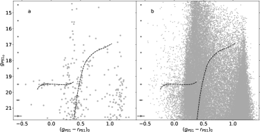
Figure 1: The CMD of all PS1 sources that pass our quality control cuts within (a) the half-light radius of the nominal center of Boo I (lefthand panel), and (b) a four-by-four degree area centered on Boo I (righthand panel). The locus of a PARSEC (Bressan et al., 2012) isochrone of age 13 Gyr, with [M/H]$=-2.2$, shifted by the distance modulus of Boo I, is over-plotted in dashed black lines in both panels. The symbol size of sources in the righthand panel is reduced, relative to the lefthand panel, for clarity.

After we completed the analysis presented below, the complementary analysis of Longeard et al. (2021) was posted to the arXiv. These authors similarly identify candidate Boo I member stars far from that galaxy’s center using a combination of photometry and Gaia astrometry. In their case they utilize the metallicity-sensitive photometric filters from the Pristine survey (see e.g. Starkenburg et al., 2017) and focus on RGB and HB stars redder than $(g-i)_{0,\,{\rm SDSS}}\sim 0.2$. There is no overlap between the sample of Longeard et al. (2021) and the candidate member stars identified using our technique below. We discuss the results from Longeard et al. (2021) further, within the context of our findings, in Section 4 below.

2 Photometric Identification of Candidate BHB and BSS Stars

Given a sample of blue stars, the identification of BHB stars, which have lower surface gravities than do main-sequence A-type stars of similar effective temperatures (and colors), through photometry has a long history and has evolved from UBV(RI) data (e.g., Newell, 1970; Wilhelm et al., 1999) to some combination of $ugriz$ (e.g., Yanny et al., 2000; Vickers et al., 2012). The technique essentially combines a color that is temperature-sensitive with one that is gravity-sensitive (in this range of effective temperature). The U-band ($u$-band) filter covers the Balmer jump which is higher in lower-gravity A-type stars, while the $z$-band filter covers the Paschen jump, which is similarly gravity-sensitive. We used photometry from the Pan-STARRS1 (PS1) survey, described in Chambers et al. (2016), which is well-suited to an analysis of the blue stellar content of Boo I, despite its lack of $u$-band information, as it has sufficient depth to study the blue-straggler stars (as demonstrated in Figure 1) and includes the $z-$band, which, as just noted, can be used to discriminate among A-type stars of differing surface gravities (Vickers et al., 2012). We will use the location of a given blue star in $griz$ color-color space to identify candidate BHB and BSS stars in Boo I. We did not utilize external $u$-band data, as we aimed to explore the utility of PS1 alone in the classification of blue sources. We compare the results of this $griz$-based analysis to those of a complementary $ugri$-based analysis in Appendix A.

2.1 Characterization of Different Stellar Sources in $griz$

Even with a sample selected to consist of only blue stellar-like objects, there are several additional source types that can occupy the blue side of color-magnitude diagrams such as those in Fig. 1, potentially contaminating a sample of the BHB and BSS of interest. These include background sources such as high-redshift, star-forming galaxies, AGN and quasars. Foreground main-sequence A-stars are unlikely at the relevant apparent magnitude range, particularly at the Galactic coordinates of Boo I ($\ell,\,b=358^{\rm o},\,+70^{\rm o}$). White dwarfs are likely, but their extremely high surface gravities (and their parallaxes, if available) should provide a means to identify them. Blue straggler stars and horizontal branch stars in the outer regions of the field halo of the Milky Way could also have colors and magnitudes close to those of actual Boo I members.

Guided by the earlier analyses of, for example, Sirko et al. (2004); Xue et al. (2008); Vickers et al. (2012), we quantified the loci occupied by different types of blue star-like sources in color-color space by combining the photometry with information from spectroscopy. We first selected all sources in the SDSS/SEGUE imaging data with ‘clean’ photometry (i.e. flagged as such in the database) and observed SDSS color $g-r\leq 0.1$. We then found the corresponding PS1 photometry for each source, using a maximum matching radius of one arc second. We implemented quality cuts, following those recommended by Flewelling et al. (2020), namely that the quality-of-fit parameter QfPerfect be greater than 0.85 for each of the four filters of this study ($griz$) and that the number of detections be greater than 5. We removed sources that were inconsistent with being stellar, based on their image shape and size compared to the point-spread function. We further restricted the sample to sources with extinction in the $g-$band less than or equal to 0.5 mag ($\sim 5\times$ the extinction along the line-of-sight towards Boo I), based on the dust maps of Schlafly & Finkbeiner (2011), and extinction-corrected the photometry for the remaining 16,205 sources, using the dustmaps package of Green (2018). We will refer to this cross-matched sample as the SEGUE-PS1 photometric catalog; its depth is determined by the SEGUE spectroscopic limit, at $g\sim 20$.

Figure 2: A plot of $(g_{PS1}-r_{PS1})_{0}$ color vs $\log~{}g$ for the set of stellar sources with surface gravity estimates from the SEGUE/SSPP and contained in the SEGUE-PS1 photometric catalog, derived as described in the text. The thick, dashed line at $\log\,g=3.75$ indicates the boundary that we adopted to separate BHB and BSS/MS stars. The thin, dotted, vertical red lines show the bluest and reddest extents of the color range adopted in the classification scheme developed in this paper.

The distribution in the log $g$ versus $(g_{PS1}-r_{PS1})_{0}$ color plane of the subset of sources from the SEGUE-PS1 photometric catalog which also have estimates of surface gravity from the SEGUE stellar parameter pipeline (SSPP) is shown in Figure 2. There is a clear separation into two clumps, characterized by surface gravity. The lower surface gravity stars are consistent with being BHB and the higher gravity stars are consistent with being main-sequence A-type stars (e.g. Bressan et al., 2012; Vickers et al., 2012). The horizontal thick, dashed line in Figure 2 at log $g=3.75$ indicates the dividing line in surface gravity that we used to assign blue stars to either of these two categories (the same threshold was adopted by Vickers et al., 2012). Specifically, we labeled the higher-gravity blue stellar sources (log $g>3.75$) as BSS/MS and the lower-gravity ones ($2.25\leq{\rm log}\,g<3.75$) as BHB. White dwarfs do not have an estimated surface gravity in the SSPP, but are flagged as such (‘D’) in the SEGUE database. Similarly, sources with emission lines, and therefore likely to be non-stellar, also lack an estimated surface gravity and are flagged (‘E’). We assigned the label ‘WD’ to all sources flagged as likely WDs and assigned the label ‘QSO’ to all flagged emission-line sources (remembering that all sources in our SEGUE-PS1 photometric catalog have been required to have blue colors and stellar image profiles). All remaining sources, of which there were 4274, we labeled as “other”; 11 are stars with gravity too low (log $g<2.75$) to be low-mass core-helium-burning BHB while the rest lack estimates for their atmospheric parameters for a variety of reasons. We did not consider any of these “other” sources in the analysis below.

The distribution of sources in the SEGUE-PS1 photometric catalog in the $(g_{PS1}-r_{PS1})_{0}$ versus $(i_{PS1}-z_{PS1})_{0}$ color-color diagram is presented in Figure 3, with each class identified by symbol type and color. The lefthand panel shows all sources we labeled as BHB, BSS/MS, WD, or QSO, while the righthand panel contains only the BHB and BSS/MS stars for which the SEGUE SSPP provided a low metallicity, specifically $\rm{[Fe/H]_{SSPP}}\leq-1.5$, approximately the maximum value found for stars in Boo I with spectroscopic abundances. While the metallicity distribution of stars in the metal-poor field halo, traced by the stars in the righthand panel, and that of Boo I differ, a comparison of the two panels of Figure 3 shows that metallicity has little impact on the loci occupied by the BHB and BSS/MS stars, affecting primarily the densities within the boundaries of those loci. We assumed below that this remains true even at extremely low values of the iron abundance, [Fe/H] $\sim-3$ dex, which is poorly represented within the SEGUE/SSPP sample.

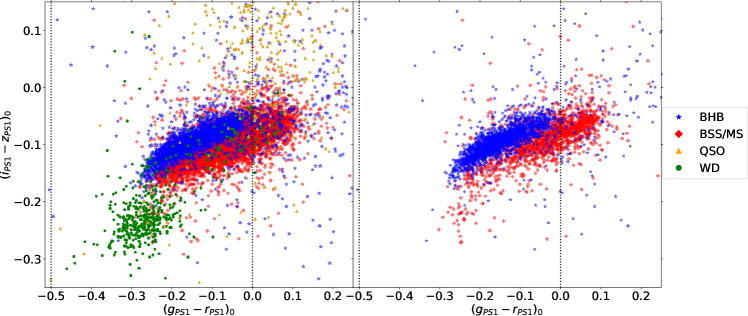
Figure 3: A $(g_{PS1}-r_{PS1})_{0}$ vs $(i_{PS1}-z_{PS1})_{0}$ color-color diagram of star-like sources in the SEGUE-PS1 photometric catalog for which we derived labels. The blue stars represent BHB stars, red diamonds represent BSS/MS stars, green circles represent WDs and orange triangles represent QSOs. All labeled sources are shown in the lefthand panel while the stars in the righthand panel are limited to those BHB and BSS/MS with metallicity estimates from the SSPP below $-1.5$ dex. The vertical dotted lines indicate the bluest and reddest extents of the color range adopted in this study.

Armed with this characterization of these different classes of source in $griz$ space, we now turn to the application of this knowledge to samples which lack spectroscopic atmospheric parameters, such as the sources observed along the line-of-sight to Boo I. As described below, we developed an automated classification technique that avoids subjective drawing of boxes in the color-color plane. We made the further restriction to consider only sources with colors in the range $-0.5\leq(g_{PS1}-r_{PS1})_{0}\leq 0$, which should encompass the expected BHB in Boo I  (see Figure 1), blueward of the instability strip.

2.2 K-Nearest Neighbors Classification

As may be seen in Figure 3, it is not straightforward to separate BHB from BSS/MS (hereafter BSS). We opted to use a k-nearest neighbors (KNN) classifier, which we trained on the SEGUE-PS1 photometric catalog. A KNN classifier acts first to identify the k objects (where k is some integer that the user is free to specify in order to optimize the process) in the training set that have the k smallest distances (in an appropriate sense) to a given input object, and then to classify the input object based on the labels of those k-nearest objects, providing the probability of each possible label.

We used the KNeighborsClassifier implemented in the Python package scikit-learn (Pedregosa et al., 2011). We trained this classifier on subsets of the SEGUE-PS1 photometric catalog, using all possible color combinations of the PS1 $griz$ photometry, such that the classifier worked in six-dimensional color space. The KNN classifier was then tested on the subsets of the catalog that were not used in the training; details of the training and testing are given in Appendix A, with only a brief summary here, outlining the procedure adopted and the success of the classifier.

The fractions of sources labeled as BSS, BHB, WD or QSO in the SEGUE-PS1 catalog are quite unequal, which could impact the classifier, so we first re-sampled the catalog to achieve a better balance between the classes (as described in more depth in Appendix A). We then split the re-sampled SEGUE-PS1 data randomly into test and training sets, where $70\%$ of the catalog was used to train the classifier and the other $30\%$ was used to test the classifier. We performed ten iterations of training and testing, in the six-dimensional color space, and in each iteration we used the same classifier parameters but a different re-sampling of the SEGUE-PS1 data. We then averaged the output of the ten iterations, and re-normalized the individual label probabilities for each source so they summed to unity. All probabilities given hereafter are these averaged, re-normalized values. We adopted a $50\%$ probability threshold for classification, i.e. for a source to be assigned to a given label, the probability for that label must be higher than $50\%$.

The completeness of a sample resulting from a classifier is generally defined to be the ratio of the number of sources that are correctly labeled to the true number of sources with that label (i.e., true positives divided by the sum of true positives and false negatives). Similarly, the purity is generally defined to be the ratio of the number of sources correctly labeled to the number of sources given that label (i.e., true positives divided by the sum of true positives and false positives). We found that, when applied to the test sets with known true stellar types, our KNN classifier produces samples of BHB that are, on average, $\sim 82\%$ complete and $\sim 81\%$ pure, together with samples of BSS that are, on average, $\sim 78\%$ complete and $\sim 80\%$ pure. These results are similar to, or better than, those obtained by previous broad-band color based techniques reported in the literature, such as that of Vickers et al. (2012) who used SDSS $griz$ photometry (they found $\sim 77\%$ purity and $\sim 51\%$ completeness for a sample of BHB stars).

The KNN classifier uses only color information, but as photometric errors are larger at fainter magnitudes, it is to be anticipated that its performance would decline with increasing apparent magnitude, as the larger uncertainties blur the distinction between BHB and BSS in color space. For reference, the average error in $(g_{PS1}-r_{PS1})_{0}$ color for blue sources at $g_{PS1_{0}}\sim 19$ is $0.02$ mag, increasing to $0.04$ mag at $g_{PS1_{0}}\sim 20$ and to $0.06$ mag at $g_{PS1_{0}}\sim 21$. We found that performance did indeed decrease towards fainter magnitudes, as illustrated in Figure 4, which shows the percentage completeness and false negatives for the selection of BHB and BSS as a function of apparent $g-$band magnitude.

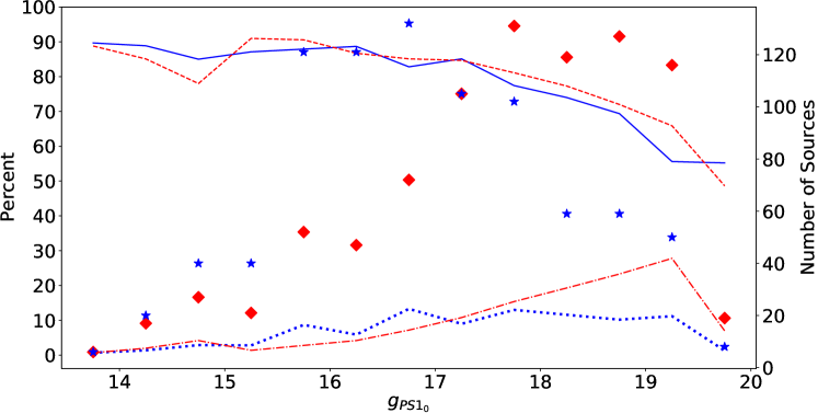
Figure 4: The average percentage completeness of BHB (solid blue line) and BSS (dashed red line) retrieved in each 0.5 magnitude-wide bin of apparent magnitude, together with the average percentages of true BHB that get labeled as BSS (blue dotted line) and vice-versa (red dash-dotted line). Note that these percentages are not guaranteed to sum to 100%, due to the small fractions of the BHB and BSS sources that were incorrectly classified as WD or QSO, or given no label with probability above 50$\%$. The blue stars and red diamonds represent the average number of BHB and BSS, respectively, in the test sets. In all cases, the values for bin centers are shown.

The purity achieved is of course sensitive to the relative numbers of BHB and BSS, as each is the main potential contaminant of the other (Starkenburg et al., 2019, see, for example Fig. 5 of). The average number of true BHB and BSS in each half-magnitude bin of the test sets is indicated by the points (stars and diamonds, respectively) in Fig. 4. These are determined by the structure of the Galaxy (a BHB star with an apparent $g-$magnitude of $19.75$ must be at a distance of $\sim 90$ kpc, while a BSS of the same apparent magnitude could be much closer), modulated by the complex selection function that results from first, the SEGUE survey, second, the cross-match described above, and third, the re-sampling discussed above. The populations of BHB and BSS in Boo I are most likely different from those in the training set, which has been adjusted to have equal proportions of BHB and BSS. Momany (2015) reports about twice as many BSS (of a broad range in magnitude) as (B)HB stars within the half-light radius of Boo I, using the photometry from Belokurov et al. (2006b) and assigning a star to a given type based purely on its location in the observed CMD. The BHB and BSS selected this way are separated in apparent magnitude, so it is difficult to make a comparison with the results in Fig. 4. Further, contamination of the CMD by Milky Way stars is difficult to quantify. Happily, Milky Way BHB and BSS stars can largely be removed from our sample of Boo I candidate members using astrometry.

2.3 Additional Tests of the KNN Classifier

We applied the KNN classifier to two datasets of known BHB stars (with spectra), the first being a different selection of BHB stars from SDSS/SEGUE by Xue et al. (2011) and the second being BHB with space motions consistent with membership of Boo I, taken from Koposov et al. (2011) and Jenkins et al. (2020).

2.3.1 The Xue et al. (2011) Sample

Xue et al. (2011) identified candidate BHB stars in a cross-matched sample of SDSS photometry and spectroscopy, using cuts based on both colors and the shapes of the Balmer lines (H$\delta$ and H$\gamma$). We cross-matched their catalog of candidate BHBs to the PS1 photometry, following the same procedure as for our own SEGUE-PS1 photometric catalog, yielding a sample of 4538 candidate BHB stars with $-0.5\leq(g_{PS1}-r_{PS1})_{0}\leq 0$. Application of our KNN classifier to this sample resulted in $89\%$ being labeled as BHB (adopting the $50\%$ probability threshold from above). Approximately $9\%$ of the stars in the sample are labeled as BSS stars, with the majority of the remaining stars ($\sim 2\%$ of the sample) being ambiguous, in that the classifier could not assign a probability higher than $50\%$ to any label.

Under the assumption that the Xue et al. (2011) catalog is entirely BHB stars (i.e. $100\%$ pure), the completeness obtained using our KNN classifier is comparable with that we obtained earlier. However, Lancaster et al. (2019) identified likely BSS candidates within the Xue et al. (2011) catalog, at the level of $\sim 10\%$ contamination and suggested refined restrictions in color and in the Balmer-line profiles to isolate the true BHB. We found that $\sim 7\%$ of the cross-matched sample would be identified as BSS using the criteria proposed in Lancaster et al. (2019) (ignoring their metallicity cut). Further, $48\%$ of the stars that our KNN classifier identified as BSS would be similarly classified by Lancaster et al. (2019), while 2$\%$ of those stars that our classifier identified as BHB would be identified as likely BSS with these refined criteria. This test revealed that some of the sources in the Xue et al. (2011) catalog that were “mis-classified” by our approach as BSS sources are, in fact, likely to be genuine BSS stars, and that the sample of BHB stars identified by our classifier has only a low level of contamination by these likely BSS stars, even though these BSS stars have properties similar enough to true BHB to be labeled as such using other techniques.

2.3.2 Spectroscopic BHB members of Boo I

We cross-matched the catalog of sources observed spectroscopically by Koposov et al. (2011) (re-analyzed by Jenkins et al., 2020) with the PS1 photometric dataset, following the same criteria for matching radius and photometric quality outlined above. All six of the non-variable BHB candidates (based on location in the CMD) targeted by Koposov et al. (2011) met the membership criteria of Jenkins et al. (2020), including having consistent proper motion from Gaia EDR3, and all six have matches with high-quality photometry in PS1. Application of the KNN classifier to these six sources resulted in five of the stars being labeled as BHB and one being labeled as a BSS star. This $83\%$ completeness is consistent with the overall performance of the classifier, and is higher than the completeness seen for Milky Way halo BHB stars at a comparable faint magnitude, $g_{PS1_{0}}\sim 19.5$, in Figure 4. The star mislabeled as a BSS star lies in a region of color-color space occupied by both BSS and BHB (its location is marked by the open black circle symbol in the lefthand panel of Figure 5) and indeed, approximately ten times as many BSS than BHB in the training set have similar colors (defined as all six colors being within $\pm 0.015$ of those of the misclassified BHB).

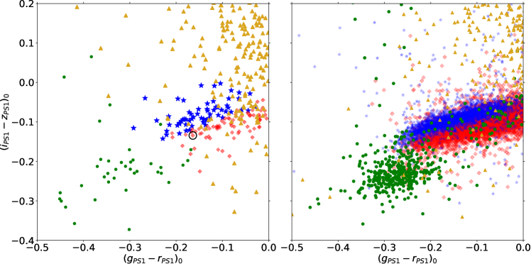
Figure 5: The $(g_{PS1}-r_{PS1})_{0},(i_{PS1}-z_{PS1})_{0}$ distribution of the labeled Boo I catalog sources (lefthand panel), compared to the distribution of the SEGUE-PS1 cross-matched catalog sources (righthand panel). BHB are shown as blue stars, BSS/MS as red diamonds, WD as green circles, and QSOs as orange triangles. For clarity, the size and opacity of the symbols representing the BSS and BHB sources on the SEGUE-PS1 plot are reduced relative to those of the Boo I field plot. The BHB from the Koposov et al. (2011) and Jenkins et al. (2020) sample that is mis-classified as a BSS star is indicated with an open black circle in the lefthand panel.

Perhaps unsurprisingly given their photometric variability, the classifier also mislabeled the 5 RR Lyrae associated with Boo I that had blue enough PS1 colors and sufficiently high-quality photometry to be included in the sample: three were classified as QSO, one as a BSS, and one was unclassified (no label was assigned with probability above 50%).

2.4 Selection of Blue Stars in a Wide-Area Boötes I Field

We investigated the existence of an extended stellar envelope of Boo I by first selecting all sources with high-quality 4-band PS1 photometry, and with positions within a four-by-four degree box around the coordinates of the nominal center of Boo I. The area selected encompasses more than $\sim 100$ times that enclosed by the (elliptical) half-light isophote of Boo I ($\lower 2.15277pt\hbox{$\;\buildrel<\over{\sim}\;$}0.1$ square degree, based on the exponential fit to the surface density profile from Muñoz et al. 2018) and allows exploration of the stellar content well beyond the King profile nominal tidal radius of Boo I. We imposed the same quality-control requirements on the photometry as described above, ensuring that each source has point-like photometry in each filter, and again corrected the photometric data for dust reddening and extinction. The resultant photometric dataset is composed of sources brighter than $g\sim 22$ ($\sim 2.5$ magnitudes fainter than the expected magnitude of BHB at the distance of Boo I, see below) and is hereafter referred to as ‘the Boo I catalog’. Any possible non-uniformity in the limiting magnitude of this catalog should affect the completeness of only the BSS sample, and these sources are sufficiently faint that the decreasing performance of the KNN classifier with apparent magnitude significantly impacts the completeness (see Figure 4). Happily, our science goals do not require a complete sample of BSS and we did not attempt to correct for incompleteness.

We then applied the (trained) KNN classifier to the Boo I catalog, again requiring a minimum probability of $50\%$ for a given label to be assigned to a source. Of the 437 sources in the Boo I catalog with $-0.5\leq(g_{PS1}-r_{PS1})_{0}\leq 0$, the classifier labeled 62 as BHB and 76 as BSS (see Table 1). Of the remaining sources, 52 were labeled as WD, 225 were labeled as QSO, and 22 were ambiguous. Fainter than $g_{PS1_{0}}\sim 21$, no source was labeled as either BHB or BSS. This likely reflects the trend of decreasing completeness at fainter magnitudes seen in Figure 4.

The distribution of all the classified star-like sources in the $(g_{PS1}-r_{PS1})_{0},(i_{PS1}-z_{PS1})_{0}$ color-color plane is shown in Figure 5, where the lefthand panel displays the sources in the Boo I catalog that were successfully labeled (i.e. with probability greater than 50%) and the righthand panel displays the distribution of the SEGUE-PS1 cross-matched catalog, in which case the labels were based on the SEGUE spectroscopy, as described above in Section 2. The loci occupied by the different types of source are similar in the two panels, albeit that there is a higher relative number of QSO in the lefthand panel (the Boo I catalog). This increased presence of QSOs plausibly reflects the combined effects of the higher fraction of extragalactic sources compared to Galactic stars at the deeper limiting magnitude of the Boo I catalog, the increased misclassificaton of sources at fainter magnitudes due to larger photometric errors, and the SEGUE selection function. The majority ($68\%$) of these sources labeled as QSO are fainter than $g_{PS1_{0}}=20$, the limiting magnitude of the SEGUE-PS1 catalog.

The subset of sources classified as either BHB or BSS in the Boo I catalog includes field stars in the Milky Way, in addition to actual members of Boo I. The Milky Way stars should span a broad range of apparent magnitudes, reflecting their (unknown) distances, while the member stars of Boo I should be constrained to a narrower range of apparent magnitudes, consistent with the known distance to Boo I and their intrinsic luminosities.

The large metallicity spread of Boo I ($\Delta[\rm{Fe}/\rm{H}]\sim 1.7$ dex, e.g. Norris et al. 2010a) should cause some spread in the absolute magnitude of BHB (at fixed color). The recent calibration by Fermani & Schönrich (2013, their equation 5), valid over the range $-3\lower 2.15277pt\hbox{$\;\buildrel<\over{\sim}\;$}{\rm[Fe/H]}\lower 2.15277pt\hbox{$\;\buildrel<\over{\sim}\;$}-1$, would imply a spread of $\sim 0.15$ mag in absolute $g$-magnitude at a color of $(g-r)_{SDSS}=-0.15$, for a metallicity distribution similar to that of Boo I. Empirically, the BHB fiducials of globular clusters of very similar iron abundances vary by a similar, or even larger amplitude in absolute magnitude - for example, Bernard et al. (2014) found a range of $\lower 2.15277pt\hbox{$\;\buildrel<\over{\sim}\;$}0.3$ magnitudes for the BHB in a set of four metal-poor globular clusters, with iron abundance varying by only $\sim 0.1$ dex. Further, the uncertainty in the distance estimate given by Okamoto et al. (2012) ($65\pm 3$ kpc), translates to an uncertainty of 0.2 in apparent magnitude, for given absolute magnitude. Given these considerations, we decided to define the apparent magnitude range of the BHB in Boo I by the 13 Gyr, ${\rm[M/H]=-2.2}$ PARSEC isochrone, shifted by a distance modulus corresponding to 65 kpc, and allowing a spread of $\pm 0.2$ magnitudes, vertically, about the locus of the HB set by the isochrone (the uncertainty in the PS1 photometry at the magnitudes of interest, indicated on Figure 1, is small in comparison). We confirmed that all of the six BHB members from Jenkins et al. (2020) lie within these boundaries.

The BSS systems of a given stellar population will have a range of absolute magnitudes, depending on the (uncertain) details of their formation mechanism(s), but for an old population Hurley et al. 2005; Geller et al. 2013 they should be fainter than the horizontal branch and indeed be within a couple of magnitudes brighter than the main-sequence turnoff (MSTO). This expectation is consistent with the predicted brightness of an unevolved main-sequence star of mass equal to twice that of the old turn-off, which is $\sim 2$ magnitudes brighter than the turn-off in the $g-$band ($1.93$ magnitudes with our fiducial isochrone). Further, the observed BSS populations of globular clusters, in the cases where proper motions are available to confirm membership, are within $\sim 2.5$ magnitudes of the turn-off (Baldwin et al., 2016). The MSTO of Boo I, defined by the bluest point of our fiducial isochrone, corresponds to $g_{PS1_{0}}=23.07$. Adopting the metal-poor globular cluster M92 as an empirical fiducial and using the data from Bernard et al. (2014) predicts a MSTO for Boo I of $g_{PS1_{0}}=23.1$, in excellent agreement. We therefore identified candidate BSS members of Boo I by requiring that they have apparent magnitude fainter than $g_{PS1_{0}}=23.1-2.5=20.6$ (this cut removes the mis-classified BHB and RR Lyrae members). Note that the faintest BSS in our sample should then be at the $g_{PS1_{0}}\sim 22$ limit set by the stringent quality controls we implemented on the multi-band photometry.

There are 25 candidate BHB and 4 candidate BSS selected by this step, with the projected spatial distribution as shown in Figure 6 (righthand panel). The other panels of Fig. 6 show, for comparison, the distribution of all the blue sources in the Boo I catalog (lefthand panel) and that of all sources, independent of apparent magnitude, labeled as either BHB or BSS (middle panel). The selection region used to delineate the appropriate ranges of apparent magnitudes and colors for BHB stars at the distance of Boo I is shown in Figure 7, over-plotted on the CMD of the blue sources in the Boo I field. Each different class of source, as labeled by our KNN classifier, is indicated by symbol type and color (as described in the figure caption). The final set of candidate BHB member stars (including proper-motion cuts as described below) and those apparent magnitude-appropriate BSS are indicated with larger symbols.

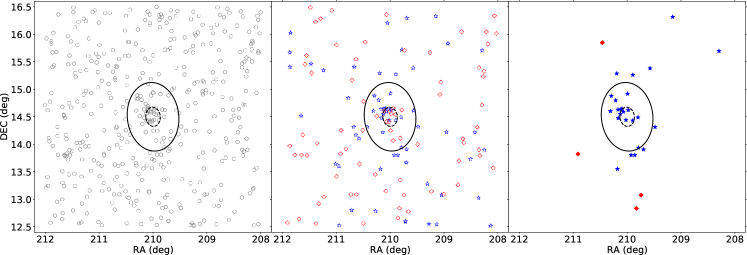
Figure 6: The two-dimensional spatial distribution of various subsets of blue sources in the field of view of Boo I, together with the King profile tidal and exponential half-light ellipses of Muñoz et al. (2018) (black solid and dashed lines, respectively). The leftmost plot shows all sources with $-0.5\leq(g_{PS1}-r_{PS1})_{0}\leq 0$, the middle panel shows all BHB or BSS stars, and the rightmost panel shows the subset of BHB and BSS stars that have apparent magnitudes that are consistent with the expected magnitudes of BHB and BSS at the distance of Boo I.

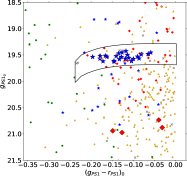
Figure 7: The CMD of blue sources in the Boo I field, color-coded by the label assigned by the classifier. BHB stars are shown as blue stars, BSS as red diamonds, WD as green circles, QSO as orange triangles, and ambiguous sources with no label having higher than $50\%$ probability are shown as grey crosses. The isochrone-based selection region used to identify BHB stars with appropriate apparent magnitudes is outlined in black. We verified via proper motion that the bright BHB just above this region is unlikely to be a member of Boo I. The BHB that do have consistent proper motions are shown with larger symbols, as are the BSS that pass our imposed magnitude cut for potential members ($g_{PS1_{0}}>20.6$). The sources with ambiguous classifications within the BHB selection region are discussed further in the text.

Some Milky Way field stars could make it through these photometric cuts and we implemented further astrometric cuts, as described in Section 3.

2.5 Selection of Blue Stars in Comparison Off-Fields

We selected four lines-of-sight at comparable Galactic coordinates to Boo I, to define ‘off fields’ within which to estimate the contamination of the sample of BHB and BSS obtained above, by non-members of Boo I. Boo I is located in the ‘Field of Streams’ (Belokurov et al., 2006a) and we took considerable care to minimize contributions in the off-fields from the Sagittarius (Sgr) streams, by inspection of the proper motions of all sources in the field (a nearby fifth field which shows a clear signature of Sgr in the proper motions is discussed in Appendix C). The coordinates of the centers of the off-fields we selected are given in Table 1 and the locations on the sky of these $4\times 4$ square degree fields, plus the fifth (Sgr stream) field, are illustrated in Figure 8. From analytic models of Milky Way stellar density profiles, we would not expect significant dependence of the surface density of faint blue stars on Galactic latitude over the range of field-center coordinates considered in this work. Indeed, the TRILEGAL models (Girardi et al, 2005) predict only a $\lesssim 20\%$ difference of the surface densities of faint blue stars (which we defined to be $-0.5\leq(g_{PS1}-r_{PS1})\leq 0$, $19<g_{PS1}<21$ in the extinction-free, error-free synthetic magnitudes provided by TRILEGAL) between fields centered on $(\ell,b)=(355,70)$ and $(\ell,b)=(355,85)$. We thus proceeded with the selected observational off-fields.

Figure 8: The on-sky footprints of the four main off-fields considered in this work, together with the Boo I field and the additional rejected off-field that is contaminated by stars from the Sagittarius stream. The BHB stars that have both proper motions and apparent magnitudes consistent with membership of Boo I are shown as blue stars.

We applied the KNN classifier to the blue star-like sources in each off-field, after obtaining photometric catalogs following the procedure detailed above. The resultant numbers of BHB and BSS are given in Table 1, where the two rightmost columns indicate the numbers of BHB and BSS with appropriate apparent magnitudes to be at the heliocentric distance of Boo I (assumed to be 65 kpc; Okamoto et al., 2012). Inspection of Table 1 shows that the number of stars in each off-field that are classified as BHB and have photometry consistent with being at the distance of Boo I is approximately constant field-to-field (with the exception of off-field 1), at a level of $10-20\%$ of the BHB in the Boo I field. The implied surface density of BHB in the field stellar halo of $\sim 1$ BHB per 4 square degree at a distance of $\sim 65$ kpc is somewhat higher than the count of 3 BHB in 40 square degree, at distances of $50-100$ kpc, found by Deason et al. (2018) in lines-of-sight away from both the Sgr stream and the VVDS over-density. This apparent disagreement is perhaps unsurprising, given that the selected off-fields are in close proximity to known over-densities, which were explicitly avoided in Deason et al. (2018). It may be expected that such field halo BHB should be on different orbits about the Galactic center than are the BHB members of Boo I, even if at similar Galactocentric distance, and so should be distinguishable by kinematics, which we turn to next.

Table 1: Field Centers and Blue Star Counts

Name	$\ell$	$b$	RA	Dec	All Blue	All BHB	All BSS	BHB	BSS
			(J2000)	(J2000)
Boo I	358.0∘	69.6∘	210.00∘	14.50∘	437	62	76	25	4
Off-Field 1	358.1∘	75.0∘	205.75∘	18.00∘	389	42	53	6	2
Off-Field 2	357.7∘	85.0∘	197.30∘	24.20∘	331	48	37	2	1
Off-Field 3	352.0∘	79.5∘	201.28∘	20.00∘	424	47	55	4	1
Off-Field 4	15.0∘	70.0∘	213.06∘	19.56∘	344	42	52	2	1

Note. — All fields are $4\times 4$ sq. degree. The column ‘All Blue’ gives the number of star-like sources within that field with high-quality PS1 photometry and with $-0.5\leq(g_{PS1}-r_{PS1})_{0}\leq 0$. ‘All BHB’ and ‘All BSS’ give the subsets of the blue stars that are so classified, and ‘BHB’ and ‘BSS’ give the further subsets that have appropriate apparent magnitudes to be at the distance of Boo I.

3 Astrometric Identification of Likely Boo I Members

The Gaia EDR3 astrometric catalog is sufficiently precise and accurate at the apparent magnitudes of interest that it can be utilized both to determine the mean proper motion of Boo I and then to isolate potential Milky Way contaminants in the photometrically selected, apparent-magnitude consistent BHB sample. We first cross-matched the PS1 photometric catalogs for each of the fields in Table 1 with the Gaia EDR3 data (querying the gaia_source catalog), using the functionalities provided in TOPCAT (Taylor, 2005). We required that the Gaia data for each source were well-fit by a single-star model (ruwe $<1.3$), the astrometric solution was derived over at least 6 visibility periods (visibility_periods_used $>6$), and the photometry was not significantly affected by background light or blending (thus requiring that the photometry satisfy the relation $1.0+0.015(\rm{G_{BP}}-\rm{G_{RP}})^{2}<$ phot_bp_rp_excess_factor $<1.3+0.06(\rm{G_{BP}}-\rm{G_{RP}})^{2}$, as recommended by Gaia Collaboration et al., 2018).

3.1 Derivation of the Mean Proper Motion of Boötes I

We derived our own estimate of the mean proper motion of Boo I, in order to create an internally consistent sample of proper-motion members, from which we defined a covariance ellipse that we used to identify new, astrometrically consistent, candidate members. We defined the mean proper motion using the Gaia EDR3 astrometry (Gaia Collaboration et al. 2016, Gaia Collaboration et al. 2020) for stars that had been previously identified, primarily through spectroscopy, as members. We used the samples of Martin et al. (2007), Norris et al. (2010a), and Koposov et al. (2011) to compile a catalog of stars that have, at a minimum, line-of-sight velocity consistent with membership. We supplemented this with the full set of 16 RR Lyrae variables identified by Siegel (2006) and/or Vivas et al. (2020) as being associated with Boo I; any found not to have consistent proper motions would be removed though the process described below (as noted above the Gaia DR2 proper motions suggested one was a non-member). Most of this combined sample lies within the half-light radius of Boo I, although two members on the RGB from Norris et al. (2010a) and two of the RR Lyrae stars lie beyond the King profile nominal tidal radius.

There is some overlap among the spectroscopic samples and there is not always agreement in the published results as to the membership status of a given star. We proceeded by assigning our own membership value of unity to every star indicated as a member of Boo I in each study, and a membership value of zero to stars indicated as non-members in that study. The spectroscopic data for the sample observed by Koposov et al. (2011) was re-analyzed by Jenkins et al. (2020) and we adopted the membership criteria developed by the latter authors. We averaged the membership values for any star in more than one sample, removed the duplicate entries and matched the resulting catalog of unique stars to both the PS1 photometry and the Gaia EDR3 catalog.

We considered all stars with an averaged membership value of $\geq 0.5$ to be actual members of Boo I  and we derived the mean proper motion of Boo I from only the subset of these members brighter than $G_{Gaia}=20$, for which the proper motion uncertainties are $\lower 2.15277pt\hbox{$\;\buildrel<\over{\sim}\;$}0.5$ mas yr^-1. We note that none of these member stars has a robust parallax measurements in Gaia EDR3 (all have have parallax errors larger than $20\%$), indicating that none is likely to be a nearby foreground star. We calculated the median of the proper motions in each of right ascension and declination ($\mu_{\alpha*},\,\mu_{\delta}$, with the usual convention that the $*$ indicates the cosine of declination), and then removed all stars with proper motions outside of the three-sigma covariance ellipse defined by the initial sample of bright members. We then repeated this process, iteratively defining the median and rejecting stars outside of the new three-sigma covariance ellipse, until no further stars were rejected. We used the final set of surviving members (59 stars) to determine the mean proper motion of Boo I, which we defined as the error-weighted average of the proper motions of each of those stars. We further adopted the three-sigma covariance ellipse from this final set of stars as the proper motion ellipse of Boo I.

The mean proper motion of Boo I defined by this iterative process is $\mu_{\alpha*}=-0.397\pm 0.019$ mas yr^-1, $\mu_{\delta}=-1.066\pm 0.015$ mas yr^-1. These values are in excellent agreement with the Gaia EDR3-based proper motion determination of McConnachie & Venn (2020) ($\mu_{\alpha*}=-0.39\pm 0.01$ mas yr^-1, $\mu_{\delta}=-1.06\pm 0.01$ mas yr^-1) and is within two sigma of the EDR3-based proper-motion values found by Li et al. (2021) ($\mu_{\alpha*}=-0.307\pm 0.052$ mas yr^-1, $\mu_{\delta}=-1.157\pm 0.043$ mas yr^-1), by Martínez-García et al. (2021) ($\mu_{\alpha*}=-0.357\pm 0.029$ mas yr^-1, $\mu_{\delta}=-1.071\pm 0.024$ mas yr^-1), and by Battaglia et al. (2021) ($\mu_{\alpha*}=-0.369\pm 0.039$ mas yr^-1, $\mu_{\delta}=-1.071\pm 0.029$ mas yr^-1). We used the mean proper motion (plus line-of-sight velocity and distance) to derive orbital parameters for Boo I in two different Milky Way potentials, as described in Appendix B. It should be noted that the favored orbit for Boo I adopted in the analysis of Fellhauer et al. (2008) is remarkably similar to that found here, despite no proper-motion information being available to those authors.

3.2 Selection of Proper-Motion Consistent Member Stars

We defined a star to be “proper motion consistent” provided that the error ellipse of its reported proper motion intersected with, or was contained by, the three-sigma covariance ellipse defined by the set of 59 stars used above to determine the mean proper motion of Boo I. We found that approximately $30\%$ of all the blue stars, independent of apparent magnitude range, in the Gaia-PS1 cross-matched catalog for the Boo I field have proper motions consistent with membership of Boo I, compared to only $\sim 20\%$ of all the blue stars in each of the Gaia-PS1 catalogs for the off-fields. As such, the majority of non-member contaminants can be identified by their proper motions ($\sim 80\%$, assuming all stars in the off-fields are non-members), which allows for the refinement of the candidate-member catalog that was obtained based on photometry alone.

3.2.1 BHB Candidate members in the Boo I Field

Of the 25 stars in the Boo I field that were identified by the KNN classifier as candidate BHB and which also have appropriate magnitudes to be at the distance of Boo I, 24 have consistent proper motions. We verified that none of these 24 stars has a robust measurement of parallax in Gaia EDR3 all have parallax error larger than $20\%$) and thus none is likely to be a nearby foreground star. The BHB that was rejected on the grounds of having inconsistent proper motion is only slightly outside of our (rather generous) proper-motion bounds, and could be considered proper-motion consistent in the future, depending on improved astrometry from future Gaia data releases. As seen in Figure 7, there are seven ambiguous sources (indicated by grey crosses) with colors and magnitudes that place them within the selection region for BHB stars in Boo I. Three of these ambiguous sources have proper motions consistent with Boo I, two of which are located interior to the King profile nominal tidal radius, each with BHB label probability below $\sim 45\%$. The third source lies beyond the King profile nominal tidal radius but has only a $\sim 30\%$ probability of being a BHB star, and thus is unlikely to be a genuine BHB member of Boo I.

Five of the six BHB stars from the Koposov et al. (2011) and Jenkins et al. (2020) sample survive the iterative clipping we used to define the three-sigma covariance ellipse, while all six meet the criterion to be considered proper-motion consistent. This apparent inconsistency arises due to the fact that while the errors in proper motion are not considered in the definition of the three-sigma covariance ellipse, they are taken into account when considering whether or not an individual star could be a member. Thus five of the BHB stars have proper motion measurements that lie inside of the ellipse, while the proper-motion measurement of the sixth lies outside, but with an error ellipse that intersects the three-sigma covariance ellipse.

3.2.2 Boo I Field BSS Candidate members

Our requirement that BSS candidates be no more than 2.5 magnitudes brighter than the dominant old MSTO, which for Boo I corresponds to $g_{PS1_{0}}>20.6$, means that they are unlikely to have Gaia EDR3 astrometric data (limiting apparent magnitude $G_{Gaia}\sim 21$) of high enough quality for membership tests. This is indeed the case, and none of the candidate BSS members in the Boo I field, identified using photometry alone, can be included in the sample of proper-motion consistent candidate member stars.

3.2.3 Variable Stars in Boötes I

The 16 RR Lyrae variables associated with Boo I by Siegel (2006) and by Vivas et al. (2020) were included in the initial stage of the iterative procedure we used to define the mean proper motion of Boo I, and three of these stars were rejected in the sigma-clipping step. However, all 16 RR Lyrae stars have proper motions consistent with membership of Boo I when their errors are considered (similar to the situation for the six BHB from Koposov et al., 2011 discussed above). This set of stars provides a graphic illustration of the improvement in the astrometric data for evolved stars in Boo I between Gaia DR2 and EDR3. Figure 9 shows the comparison between the proper motions for the RR Lyrae based on DR2 (lefthand panel) and on EDR3 (righthand panel). The three-sigma covariance ellipse indicated on each panel was defined through the iterative sigma-clipping procedure described above and based on an input list of candidate members that included the RR Lyrae themselves. The EDR3 data yield reduced scatter in the distribution of proper motions and considerably smaller individual error bars. Further, the RR Lyrae star that was rejected by Vivas et al. (2020), based on DR2, is retained using EDR3. The two RR Lyrae at projected radii beyond the King profile nominal tidal radius are indicated by special symbols in Figure 9 (a pink square for the candidate from Siegel, 2006; an orange diamond for that from Vivas et al., 2020).

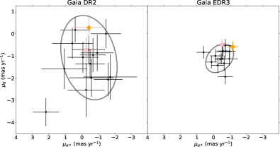
Figure 9: The proper motions from Gaia DR2 (lefthand panel) and EDR3 (righthand panel) for the RR Lyrae stars identified by Siegel (2006) and Vivas et al. (2020). The error bars correspond to the quoted uncertainties in the proper motions for each source in the DR2 or EDR3 catalog. The three-sigma covariance ellipse for each dataset, defined through iterative sigma-clipping of previously identified member stars, is shown in grey. The pink square indicates the outer envelope RR Lyrae star from Siegel (2006) while the orange diamond indicates the additional outer envelope RR Lyrae from Vivas et al. (2020).

In addition to RR Lyrae variables, a candidate LPV member was identified by Siegel (2006) and Dall’Ora et al. (2006), as noted above. The coordinates of this LPV star place it within the half-light ellipse of Boo I and we found its proper motion in Gaia EDR3 to be consistent with that of Boo I, again indicating likely membership. We identified an object with matching coordinates in the general LAMOST catalog (see Cui et al., 2012; Zhao et al., 2012). The signal-to-noise of the spectrum (obsid 230716130) is sufficiently low that only a redshift is reported, with value $0.00028465\pm 0.0000433$. The corresponding heliocentric velocity, $\sim 85\pm 13$ km s^-1, is consistent with membership of Boo I (mean velocity of $\sim 100$ km s^-1; Jenkins et al., 2020), but this interpretation must be treated with caution due to both the low signal-to-noise ratio and the inherent difficulties/uncertainties in measuring the center-of-mass velocity for pulsating stars (see, e.g. Lebzelter & Hinkle, 2002). We identified a source with matching coordinates in the 2MASS catalog (2MASS $13594873+1434483$). This source has a J-K_s color of $0.8$, indicating that it is unlikely to be an AGB star with a very dusty envelope (see e.g. Nikolaev & Weinberg 2000). The most metal-poor LPV stars discovered to date reside within the globular cluster M15 (NGC 7078; McDonald et al., 2010), which has an iron abundance of $[\rm{Fe/H}]=-2.29$ (Bailin, 2019), some $\sim 0.3$ dex higher than the mean iron abundance of Boo I (mean $[\rm{Fe/H}]=-2.6$, Frebel et al., 2016). Should this LPV star be a true member of Boo I, it could also be the most metal-poor LPV discovered. This exciting possibility warrants additional investigation.

3.2.4 Boötes II

The Boötes II UFD (hereafter Boo II) has central coordinates of ${\rm(RA,Dec)=(209^{\circ}.50,12^{\circ}.85)}$ (Walsh et al. 2007) and thus lies within the four-by-four degree Boo I field explored in this work. Boo II is closer than Boo I, with a heliocentric distance of $42\pm 1.6$ kpc (Walsh et al., 2008), and has a higher proper motion ($\mu_{\alpha*},\mu_{\delta}=-2.273\pm 0.151,-0.361\pm 0.115$ mas yr^-1, Li et al. 2021). Contaminants from Boo II within the sample of candidate Boo I members is thus unlikely. Indeed, inspection of Figure 6 shows that there are no apparent-magnitude consistent BSS or BHB within $\sim 0.3$ degree of the center of Boo II ($\sim 6$ half-light radii, adopting the exponential half-light radius of $3.07\pm 0.44$ arcmin for Boo II from Muñoz et al. 2018).

3.2.5 Proper-Motion Consistent Blue Member Stars in the Boo I Field

The proper-motion consistent BHB stars identified earlier in this section form our final sample of candidate members among the blue stars (see Table 2). Their positions and proper motions are illustrated in Figure 10, with arrows indicating the directions and magnitudes of the individual proper motions (the length of the arrows have been scaled automatically by the mean of the magnitudes of the individual proper motions, in combination with sample size, for clarity). The positions on the sky of these candidate BHB members, together with previously identified proper-motion consistent member stars are shown in Figure 11, with the righthand panel being a zoom-in of the inner regions, where the bulk of the spectroscopic members are located. The RR Lyrae from Siegel (2006) and Vivas et al. (2020), in addition to the non-variable BHB stars from Koposov et al. (2011) and Jenkins et al. (2020) are indicated by different symbols. The ellipses in both Figure 10 and Figure 11 indicate the half-light radius and King profile tidal radius from Muñoz et al. (2018).

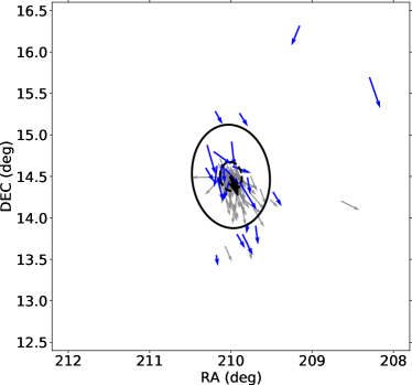
Figure 10: Gaia EDR3 proper motions of previously identified member stars (grey arrows) and of the candidate BHB member stars from this work (blue arrows). The mean proper motion of Boo I  is shown as a thick black arrow (not to scale) and the King profile tidal and half-light ellipses of Muñoz et al. (2018) are shown in black solid and dashed lines, respectively. The lengths of the arrows indicating the individual proper motions have been scaled, for clarity, by the magnitude of the mean proper motion, in combination with the sample size .

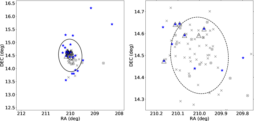
Figure 11: The two-dimensional distribution of candidate BHB (blue stars) members of Boo I, over-plotted on the King profile tidal and exponential half-light ellipses of Muñoz et al. (2018) (black solid and dashed lines, respectively). Previously identified member stars that have proper motions consistent with Boo I are shown as grey crosses, open grey circles around crosses indicate that the source is a literature RR Lyrae, and open triangles around the crosses indicate that the source is a non-variable literature BHB (from Koposov et al. 2011 and Jenkins et al. 2020).

3.3 Proper-motion Consistent Stars in Off-Fields

We find between 1 and 4 proper-motion consistent, apparent-magnitude appropriate BHB stars in each of the off-fields (see Table 2). Unlike the Boo I field, two of the off-fields each contain one apparent-magnitude consistent BSS star with a Gaia counterpart, but neither of these stars has a proper motion consistent with that of Boo I.

The assumption that these BHB candidates in the off-fields are actually members of the field stellar halo at distances similar to Boo I  and are distributed approximately uniformly across the sky on $\sim 10^{o}$ scales implies we could thus expect $\sim 2$ stars in the catalog of candidate BHB members to be non-members, or a $<10\%$ contamination level even after imposing a proper-motion cut. On the other hand, they could be actual members of Boo I in a very extended envelope. The location of Boo I on the sky, in projection against the ‘Field of Streams’, complicates investigations on the structure of Boo I on these larger angular scales, as illustrated in Appendix C. In the limit of a smooth and symmetric stellar halo, the counts of faint BHB in the Milky Way halo should be the same for fields at the same Galactocentric distance, and an alternative approach is to investigate the BHB content of the field halo far from the line-of-sight of Boo I, using our technique to classify stars. We adopted Galactocentric Cartesian coordinates, with the Sun located at (X_⊙, Y_⊙, Z_⊙) = ($-8.3$, 0, 0.27) kpc and Boo I at (X_boo, Y_boo, Z_boo) = (14.50, $-0.80$, 60.9) kpc. We selected a line-of-sight approximately 180^∘ from Boo I (and thus towards the Galactic anticenter) by changing the sign of the X-coordinate, and sought to identify BHB stars at the same Galactocentric distance as Boo I (62.6 kpc). We thus applied our classifier to the PS1 data in a $4\times 4$ degree field centered on Galactic coordinates ($\ell,\,b$) = (187^∘, 84^∘), and restricted the apparent magnitude range to isolate BHB along this line-of-sight with Galactocentric (X, Y, Z) coordinates of ($-14.5$, $-0.8$, 60.9) kpc. We found that this field contained fewer BHB stars (27) of any apparent magnitude than did any of the other fields we considered and that there were zero BHB at the same Galactocentric distance as Boo I, allowing for the same selection box as above. The status of the few BHB in the more local off-fields that have astrometry consistent with being members of Boo I thus remains ambiguous.

3.4 Comparison with CMD-based Membership Criteria

The estimated $\lesssim 10\%$ contamination level of the final proper-motion consistent, KNN-classified sample of BHB associated with Boo I is significantly lower than that which would be achieved via selection of stars based on their location on the CMD. For example, if we were to select all blue stars with g-band apparent magnitude within $\pm 0.2$ mag of the horizontal branch predicted by our chosen PARSEC isochrone, on the $(g_{PS1}-r_{PS1})_{0}$ vs $g_{PS1_{0}}$ CMD of the Boo I field, the resulting sample would contain sixty-three potential BHB members. stars. Application of this criterion to the CMDs of the off-fields would provide samples of between twenty-eight and thirty-six stars. The assumption that these stars in the off-fields are non-members of Boo I and that there would be a similar number ($\sim 33$) of non-member stars in the Boo I field, implies that using only a CMD-based selection cut to identify candidate BHB member stars of Boo I would be likely to produce a catalog that had $\sim 50\%$ contamination, from primarily Milky Way stars plus background QSOs.

Note that this estimated $\sim 50\%$ contamination rate for CMD-selected candidate BHB is entirely consistent with the fact that all of the candidate member BHB stars selected using this method and observed spectroscopically by Koposov et al. (2011) have radial velocities and proper motions consistent with membership of Boo I (Jenkins et al., 2020). The stars in this spectroscopic BHB sample are located within or near the half-light radius of Boo I, where the contrast between Boo I members and the field stellar halo is highest (see Figure 11). The expected identification rate of non-member BHB candidates based on the off-fields, $\sim 33$ per 16 sq. degree field, would predict between zero and one such contaminant within the area enclosed by the half-light radius of Boo I ($r_{h}\lower 2.15277pt\hbox{$\;\buildrel<\over{\sim}\;$}10.5$ arcmin).

Table 2: Candidate Member BHB Per Field

Field Identifier		PM Consistent BHB
Boo I		24
Off-Field 1		4
Off-Field 2		1
Off-Field 3		2
Off-Field 4		2

Note. — Counts of apparent-magnitude appropriate BHB stars which also have proper motion consistent with that of Boo I.

4 Discussion

The candidate member stars identified in this work form an extended envelope of blue stars, the two-dimensional distribution of which is presented in Figure 11, together with previously identified members taken from the literature. The King profile tidal and exponential half-light ellipses of Boo I from Muñoz et al. (2018) are indicated for reference. It is evident that the King profile tidal radius does not mark the edge of the member stars, a possibility discussed in Roderick et al. (2016). Indeed, our new BHB candidates extend to beyond ten half-light radii from the center of Boo I, out to $\sim 122$ arc minutes, or $\sim 2.3$ kpc. The distribution of these candidate BHB members is generally aligned with the inner isophotes, as suggested by Belokurov et al. (2006b, see their Fig. 3) on smaller angular scales than in this analysis, and with their BHB candidates (selected purely on the basis of their location on the CMD) lying predominantly to the North.

We identified nine candidate BHB members in this extended envelope, three of which are more than one kpc ($\sim 5$ half-light radii) from the center of Boo I. Given our low contamination rates, estimated above, we can be confident that these are predominantly genuine member stars of Boo I. Our stars significantly augment the sample of outer-envelope members of Boo I, which previously consisted of only two proper-motion consistent, spectroscopically confirmed RGB member stars (first reported in Norris et al. 2010a) and two proper-motion consistent RR Lyrae stars (Siegel, 2006; Vivas et al., 2020).

After the analysis presented in this work was completed, the complementary investigation of Longeard et al. (2021) was posted to the arXiv. These authors identified candidate Boo I member stars far from that galaxy’s center using the metallicity-sensitive Pristine photometric filters (see e.g. Starkenburg et al. 2017) in combination with a fiducial isochrone and Gaia proper motions. Longeard et al. (2021) obtained spectroscopic follow-up of a subset of these stars, all within the 2-degree field-of-view of the 2dF/AAOmega instrument on the Anglo-Australian Telescope (AAT). Their candidate, and confirmed, member stars are RGB and HB stars redder than $(g-i)_{0,SDSS}\sim 0.2$. As such, there is no overlap between the sample of Longeard et al. (2021) and the candidate member stars identified in the present paper. Longeard et al. (2021) found spectroscopically confirmed member stars out to $\sim 4$ half-light radii from the center of Boo I and thirteen of the 29 total member stars identified in their study reside at projected distances further than two half-light radii from the center of Boo I. These redder stars in a radially extended distribution support our findings from the blue stars.

Returning to the BHB candidate members shown in Figure 11, the human eye is drawn to the string of stars to the south of the King profile tidal ellipse, which, together with the more distant stars to the north, appear to form an S-shape, evocative of tidal arms. Should tidal distortion and disruption be the cause of the two-dimensional morphology, we would expect large-scale tidal debris to be generally aligned with the orbital path of Boo I. We investigated this possibility by generating a mock stream of tidal debris from a model satellite galaxy on an orbit consistent with the present 6-dimensional phase space coordinates of Boo I, using the MockStreamGenerator instance within the dynamical analysis package Gala (Price-Whelan, 2017). While idealized, this exploration should provide insight into the predicted track on the sky of tidal debris, should Boo I be disrupting.

We defined the stream progenitor by a Plummer potential (Plummer, 1911) with mass equal to $10^{7}\mathcal{M}_{\odot}$ and a scale parameter of 200 pc. These parameter values were chosen to roughly match those derived for Boo I  (see e.g. Muñoz et al. 2018 and Appendix B). For the initial phase-space coordinates of Boo I we adopted (RA, Dec) of (210.0, 14.5), a heliocentric distance of 65 kpc (e.g. Okamoto et al. 2012), mean line-of-sight velocity of 102.5 km s^-1 (Jenkins et al., 2020), and the mean proper motion derived in this work. We assumed the BovyMWPotential2014 Milky Way potential, which is the Gala implementation of the potential given in Bovy (2015) and described in Appendix B. We used the FardalStreamDF class to generate the stream within Gala, such that stream generation would follow the prescription described in Fardal et al. (2015). We then integrated the orbit backwards in time, and generated the mock stream from the location of the progenitor 500Myr ago, to the present-day location of Boo I, in half-million year time-steps. This integration time (0.5 Gyr) corresponds to approximately a quarter of the (radial) period of Boo I in this potential, and so can model the effects of only one periGalacticon passage. Of course, different integration times would produce streams of different lengths. For our present purposes of determining the general direction of tidal debris that could be generated by Boo I should it be disrupting, this should suffice.

The track of the stream formed in this model is shown in Figure 12, together with the candidate BHB member stars found in this work (open blue circles) and the footprints of the four-by-four degree Boo I field (solid box) and off-fields (dotted boxes). The two-dimensional density histogram of the stream on the sky is shown. The candidate members are, indeed, aligned with the expected orientation of the tidal debris, though are not necessarily coincident with the regions of highest density. Interestingly, it is plausible that off-field one (with center located at (RA, Dec) = (205.75, 18.0)) contains tidal debris from Boo I. This possibility is generally consistent with our finding above that this off-field contains a higher number of proper-motion consistent, apparent-magnitude consistent BHB than do the other three off-fields. The detailed morphology of the predicted tidal debris is dependent on the adopted Milky Way potential, the length of time that the progenitor has been disrupting, and the internal parameters of the progenitor and its orbit, but this exercise indicates that, as a whole, the candidate BHB members of Boo I are aligned with the track that one would expect should they be tidal debris from Boo I.

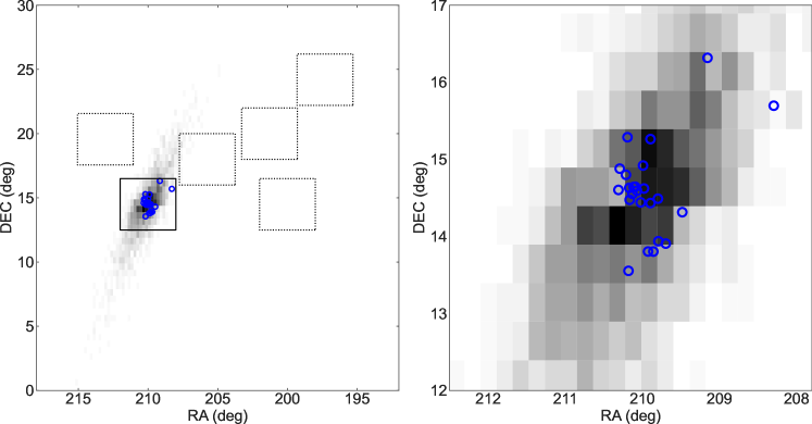
Figure 12: The predicted track of a mock stream generated by an idealized model of a satellite galaxy on the same orbit as Boo I in a fiducial Milky Way potential. The track is shown as a two-dimensional density histogram, where darker grey indicates higher density. It should be noted that the main body of the satellite is not plotted. The candidate BHB member stars of Boo I are shown as blue open circles, and the four-by-four degree footprints of the Boo I field and the off-fields are shown in solid and dotted lines, respectively, in the lefthand panel.

The candidate and confirmed member stars of Boo I presented in Longeard et al. (2021) form an elongated shape similar to that found in this present work, and those authors also explored tidal origins for this morphology using a very similar approach, and reached consistent conclusions.

Should, alternatively, Boo I not be tidally distorted from interacting with the Milky Way, the extended stellar envelope of Boo I must be produced in some other way. Possible alternative mechanisms for creating an extended stellar envelope invoke mergers or intense stellar feedback to provide the necessary energy injection. Simulations, such as those presented in Tarumi et al. (2021), show that it is certainly feasible to create an extended stellar distribution in a surviving UFD through an approximately equal-mass merger, after most of the star formation has occurred in the systems. The post-merger system in Tarumi et al. (2021) differs from Boo I – it is even more metal poor (mean $[\rm{Fe/H}]\sim-2.7$) and has a radial metallicity gradient that is steeper than that detected in Boo I (first tentatively discussed in Norris et al. 2010a, and recently confirmed in Longeard et al. 2021). The metallicity gradient in the simulations is enhanced by star formation, and thus chemical enrichment, in the inner regions during (and shortly after) the merger. Purely ‘dry’ mergers after star-formation has ceased could directly deposit stars in the outer regions, as found for one of the dwarf galaxies simulated by Rey et al. (2019). Placing constraints on the stellar age distribution, in addition to the chemical abundances, is of obvious importance to distinguish these scenarios.

4.1 Constraints on the Outer Envelope Stellar Population

The presence of nine candidate BHB member stars outside of the King profile nominal tidal radius of Boo I suggests that there should also be stars in redder phases of stellar evolution at similarly large projected distances. Indeed, as noted above, Norris et al. (2010a) and Longeard et al. (2021) identified luminous, evolved red stars with properties consistent with membership of Boo I far from its center. There should, of course, be many lower-luminosity stars and we estimated their possible contribution to the extended envelope by modeling a synthetic mono-age, mono-metallicity population with a standard IMF. Specifically, we generated a synthetic population from the PARSEC models (Bressan et al., 2012) in the PS1 photometry bands, using the web tool provided at http://stev.oapd.inaf.it/cgi-bin/cmd. We adopted a total stellar mass of $10^{5}\mathcal{M}_{\odot}$ (chosen purely for simplicity) with a Kroupa broken power-law IMF (Kroupa, 2001) and assumed a metallicity of $[\rm{M/H}]=-2.2$ (the lowest metallicity available) and an age of 13 Gyr. While not entirely representative of Boo I, this should provide a reasonable estimate for our present purposes.

We considered a ‘star’ in the synthetic population to be a BHB if it had a color $g_{PS1}-r_{PS1}\leq 0$ and it was in the core helium-burning phase of evolution, which resulted in 40 BHB ‘stars’. We then checked the number of luminous RGB stars by selecting all ‘stars’ on the first-ascent red giant branch that would be brighter than $g_{PS1}=20$ at the distance of Boo I, which yielded 44 (bright) RGB ‘stars’. This exercise thus predicts that there should be similar numbers of outer-envelope RGB as BHB, which is generally consistent with the findings of Norris et al. (2010a) and Longeard et al. (2021).

Looking ahead, for example to the Rubin Observatory, we considered all RGB, sub-giant, and main-sequence stars (hereafter ‘redder stars’) in the simulated population that would be brighter than $g_{PS1_{0}}=25$ if at the distance of Boo I (thus down to two magnitudes fainter than the MSTO). This predicts $\sim 135$ redder stars per BHB, and thus $9\times 135\sim 1,200$ redder stars (equivalent to $\sim 4,600\rm{L}_{\odot}$) in the extended stellar envelope. Assuming a uniform distribution over a (circular) annulus extending from the King profile nominal tidal radius to the projected radial distance of the furthest candidate member BHB star, i.e. from $\sim 0.7$ kpc to $\sim 2.3$ kpc, the resulting surface brightness of the (redder) stellar envelope would be $\mu\sim 35$ mag/square arcsec. Such a low-surface brightness envelope would be difficult to detect, but a suitably clumpy distribution could produce a more tractable over-density on the sky. Indeed, the furthest over-density from the center of Boo I detected by Roderick et al. (2016) is composed of stars fainter than $g\sim 22.75$. It may thus be possible for future work to leverage deep photometry and identify additional over-densities of redder stars beyond the King profile nominal tidal radius. Finally, we note that the number of candidate BHB member stars that we have identified beyond the areal coverage of earlier surveys implies that Boo I may have a higher total luminosity than previously estimated, a possibility that is also suggested by the relatively large number of associated RR Lyrae (Siegel, 2006).

5 Conclusion

This work explored the outer extents of the Boo I UFD, and revealed a stellar envelope of evolved blue stars that is more extended than previously thought. We investigated BHB and BSS stars as tracers of the stellar population of Boo I, as these blue stars occupy a distinct region in CMD-space that has relatively low contamination from either Milky Way stars and stellar remnants or extragalactic sources. We used a k-nearest neighbors classifier to identify likely BHB and BSS stars in Pan-STARRS griz photometry, as various color combinations of these filters has been shown to be sensitive to surface gravity in blue stars (see e.g. Vickers et al. 2012). We found twenty five BHB and four BSS within a $4\times 4$ degree field centered on Boo I  at appropriate apparent magnitudes to be members. We then cross-matched with Gaia EDR3, and determined that twenty-four of these twenty-five BHB have proper motions consistent with Boo I. None of the candidate member BSS stars has high-quality Gaia information and thus we could not quantify their proper motions. We then determined the expected contamination from non-member sources in the final sample of candidate Boo I members by repeating this selection process in various off-fields. From this exercise, we determined that the final Boo I candidate BHB member sample has a likely contamination level of $\lower 2.15277pt\hbox{$\;\buildrel<\over{\sim}\;$}10\%$.

Nine of the twenty-four candidate BHB member stars are at projected radii beyond the King profile nominal tidal radius derived by Muñoz et al. (2018), more than doubling the known population of member stars in these outer regions, including those of Longeard et al. (2021). These outer envelope stars confirm that Boo I has an extended spatial distribution, as indicated in e.g. Roderick et al. (2016). Their 2-dimensional morphology is evocative of that produced by tidal interactions. We explored this possibility by using the MockStreamGenerator within Gala to generate a mock stellar stream originating from an idealized satellite-galaxy progenitor, with properties similar to those inferred for Boo I. The candidate BHB member stars are, indeed, aligned with the resulting mock stream, indicating that tidal interactions are a plausible explanation for the observed morphology.

Candidate member stars at large distances from the center of their host galaxy, such as those identified here, present excellent targets for wide-field spectroscopic surveys. These stars present exciting opportunities to constrain the formation and evolution of their host systems. Wide-field spectroscopic instruments, such as the 2dF/AAOmage on the AAT and the Prime Focus Spectrograph on the Subaru telescope in Mauna Kea, will be able to observe stars over many square degrees in a small number of pointings, which will enable the exploration of the furthest extents of nearby dwarf and ultra-faint dwarf galaxies.

6 Acknowledgments

CF and RFGW acknowledge support through the generosity of Eric and Wendy Schmidt, by recommendation of the Schmidt Futures program. CF and RFGW thank the anonymous referee for their thorough report. RFGW thanks her sister, Katherine Barber, for her support of this research. CF and RFGW thank Imants Platais and Vera Kozhurina-Platais for insightful discussions.

The Pan-STARRS1 Surveys (PS1) and the PS1 public science archive have been made possible through contributions by the Institute for Astronomy, the University of Hawaii, the Pan-STARRS Project Office, the Max-Planck Society and its participating institutes, the Max Planck Institute for Astronomy, Heidelberg and the Max Planck Institute for Extraterrestrial Physics, Garching, The Johns Hopkins University, Durham University, the University of Edinburgh, the Queen’s University Belfast, the Harvard-Smithsonian Center for Astrophysics, the Las Cumbres Observatory Global Telescope Network Incorporated, the National Central University of Taiwan, the Space Telescope Science Institute, the National Aeronautics and Space Administration under Grant No. NNX08AR22G issued through the Planetary Science Division of the NASA Science Mission Directorate, the National Science Foundation Grant No. AST-1238877, the University of Maryland, Eotvos Lorand University (ELTE), the Los Alamos National Laboratory, and the Gordon and Betty Moore Foundation.

Funding for SDSS-III has been provided by the Alfred P. Sloan Foundation, the Participating Institutions, the National Science Foundation, and the U.S. Department of Energy Office of Science. The SDSS-III web site is http://www.sdss3.org/. SDSS-III is managed by the Astrophysical Research Consortium for the Participating Institutions of the SDSS-III Collaboration including the University of Arizona, the Brazilian Participation Group, Brookhaven National Laboratory, Carnegie Mellon University, University of Florida, the French Participation Group, the German Participation Group, Harvard University, the Instituto de Astrofisica de Canarias, the Michigan State/Notre Dame/JINA Participation Group, Johns Hopkins University, Lawrence Berkeley National Laboratory, Max Planck Institute for Astrophysics, Max Planck Institute for Extraterrestrial Physics, New Mexico State University, New York University, Ohio State University, Pennsylvania State University, University of Portsmouth, Princeton University, the Spanish Participation Group, University of Tokyo, University of Utah, Vanderbilt University, University of Virginia, University of Washington, and Yale University.

This work has made use of data from the European Space Agency (ESA) mission Gaia (https://www.cosmos.esa.int/gaia), processed by the Gaia Data Processing and Analysis Consortium (DPAC, https://www.cosmos.esa.int/web/gaia/dpac/consortium). Funding for the DPAC has been provided by national institutions, in particular the institutions participating in the Gaia Multilateral Agreement.

This work made use of data from the Guoshoujing Telescope (the Large Sky Area Multi-Object Fiber Spectroscopic Telescope LAMOST), a National Major Scientific Project built by the Chinese Academy of Sciences. Funding for the project has been provided by the National Development and Reform Commission. LAMOST is operated and managed by the National Astronomical Observatories, Chinese Academy of Sciences.

Appendix A Details of the Testing and Implementation of the KNN Classifier

The fractions of sources of the different types (BHB, BSS/MS, WD, and QSOs) in the SEGUE-PS1 catalog are not equal, which can bias the classifier (see e.g. Patel et al. 2020 for a discussion of the effect of class imbalance on KNN classification). There are, in total, 4995 BSS/MS stars, 2875 BHB stars, 475 WDs, and 280 QSOs with $-0.5\leq(g_{PS1}-r_{PS1})_{0}\leq 0$ in the catalog, so that more than half of the catalog is BSS/MS stars, while approximately a third is BHB stars. Class imbalance generally causes a classifier to be baised towards labelling objects as members of the majority class, which in our case is BSS stars. We mitigated this by resampling the SEGUE-PS1 data to create a balanced dataset for training and testing, as discussed below.

We opted to create a resampled catalog where each class (BSS/MS, BHB, WD, QSO) had approximately the same number of sources as do the BHBs in the original, SEGUE-PS1 catalog. This produced resampled catalogs containing $\sim 11,500$ sources. We under-sampled the BSS/MS class, i.e. we took a random subset of the stars in the BSS/MS class, while over-sampling the WD and QSO classes. We generated the required additional synthetic WD and QSO sources by first randomly selecting a WD or QSO source (with replacement) from the original SEGUE-PS1 catalog and then drawing griz magnitudes – to be assigned to the new synthetic source – from Gaussian distributions defined by the means and uncertainties of the PS1 photometry for the original source. We did explore another approach to over-sampling the QSO and WD samples (further discussed below), and opted to employ the approach just described, based on both its simplicity and the fact that it avoided the use of additional external data.

We used the KNeighborsClassifier module implemented in the scikit-learn Python package, adopting a Minkowski distance metric, and weighted the votes of each neighbor by the inverse of its distance from the input object such that closer training points have higher weight in deciding the label for the input object. We constructed two identically indexed arrays from the resampled SEGUE-PS1 catalog, such that every unique source had the same index in both arrays. One of the arrays contained every possible color combination of the PS1 colors for each source, while the other array contained the label for that source. We then randomly split these arrays into a training set, containing $70\%$ of the sample, and a test set, which contained the remaining $30\%$. We produced ten different resampled SEGUE-PS1 catalogs, each with its associated training and test sets, to reduce the dependence of the results on any one individual realization of the under-sampled BSS/MS stars or over-sampled WDs and QSOs.

We then determined the optimal k-value for the KNN classifier by training and testing it using a range of k-values between ${\rm k=1}$ and ${\rm k=100}$. We found that the completeness and purity of each class of source (as defined in Section 2.2 of the main text) varied with the different k-values, such that smaller k-values $(\leq 10)$ produced lower overall values for the completeness and purity. We found that k-values of around 20 produced samples of high completeness and purity for each class and the performance reached a plateau beyond that, motivating our choice of $k=20$.

With the optimal value of k identified, we then trained a KNN classifier on each of the training sets (i.e. we trained ten classifiers, each with the same parameters but different training data). We then applied the classifiers to the test sets and computed the completeness and purity of each output source type, or class. We also computed the confusion matrix for each pair of training set and test set, with an example shown in Table 3. Each row of the confusion matrix indicates the true class, and each column indicates the class that was assigned by the classifier. Thus entries on the diagonal of the matrix represent correctly labeled sources, while the off-diagonal entries represent mis-classifications. For example, the first row of the confusion matrix in Table 3 indicates that 728 BHB were correctly classified, 103 BHB were classified as BSS, 12 BHBs were classified as WDs, and 20 BHBs were classified as QSOs. The first column of the matrix in Table 3 indicates that 144 BSS were classified as BHB, 34 WDs were classified as BHB, and 4 QSO were classified as BHB. The last two rows give the overall purity and completeness for each class in this resampled SEGUE-PS1 catalog. The final purity and completeness for each class was obtained by averaging over all the resampled datasets and is reported in the first two rows of Table 4.

Table 3: Confusion Matrix

		BHB		BSS		WD		QSO
BHB		728		103		12		20
BSS		144		692		16		12
WD		34		79		732		12
QSO		4		19		25		805
Purity		80$\%$		77$\%$		93$\%$		95$\%$
Completeness		84$\%$		80$\%$		85$\%$		94$\%$

Note. — A representative confusion matrix for the KNN classifier resulting from training and testing on a random resampling of the SEGUE-PS1 catalog, as described in the text, with the training and test subsets containing, respectively, $70\%$ and $30\%$ of the sources. Each row in the table indicates the true label, and each column indicates the assigned label, such that the entries along the diagonal give the number of sources that were given correct labels, and off-diagonal entries show the number of mis-classifications into each other label. The purity and completeness of each type of source are given in the last two rows.

It is evident, from inspection of the confusion matrix, that it is rare for QSO sources to be mis-classified as either BHB or BSS/MS. This may have been anticipated, as QSOs are generally well-separated from the loci of BHB and BSS/MS in color-space (see e.g. Figure 3). The false-positive contribution of WDs to the BHB class is smaller than that of WDs to the BSS/MS class, which is perhaps unsurprising given that BHB stars have the lowest surface gravities out of the three and should thus be more well-separated from the highest surface gravity sources in color-space. The WD and QSO classes have the highest purity of the four classes, each with greater than $90\%$ purity, approximately $10\%$ higher than those of the BHB and BSS/MS classes.

We investigated how the performance of the classifier depended on the approach taken to over-sampling the WD and QSO classes. In this comparison, instead of producing synthetic WD and QSOs, we cross-matched external WD and QSO catalogs with the PS1 database and added a random subset of these additional sources to the SEGUE-PS1 catalog, again creating a dataset with equal sample sizes in each class of source and $\sim 11,500$ sources in total. We adopted the WD catalog of Gentile Fusillo et al. (2019) and considered only those sources sources that have both a high probability of being a white dwarf (Pwd $>.95$) and a small uncertainty in that probability (f_Pwd $<1$). We adopted the QSO catalog of Pâris et al. (2018). We employed the same matching and photometric quality criteria as described above for the SEGUE-PS1 catalog, and further required that the cross-matched sources have magnitudes within the $g_{PS1}$ magnitude range of the SEGUE-PS1 sample. We then randomly selected subsets of these data to add to the SEGUE-PS1 catalog, and again randomly under-sample the BSS class, and re-trained and re-tested the classifiers on ten random iterations of these new, augmented data.

Table 4: Average Purity and Completeness

		BHB		BSS		WD		QSO
Purity, Synthetic Sources		81$\%$		80$\%$		95$\%$		95$\%$
Completeness, Synthetic Sources		82$\%$		78$\%$		84$\%$		95$\%$
Purity, External Sources		81$\%$		78$\%$		94$\%$		95$\%$
Completeness, External Sources		82$\%$		76$\%$		84$\%$		95$\%$

Note. — The average purity and completeness of each class using the output of the classifiers trained on the a re-balanced catalog created with first synthetic WDs and QSOs (upper two rows) and second the addition of WDs and QSOs from external catalogs (lower two rows). In all cases, the probability threshold is $50\%$, i.e. sources must be assigned a given label with higher than $50\%$ probability in order to be classified as that type.

The resultant average purity and completeness of each class using the classifiers trained on these new data, created by including external catalogs, are given in the bottom two rows of Table 4. There is evidently little difference between the results obtained from either approach to rebalancing the different classes in the resampled SEGUE-PS1 catalog. As such, we proceeded with the first approach, in which we created synthetic sources.

We note, for completeness, that Smith et al. (2010) also investigated the use of a KNN classifier for the identification of BHB stars in broad-band photometric catalogs. However, their approach differs from that taken here in a few fundamental ways, which makes direct comparison of the classification results difficult. For example, Smith et al. (2010) use four color combinations of the SDSS ugri bands, and label sources in a binary fashion, simply as either BHB or not-BHB. Further, they use an equal ratio of BHB to not-BHB sources in the training set, but they adjust the output label probabilities with assumed priors. They do, however, provide the raw completeness, obtained before application of these priors, for the BHB class from their KNN classifier and their quoted value of $81.1\%$ is approximately the same as that found by our classifier.

Appendix B Dynamical Analysis

We derived the orbit of Boo I in two different Milky Way gravitational potentials (described below), which we use to set limits on the mass of Boo I. We adopt, as initial conditions for the orbit integrations, the mean line-of-sight velocity of Boo I given in Jenkins et al. (2020), the heliocentric distance estimate of Okamoto et al. (2012), and the mean proper motion we derived above. We performed a thousand Monte Carlo realizations of the orbit in each potential (assumed static), integrating each orbit over the time interval $-5$ Gyr to $+10$ Gyr. In each Monte Carlo realization, we drew the values of the component of proper motion ($\mu_{\alpha*}$, $\mu_{\delta}$), distance, and line-of-sight velocity from Gaussian distributions defined by the quoted means and errors of each parameter. The median and $16^{th}$ and $84^{th}$ percentiles of the resulting distribution of key orbital parameters for each adopted Milky Way potential are given in Table 5.

We first adopted the potential MWPotential2014, as implemented in galpy (described in detail in Bovy, 2015). The mass distribution corresponding to this potential has a virial mass of $0.8\times 10^{12}\mathcal{M}_{\odot}$ and is an idealized model consisting of a Navarro-Frenk-White (NFW) dark-matter halo (Navarro et al., 1996), a spherical bulge, and a Miyamoto-Nagai disk (Miyamoto & Nagai, 1975). For comparison, we also adopted the McMillan17 potential, again as implemented in galpy (described in detail in McMillan, 2017). The mass distribution of this second potential has a total virial mass of $1.3\times 10^{12}\mathcal{M}_{\odot}$, and is a more complex model fitted to the observational data, again assuming an NFW halo. As noted, in both cases, the Milky Way potential is static, and we neglected any contributions from other systems (such as the Large Magellanic Cloud).

Table 5: Derived Orbital Parameters

		MWPotential2014		McMillan17
Apocenter (kpc)		$105.36^{+22.27}_{-15.68}$		$89.03^{+13.65}_{-9.27}$
Pericenter (kpc)		$42.73^{+5.88}_{-6.71}$		$37.44^{+6.49}_{-5.85}$
Eccentricity		$0.43^{+0.02}_{-0.01}$		$0.41^{+0.02}_{-0.01}$

Note. — Median orbital parameters of Boo I, from 1000 Monte Carlo realizations of the initial conditions.

Under the assumption that all of the BHB candidate member stars are gravitationally bound to Boo I, their maximum radial distance from the center of Boo I (2.3 kpc in projection) can be used as a estimate of the tidal limit. We estimated the mass of Boo I in the two different Milky Way potentials using the rtide function within galpy (following Chiti et al., 2021). The rtide function assumes a point-mass potential for the satellite and that it is on a circular orbit. In the lower mass MWPotential2014 potential, a tidal radius of $r_{t}=2.3$ kpc requires that Boo I have a mass of $6.4\times 10^{7}\mathcal{M}_{\odot}$. In the higher mass McMillan17 potential, the same tidal radius requires that Boo I have a mass of $10.8\times 10^{7}\mathcal{M}_{\odot}$. For comparison, the King profile nominal tidal radius ($r_{t}=710$ pc) requires that Boo I have a mass of $0.2\times 10^{7}\mathcal{M}_{\odot}$ in the MWPotential2014 potential and $0.3\times 10^{7}\mathcal{M}_{\odot}$ in the McMillan17 potential, while the dynamical mass within the half-light radius has been estimated from the internal velocity dispersion to be $\sim 0.5\times 10^{7}\mathcal{M}_{\odot}$ (Jenkins et al., 2020).

Adopting, instead, the expression for the tidal radius of a (point mass) cluster on an elliptical orbit around a (point mass) galaxy from King (1962) (his Equation 11), gives very similar results. In this approximation, we estimated the mass interior to the orbit of Boo I in the MWPotential2014 model of the Milky Way using the mass_enclosed method within Gala, which assumes that the potential is spherical. Adopting the ellipticity from Table 5 and rearranging Equation 11 of King (1962), we find that a tidal radius of $r_{t}=2.3$ kpc requires that Boo I  have a mass of $22.2\times 10^{7}\mathcal{M}_{\odot}$. Adopting instead the King profile nominal tidal radius for Boo I from Muñoz et al. (2018), $r_{t}=710$ pc, would require Boo I to have a mass of $0.65\times 10^{7}\mathcal{M}_{\odot}$. The validity of the assumption that all stars are gravitationally bound to Boo I is yet unknown, but these exercises indicate that Boo I may be significantly more massive than estimated from data primarily within the central regions. We note that the higher values we obtained for the total mass, $\sim 10^{8}$ M_⊙, are entirely consistent with the virial masses of UFDs obtained by Nadler et al. (2020) from simulations of the Milky Way, together with its satellites.

Appendix C Additional, Sagittarius Stream Off-field

In this section we discuss an additional $4^{\circ}\times 4^{\circ}$ off-field, centered on (RA, Dec) = (200, 14.5), that we rejected due to the clear signal of the Sagittarius (Sgr) Stream. The proper motions of stellar sources in this field are shown in Figure 13; the prominent over-density at $(\mu_{\delta*},\mu_{\alpha})\sim(-1.1,-0.75)$ mas yr^-1 is most likely due to stars from the Sgr Stream. This field has a larger number of blue star-like sources (those with color $-0.5\leq(g_{PS1}-r_{PS1})_{0}\leq 0$) than any other field investigated in this work, with a total of 455 blue sources. We applied our KNN Classifier to these data and identified large numbers of both BHB and BSS stars (81 BHB and and 67 BSS in total). The enhanced presence of BHB and BSS, compared to the remaining fields, is consistent with the presence of the Sgr Stream. Further, only three of the identified BHB stars in this field have appropriate apparent magnitudes to be at the distance of Boo I. Following the procedure described in the main text, we cross-matched the PS1 catalog for this field with Gaia EDR3, and identified stars that have proper motions consistent with that of Boo I. Only one of the BHB stars at an appropriate apparent magnitude also has a proper motion that is consistent with that of Boo I. This low number is in agreement with the results reported above for the other off-fields. We can thus conclude that any possible contamination from the Sgr Stream in the Boo I candidate member BHB sample is minimal.

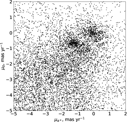
Figure 13: The Gaia EDR3 proper motions of sources in the rejected off-field. The over-density centered on $\mu_{\delta*}=\mu_{\alpha}=0$ is present in all fields used in this work, and is likely due to very distant sources, such as AGN and QSOs. The prominent over-density at $(\mu_{\delta*},\mu_{\alpha})\sim(-1.1,-0.75)$ mas yr^-1 is most likely due to stars in the Sagittarius Stream and is not present in the other fields.

References

- Astropy Collaboration et al. (2013) Astropy Collaboration, Robitaille, T. P., Tollerud, E. J., et al. 2013, A&A, 558, A33.
- Astropy Collaboration et al. (2018) Astropy Collaboration, Price-Whelan, A. M., Sipőcz, B. M., et al. 2018, AJ, 156, 123.
- Bailin (2019) Bailin, J. 2019, ApJS, 245, 5
- Baldwin et al. (2016) Baldwin, A. T., Watkins, L. L., van der Marel, R. P., et al. 2016, ApJ, 827, 12
- Battaglia et al. (2021) Battaglia, G., Taibi, S., Thomas, G. F., et al. 2021, arXiv:2106.08819
- Belokurov et al. (2006a) Belokurov, V., Zucker, D. B., Evans, N. W., et al. 2006, ApJ, 642, L137
- Belokurov et al. (2006b) Belokurov, V., Zucker, D. B., Evans, N. W., et al. 2006, ApJ, 647, L111
- Bernard et al. (2014) Bernard, E. J., Ferguson, A. M. N., Schlafly, E. F., et al. 2014, MNRAS, 442, 2999
- Bovill & Ricotti (2009) Bovill, M. S. & Ricotti, M. 2009, ApJ, 693, 1859
- Bovy (2015) Bovy, J. 2015, ApJS, 216, 29
- Bressan et al. (2012) Bressan, A., Marigo, P., Girardi, L., et al. 2012, MNRAS, 427, 127
- Brown et al. (2014) Brown, T. M., Tumlinson, J., Geha, M., et al. 2014, ApJ, 796, 91
- Bullock & Boylan-Kolchin (2017) Bullock, J. S. & Boylan-Kolchin, M. 2017, ARA&A, 55, 343
- Chambers et al. (2016) Chambers, K. C., Magnier, E. A., Metcalfe, N., et al. 2016, arXiv e-prints, arXiv:1612.05560.
- Chiti et al. (2021) Chiti, A., Frebel, A., Simon, J. D., et al. 2021, NatAs, 5, 392
- Clementini et al. (2019) Clementini, G., Ripepi, V., Molinaro, R., et al. 2019, A&A, 622, A60
- Cui et al. (2012) Cui, X.-Q., Zhao, Y.-H., Chu, Y.-Q., et al. 2012, RAA, 12, 1197
- Dall’Ora et al. (2006) Dall’Ora, M., Clementini, G., Kinemuchi, K., et al. 2006, ApJ, 653, L109
- Deason et al. (2018) Deason, A. J., Belokurov, V., & Koposov, S. E. 2018, ApJ, 852, 118
- Fardal et al. (2015) Fardal, M. A., Huang, S., & Weinberg, M. D. 2015, MNRAS, 452, 301.
- Farrow et al. (2014) Farrow, D. J., Cole, S., Metcalfe, N., et al. 2014, MNRAS, 437, 748
- Fellhauer et al. (2008) Fellhauer, M., Wilkinson, M. I., Evans, N. W., et al. 2008, MNRAS, 385, 1095.
- Fermani & Schönrich (2013) Fermani, F. & Schönrich, R. 2013, MNRAS, 430, 1294
- Flewelling et al. (2020) Flewelling, H. A., Magnier, E. A., Chambers, K. C., et al. 2020, ApJS, 251, 7
- Frebel et al. (2016) Frebel, A., Norris, J. E., Gilmore, G., et al. 2016, ApJ, 826, 110
- Fritz et al. (2018) Fritz, T. K., Battaglia, G., Pawlowski, M. S., et al. 2018, A&A, 619, A103
- Gaia Collaboration et al. (2018) Gaia Collaboration, Babusiaux, C., van Leeuwen, F., et al. 2018, A&A, 616, A10
- Gaia Collaboration et al. (2016) Gaia Collaboration, Prusti, T., de Bruijne, J. H. J., et al. 2016, A&A, 595, A1
- Gaia Collaboration et al. (2018) Gaia Collaboration, Helmi, A., van Leeuwen, F., et al. 2018, A&A, 616, A12
- Gaia Collaboration et al. (2020) Gaia Collaboration, Brown, A. G. A., Vallenari, A., et al. 2020, A&A, 649, A1
- Girardi et al (2005) Girardi L., Groenewegen M. A. T., Hatziminaoglou E. and da Costa L. 2005, A&A, 436, 895
- Geller et al. (2013) Geller, A. M., Hurley, J. R., & Mathieu, R. D. 2013, AJ, 145, 8
- Gentile Fusillo et al. (2019) Gentile Fusillo, N. P., Tremblay, P.-E., Gänsicke, B. T., et al. 2019, MNRAS, 482, 4570
- Goldman et al. (2019) Goldman, S. R., Boyer, M. L., McQuinn, K. B. W., et al. 2019, ApJ, 877, 49
- Gonneau et al. (2020) Gonneau, A., Lyubenova, M., Lançon, A., et al. 2020, A&A, 634, A133
- Green (2018) Green, G. M. 2018, The Journal of Open Source Software, 3, 695
- Hurley et al. (2005) Hurley, J. R., Pols, O. R., Aarseth, S. J., et al. 2005, MNRAS, 363, 293
- Jenkins et al. (2020) Jenkins, S., Li, T. S., Pace, A. B., et al. 2020, arXiv e-prints, arXiv:2101.00013
- King (1962) King I., 1962, AJ, 67, 471
- Koposov et al. (2011) Koposov, S. E., Gilmore, G., Walker, M. G., et al. 2011, ApJ, 736, 146
- Kroupa (2001) Kroupa, P., 2001, MNRAS, 322, 231
- Lancaster et al. (2019) Lancaster, L., Koposov, S. E., Belokurov, V., Evans, N. W., & Deason, A. J. 2019, MNRAS, 486, 378
- Lebzelter & Hinkle (2002) Lebzelter, T. & Hinkle, K. H. 2002, A&A, 393, 563
- Li et al. (2021) Li, H., Hammer, F., Babusiaux, C., et al. 2021, ApJ, 916, 8.
- Lindegren et al. (2018) Lindegren, L., Hernández, J., Bombrun, A., et al. 2018, A&A, 616, A2.
- Longeard et al. (2021) Longeard, N., Jablonka, P., Arentsen, A., et al. 2021, arXiv:2107.10849
- Nadler et al. (2020) Nadler, E. O., Wechsler, R. H., Bechtol, K., et al. 2020, ApJ, 893, 48
- Navarro et al. (1996) Navarro, J. F., Frenk, C. S., & White, S. D. M. 1996, ApJ, 462, 563
- Newell (1970) Newell, E. B. 1970, ApJ, 159, 443
- Nikolaev & Weinberg (2000) Nikolaev, S. & Weinberg, M. D. 2000, ApJ, 542, 804.
- Norris et al. (2008) Norris, J. E., Gilmore, G., Wyse, R. F. G., et al. 2008, ApJ, 689, L113
- Norris et al. (2010a) Norris, J. E., Gilmore, G., Wyse, R. F. G., et al. 2010, ApJ, 722, L104
- Norris et al. (2010b) Norris, J. E., Wyse, R. F. G., Gilmore, G., et al. 2010, ApJ, 723, 1632
- Okamoto et al. (2012) Okamoto, S., Arimoto, N., Yamada, Y., et al. 2012, ApJ, 744, 96
- Marconi et al. (2015) Marconi, M., Coppola, G., Bono, G., et al. 2015, ApJ, 808, 50
- Martin et al. (2007) Martin, N. F., Ibata, R. A., Chapman, S. C., et al. 2007, MNRAS, 380, 281
- Martínez-García et al. (2021) Martínez-García, A. M., del Pino, A., Aparicio, A., et al. 2021, MNRAS, 505, 5884
- McConnachie & Venn (2020) McConnachie, A. W., & Venn, K. A. 2020, AJ, 160, 124
- McDonald et al. (2010) McDonald, I., van Loon, J. T., Dupree, A. K., & Boyer M.L. 2010, MNRAS, 405, 1711
- McMillan (2017) McMillan, P. J. 2017, MNRAS, 465, 76
- Miyamoto & Nagai (1975) Miyamoto, M. & Nagai, R. 1975, PASJ, 27, 533
- Momany (2015) Momany, Y. 2015, in ‘Ecology of Blue Straggler Stars’, ed. H.M.J. Boffin, G. Carraro & G. Beccari, (Berlin, Heidelberg: Springer), ASSL, vol 413, p129
- Muñoz et al. (2006) Muñoz, R. R., Carlin, J. L., Frinchaboy, P. M., et al. 2006, ApJ, 650, L51
- Muñoz et al. (2018) Muñoz, R. R., Côté, P., Santana, F. A., et al. 2018, ApJ, 860, 66
- Pâris et al. (2018) Pâris, I., Petitjean, P., Aubourg, É., et al. 2018, A&A, 613, A51
- Patel et al. (2020) Patel, H., Rajput, D.S., Reddy, G.T., et al. 2020, International Journal of Distributed Sensor Networks, 16, 4
- Pedregosa et al. (2011) Pedregosa, F., Varoquaux, G., Gramfort, A., et al. 2011, Journal of Machine Learning Research, 12, 2825
- Plummer (1911) Plummer, H. C. 1911, MNRAS, 71, 460.
- Price-Whelan (2017) Price-Whelan, A. M. 2017, The Journal of Open Source Software, 2, 388.
- Read et al. (2006) Read, J. I., Wilkinson, M. I., Evans, N. W., et al. 2006, MNRAS, 366, 429.
- Rey et al. (2019) Rey, M. P., Pontzen, A., Agertz, O., et al. 2019, ApJ, 886, L3
- Roderick et al. (2016) Roderick, T. A., Mackey, A. D., Jerjen, H., et al. 2016, MNRAS, 461, 3702
- Salpeter (1955) Salpeter, E. E. 1955, ApJ, 121, 161.
- Santana et al. (2013) Santana, F. A., Muñoz, R. R., Geha, M., et al. 2013, ApJ, 774, 106
- Schlafly & Finkbeiner (2011) Schlafly, E. F., & Finkbeiner, D. P. 2011, ApJ, 737, 103
- Siegel (2006) Siegel, M. H. 2006, ApJ, 649, L83
- Simon (2019) Simon, J. D. 2019, ARA&A, 57, 375
- Sirko et al. (2004) Sirko, E., Goodman, J., Knapp, G. R., et al. 2004, AJ, 127, 899
- Smith et al. (2010) Smith, K. W., Bailer-Jones, C. A. L., Klement, R. J., et al. 2010, A&A, 522, A88
- Starkenburg et al. (2017) Starkenburg, E., Martin, N., Youakim, K., et al. 2017, MNRAS, 471, 2587.
- Starkenburg et al. (2019) Starkenburg, E., Youakim, K., Martin, N., et al. 2019, MNRAS, 490, 5757
- Tarumi et al. (2021) Tarumi, Y., Yoshida, N., & Frebel, A. 2021, ApJ, 914, L10.
- Taylor (2005) Taylor, M. B. 2005, in Astronomical Society of the Pacific Conference Series, Vol. 347, Astronomical Data Analysis Software and Systems XIV, ed. P. Shopbell, M. Britton, & R. Ebert, (San Francisco, CA: ASP), 29
- Tonry et al. (2012) Tonry, J. L., Stubbs, C. W., Lykke, K. R., et al. 2012, ApJ, 750, 99
- Vickers et al. (2012) Vickers, J. J., Grebel, E. K., & Huxor, A. P. 2012, AJ, 143, 86
- Vivas et al. (2020) Vivas, A. K., Martínez-Vázquez, C., Walker, A.R., 2020, ApJS, 247, 35
- Walsh et al. (2007) Walsh, S.M., Jerjen, H., & Willman, B. 2007, ApJ, 662, L83
- Walsh et al. (2008) Walsh, S.M., Willman, B., Sand, D., et al. 2008, ApJ, 688, 245
- Wilhelm et al. (1999) Wilhelm, R., Beers, T. C., & Gray, R. O. 1999, AJ, 117, 2308
- Xue et al. (2008) Xue, X. X., Rix, H. W., Zhao, G., et al. 2008, ApJ, 684, 1143
- Xue et al. (2011) Xue, X. X., Rix, H. W., Yanny, B., et al. 2011, ApJ, 738, 79
- Yanny et al. (2000) Yanny, B., Newberg, H. J., Kent, S., et al. 2000, ApJ, 540, 825
- Yanny et al. (2009) Yanny, B., Rockosi, C., Newberg, H. J., et al. 2009, AJ, 137, 4377
- Zhao et al. (2012) Zhao, G., Zhao, Y.-H., Chu, Y.-Q., et al. 2012, Research in Astronomy and Astrophysics, 12, 723.