Differentially Private Approximate Quantiles

Abstract

In this work we study the problem of differentially private (DP) quantiles, in which given dataset $X$ and quantiles $q_{1},...,q_{m}\in[0,1]$, we want to output $m$ quantile estimations which are as close as possible to the true quantiles and preserve DP. We describe a simple recursive DP algorithm, which we call ApproximateQuantiles (AQ), for this task. We give a worst case upper bound on its error, and show that its error is much lower than of previous implementations on several different datasets. Furthermore, it gets this low error while running time two orders of magnitude faster that the best previous implementation.

1 Introduction

Quantiles are the values that divide a sorted dataset in a certain proportion. They are one of the most basic and important data statistics, with various usages, ranging from computing the median to standardized test scores (GRE, 2021). Given sensitive data, publishing the quantiles can expose information about the individuals that are part of the dataset. For example, suppose that a company wants to publish the median of its users’ ages. Doing so means to reveal the date of birth of a certain user, thus compromising the user’s privacy. Differential privacy (DP) offers a solution to this problem by requiring the output distribution of the computation to be insensitive to the data of any single individual. This leads us to the definition of the DP-quantiles problem:

Definition 1.1 (The DP-Quantiles Problem).

Let $a,b\in\mathbb{R}$. Given a dataset $X\subseteq(a,b)$ containing $n$ points from $(a,b)$, and a set of $m$ quantiles $0<q_{1}\leq\dots\leq q_{m}<1$, privately identify quantile estimations $v_{1},...,v_{m}$ such that for every $j\in[m]$ we have $\Pr_{x\sim U_{X}}[x\leq v_{j}]\approx q_{j}$, where $U_{X}$ is the uniform distribution over the data $X$.

On the theory side, the DP-quantiles problem is relatively well-understood, with advanced constructions achieving very small asymptotic error (Beimel et al., 2016; Bun et al., 2015; Kaplan et al., 2020). However, as was recently observed by Gillenwater et al. (2021), due to the complexity of these advanced constructions and their large hidden constants, their practicality is questionable. This led Gillenwater et al. (2021) to design a simple algorithm for the DP-quantiles problem that performs well in practice. In this work we revisit the DP-quantiles problem. We build on the theoretical construction of Bun et al. (2015), and present a new (and simple) practical algorithm that obtains better utility and runtime than the state-of-the-art construction of Gillenwater et al. (2021) (and all other exiting implementations).

1.1 Our Contributions

We provide ApproximateQuantiles, an algorithm and implementation for the DP-quantiles problem (Section 3). We prove a worst case bound on the error of the AQ algorithm for arbitrary $m$ quantiles, and a tighter error bound for the case of uniform quantiles $q_{i}=i/(m+1)$, $i=1,\ldots,m$ (Section 3.2). We experimentally evaluated the AQ algorithm and conclude that it obtains higher accuracy and faster runtime than the existing state-of-the-art implementations (Section 4). In addition, we adapt our algorithm (and its competitors) to the definition of Concentrated Differential Privacy (zCDP) Bun and Steinke (2016). We show that its dominance over other methods is even more significant with this definition of privacy.

1.1.1 A Technical Overview of Our Construction: Algorithm ApproximateQuantiles

Our algorithm operates using a DP algorithm for estimating a single quantile. Specifically, we assume that we have a DP algorithm $\mathcal{A}:\mathbb{R}^{2}\times\mathbb{R}^{n}\times(0,1)\to\mathbb{R}$ that takes a domain $I=(a,b)\in\mathbb{R}^{2}$ (an interval on the line), a database $X\in\mathbb{R}^{n}$ (containing $n$ points in $I$), and a single quantile $q\in(0,1)$, and returns a point $v\in I$ such that $\Pr_{x\sim U_{X}}[x\leq v]\approx q$. Estimating a single quantile is a much easier task, with a very simple algorithm based on the exponential mechanism (McSherry and Talwar, 2007).

A naive approach of using $\mathcal{A}$ for solving the DP-quantiles problem would be to run it $m$ times (once for every given quantile). However, due to composition costs of running $m$ DP algorithms on the same data, the error with this approach would scale polynomially with $m$. As we demonstrate in our experimental results (in Section 4), this leads to a significantly reduced performance. In contrast, as we explain next, in our algorithm the error scales only logarithmically in the number of quantiles $m$.

The AQ algorithm privately estimates (using $\mathcal{A}$) the “middle quantile” $p=q_{\left\lceil m/2\right\rceil}$ and observes an answer $v$. Then it splits the problem into two sub-problems. The first sub-problem is defined over the dataset $X_{\ell}$ which contains the values from $X$ that are smaller than $v$. Its goal is to privately compute the quantiles $(q_{1},..,q_{\left\lceil m/2\right\rceil-1})/p$ on $X_{\ell}$. The second problem is defined over the dataset $X_{u}$ which contains the values from $X$ that are greater than $v$. The goal of the second problem is to privately compute $(q_{\left\lceil m/2\right\rceil+1}-p,\dots,q_{m}-p)/(1-p)$ on $X_{u}$. Notice that the recursive sub-problems have smaller ranges.

Specifically, at the first level of the recursion tree we compute one quantile $q_{1}^{1}\triangleq q_{\left\lceil m/2\right\rceil}$ on data points from a range $(a,b)$. We denote by $v_{1}^{1}$ the estimate which we receive. At the second level we compute two normalized quantiles $q_{2}^{1}\triangleq q_{\left\lceil m/4\right\rceil}/q_{1}^{1}$ and $q_{2}^{2}\triangleq q_{\left\lceil 3m/4\right\rceil}/(1-q_{1}^{1})$. The quantile $q_{2}^{1}$ is computed on data in the range $(a,v_{1}^{1})$, and we denote its estimate by $v_{2}^{1}$. The second quantile is computed on the data in the range $[v_{1}^{1},b]$, and we denote its estimate by $v_{2}^{1}$, and so on. Figure 1 illustrates this recursion tree.

Figure 1: The recursion tree of the algorithm. At each node we write the range of the corresponding subproblem and above it the part of the data in this subproblem.

[$(a,b)$ , name=root, label=${X=X_{1}^{1}}$ [$(a,v_{1}^{1})$, name=level1, label=$X_{2}^{1}$ [$(a,v_{2}^{1})$, name=level2, label=$X_{3}^{1}$ [$\vdots$]][$[v_{2}^{1},v_{1}^{1}]$,label=$X_{3}^{2}$ [$\vdots$]]] [$[v_{1}^{1},b]$, label=$X_{2}^{2}$ [$[v_{1}^{1},v_{2}^{2}]$,label=$X_{3}^{3}$[$\vdots$]][$[v_{2}^{2},b]$,label=$X_{3}^{4}$[$\vdots$]]]]

A few remarks are in order.

1. By shrinking the data range from one level to the next, we effectively reduce the error of algorithm $\mathcal{A}$ (because its error depends on the data range). We have found that, in practice, this has a large impact on our accuracy guarantees.

2. Note that every single data point participates only in $\log(m)+1$ sub-problems (one at each level). This allows our privacy loss (and, hence, our error) to grow only logarithmically in $m$.

1.2 Related Work

Private (Comulative Distribution Function) CDF estimation can be applied to estimating all the quantiles (Bun et al., 2015; Kaplan et al., 2020), however the theoretically best known algorithm for private CDF estimation (Bun et al., 2015) relies on several reductions, thus limiting its practicality. We present our AQ algorithm, inspired by Bun et al. (2015), taking their CDF estimation algorithm into practice. As opposed to the algorithm proposed by Bun et al. (2015), our algorithm avoids discretization of the domain by solving the DP single quantile problem using the exponential mechanism (Smith, 2011) instead of an interior point algorithm (Bun et al., 2015). Moreover, we split the data according the desired quantiles (rather than uniformly) while avoiding using the laplace mechanism in the process. A common tree-based approach to CDF estimation is included in our empirical error analysis (Section 4). A recent work by Gillenwater et al. (2021) proposed an instance of the exponential mechanism that simultaneously draws $m$ quantiles. The naive implementation of this exponential mechanism for $m$ quantiles is computationally difficult, but Gillenwater et al. (2021) provide a sophisticated $O(mn\log{n}+m^{2}n)$ implementation. The empirical experiments of Gillenwater et al. (2021) show that when the number of quantiles is small, $\mathrm{JointExp}$ algorithm preforms best. A comparison with this algorithm is included in our experiments (Section 4).

2 Preliminaries

A database $X$ is a set of $n$ points from some data domain $\mathcal{D}$. Differential privacy uses the definition of neighbors as follows.

Definition 2.1.

Databases $X$ and $X^{\prime}\in\mathcal{D}^{n}$ are neighbors, denoted $X\sim X^{\prime}$, if one of them can be obtained from the other by adding or removing a single element.

We use the add-remove definition of neighbors, as opposed to the swap definition (in which we replace a point instead of deleting or inserting it), although it is important to note that our algorithm ApproximateQuantiles (AQ) easily adapts to the swap framework.

Differential privacy can be defined using the notion of neighboring databases as follows:

Definition 2.2 (Dwork et al. (2006b)).

$\mathcal{A}$ randomized algorithm $\mathcal{A}\colon\mathcal{D}^{*}\to\mathcal{Y}$ is $(\varepsilon,\delta)$-differentially private ($(\varepsilon,\delta)$-DP) if, for every pair of neighboring databases $X,X^{\prime}$ and every output subset $Y\subseteq\mathcal{Y}$,

$$\Pr_{\mathcal{A}}[A(X)\in Y]\leq e^{\varepsilon}\cdot\Pr_{\mathcal{A}}[A(X^{\prime})\in Y]+\delta.$$

When $\delta>0$, we say $\mathcal{A}$ satisfies approximate differential privacy. If $\delta=0$, we say $\mathcal{A}$ satisfies pure differential privacy, and shorthand this as $\varepsilon$-differential privacy ($\varepsilon$-DP).

The composition property is a key benefit of differential privacy: an algorithm that relies on differentially private subroutines inherits an overall privacy guarantee by simply adding up the privacy guarantees of its components.

Lemma 2.3 (Dwork et al. (2006a, b)).

Let $\mathcal{A}_{1},\ldots,\mathcal{A}_{k}$ be $k$ algorithms that respectively satisfy $(\varepsilon_{1},\delta_{1})$-$,\ldots,(\varepsilon_{k},\delta_{k})$-differential privacy. Then running $\mathcal{A}_{1},\ldots,\mathcal{A}_{k}$ satisfies $\left(\sum_{i=1}^{k}\varepsilon_{i},\sum_{i=1}^{k}\delta_{i}\right)$-differential privacy.

The above lemma has come to be known as “basic composition” in the literature of differential privacy (see Dwork et al. (2010b) for more advanced composition theorems). Given Lemma 2.3, a simplistic approach for the DP-quantiles problem would be to estimate each of the $m$ quantiles separately, using an $\frac{\varepsilon}{m}$-DP algorithm, and then to apply Lemma 2.3 in order to show that the $m$ estimations together satisfy $\varepsilon$-DP. As we will see, our algorithm outperforms this simplistic approach by a large gap.

We will also rely on the exponential mechanism, a common building block for differentially private algorithms.

Definition 2.4 (McSherry and Talwar (2007)).

Given utility function $u\colon\mathcal{D}^{*}\times S\to\mathbb{R}$ mapping $(\text{database},\text{output})$ pairs to real-valued scores with $L_{1}$ sensitivity

$$\Delta_{u}\triangleq\max_{X\sim X^{\prime},s\in S}|u(X,s)-u(X^{\prime},s)|,$$

the probability that the exponential mechanism $M$ has an output $s\in S$ is:

$$\Pr[M(X)=s]\propto\exp\left(\frac{\varepsilon u(X,s)}{2\Delta_{u}}\right),$$

where $\propto$ elides the normalization factor.

The exponential mechanism maintains the database’s privacy while prioritizing its higher utility outputs.

Lemma 2.5 (McSherry and Talwar (2007)).

The mechanism described in Definition 2.4 is $\varepsilon$-DP and for error parameter $\gamma>0$ satisfies that:

$$\Pr_{s\in S}[u(X,s)>\mathrm{Opt}-\gamma]\leq|S|\cdot\exp\left(-\frac{\varepsilon\gamma}{2\Delta}\right),$$

where $\mathrm{Opt}=\max_{s\in S}\{u(X,s)\}$.

In our case in this paper, the solution space $S$ is infinite. Specifically, it is an interval $(a,b)$. Lemma A.1 in Appendix A adapts the exponential mechanism to this setting.

3 ApproximateQuantiles Algorithm

This section demonstrates our differentially private quantiles algorithm, ApproximateQuantiles. As we mentioned in the introduction, our algorithm uses a subroutine $\mathcal{A}$ for privately estimating a single quantile. We implement algorithm $\mathcal{A}$ using the exponential mechanism (see Appendix A). We remark that, if the dataset is given sorted, then $\mathcal{A}$ runs in linear time, and the time required for all recursive calls at the same level of the recursion tree is $O(n)$. It follows that the overall time complexity of AQ algorithm is $O(n\log{m})$.

Algorithm 1 - ApproximateQuantiles (AQ) Differentially Private Quantiles

Input: Domain $\mathcal{D}=(a,b)$, database $X=(x_{1},\dots,x_{n})\in\mathcal{D}^{n}$, quantiles $Q=(q_{1},\dots,q_{m})$, privacy parameter $\varepsilon$.

1:Let $\mathcal{A}:\mathbb{R}^{2}\times\mathbb{R}^{n}\times(0,1)\to\mathbb{R}$ be a $\frac{\varepsilon}{\log{m}+1}$-DP mechanism for a single quantile.

2:function F($(a,b),X,Q$)

3:     if $m=0$ then return $null$

4:     else if $m=1$ then

5:         return $\{\mathcal{A}((a,b),X,q_{1})\}$      

6:     Let $\hat{m}=\left\lceil m/2\right\rceil$

7:     Let $p=q_{\hat{m}}$

8:     Let $v=\mathcal{A}((a,b),X,p)$

9:     Let $X_{\ell},X_{u}=\{x\in X\mid x<v\},\{x\in X\mid x>v\}$

10:     Let $Q_{\ell}=(q_{1},\dots,q_{\hat{m}-1})/p$

11:     Let $Q_{u}=(q_{\hat{m}+1}-p,\dots,q_{m}-p)/(1-p)$

12:     return $\textsc{F}((a,v),X_{\ell},Q_{\ell})\cup\{v\}\cup\textsc{F}((v,b),X_{u},Q_{u})$

We denote by $q_{i}^{j}$ the normalized quantile computed by the $j$th subproblem at the $i$th level of the algorithm’s recursion tree, and by $v_{i}^{j}$ the result of this computation. Note that the number of subproblems at level $i$ is $2^{i-1}$. (At the last level some of the subproblems may be empty.) We let $X_{i}^{j}$ be the data used to compute $v_{i}^{j}$. It was created by splitting the data $X_{i-1}^{\left\lceil j/2\right\rceil}$ into two parts according to $v_{i-1}^{\left\lceil j/2\right\rceil}$. We note that $X_{i}^{j_{1}}$ and $X_{i}^{j_{2}}$ are disjoint for a fixed level $i$ and $j_{1}\not=j_{2}$. This allows us to avoid splitting our privacy budget between subproblems at the same level of the recursion, and we split it only between different levels, see Section 3.1. We also denote $Q_{i}\triangleq(q_{i}^{1},\dots,q_{i}^{2^{i-1}})$ and $V_{i}\triangleq(v_{i}^{1},\dots,v_{i}^{2^{i-1}})$.

We assume that the data does not contain duplicate points. This can be enforced by adding small perturbations to the points. The answer we return is with respect to the perturbed points. In fact the utility of our algorithm depends on the minimum distance between a pair of points.

3.1 Privacy Analysis

First we prove that AQ algorithm is $\varepsilon$-DP.

Lemma 3.1 (Differential Privacy).

If $\cal A$ is an $\frac{\varepsilon}{\log{m}+1}$-DP mechanism for a single quantile then AQ algorithmis $\varepsilon$-DP.

Proof.

It suffices to show that for each level $1\leq i\leq\log{m}+1$ the output $V_{i}$ is $\frac{\varepsilon}{\log{m}+1}$-DP, since the number of levels is $\log{m}+1$, from composition (Lemma 2.3) we get that the AQ algorithm satisfies $(\varepsilon,\delta)$-DP.

Let $X$ and $X^{\prime}=X\cup\{x^{\prime}\}$ be neighboring databases, mark as ${X^{\prime}}_{i}^{k}$ the part of level $i$ that contains $x^{\prime}$ among ${X^{\prime}}_{i}^{j}$, $1\leq j\leq 2^{i-1}$ (as explained above, only one ${X^{\prime}}_{i}^{j}$ contains $x^{\prime}$). For each $j\neq k$ the data $X_{i}^{j}$ equals ${X^{\prime}}_{i}^{j}$ and therefore the probability of the output $v_{i}^{j}$ is the same under $X$ or $X^{\prime}$. The output $v_{i}^{k}$ is obtained by $\mathcal{A}$ which is a $\frac{\varepsilon}{\log{m}+1}$-DP mechanism, therefore it satisfies $\frac{\varepsilon}{\log{m}+1}$-DP.

∎

3.2 Utility Analysis

A $q_{i}$-quantile is any point $o_{i}\in(a,b)$ such that the number points of $X$ which are in $(a,o_{i})$ is $\lfloor q_{i}n\rfloor$. We also define the gap, $\mathrm{Gap}_{X}(d_{1},d_{2})$, between $d_{1},d_{2}\in(a,b)$ with respect to $X$ are the number of points in the data $X$ that fall between $d_{1}$ and $d_{2}$, formally:

$$\mathrm{Gap}_{X}(d_{1},d_{2})=|\{x\in X\mid x\in[\min\{d_{1},d_{2}\},\max\{d_{1},d_{2}\})\}|.$$

Using this notion we define the error of the algorithm. Given dataset $X$, quantiles $Q=(q_{1},\dots,q_{m})$, solution $V=(v_{1},\dots,v_{m})$ and true quantiles $O=(o_{1},\dots,o_{m})$, the maximum missed points error is defined as:

$$\mathrm{Err}_{X}(O,V)=\max_{j\in[m]}\{\mathrm{Gap}(o_{j},v_{j})\}=\max_{j\in[m]}\{||\{x\in X|x<v_{j}\}|-\lfloor q_{j}\cdot n\rfloor|\}.$$

This error was first defined by Smith (2011) and is widely used in the literature on the differentially private quantiles problem. We first analyze the error of our algorithm in the general case, without any constraints on the given quantiles.

Lemma 3.2 (General Quantiles Utility).

Let $X\in(a,b)^{n}$ be a database, and let $\mathcal{A}$ be an algorithm that computes an approximation $v$ for a single quantile $q$ of $X$ such that

$$\Pr[\mathrm{Gap}_{X}(o,v)>\gamma]\leq\frac{\beta}{m}.$$

for some constants $\beta,\gamma>0$, where $o$ is a true $q$-quantile. We run AQ algorithm using $\mathcal{A}$ on a database $X$, and quantiles $Q=(q_{1},\dots,q_{m})$. Then, with probability $1-\beta$, we get approximate quantiles $V=(v_{1},\dots,v_{m})$ such that $\mathrm{Err}_{X}(O,V)\leq(\log{m}+1)\gamma$.

Proof.

For the computation of $m$ quantiles the AQ algorithm applies $\mathcal{A}$ at most $m$ times (once per each internal node of the recursion tree). Since in each run $\mathcal{A}$ has error at most $\gamma$ with probability $1-\beta/m$ it follows by a union bound that:

$$\Pr[\exists i,j\text{ s.t.\ }\mathrm{Gap}_{X}(\hat{o}_{i}^{j},v_{i}^{j})>\gamma]\leq\beta,$$ (1)

where $\hat{o}_{i}^{j}$ is a true $q_{i}^{j}$-quantile with respect to the dataset $X_{i}^{j}$. We also denote by $o_{i}^{j}$ a true $q_{k}$-quantile with respect to $X$ where $q_{k}$ is the original fraction in $Q$ that corresponds to $q_{i}^{j}$ (see Figure 2).

At the first level $(i=1)$ of the recursive tree we compute one quantile $q_{1}^{1}$ on the data $X=X_{1}^{1}$ and therefore $\mathrm{Gap}_{X}(\hat{o}_{1}^{1},o_{1}^{1})=0$. At the second leval $(i=2)$, we split the data $X$ according to $v_{1}^{1}$ into $X_{2}^{1},X_{2}^{2}$, since $\mathrm{Gap}_{X}(v_{1}^{1},o_{1}^{1})\leq\gamma$, the $q_{2}^{j}$-quantile $\hat{o}_{2}^{j}$ of the dataset $X_{2}^{j}$ satisfies that $\mathrm{Gap}_{X}(\hat{o}_{2}^{j},o_{2}^{j})\leq\gamma$ (see Figure 2). By induction, at layer $i$, for every $j$ we have that $\mathrm{Gap}_{X}(\hat{o}_{i}^{j},o_{i}^{j})\leq(i-1)\cdot\gamma$. Combining this with Equation (1) results in $\mathrm{Gap}_{X}(v_{i}^{j},o_{i}^{j})\leq i\cdot\gamma$. At the last level $(i=\log{m}+1)$ we have that $\mathrm{Gap}_{X}(v_{i}^{j},o_{i}^{j})\leq(\log{m}+1)\cdot\gamma$. ∎

Theorem 3.3.

Assume that we implement $\mathcal{A}$ using the exponential mechanism with privacy parameter $\frac{\varepsilon}{\log{m}+1}$, as described in Appendix A to solve the single quantile problem. Then, given a database $X\in(a,b)^{n}$ and quantiles $Q=(q_{1},\dots,q_{m})$ the AQ algorithm is $\varepsilon$-DP, and with probability $1-\beta$ output $V=(v_{1},\dots,v_{m})$ that satisfies

$$\mathrm{Err}_{X}(O,V)\leq 2(\log{m}+1)\cdot\frac{\log{\psi}+\log{m}-\log{\beta}}{\varepsilon}=O\left(\frac{\log{m}(\log{\psi}+\log m+\log{\frac{1}{\beta}})}{\varepsilon}\right),$$

where $\psi=\frac{b-a}{\min_{k\in[n+1]}\{x_{k}-x_{k-1}\}}$.

Proof.

By Lemma A.1, the exponential mechanism with privacy parameter $\frac{\varepsilon}{\log{m}+1}$ has an error more than $2\frac{\log{\psi}+\log{m}-\log{\beta}}{\varepsilon}$ with probability at most $\frac{\beta}{m}$. Therefore, by Lemma 3.2, the AQ algorithm has an error no larger than $\gamma=2(\log{m}+1)\cdot\frac{\log{\psi}+\log{m}-\log{\beta}}{\varepsilon}$ with probability $1-\beta$. Combining this with Lemma 3.1 the theorem follows. ∎

Figure 2: An error in computing $v_{1}^{1}$ by at most $\gamma=2$ points from the optimal value $o_{1}^{1}$, might cause an error of at most $\gamma$ points between the value of $o_{j}^{2}$ compared to $\hat{o}_{j}^{2}$. The example demonstrates the computed quantiles $q_{1}=\frac{1}{4}$, $q_{2}=\frac{1}{2}$ and $q_{3}=\frac{3}{4}$. Note that $q_{2}^{1}$, $q_{2}^{2}=\frac{1}{2}$.

The uniform quantiles problem is a common instance of the quantiles problem where $q_{i}=\frac{i}{m+1}$, for $i=1,\ldots,m$. Lemma 3.4 shows that when the desired quantiles are uniform it is possible to guarantee that $\mathrm{Err}_{X}(O,V)=O(\gamma)$ with probability $1-\beta$.

Lemma 3.4 (Uniform Quantiles Utility).

Let $X\in(a,b)^{n}$ be a database, and let $\mathcal{A}$ be an algorithm that computes an approximation $v$ for a single quantile $q$ of $X$ such that

$$\Pr[\mathrm{Gap}_{X}(o,v)>\gamma]\leq\frac{\beta}{m}.$$

for some constants $\beta,\gamma>0$, where $o$ is a true $q$-quantile. We run AQ algorithm using $\mathcal{A}$ on a database $X$, and quantiles $Q=(q_{1},\dots,q_{m})$ where $q_{i}=\frac{i}{m+1}$. Then, with probability $1-\beta$, the AQ algorithm returns approximate quantiles $V=(v_{1},\dots,v_{m})$ satisfying $\mathrm{Err}_{X}(O,V)\leq 2\gamma$.

Proof.

For simplicity we assume that $m=2^{k}-1$. The proof is similar for other values of $m$. For this value of $m$ we have that $q_{\ell}=\ell/2^{k}$, $\ell=1,\ldots,2^{k}-1$ and $q_{i}^{j}=1/2$ for all $i$ and $j$. Furthermore, we have that the number of points in $X\cap(a,o_{i}^{j})$ is $\lfloor\frac{2\cdot j-1}{2^{i}}n\rfloor$, $j=1,\ldots,2^{i-1}$.

As in Lemma 3.2, Equation (1) holds. So we assume in the rest of the proof that $\mathrm{Gap}_{X}(v_{i}^{j},\hat{o}_{i}^{j})\leq\gamma$ for all $i$ and $j$.

For the root $(i=1)$ of the recursion tree we compute one quantile $q_{1}^{1}$ on the data $X=X_{1}^{1}$ and therefore $\mathrm{Gap}_{X}(\hat{o}_{1}^{1},o_{1}^{1})=0$. At the second level, $(i=2)$, we split the data $X$ according to $v_{1}^{1}$ into $X_{2}^{1}$, and $X_{2}^{2}$. Since $\mathrm{Gap}_{X}(v_{1}^{1},o_{1}^{1})\leq\gamma$, we have that $\lfloor n/2\rfloor-\gamma\leq|X_{2}^{j}|\leq\lfloor n/2\rfloor+\gamma$. Recall that $|X\cap(a,o_{2}^{1})|=\lfloor n/4\rfloor$ and $|X\cap(a,o_{2}^{2})|=\lfloor 3n/4\rfloor$ and therefore $\mathrm{Gap}_{X}(\hat{o}_{2}^{j},o_{2}^{j})\leq\gamma/2$ for $j=1,2$. Now, since $\mathrm{Gap}_{X}(v_{2}^{j},\hat{o}_{2}^{j})\leq\gamma$ we get that $\lfloor n/4\rfloor-3\gamma/2\leq|X_{3}^{j}|\leq\lfloor n/4\rfloor+3\gamma/2$, and therefore $\mathrm{Gap}_{X}(\hat{o}_{3}^{j},o_{3}^{j})\leq 3\gamma/4$, for $j\in[4]$. Similarly, since $\mathrm{Gap}_{X}(v_{3}^{j},\hat{o}_{3}^{j})\leq\gamma$, it follows that $\lfloor n/8\rfloor-7\gamma/4\leq|X_{4}^{j}|\leq\lfloor n/8\rfloor+7\gamma/4$ and therefore $\mathrm{Gap}_{X}(\hat{o}_{4}^{j},o_{4}^{j})\leq 7\gamma/8$, for $j\in[8]$. We conclude that by induction on the levels we get that,

$$\mathrm{Gap}_{X}(\hat{o}_{i}^{j},o_{i}^{j})\leq\frac{2^{i-1}-1}{2^{i-1}}\cdot\gamma\leq\gamma,$$

for all $i$ and $j$. Combining this upper bound with Equation (1) we get that $\mathrm{Gap}_{X}(v_{j}^{i},o_{j}^{i})\leq 2\gamma$. ∎

Theorem 3.5 improves the bound of Theorem 3.6 for uniform quantiles. We omit its proof which is similar to the proof of Theorem 3.6 using Lemma 3.4 instead of Lemma 3.2.

Theorem 3.5.

If we set $\mathcal{A}$ to be the exponential mechanism with privacy parameter $\frac{\varepsilon}{\log{m}+1}$, as described in Appendix A, then given data $X\in(a,b)^{n}$ and quantiles $Q=(q_{1},\dots,q_{m})$, where $q_{i}=\frac{i}{m+1}$, the AQ algorithm is $\varepsilon$-DP and with probability $1-\beta$ output $V=(v_{1},\dots,v_{m})$ that satisfies

$$\mathrm{Err}_{X}(O,V)=O\left(\frac{\log{\psi}+\log m+\log{\frac{1}{\beta}}}{\varepsilon}\right),$$

where $\psi=\frac{b-a}{\min_{k\in[n+1]}\{x_{k}-x_{k-1}\}}$.

Quantiles sanitization.

Given a database $X=(x_{1},..,x_{n})\in(a,b)^{n}$, we can produce a differentially private dataset $\hat{X}=(\hat{x}_{1},\dots,\hat{x}_{n})\in(a,b)^{n}$, such that for each point $\hat{x}_{\ell}$, the number of points in $\hat{X}$ that are smaller than $\hat{x}_{\ell}$ is similar to the number of points in $X$ that are smaller than $\hat{x}_{\ell}$. This is specified precisely in the following Corollary of Theorem 3.6. In particular this corollary implies that for every interval $I\subseteq(a,b)$, $|X\cap I|$ is approximately equal to $|\hat{X}\cap I|$.

Corollary 3.6.

Assume that we implement $\mathcal{A}$ using the exponential mechanism with privacy parameter $\frac{\varepsilon}{\log n+1}$, as described in Appendix A, to solve the single quantile problem. Then, given a database $X\in(a,b)^{n}$ and $n$ quantiles $Q=(q_{1},\dots,q_{n})$, where $q_{i}=i/n$, the AQ algorithm is $\varepsilon$-DP, and with probability $1-\beta$ output $\hat{X}=(\hat{x}_{1},\dots,\hat{x}_{n})$ that satisfies

$$\mathrm{Err}_{X}(X,\hat{X})=O\left(\frac{\log{n}(\log{\psi}+\log n+\log{\frac{1}{\beta}})}{\varepsilon}\right).$$

where $\psi=\frac{b-a}{\min_{k\in[n+1]}\{x_{k}-x_{k-1}\}}$.

3.3 Zero-Concentrated Differential Privacy

Zero Concentrated Differential Privacy (zCDP) (Bun and Steinke, 2016) offers smoother composition properties than standard $(\varepsilon,\delta)$-DP. The general idea is to to compare the Rényi divergence of the privacy losses random variables for neighboring databases. We analyse our algorithm also under this definition of privacy. As in Section 3.1, the privacy analysis of our algorithm applies composition of the processing of different levels in the recursion tree. zCDP’s composition theorem allows us to run the exponential mechanism at each level with a higher privacy parameter, which results in a tighter error bound for the exponential mechanism. For precise statements see Theorem 3.10 and Theorem 3.11 below. In Section 4.3 we measure empirically the benefit the gain from this smoother composition of zCDP.

Definition 3.7 (Zero-Concentrated Differential Privacy (zCDP) Bun and Steinke (2016)).

An algorithm $M:\mathcal{D}^{n}\to\mathbb{R}$ is $\rho$-zCDP if for all neighbouring $X,X^{\prime}\in\mathcal{D}^{n}$, and $\gamma\in(1,\infty)$ $\mathrm{RD}_{\gamma}(M(Z),M(Z^{\prime}))\leq\rho\gamma$, where $\mathrm{RD}_{\gamma}$ is the $\gamma$-Rényi divergence between random variables A and B. ($\cal D$ is the domain of the database elements, in our case it is $(a,b)$.)

Lemma 3.8.

(Bun and Steinke, 2016) if algorithm $M$ satisfies $\varepsilon$-DP, then $M$ satisfies $\rho$-zCDP with $\rho=\frac{\varepsilon^{2}}{2}$.

Lemma 3.9.

(Bun and Steinke, 2016) Let $M:\mathcal{D}^{n}\to\mathcal{Y}$ and $M^{\prime}:\mathcal{D}^{n}\to\mathcal{Z}$. suppose $M$ satisfies $\rho$-zCDP and $M^{\prime}$ satisfies $\rho^{\prime}$-zCDP. Define $M^{\prime\prime}:\mathcal{D}^{n}\to\mathcal{Z}$ by $M^{\prime\prime}(X)=M^{\prime}(X,M(X))$. Then $M^{\prime\prime}$ satisfies $(\rho+\rho^{\prime})$-zCDP.

Theorem 3.10 (General Quantiles Utility with zCDP).

Suppose we implement $\mathcal{A}$ using the exponential mechanism to solve the single quantile problem, with privacy parameter $\varepsilon=\sqrt{\frac{2\rho}{\log{m}+1}}$. Then, given data $X$ and quantiles $Q=(q_{1},\dots,q_{m})$, the AQ algorithm is $\rho$-zCDP and with probability $1-\beta$ output $V=(v_{1},\dots,v_{m})$ that satisfies

$$\mathrm{Err}_{X}(O,V)\leq 2(\log{m}+1)\sqrt{\frac{\log{m}+1}{2\rho}}\cdot(\log{\psi}+\log{m}-\log{\beta})=O\left(\frac{\log^{1.5}{m}}{\sqrt{\rho}}(\log{\psi}+\log{m}+\log{\frac{1}{\beta}})\right),$$

where $\psi=\frac{b-a}{\min_{k\in[n+1]}\{x_{k}-x_{k-1}\}}$.

Proof.

By Lemma 3.1, the computation at each recursive level $1\leq i\leq\log{m}+1$ is $\sqrt{\frac{2\rho}{\log{m}+1}}$-DP, and therefore, by Lemma 3.8, also $(\frac{\rho}{\log{m}+1})$-zCDP. Since the number of levels is $\log{m}+1$, by Lemma 3.9, the AQ algorithm is $\rho$-zCDP. The error bound follows exactly as in the proof of Theorem 3.6. ∎

The following theorem is analogous to Theorem 3.5. Its privacy proof is as for Theorem 3.10 and the error analysis is as in the proof of Theorem 3.5.

Theorem 3.11 (Uniform Quantiles Utility with zCDP).

Suppose we implement $\mathcal{A}$ using the exponential mechanism to solve the single quantile problem, with privacy parameter $\sqrt{\frac{2\rho}{\log{m}+1}}$. Then, given data $X$ and quantiles $Q=(q_{1},\dots,q_{m})$, where $q_{i}=\frac{i}{m+1}$, the AQ algorithm is $\rho$-zCDP, and with probability $1-\beta$ output $V=(v_{1},\dots,v_{m})$ that satisfies

$$\mathrm{Err}_{X}(O,V)=O\left(\sqrt{\frac{\log{m}}{\rho}}(\log{\psi}+\log{m}+\log{\frac{1}{\beta}})\right),$$

where $\psi=\frac{b-a}{\min_{k\in[n+1]}\{x_{k}-x_{k-1}\}}$.

4 Experiments

We implemented the AQ algorithm in Python and its code is publicly available on GitHub. We used the exponential mechanism for the DP single quantile algorithm $\mathcal{A}$, with $-\mathrm{Gap}_{X}(o,v)$ as the utility of a solution $v$, where $o$ is a true quantile, see Appendix A. We also experimented with the AQ-zCDP algorithm, a version of our algorithm that is private with respect to the definition of zero-concentrated differential privacy (zCDP) (Section 3.3). We compared our algorithms to the three best performing algorithms from Gillenwater et al. (2021) called: (1) JointExp (2) $\mathrm{AppindExp}$ and (3) AggTree. We ran the implementations provided by Gillenwater et al. (2021). We describe these baseline algorithms in Section 4.1. We tested the algorithms using two synthetic datasets and four real datasets that are described in Section 4.2. For each dataset we compared the accuracy (Section 4.3) and runtime (Section 4.4) of the competing algorithms.

4.1 Baseline Algorithms

JointExp (Gillenwater et al., 2021) solves the DP quantiles problem by an efficient implementation of the exponential mechanism (Definition 2.4) on $m$-tuples $V=(v_{1},\dots,v_{m})\in(a,b)^{m}$, where the utility of $V$ is defined as follows:

$$u(X,V)=-\sum_{j\in[m+1]}|\mathrm{Gap}_{X}(o_{j},o_{j-1})-\mathrm{Gap}_{X}(v_{j},v_{j-1})\}|,$$

where we define $v_{0}=o_{0}=a$ and $v_{m+1}=o_{m+1}=b$. The naive implementation of the exponential mechanism with this utility function is computationally difficult: The number of $m$ tuples $V$ is infinite, and there may even be exponentially many (in $m$) equivalence classes of such $m$-tuples. Gillenwater et al. (2021) give an $O(mn\log{n}+m^{2}n)$ time algorithm to sample from the distribution defined by the exponential mechanism. The experiments of Gillenwater et al. (2021) show that when the number of quantiles, $m$, is small the $\mathrm{JointExp}$ algorithm preforms best.

AppindExp solves the DP quantiles problem by applying the exponential mechanism as described in Appendix A to find every quantile $q_{i}$ separately. Since $\mathrm{AppindExp}$ applies the exponential mechanism $m$ times, if we use $\varepsilon/m$ as the privacy parameter for each application of the exponential mechanism, then by composition we get that $\mathrm{AppindExp}$ is $\varepsilon$-DP.

The advanced composition theorem Dwork et al. (2010b) shows that if we use $\varepsilon^{\prime}\approx\varepsilon/\sqrt{m\log(1/\delta)}$ for each application of the exponential mechanism then the overall algorithm would be $(\varepsilon,\delta)$-DP. The implementation of Gillenwater et al. (2021) uses a tighter advanced composition theorem specific for nonadaptive applications of the exponential mechanism (Dong et al., 2020), to determine an $\varepsilon^{\prime}$ for each quatile computation such that the overall composition of the $m$ applications is $(\varepsilon,\delta)$-DP. We use $n=1000$ data points in our experiments, so we chose $\delta=10^{-6}$ in accordance with the common practice that $\delta\ll\frac{1}{n}$.

AggTree Dwork et al. (2010a) and Chan et al. (2011) implement an $\varepsilon$-DP tree-based counting algorithm for CDF estimation. Given a domain $(a,b)$ the algorithm builds a balanced tree $T$ with branching factor $b$ and height $h$, so $T$ has $b^{h}$ leaves. The $j$’th leaf of the tree is associated with sub-domain $[c_{j-1},c_{j}]$ where $c_{j}:=a+j(b-a)/b^{h}$. Given a dataset $D\in(a,b)^{n}$, the algorithm starts by counting the number of elements from the dataset that fall into each leaf (i.e. are contained in its sub-domain). Each internal node of $T$ is associated with the sum of the counters of its children (which equals to the number of elements in the leaves of its subtree). In particular, the count associated with the root is $n$. Since each element in the data contributes to at most $h$ nodes (the path from the leaf containing it to the root), it suffice to add $\mathrm{Lap}(h/\varepsilon)$ noise to the value of each node to make the counts of $T$ $\epsilon$-DP.

We can approximate any quantile $q$ using this data structure as follows. We find the leftmost leaf $z$ such that the sum of the noisy counts of all leaves to the left of $z$ (including $z$) is at least $q\cdot n$. In particular, if the counts were not noisy that $z$ would contain a $q$th quantile. Let $c(z)$ be the noisy count of $z$ and let $c^{-}(z)$ be the sum of the noisy counts of the leaves to the left of $z$. Let $p=(qn-c^{-}(z))/c(z)$. Without noise $p$ would have been the approximate relative quantile of the $q$th quantile among the elements in $z$. Let $[c_{k-1},c_{k}]$ be the range associated with $z$. We approxmate the $q$th quantile using linear interpolation inside $[c_{k-1},c_{k}]$. That is we return $(1-p)c_{k-1}+pc_{k}$. We utilize the $\mathrm{AggTree}$ implementation provided by Gillenwater et al. (2021), and the results are given in Section 4.3.

4.2 Datasets

We tested our four algorithms on six datasets. Two data sets are synthetic. One contains independent samples from the uniform distribution $U(-5,5)$, and the other contains independent samples from the Gaussian $N(0,5)$. Two real continuous datasets from Goodreads (2019), one contains book ratings and the other contains books’ page counts. Last we have two categorial datasets from the adults’ census data (Dua and Graff, 2019). One contains working hours per week and the other ages of different persons. Table 4.2 shows the properties of each dataset, and Figure 4.2 shows the histograms of 100 equal-width bins for each dataset.

Figure 3: Histograms of 100 equal-width bins.

Data set	Size	Data Characteristics
Uniform (synthetic)	10000	Continuous
Gaussian (synthetic)	10000	Continuous
Goodreads rating	11123	Continuous
Goodreads pages	11123	Continuous
Adult hours	48842	96 Categories
Adult age	48842	74 Categories

Table 1: Data set properties.

4.3 Empirical Error Analysis

We compare the error of ApproximateQuantiles and the baseline algorithms. Our error metric is the average gap of the approximate quantiles $V=(v_{1},\ldots,v_{m})$ and and the true ones $O=(o_{1},\ldots,o_{m})$:

$$\frac{\sum_{j\in[m]}\mathrm{Gap}_{X}(o_{j},v_{j})}{m}\ .$$

DP Error Analysis:

We randomly chose $1000$ samples from each dataset and checked the error of each algorithm with $m=1$ to $m=120$ uniform quantiles in the range $[-100,100]$. We used the privacy parameter $\varepsilon=1$. This process was repeated $100$ times. Figure 4 shows the average of the error across the $100$ iterations. Figure 5 zooms in on the error for $m=1,\ldots,35$ quantiles. ApproximateQuantiles performs better than the baselines almost in all experiments, except for a few small values of $m$ where the performance of $\mathrm{JointExp}$ was slightly better. As the number of quantiles increases ApproximateQuantiles wins by a larger margin.

zCDP Error Analysis:

As in previous experiments we randomly chose $1000$ samples from each dataset and checked the error of each algorithm for $m=1,\ldots,120$ uniform quantiles in the range $[-100,100]$. All algorithms were $\rho$-zCDP for $\rho=\frac{1}{2}$. For this we used $\varepsilon^{\prime}=1/\sqrt{m}$ in each application of the exponential mechanism by $\mathrm{AppindExp}$, and a Laplace noise of magnitude $\varepsilon^{\prime}=\sqrt{h}$ in each node of the tree computed by $\mathrm{AggTree}$. In each application of the exponential mechanism by ApproximateQuantiles we used $\varepsilon^{\prime}=\sqrt{1/(\log m+1)}$ as described in Theorem 3.11. The algorithm JointExp with $\varepsilon=1$ is $\frac{1}{2}$-zCDP by Lemma 3.9, so its error is the same as in the previous experiment. Figure 6 shows the average of the error for z-CDP across the $100$ iterations. Figure 7 zooms in on the error for $m=1,\ldots,35$. ApproximateQuantiles performs much better than the baselines even for small number of quantiles.

Figure 4: The $x-$axis shows the number of quantiles and the $y-$axis shows the gap per quantile averaged over 100 trials with $\varepsilon=1$. Note that the graphs are in log scale.

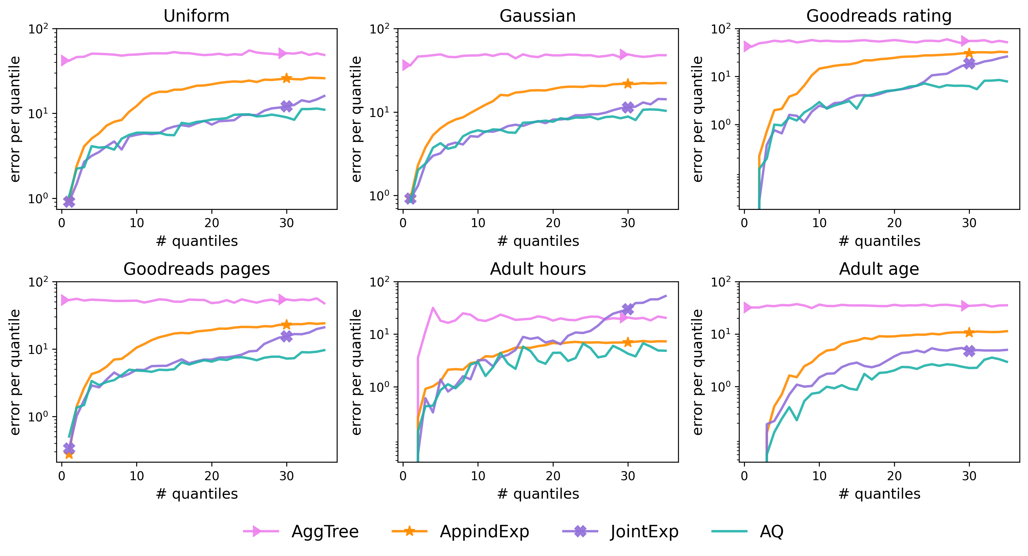
Figure 5: The $x-$axis shows the number of quantiles and the $y-$axis shows the gap per quantile averaged over 100 trials with $\varepsilon=1$. Note that the graphs are in log scale.

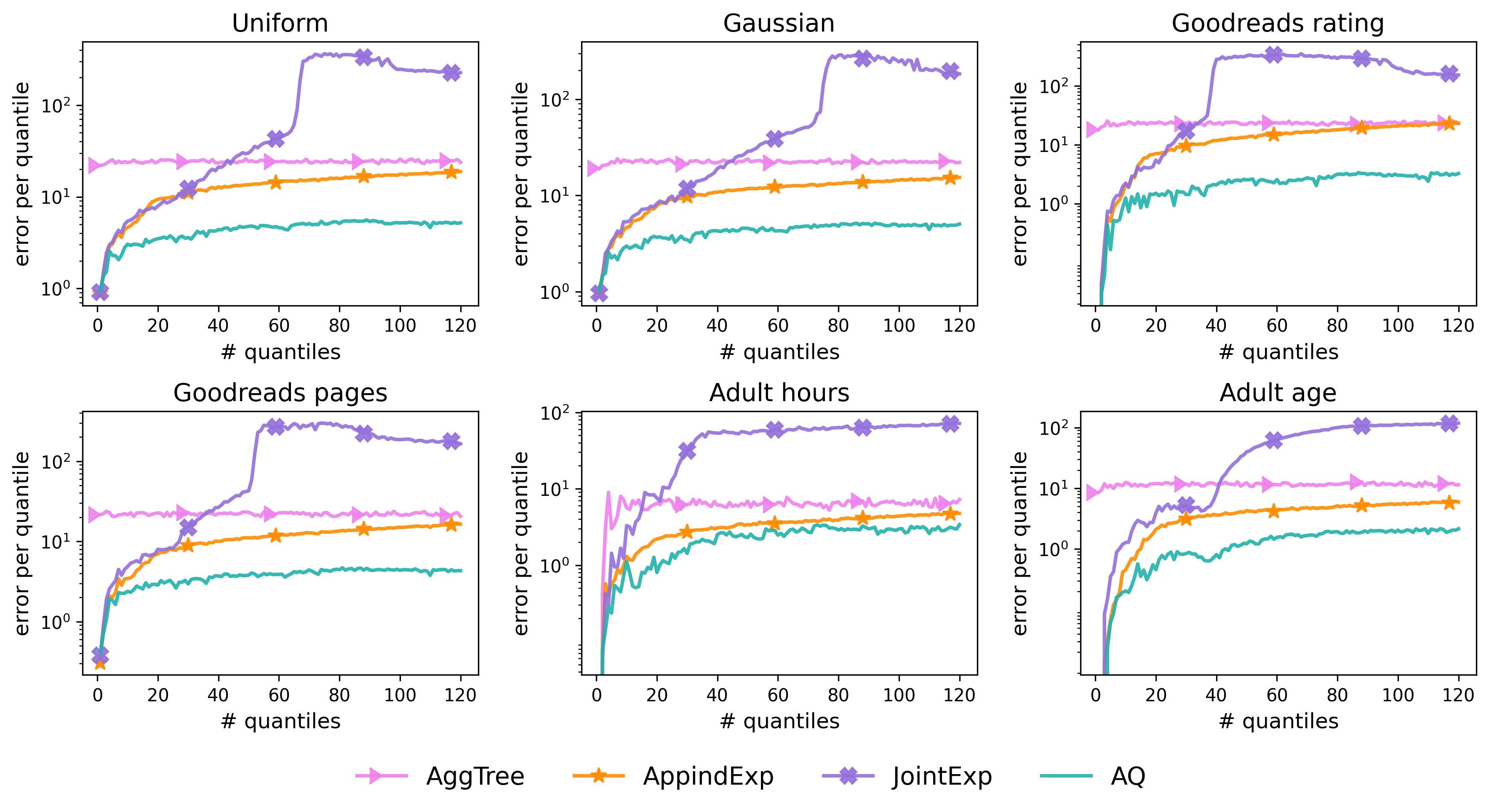
Figure 6: zCDP: The $x-$axis shows the number of quantiles and the $y-$axis shows the gap per quantile averaged over 100 trials with $\rho=1/2$. Note that the graphs are in log scale.

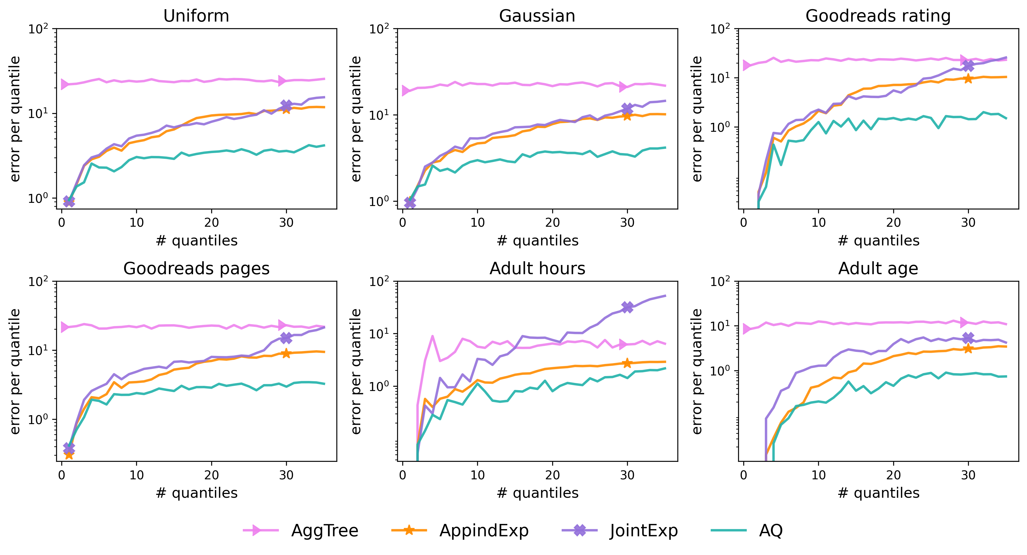
Figure 7: zCDP: The $x-$axis shows the number of quantiles and the $y-$axis shows the gap per quantile averaged over 100 trials with $\rho=1/2$. Note that the graphs are in log scale.

4.4 Time Complexity Experiments

Given a sorted dataset, it takes $O(n)$ time to find all quantiles at a single level of the recursion tree of ApproximateQuantiles. Therefore the overall time complexity (i.e., without the sort) of the AQ algorithm is $O(n\log{m})$, where $m$ is the number of quantiles. In comparison, the baseline algorithms are computationally more expensive: $\mathrm{JointExp}$ algorithm runs in $O(mn\log{n}+m^{2}n)$ time, $\mathrm{AppindExp}$ algorithm runs in $O(mn)$ time and $\mathrm{AggTree}$ algorithm runs in $O(n\log{n})$ time. We empirically compared the running time of ApproximateQuantiles to the running times of the baseline algorithms. For each dataset we measured the time required to find $m\in[120]$ quantiles in a sub-sample of size $1000$ of each dataset, averaged over $100$ trials per dataset. Figure 8 shows the average running time across all datasets (Section 4.2), each experiment used one core of an Intel i9-9900K processor. We see that the running time of ApproximateQuantiles  is about ten times smaller than of $\mathrm{AggTree}$ and at least a $100$ smaller than of $\mathrm{JointExp}$ and $\mathrm{AppindExp}$ .

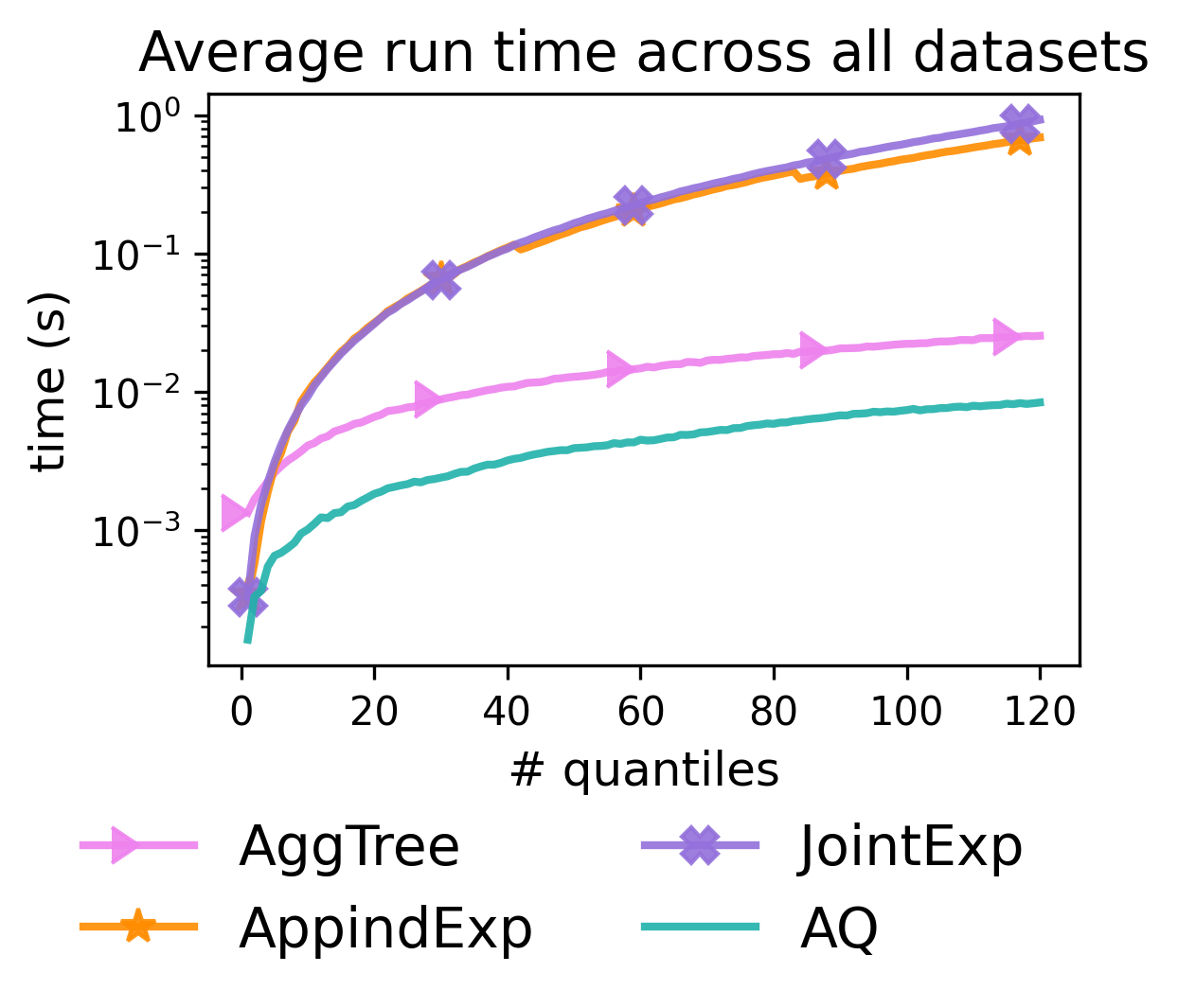
Figure 8: $x-$axis number of quantiles, $y-$axis is the run time averaged across all datasets, each dataset averaged across $100$ trials. Note that the graphs are in log scale.

Appendix

Appendix A DP Single quantile

In the DP single quantile problem, the input is a single quantile $q$ and a database $X\in(a,b)^{n}$. The output is a quantile estimate $v\in(a,b)$ such that $\Pr_{x\sim U_{X}}[x\leq v]\approx q$ (in a sense that Lemma A.1 would make precise). We solve this problem using the exponential mechanism of McSherry and Talwar [2007] on $(a,b)$ with the utility function:

$$u(X,w)=-\left||\{x\in X|x<w\}|-\lfloor q\cdot n\rfloor\right|=-\mathrm{Gap}_{X}(o,w),$$

where $o$ is a $q$-quantile and $w\in(a,b)$. This mechanism samples each point $w\in(a,b)$ to be the output with density proportional to $\exp(\varepsilon u(X,w)/2)$. Note that the sensitivity of $u$ is $1$, that is $\max\{|u(X,\omega)-u(X^{\prime},\omega)|\}\leq 1$, where the maximum is over neighboring datasets $X$ and $X^{\prime}$ and points $\omega\in(a,b)$. The largest utility is of a $q$-quantile and equals to $0$.

We can sample from this distribution using the technique given by Smith [2011] (see their Algorithm 2). The idea is to split the sampling process into two steps:

1. Let $I_{k}=[x_{k-1},x_{k}]]$, $k=1,\ldots,n+1$ where $x_{0}=a$, $x_{n+1}=b$, be the set of $n+1$ intervals between data points. We sample an interval from this set of intervals, where the probability of sampling $I_{k}$ is proportional to

   $$\Pr[\mathcal{A}(X)=I_{k}]\propto\exp\left(\frac{\varepsilon u(X,I_{k})}{2}\right)\cdot(x_{k}-x_{k-1}),$$

   Note that all points in $I_{k}$ have the same utility which we denote by $u(X,I_{k})$.

2. Return a uniform random point from the sampled interval.

Lemma A.1.

Given dataset $X\in(a,b)^{n}$ and quantile $q\in[0,1]$, the exponential mechanism is $\varepsilon$-DP, and with probability $1-\beta$ outputs $v$ that satisfies

$$\mathrm{Gap}_{X}(o,v)\leq 2\cdot\frac{\log{\psi}-\log{\beta}}{\varepsilon},$$

where $o$ is a true $q$-quantile and $\psi=\frac{b-a}{\min_{k\in[n+1]}\{x_{k}-x_{k-1}\}}$.

Proof.

$\varepsilon$-DP follows in a straightforward way by bounding the ratio of the densities of a point $w$ in the destribution defined by $X$ and in the distribution defined by $X^{\prime}$; See also Dwork and Roth [2014].

Let $I_{t}$ be an interval such that $u(X,I_{t})\leq-\gamma$. It follows that the probability of sampling a point from $I_{t}$ is at most

$$\Pr[\mathcal{A}(X)=I_{t}]\leq\frac{\exp\left(\frac{-\varepsilon\gamma}{2}\right)\cdot(x_{t}-x_{t-1})}{\sum_{k\in[n+1]}\exp\left(\frac{\varepsilon u(X,I_{k})}{2}\right)\cdot(x_{k}-x_{k-1})}\ .$$

Using the union bound we get that:

$$\Pr[\mathcal{A}(X)\leq-\gamma] \leq \frac{\exp\left(\frac{-\varepsilon\gamma}{2}\right)(b-a)}{\sum_{k\in[n+1]}\exp\left(\frac{\varepsilon u(X,I_{k})}{2}\right)\cdot(x_{k}-x_{k-1})}$$

$$\leq \frac{\exp\left(\frac{-\varepsilon\gamma}{2}\right)(b-a)}{\exp\left(\frac{\varepsilon u(X,I_{o})}{2}\right)(x_{o}-x_{o-1})}$$

$$\leq \frac{b-a}{\min_{k\in[n+1]}(x_{k}-x_{k-1})}\cdot\exp\left(\frac{-\varepsilon\gamma}{2}\right)$$

$$= \psi\exp\left(\frac{-\varepsilon\gamma}{2}\right)$$

where $I_{o}$ is the interval containing the $q$-quantiles so $u(X,I_{0})=0$. It follows that with probability less than $\beta$, we sample an interval whose utility is at most $-\gamma$ for

$$\gamma=2\Delta_{u}\cdot\frac{\log{\psi}-\log{\beta}}{\varepsilon}.$$

Since in the second step we sample the $q$-quantile $v$ uniformly from the interval selected in the first step, we get that with probability $1-\beta$ the output $v$ satisfies:

$$\mathrm{Gap}_{X}(o,v)\leq 2\cdot\frac{\log{\psi}-\log{\beta}}{\varepsilon}.$$

∎

References

- Beimel et al. [2016] Amos Beimel, Kobbi Nissim, and Uri Stemmer. Private learning and sanitization: Pure vs. approximate differential privacy. Theory Comput., 12(1):1–61, 2016.
- Bun and Steinke [2016] Mark Bun and Thomas Steinke. Concentrated differential privacy: Simplifications, extensions, and lower bounds. In Theory of Cryptography Conference, pages 635–658. Springer, 2016.
- Bun et al. [2015] Mark Bun, Kobbi Nissim, Uri Stemmer, and Salil Vadhan. Differentially private release and learning of threshold functions. In 2015 IEEE 56th Annual Symposium on Foundations of Computer Science, pages 634–649. IEEE, 2015.
- Chan et al. [2011] T-H Hubert Chan, Elaine Shi, and Dawn Song. Private and continual release of statistics. ACM Transactions on Information and System Security (TISSEC), 14(3):1–24, 2011.
- Dong et al. [2020] Jinshuo Dong, David Durfee, and Ryan Rogers. Optimal differential privacy composition for exponential mechanisms. In International Conference on Machine Learning, pages 2597–2606. PMLR, 2020.
- Dua and Graff [2019] Dheeru Dua and Casey Graff. UCI machine learning repository, 2019. URL http://archive.ics.uci.edu/ml. Date accessed: 2021-07-01.
- Dwork and Roth [2014] Cynthia Dwork and Aaron Roth. The algorithmic foundations of differential privacy. Foundations and Trends in Theoretical Computer Science, 9(3-4):211–407, 2014.
- Dwork et al. [2006a] Cynthia Dwork, Krishnaram Kenthapadi, Frank McSherry, Ilya Mironov, and Moni Naor. Our data, ourselves: Privacy via distributed noise generation. In EUROCRYPT, volume 4004 of Lecture Notes in Computer Science, pages 486–503. Springer, 2006a.
- Dwork et al. [2006b] Cynthia Dwork, Frank McSherry, Kobbi Nissim, and Adam Smith. Calibrating noise to sensitivity in private data analysis. In Theory of cryptography conference, pages 265–284. Springer, 2006b.
- Dwork et al. [2010a] Cynthia Dwork, Moni Naor, Toniann Pitassi, and Guy N Rothblum. Differential privacy under continual observation. In Proceedings of the forty-second ACM symposium on Theory of computing, pages 715–724, 2010a.
- Dwork et al. [2010b] Cynthia Dwork, Guy N. Rothblum, and Salil Vadhan. Boosting and differential privacy. In 2010 IEEE 51st Annual Symposium on Foundations of Computer Science, pages 51–60, 2010b.
- Gillenwater et al. [2021] Jennifer Gillenwater, Matthew Joseph, and Alex Kulesza. Differentially private quantiles. In ICML, volume 139 of Proceedings of Machine Learning Research, pages 3713–3722. PMLR, 2021.
- Goodreads [2019] Goodreads. Goodreads-books dataset, 2019. URL https://www.kaggle.com/jealousleopard/. Date accessed: 2021-07-01.
- GRE [2021] GRE. Ets. gre guide to the use of scores., 2021. URL https://www.ets.org/s/gre/pdf/gre_guide.pdf. Date accessed: 2021-07-19.
- Kaplan et al. [2020] Haim Kaplan, Katrina Ligett, Yishay Mansour, Moni Naor, and Uri Stemmer. Privately learning thresholds: Closing the exponential gap. In Conference on Learning Theory, pages 2263–2285. PMLR, 2020.
- McSherry and Talwar [2007] Frank McSherry and Kunal Talwar. Mechanism design via differential privacy. In 48th Annual IEEE Symposium on Foundations of Computer Science (FOCS’07), pages 94–103. IEEE, 2007.
- Smith [2011] Adam Smith. Privacy-preserving statistical estimation with optimal convergence rates. In Proceedings of the forty-third annual ACM symposium on Theory of computing, pages 813–822, 2011.