The One Step Malliavin scheme: new discretization of BSDEs implemented with deep learning regressions

Abstract

A novel discretization is presented for forward-backward stochastic differential equations (FBSDE) with differentiable coefficients, simultaneously solving the BSDE and its Malliavin sensitivity problem. The control process is estimated by the corresponding linear BSDE driving the trajectories of the Malliavin derivatives of the solution pair, which implies the need to provide accurate $\Gamma$ estimates. The approximation is based on a merged formulation given by the Feynman-Kac formulae and the Malliavin chain rule. The continuous time dynamics is discretized with a theta-scheme. In order to allow for an efficient numerical solution of the arising semi-discrete conditional expectations in possibly high-dimensions, it is fundamental that the chosen approach admits to differentiable estimates. Two fully-implementable schemes are considered: the BCOS method as a reference in the one-dimensional framework and neural network Monte Carlo regressions in case of high-dimensional problems, similarly to the recently emerging class of Deep BSDE methods [23, 27]. An error analysis is carried out to show $\mathds{L}^{2}$ convergence of order $1/2$, under standard Lipschitz assumptions and additive noise in the forward diffusion. Numerical experiments are provided for a range of different semi- and quasi-linear equations up to $50$ dimensions, demonstrating that the proposed scheme yields a significant improvement in the control estimations.

Keywords: backward stochastic differential equations, Malliavin calculus, Deep BSDE, neural networks, BCOS, gamma estimates

1 Introduction

In this paper, we are concerned with the numerical solution of a system of forward-backward stochastic differential equations (FBSDE) where the randomness in the backward equation (BSDE) is driven by a forward stochastic differential equation (SDE). These systems are written in the general form

$$X_{t} =x_{0}+\int_{0}^{t}\mu(s,X_{s})\mathrm{d}s+\int_{0}^{t}\sigma(s,X_{s})\mathrm{d}W_{s},$$ (1.1a)

$$Y_{t} =g(X_{T})+\int_{t}^{T}f(s,X_{s},Y_{s},Z_{s})\mathrm{d}s-\int_{t}^{T}Z_{s}\mathrm{d}W_{s},$$ (1.1b)

where $\{W_{t}\}_{0\leq t\leq T}$ is a $d$-dimensional Brownian motion and $\mu:[0,T]\times\mathds{R}^{d\times 1}\to\mathds{R}^{d\times 1}$, $\sigma:[0,T]\times\mathds{R}^{d\times 1}\to\mathds{R}^{d\times d}$, $g:\mathds{R}^{d\times 1}\to\mathds{R}^{q}$ and $f:[0,T]\times\mathds{R}^{d\times 1}\times\mathds{R}^{q}\times\mathds{R}^{q\times d}\to\mathds{R}^{q}$ are all deterministic mappings of time and space, with some fixed $T>0$. Adhering to the stochastic control terminology, we often refer to $Z$ as the control process. We shall work under the standard well-posedness assumptions of Pardoux and Peng [38], which require Lipschitz continuity of the corresponding coefficients in order to ensure the existence of a unique solution pair $\{(Y_{t},Z_{t})\}_{0\leq t\leq T}$ adapted to the augmented natural filtration. The main motivation to study FBSDE systems lies in their connection with parabolic, second-order partial differential equations (PDE), generalizing the well-known Feynman-Kac relations to non-linear settings. Indeed, considering the quasi-linear, parabolic terminal problem

$$\begin{split}\partial_{t}u(t,x)+\frac{1}{2}\Tr{\sigma\sigma^{T}(t,x){\text{Hess}_{x}u}(t,x)}+\innerproduct{\mu(t,x)}{\nabla_{x}u(t,x)}+f(t,x,u,\nabla_{x}u(t,x)\sigma(t,x))&=0\\ u(T,x)&=g(x),\end{split}$$ (1.2)

the Markov solution to Equation 1.1 coincides with the solution of Equation 1.2 in an almost sure sense, provided by the non-linear Feynman-Kac relations

$$Y_{t}=u(t,X_{t}),\qquad Z_{t}=\nabla_{x}u(t,X_{t})\sigma(t,X_{t}).$$ (1.3)

Consequently, the BSDE formulation provides a stochastic representation to the simultaneous solution of a parabolic problem and its gradient, which is an advantageous feature for several applications in stochastic control and finance, where sensitivities play a fundamental role. These relations can be extended to viscosity solutions in case Equation 1.2 does not admit to a classical solution – see [38]. Moreover, it is known – see [38, 14, 26, 35] – that under suitable regularity assumptions the solution pair of the backward equation is differentiable in the Malliavin sense [37], and the Malliavin derivatives $\{(D_{s}Y_{t},D_{s}Z_{t})\}_{0\leq s,t\leq T}$ satisfy a linear BSDE themselves, where the $Z$ process admits to a continuous modification provided by $Z_{t}=D_{t}Y_{t}$.

From a numerical standpoint, the main challenge in solving BSDEs stems from the approximation of conditional expectations. Indeed, a discretization of the backward equation in Equation 1.1b yields a sequence of recursively nested conditional expectations at each point in the discretized time window. Over the years, several methods have been proposed to tackle the solution of the FBSDE system using: PDE methods in [33]; forward Picard iterations in [5]; quantization techniques in [3]; chaos expansion formulas in [8]; Fourier cosine expansions in [40, 41] and regression Monte Carlo approaches in [21, 7, 6]. These methods have shown great results in low-dimensional settings, however, the majority of them suffers from the curse of dimensionality, meaning that their computational complexity scales exponentially in the number of dimensions. Although, regression Monte Carlo methods have been successfully proven to overcome this burden, they are difficult to apply beyond $d=10$ dimensions due to the necessity of a finite regression basis. The primary challenge in the numerical solution of BSDEs is related to the approximation of the $Z$ process. In particular, the standard backward Euler discretization results in a conditional expectation estimate of $Z$ which scales inverse proportionally with the step size of the time discretization – see [7]. This phenomenon poses a significant amount of difficulty in least-squares Monte Carlo frameworks, as the corresponding regression targets have diverging conditional variances in the continuous limit.

Recently, the field has received renewed attention due to the pioneering paper of Han et al. [23], in which they reformulate the backward discretization in a forward fashion, parametrize the control process of the solution by deep neural networks and train the resulting sequence of networks in a global optimization given by the terminal condition of Equation 1.1b. Their method has enjoyed various modifications and extensions, see, e.g., [17, 4]. In particular, Huré et al. in [27] proposed an alternative where the optimization of the sequence of neural networks is done in a backward recursive manner, similarly to classical regression Monte Carlo approaches. We refer to the class of these deep learning based formulations as Deep BSDE methods. Although such Deep BSDE solvers have shown remarkable empirical results in solving high-dimensional problems, they struggle to solve the whole FBSDE system in Equation 1.1b and are merely focused on the PDE problem. In particular, the approach of [23] solely captures the solution pair at $t=0$; whereas the extension of [27] gives good approximations at future time steps, its accuracy in the $Z$ part of the solution is significantly worse. The total approximation errors of such Deep BSDE methods have been investigated in [24, 27, 18]. The results in [24] provide a posteriori estimate driven by the error in the terminal condition, whereas the analyses in [27, 18] show that due to the universal approximation theorem (UAT) of deep neural networks, the total approximation error of neural network parametrizations is consistent with the discretization in terms of regression biases.

The main motivation behind the present paper roots in the observations above. In order to provide more accurate solutions for the $Z$ process, we exploit the aforementioned relation between the Malliavin derivative of $Y$ and the control process by solving the linear BSDE driving the trajectories of $DY$. Hence, we are faced with the solution of one scalar-valued BSDE and one $d$-dimensional BSDE at each point in time. This raises the need for a new discrete scheme, which we call the One Step Malliavin (OSM) scheme. The discretization of the linear BSDE of the Malliavin derivatives is based on a merged formulation of the Feynman-Kac formulae in Equation 1.3 and the chain rule formula of Malliavin calculus [37]. As we shall see, the resulting discrete time approximation of the $Z$ process possesses the same order of conditional variance as the ones of the $Y$ process, making the scheme significantly more attractive in a regression Monte Carlo framework compared to classical Euler discretizations. On the other hand, our formulation carries an extra layer of difficulty, in that we are forced to approximate the "the $Z$ of the $Z$, i.e. $\Gamma$ processes" [20, Pg.1184] in the Malliavin BSDE which are, in light of Equation 1.3, related to the Hessian matrix of the solution of the corresponding parabolic problem Equation 1.2. In this regard, our setting shares similarities with second-order backward SDEs (2BSDEs) [11] and fully non-linear problems [15]. We analyze the discrete time approximation errors and show that under certain assumptions the new scheme has the same $\mathds{L}^{2}$ convergence rate of order $1/2$ as the backward Euler scheme of BSDEs [7].

Two fully-implementable approaches are investigated to solve the resulting discretization. First, we provide an extension to the BCOS method [40] and approximate solutions to one-dimensional problems by Fourier cosine expansions. Ultimately, the presence of $\Gamma$ estimates induces $d^{2}$ many additional conditional expectations to be approximated at each point in time, which makes the OSM scheme less tractable for classical Monte Carlo parametrizations when $d$ is large. Thereafter, inspired by the encouraging results of Deep BSDE methods in case of high-dimensional equations, we propose a neural network least-squares Monte Carlo approach similar to the one of [27], where the $Y$, $Z$ and $\Gamma$ processes are parametrized by fully-connected, feedforward deep neural networks. Subsequently, parameters of these networks are optimized in a recursive fashion, backwards over time, where at each time step two distinct gradient descent optimizations are performed, minimizing losses corresponding to the aforementioned discretization. Motivated by the UAT property of neural networks in Sobolev spaces, similarly to [27], we consider two variants of the latter approach: one in which the $\Gamma$ process is parametrized by a matrix-valued deep neural network; and one in which the $\Gamma$ process is approximated as the Jacobian of the parametrization of the $Z$ process, inspired by Equation 1.3. The total approximation error is investigated similarly to [18, 27] and shown to be consistent with the discretization under the assumption of perfectly converging gradient descent iterations. We demonstrate the accuracy and robustness of our problem formulation with numerical experiments. In particular, using BCOS as a benchmark method for one-dimensional problems, we empirically assess the regression errors induced by gradient descent. We provide examples up to $d=50$ dimensions.

The rest of the paper is organized as follows. In section 2 we provide the necessary theoretical foundations, followed by section 3 where the new discrete scheme is formulated. In section 4 a discrete time approximation error analysis is given, bounding the total discretization error of the proposed scheme. Section 5 is concerned with the implementation of the discretization scheme, giving two fully-implementable approaches for the arising conditional expectations. First, the BCOS method [40] is extended in case of one-dimensional problems, then a Deep BSDE [23, 27] approach is formulated for high-dimensional equations. A complete regression error analysis is provided, building on the universal approximation properties of neural networks. Our analysis is concluded by numerical experiments presented in section 6, which confirm the theoretical results and showcase great accuracy over a wide range of different problems.

2 Backward stochastic differential equations and Malliavin calculus

In the following section we introduce the notions of BSDEs and Malliavin calculus used throughout the paper.

2.1 Preliminaries

Let us fix $0\leq T<\infty$ and $d,q,n,k\in\mathds{N}^{+}$. We are concerned with a filtered probability space $\left(\Omega,\mathcal{F},\mathds{P},\{\mathcal{F}\}_{0\leq t\leq T}\right)$, where $\mathcal{F}=\mathcal{F}_{T}$ and $\{\mathcal{F}\}_{0\leq t\leq T}$ is the natural filtration generated by a $d$-dimensional Brownian motion $\{W_{t}\}_{0\leq t\leq T}$ augmented by $\mathds{P}$-null sets of $\Omega$. In what follows, all equalities concerning $\mathcal{F}_{t}$-measurable random variables are meant in the $\mathds{P}$-a.s. sense and all expectations – unless otherwise stated – are meant under $\mathds{P}$. Throughout the whole paper we rely on the following notations

• $\absolutevalue{x}\coloneqq\Tr{x^{T}x}$ for the Frobenius norm of any $x\in\mathds{R}^{q\times d}$. In case of scalar and vector inputs this coincides with the standard Euclidean norm. Additionally, we put $\innerproduct{x}{y}$ for the Euclidean inner product of $x,y\in\mathds{R}^{d}$.

• $\mathds{S}^{p}(\mathds{R}^{q\times d})$ for the space of continuous and progressively measurable stochastic processes $Y:\Omega\times[0,T]\to\mathds{R}^{q\times d}$ such that $\mathbb{E}\left[\sup_{0\leq t\leq T}\absolutevalue{Y}^{p}\right]<\infty$.

• $\mathds{H}^{p}(\mathds{R}^{q\times d})$ for the space of progressively measurable stochastic processes $Z:\Omega\times[0,T]\to\mathds{R}^{q\times d}$ such that $\mathbb{E}\left[\left(\int_{0}^{T}\absolutevalue{Z_{t}}^{2}\mathrm{d}t\right)^{p/2}\right]<\infty$.

• $\mathds{L}^{p}_{\mathcal{F}_{t}}(\mathds{R}^{q\times d})$ for the space of $\mathcal{F}_{t}$-measurable random variables $\xi:\Omega\to\mathds{R}^{q\times d}$ such that $\mathbb{E}\left[\absolutevalue{\xi}^{p}\right]<\infty$.

• $L^{2}([0,T];\mathds{R}^{q})$ for the Hilbert space of deterministic functions $h:[0,T]\to\mathds{R}^{q}$ such that $\int_{0}^{T}\absolutevalue{h(t)}^{2}\mathrm{d}t<\infty$. Additionally, we denote its inner product by $\innerproduct{h}{g}_{L^{2}}\coloneqq\int_{0}^{T}h(t)g(t)\mathrm{d}t$.

• $\nabla_{x}f\coloneqq\left(\partialderivative{f}{x_{1}},\dots,\partialderivative{f}{x_{d}}\right)$ for the gradient of a scalar-valued, multivariate function $(t,x,y,z)\mapsto f(t,x,y,z)$ with respect to $x\in\mathds{R}^{d}$, defined as a row vector, and analogously for $\nabla_{y}f,\nabla_{z}f$. Similarly, we denote the Jacobian matrix of a vector-valued function $\psi:\mathds{R}^{d}\to\mathds{R}^{q}$ by $\nabla_{x}\psi\in\mathds{R}^{q\times d}$. For notational convenience, we set the Jacobian matrix of row and column vector-valued functions in the same fashion.

• $C_{b}^{k}(\mathds{R}^{d};\mathds{R}^{q}),C_{p}^{k}(\mathds{R}^{d};\mathds{R}^{q})$ for the set of $k$-times continuously differentiable functions $\varphi:\mathds{R}^{d}\to\mathds{R}^{q}$ such that all partial derivatives up to order $k$ are bounded or have polynomial growth, respectively.

• $\mathbb{E}_{n}\left[\Phi\right]\coloneqq\mathbb{E}\left[\Phi|\mathcal{F}_{t_{n}}\right]$ for conditional expectations with respect to the natural filtration, given a time partition $0=t_{0}<t_{1}<\dots<t_{N}=T$. We occasionally use the notation $\mathbb{E}_{n}^{x}\left[\Phi\right]\coloneqq\mathbb{E}\left[\Phi|X_{t_{n}}=x\right]$ when the filtration is generated by a Markov process $X$.

• $\mathbf{1}_{q,d},\mathbf{0}_{q,d}$ for $\mathds{R}^{q\times d}$ matrices full of ones and zeros, respectively.

By slight abuse of notation we put $\mathds{S}^{p}(\mathds{R})\coloneqq\mathds{S}^{p}(\mathds{R}^{1\times 1})$, $\mathds{H}^{p}(\mathds{R}^{d})\coloneqq\mathds{H}^{p}(\mathds{R}^{1\times d})$, $\mathbf{1}_{d}\coloneqq\mathbf{1}_{1,d}$ and $\mathbf{0}_{d}\coloneqq\mathbf{0}_{1\times d}$.

We recall the most important notions of Malliavin differentiability and refer to [37] for a more detailed account on the subject. Consider the space of random processes $W(h)\coloneqq\int_{0}^{T}h(t)\mathrm{d}W_{t}$ with $h\in L^{2}([0,T];\mathds{R}^{n})$. Let us now define the subspace $\mathcal{R}\subseteq\mathds{L}^{2}_{\mathcal{F}_{T}}$ of smooth, scalar-valued random variables which are of the form $\Phi=\varphi(W(h_{1}),\dots,W(h_{d}))$ with some $\varphi\in C_{p}^{\infty}(\mathds{R}^{d};\mathds{R})$. The Malliavin derivative of $\Phi$ is then defined as the $\mathds{R}^{1\times n}$-valued stochastic process $D_{s}\Phi\coloneqq\sum_{i=1}^{d}\partial_{i}\varphi(W(h_{1}),\dots,W(h_{d}))h_{i}(s)$. The derivative operator can be extended to the closure of $\mathcal{R}$ with respect to the norm

$$\norm{\Phi}_{\mathds{D}^{1,p}}\coloneqq\left(\mathbb{E}\left[\absolutevalue{\Phi}^{p}+\left(\int_{0}^{T}\absolutevalue{D_{s}\Phi}^{2}\mathrm{d}s\right)^{p/2}\right]\right)^{1/p},$$

see [37, Prop.1.2.1]. We denote this closure as the space of Malliavin differentiable, $\mathds{R}$-valued random variables by $D^{1,p}(\mathds{R})$. For the space of vector-valued $\Phi=(\Phi_{1},\dots,\Phi_{q})$ Malliavin differentiable random variables, we put $\Phi\in\mathds{D}^{1,p}(\mathds{R}^{q})$ when $\Phi_{i}\in\mathds{D}^{1,p}(\mathds{R})$ for each $i=1,\dots,q$. The Malliavin derivative $D_{s}\Phi\in\mathds{R}^{q\times n}$ is then the matrix-valued stochastic process whose $i$’th row is $D_{s}\Phi_{i}$. The final result which extends the chain rule of elementary calculus to the Malliavin differentiation operator is fundamental for the present paper, essentially enabling the formulation of the upcoming discrete scheme.

Lemma 2.1 (Malliavin chain rule lemma)

Let $\psi\in C_{b}^{1}(\mathds{R}^{d};\mathds{R}^{q})$ and fix $p\geq 1$. Consider $F\in\mathds{D}^{1,p}(\mathds{R}^{d})$. Then $\psi(F)\in\mathds{D}^{1,p}(\mathds{R}^{q})$, furthermore for each $0\leq s\leq T$

$$D_{s}\psi(F)=\nabla_{x}\psi(F)D_{s}F.$$ (2.1)

The lemma can be relaxed to the case where $\psi$ is only Lipschitz continuous – see [37, Prop.1.2.4].

2.2 Backward stochastic differential equations

We first provide the necessary theoretical foundations for the well-posedness of the underlying FBSDE system in Equation 1.1 guaranteeing the existence of a unique solution triple. Given the stronger assumptions later required for their Malliavin differentiability, we restrict the presentation to standard Lipschitz assumptions. For a more general exposure we refer to [9] and the references therein.

It is well-known – see, e.g., [30] – that the SDE in Equation 1.1a admits to a unique strong solution $\{X_{t}\}_{0\leq t\leq T}\in\mathds{S}^{p}(\mathds{R}^{d\times 1})$ whenever $x_{0}\in\mathds{L}^{p}_{\mathcal{F}_{0}}(\mathds{R}^{d\times 1})$ and $\mu,\sigma$ are Lipschitz continuous in the spatial variable, i.e.

$$\absolutevalue{\mu(t,x_{1})-\mu(t,x_{2})}+\absolutevalue{\sigma(t,x_{1})-\sigma(t,x_{2})}\leq L_{\mu,\sigma}\absolutevalue{x_{1}-x_{2}}$$ (2.2)

for all $t\in[0,T]$, $x_{1},x_{2}\in\mathds{R}^{d\times 1}$, with some $L_{\mu,\sigma}>0$. Additionally, the solution $\{X_{t}\}_{0\leq t\leq T}$ satisfies the following estimates for all $p\geq 1$

$$\mathbb{E}\left[\sup_{0\leq t\leq T}\absolutevalue{X_{t}}^{p}\right]\leq C_{p},\qquad\mathbb{E}\left[\absolutevalue{X_{t}-X_{s}}^{p}\right]\leq C_{p}\absolutevalue{t-s}^{p/2},$$ (2.3)

with constant $C_{p}$ only depending on $p,T,d$. In case of the Arithmetic Brownian Motion (ABM) with constant $\mu$ and $\sigma$, Equation 1.1a admits to the unique solution $X_{t}=\mu t+\sigma W_{t}$. In particular, the Malliavin chain rule formula in 2.1 implies that $D_{s}X_{t}=\mathds{1}_{s\leq t}\sigma$.

The well-posedness of the backward equation in Equation 1.1b is guaranteed by the Lipschitz continuity of the driver, on top of the polynomial growth of the terminal condition

$$\absolutevalue{f(t,x,y_{1},z_{1})-f(t,x,y_{2},z_{2})}\leq L_{f,g}\left(\absolutevalue{y_{1}-y_{2}}+\absolutevalue{z_{1}-z_{2}}\right),\qquad\absolutevalue{f(t,x,y,z)}+\absolutevalue{g(x)}\leq L_{f,g}\left(1+\absolutevalue{x}^{p}\right),$$ (2.4)

for any $t\in[0,T]$, $y_{1},y_{2}\in\mathds{R}^{q}$, $z_{1},z_{2}\in\mathds{R}^{q\times d}$, with some $L_{f,g}>0$ and $p\geq 2$. These conditions, combined with the ones for the SDEs above, imply the existence of a unique solution pair $Y\in\mathds{S}^{p}(\mathds{R}^{q})$, $Z\in\mathds{H}^{p}(\mathds{R}^{q\times d})$ satisfying Equation 1.1b. Let us now fix $q=1$ and restrict the further analysis to scalar-valued backward equations. Thereafter, under the aforementioned conditions, the FBSDE system in Equation 1.1 admits to a unique solution triple $\{(X_{t},Y_{t},Z_{t})\}_{0\leq t\leq T}\in\mathds{S}^{p}(\mathds{R}^{d\times 1})\times\mathds{S}^{p}(\mathds{R})\times\mathds{H}^{p}(\mathds{R}^{1\times d})$.

2.3 Malliavin differentiable FBSDE systems

This paper is focused on a special class of FBSDE systems such that the solution triple $\{(X_{t},Y_{t},Z_{t})\}_{0\leq t\leq T}$ is differentiable in the Malliavin sense. The Malliavin differentiability of the forward equation is guaranteed by the following theorem due to Nualart in [37, Thm.2.2.1].

Lemma 2.2 (Malliavin differentiability of SDEs, [37])

Let $x_{0}\in\mathds{L}^{p}_{\mathcal{F}_{0}}(\mathds{R}^{d\times 1})$, $\mu\in C_{b}^{0,1}([0,T]\times\mathds{R}^{d\times 1};\mathds{R}^{d\times 1})$, $\sigma\in C_{b}^{0,1}([0,T]\times\mathds{R}^{d\times 1};\mathds{R}^{d\times d})$ and $\mu(t,0),\sigma(t,0)$ be uniformly bounded for all $0\leq t\leq T$. Put $\{X_{t}\}_{0\leq t\leq T}$ for the unique solution of Equation 1.1a. Then for all $t\in[0,T]$ $X_{t}\in\mathds{D}^{1,p}(\mathds{R}^{d\times 1})$ and there exists a continuous modification of its Malliavin derivative $\{D_{s}X_{t}\}_{0\leq s,t\leq T}\in\mathds{S}^{p}(\mathds{R}^{d\times d})$ which satisfies the linear SDE

$$D_{s}X_{t}=\mathds{1}_{s\leq t}\left\{\sigma(s,X_{s})+\int_{s}^{t}\nabla_{x}\mu(r,X_{r})D_{s}X_{r}\mathrm{d}r+\int_{s}^{t}\nabla_{x}\sigma(r,X_{r})D_{s}X_{r}\mathrm{d}W_{r}.\right\},$$ (2.5)

where $\nabla_{x}\sigma$ denotes a $\mathds{R}^{d\times d\times d}$-valued tensor with $\left[\nabla_{x}\sigma\right]_{ijk}=\partial_{k}\left[\sigma\right]_{ij}$. Furthermore, there exists a constant $C_{p}$, such that

$$\sup_{s\in[0,T]}\mathbb{E}\left[\sup_{t\in[s,T]}\absolutevalue{D_{s}X_{t}}^{p}\right]\leq C_{p},\qquad\mathbb{E}\left[\absolutevalue{D_{s}X_{r}-D_{s}X_{t}}^{p}\right]\leq C_{p}\absolutevalue{r-t}^{p/2}.$$ (2.6)

The main implication of the proposition above is that under relatively mild assumptions on the bounded continuous differentiability of the coefficients in Equation 1.1a, the Malliavin derivative of the solution satisfies a linear SDE, where the random coefficients depend on the solution of the SDE itself. Intriguingly, a similar assertion can be made about the solution pair of the backward equation in Equation 1.1b, which – on top of establishing their Malliavin differentiability – also creates a connection between the Malliavin derivative $DY$ and the control process. This is stated by the following theorem originally from Pardoux and Peng in [38], which we state under the loosened conditions of El Karoui et al. [14, Prop.5.9].

Theorem 2.1 (Malliavin differentiability of BSDEs, [14])

Let the coefficients of Equation 1.1a satisfy the conditions of 2.2 and assume $f\in C_{b}^{0,1,1,1}([0,T]\times\mathds{R}^{d\times 1},\mathds{R},\mathds{R}^{1\times d};\mathds{R})$, $g\in C_{b}^{1}(\mathds{R}^{d\times 1};\mathds{R})$. Fix $p\geq 2$. Put $\{(Y_{t},Z_{t})\}_{0\leq t\leq T}$ for the unique solution pair of Equation 1.1b. Then for all $t\in[0,T]$ $Y_{t}\in\mathds{D}^{1,2}(\mathds{R})$, $Z_{t}\in\mathds{D}^{1,2}(\mathds{R}^{1\times d})$ and there exist modifications of their Malliavin derivatives $\{D_{s}Y_{t}\}_{0\leq s,t\leq T}\in\mathds{S}^{p}(\mathds{R}^{1\times d})$, $\{D_{s}Z_{t}\}_{0\leq,s,t\leq T}\in\mathds{H}^{p}(\mathds{R}^{d\times d})$ which satisfy the following linear BSDE

$$\begin{split}D_{s}Y_{t}&=\begin{aligned} &\nabla_{x}g(X_{T})D_{s}X_{T}\\ &+\int_{t}^{T}\nabla_{x}f(r,X_{r},Y_{r},Z_{r})D_{s}X_{r}+\nabla_{y}f(r,X_{r},Y_{r},Z_{r})D_{s}Y_{r}+\nabla_{z}f(r,X_{r},Y_{r},Z_{r})D_{s}Z_{r}\mathrm{d}r\\ &-\int_{t}^{T}D_{s}Z_{r}\mathrm{d}W_{r},\quad 0\leq s\leq t\leq T,\end{aligned}\\ D_{s}Y_{t}&=\mathbf{0}_{d},\quad D_{s}Z_{t}=\mathbf{0}_{d,d},\quad 0\leq t<s\leq T.\end{split}$$ (2.7)

Furthermore, there exists a continuous modification of the control process such that $Z_{t}=D_{t}Y_{t}$ almost surely for all $0\leq t\leq T$.

We emphasize the linearity of Equation 2.7 and remark that the corresponding random coefficients of the linear equation depend on the solution of Equation 1.1. Henceforth, in light of 2.2 and Theorem 2.1, we define $\{D_{s}X_{t}\}_{0\leq s,t\leq T}$ and $\{Z_{t}\}_{0\leq t\leq T}$ as the versions of the corresponding Malliavin derivatives satisfying Equation 2.5 and Equation 2.7, respectively. For the rest of the paper, in order to ease the presentation, we introduce the notations ${\mathbf{X}}_{t}\coloneqq(X_{t},Y_{t},Z_{t})$, $\mathbf{D}_{s}\mathbf{X}_{t}\coloneqq(D_{s}X_{t},D_{s}Y_{t},D_{s}Z_{t})$ and $f^{D}(t,{\mathbf{X}}_{t},\mathbf{D}_{s}\mathbf{X}_{t})\coloneqq\nabla_{x}f(t,{\mathbf{X}}_{t})D_{s}X_{t}+\nabla_{y}f(t,{\mathbf{X}}_{t})D_{s}Y_{t}+\nabla_{z}f(t,{\mathbf{X}}_{t})D_{s}Z_{t}$ for all $0\leq s,t\leq T$.

Path regularity and Hölder continuity.

For $\{X_{t}\}_{0\leq t\leq T}\in\mathds{S}^{p}(\mathds{R}^{d\times 1})$ we have that the solution of the forward SDE is a continuous $\mathds{R}^{d\times 1}$-valued random process which is bounded in the supremum norm. Similar statements can be made about its Malliavin derivative $\{D_{s}X_{t}\}_{0\leq s,t\leq T}$. In particular, the Hölder regularity estimates in Equation 2.3 and Equation 2.6 ensure that the corresponding processes are not just continuous but also have a modification admitting to $\alpha$-Hölder continuous trajectories of order $\alpha\in(0,1/2)$ provided by the Kolmogorov-Chentsov theorem – see, e.g., [30]. Since the $1/2$-Hölder regularity of $(Y,Z)$ plays a crucial role in the convergence analysis of the discrete scheme – see Theorem 4.1 in particular –, we elaborate on the conditions under which the continuous parts of the solutions to Equation 1.1b and Equation 2.7 admit to similar estimates. Indeed, one can show that if the solutions $(Y,Z)\in\mathds{S}^{p}(\mathds{R})\times\mathds{H}^{p}(\mathds{R}^{d\times 1})$ of Equation 1.1b satisfy the condition $\sup_{0\leq t\leq T}\mathbb{E}\left[\absolutevalue{Z_{t}}^{p}\right]<\infty$ then there exists a constant $C_{p}$ such that

$$\mathbb{E}\left[\absolutevalue{Y_{t}-Y_{s}}^{p}\right]\leq C_{p}\absolutevalue{t-s}^{p/2},$$ (2.8)

see [26, Corollary 2.7]. In particular, the $Y$ process admits to an $\alpha$-Hölder continuous modification of order $\alpha\in(0,1/2-1/p)$. Under the conditions of Theorem 2.1, this is naturally guaranteed, and for $p=2$ it implies the mean-squared continuity of the $Y$ process. Moreover, the $Z$ process admits to a continuous modification solving Equation 2.7, which guarantees $Z\in\mathds{S}^{p}(\mathds{R}^{1\times d})$ and, in particular, boundedness in the supremum norm. Under stronger assumptions one can also establish a similar path regularity result of the control process. Imkeller and Dos Reis in [28, Thm.5.5] show that with additional conditions, essentially requiring second-order bounded differentiability of the corresponding coefficients $\mu,\sigma,f$ and $g$, the following also holds for all $p\geq 2$

$$\mathbb{E}\left[\absolutevalue{Z_{t}-Z_{s}}^{p}\right]\leq C_{p}\absolutevalue{t-s}^{p/2}.$$ (2.9)

Hu et al. prove a similar result in [26, Thm.2.6] under slightly different assumptions in the general non Markovian framework. We omit the explicit presentation of the necessary conditions for Equation 2.9 to hold, nevertheless emphasize that 4.1 of the convergence analysis in section 4 ensures the path regularity of the $Z$ process and in particular implies mean-squared continuous trajectories.

3 The discrete scheme

In the following section the proposed discretization scheme is introduced. The objective of the discretization is to simultaneously solve the pair of FBSDE systems given by Equation 1.1 and the FBSDE system of its Malliavin derivatives provided by 2.2 and Theorem 2.1. Therefore, we are concerned with the solution to the following pair of FBSDE systems

$$X_{t} =x_{0}+\int_{0}^{t}\mu(r,X_{r})\mathrm{d}r+\int_{0}^{t}\sigma(r,X_{r})\mathrm{d}W_{r},$$ (3.1a)

$$Y_{t} =g(X_{T})+\int_{t}^{T}f(r,{\mathbf{X}}_{r})\mathrm{d}r-\int_{t}^{T}Z_{r}\mathrm{d}W_{r},$$ (3.1b)

$$D_{s}X_{t} =\begin{aligned} \mathds{1}_{s\leq t}\left[\sigma(s,X_{s})+\int_{s}^{t}\nabla_{x}\mu(r,X_{r})D_{s}X_{r}\mathrm{d}r+\int_{s}^{t}\nabla_{x}\sigma(r,X_{r})D_{s}X_{r}\mathrm{d}W_{r}\right],\end{aligned}$$ (3.1c)

$$D_{s}Y_{t} =\mathds{1}_{s\leq t}\left[\nabla_{x}g(X_{T})D_{s}X_{T}+\int_{t}^{T}f^{D}(r,{\mathbf{X}}_{r},\mathbf{D}_{s}\mathbf{X}_{r})\mathrm{d}r-\int_{t}^{T}D_{s}Z_{r}\mathrm{d}W_{r}\right].$$ (3.1d)

The solution is a pair of triples of stochastic processes $\{(X_{t},Y_{t},Z_{t})\}_{0\leq t\leq T}$ and $\{(D_{s}X_{t},D_{s}Y_{t},D_{s}Z_{t})\}_{0\leq s,t\leq T}$ such that Equation 3.1 holds $\mathds{P}$ almost surely. Consider a discrete time partition $\pi^{N}\coloneqq\{t_{0},\dots,t_{N}\}$ with $0=t_{0}<t_{1}<\dots<t_{N}=T$ and set $\Delta W_{n}\coloneqq W_{t_{n+1}}-W_{t_{n}}$, $\Delta t_{n}\coloneqq t_{n+1}-t_{n}$, $\absolutevalue{\pi}\coloneqq\max_{0\leq n\leq N-1}t_{n+1}-t_{n}$. We denote the discrete time approximations by $(X_{n}^{\pi},Y_{n}^{\pi},Z_{n}^{\pi})$ and $(D_{n}X_{m}^{\pi},D_{n}Y_{m}^{\pi},D_{n}Z_{m}^{\pi})$ for each $0\leq n,m\leq N$.

The forward component in Equation 3.1a is approximated by the classical Euler-Maruyama scheme, i.e.,

$$X_{0}^{\pi}\coloneqq x_{0},\quad X_{n+1}^{\pi}\coloneqq X_{n}^{\pi}+\mu(t_{n},X_{n}^{\pi})\Delta t_{n}+\sigma(t_{n},X_{n}^{\pi})\Delta W_{n}^{\pi},$$ (3.2)

for each $n=0,\dots,N-1$. It is well-known – see, e.g., [31] – that under standard Lipschitz assumptions on the drift and diffusion coefficients, these estimates admit to

$$\limsup_{\absolutevalue{\pi}\to 0}\frac{1}{\absolutevalue{\pi}}\mathbb{E}\left[\absolutevalue{X_{t_{n}}-X_{n}^{\pi}}^{2}\right]<\infty.$$ (3.3)

Classically, the backward component in Equation 3.1b is approximated in two steps. In order to meet the necessary adaptivity requirements of the solution pair $(Y,Z)$, one takes appropriate conditional expectations of Equation 3.1b and the same equation multiplied with the Brownian increment $\Delta W_{n}^{T}$. Using standard properties of stochastic integrals, Itô’s isometry and a theta-discretization of the remaining time integrals with parameters $\vartheta_{y},\vartheta_{z}>0$ subsequently give – see, e.g., [40]

$$Y_{N}^{\pi} =g(X_{N}^{\pi}),\quad Z_{N}^{\pi}=\nabla_{x}g(X_{N}^{\pi})\sigma(t_{N},X_{N}^{\pi}),$$ (3.4a)

$$Z_{n}^{\pi} =-\frac{1-\vartheta_{z}}{\vartheta_{z}}\mathbb{E}_{n}\left[Z_{n+1}^{\pi}\right]+\frac{1}{\Delta t_{n}\vartheta_{z}}\mathbb{E}_{n}\left[\Delta W_{n}^{T}Y_{n+1}^{\pi}\right]+\frac{1-\vartheta_{z}}{\vartheta_{z}}\mathbb{E}_{n}\left[\Delta W_{n}^{T}f(t_{n+1},{\mathbf{X}}_{n+1}^{\pi})\right],$$ (3.4b)

$$Y_{n}^{\pi} =\Delta t_{n}\vartheta_{y}f(t_{n},X_{n}^{\pi},Y_{n}^{\pi},Z_{n}^{\pi})+\mathbb{E}_{n}\left[Y_{n+1}^{\pi}\right]+\Delta t_{n}(1-\vartheta_{y})\mathbb{E}_{n}\left[f(t_{n+1},{\mathbf{X}}_{n+1}^{\pi})\right].$$ (3.4c)

In case $\vartheta_{y}=\vartheta_{z}=1$, this scheme is called the standard Euler scheme for BSDEs.

3.1 The OSM scheme

The novelty of the hereby proposed discretization is that on top of solving Equation 3.1b, we also solve the linear BSDE in Equation 3.1d driving the Malliavin derivatives of the solution pair. Exploiting the relation between $DY$ and $Z$ established by Theorem 2.1, we set the control estimates according to the discrete time approximations of the Malliavin BSDE. As in the case of the forward component itself, the Malliavin derivative in Equation 3.1c is approximated by an Euler-Maruyama discretization, giving estimates

$$D_{n}X_{m}^{\pi}\coloneqq\begin{cases}\mathds{1}_{m=n}\sigma(t_{n},X_{n}^{\pi}),&0\leq m\leq n\leq N,\\ D_{n}X_{m-1}^{\pi}+\nabla_{x}\mu(t_{m-1},X_{m-1}^{\pi})D_{n}X_{m-1}^{\pi}\Delta t_{m-1}+\nabla_{x}\sigma(t_{m-1},X_{m-1}^{\pi})D_{n}X_{m-1}^{\pi}\Delta W_{m-1},&0\leq n<m\leq N.\end{cases}$$ (3.5)

Unlike in the case of $X_{n}^{\pi}$, the convergence of these approximations is not straightforward due to the fact that the initial condition $D_{n}X_{n}^{\pi}=\sigma(t_{n},X_{n}^{\pi})$ already depends on the discrete approximation $X_{n}^{\pi}$ provided by Equation 3.2. Nonetheless, as we shall soon see, our discretization of the linear BSDE in Equation 3.1d only relies on the approximations $D_{n}X_{n+1}^{\pi}$ for each $n=0,\dots,N-1$. This is a significant relaxation of the convergence criterion, as it can be shown that under relatively mild assumptions on the coefficients in Equation 3.1a, $D_{n}X_{n+1}^{\pi}$ defined by Equation 3.5 inherits the convergence rate of Equation 3.3 – see Appendix A for details.

The discretization of the backward component in Equation 3.1d is done as follows. For any $n=0,\dots,N-1$

$$D_{t_{n}}Y_{t_{n}} =D_{t_{n}}Y_{t_{n+1}}+\int_{{t_{n}}}^{t_{n+1}}f^{D}(r,{\mathbf{X}}_{r},\mathbf{D}_{{t_{n}}}\mathbf{X}_{r})\mathrm{d}r-\int_{{t_{n}}}^{{t_{n+1}}}D_{t_{n}}Z_{r}\mathrm{d}W_{r},$$ (3.6)

subject to the terminal condition. Multiplying this equation with $\Delta W_{n}$ from the left, Itô’s isometry implies

$$\begin{split}\mathbb{E}_{n}\left[\int_{t_{n}}^{t_{n+1}}D_{t_{n}}Z_{r}\mathrm{d}r\right]&=\left(\mathbb{E}_{n}\left[\Delta W_{n}\left(D_{t_{n}}Y_{t_{n+1}}+\int_{t_{n}}^{t_{n+1}}f^{D}(r,{\mathbf{X}}_{r},\mathbf{D}_{{t_{n}}}\mathbf{X}_{r})\mathrm{d}r\right)\right]\right)^{T},\\ D_{t_{n}}Y_{t_{n}}&=\mathbb{E}_{n}\left[D_{t_{n}}Y_{t_{n+1}}+\int_{t_{n}}^{t_{n+1}}f^{D}(r,{\mathbf{X}}_{r},\mathbf{D}_{{t_{n}}}\mathbf{X}_{r})\mathrm{d}r\right],\end{split}$$ (3.7)

where the transpose operation emerges from having defined $Z$ as a row vector and the Brownian motion as a column vector. In order to avoid implicitness on $Y$, we approximate the continuous time integrals with the left- and right rectangle rules, respectively, and obtain discrete time approximations

$$D_{n}Z_{n}^{\pi} =\frac{1}{\Delta t_{n}}\left(\mathbb{E}_{n}\left[\Delta W_{n}\left(D_{n}Y_{n+1}^{\pi}+\Delta t_{n}f^{D}(t_{n+1},{\mathbf{X}}_{n+1}^{\pi},\mathbf{D}_{n}\mathbf{X}_{n+1}^{\pi})\right)\right]\right)^{T},$$ (3.8)

$$D_{n}Y_{n}^{\pi} =\mathbb{E}_{n}\left[D_{n}Y_{n+1}^{\pi}+\Delta t_{n}f^{D}(t_{n+1},{\mathbf{X}}_{n+1}^{\pi},\mathbf{D}_{n}\mathbf{X}_{n+1}^{\pi})\right],$$ (3.9)

with ${\mathbf{X}}_{n}^{\pi}\coloneqq(X_{n}^{\pi},Y_{n}^{\pi},Z_{n}^{\pi})$ and $\mathbf{D}_{n}\mathbf{X}_{n+1}^{\pi}\coloneqq(D_{n}X_{n+1}^{\pi},D_{n}Y_{n+1}^{\pi},D_{n}Z_{n+1}^{\pi})$. At this point, to make the scheme viable, one relies on estimates $D_{n}Y_{m}^{\pi},D_{n}Z_{m}^{\pi}$ on top of the Euler-Maruyama approximations of $DX$ given by Equation 3.5. This is done by a merged formulation of the Feynman-Kac formulae in Equation 1.3 and the Malliavin chain rule in 2.1. Indeed, given the Markov property of the underlying processes, the Malliavin chain rule implies that

$$D_{t_{n}}Y_{r}=\nabla_{x}y(r,X_{r})D_{t_{n}}X_{r},\qquad D_{t_{n}}Z_{r}=\nabla_{x}z(r,X_{r})D_{t_{n}}X_{r}\eqqcolon\gamma(r,X_{r})D_{t_{n}}X_{r},$$ (3.10)

for some deterministic functions $y:[0,T]\times\mathds{R}^{d\times 1}\to\mathds{R}$ and $z:[0,T]\times\mathds{R}^{d\times 1}\to\mathds{R}^{1\times d}$, where we defined $\gamma:[0,T]\times\mathds{R}^{d\times 1}\to\mathds{R}^{d\times d}$ as the Jacobian matrix of $z(r,X_{r})$. Furthermore, due to the Feynman-Kac relations we also have $z(r,X_{r})=\nabla_{x}y(r,X_{r})\sigma(r,X_{r})$ and therefore

$$D_{t_{n}}Y_{r}=z(r,X_{r})\sigma^{-1}(r,X_{r})D_{t_{n}}X_{r},\qquad D_{t_{n}}Z_{r}=\gamma(r,X_{r})D_{t_{n}}X_{r}.$$ (3.11)

Motivated by these relations, we approximate the discretized Malliavin derivatives in Equation 3.8 according to

$$D_{n}Y_{m}^{\pi}=Z_{m}^{\pi}\sigma^{-1}(t_{m},X_{m}^{\pi})D_{n}X_{m}^{\pi},\qquad D_{n}Z_{m}^{\pi}=\Gamma_{m}^{\pi}D_{n}X_{m}^{\pi},\qquad 0\leq,n,m\leq N.$$ (3.12)

Henceforth, the discrete approximations of the $Y$ process driven by Equation 3.1b are given in an identical fashion to Equation 3.4c with $\vartheta_{y}\in[0,1]$ as a free parameter of the discretization. Moreover, in order to be able to control the $\mathds{L}^{2}$ projection error of $D_{n}Z_{m}^{\pi}$ with discrete Grönwall estimates – see Step 1 of Theorem 4.1 in particular –, we make the $\nabla_{z}f$ part of $f^{D}$ implicit in $D_{n}Z_{n}^{\pi}$, and introduce the notation $\mathbf{D}_{n}\mathbf{X}_{n+1,n}^{\pi}\coloneqq\left(D_{n}X_{n+1}^{\pi},D_{n}Y_{n+1}^{\pi},D_{n}Z_{n}^{\pi}\right)$. Subject to the terminal conditions in Equation 3.1b and Equation 3.1d, on top of the Malliavin chain rule estimates in Equation 3.12, this leads to the following discrete scheme, which we shall call the One Step Malliavin (OSM) scheme

$$Y_{N}^{\pi} =g(X_{N}^{\pi}),\quad Z_{N}^{\pi}=\nabla_{x}g(X_{N}^{\pi})\sigma(t_{N},X_{N}^{\pi}),\quad\Gamma_{N}^{\pi}=[\nabla_{x}(\nabla_{x}g\sigma)](t_{N},X_{N}^{\pi}),$$ (3.13a)

$$\Gamma_{n}^{\pi}\sigma(t_{n},X_{n}^{\pi})=D_{n}Z_{n}^{\pi} =\frac{1}{\Delta t_{n}}\left(\mathbb{E}_{n}\left[\Delta W_{n}\left(D_{n}Y_{n+1}^{\pi}+\Delta t_{n}f^{D}(t_{n+1},{\mathbf{X}}_{n+1}^{\pi},\mathbf{D}_{n}\mathbf{X}_{n+1,n}^{\pi})\right)\right]\right)^{T},$$ (3.13b)

$$Z_{n}^{\pi} =\mathbb{E}_{n}\left[D_{n}Y_{n+1}^{\pi}+\Delta t_{n}f^{D}(t_{n+1},{\mathbf{X}}_{n+1}^{\pi},\mathbf{D}_{n}\mathbf{X}_{n+1,n}^{\pi})\right],$$ (3.13c)

$$Y_{n}^{\pi} =\vartheta_{y}\Delta t_{n}f(t_{n},X_{n}^{\pi},Y_{n}^{\pi},Z_{n}^{\pi})+\mathbb{E}_{n}\left[Y_{n+1}^{\pi}+(1-\vartheta_{y})\Delta t_{n}f(t_{n+1},{\mathbf{X}}_{n+1}^{\pi})\right].$$ (3.13d)

The scheme is made fully implementable by an appropriate parametrization to approximate the arising conditional expectations.

Remark 3.1 (Comparison of discretizations)

There are two key differences between the standard Euler discretization in Equation 3.4 and the OSM scheme in Equation 3.13. First, unlike in the former, the OSM scheme’s solution is a triple of discrete random processes, including an additional layer of $\Gamma$ estimates. Moreover, it can be seen that the estimate in Equation 3.13c exhibits a better conditional variance than that of Equation 3.4b. In case of the standard Euler discretization, the $Z$ process is approximated through Itô’s isometry and the corresponding discrete time approximations include a $1/\Delta t_{n}$ factor – second term in Equation 3.4b – which leads to a quadratically exploding conditional variance of the resulting estimates. Several variance reduction techniques have been proposed to mitigate this problem – we mention [20, 1]. On the other hand, within the OSM scheme, the $Z$ process is approximated by the continuous solution of the Malliavin BSDE in Equation 3.1d and therefore it carries the same conditional variance behavior as the $Y$ estimate. In case of a fully-implementable regression Monte Carlo setting, this explains why the OSM scheme may provide more accurate control approximations.

Alternative formulations.

Equation 3.13 is not the first approach to the BSDE problem building on Theorem 2.1. Turkedjiev in [42] proposed a discrete time approximation scheme, where the $Z$ process is estimated by an integration by parts formula stemming from Malliavin calculus and discovered in [34, Thm.3.1]. Hu et al. in [26] proposed an explicit scheme in the case of non Markovian BSDEs, where the control process is estimated using a representation formula implied by the linearity of the Malliavin BSDE Equation 3.1d – see [14, Prop.5.5]. Briand and Labart in [8] offer a different approach to BSDEs, where building on chaos expansion formulas, the $Z$ process is taken as the Malliavin derivative of $Y$ given by Theorem 2.1. The difference between these formulations and Equation 3.13 is mostly twofold. The OSM scheme is concerned with solving the entire pair of FBSDE systems Equation 3.1 and not just the backward component in Equation 3.1b. This means that unlike in [42, 8, 26], discrete time approximations give $\Gamma$ estimates as well. Additionally, one important difference in the OSM scheme compared to the approaches [42, 26] is that the conditional expectations in Equation 3.13 always project $\mathcal{F}_{t_{n+1}}$-measurable random variables on $\mathcal{F}_{t_{n}}$, whereas in the case of those works the arguments of the conditional expectations are $\mathcal{F}_{T}$-measurable. The most important implication of this difference is that – unlike in [42, 26] – Equation 3.13 does not rely on discrete time estimates of the Malliavin derivatives $DX$ over the whole time window, only in between adjacent time steps $D_{n}X_{n+1}^{\pi}$. As shown in Appendix A, under suitable regularity assumptions, $D_{n}X_{n+1}^{\pi}$ converges in the $\mathds{L}^{2}$-sense with a rate of $1/2$. However, similar statements cannot be made about all future time steps’ $D_{n}X_{m}^{\pi}$ – see also [26, Remark 5.1]. This is a significant advantage in case one does not have analytical access to the trajectories of $\{D_{s}X_{t}\}_{0\leq s,t\leq T}$.

4 Discretization error analysis

Having introduced the discrete scheme simultaneously solving the FBSDE system itself and the FBSDE system of its solutions’ Malliavin derivatives, we investigate the errors induced by the discretization of continuous processes in Equation 3.13. It is known – see [7] – that the $\mathds{L}^{2}$ discretization errors of the backward Euler scheme in Equation 3.4 admit to

$$\max_{0\leq n\leq N}\mathbb{E}\left[\absolutevalue{Y_{t_{n}}-Y_{n}^{\pi}}^{2}\right]+\mathbb{E}\left[\sum_{n=0}^{N-1}\int_{t_{n}}^{t_{n+1}}\absolutevalue{Z_{r}-Z_{n}^{\pi}}^{2}\mathrm{d}r\right]\leq C\left(\mathbb{E}\left[\absolutevalue{g(X_{T})-g(X_{n}^{\pi})}^{2}\right]+\varepsilon^{Z}(\absolutevalue{\pi})+\absolutevalue{\pi}\right),$$ (4.1)

where $\varepsilon^{Z}(\absolutevalue{\pi})\coloneqq\mathbb{E}\left[\sum_{n=0}^{N-1}\int_{t_{n}}^{t_{n+1}}\absolutevalue{Z_{r}-\bar{Z}_{n}^{n+1}}^{2}\mathrm{d}r\right]$ with $\bar{Z}_{n}^{n+1}\coloneqq 1/\Delta t_{n}\mathbb{E}_{n}\left[\int_{t_{n}}^{t_{n+1}}Z_{r}\mathrm{d}r\right]$ according to [43]. The purpose of the following section is to show a similar result for the proposed OSM scheme and prove that it is consistent in the $\mathds{L}^{2}$-sense, i.e. the discrete time approximations errors converge to zero as the mesh size of the time partition $\absolutevalue{\pi}$ vanishes. In particular, we shall see that under standard Lipschitz assumptions on the driver $f$ of the BSDE Equation 3.1b and the driver $f^{D}$ of the linear Malliavin BSDE Equation 3.1d, and additive noise in the forward diffusion, the convergence is of order $\mathcal{O}(\absolutevalue{\pi}^{1/2})$.

Assumption 4.1

The following assumptions are in place.

1. SDE

   1. the forward equation has constant drift and diffusion coefficients (Arithmetic Brownian motion);

   2. the forward SDE has a uniformly elliptic diffusion coefficient, i.e. for any $\zeta\in\mathds{R}^{d}$ there exists a $\beta>0$ such that $\zeta^{T}\sigma\sigma^{T}\zeta>\beta\absolutevalue{\zeta}^{2}$;

2. BSDE

   1. $g\in C_{b}^{2+\alpha}(\mathds{R})$ with some $\alpha>0$, furthermore $g$ is also bounded;

   2. $f\in C_{b}^{0,2,2,2}(\mathds{R})$;

   3. $f$ and its partial derivatives $\nabla_{x}f,\nabla_{y}f,\nabla_{z}f$ are all $1/2$-Hölder continuous in time.

The conditions above are not minimal – see also subsection 4.2. Nevertheless, for the sake of the present analysis they are sufficient. In particular, since bounded continuous differentiability implies Lipschitz continuity due to the mean-value theorem, by Theorem 2.1 we have that under 4.1 the FBSDE Equation 3.1a–Equation 3.1b is Malliavin differentiable, and the Malliavin derivatives of its solutions satisfy the FBSDE Equation 3.1c–Equation 3.1d. Additionally, due to [13, Thm. 2.1], we can also exploit the following useful result from the theory of parabolic PDEs.

Lemma 4.1

Under 4.1 the parabolic PDE in Equation 1.2 admits to a unique solution $u\in C_{b}^{1,2}(\mathds{R})$.

Due to the Markov nature of the FBSDE system, the solutions of Equation 3.1b can be written as $Y_{t}=y(t,X_{t}),Z_{t}=z(t,X_{t})$ for some deterministic functions $y:[0,T]\times\mathds{R}^{d\times 1}\to\mathds{R}$, $z:[0,T]\times\mathds{R}^{d\times 1}\to\mathds{R}^{1\times d}$. Furthermore, provided by 4.1, one can use a merged formulation of the Malliavin chain rule lemma 2.1 and the non-linear Feynman-Kac relations to get the following formulas for the solutions of Equation 3.1d

$$D_{s}Y_{t}=\nabla_{x}y(t,X_{t})D_{s}X_{t}=z(t,X_{t})\sigma^{-1}(t,X_{t})D_{s}X_{t},\qquad D_{s}Z_{t}=\nabla_{x}z(t,X_{t})D_{s}X_{t}\eqqcolon\gamma(t,X_{t})D_{s}X_{t},$$ (4.2)

where $\gamma:[0,T]\times\mathds{R}^{d\times 1}\to\mathds{R}^{d\times d}$ and similarly $\Gamma_{t}\coloneqq\gamma(t,X_{t})$. We remark that in our setting $\sigma\in\mathds{R}^{d\times d}$, the existence of the inverse is guaranteed by the uniform ellipticity condition set on $\sigma$ in 4.1. In case the Brownian motion and the forward diffusion have different dimensions, similar statements can be made about right inverses – see [42]. Another important implication of the estimate above is that 4.1, through 4.1, also implies that the driver of the Malliavin BSDE $f^{D}$ is Lipschitz continuous in its spatial arguments within the bounded domain. Indeed, the mean-value theorem for $f\in C_{b}^{0,2,2,2}(\mathds{R})$ implies that $f$ and all its first-order derivatives in $(x,y,z)$ are Lipschitz continuous, consequently for any uniformly bounded argument $(DX,DY,DZ)$ the following holds

$$\begin{split}\absolutevalue{f(t_{1},\mathbf{x}_{1})-f(t_{2},\mathbf{x}_{2})}&\leq L_{f}\left(\absolutevalue{t_{1}-t_{2}}^{1/2}+\absolutevalue{x_{1}-x_{2}}+\absolutevalue{y_{1}-y_{2}}+\absolutevalue{z_{1}-z_{2}}\right),\\ \absolutevalue{\xi_{1}},\absolutevalue{\eta_{1}},\absolutevalue{\zeta_{1}}\leq L_{f^{D}}:\quad\absolutevalue{f^{D}(t_{1},\mathbf{x}_{1},\bm{\xi}_{1})-f^{D}(t_{2},\mathbf{x}_{2},\bm{\xi}_{2})}&\leq\begin{aligned} L_{f^{D}}\Big{(}&\absolutevalue{t_{1}-t_{2}}^{1/2}+\absolutevalue{x_{1}-x_{2}}+\absolutevalue{y_{1}-y_{2}}+\absolutevalue{z_{1}-z_{2}}\\ &+\absolutevalue{\xi_{1}-\xi_{2}}+\absolutevalue{\eta_{1}-\eta_{2}}+\absolutevalue{\zeta_{1}-\zeta_{2}}\Big{)},\end{aligned}\end{split}$$ (4.3)

with $\mathbf{x}_{i}=\left(x_{i},y_{i},z_{i}\right)$, $\bm{\xi}_{i}\coloneqq\left(\xi_{i},\eta_{i},\zeta_{i}\right)$, $i=1,2$; for all $t_{i}\in[0,T]$, $x_{i}\in\mathds{R}^{d\times 1}$, $y_{i}\in\mathds{R}$, $z_{i},\eta_{i}\in\mathds{R}^{1\times d}$ and $\xi_{i},\zeta_{i}\in\mathds{R}^{d\times d}$, where $L_{f},L_{f^{D}}>0$. Here we also used the assumption of Hölder continuity established by $(\mathbf{A}^{f,g}_{3})$.

Given the usual time partition, it is clear that the discrete approximations Equation 3.13 are deterministic functions of $X_{n}^{\pi}$ and thereupon we put $Y_{n}^{\pi}\eqqcolon y^{\pi}(t_{n},X_{n}^{\pi})\eqqcolon y_{n}^{\pi}(X_{n}^{\pi}),\quad Z_{n}^{\pi}\eqqcolon z^{\pi}(t_{n},X_{n}^{\pi})\eqqcolon z_{n}^{\pi}(X_{n}^{\pi}),\quad\Gamma_{n}^{\pi}\eqqcolon\gamma^{\pi}(t_{n},X_{n}^{\pi})\eqqcolon\gamma_{n}^{\pi}(X_{n}^{\pi})$. In light of Equation 3.12, we use the approximations

$$D_{n}Y_{n+1}^{\pi}=Z_{n+1}^{\pi}\sigma^{-1}(t_{n+1},X_{n+1}^{\pi})D_{n}X_{n+1}^{\pi},\qquad D_{n}Z_{n}^{\pi}=\Gamma_{n}^{\pi}D_{n}X_{n}^{\pi}.$$ (4.4)

We introduce the short-hand notations $\Delta X_{n}^{\pi}\coloneqq X_{t_{n}}-X_{n}^{\pi}$, $\Delta Y_{n}^{\pi}=Y_{t_{n}}-Y_{n}^{\pi},\Delta Z_{n}^{\pi}=Z_{t_{n}}-Z_{n}^{\pi}$, $\Delta D_{n}X_{n+1}^{\pi}\coloneqq D_{t_{n}}X_{t_{n+1}}-D_{n}X_{n+1}^{\pi}$, $\Delta D_{n}Y_{n+1}^{\pi}\coloneqq D_{t_{n}}Y_{t_{n+1}}-D_{n}Y_{n+1}^{\pi}$ and $\Delta\Gamma_{n}^{\pi}\coloneqq\Gamma_{t_{n}}-\Gamma_{n}^{\pi}$. Under the conditions of 4.1, provided by 2.2 and Theorem 2.1, we have that the processes $(X,Y,Z,DX,DY)$ are all mean-squared continuous in time, i.e. there exists a general constant $C$ such that for all $s,t,r\in[0,T]$

$$\begin{split}\mathbb{E}\left[\absolutevalue{X_{t}-X_{r}}^{2}\right]&\leq C\absolutevalue{t-r},\quad\mathbb{E}\left[\absolutevalue{Y_{t}-Y_{r}}^{2}\right]\leq C\absolutevalue{t-r},\quad\mathbb{E}\left[\absolutevalue{Z_{t}-Z_{r}}^{2}\right]\leq C\absolutevalue{t-r},\\ \mathbb{E}\left[\absolutevalue{D_{s}Y_{t}-D_{s}Y_{r}}^{2}\right]&\leq C\absolutevalue{t-r},\quad\mathbb{E}\left[\absolutevalue{D_{s}X_{t}-D_{s}X_{r}}^{2}\right]\leq C\absolutevalue{t-r}.\end{split}$$ (4.5)

Finally, we use

$$\overline{DZ}_{n}^{n+1}\coloneqq\frac{1}{\Delta t_{n}}\mathbb{E}_{n}\left[\int_{t_{n}}^{t_{n+1}}D_{t_{n}}Z_{r}\mathrm{d}r\right]$$ (4.6)

for the $\mathds{L}^{2}$-projection of the corresponding Malliavin derivative with respect to the $\mathcal{F}_{t_{n}}$ $\sigma$-algebra, with which we can define the $\mathds{L}^{2}(\mathds{R}^{d\times d})$-regularity of $DZ$ as follows

$$\varepsilon^{DZ}(\absolutevalue{\pi})\coloneqq\sum_{n=0}^{N-1}\mathbb{E}\left[\int_{t_{n}}^{t_{n+1}}\absolutevalue{D_{t_{n}}Z_{r}-\overline{DZ}_{n}^{n+1}}^{2}\mathrm{d}r\right].$$ (4.7)

Under the condition of constant diffusion coefficients in 4.1, we have that $D_{t_{n}}Z_{r}=D_{t_{m}}Z_{r}=\Gamma_{r}\sigma$ for any $t_{n},t_{m}<r$. Thereafter, exploiting the fact that due to 4.1 the terminal condition of the Malliavin BSDE Equation 3.1d is also Lipschitz continuous, one can apply [43, Thm.3.1] and get

$$\limsup_{\absolutevalue{\pi}\to 0}\frac{1}{\absolutevalue{\pi}}\varepsilon^{DZ}(\absolutevalue{\pi})<\infty.$$ (4.8)

4.1 Discrete-time approximation error

The main goal of this section is to give an upper bound for the discrete time approximation errors defined by

$$\mathcal{E}^{\pi}(\absolutevalue{\pi})\coloneqq\max_{0\leq n\leq N}\mathbb{E}\left[\absolutevalue{\Delta Y_{n}^{\pi}}^{2}\right]+\max_{0\leq n\leq N}\mathbb{E}\left[\absolutevalue{\Delta Z_{n}^{\pi}}^{2}\right]+\mathbb{E}\left[\sum_{n=0}^{N-1}\int_{t_{n}}^{t_{n+1}}\absolutevalue{\left(\Gamma_{r}-\Gamma_{n}^{\pi}\right)\sigma}^{2}\mathrm{d}r\right]\leq C\absolutevalue{\pi}.$$ (4.9)

This is established by the following theorem.

Theorem 4.1 (Consistency of the OSM scheme)

Under 4.1, the scheme defined by Equation 3.13 for any $\vartheta_{y}\in[0,1]$ has $\mathds{L}^{2}$-convergence of order $1/2$, i.e.

$$\limsup_{\absolutevalue{\pi}\to 0}\frac{1}{\absolutevalue{\pi}}\mathcal{E}^{\pi}(\absolutevalue{\pi})<\infty.$$ (4.10)

Proof.

Throughout the proof $C$ denotes a constant independent of the time partition, whose value may vary from line to line. We proceed in steps and prove estimates for each component of the discretization error.

1. Estimate for $DZ$. First, we establish an estimate for the corresponding discretization error of the $DZ$-component with respect to the $\mathds{L}^{2}$-projection $\overline{DZ}_{n}^{n+1}$. Let us fix $n=0,\dots,N-1$. Multiplying the Malliavin BSDE in Equation 3.1d with $\Delta W_{n}$ and applying Itô’s isometry, we find that the definition in Equation 4.6 can be written as follows

   $$\Delta t_{n}\overline{DZ}_{n}^{n+1} =\begin{aligned} \left(\mathbb{E}_{n}\left[\Delta W_{n}\Delta D_{n}Y_{n+1}^{\pi}\right]\right)^{T}+\left(\mathbb{E}_{n}\left[\Delta W_{n}\int_{t_{n}}^{t_{n+1}}f^{D}(r,{\mathbf{X}}_{r},\mathbf{D}_{t_{n}}\mathbf{X}_{r})\mathrm{d}r\right]\right)^{T},\end{aligned}$$ (4.11)

   Combining this with the definition of the discrete scheme (Equation 3.13b) gives

   $$\Delta t_{n}(\overline{DZ}_{n}^{n+1}-D_{n}Z_{n}^{\pi}) =\begin{aligned} &\left(\mathbb{E}_{n}\left[\Delta W_{n}\left(\Delta D_{n}Y_{n+1}^{\pi}-\mathbb{E}_{n}\left[\Delta D_{n}Y_{n+1}^{\pi}\right]\right)\right]\right)^{T}\\ &+\left(\mathbb{E}_{n}\left[\Delta W_{n}\left(\int_{t_{n}}^{t_{n+1}}f^{D}(r,{\mathbf{X}}_{r},\mathbf{D}_{t_{n}}\mathbf{X}_{r})-f^{D}(t_{n+1},{\mathbf{X}}_{n+1}^{\pi},\mathbf{D}_{n}\mathbf{X}_{n+1,n}^{\pi})\mathrm{d}r\right)\right]\right)^{T},\end{aligned}$$ (4.12)

   using the tower property of conditional expectations. In Frobenius norm, the conditional $\mathds{L}^{2}(\mathds{R}^{d})$ Cauchy-Schwarz inequality subsequently implies

   $$\Delta t_{n}\absolutevalue{\overline{DZ}_{n}^{n+1}-D_{n}Z_{n}^{\pi}} \leq\begin{aligned} &(d\Delta t_{n})^{1/2}\left(\mathbb{E}_{n}\left[\absolutevalue{\Delta D_{n}Y_{n+1}^{\pi}-\mathbb{E}_{n}\left[\Delta D_{n}Y_{n+1}^{\pi}\right]}^{2}\right]\right)^{1/2}\\ &+(d\Delta t_{n})^{1/2}\left(\mathbb{E}_{n}\left[\absolutevalue{\int_{t_{n}}^{t_{n+1}}f^{D}(r,{\mathbf{X}}_{r},\mathbf{D}_{t_{n}}\mathbf{X}_{r})-f^{D}(t_{n+1},{\mathbf{X}}_{n+1}^{\pi},\mathbf{D}_{n}\mathbf{X}_{n+1,n}^{\pi})\mathrm{d}r}^{2}\right]\right)^{1/2},\end{aligned}$$ (4.13)

   by the independence of Brownian increments. Hence, due to the $L^{2}([0,T];\mathds{R}^{d})$ Cauchy-Schwarz inequality, we gather

   $$\Delta t_{n}\absolutevalue{\overline{DZ}_{n}^{n+1}-D_{n}Z_{n}^{\pi}} \leq\begin{aligned} &(d\Delta t_{n})^{1/2}\left(\mathbb{E}_{n}\left[\absolutevalue{\Delta D_{n}Y_{n+1}^{\pi}-\mathbb{E}_{n}\left[\Delta D_{n}Y_{n+1}^{\pi}\right]}^{2}\right]\right)^{1/2}\\ &+d^{1/2}\Delta t_{n}\left(\mathbb{E}_{n}\left[\int_{t_{n}}^{t_{n+1}}\absolutevalue{f^{D}(r,{\mathbf{X}}_{r},\mathbf{D}_{t_{n}}\mathbf{X}_{r})-f^{D}(t_{n+1},{\mathbf{X}}_{n+1}^{\pi},\mathbf{D}_{n}\mathbf{X}_{n+1,n}^{\pi})}^{2}\mathrm{d}r\right]\right)^{1/2}.\end{aligned}$$ (4.14)

   Using the inequality $a,b\in\mathds{R}:(a+b)^{2}\leq 2(a^{2}+b^{2})$ we collect the following $\mathds{L}^{2}(\mathds{R}^{d\times d})$ upper bound

   $$\Delta t_{n}\mathbb{E}\left[\absolutevalue{\overline{DZ}_{n}^{n+1}-D_{n}Z_{n}^{\pi}}^{2}\right] \leq\begin{aligned} &2d\left(\mathbb{E}\left[\absolutevalue{\Delta D_{n}Y_{n+1}^{\pi}}^{2}\right]-\mathbb{E}\left[\absolutevalue{\mathbb{E}_{n}\left[\Delta D_{n}Y_{n+1}^{\pi}\right]}^{2}\right]\right)\\ &+2d\Delta t_{n}\mathbb{E}\left[\int_{t_{n}}^{t_{n+1}}\absolutevalue{f^{D}(r,{\mathbf{X}}_{r},\mathbf{D}_{t_{n}}\mathbf{X}_{r})-f^{D}(t_{n+1},{\mathbf{X}}_{n+1}^{\pi},\mathbf{D}_{n}\mathbf{X}_{n+1,n}^{\pi})}^{2}\mathrm{d}r\right].\end{aligned}$$ (4.15)

   According to Equation 4.3, the uniform boundedness of $\mathbf{D}_{t_{n}}\mathbf{X}_{r}$ implies that $f^{D}$ is Lipschitz continuous in all its spatial arguments and $1/2$-Hölder continuous in time, with a universal constant $L_{f^{D}}$. This, combined with the mean-squared continuities of the $X,Y,Z,D_{t_{n}}X$ and $D_{t_{n}}Y$ in Equation 4.5, implies

   $$\Delta t_{n}\mathbb{E}\left[\absolutevalue{\overline{DZ}_{n}^{n+1}-D_{n}Z_{n}^{\pi}}^{2}\right] \leq\begin{aligned} &2d\left(\mathbb{E}\left[\absolutevalue{\Delta D_{n}Y_{n+1}^{\pi}}^{2}\right]-\mathbb{E}\left[\absolutevalue{\mathbb{E}_{n}\left[\Delta D_{n}Y_{n+1}^{\pi}\right]}^{2}\right]\right)\\ &+16dL_{f^{D}}^{2}\Delta t_{n}\begin{aligned} \Bigg{\{}&C\Delta t_{n}^{2}+2\Delta t_{n}\left(\mathbb{E}\left[\absolutevalue{\Delta X_{n+1}^{\pi}}^{2}\right]+\mathbb{E}\left[\absolutevalue{\Delta Y_{n+1}^{\pi}}^{2}\right]+\mathbb{E}\left[\absolutevalue{\Delta Z_{n+1}^{\pi}}^{2}\right]\right)\\ &+2\Delta t_{n}\left(\mathbb{E}\left[\absolutevalue{\Delta D_{n}X_{n+1}^{\pi}}^{2}\right]+\mathbb{E}\left[\absolutevalue{\Delta D_{n}Y_{n+1}^{\pi}}^{2}\right]\right)\\ &+\mathbb{E}\left[\int_{t_{n}}^{t_{n+1}}\absolutevalue{D_{t_{n}}Z_{r}-D_{n}Z_{n}^{\pi}}^{2}\mathrm{d}r\right]\Bigg{\}},\end{aligned}\end{aligned}$$ (4.16)

   where we again used $(a+b)^{2}\leq 2(a^{2}+b^{2})$ for $a,b\in\mathds{R}$. By the definition of $\overline{DZ}_{n}^{n+1}$ in Equation 4.6, the last term can be split as follows

   $$\mathbb{E}\left[\int_{t_{n}}^{t_{n+1}}\absolutevalue{D_{t_{n}}Z_{r}-D_{n}Z_{n}^{\pi}}^{2}\mathrm{d}r\right]=\mathbb{E}\left[\int_{t_{n}}^{t_{n+1}}\absolutevalue{D_{t_{n}}Z_{r}-\overline{DZ}_{n}^{n+1}}^{2}\mathrm{d}r\right]+\Delta t_{n}\mathbb{E}\left[\absolutevalue{\overline{DZ}_{n}^{n+1}-D_{n}Z_{n}^{\pi}}^{2}\right].$$ (4.17)

   Plugging this back in Equation 4.16 yields

   $$\Delta t_{n}\mathbb{E}\left[\absolutevalue{\overline{DZ}_{n}^{n+1}-D_{n}Z_{n}^{\pi}}^{2}\right] \leq\begin{aligned} &2d\left(\mathbb{E}\left[\absolutevalue{\Delta D_{n}Y_{n+1}^{\pi}}^{2}\right]-\mathbb{E}\left[\absolutevalue{\mathbb{E}_{n}\left[\Delta D_{n}Y_{n+1}^{\pi}\right]}^{2}\right]\right)\\ &+16dL_{f^{D}}^{2}\Delta t_{n}\begin{aligned} \Bigg{\{}&C\Delta t_{n}^{2}+2\Delta t_{n}\left(\mathbb{E}\left[\absolutevalue{\Delta X_{n+1}^{\pi}}^{2}\right]+\mathbb{E}\left[\absolutevalue{\Delta Y_{n+1}^{\pi}}^{2}\right]+\mathbb{E}\left[\absolutevalue{\Delta Z_{n+1}^{\pi}}^{2}\right]\right)\\ &+2\Delta t_{n}\left(\mathbb{E}\left[\absolutevalue{\Delta D_{n}X_{n+1}^{\pi}}^{2}\right]+\mathbb{E}\left[\absolutevalue{\Delta D_{n}Y_{n+1}^{\pi}}^{2}\right]\right)\\ &+\mathbb{E}\left[\int_{t_{n}}^{t_{n+1}}\absolutevalue{D_{t_{n}}Z_{r}-\overline{DZ}_{n}^{n+1}}^{2}\mathrm{d}r\right]+\Delta t_{n}\mathbb{E}\left[\absolutevalue{\overline{DZ}_{n}^{n+1}-D_{n}Z_{n}^{\pi}}^{2}\right]\Bigg{\}}.\end{aligned}\end{aligned}$$ (4.18)

   For sufficiently small time steps satisfying $16dL_{f^{D}}^{2}\Delta t_{n}\leq 1/2$, we can therefore gather the estimate

   $$\Delta t_{n}\mathbb{E}\left[\absolutevalue{\overline{DZ}_{n}^{n+1}-D_{n}Z_{n}^{\pi}}^{2}\right]\leq\begin{aligned} &4d\left\{\mathbb{E}\left[\absolutevalue{\Delta D_{n}Y_{n+1}^{\pi}}^{2}\right]-\mathbb{E}\left[\absolutevalue{\mathbb{E}_{n}\left[\Delta D_{n}Y_{n+1}^{\pi}\right]}^{2}\right]\right\}\\ &+32dL_{f^{D}}^{2}\Delta t_{n}\begin{aligned} \Bigg{\{}&C\Delta t_{n}^{2}+2\Delta t_{n}\left(\mathbb{E}\left[\absolutevalue{\Delta X_{n+1}^{\pi}}^{2}\right]+\mathbb{E}\left[\absolutevalue{\Delta Y_{n+1}^{\pi}}^{2}\right]+\mathbb{E}\left[\absolutevalue{\Delta Z_{n+1}^{\pi}}^{2}\right]\right)\\ &+2\Delta t_{n}\left(\mathbb{E}\left[\absolutevalue{\Delta D_{n}X_{n+1}^{\pi}}^{2}\right]+\mathbb{E}\left[\absolutevalue{\Delta D_{n}Y_{n+1}^{\pi}}^{2}\right]\right)\\ &+\mathbb{E}\left[\int_{t_{n}}^{t_{n+1}}\absolutevalue{D_{t_{n}}Z_{r}-\overline{DZ}_{n}^{n+1}}^{2}\mathrm{d}r\right]\Bigg{\}}.\end{aligned}\end{aligned}$$ (4.19)

2. Estimate for $Z$. With the above result in hand, we give an estimate for the control process. Under 4.1, provided by Theorem 2.1, we identify the control process $Z$ by its continuous modification given by $DY$ and establish pointwise estimates. Indeed, from the dynamics of $D_{t_{n}}Y$ given by Equation 3.1d and the definition of the discrete scheme in Equation 3.13c, it follows

   $$\Delta Z_{n}^{\pi} =\begin{multlined}\mathbb{E}_{n}\left[\Delta D_{n}Y_{n+1}^{\pi}\right]+\mathbb{E}_{n}\left[\int_{t_{n}}^{t_{n+1}}f^{D}(r,{\mathbf{X}}_{r},\mathbf{D}_{t_{n}}\mathbf{X}_{r})-f^{D}(t_{n+1},{\mathbf{X}}_{n+1}^{\pi},\mathbf{D}_{n}\mathbf{X}_{n+1,n}^{\pi})\mathrm{d}r\right].\end{multlined}\mathbb{E}_{n}\left[\Delta D_{n}Y_{n+1}^{\pi}\right]+\mathbb{E}_{n}\left[\int_{t_{n}}^{t_{n+1}}f^{D}(r,{\mathbf{X}}_{r},\mathbf{D}_{t_{n}}\mathbf{X}_{r})-f^{D}(t_{n+1},{\mathbf{X}}_{n+1}^{\pi},\mathbf{D}_{n}\mathbf{X}_{n+1,n}^{\pi})\mathrm{d}r\right].$$ (4.21)

   Applying the Young-inequality of the form $(a+b)^{2}\leq(1+\rho\Delta t_{n})a^{2}+(1+\frac{1}{\rho\Delta t_{n}})b^{2}$ with any $\rho>0$; using the Jensen- and $L^{2}([0,T];\mathds{R}^{d})$ Cauchy-Schwarz inequalities gives

   $$\mathbb{E}\left[\absolutevalue{\Delta Z_{n}^{\pi}}^{2}\right]\leq\begin{aligned} &(1+\rho\Delta t_{n})\mathbb{E}\left[\absolutevalue{\mathbb{E}_{n}\left[\Delta D_{n}Y_{n+1}^{\pi}\right]}^{2}\right]\\ &+\frac{1}{\rho}(1+\rho\Delta t_{n})\mathbb{E}\left[\int_{t_{n}}^{t_{n+1}}\absolutevalue{f^{D}(r,{\mathbf{X}}_{r},\mathbf{D}_{t_{n}}\mathbf{X}_{r})-f^{D}(t_{n+1},{\mathbf{X}}_{n+1}^{\pi},\mathbf{D}_{n}\mathbf{X}_{n+1,n}^{\pi})}^{2}\mathrm{d}r\right].\end{aligned}$$ (4.22)

   Exploiting the Lipschitz- and Hölder continuity of $f^{D}$ in Equation 4.3 and using the mean-squared continuities of $X,Y,Z,D_{t_{n}}X$ and $D_{t_{n}}Y$ in Equation 4.5, we subsequently gather

   $$\mathbb{E}\left[\absolutevalue{\Delta Z_{n}^{\pi}}^{2}\right]\leq\begin{multlined}(1+\rho\Delta t_{n})\mathbb{E}\left[\absolutevalue{\mathbb{E}_{n}\left[\Delta D_{n}Y_{n+1}^{\pi}\right]}^{2}\right]\\ +\frac{8L_{f^{D}}^{2}}{\rho}(1+\rho\Delta t_{n})\begin{aligned} \Bigg{\{}&C\Delta t_{n}^{2}+2\Delta t_{n}\left(\mathbb{E}\left[\absolutevalue{\Delta X_{n+1}^{\pi}}^{2}\right]+\mathbb{E}\left[\absolutevalue{\Delta Y_{n+1}^{\pi}}^{2}\right]+\mathbb{E}\left[\absolutevalue{\Delta Z_{n+1}^{\pi}}^{2}\right]\right)\\ &+2\Delta t_{n}\left(\mathbb{E}\left[\absolutevalue{\Delta D_{n}X_{n+1}^{\pi}}^{2}\right]+\mathbb{E}\left[\absolutevalue{\Delta D_{n}Y_{n+1}^{\pi}}^{2}\right]\right)\\ &+\mathbb{E}\left[\int_{t_{n}}^{t_{n+1}}\absolutevalue{D_{t_{n}}Z_{r}-D_{n}Z_{n}^{\pi}}^{2}\mathrm{d}r\right]\Bigg{\}}.\end{aligned}\end{multlined}(1+\rho\Delta t_{n})\mathbb{E}\left[\absolutevalue{\mathbb{E}_{n}\left[\Delta D_{n}Y_{n+1}^{\pi}\right]}^{2}\right]\\ +\frac{8L_{f^{D}}^{2}}{\rho}(1+\rho\Delta t_{n})\begin{aligned} \Bigg{\{}&C\Delta t_{n}^{2}+2\Delta t_{n}\left(\mathbb{E}\left[\absolutevalue{\Delta X_{n+1}^{\pi}}^{2}\right]+\mathbb{E}\left[\absolutevalue{\Delta Y_{n+1}^{\pi}}^{2}\right]+\mathbb{E}\left[\absolutevalue{\Delta Z_{n+1}^{\pi}}^{2}\right]\right)\\ &+2\Delta t_{n}\left(\mathbb{E}\left[\absolutevalue{\Delta D_{n}X_{n+1}^{\pi}}^{2}\right]+\mathbb{E}\left[\absolutevalue{\Delta D_{n}Y_{n+1}^{\pi}}^{2}\right]\right)\\ &+\mathbb{E}\left[\int_{t_{n}}^{t_{n+1}}\absolutevalue{D_{t_{n}}Z_{r}-D_{n}Z_{n}^{\pi}}^{2}\mathrm{d}r\right]\Bigg{\}}.\end{aligned}$$ (4.25)

   Splitting the last term according to Equation 4.17, substituting the upper bound Equation 4.19 and choosing $\rho^{*}\coloneqq 32L_{f^{D}}^{2}$ then yields

   $$\mathbb{E}\left[\absolutevalue{\Delta Z_{n}^{\pi}}^{2}\right]\leq\begin{aligned} &(1+\rho^{*}\Delta t_{n})\mathbb{E}\left[\absolutevalue{\mathbb{E}_{n}\left[\Delta D_{n}Y_{n+1}^{\pi}\right]}^{2}\right]\\ &+\frac{1+\rho^{*}\Delta t_{n}}{2}\begin{aligned} \Bigg{\{}&C\Delta t_{n}^{2}+(1+16dL_{f^{D}}^{2})\Delta t_{n}\left(\mathbb{E}\left[\absolutevalue{\Delta X_{n+1}^{\pi}}^{2}\right]+\mathbb{E}\left[\absolutevalue{\Delta Y_{n+1}^{\pi}}^{2}\right]+\mathbb{E}\left[\absolutevalue{\Delta Z_{n+1}^{\pi}}^{2}\right]\right)\\ &+(1+16dL_{f^{D}}^{2})\Delta t_{n}\left(\mathbb{E}\left[\absolutevalue{\Delta D_{n}X_{n+1}^{\pi}}^{2}\right]+\mathbb{E}\left[\absolutevalue{\Delta D_{n}Y_{n+1}^{\pi}}^{2}\right]\right)\\ &+(1+16dL_{f^{D}}^{2})\mathbb{E}\left[\int_{t_{n}}^{t_{n+1}}\absolutevalue{D_{t_{n}}Z_{r}-\overline{DZ}_{n}^{n+1}}^{2}\mathrm{d}r\right]\Bigg{\}},\end{aligned}\end{aligned}$$ (4.26)

   for any sufficiently small $\Delta t_{n}<1$. At this point, we can make use of the fact that due to $(\mathbf{A}^{\mu,\sigma}_{1})$ in 4.1 $X_{n}^{\pi}=\sigma W_{t_{n}}=X_{t_{n}}$ and $D_{n}X_{n+1}^{\pi}=\sigma\equiv D_{t_{n}}X_{t_{n+1}}$, which in particular implies $X_{t_{n}}-X_{n}^{\pi}\equiv 0,D_{t_{n}}X_{t_{n+1}}-D_{n}X_{n+1}^{\pi}\equiv 0$ and

   $$\Delta D_{n}Y_{n+1}^{\pi} =\Delta Z_{n+1}^{\pi},\qquad D_{t_{n}}Z_{t_{n}}-D_{n}Z_{n}^{\pi}=\Delta\Gamma_{n}^{\pi}\sigma,$$ (4.27)

   in light of Equation 4.4. Plugging these estimates back in Equation 4.26 subsequently gives

   $$\mathbb{E}\left[\absolutevalue{\Delta Z_{n}^{\pi}}^{2}\right]\leq\begin{aligned} &(1+C_{z}\Delta t_{n})\mathbb{E}\left[\absolutevalue{\Delta Z_{n+1}^{\pi}}^{2}\right]\\ &+C_{z}\left\{\Delta t_{n}^{2}+\Delta t_{n}\mathbb{E}\left[\absolutevalue{\Delta Y_{n+1}^{\pi}}^{2}\right]+\mathbb{E}\left[\int_{t_{n}}^{t_{n+1}}\absolutevalue{D_{t_{n}}Z_{r}-\overline{DZ}_{n}^{n+1}}^{2}\mathrm{d}r\right]\right\}.\end{aligned}$$ (4.28)

3. Estimate for $Y$. Given $f$’s Lipschitz continuity in $(x,y,z)$ and $1/2$-Hölder continuity in $t$ by Equation 4.3, the mean-squared continuities of $X,Y$ and $Z$ in Equation 4.5; through subsequent applications of the Young-, Jensen- and Cauchy-Schwarz inequalities analogously to the previous steps, we derive the following inequality from the dynamics of $Y$ in Equation 3.1b and the discrete scheme in Equation 3.13d

   $$\mathbb{E}\left[\absolutevalue{\Delta Y_{n}^{\pi}}^{2}\right]\leq\begin{aligned} &(1+\beta\Delta t_{n})\mathbb{E}\left[\absolutevalue{\Delta Y_{n+1}^{\pi}}^{2}\right]\\ &+\frac{8L_{f}^{2}}{\beta}(1+\beta\Delta t_{n})\begin{aligned} \Big{\{}&C\Delta t_{n}^{2}+\vartheta_{y}^{2}\Delta t_{n}\left(\mathbb{E}\left[\absolutevalue{\Delta Y_{n}^{\pi}}^{2}\right]+\mathbb{E}\left[\absolutevalue{\Delta Z_{n}^{\pi}}^{2}\right]\right)\\ &+(1-\vartheta_{y})^{2}\Delta t_{n}\left(\mathbb{E}\left[\absolutevalue{\Delta Y_{n+1}^{\pi}}^{2}\right]+\mathbb{E}\left[\absolutevalue{\Delta Z_{n+1}^{\pi}}^{2}\right]\right)\Big{\}},\end{aligned}\end{aligned}$$ (4.29)

   with any $\beta>0$.

4. Combined estimate for $Y$ and $Z$. Combining the estimates in Equation 4.28 and Equation 4.29 gives

   $$\left(1-\frac{8L_{f}^{2}(1+\beta)\vartheta_{y}^{2}}{\beta}\Delta t_{n}\right)\left(\mathbb{E}\left[\absolutevalue{\Delta Y_{n}^{\pi}}^{2}\right]+\mathbb{E}\left[\absolutevalue{\Delta Z_{n}^{\pi}}^{2}\right]\right)\leq\begin{aligned} &(1+C_{y}\Delta t_{n})\left(\mathbb{E}\left[\absolutevalue{\Delta Y_{n+1}^{\pi}}^{2}\right]+\mathbb{E}\left[\absolutevalue{\Delta Z_{n+1}^{\pi}}^{2}\right]\right)\\ &+C\left\{\Delta t_{n}^{2}+\mathbb{E}\left[\int_{t_{n}}^{t_{n+1}}\absolutevalue{D_{t_{n}}Z_{r}-\overline{DZ}_{n}^{n+1}}^{2}\mathrm{d}r\right]\right\},\end{aligned}$$ (4.30)

   with $C_{y}=\beta+\frac{8L_{f}^{2}(1+\beta)}{\beta}(1-\vartheta_{y})^{2}+C_{z}$. Then, for any given $\beta>0$ and sufficiently small time step admitting to $\frac{8L_{f}^{2}(1+\beta)\vartheta_{y}^{2}}{\beta}\Delta t_{n}<1$, we derive

   $$\mathbb{E}\left[\absolutevalue{\Delta Y_{n}^{\pi}}^{2}\right]+\mathbb{E}\left[\absolutevalue{\Delta Z_{n}^{\pi}}^{2}\right]\leq\begin{aligned} &(1+C\Delta t_{n})\left(\mathbb{E}\left[\absolutevalue{\Delta Y_{n+1}^{\pi}}^{2}\right]+\mathbb{E}\left[\absolutevalue{\Delta Z_{n+1}^{\pi}}^{2}\right]\right)\\ &+C\left\{\Delta t_{n}^{2}+\mathbb{E}\left[\int_{t_{n}}^{t_{n+1}}\absolutevalue{D_{t_{n}}Z_{r}-\overline{DZ}_{n}^{n+1}}^{2}\mathrm{d}r\right]\right\}.\end{aligned}$$ (4.31)

   Thereupon, the discrete Grönwall lemma implies that

   $$\max_{0\leq n\leq N}\mathbb{E}\left[\absolutevalue{\Delta Y_{n}^{\pi}}^{2}\right]+\max_{0\leq n\leq N}\mathbb{E}\left[\absolutevalue{\Delta Z_{n}^{\pi}}^{2}\right]\leq\begin{aligned} C\Bigg{\{}&\mathbb{E}\left[\absolutevalue{g(X_{T})-g(X_{N}^{\pi})}^{2}\right]\\ &+\mathbb{E}\left[\absolutevalue{\nabla_{x}g(X_{T})\sigma(t_{N},X_{T})-\nabla_{x}g(X_{t_{N}}^{\pi})\sigma(t_{N},X_{N}^{\pi})}^{2}\right]\\ &+\varepsilon^{DZ}(\absolutevalue{\pi})+\absolutevalue{\pi}\Bigg{\}},\end{aligned}$$ (4.32)

   where we also used the definition in Equation 4.7. The proclaimed estimate for the $(Y,Z)$ part then follows from the observation that under 4.1 the terminal conditions of both the BSDE in Equation 3.1b and the Malliavin BSDE in Equation 3.1d are analytically observed; and the fact that, according to Equation 4.8, $\varepsilon^{DZ}(\absolutevalue{\pi})$ is also $\mathcal{O}(\absolutevalue{\pi})$.

5. Final estimate for $\Gamma$. It remains to show the consistency of the $\Gamma$ estimates. From Equation 4.19 and Equation 4.17, we get

   $$\mathbb{E}\left[\int_{t_{n}}^{t_{n+1}}\absolutevalue{D_{t_{n}}Z_{r}-D_{n}Z_{n}^{\pi}}^{2}\mathrm{d}r\right]\leq\begin{aligned} &\mathbb{E}\left[\int_{t_{n}}^{t_{n+1}}\absolutevalue{D_{t_{n}}Z_{r}-\overline{DZ}_{n}^{n+1}}^{2}\mathrm{d}r\right]\\ &+4d\left\{\mathbb{E}\left[\absolutevalue{\Delta D_{n}Y_{n+1}^{\pi}}^{2}\right]-\mathbb{E}\left[\absolutevalue{\mathbb{E}_{n}\left[\Delta D_{n}Y_{n+1}^{\pi}\right]}^{2}\right]\right\}\\ &+32dL_{f^{D}}^{2}\Delta t_{n}\begin{aligned} \Bigg{\{}&C\Delta t_{n}^{2}+2\Delta t_{n}\left(\mathbb{E}\left[\absolutevalue{\Delta X_{n+1}^{\pi}}^{2}\right]+\mathbb{E}\left[\absolutevalue{\Delta Y_{n+1}^{\pi}}^{2}\right]+\mathbb{E}\left[\absolutevalue{\Delta Z_{n+1}^{\pi}}^{2}\right]\right)\\ &+2\Delta t_{n}\left(\mathbb{E}\left[\absolutevalue{\Delta D_{n}X_{n+1}^{\pi}}^{2}\right]+\mathbb{E}\left[\absolutevalue{\Delta D_{n}Y_{n+1}^{\pi}}^{2}\right]\right)\\ &+\mathbb{E}\left[\int_{t_{n}}^{t_{n+1}}\absolutevalue{D_{t_{n}}Z_{r}-\overline{DZ}_{n}^{n+1}}^{2}\mathrm{d}r\right]\Bigg{\}}.\end{aligned}\end{aligned}$$ (4.33)

   Summation from $n=0,\dots,N-1$ thus gives

   $$\mathbb{E}\left[\sum_{n=0}^{N-1}\int_{t_{n}}^{t_{n+1}}\absolutevalue{D_{t_{n}}Z_{r}-D_{n}Z_{n}^{\pi}}^{2}\mathrm{d}r\right]\leq\begin{aligned} &\mathbb{E}\left[\sum_{n=0}^{N-1}\int_{t_{n}}^{t_{n+1}}\absolutevalue{D_{t_{n}}Z_{r}-\overline{DZ}_{n}^{n+1}}^{2}\mathrm{d}r\right]+4d\mathbb{E}\left[\absolutevalue{\Delta D_{N-1}Y_{N}^{\pi}}^{2}\right]\\ &+4d\sum_{n=1}^{N-1}\left\{\mathbb{E}\left[\absolutevalue{\Delta D_{n-1}Y_{n}^{\pi}}^{2}\right]-\mathbb{E}\left[\absolutevalue{\mathbb{E}_{n}\left[\Delta D_{n}Y_{n+1}^{\pi}\right]}^{2}\right]\right\}\\ &+32dL_{f^{D}}^{2}\sum_{n=0}^{N-1}\Delta t_{n}\begin{aligned} \Bigg{\{}&C\Delta t_{n}^{2}+2\Delta t_{n}\left(\mathbb{E}\left[\absolutevalue{\Delta X_{n+1}^{\pi}}^{2}\right]+\mathbb{E}\left[\absolutevalue{\Delta Y_{n+1}^{\pi}}^{2}\right]\right)\\ &+2\Delta t_{n}\left(\mathbb{E}\left[\absolutevalue{\Delta Z_{n+1}^{\pi}}^{2}\right]+\mathbb{E}\left[\absolutevalue{\Delta D_{n}X_{n+1}^{\pi}}^{2}\right]\right)\\ &+2\Delta t_{n}\left(\mathbb{E}\left[\absolutevalue{\Delta D_{n}X_{n+1}^{\pi}}^{2}\right]+\mathbb{E}\left[\absolutevalue{\Delta D_{n}Y_{n+1}^{\pi}}^{2}\right]\right)\\ &+\mathbb{E}\left[\int_{t_{n}}^{t_{n+1}}\absolutevalue{D_{t_{n}}Z_{r}-\overline{DZ}_{n}^{n+1}}^{2}\mathrm{d}r\right]\Bigg{\}},\end{aligned}\end{aligned}$$ (4.34)

   where we changed the summation index for the first part of the third term. Using the relations in Equation 4.27 implied by 4.1, we can upper bound the summation term by the upper bound Equation 4.26

   $$\mathbb{E}\left[\absolutevalue{\Delta D_{n-1}Y_{n}^{\pi}}^{2}\right]-\mathbb{E}\left[\absolutevalue{\mathbb{E}_{n}\left[\Delta D_{n}Y_{n+1}^{\pi}\right]}^{2}\right]\leq\begin{aligned} &C\Delta t_{n}\mathbb{E}\left[\absolutevalue{\Delta Z_{n+1}^{\pi}}^{2}\right]+C\Delta t_{n}\mathbb{E}\left[\absolutevalue{\Delta Y_{n+1}^{\pi}}^{2}\right]\\ &+C\Delta t_{n}^{2}+C\mathbb{E}\left[\int_{t_{n}}^{t_{n+1}}\absolutevalue{D_{t_{n}}Z_{r}-\overline{DZ}_{n}^{n+1}}^{2}\right].\end{aligned}$$ (4.35)

   Substituting this back into Equation 4.34, the convergence of the $\mathds{L}^{2}$-regularity of $DZ$ in Equation 4.8, and the estimate Equation 4.32 proven in the previous step show the proclaimed convergence of the $\Gamma$ estimates.

   This concludes the proof.

∎

The final result in Equation 4.10 expresses that the $\mathds{L}^{2}$ convergence rate of the discrete time approximations induced by Equation 3.13 is of order $\mathcal{O}(\absolutevalue{\pi}^{1/2})$ under the conditions imposed in 4.1. Comparing the convergence bound of Theorem 4.1 to that of the classical backward Euler discretization in Equation 4.1, three observations need to be made. First, in contrast to the backward Euler discretization, the OSM scheme admits to a bound where the $Z$ process is controlled by the maximum error over the discrete time steps – see Equation 4.9. This is due to the fact that under the OSM formulation, Theorem 2.1 guarantees a continuous version of the control process bounded in the supremum norm, and thus allows for pointwise estimates. Additionally, we see that even though the hereby proposed discretization solves a larger problem by incorporating $\Gamma$ estimates, it exhibits the same, optimal rate of convergence well-known for the classical backward Euler discretization of BSDEs in Equation 4.1. At last, unlike in the aforementioned case, our final estimate does not include the strong discretization errors of the terminal conditions of the BSDEs Equation 3.1b and Equation 3.1d. This is merely due to the fact that under 4.1 we assumed constant diffusion coefficients, which led to the corresponding terms canceling in Equation 4.32. Similarly, we exploited that under our conditions the Malliavin BSDE’s terminal condition is Lipschitz continuous, leading to an $\mathcal{O}(\absolutevalue{\pi}^{1/2})$ convergence of the $\mathds{L}^{2}$-regularity of $DZ$ according to Equation 4.8. In case of irregular terminal conditions and non-analytical forward diffusions, it is expected that the corresponding terms would also contribute to the final estimate.

4.2 Assumptions revisited

In order to conclude the discussion on the discrete time approximation errors, we elaborate on the conditions set in 4.1. Key aspects of their relevance are highlighted and potential ways to generalize the results are pointed out in order to encourage further research.

Not surprisingly, compared to classical discretizations excluding the Malliavin components, necessarily stricter conditions need to be posed in order to ensure Malliavin differentiability of the original FBSDE system in Equation 3.1a – Equation 3.1b. The differentiability requirements on the coefficients $f$ and $g$ in $(\mathbf{A}^{f,g}_{1})$–$(\mathbf{A}^{f,g}_{2})$ are inherently linked to the Malliavin differentiability of the FBSDE in Equation 3.1. However, the Malliavin differentiability of the solution pair holds under significantly milder assumptions. We refer to [35] for a recent account on the subject, where it is shown that first-order continuous differentiability, with not necessarily bounded $\nabla_{x}g,\nabla_{x}f$ is sufficient.

The reason why we nonetheless decided to restrict the assumptions to second-order bounded differentiability is mostly related to 4.1 and the Lipschitz continuity of $f^{D}$ in Equation 4.3. Although the Lipschitz continuity of $\nabla_{x}f,\nabla_{y}f,\nabla_{z}f$ are all guaranteed by the $C^{0,2,2,2}_{b}$ assumption, the same cannot be said about the Malliavin derivative arguments $\mathbf{D}_{s}\mathbf{X}_{t}$ of $f^{D}$. More precisely, in order to have Lipschitz continuity in all spatial arguments, one – on top of the boundedness of the partial derivatives of $f$ – also needs to have the uniform boundedness of all the Malliavin derivatives $(DX,DY,DZ)$. Due to the Malliavin chain rule estimates in Equation 4.2, under the assumption of constant diffusion coefficients in $(\mathbf{A}^{\mu,\sigma}_{1})$, the uniform boundedness of the Malliavin derivatives is implied by the twice bounded differentiability of the solution of the parabolic problem in Equation 1.2. This is guaranteed by 4.1, requiring the conditions in $(\mathbf{A}^{f,g}_{1})$–$(\mathbf{A}^{f,g}_{2})$ to be satisfied. In case the uniform boundedness of $(DY,DZ)$ is not readily available, one can truncate the corresponding arguments of $f^{D}$ similarly to [9], and discretize the truncated Malliavin problem accordingly. Thereafter, the total discrete time approximation error can be decomposed into a truncation and discretization component, which guarantee convergence for an appropriately chosen, adaptive truncation range. A detailed presentation of this argument will be part of our future research.

Throughout the analysis, we also often relied on the assumption that the underlying forward diffusion admits to constant drift and diffusion coefficients due to $(\mathbf{A}^{\mu,\sigma}_{1})$. In particular, this assumption allowed us to neglect the contribution of error terms such as $\mathbb{E}\left[\absolutevalue{X_{t_{n}}-X_{n}^{\pi}}^{2}\right]$ and $\mathbb{E}\left[\absolutevalue{D_{t_{n}}X_{t_{n+1}}-D_{n}X_{n+1}^{\pi}}^{2}\right]$ – see, e.g., Equation 4.27. However, it is well-known that the strong convergence of Euler-Maruyama approximations is of order $1/2$ – see Equation 3.3 –, carrying the same order of convergence as the rest of the terms in our estimates. The convergence of the Malliavin derivative $D_{n}X_{n+1}^{\pi}$ with respect to an Euler-Maruyama discretization in Equation 3.5 is more troublesome. In fact, as highlighted by related works in the literature – see [26, Remark 5.1] –, it is difficult to guarantee the convergence of $D_{s}X^{\pi}$ over the whole time horizon. It is important to highlight that the OSM scheme in Equation 3.13 does not require approximations of the corresponding Malliavin derivative over the whole time window but only in between adjacent time steps $D_{n}X_{n+1}^{\pi}$. This is a major relieve in terms of convergence as one can easily show that within this one time stepping (OSM) scheme, $D_{n}X_{n+1}^{\pi}$ inherits the convergence properties of the forward diffusion under mild assumptions – see Appendix A.

The main difficulty with respect to general forward diffusions is related to the Malliavin chain rule approximations given by Equation 4.2. In fact, when $D_{n}X_{n+1}^{\pi}\neq D_{t_{n}}X_{t_{n+1}}$ one needs to deal with product terms such as

$$D_{t_{n}}Y_{t_{n+1}}-D_{n}Y_{n+1}^{\pi}=\begin{aligned} &\left[Z_{t_{n+1}}\sigma^{-1}(t_{n+1},X_{t_{n+1}})-Z_{n+1}^{\pi}\sigma^{-1}(t_{n+1},X_{n+1}^{\pi})\right]D_{t_{n}}X_{t_{n+1}}\\ &+Z_{n+1}^{\pi}\sigma^{-1}(t_{n+1},X_{n+1}^{\pi})\left[D_{t_{n}}X_{t_{n+1}}-D_{n}X_{n+1}^{\pi}\right].\end{aligned}$$ (4.36)

These pose a significant amount of difficulty when one – unlike in the case of $(\mathbf{A}^{\mu,\sigma}_{1})$ – does not have the uniform boundedness of $\sigma^{-1}$ and $\{D_{s}X_{t}\}_{0\leq s,t\leq T}$. Additionally, in order to ensure the boundedness of the discrete estimates $Z_{n+1}^{\pi}$, a certain truncation procedure would be required, further complicating the analysis. Therefore, we decided to restrict the assumptions to constant diffusion coefficients and to leave the general case for future research.

Remark 4.1 (Non-constant drift and Girsanov’s theorem)

We remark that the assumption of a constant drift coefficient is mostly a matter convenience. Indeed, with a straightforward change of measure argument via the Girsanov theorem, one can merge the corresponding non-constant drift contribution onto the driver of the BSDE and – as long as the drift itself satisfies the continuously bounded differentiable assumptions posed on $\nabla_{x}f$ – the same analysis holds.

5 Fully implementable schemes with differentiable function approximators and neural networks

Having established a convergence result for the discrete time approximation’s error induced by Equation 3.13, we now turn to fully-implementable schemes where the appearing conditional expectations are numerically approximated by a certain machinery. In other words, we are concerned with the following modification of the discrete scheme in Equation 3.13

$$\widehat{Y}_{N}^{\pi} =g(X_{N}^{\pi}),\quad\widehat{Z}_{N}^{\pi}=\nabla_{x}g(X_{N}^{\pi})\sigma(t_{N},X_{N}^{\pi}),\quad\widehat{\Gamma}_{N}^{\pi}=[\nabla_{x}(\nabla_{x}g\sigma)](t_{N},X_{N}^{\pi}),$$ (5.1a)

$$\widecheck{\Gamma}_{n}^{\pi}\sigma(t_{n},X_{n}^{\pi})=D_{n}\widecheck{Z}_{n}^{\pi} =\frac{1}{\Delta t_{n}}\left(\mathbb{E}_{n}\left[\Delta W_{n}\left(D_{n}\widehat{Y}_{n+1}^{\pi}+\Delta t_{n}f^{D}(t_{n+1},{\widehat{\mathbf{X}}}_{n+1}^{\pi},\mathbf{D}_{n}\widecheck{\mathbf{X}}_{n+1,n}^{\pi})\right)\right]\right)^{T},\quad \widehat{\Gamma}_{n}^{\pi}\leftarrow\mathcal{P}(\widecheck{\Gamma}_{n}^{\pi}),$$ (5.1b)

$$\widecheck{Z}_{n}^{\pi} =\mathbb{E}_{n}\left[D_{n}\widehat{Y}_{n+1}^{\pi}+\Delta t_{n}f^{D}(t_{n+1},{\widehat{\mathbf{X}}}_{n+1}^{\pi},\mathbf{D}_{n}\widehat{\mathbf{X}}_{n+1,n}^{\pi})\right],\quad \widehat{Z}_{n}^{\pi}\leftarrow\mathcal{P}(\widecheck{Z}_{n}^{\pi}),$$ (5.1c)

$$\widecheck{Y}_{n}^{\pi} =\vartheta_{y}\Delta t_{n}f(t_{n},X_{n}^{\pi},\widecheck{Y}_{n}^{\pi},\widehat{Z}_{n}^{\pi})+\mathbb{E}_{n}\left[\widehat{Y}_{n+1}^{\pi}+(1-\vartheta_{y})\Delta t_{n}f(t_{n+1},{\widehat{\mathbf{X}}}_{n+1}^{\pi})\right],\quad \widehat{Y}_{n}^{\pi}\leftarrow\mathcal{P}(\widecheck{Y}_{n}^{\pi}),$$ (5.1d)

with ${\widehat{\mathbf{X}}}_{n+1}^{\pi}\coloneqq\left(\widehat{X}_{n+1}^{\pi},\widehat{Y}_{n+1}^{\pi},\widehat{Z}_{n+1}^{\pi}\right)$, $\mathbf{D}_{n}\widecheck{\mathbf{X}}_{n+1,n}^{\pi}\coloneqq(D_{n}X_{n+1}^{\pi},D_{n}\widehat{Y}_{n+1}^{\pi},D_{n}\widecheck{Z}_{n}^{\pi})$ and $\mathbf{D}_{n}\widehat{\mathbf{X}}_{n+1,n}^{\pi}\coloneqq\left(D_{n}X_{n+1}^{\pi},D_{n}\widehat{Y}_{n+1}^{\pi},D_{n}\widehat{Z}_{n}^{\pi}\right)$, where $D_{n}\widehat{Y}_{n+1}^{\pi}\coloneqq\widehat{Z}_{n+1}^{\pi}\sigma^{-1}(t_{n+1},X_{n+1}^{\pi})D_{n}X_{n+1}^{\pi}$ and $D_{n}\widehat{Z}_{n}^{\pi}\coloneqq\widehat{\Gamma}_{n}^{\pi}D_{n}X_{n+1}^{\pi}$ – similarly as in Equation 3.12. The final approximations are denoted by $(\widehat{Y}_{n}^{\pi},\widehat{Z}_{n}^{\pi},\widehat{\Gamma}_{n}^{\pi})$ and $\mathcal{P}$ denotes a machinery which, given approximations at future time steps, estimates the true conditional expectations $(\widecheck{Y}_{n}^{\pi},\widecheck{Z}_{n}^{\pi},\widecheck{\Gamma}_{n}^{\pi})$. It is worth to notice that Equation 5.1c is explicit, whereas Equation 5.1b and Equation 5.1d are both implicit when $\vartheta_{y}>0$. Due to the Markov feature of the corresponding problem, we can write all estimates as deterministic functions of the state process $\widecheck{Y}^{\pi}_{n}\eqqcolon\widecheck{y}^{\pi}_{n}(X_{n}^{\pi})$, $\widecheck{Z}_{n}^{\pi}\eqqcolon\widecheck{z}_{n}^{\pi}(X_{n}^{\pi})$, $\widecheck{\Gamma}_{n}^{\pi}\eqqcolon\widecheck{\gamma}^{\pi}_{n}(X_{n}^{\pi})$ and $\widehat{Y}^{\pi}_{n}\eqqcolon\widehat{y}^{\pi}_{n}(X_{n}^{\pi})$, $\widehat{Z}_{n}^{\pi}\eqqcolon\widehat{z}_{n}^{\pi}(X_{n}^{\pi})$, $\widehat{\Gamma}_{n}^{\pi}\eqqcolon\widehat{\gamma}^{\pi}_{n}(X_{n}^{\pi})$ at each time instance.

In the literature there exist several techniques to numerically approximate conditional expectations, see, e.g., [3, 8, 7]. In what follows, we investigate two specific approaches in the context of the OSM scheme. We first give an extension to the BCOS method [40] which shall later be used as a benchmark method for one-dimensional problems. Our main approximation tool is based on a least-squares Monte Carlo formulation similar to those of the Deep BSDE methods [23, 27], where the functions parametrizing the solution triple are fully-connected, feedforward neural networks. Due to the universal approximation properties of neural networks in Sobolev spaces, this will allow us to distinguish between two variants. In the first one, the $\Gamma$ process is parametrized by a matrix-valued neural network whose parameters are optimized in a stochastic gradient descent iteration. In the second, this parametrization is circumvented and, in light of Equation 1.3, the $\Gamma$ estimates are directly calculated as the Jacobian of the $Z$ process. However, such directly linked estimates induce an additional source of error, which shall be addressed in Theorem 5.2, where we give an error bound for the complete approximation error of the fully-implementable OSM scheme, given the cumulative regression errors of neural network regressions, similarly to the ones proven in [24, 27].

5.1 The BCOS method

We recall the most fundamental notions of the BCOS method [40]. In order to keep the presentation concise, for the sake of this section we restrict ourselves to the one-dimensional case. BCOS is an extension of the COS method [16] to the setting of FBSDE systems, whose main idea is to recover the probability densities of certain random variables given that their characteristic function is available. The key ideas of the BCOS method can be summarized as follows. In general, for a Markov problem, conditional expectations are of the form

$$I(x)\coloneqq\mathbb{E}\left[v(t_{n+1},X_{n+1}^{\pi})|X_{n}^{\pi}=x\right]=\int_{\mathds{R}}v(t_{n+1},\rho)p(\rho|x)\mathrm{d}x,$$ (5.2)

where $p(\rho|x)$ is the conditional transition density function from state $(t,x)$ to state $(t_{n+1},\rho)$. Assuming that the integrand above decays in the infinite limit, one can truncate the integration range to a sufficiently wide finite domain $[a,b]$. Thereafter, the Fourier cosine expansion of the deterministic mapping $v(t_{n+1},\cdot):[a,b]\to\mathds{R}$ reads as

$$v(t_{n+1},\rho)=\sideset{}{{}^{\prime}}{\sum}_{k=0}^{\infty}\mathcal{V}(t_{n+1})\cos(k\pi\frac{\rho-a}{b-a}),$$ (5.3)

where the series coefficients are given by $\mathcal{V}(t_{n+1})\coloneqq\frac{2}{b-a}\int_{a}^{b}v(t_{n+1},\rho)\cos(k\pi\frac{\rho-a}{b-a})\mathrm{d}\rho$. Plugging these estimates back in the conditional expectation, with an additional truncation of the Fourier expansion to a finite number of $K$ coefficients, gives the approximation [16]

$$I(x)\approx\widehat{I}(x)\coloneqq\sideset{}{{}^{\prime}}{\sum}_{k=0}^{K-1}\mathcal{V}(t_{n+1})\Re{\Phi(k|x)},$$ (5.4)

where $\Phi(k|x)\coloneqq\phi(\frac{k\pi}{b-a}|x)e^{ik\pi\frac{x-a}{b-a}}$ and $\phi(u|x)$ is the conditional characteristic function of the Markov transition. In case the underlying Markov process is an Euler-Maruyama approximation of the solution to a forward SDE, the conditional characteristic function is given by $\phi(u|x)=\exp(iu\mu(t_{n},x)\Delta t_{n}-\frac{1}{2}u^{2}\sigma^{2}(t_{n},x)\Delta t_{n})$. Using an integration by parts argument – see [40, Appendix A.1] and Appendix C – similar results can be constructed for conditional expectations of the forms

$$J(x) \coloneqq\mathbb{E}_{n}^{x}\left[v(t_{n+1},X_{n+1}^{\pi})\Delta W_{n}\right]\approx\widehat{J}(x)\coloneqq\Delta t_{n}\sigma(t_{n},x)\sideset{}{{}^{\prime}}{\sum}_{k=0}^{K-1}-\frac{k\pi}{b-a}\mathcal{V}(t_{n+1})\Im{\Phi(k|x)},$$ (5.5)

$$K(x) \coloneqq\mathbb{E}_{n}^{x}\left[v(t_{n+1},X_{n+1}^{\pi})(\Delta W_{n})^{2}\right]\approx\widehat{K}(x)\coloneqq\begin{aligned} &\Delta t_{n}\sideset{}{{}^{\prime}}{\sum}_{k=0}^{K-1}\mathcal{V}(t_{n+1})\Re{\Phi(k|x)}\\ &-\Delta t_{n}^{2}\sigma^{2}(t_{n},x)\sum_{k=0}^{K-1}\left(\frac{k\pi}{b-a}\right)^{2}\mathcal{V}(t_{n+1})\Re{\Phi(k|x)}.\end{aligned}$$ (5.6)

Built on these approximations, the BCOS method goes as follows. One first needs to recover the coefficients of the terminal conditions either analytically or via Discrete Cosine Transforms (DCT). These coefficients are plugged into conditional expectations of the form Equation 5.4, Equation 5.5 and Equation 5.6, providing estimates for the solutions at $t_{N-1}$. In order to make the scheme fully-implementable, one also relies on a machinery which recovers these coefficients while going to time step $n$, from time step $n+1$ in a backward recursive algorithm. This step can either be done by Fast Fourier Transforms (FFT) [40] when the coefficients of the SDE are constant, or with DCT when they are not [41]. When one is faced with an implicit conditional expectation ($\vartheta_{y}>0$) Picard iterations are performed, which – under Lipschitz assumptions and sufficiently small time steps – converge exponentially fast to the unique fixed point solution.

In particular, the BCOS approximations for Equation 5.1 read as follows – for a more detailed derivation, see Appendix C

$$\widehat{y}_{N}^{\pi}(x) =g(x),\quad\widehat{z}_{N}^{\pi}(x)=\partial_{x}g(x)\sigma(T,x),\quad\widehat{\gamma}_{N}^{\pi}(x)=\partial_{x}\left(\partial_{x}g\sigma\right)(T,x),$$ (5.7a)

$$\widehat{\gamma}^{\pi}_{n}(x)\sigma(t_{n},x) =\sideset{}{{}^{\prime}}{\sum}_{k=0}^{K-1}\widehat{\mathcal{DZ}}_{k}(t_{n+1})\cos(k\pi\frac{x-a}{b-a}),$$ (5.7b)

$$\widehat{z}^{\pi}_{n}(x) =\begin{aligned} &\sigma(t_{n},x)(1+\partial_{x}\mu(t_{n},x)\Delta t_{n})\sideset{}{{}^{\prime}}{\sum}_{k=0}^{K-1}\widehat{\mathcal{W}}_{k}(t_{n+1})\Re{\Phi(k|x)}\\ &-\sigma^{2}(t_{n},x)\partial_{x}\sigma(t_{n},x)\Delta t_{n}\sideset{}{{}^{\prime}}{\sum}_{k=0}^{K-1}\frac{k\pi}{b-a}\widehat{\mathcal{W}}_{k}(t_{n+1})\Im{\Phi(k|x)}\\ &+\Delta t_{n}\widehat{\gamma}^{\pi}_{n}(x)\sigma(t_{n},x)\sideset{}{{}^{\prime}}{\sum}_{k=0}^{K-1}\widehat{\mathcal{F}}^{z}_{k}(t_{n+1})\Re{\Phi(k|x)},\end{aligned}$$ (5.7c)

$$\widehat{y}_{n}^{\pi}(x) =\sideset{}{{}^{\prime}}{\sum}_{k=0}^{K-1}\widehat{\mathcal{Y}}_{k}(t_{n})\cos\left(k\pi\frac{x-a}{b-a}\right),$$ (5.7d)

where we defined

$$\begin{split}h_{n+1}^{\pi}(X_{n+1}^{\pi})&\coloneqq\widehat{y}_{n+1}^{\pi}(X_{n+1}^{\pi})+(1-\vartheta_{y})\Delta t_{n}f(t_{n+1},X_{n+1}^{\pi},\widehat{y}_{n+1}^{\pi}(X_{n+1}^{\pi}),\widehat{z}_{n+1}^{\pi}(X_{n+1}^{\pi})),\\ w_{n+1}^{\pi}(X_{n+1}^{\pi})&\coloneqq\left(1+\partial_{y}f(t_{n+1},{\widehat{\mathbf{X}}}_{n+1}^{\pi})\right)\widehat{z}_{n+1}^{\pi}(X_{n+1}^{\pi})\sigma^{-1}(t_{n+1},X_{n+1}^{\pi})+\Delta t_{n}\partial_{x}f(t_{n},{\widehat{\mathbf{X}}}_{n+1})\end{split}$$ (5.8)

for the explicit parts of the discrete approximations Equation 5.1d and Equation 5.1c, respectively. The coefficients

$$\begin{split}\mathcal{W}_{k}(t_{n+1})&\coloneqq\frac{2}{b-a}\int_{a}^{b}w_{n+1}^{\pi}(\rho)\cos(k\pi\frac{\rho-a}{b-a})\mathrm{d}\rho,\quad\mathcal{H}_{k}(t_{n+1})\coloneqq\frac{2}{b-a}\int_{a}^{b}h_{n+1}^{\pi}(\rho)\cos(k\pi\frac{\rho-a}{b-a})\mathrm{d}\rho,\quad\\ \mathcal{F}^{z}_{k}(t_{n+1})&\coloneqq\frac{2}{b-a}\int_{a}^{b}\partial_{z}f(t_{n+1},\rho)\cos(k\pi\frac{\rho-a}{b-a})\mathrm{d}\rho\end{split}$$ (5.9)

are approximated by their DCT counterparts $\widehat{\mathcal{W}}_{k}(t_{n+1})$, $\widehat{\mathcal{H}}_{k}(t_{n+1})$ and $\widehat{\mathcal{F}}^{z}_{k}(t_{n+1})$, respectively. $\widehat{\mathcal{DZ}}_{k}(t_{n+1})$ is recovered with DCT on the approximations $\mathbb{E}_{n}^{x}\left[\Delta t_{n}^{-1}\Delta W_{n}w_{n+1}^{\pi}(X_{n+1}^{\pi})D_{n}X_{n+1}^{\pi}\right]/\left(1-\mathbb{E}_{n}^{x}\left[\Delta W_{n}\partial_{z}f(t_{n+1},{\widehat{\mathbf{X}}}_{n+1}^{\pi})\right]\right)$. Thereafter, the BCOS formulas in Equation 5.4, Equation 5.5 and Equation 5.6, together with the Euler-Maruyama estimates Equation 3.5, imply the estimates for $\Gamma$ and $Z$. The $Z$ estimates are plugged into the approximation of the $Y$ process in Equation 5.1d. The coefficients $\widehat{\mathcal{Y}}_{k}(t_{n})$ are recovered from the estimates $y^{P,\pi}_{n}(x)=\vartheta_{y}\Delta t_{n}f(t_{n},x,y_{n}^{P-1,\pi}(x),\widehat{z}^{\pi}_{n}(x))+\mathbb{E}_{n}^{x}\left[h_{n+1}^{\pi}\right]$ after a sufficient number of $P$ Picard iterations are taken. This completes the BCOS algorithm for the OSM scheme.

For a detailed account on the contributions of the corresponding truncation and approximation errors of the BCOS method we refer to [40, 41, 16] and the references therein. Although the method can be extended to higher-dimensional diffusion processes, it suffers from the curse of dimensionality through the inevitable spatial discretization required in the Fourier frequency domain.

5.2 Neural networks

In recent years, neural networks have shown excellent empirical results when deployed in a regression Monte Carlo framework for BSDEs [23, 27, 17]. In what follows, we are concerned with the class of feedforward, fully-connected deep neural networks, particularly in the context of approximating high-dimensional conditional expectations. This family of functions $\Psi(\cdot|\Theta):\mathds{R}^{d\times 1}\to\mathds{R}^{q\times d}$ can be described as a hierarchical sequence of compositions

$$\Psi(x|\Theta)\coloneqq a_{\text{out}}\circ A_{L+1}(\cdot|\theta_{L+1})\circ a\circ A_{L}(\cdot|\theta_{L})\circ a\circ\dots\circ a\circ A_{1}(\cdot|\theta_{1})\circ x.$$ (5.10)

The affine transformations $A_{l},l=1,\dots,L$ are called hidden layers and are of the form $A_{l}(y|\theta^{l}\coloneqq(W_{l-1}^{l},b_{l}))\coloneqq W_{l-1}^{l}y+b_{l}$, with $W_{l-1}^{l}\in\mathds{R}^{S_{l}\times S_{l-1}}$ being a matrix of weights and $b_{l}\in\mathds{R}^{S_{l}}$, $S_{l-1},S_{l}\in\mathds{N}$ the biases. Furthermore, $a:\mathds{R}\to\mathds{R}$ describes a non-linear activation function, which is applied element-wise on the output of each affine transformation. The size $S_{l}$ denotes how many neurons are contained in the given layer. The output layer is defined by $A_{L+1}(y|\theta_{L+1}\coloneqq(W_{L}^{L+1},b_{L+1}))\coloneqq W_{L}^{L+1}y+b_{L+1}$ with $W_{L}^{L+1}\in\mathds{R}^{q\times d\times S_{L}},b_{L+1}\in\mathds{R}^{q\times d}$. The complete parameter space of such an architecture is therefore given by $\Theta\coloneqq\left(\theta_{1},\dots,\theta_{L+1}\right)\in\mathds{R}^{q\times d\times(S_{L}+1)+\sum_{l=1}^{L}S_{l-1}\times S_{l}+S_{l}}$. Widely common choices for the non-linearity include: Rectified Linear Units (ReLU), sigmoid and the hyperbolic tangent activations. The optimal parameter space $\Theta^{*}$ is usually approximated by first formulating a loss function which measures an abstract distance from the desired behavior, and then iteratively minimizing this loss through a stochastic gradient descent (SGD) type algorithm. For more details, we refer to [22].

The use of deep learning is often motivated by the so-called Universal Approximation Theorems (UAT) which establish that neural networks can approximate a wide class of functions with arbitrary accuracy. The first version of the UAT property was proven by Cybenko in [12]. However, as in the applications of this paper derivative approximations play an important role, we present the following extension of Hornik et al. [25], which extends the UAT property to Sobolev spaces. In what follows, we use the common notations for $W^{k,p}(U)\coloneqq\{f\in L^{p}(U):\norm{f}_{W^{k,p}}\coloneqq\sum_{\absolutevalue{\alpha}\leq k}\int_{U}\absolutevalue{D^{\alpha}f}^{p}\mathrm{d}\lambda<\infty\}$ for Sobolev spaces, where $\alpha$ denotes a multi-index, $D^{\alpha}$ is the differentiation operator in the weak sense and $\lambda$ is the Lebesgue measure. In particular, we use $H^{k}(U)\coloneqq W^{k,2}(U)$. Then the UAT in Sobolev spaces can be stated as follows – for a proof see [25, Corollary 6].

Theorem 5.1 (Universal Approximation Theorem in Sobolev Spaces, [25])

Let $a:\mathds{R}\to\mathds{R}$ be an $\ell$-finite activation function, i.e. $a\in C^{1}(\mathds{R})$ and $\int_{\mathds{R}}\absolutevalue{D^{\ell}a}<\infty$. Let $U\subseteq\mathds{R}^{d}$ be a compact subset. Denote the class of single hidden layer neural networks by $\Sigma(a)\coloneqq\{\psi:\mathds{R}^{d}\to\mathds{R}^{q}:\psi(x|\Theta=(W_{0}^{1},b_{1},W_{1}^{2},b_{2}))=W_{1}^{2}a(W_{0}^{1}x+b_{1})+b_{2},W_{0}^{1}\in\mathds{R}^{d\times S_{1}},b_{1}\in\mathds{R}^{S_{1}},W_{1}^{2}\in\mathds{R}^{S_{1}\times q},b_{2}\in\mathds{R}^{q},S_{1}\in\mathds{N}\}$. Then $\Sigma(a)$ is dense in $W^{m,p}(U)$ for each $0\leq m\leq\ell$, i.e. for any $\epsilon>0$ and $f\in W^{m,p}$ there exists a $\psi\in\Sigma(a)$ such that $\norm{\psi-f}_{W^{m,p}}<\epsilon$.

In particular, we have that for any $\ell=1$-finite activation $a$, $f\in H^{k}(U)$ and $\epsilon>0$ there exists a $\psi\in\Sigma(a)$ such that

$$\int_{U}\absolutevalue{\psi-f}^{2}\mathrm{d}\lambda+\int_{U}\absolutevalue{\nabla_{x}\psi-Df}^{2}\mathrm{d}\lambda<\epsilon.$$ (5.11)

The main implication of the UAT property is that given a compact domain on $\mathds{R}^{d}$ and an appropriate activation function, one can approximate any Sobolev function by shallow neural networks with arbitrary accuracy. It is worth to highlight that in the context of a regression Monte Carlo application, this does not establish an implementable regression bias due to the lack of bounds on the width of the hidden layer. We remark that the above version is not a state of the art result and refer to [39] for a classical survey on the subject.

Layer Normalization.

Normalization is a standard tool to enhance the convergence of stochastic gradient descent like algorithms [22]. In standard examples [23] this is usually done by a so-called batch normalization technique. However, as we shall see, in our setting batch normalization is computationally intensive as it ruins batch independence and implies quadratic dependence of the Jacobian tensor on the chosen batch size. Hence, we instead deploy layer normalization [2] where normalization takes place across the output activations of a given hidden layer. Therefore, the final network architecture considered in section 6 is described by the sequence of compositions

$$\Psi(x|\bar{\Theta})\coloneqq a^{\text{out}}\circ A^{L+1}(\cdot|\theta^{L+1})\circ a\circ A^{L}(\cdot|\theta^{L})\circ\bar{n}\circ a\circ\dots\circ\bar{n}\circ A^{1}(\cdot|\theta^{1})\circ x,$$ (5.12)

with $\bar{n}(\cdot|\beta_{l})$ and $\bar{\Theta}\coloneqq(\Theta,\beta_{1},\dots,\beta_{L-1})$, where $\beta_{l}$ denotes the $l$’th normalization layer’s parameters – see [2].

5.3 A Deep BSDE approach

In what follows, we formulate a Deep BSDE approach similar to [27], which scales well in high-dimensional settings and tackles the fully-implementable scheme Equation 5.1 in a neural network least-squares Monte Carlo framework. The main difference between our approach and that of [27] is that, unlike in the discretization problem Equation 3.4, we solve the $d$-dimensional linear BSDE of the Malliavin derivatives in Equation 3.1d – on top of the scalar BSDE Equation 3.1b. We separate the solutions of these two BSDEs and perform two distinct neural network regressions at each time step. We distinguish between two approaches. The first involves an additional layer of parametrization in which the matrix-valued $\Gamma$ process is approximated by an $\mathds{R}^{d\times d}$-valued neural network. In the second, we take advantage of neural networks being dense function approximators in Sobolev spaces provided by Theorem 5.1, circumvent parametrizing the $\Gamma$ process and instead obtain it as the direct derivative of the $Z$ process via automatic differentiation – in a way very similar to the second scheme (DBDP2) of [27]. In doing so, we require a so-called Jacobian training where the loss is dependent of the derivative of the neural network involved.

In order to motivate the merged problem formulation, notice that by 4.1 on the coefficients of the BSDE, the arguments of the conditional expectations in Equation 5.1 are all $\mathds{L}^{2}$-integrable random variables. Consequently, Equation 5.1c, combined with the martingale representation theorem, implies the existence of a unique random process $D_{n}\widetilde{Z}_{r}$ such that

$$D_{n}\widehat{Y}_{n+1}^{\pi}+\Delta t_{n}f^{D}(t_{n+1},{\widehat{\mathbf{X}}}_{n+1}^{\pi},\mathbf{D}_{n}\widecheck{\mathbf{X}}_{n+1,n}^{\pi}) =\widecheck{Z}_{n}^{\pi}+\int_{t_{n}}^{t_{n+1}}D_{n}\widetilde{Z}_{r}\mathrm{d}W_{r}.$$ (5.13)

Itô’s isometry implies that the $\mathds{L}^{2}$-projection of $D_{n}\widetilde{Z}_{r}$ coincides with $D_{n}\widecheck{Z}_{n}^{\pi}$ in Equation 3.13

$$D_{n}\widecheck{Z}_{n}^{\pi}=\frac{1}{\Delta t_{n}}\mathbb{E}_{n}\left[\int_{t_{n}}^{t_{n+1}}D_{n}\widetilde{Z}_{r}\mathrm{d}r\right].$$ (5.14)

Thereupon, $\widecheck{Z}_{n}^{\pi}+D_{n}\widecheck{Z}_{n}^{\pi}\Delta W_{n}$ is not just the best $\mathds{L}^{2}$-projection of the left-hand side of Equation 5.13 but also of the arguments of the conditional expectations on the right-hand side of Equation 5.1b. Hence, it simultaneously solves the discretization problems Equation 5.1b and Equation 5.1c.

Motivated by these observations the Deep BSDE approach then goes as follows – the complete algorithm is collected in Algorithm 1. We set $\widehat{Y}_{N}^{\pi}=g(X_{N}^{\pi})$, $\widehat{Z}_{N}^{\pi}=\nabla_{x}g(X_{N}^{\pi})\sigma(T,X_{N}^{\pi})$ and $\widehat{\Gamma}_{N}^{\pi}=\nabla_{x}(\nabla_{x}g\sigma)(T,X_{N}^{\pi})$. Thereafter, each time step’s $Y$, $Z$ and $\Gamma$ is parametrized by three independent fully-connected feedforward neural networks $\varphi(\cdot|\theta^{y}):\mathds{R}^{d\times 1}\to\mathds{R}$, $\psi(\cdot|\theta^{z}):\mathds{R}^{d\times 1}\to\mathds{R}^{1\times d}$ and $\chi(\cdot|\theta^{\gamma}):\mathds{R}^{d\times 1}\to\mathds{R}^{d\times d}$ of the type Equation 5.12. The parameter sets $(\theta^{z},\theta^{\gamma})$ and $\theta^{y}$ are trained in two separate regressions. First, in light of Equation 5.14, we define the loss function of the regression problem corresponding to Equation 5.1b–Equation 5.1c by

$$\mathcal{L}_{n}^{z,\gamma}(\theta^{z},\theta^{\gamma})\coloneqq\begin{aligned} \mathds{E}\Big{[}\Big{|}&(1+\Delta t_{n}\nabla_{y}f(t_{n+1},{\widehat{\mathbf{X}}}_{n+1}^{\pi}))D_{n}\widehat{Y}_{n+1}^{\pi}+\Delta t_{n}\nabla_{x}f(t_{n+1},{\widehat{\mathbf{X}}}_{n+1}^{\pi})D_{n}X_{n+1}^{\pi}\\ &-\psi(X_{n}^{\pi}|\theta^{z})+\Delta t_{n}\nabla_{z}f(t_{n+1},{\widehat{\mathbf{X}}}_{n+1}^{\pi})\chi(X_{n}^{\pi}|\theta^{\gamma})\sigma(t_{n},X_{n}^{\pi})-\chi(X_{n}^{\pi}|\theta^{\gamma})\sigma(t_{n},X_{n}^{\pi})\Delta W_{n}\Big{|}^{2}\Big{]},\end{aligned}$$ (5.15)

where we approximate $D_{n}Z_{n}^{\pi}$ by $\chi(X_{n}^{\pi}|\theta^{\gamma})D_{n}X_{n}^{\pi}$, according to the Malliavin chain rule. We gather an approximation of the minimal parameter set $(\theta_{n}^{z,*},\theta_{n}^{\gamma,*})\in\operatorname*{arg\,min}_{(\theta^{z},\theta^{\gamma})}\mathcal{L}_{n}^{z}(\theta^{z},\theta^{\gamma})$ after minimizing an empirically observed version of the loss function through a stochastic gradient descent optimization, resulting in approximations $\widehat{\theta}^{z}_{n}$ and $\widehat{\theta}_{n}^{\gamma}$ – see Algorithm 1. The final approximations are given by $\widehat{Z}_{n}^{\pi}\coloneqq\psi(X_{n}^{\pi}|\widehat{\theta}_{n}^{z})$ and $\widehat{\Gamma}_{n}^{\pi}\coloneqq\chi(X_{n}^{\pi}|\widehat{\theta}_{n}^{\gamma})$.

Similarly to the second scheme in [27], an alternative formulation can be given which avoids parametrizing the $\Gamma$ process, and instead approximates it as the direct derivative of the $Z$ process provided by the Malliavin chain rule lemma 2.1. Eventually, this implies the direct connection $\chi(X_{n}^{\pi}|\theta^{\gamma})\equiv\nabla_{x}\psi(X_{n}^{\pi}|\theta^{z})$, with which the corresponding loss function becomes

$$\mathcal{L}_{n}^{z,\nabla z}(\theta^{z})\coloneqq\begin{aligned} \mathds{E}\Big{[}\Big{|}&(1+\Delta t_{n}\nabla_{y}f(t_{n+1},{\widehat{\mathbf{X}}}_{n+1}^{\pi}))D_{n}\widehat{Y}_{n+1}^{\pi}+\Delta t_{n}\nabla_{x}f(t_{n+1},{\widehat{\mathbf{X}}}_{n+1}^{\pi})D_{n}X_{n+1}^{\pi}\\ &-\psi(X_{n}^{\pi}|\theta^{z})+\Delta t_{n}\nabla_{z}f(t_{n+1},{\widehat{\mathbf{X}}}_{n+1}^{\pi})\nabla_{x}\psi(X_{n}^{\pi}|\theta^{z})\sigma(t_{n},X_{n}^{\pi})-\nabla_{x}\psi(X_{n}^{\pi}|\theta^{z})\sigma(t_{n},X_{n}^{\pi})\Delta W_{n}\Big{|}^{2}\Big{]},\end{aligned}$$ (5.16)

where we exploited the relation between the $\Gamma$ and $Z$ processes, provided by the Malliavin chain rule, and set $D_{n}\widehat{Z}_{n}^{\pi}=\nabla_{x}\widehat{z}_{n}^{\pi}(X_{n}^{\pi})D_{n}X_{n}^{\pi}$. The SGD approximation of the optimal parameter space $\theta^{z,*}_{n}\in\operatorname*{arg\,min}_{\theta^{z}}\mathcal{L}_{n}^{z,\nabla z}(\theta^{z})$ is denoted by $\widehat{\theta}_{n}^{z}$, and the final approximations are of the form $\widehat{Z}_{n}^{\pi}\coloneqq\psi(X_{n}^{\pi}|\widehat{\theta}_{n}^{z})$ and $\widehat{\Gamma}_{n}^{\pi}\coloneqq\nabla_{x}\psi(X_{n}^{\pi}|\widehat{\theta}_{n}^{z})$.

Subsequently, these approximations are plugged into the regression problem of Equation 5.1d. This step, apart from the additional theta-discretization, is identical to that of [27] and the loss function reads as

$$\mathcal{L}_{n}^{y}(\theta^{y})\coloneqq\mathbb{E}\left[\absolutevalue{\widehat{Y}_{n+1}^{\pi}+(1-\vartheta_{y})\Delta t_{n}f(t_{n+1},{\widehat{\mathbf{X}}}_{n+1}^{\pi})-\varphi(X_{n}^{\pi}|\theta^{y})+\vartheta_{y}\Delta t_{n}f(t_{n},X_{n}^{\pi},\varphi(X_{n}^{\pi}|\theta^{y}),\widehat{Z}_{n}^{\pi})-\widehat{Z}_{n}^{\pi}\Delta W_{n}}^{2}\right].$$ (5.17)

The stochastic gradient descent approximation of the optimal parameter space $\theta_{n}^{y,*}\in\operatorname*{arg\,min}_{\theta^{y}}\mathcal{L}_{n}^{y}(\theta^{y})$ is denoted by $\widehat{\theta}_{n}^{y}$ and the final approximation is given by $\widehat{Y}_{n}^{\pi}\coloneqq\varphi(X_{n}^{\pi}|\widehat{\theta}_{n}^{y})$. At last, motivated by the continuity of the processes $\{(Y_{t},Z_{t})\}_{0\leq t\leq T}$ in the Malliavin framework, we initialize the parameters of the next time step’s parametrizations according to

$$\theta^{z}=\widehat{\theta}_{n}^{z},\qquad\theta^{\gamma}=\widehat{\theta}^{\gamma}_{n},\qquad\theta^{y}=\widehat{\theta}_{n}^{y}.$$ (5.18)

Such a transfer learning trick guarantees a good initialization of the SGD iterations for $\widecheck{Y}_{n-1}^{\pi},\widecheck{Z}_{n-1}^{\pi},\widecheck{\Gamma}_{n-1}^{\pi}$, simplifying the learning problem and reducing the number of iteration steps required for convergence. For an empirical assessment on the efficiency of this transfer learning trick we refer to [10, Sec.5.3].

Input: $\pi(N)$, $\vartheta_{y}\in[0,1]$ – discretization parameters

Input: $B\in\mathds{N}^{+}$, $I\in\mathds{N}$, $\eta:\mathds{N}\to\mathds{R}$ – training parameters

Result: $\{(\widehat{Y}_{n}^{\pi},\widehat{Z}_{n}^{\pi},\widehat{\Gamma}_{n}^{\pi})\}_{n=0,\dots,N}$ – discrete time approximations over $\pi$

$\widehat{Y}_{N}^{\pi}\leftarrow g(X_{N}^{\pi})$, $\widehat{Z}_{N}^{\pi}\leftarrow\nabla_{x}g(X_{N}^{\pi})\sigma(t_{N},X_{N}^{\pi}),\quad\widehat{\Gamma}_{N}^{\pi}\leftarrow\nabla_{x}(\nabla_{x}g\sigma)(t_{N},X_{N}^{\pi})$ – collect terminal condition

$\varphi(\cdot|\theta^{y}):\mathds{R}^{d\times 1}\to\mathds{R}$, $\psi(\cdot|\theta^{z}):\mathds{R}^{d\times 1}\to\mathds{R}^{1\times d}$, $\chi(\cdot|\theta^{\gamma}):\mathds{R}^{d\times 1}\to\mathds{R}^{d\times d}$ – neural network parametrizations

for $n=N-1,\dots,0$ do

       

       if $n=N-1$ then

               $\theta^{z,(0)},\theta^{y,(0)}$ – initialize parameter sets, according to [19]

        else

               $\theta^{z,(0)}\leftarrow\widehat{\theta}_{n+1}^{z},\quad\theta^{y,(0)}\leftarrow\widehat{\theta}_{n+1}^{y}$ – transfer learning initialization

        end if

       

        Solve Equation 5.1c–Equation 5.1b.

       for $i=0,\dots,I-1$ do

               $\{\{X_{m}^{\pi}(b)\}_{0\leq m\leq N}\}_{b=1}^{B}$ – Euler-Maruyama simulations by Equation 3.2

              $\{D_{n}X_{n+1}^{\pi}(b)\}_{b=1}^{B}$ – Euler-Maruyama approximations by Equation 3.5

              calculate empirical loss of Equation 5.15 or Equation 5.16

$$\widehat{\mathcal{L}}_{n}^{z,\gamma}(\theta^{z,(i)},\theta^{\gamma(i)})=\begin{aligned} \frac{1}{B}\sum_{b=1}^{B}\lvert&(1+\Delta t_{n}\nabla_{y}f(t_{n+1},{\widehat{\mathbf{X}}}_{n+1}^{\pi}(b)))D_{n}\widehat{Y}_{n+1}^{\pi}(b)\\ &+\Delta t_{n}\nabla_{x}f(t_{n+1},{\widehat{\mathbf{X}}}_{n+1}^{\pi}(b))D_{n}X_{n+1}^{\pi}(b)-\psi(X_{n}^{\pi}(b)|\theta^{z,(i)})\\ &+\Delta t_{n}\nabla_{z}f(t_{n+1},{\widehat{\mathbf{X}}}_{n+1}^{\pi}(b))\chi(X_{n}^{\pi}(b)|\theta^{\gamma,(i)})\sigma(t_{n},X_{n}^{\pi})\\ &-\chi(X_{n}^{\pi}(b)|\theta^{\gamma,(i)})\sigma(t_{n},X_{n}^{\pi}(b))\Delta W_{n}(b)\rvert^{2}\end{aligned}$$ (5.19)

              $(\theta^{z,(i+1)},\theta^{\gamma,(i+1)})\leftarrow(\theta^{z,(i)},\theta^{\gamma,(i)})-\eta(i)\nabla_{(\theta^{z},\theta^{\gamma})}\widehat{\mathcal{L}}_{n}^{z}(\theta^{z,(i)},\theta^{\gamma,(i)})$ – stochastic gradient descent update

        end for

       

       $\widehat{\theta}_{n}^{z}\leftarrow\theta^{z,(i+1)}$, $\widehat{\theta}^{\gamma}_{n}\leftarrow\theta^{\gamma,(i+1)}$ – collect optimal parameter estimations

       $\widehat{z}_{n}^{\pi}(\cdot)\leftarrow\psi(\cdot|\widehat{\theta}_{n}^{z}),\quad\widehat{\gamma}_{n}^{\pi}(\cdot)\leftarrow\chi(\cdot|\widehat{\theta}_{n}^{\gamma})$ – collect approximations of $\widecheck{Z}_{n}^{\pi},\widecheck{\Gamma}_{n}^{\pi}$

        Solve Equation 5.1d.

       for $i=0,\dots,I-1$ do

               $\{\{X_{m}^{\pi}(b)\}_{0\leq m\leq N}\}_{b=1}^{B}$ – Euler-Maruyama simulations by Equation 3.2

              calculate empirical loss of Equation 5.17

$$\widehat{\mathcal{L}}_{n}^{y}(\theta^{y,(i)})=\begin{aligned} \frac{1}{B}\sum_{b=1}^{B}\lvert&\widehat{Y}_{n+1}^{\pi}(b)+(1-\vartheta_{y})\Delta t_{n}f(t_{n+1},{\widehat{\mathbf{X}}}_{n+1}^{\pi}(b))-\varphi(X_{n}^{\pi}(b)|\theta^{y,(i)})\\ &+\vartheta_{y}\Delta t_{n}f(t_{n},X_{n}^{\pi}(b),\varphi(X_{n}^{\pi}(b)|\theta^{y,(i)}),\widehat{Z}_{n}^{\pi}(b))-\widehat{Z}_{n}^{\pi}(b)\Delta W_{n}(b)\rvert^{2}\end{aligned}$$ (5.20)

              $\theta^{y,(i+1)}\leftarrow\theta^{y,(i)}-\eta(i)\nabla_{\theta}\widehat{\mathcal{L}}_{n}^{y}(\theta^{y,(i)})$ – stochastic gradient descent step

        end for

       

       $\widehat{\theta}_{n}^{y}\leftarrow\theta^{y,(i+1)}$ – collect optimal parameter estimations

       $\widehat{y}_{n}^{\pi}(\cdot)\leftarrow\varphi(\cdot|\widehat{\theta}_{n}^{y})$ – collect approximations of $\widecheck{Y}_{n}^{\pi}$

end for

Algorithm 1 One-Step Malliavin Algorithm (OSM)

Dimensionality, linearity and vector-Jacobian products.

The main reason why no numerical scheme has been proposed to solve the Malliavin BSDE in Equation 3.1d is related to dimensionality. Since the $\Gamma$ process is an $\mathds{R}^{d\times d}$-valued process, its computational complexity in a least-squares Monte Carlo method has a quadratic dependence on the number of dimensions $d$. Indeed, a least-squares Monte Carlo approach for the BSDE Equation 1.1b essentially comes down to the approximation of $d+1$-many conditional expectations. If, in addition, one would also like to solve the Malliavin BSDE Equation 3.1d this leads to $d^{2}$ additional conditional expectations to be approximated, induced by the $\Gamma$ process. This observation justifies the use of deep neural network parametrizations which enable good scalability in high-dimensions. Moreover, notice that the training of the loss function Equation 5.16 through an SGD optimization requires differentiating the loss with respect to the parameters $\theta^{z}$ in each step. With the loss already depending on the Jacobian of the mapping $\psi(\cdot|\theta^{z})$, this in particular implies that in each SGD step one needs to calculate the Hessian of a vector-valued mapping $\psi$ with respect to the parameters $\theta^{z}$. Consequently, for high-dimensional problems the training of Equation 5.16 becomes excessively intensive from a computational point of view. Nonetheless, what makes the Deep BSDE approach corresponding to Equation 5.16 efficiently implementable is the linearity of the Malliavin BSDE Equation 3.1d. In fact, due to linearity, one can circumvent explicitly calculating the Jacobian matrix of $Z$ as it suffices to calculate the vector-Jacobian product

$$\nabla_{z}f(t_{n+1},{\widehat{\mathbf{X}}}_{n+1}^{\pi})\nabla_{x}\psi(X_{n}^{\pi}|\theta^{z})=\nabla_{x}\innerproduct{v}{\psi(X_{n}^{\pi}|\theta^{z})},\qquad v\coloneqq\nabla_{z}f(t_{n+1},{\widehat{\mathbf{X}}}_{n+1}^{\pi}),$$ (5.21)

which boils down to computing a gradient instead. This mitigates the computational costs of minimizing the automatic differentiated loss function in Equation 5.16 in an SGD iteration.

5.4 Regression error analysis

In order to conclude the discussion on fully-implementable schemes for Equation 5.1, we extend the discretization error results established by Theorem 4.1, so that it incorporates the approximation errors of the arising conditional expectations. Even though we focus on the Deep BSDE approach, our arguments naturally extend to the BCOS estimates. We consider shallow neural networks, with $S_{1}$-many hidden neurons and a hyperbolic tangent activation. While distinguishing between the parametrized and automatic differentiated $\Gamma$ variants – see Equation 5.15 and Equation 5.16, respectively –, we rely on the following subclass of shallow neural networks

$$\Sigma_{C_{b}^{2}}(\Theta)\coloneqq\Big{\{}\psi(x|\theta^{z}(S_{1}))\coloneqq W_{1}^{2}(S_{1})\tanh(W_{0}^{1}(S_{1})x+b_{0})+b_{1}:\sum_{i=1}^{d}\sum_{j=1}^{S_{1}}\absolutevalue{[W_{1}^{2}(S_{1})]_{i,j}}+\absolutevalue{[W_{0}^{1}(S_{1})]_{j,i}}\leq\Upsilon({S_{1}})\Big{\}},$$ (5.22)

for some dominating sequence $\Upsilon:\mathds{N}_{+}\to\mathds{R}$. Then, due to the boundedness of the hyperbolic tangent function and its first two derivatives, the following upper bounds are in place for any $\psi(\cdot|\theta^{z})\in\Sigma_{C_{b}^{2}}$

$$\sup_{x\in\mathds{R}^{d\times 1}}\absolutevalue{\psi(x|\theta^{z})}\leq\Upsilon({S_{1}}),\qquad\sup_{x\in\mathds{R}^{d\times 1}}\absolutevalue{\nabla_{x}\psi(x|\theta^{z})}\leq\Upsilon^{2}({S_{1}}),\qquad\sup_{x\in\mathds{R}^{d\times 1}}\absolutevalue{{\text{Hess}_{x}\psi}(x|\theta^{z})}\leq\Upsilon^{3}({S_{1}}).$$ (5.23)

In light of Theorem 5.1, the hyperbolic tangent function is $\ell=1$-finite. Subsequently the family of shallow networks of the form Equation 5.12 is dense in $H^{1}(U)$ for any compact subset $U\subset\mathds{R}^{d\times 1}$.

The final approximations are denoted by $\widehat{Y}_{n+1}^{\pi}\coloneqq\widehat{y}_{n}^{\pi}(X_{n}^{\pi})\eqqcolon\varphi(X_{n}^{\pi}|\widehat{\theta}_{n}^{y})$, $\widehat{z}_{n+1}^{\pi}\coloneqq\widehat{z}_{n}^{\pi}(X_{n}^{\pi})\eqqcolon\psi(X_{n}^{\pi}|\widehat{\theta}_{n}^{z})$ and $\widehat{\Gamma}_{n+1}^{\pi}\coloneqq\widehat{\gamma}_{n}^{\pi}(X_{n}^{\pi})\eqqcolon\chi(X_{n}^{\pi}|\widehat{\theta}_{n}^{\gamma})$. We introduce the short hand notations $\Delta\widecheck{Y}_{n}^{\pi}\coloneqq Y_{t_{n}}-\widecheck{Y}_{n}^{\pi}$, $\Delta\widecheck{Z}_{n}^{\pi}\coloneqq Z_{t_{n}}-\widecheck{Z}_{n}^{\pi}$, $\Delta\widecheck{\Gamma}_{n}^{\pi}\coloneqq\Gamma_{t_{n}}-\widecheck{\Gamma}_{n}^{\pi}$, and $\Delta\widehat{Y}_{n}^{\pi}\coloneqq Y_{t_{n}}-\widehat{Y}_{n}^{\pi}$, $\Delta\widehat{Z}_{n}^{\pi}\coloneqq Z_{t_{n}}-\widehat{Z}_{n}^{\pi}$, $\Delta\widehat{\Gamma}_{n}^{\pi}\coloneqq\Gamma_{t_{n}}-\widehat{\Gamma}_{n}^{\pi}$. In light of the UAT property in Theorem 5.1, we define the regression biases

$$\begin{split}\epsilon_{n}^{y}&\coloneqq\inf_{\theta^{y}}\mathbb{E}\left[\absolutevalue{\widecheck{y}_{n}^{\pi}(X_{n}^{\pi})-\varphi(X_{n}^{\pi}|\theta^{y})}^{2}\right],\\ \epsilon_{n}^{z}&\coloneqq\inf_{\theta^{z}}\mathbb{E}\left[\absolutevalue{\widecheck{z}_{n}^{\pi}(X_{n}^{\pi})-\psi(X_{n}^{\pi}|\theta^{z})}^{2}\right],\qquad\epsilon_{n}^{\gamma}\coloneqq\inf_{\theta^{\gamma}}\mathbb{E}\left[\absolutevalue{\left(\widecheck{\gamma}_{n}^{\pi}(X_{n}^{\pi})-\chi(X_{n}^{\pi}|\theta^{\gamma})\right)\sigma(t_{n},X_{n}^{\pi})}^{2}\right],\\ \epsilon_{n}^{z,\nabla z}&\coloneqq\inf_{\theta^{z}}\mathbb{E}\left[\absolutevalue{\widecheck{z}_{n}^{\pi}(X_{n}^{\pi})-\psi(X_{n}^{\pi}|\theta^{z})}^{2}+\Delta t_{n}\absolutevalue{\left(\nabla_{x}\widecheck{z}_{n}^{\pi}(X_{n}^{\pi})-\nabla_{x}\psi(X_{n}^{\pi}|\theta^{z})\right)\sigma(t_{n},X_{n}^{\pi})}^{2}\right].\end{split}$$ (5.24)

The goal is to establish an upper bound for the total approximation error defined by

$$\widehat{\mathcal{E}}^{\pi}(\absolutevalue{\pi})\coloneqq\max_{n}\mathbb{E}\left[\absolutevalue{\Delta\widehat{Y}_{n}^{\pi}}^{2}\right]+\max_{n}\mathbb{E}\left[\absolutevalue{\Delta\widehat{Z}_{n}^{\pi}}^{2}\right]+\mathbb{E}\left[\sum_{n=0}^{N-1}\int_{t_{n}}^{t_{n+1}}\absolutevalue{\Gamma_{r}-\widehat{\Gamma}_{n}^{\pi}}^{2}\mathrm{d}r\right],$$ (5.25)

depending on not just the discretization but also the regression errors arising from the approximations of the conditional expectations in Equation 5.1.

Theorem 5.2

Let the conditions of 4.1 be in place. Then, for sufficiently small $\absolutevalue{\pi}$, the total approximation error of the OSM scheme defined by the loss function Equation 5.15 admits to

$$\widehat{\mathcal{E}}^{\pi}(\absolutevalue{\pi})\leq C\left(\absolutevalue{\pi}+N\sum_{n=0}^{N-1}\{\epsilon_{n}^{y}+\epsilon_{n}^{z}\}+\sum_{n=0}^{N-1}\epsilon_{n}^{\gamma}\right).$$ (5.26)

Furthermore, in case the $\Gamma$ process is taken as the direct derivative of the $Z$ process as in Equation 5.16, the total error can be bounded by

$$\widehat{\mathcal{E}}^{\pi}(\absolutevalue{\pi})\leq C\left(\absolutevalue{\pi}+N\sum_{n=0}^{N-1}\{\epsilon_{n}^{y}+\epsilon_{n}^{z,\nabla z}\}+\frac{\Upsilon^{6}({S_{1}})}{N}\right),$$ (5.27)

where $C$ is a constant independent of the time partition $\pi^{N}$.

Proof.

Throughout the proof $C$ denotes a constant independent of the time partition, whose value may vary from line to line. We only highlight arguments which significantly differ from the ones of Theorem 4.1.

1. Discrete estimates for $Y$, $Z$ and $\Gamma$. Steps analogously to Theorem 4.1 – see Equation 4.19 and Equation 4.31 in particular –, on top of the inequality $\rho>0:(1-\rho)a^{2}-(1/\rho)b^{2}\leq(1-\rho)a^{2}+(1-1/\rho)b^{2}\leq(a+b)^{2}$, lead to

   $$\Delta t_{n}\mathbb{E}\left[\absolutevalue{\overline{DZ}_{n}^{n+1}-D_{n}\widehat{Z}_{n}^{\pi}}^{2}\right] \leq\begin{aligned} &8d\left\{\mathbb{E}\left[\absolutevalue{\Delta D_{n}\widehat{Y}_{n+1}^{\pi}}^{2}\right]-\mathbb{E}\left[\absolutevalue{\mathbb{E}_{n}\left[\Delta D_{n}\widehat{Y}_{n+1}^{\pi}\right]}^{2}\right]\right\}\\ &+16dL_{f^{D}}^{2}\Delta t_{n}\begin{aligned} \Bigg{\{}&C\Delta t_{n}^{2}+2\Delta t_{n}\left(\mathbb{E}\left[\absolutevalue{\Delta X_{n+1}^{\pi}}^{2}\right]+\mathbb{E}\left[\absolutevalue{\Delta\widehat{Y}_{n+1}^{\pi}}^{2}\right]\right)\\ &+2\Delta t_{n}\left(\mathbb{E}\left[\absolutevalue{\Delta\widehat{Z}_{n+1}^{\pi}}^{2}+\mathbb{E}\left[\absolutevalue{\Delta D_{n}X_{n+1}^{\pi}}^{2}\right]\right]\right)\\ &+2\Delta t_{n}\mathbb{E}\left[\absolutevalue{\Delta D_{n}\widehat{Y}_{n+1}^{\pi}}^{2}\right]\\ &+\mathbb{E}\left[\int_{t_{n}}^{t_{n+1}}\absolutevalue{D_{t_{n}}Z_{r}-\overline{DZ}_{n}^{n+1}}^{2}\mathrm{d}r\right]\Bigg{\}},\end{aligned}\\ &+2\Delta t_{n}\mathbb{E}\left[\absolutevalue{D_{n}\widehat{Z}_{n}^{\pi}-D_{n}\widecheck{Z}_{n}^{\pi}}^{2}\right],\end{aligned}$$ (5.28)

   $$(1-\beta\Delta t_{n})\left(\mathbb{E}\left[\absolutevalue{\Delta\widehat{Y}_{n}^{\pi}}^{2}\right]+\mathbb{E}\left[\absolutevalue{\Delta\widehat{Z}_{n}^{\pi}}^{2}\right]\right) \leq\begin{aligned} &(1+C\Delta t_{n})\left(\mathbb{E}\left[\absolutevalue{\Delta\widehat{Y}_{n+1}^{\pi}}^{2}\right]+\mathbb{E}\left[\absolutevalue{\Delta\widehat{Z}_{n+1}^{\pi}}^{2}\right]\right)\\ &+C\left\{\Delta t_{n}^{2}+\mathbb{E}\left[\int_{t_{n}}^{t_{n+1}}\absolutevalue{D_{t_{n}}Z_{r}-\overline{DZ}_{n}^{n+1}}^{2}\mathrm{d}r\right]\right\}\\ &+\frac{1}{\beta\Delta t_{n}}\left(\mathbb{E}\left[\absolutevalue{\widehat{Y}_{n}^{\pi}-\widecheck{Y}_{n}^{\pi}}^{2}\right]+\mathbb{E}\left[\absolutevalue{\widehat{Z}_{n}^{\pi}-\widecheck{Z}_{n}^{\pi}}^{2}\right]\right)\\ &+C\Delta t_{n}\mathbb{E}\left[\absolutevalue{\left(\widehat{\Gamma}_{n}^{\pi}-\widecheck{\Gamma}_{n}^{\pi}\right)\sigma(t_{n},X_{n}^{\pi})}^{2}\right],\end{aligned}$$ (5.29)

   with any $\beta>0$.

2. Regression errors induced by the loss functions. Using the definition Equation 5.13 and the relation Equation 5.14, the loss function in Equation 5.15 can be rewritten as follows

   $$\begin{split}\mathcal{L}_{n}^{z,\gamma}(\theta^{z},\theta^{\gamma})&=\begin{aligned} &\mathbb{E}\left[\absolutevalue{\widecheck{Z}_{n}^{\pi}-\psi(X_{n}^{\pi}|\theta^{z})+\Delta t_{n}\nabla_{z}f(t_{n+1},{\widehat{\mathbf{X}}}_{n+1}^{\pi})\left(\chi(X_{n}^{\pi}|\theta^{\gamma})-\widecheck{\Gamma}_{n}^{\pi}\right)\sigma(t_{n},X_{n}^{\pi})}^{2}\right]\\ &+\Delta t_{n}\mathbb{E}\left[\absolutevalue{\left(\widecheck{\Gamma}_{n}^{\pi}-\chi(X_{n}^{\pi}|\theta^{\gamma})\right)\sigma(t_{n},X_{n}^{\pi})}^{2}\right]+\mathbb{E}\left[\int_{t_{n}}^{t_{n+1}}\absolutevalue{D_{n}\widetilde{Z}_{r}-D_{n}\widecheck{Z}_{n}^{\pi}}^{2}\mathrm{d}r\right]\end{aligned}\\ &\eqqcolon\widetilde{\mathcal{L}}_{n}^{z,\gamma}(\theta^{z},\theta^{\gamma})+\mathbb{E}\left[\int_{t_{n}}^{t_{n+1}}\absolutevalue{D_{n}\widetilde{Z}_{r}-D_{n}\widecheck{Z}_{n}^{\pi}}^{2}\mathrm{d}r\right].\end{split}$$ (5.30)

   The inequality $(a+b)^{2}\leq(1+\varrho_{1}\Delta t_{n})a^{2}+(1+1/(\varrho_{1}\Delta t_{n}))b^{2}$, on top of the bounded differentiability of $f$ provided by 4.1, implies

   $$\widetilde{\mathcal{L}}_{n}^{z,\gamma}(\theta^{z},\theta^{\gamma})\leq\begin{aligned} &(1+\varrho_{1}\Delta t_{n})\mathbb{E}\left[\absolutevalue{\widecheck{Z}_{n}^{\pi}-\psi(X_{n}^{\pi}|\theta^{z})}^{2}\right]\\ &+\left[\frac{L_{\nabla f}^{2}}{\rho_{1}}(1+\varrho_{1}\Delta t_{n})+1\right]\Delta t_{n}\mathbb{E}\left[\absolutevalue{\left(\widecheck{\Gamma}_{n}^{\pi}-\chi(X_{n}^{\pi}|\theta^{\gamma})\right)\sigma(t_{n},X_{n}^{\pi})}^{2}\right].\end{aligned}$$ (5.31)

   By the inequality $(a+b)^{2}\geq(1-\varrho_{2}\Delta t_{n})a^{2}+(1-1/(\varrho_{2}\Delta t_{n}))b^{2}\geq(1-\varrho_{2}\Delta t_{n})a^{2}-1/(\varrho_{2}\Delta t_{n})b^{2}$, the following also holds

   $$\widetilde{\mathcal{L}}_{n}^{z,\gamma}(\theta^{z},\theta^{\gamma})\geq\begin{aligned} &(1-\varrho_{2}\Delta t_{n})\mathbb{E}\left[\absolutevalue{\widecheck{Z}_{n}^{\pi}-\psi(X_{n}^{\pi}|\theta^{z})}^{2}\right]+\left(1-\frac{L^{2}_{\nabla f}}{\varrho_{2}}\right)\Delta t_{n}\mathbb{E}\left[\absolutevalue{\left(\widecheck{\Gamma}_{n}^{\pi}-\chi(X_{n}^{\pi}|\theta^{\gamma})\right)\sigma(t_{n},X_{n}^{\pi})}^{2}\right].\end{aligned}$$ (5.32)

   Choosing $\varrho^{*}_{2}\coloneqq 2L^{2}_{\nabla f}$, we subsequently have

   $$\widetilde{\mathcal{L}}_{n}^{z,\gamma}(\theta^{z},\theta^{\gamma})\geq(1-\varrho_{2}^{*}\Delta t_{n})\mathbb{E}\left[\absolutevalue{\widecheck{Z}_{n}^{\pi}-\psi(X_{n}^{\pi}|\theta^{z})}^{2}\right]+\frac{\Delta t_{n}}{2}\mathbb{E}\left[\absolutevalue{\left(\widecheck{\Gamma}_{n}^{\pi}-\chi(X_{n}^{\pi}|\theta^{\gamma})\right)\sigma(t_{n},X_{n}^{\pi})}^{2}\right].$$ (5.33)

   Assuming that $(\widehat{\theta}_{n}^{z},\widehat{\theta}_{n}^{\gamma})$ is a perfect approximation – see 5.1 – of the minimal parameter space $(\theta_{n}^{z,*},\theta_{n}^{\gamma,*})\in\operatorname*{arg\,min}_{\theta^{z},\theta^{\gamma}}\mathcal{L}_{n}^{z,\gamma}(\theta^{z},\theta^{\gamma})$ – which in light of Equation 5.30 also minimizes $\widetilde{\mathcal{L}}_{n}^{z,\gamma}(\theta^{z},\theta^{\gamma})$ –, we have $\widetilde{\mathcal{L}}_{n}^{z,\gamma}(\widehat{\theta}_{n}^{z},\widehat{\theta}_{n}^{\gamma})\leq\widetilde{\mathcal{L}}_{n}^{z,\gamma}(\theta^{z},\theta^{\gamma})$ for any $(\theta^{z},\theta^{\gamma})$. In particular, for any sufficiently small $\Delta t_{n}$ satisfying $\varrho_{2}^{*}\Delta t_{n}\leq 1/2$, we gather

   $$\mathbb{E}\left[\absolutevalue{\widecheck{Z}_{n}^{\pi}-\widehat{Z}_{n}^{\pi}}^{2}\right]+\Delta t_{n}\mathbb{E}\left[\absolutevalue{\left(\widecheck{\Gamma}_{n}^{\pi}-\widehat{\Gamma}_{n}^{\pi}\right)\sigma(t_{n},X_{n}^{\pi})}^{2}\right]\leq C\begin{aligned} \Bigg{(}&\inf_{\theta^{z}}\mathbb{E}\left[\absolutevalue{\widecheck{Z}_{n}^{\pi}-\psi(X_{n}^{\pi}|\theta^{z})}^{2}\right]\\ &+\inf_{\theta^{\gamma}}\Delta t_{n}\mathbb{E}\left[\absolutevalue{\left(\widecheck{\Gamma}_{n}^{\pi}-\chi(X_{n}^{\pi}|\theta^{\gamma})\right)\sigma(t_{n},X_{n}^{\pi})}^{2}\right]\Bigg{)}.\end{aligned}$$ (5.34)

   Through analogous steps to [27, Thm. 4.1, step 3-4] a similar estimate can be established for the loss function Equation 5.17, ultimately giving

   $$\mathbb{E}\left[\absolutevalue{\widecheck{Y}_{n}^{\pi}-\widehat{Y}_{n}^{\pi}}^{2}\right]\leq C\inf_{\theta^{y}}\mathbb{E}\left[\absolutevalue{\widecheck{Y}_{n}^{\pi}-\varphi(X_{n}^{\pi}|\theta^{y})}^{2}\right]\eqqcolon C\epsilon_{n}^{y}.$$ (5.35)

3. Approximation error bound in the parametrized case. Recalling the definitions in Equation 5.24, combining Equation 5.29 with the estimates Equation 5.34 and Equation 5.35 on top of the discrete Grönwall lemma, implies the total approximation error of $Y$ and $Z$ in Equation 5.26 – given small enough time steps admitting to $\beta\Delta t_{n}<1$. The $\Gamma$ estimate then follows in a similar manner to Step 5 in Theorem 4.1 using the estimates Equation 5.28 and Equation 5.29, observing that $(1+C\Delta t_{n})/(1-\beta\Delta t_{n})-1$ is $\mathcal{O}(\absolutevalue{\pi})$ given $\beta\Delta t_{n}<1$. This completes the total approximation error of Equation 5.26.

4. Derivative representation error of $Z$ and $\Gamma$. In order to prove Equation 5.27, we need to establish an error estimate bounding the difference between the spatial derivative of Equation 5.1c and the target of Equation 5.1b. Notice that under the conditions of 4.1 and Equation 5.23, the arguments of the conditional expectations are all $C_{b}^{2}$ in $x$. Then, formal differentiation of Equation 5.1c with the Leibniz rule and the integration-by-parts formula in Equation B.5 applied on Equation 5.1b, gives

   $$\left(\nabla_{x}\widecheck{z}_{n}^{\pi}(X_{n}^{\pi})-\widecheck{\gamma}_{n}^{\pi}(X_{n}^{\pi})\right)\sigma=\begin{aligned} &\Delta t_{n}[\left(\widehat{\gamma}_{n}^{\pi}(X_{n}^{\pi})-\widecheck{\gamma}_{n}^{\pi}(X_{n}^{\pi})\right)\sigma]^{T}\mathbb{E}_{n}\left[\nabla_{x}\nabla_{z}f(t_{n+1},{\widehat{\mathbf{X}}}_{n+1}^{\pi})\right]\sigma\\ &+\Delta t_{n}\mathbb{E}_{n}\left[\nabla_{x}\nabla_{z}f(t_{n+1},{\widehat{\mathbf{X}}}_{n+1}^{\pi})\right]\widehat{\gamma}_{n}^{\pi}(X_{n}^{\pi})\sigma\\ &-\Delta t_{n}[\widehat{\gamma}_{n}^{\pi}(X_{n}^{\pi})\sigma]^{T}\mathbb{E}_{n}\left[\nabla_{x}\nabla_{z}f(t_{n+1},{\widehat{\mathbf{X}}}_{n+1}^{\pi})\right]\sigma\\ &+\Delta t_{n}\mathbb{E}_{n}\left[\nabla_{z}f(t_{n+1},{\widehat{\mathbf{X}}}_{n+1}^{\pi})\right]\nabla_{x}\widehat{\gamma}_{n}^{\pi}(X_{n}^{\pi})\sigma^{2}.\end{aligned}$$ (5.36)

   By the bounded differentiability conditions in $(\mathbf{A}^{f,g}_{2})$, we have that

   $$\mathbb{E}\left[\absolutevalue{\left(\nabla_{x}\widecheck{z}_{n}^{\pi}(X_{n}^{\pi})-\widecheck{\gamma}_{n}^{\pi}(X_{n}^{\pi})\right)\sigma}^{2}\right]\leq\begin{aligned} &4\Delta t_{n}^{2}L_{\nabla^{2}f}\absolutevalue{\sigma}^{2}\mathbb{E}\left[\absolutevalue{\left(\widehat{\gamma}_{n}^{\pi}(X_{n}^{\pi})-\widecheck{\gamma}_{n}^{\pi}(X_{n}^{\pi})\right)\sigma}^{2}\right]+4\Delta t_{n}^{2}L_{\nabla^{2}f}\absolutevalue{\sigma}^{4}\mathbb{E}\left[\absolutevalue{\widehat{\gamma}_{n}^{\pi}(X_{n}^{\pi})}^{2}\right]\\ &+4\Delta t_{n}^{2}L^{2}_{\nabla f}\absolutevalue{\sigma}^{4}\mathbb{E}\left[\absolutevalue{\nabla_{x}\widehat{\gamma}_{n}^{\pi}(X_{n}^{\pi})}^{2}\right].\end{aligned}$$ (5.37)

   Splitting the first term according to $\widehat{\gamma}_{n}^{\pi}(X_{n}^{\pi})-\widecheck{\gamma}_{n}^{\pi}(X_{n}^{\pi})=\widehat{\gamma}_{n}^{\pi}(X_{n}^{\pi})-\nabla_{x}\widecheck{z}_{n}^{\pi}(X_{n}^{\pi})+\nabla_{x}\widecheck{z}_{n}^{\pi}(X_{n}^{\pi})-\nabla_{x}\widecheck{\gamma}_{n}^{\pi}(X_{n}^{\pi})$, using the direct estimate $\widehat{\gamma}_{n}^{\pi}(X_{n}^{\pi})\equiv\nabla_{x}\widehat{z}_{n}^{\pi}(X_{n}^{\pi})$ implied by Equation 5.16, and recalling the bounds in Equation 5.23, subsequently yields

   $$\mathbb{E}\left[\absolutevalue{\left(\nabla_{x}\widecheck{z}_{n}^{\pi}(X_{n}^{\pi})-\widecheck{\gamma}_{n}^{\pi}(X_{n}^{\pi})\right)\sigma}^{2}\right]\leq C\left(\mathbb{E}\left[\absolutevalue{\left(\nabla_{x}\widecheck{z}_{n}^{\pi}(X_{n}^{\pi})-\nabla_{x}\widehat{z}_{n}^{\pi}\right)\sigma}^{2}\right]+\Upsilon^{4}(S_{1})+\Upsilon^{6}({S_{1}})\right),$$ (5.38)

   for small enough time steps admitting to $8\Delta t_{n}^{2}L_{\nabla^{2}f}^{2}\absolutevalue{\sigma}^{2}<1$. Combining this estimate with the upper bound Equation 5.34, recalling the definition of $\epsilon_{n}^{z,\nabla z}$ in Equation 5.24, we gather

   $$\mathbb{E}\left[\absolutevalue{\widecheck{Z}_{n}^{\pi}-\widehat{Z}_{n}^{\pi}}^{2}\right]+\Delta t_{n}\mathbb{E}\left[\absolutevalue{\left(\widecheck{\Gamma}_{n}^{\pi}-\nabla_{x}\widehat{Z}_{n}^{\pi}\right)\sigma(t_{n},X_{n}^{\pi})}^{2}\right]\leq C\begin{aligned} \Bigg{(}\epsilon_{n}^{z,\nabla z}+\Delta t_{n}^{3}\Upsilon^{6}(S_{1})\Bigg{)},\end{aligned}$$ (5.39)

   for small enough time steps $\Delta t_{n}<1$ and diverging $\Upsilon(S_{1})$. The total approximation error estimate in Equation 5.27 then follows in a similar manner, combining Equation 5.39 with Equation 5.35, Equation 5.29 and the discrete Grönwall lemma, as in the previous step.

   This completes the proof.

∎

Theorem 5.2 establishes the convergence of the Deep BSDE approach to Equation 5.1, given the UAT property of neural networks provided by Theorem 5.1. The first terms in both Equation 5.26 and Equation 5.27 correspond to the discrete time approximation errors in Theorem 4.1. The second terms correspond to the approximations of the neural network regression Monte Carlo approach. Provided by Theorem 5.1, the corresponding regression biases defined by Equation 5.24 can be made arbitrarily small with the choice of shallow neural networks already. In exchange to avoid the parametrization in the automatic differentiation approach in Equation 5.16, one needs to restrict the parametrization to the case of $\Sigma_{C_{b}^{2}}$ neural networks and subsequently has to deal with an additional error term in Equation 5.27, which depends on the increasing sequence $\Upsilon(S_{1})$, controlling the magnitude of the parameters. If this dominating sequence is such that $\Upsilon^{6}(S_{1})/N\to 0$ while $S_{1},N\to\infty$ this ensures the existence of neural networks $\varphi(\cdot|\theta^{y}),\psi(\cdot|\theta^{z})\in\Sigma_{C_{b}^{2}}$ such that the total approximation error converges. We shall, however, notice that the claim above guarantees nothing more, and in fact does not guarantee the convergence of the final approximations including regression errors, which we highlight in the remark below.

Remark 5.1 (Limitations of Theorem 5.2)

In the proof of Theorem 5.2 we neglected the presence of three additional error terms. These are the following.

1. First, the definitions in Equation 5.24 only express the regression biases due to the choice of a finite number of parameters. The actual regression errors also incorporate the approximation error of the optimal parameter space $\widehat{\theta}^{z}_{n}$ and induce a term $\mathbb{E}\left[\absolutevalue{\varphi(X_{n}^{\pi}|\theta_{n}^{y,*})-\varphi(X_{n}^{\pi}|\widehat{\theta}^{y}_{n})}^{2}\right]$, which stems from the fact that unlike in a linear regression method – see, e.g., [6] –, one does not have a closed-form expression for the true minimizers $(\theta_{n}^{z,*},\theta_{n}^{\gamma,*})$, $\theta_{n}^{y,*}$ but can only gather an approximation of them with a stochastic gradient descent optimization. The present understanding of this term is poor, mainly due to the non-convexity of the corresponding target function – see [29] and the references therein. Currently, there exists no theoretical guarantee which would ensure the convergence of SGD iterations in the FBSDE context.

2. The second term arises due to the fact that in practice one can only calculate an empirical version of the expectations in $\mathcal{L}^{y}_{n},\mathcal{L}_{n}^{z,\gamma},\mathcal{L}_{n}^{z,\nabla z}$. This induces a Monte Carlo simulation error of finitely many samples. However, as we shall see in the upcoming numerical section, thanks to the soft memory limitation of a single SGD step, one can pass so many realizations of the underlying Brownian motion throughout the optimization cycle that the magnitude of the corresponding error term becomes negligible compared to other sources of error.

3. The final observation that needs to be highlighted is the compactness assumption on the domain in Theorem 5.1. This error term can be dealt with in a similar fashion to [27, Remark 4.2], where a localization argument is constructed in such a way that – under suitable truncation ranges – convergence is ensured.

6 Numerical experiments

In order to show the accuracy and robustness of the proposed scheme, we present results of numerical experiments on three different types of problems. We distinguish between the two Deep BSDE approaches for the OSM scheme, based on whether the $\Gamma$ process is parametrized with an $\mathds{R}^{d\times d}$-valued neural network – see Equation 5.15 –, or it is obtained as the direct Jacobian of the parametrization of the $Z$ process via automatic differentiation – as in Equation 5.16. We label these variants by (P) and (D), respectively. As a reference method, we compare the results of the OSM scheme to the first scheme (DBDP1) of Huré et al. [27], which corresponds to the Euler discretization of Equation 3.4 when $\vartheta_{y}=\vartheta_{z}=1$. In accordance with their findings, we found the parametrized version (DBDP1) more robust than the automatic differentiated one (DBDP2) in high-dimensional settings.

Each BSDE is discretized with $N$ equidistant time intervals, giving $\Delta t_{n}=T/N$ for all $n=0,\dots,N-1$. For the implicit $\vartheta_{y}$ parameter of the discretization in Equation 3.13, we choose values $\vartheta_{y}\in\{0,1/2,1\}$. In all upcoming examples we use fully-connected, feedforward neural networks of $L=2$ hidden layers with $S_{l}=100+d$ neurons in each layer. In line with Theorem 5.2, a hyperbolic tangent activation is deployed, yielding continuously differentiable parametrizations. Layer normalization [2] is applied in between the hidden layers. For the stochastic gradient descent iterations, we use the Adam optimizer with the adaptive learning rate strategy of [10] – see $\eta(i)$ in Algorithm 1. The optimization is done as follows: in each backward recursion we allow $I=2^{15}$ SGD iterations for the $N-1$’th time step. Thereafter, we make use of the transfer learning initialization given by Equation 5.18, and reduce the number of iterations to $I=2^{11}$ for all preceding time steps. In each iteration step, the optimization receives a new, independent sample of the underlying forward diffusion with $B=2^{10}$ sample paths, meaning that in total the iteration processes $2^{25}$ and $2^{21}$ many realizations of the Brownian motion at time step $n=N-1$ and $n<N-1$, respectively. In order to speed up normalization, neural network trainings were carried out with single floating point precision. For the implementation of the BCOS method, we choose $K=2^{9}$ Fourier coefficients, $P=5$ Picard iterations and truncate the infinite integrals to a finite interval of $[a,b]=[x_{0}+\kappa_{\mu}-L\sqrt{\kappa_{\sigma}},x_{0}+\kappa_{\mu}+L\sqrt{\kappa_{\sigma}}]$ where $\kappa_{\mu}=\mu(0,x_{0})T$, $\kappa_{\sigma}=\sigma(0,x_{0})T$. As in [41], we fix $L=10$.

The OSM method has been implemented in TensorFlow 2. In order to exploit static graph efficiency, all core methods are decorated with tf.function decorators. The library used in this paper will be publicly accessible under github. All experiments below were run on an Dell Alienware Aurora R10 machine, equipped with an AMD Ryzen 9 3950X CPU (16 cores, 64Mb cache, 4.7GHz) and an Nvidia GeForce RTX 3090 GPU (24Gb). In order to assess the inherent stochasticity of both the regression Monte Carlo method and the SGD iterations, we run each experiment $5$ times and report on the mean and standard deviations of the resulting independent approximations. $\mathds{L}^{2}$-errors are estimated over an independent sample of size $M=2^{10}$ produced by the same machinery as the one used for the simulations. Hence, the final error estimates are calculated as

$$\widehat{\mathds{E}}\left[\absolutevalue{\Delta\widehat{Y}_{n}^{\pi}}^{2}\right]=\frac{1}{M}\sum_{m=1}^{M}\absolutevalue{\Delta\widehat{Y}_{n}^{\pi}(m)}^{2},\quad\widehat{\mathds{E}}\left[\absolutevalue{\Delta\widehat{Z}_{n}^{\pi}}^{2}\right]=\frac{1}{M}\sum_{m=1}^{M}\absolutevalue{\Delta\widehat{Z}_{n}^{\pi}(m)}^{2},\quad\widehat{\mathds{E}}\left[\absolutevalue{\Delta\widehat{\Gamma}_{n}^{\pi}}^{2}\right]=\frac{1}{M}\sum_{m=1}^{M}\absolutevalue{\Delta\widehat{\Gamma}_{n}^{\pi}(m)}^{2}$$ (6.1)

where $\Delta Y_{n}^{\pi}(m)$ corresponds to the $m$’th path of test sample, and similarly for other error measures.

6.1 Example 1: reaction-diffusion with diminishing control

The first, reaction-diffusion type equation is taken from [20, Example 2]. Such equations are common in financial applications. The coefficients of the BSDE Equation 1.1 are as follows

$$\begin{split}\mu&=\mathbf{0}_{d},\qquad\sigma=I_{d},\qquad f(t,x,y,z)=\frac{\omega(t,\lambda x)}{\left[1+\omega(t,\lambda x)\right]^{2}}\left[\lambda^{2}d(y-\gamma)-1-\frac{\lambda^{2}}{2}d\right],\qquad g(x)=\gamma+\frac{\omega(T,\lambda x)}{1+\omega(T,\lambda x)},\end{split}$$ (6.2)

where $\omega(t,x)=\exp(t+\sum_{i=1}^{d}x_{i})$. These parameters satisfy 4.1. The driver is independent of $Z$ and $f^{D}$ does not depend on the $Y$ process. Consequently, the solutions of Equation 3.1b and Equation 3.1d can be separated into two disjoint problems. The analytical solutions are given by

$$X_{t}=W_{t},\quad y(t,x)=\frac{\omega(t,\lambda x)}{1+\omega(t,\lambda x)},\quad z(t,x)=\lambda\frac{\omega(t,\lambda x)}{(1+\omega(t+\lambda x))^{2}}\mathbf{1}_{d},\quad\gamma(t,x)=\lambda^{2}\frac{\omega(t,\lambda x)(1-\omega(t,\lambda x))}{(1+\omega(t,\lambda x))^{3}}\mathbf{1}_{d,d}.$$ (6.3)

We choose $T=0.5$, $\gamma=0.6,\lambda=1$ and fix $x_{0}=\mathbf{1}_{d}$. We consider $d\in\{1,10\}$ with $\vartheta_{y}\in\{0,1\}$.

In Figure 1, the convergence of the two fully-implementable schemes is assessed. 1(a) depicts the convergence for $d=1$. The BCOS estimates, drawn with lines, show the same order of convergence as in Theorem 4.1, confirming the theoretical findings of the discretization error analysis. The Deep BSDE approximations, depicted with scattered error bars, exhibit higher error figures, showcasing the presence of an additional regression component. Nevertheless, the complete approximation error of the corresponding regression estimates admit to the same order of convergence as in Theorem 5.2. The $\Gamma$ approximations corresponding to the parametrized (P) and automatic differentiated (D) cases, demonstrate the difference between the bounds in Equation 5.26 and Equation 5.27. Indeed, we observe an extra error stemming from the bounded differentiability component of the neural networks – see Equation 5.23. The convergence of the regression approximations flattens out for the finest time partition $N=100$ – see the regression error of $Y$ in particular – at a level of $\sim\mathcal{O}(10^{-7})$, indicating the presence of a regression bias induced by the restriction on a finite number of parameters. In 1(b), the same dynamics are depicted for $d=10$, where we observe the same order of convergence, in accordance with Theorem 5.2. Note that the regression estimates of the $Z$ process converge until, and including, the finest time partition $N=100$ in case of the OSM disretization. On the other hand, with the approach of Huré et al. [27] the decay stops at $N=50$, indicating the impact of diverging conditional variances, as anticipated in 3.1. Table 1 contains the means and standard deviations of a collection of error measures with respect to $5$ independent runs of the same regression Monte Carlo method. It can be seen that – regardless of the value of $\vartheta_{y}$ – the OSM scheme yields an order of magnitude improvement in the approximation of the $Z$ process, while showing identical error figures in the $Y$ process. Errors under the automatic differentiated case (D) with Equation 5.16 are slightly better than in the parametrized approach (P). The $\Gamma$ approximations show comparable accuracies. The total runtime of the OSM regressions is approximately double of that of [27], which is intuitively explained by the fact that Equation 5.1 solves two BSDEs at each point in time. Execution times under the automatic differentiated variant are slightly higher than in the parameterized case, confirming the extra computational complexity of Jacobian training in Equation 5.16. The neural network regression Monte Carlo method yields sharp, robust estimates with small standard deviations over independent runs of the algorithm, in particular corresponding the $Z$ process.

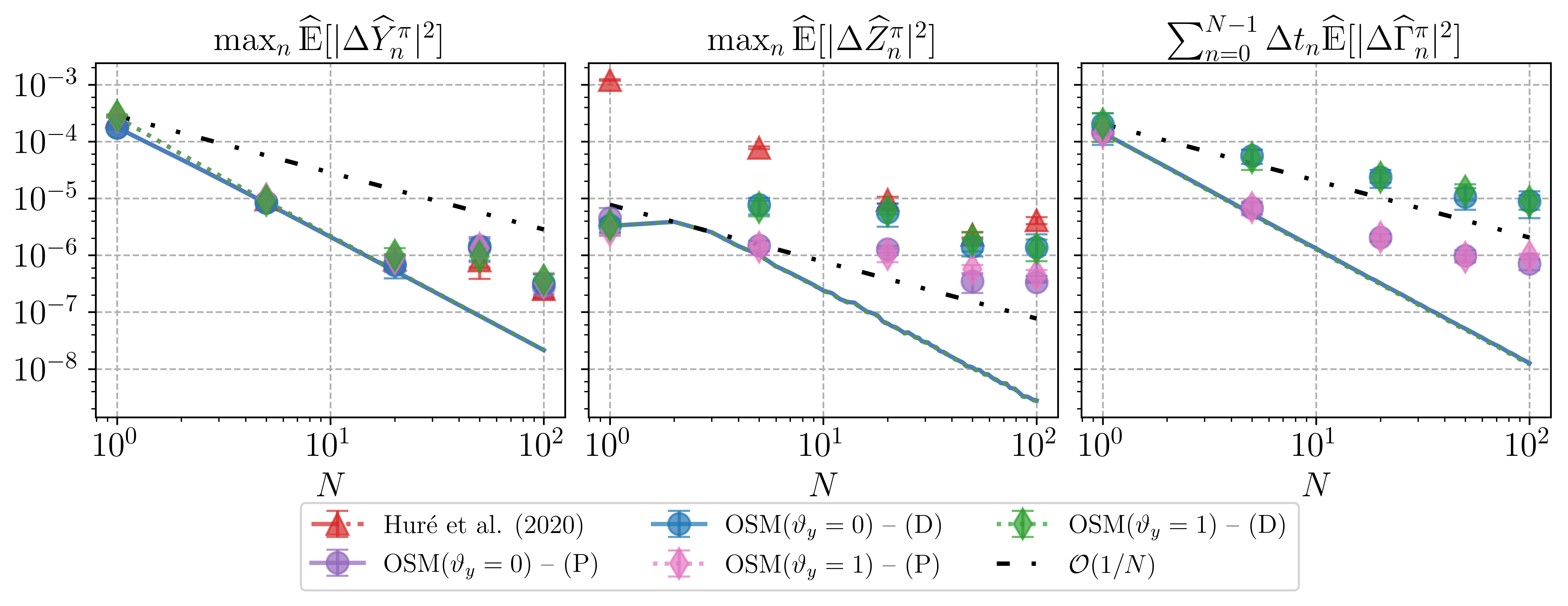
(a) BCOS and Deep BSDE, $d=1$. From left to right: maximum mean-squared approximation errors of $Y$ and $Z$; average mean-squared approximation error of $\Gamma$. Lines correspond to BCOS estimates, scattered error bars to the means and standard deviations of $5$ independent neural network regressions.

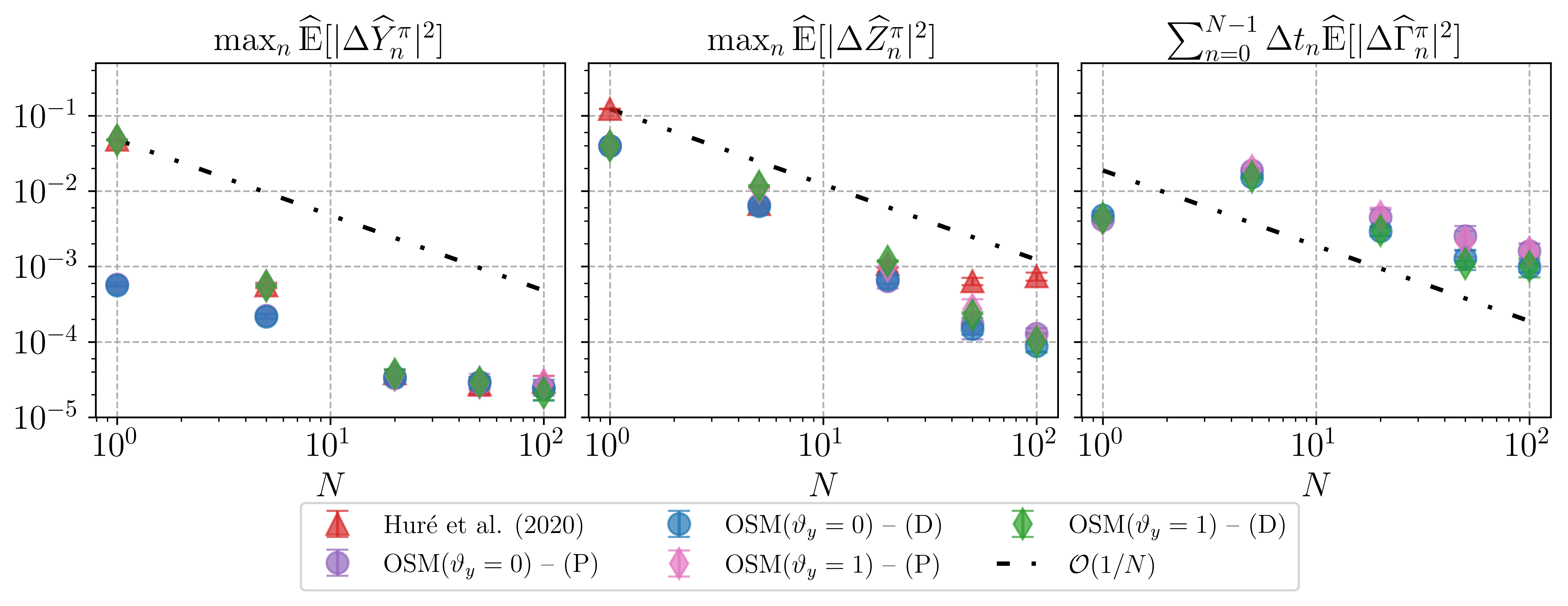
(b) Deep BSDE, $d=10$. From left to right: maximum mean-squared approximation errors of $Y$ and $Z$; average mean-squared approximation error of $\Gamma$. Means and standard deviations are calculated over $5$ independent runs of the algorithm.

Figure 1: Example 1 in Equation 6.2. Convergence of approximation errors. Mean-squared errors are calculated over an independent sample of $M=2^{10}$ realizations of the underlying Brownian motion.

Table 1: Example 1 in Equation 6.2, $d=10$, $N=100$. Summary of Deep BSDE estimates. Mean-squared errors are calculated over an independent sample of $M=2^{10}$ realizations of the underlying Brownian motion. Means and standard deviations (in parentheses) obtained over $5$ independent runs of the algorithm. Best estimates within one standard deviation highlighted in gray. $\Gamma$ estimates from Huré et al. in [27] are obtained via automatic differentiation.

	OSM($\vartheta_{y}=0$)		OSM($\vartheta_{y}=1$)		Huré et al. (2020)
	(P)	(D)	(P)	(D)
$|\Delta\widehat{Y}_{0}^{\pi}|/|Y_{0}|$	$$310-04$\left($310-04$\right)$	$$310-04$\left($210-04$\right)$	$$610-04$\left($210-04$\right)$	$$210-04$\left($210-04$\right)$	$$1.110-03$\left($410-04$\right)$
$|\Delta\widehat{Z}_{0}^{\pi}|/|Z_{0}|$	$$710-03$\left($310-03$\right)$	$$810-03$\left($210-03$\right)$	$$910-03$\left($210-03$\right)$	$$910-03$\left($510-03$\right)$	$$910-03$\left($210-03$\right)$
$|\Delta\widehat{\Gamma}_{0}^{\pi}|$	$$1.210-02$\left($310-03$\right)$	$$810-03$\left($310-03$\right)$	$$910-03$\left($110-03$\right)$	$$810-03$\left($210-03$\right)$	$$9.910+02$\left($810+01$\right)$
$\max_{n}\widehat{\mathds{E}}[|\Delta\widehat{Y}_{n}^{\pi}|^{2}]$	$$2.410-05$\left($510-06$\right)$	$$2.410-05$\left($710-06$\right)$	$$2.710-05$\left($810-06$\right)$	$$2.110-05$\left($410-06$\right)$	$$2.910-05$\left($610-06$\right)$
$\max_{n}\widehat{\mathds{E}}[|\Delta\widehat{Z}_{n}^{\pi}|^{2}]$	$$1.310-04$\left($210-05$\right)$	$$910-05$\left($110-05$\right)$	$$1.110-04$\left($210-05$\right)$	$$1.010-04$\left($310-05$\right)$	$$7.410-04$\left($910-05$\right)$
$\sum_{n=0}^{N-1}\Delta t_{n}\widehat{\mathds{E}}[|\Delta\widehat{\Gamma}_{n}^{\pi}|^{2}]$	$$810-04$\left($210-04$\right)$	$$5.010-04$\left($710-05$\right)$	$$810-04$\left($210-04$\right)$	$$510-04$\left($110-04$\right)$	$$5.010+03$\left($810+02$\right)$
runtime (s)	$$1.2010+03$\left($110+01$\right)$	$$1.4410+03$\left($210+01$\right)$	$$1.1910+03$\left($110+01$\right)$	$$1.4310+03$\left($510+01$\right)$	$$5.710+02$\left($310+01$\right)$

6.2 Example 2: Hamilton-Jacobi-Bellman with LQG control

The Hamilton-Jacobi-Bellman (HJB) equation is a non-linear PDE derived from Bellman’s dynamic programming principle, whose solution is the value function of a corresponding stochastic control problem. In what follows, we consider the linear-quadratic-Gaussian (LQG) control, which describes a linear system driven by additive noise [23]. The FBSDE system Equation 1.1, associated with the HJB equation has the following coefficients

$$\begin{split}\mu&=\mathbf{0}_{d},\qquad\sigma=\sqrt{2}I_{d},\qquad f(t,x,y,z)=\absolutevalue{z}^{2},\qquad g(x)=x^{T}Ax+v^{T}x+c,\end{split}$$ (6.4)

where $A\in\mathds{R}^{d\times d},v\in\mathds{R}^{d\times 1},c\in\mathds{R}$. Unlike in [23], the hereby considered terminal condition is a quadratic mapping of space. This choice is made so that we have access to semi-analytical, pathwise reference solutions $\{(Y_{t},Z_{t},\Gamma_{t})\}_{0\leq t\leq T}$. Indeed, considering the associated parabolic problem Equation 1.2, it is straightforward to show that the solution is given by

$$\begin{split}X_{t}=\sigma W_{t},\quad y(t,x)&=x^{T}P(t)x+Q^{T}(t)x+R(t),\\ z(t,x)&=\sigma\left(\left[P(t)+P^{T}(t)\right]x+Q(t)\right),\quad\gamma(t,x)=\sigma\left[P(t)+P^{T}(t)\right],\end{split}$$ (6.5)

where the purely time dependent functions $P:[0,T]\to\mathds{R}^{d\times d},Q:[0,T]\to\mathds{R}^{d\times 1},R:[0,T]\to\mathds{R}$ satisfy the following set of Riccati type ordinary differential equations (ODE)

$$\begin{split}\dot{P}(t)-\left[P(t)+P^{T}(t)\right]^{2}&=0,\quad\dot{Q}(t)-2\left[P(t)+P^{T}(t)\right]Q(t)=0,\quad\dot{R}(t)+\Tr{P(t)+P^{T}(t)}-\absolutevalue{Q(t)}^{2}=0,\\ P(T)&=A,\quad Q(T)=v,\quad R(T)=c,\end{split}$$ (6.6)

with $\dot{P}=\mathrm{d}P/\mathrm{d}t$, $\dot{Q}=\mathrm{d}Q/\mathrm{d}t$ and $\dot{R}=\mathrm{d}R/\mathrm{d}t$. The reference solution is then obtained by integrating Equation 6.6 over a refined time grid of $N_{\text{ODE}}=10^{4}$ intervals. We take $A=I_{d},v=\mathbf{0}_{d},c=0$, $T=0.5$ and fix $x_{0}=\mathbf{1}_{d}$. An interesting feature of the FBSDE system defined by Equation 6.4 is that the driver is independent of $Y$ meaning that the Malliavin BSDE in Equation 3.1d can be solved separately from the backward equation. Consequently, the discrete time approximations of $Z$ and $\Gamma$ in Equation 3.13 do not depend on $\vartheta_{y}$. Moreover, the driver is quadratically growing in $Z$, in particular, it is only Lipschitz continuous over compact domains. We pick $\vartheta_{y}=1/2$ and investigate the solution in $d\in\{1,50\}$.

In Figure 2 the regression errors of the Deep BSDE approach are assessed in $d=1$. The true regression targets in Equation 5.1 are benchmarked according to BCOS. In fact, at time step $n$, the corresponding cosine expansion coefficients are recovered by means of DCT, given neural network approximations $\widehat{Y}_{n+1}^{\pi},\widehat{Z}_{n+1}^{\pi},\widehat{\Gamma}_{n+1}^{\pi}$. These coefficients are subsequently plugged in Equation 5.7 to gather BCOS estimates. For large enough Fourier domains and sufficiently many Picard iterations, the COS error becomes negligible compared to the discretization component and the resulting estimates approximate the true regression labels $\widecheck{Y}_{n}^{\pi},\widecheck{Z}_{n}^{\pi},\widecheck{\Gamma}_{n}^{\pi}$. Hence, they can then be used to assess the regression errors induced by the Monte Carlo method. 2(a) depicts these regression errors over time for $N=100$. As it can be seen, the model of Huré et al. [27] and the OSM scheme result in similar regression error components for the $Y$ process. However, the regression errors of the $Z$ process are three orders of magnitude worse in case of the reference method [27], and in fact, dominate the total approximation error at $n=N-1$. In contrast, the OSM estimates – middle plot of 2(a) – exhibit the same order of regression error as for the $Y$ process. This demonstrates the advantageous conditional variance behavior of the corresponding OSM estimates, as pointed out in 3.1. The regression errors of the $\Gamma$ process show comparable figures. The cumulative regression errors, corresponding to the second term in Theorem 5.2, are collected in 3(b). In case of the model in [27], the cumulative regression error of the $Z$ process blows up as the mesh size $\absolutevalue{\pi}=T/N$ decreases. On the contrary, the cumulative regression errors in all processes $(Y,Z,\Gamma)$ are at a constant level of $\mathcal{O}(10^{-5})$ for the OSM scheme. In light of 5.1, this indicates that the chosen, finite network architecture incorporates a regression bias which cannot be further reduced. In our experiments, we found that it is difficult to decrease this component by changing the number of hidden layers $L$ or neurons per hidden layer $S_{l}$. Assessing this phenomenon requires a better understanding of both narrow UAT estimates and the convergence of SGD iterations.

In Figure 3 the $d=50$ dimensional case is depicted. In order to have dimension independent scales, relative mean-squared errors are reported. 3(a) collects the relative approximation error over the discretized time window when $N=100$. Compared to [27], the OSM estimates yield a significant improvement in each part of the solution triple. In particular, the approximation errors of the $Z$ process are three orders of magnitude better with both the parametrized (P) and automatic differentiated (D) approaches. In case of the $\Gamma$ process, two observations can be made. First, the corresponding curve demonstrates that naive automatic differentiation of the $Z$ approximations in [27] does not provide reliable $\Gamma$s. Moreover, it can be seen that the parametrized version (P) of the Deep BSDE approach given by Equation 5.15 provides an order of magnitude better average $\Gamma$ errors. The convergence of the total approximation errors is depicted in 3(b). The neural network regression estimates converge for both the parametrized (P) and the automatic differentiated (D) loss functions until $N=50$, when the regression bias becomes apparent. Additionally, the convergence of the $\Gamma$ approximations is significantly better in the parametrized case, suggesting that for such a quadratically scaling driver the last term of Equation 5.27 is a driving error component.

In Table 2 means and standard deviations of a collection of error measures are gathered, with respect to $5$ independent runs of the same regression Monte Carlo method, for both $d=1$ and $d=50$. The numbers are in line with the observations above. In particular, we highlight that the error terms corresponding to the $Z$ and $\Gamma$ approximations are four orders of magnitude better than in case of the reference method [27]. The parametrized version (P) of the Deep BSDE shows consistently better convergence. The total runtime of the neural network regression Monte Carlo approach is moderately increased between $d=1$ and $d=50$. In fact, the average execution time of a single SGD step for the parametrized (P) case in Equation 5.15 increases from $$2.810-3$($410-4$)$ to $$3.310-3$($410-4$)$ seconds in between $d=1$ and $d=50$. The same numbers for the automatic differentiated formulation (D) in Equation 5.16 are $$3.8$($410-4$)$ and $$4.410-3$($510-4$)$ seconds. These figures demonstrate the aforementioned methods’ scalability for high-dimensional FBSDE systems. Finally, we point out that the OSM estimates are robust over independent runs of the algorithm as showcased by the small standard deviations in Table 2.

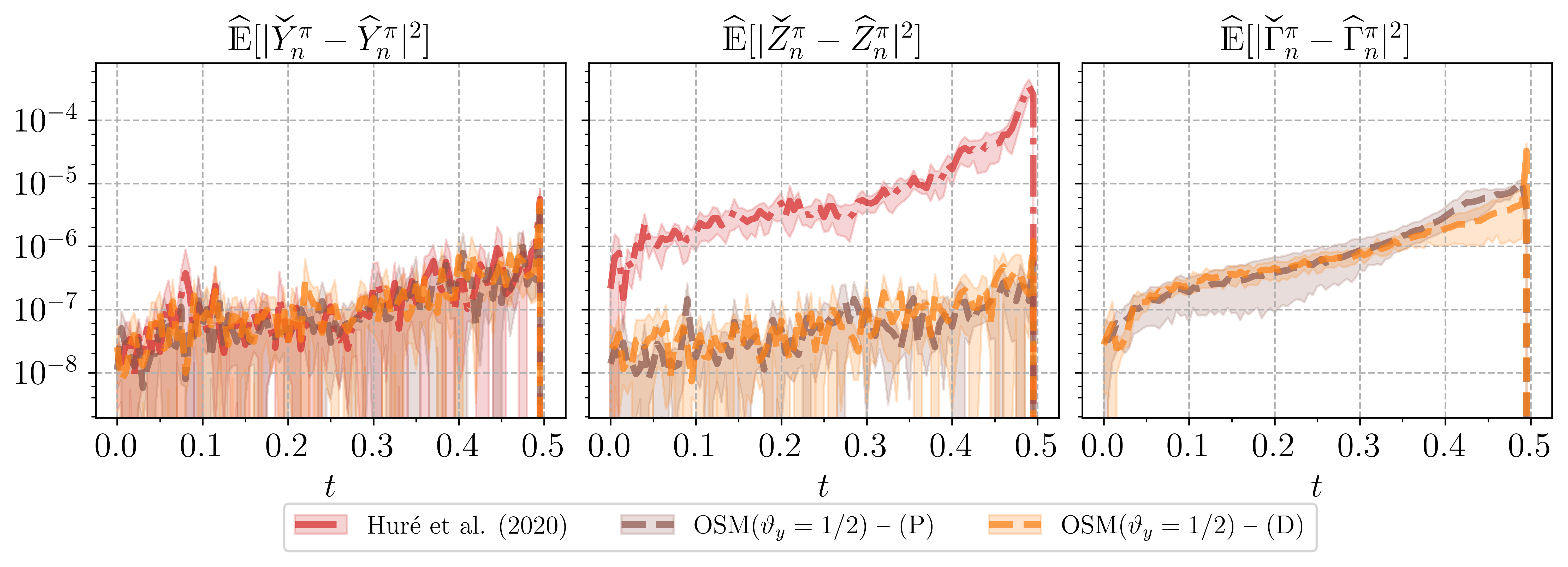
(a) Regression errors over time, $d=1$, $N=100$. From left to right: mean-squared regression errors of the $Y$, $Z$ and $\Gamma$ approximations over the discrete time window.

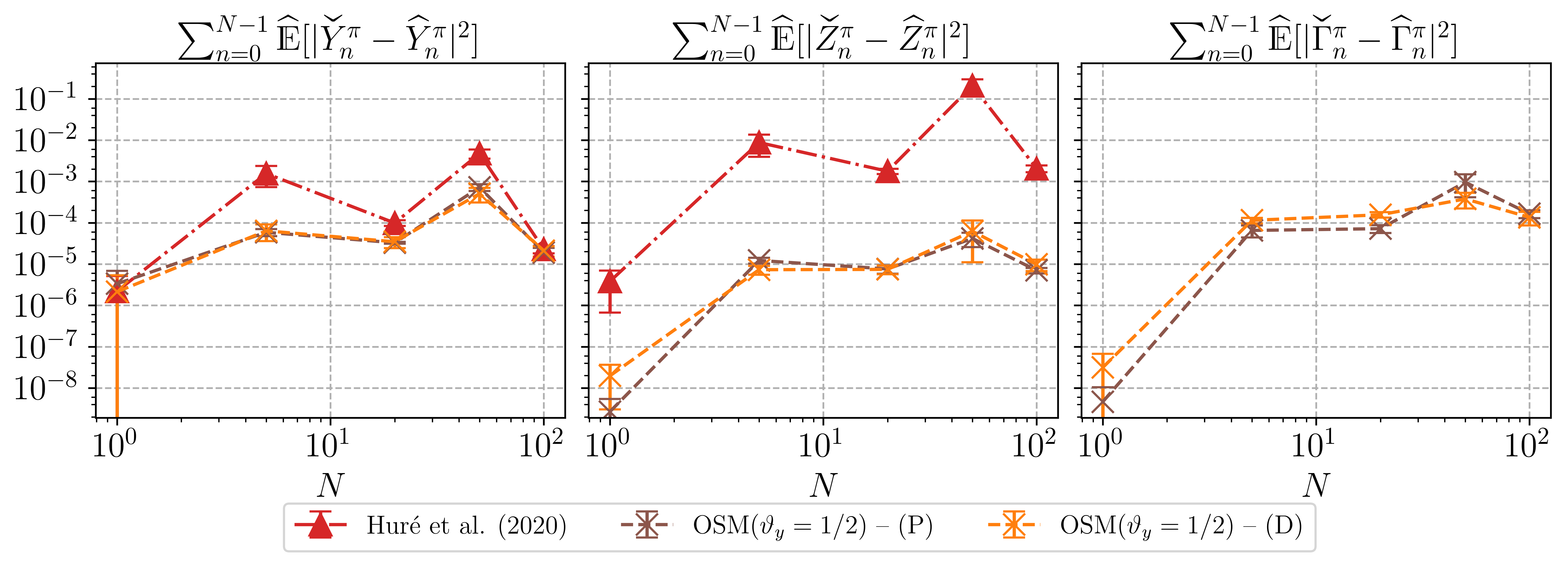
(b) Convergence of cumulative regression errors, $d=1$. From left to right: cumulative regression errors of the $Y$, $Z$ and $\Gamma$ approximations over the number of time steps $N$.

Figure 2: Example 2 in Equation 6.4. Neural network regression errors in $d=1$. The true regression targets of Equation 5.1 are identified by BCOS estimates. Mean-squared errors are calculated over an independent sample of $M=2^{10}$ realizations of the underlying Brownian motion. Means and standard deviations are obtained over $5$ independent runs of the algorithm.

(a) Relative approximation errors over time, $d=50$, $N=100$. From left to right: relative mean-squared approximation errors of $Y,Z$ and $\Gamma$ over the discrete time window.

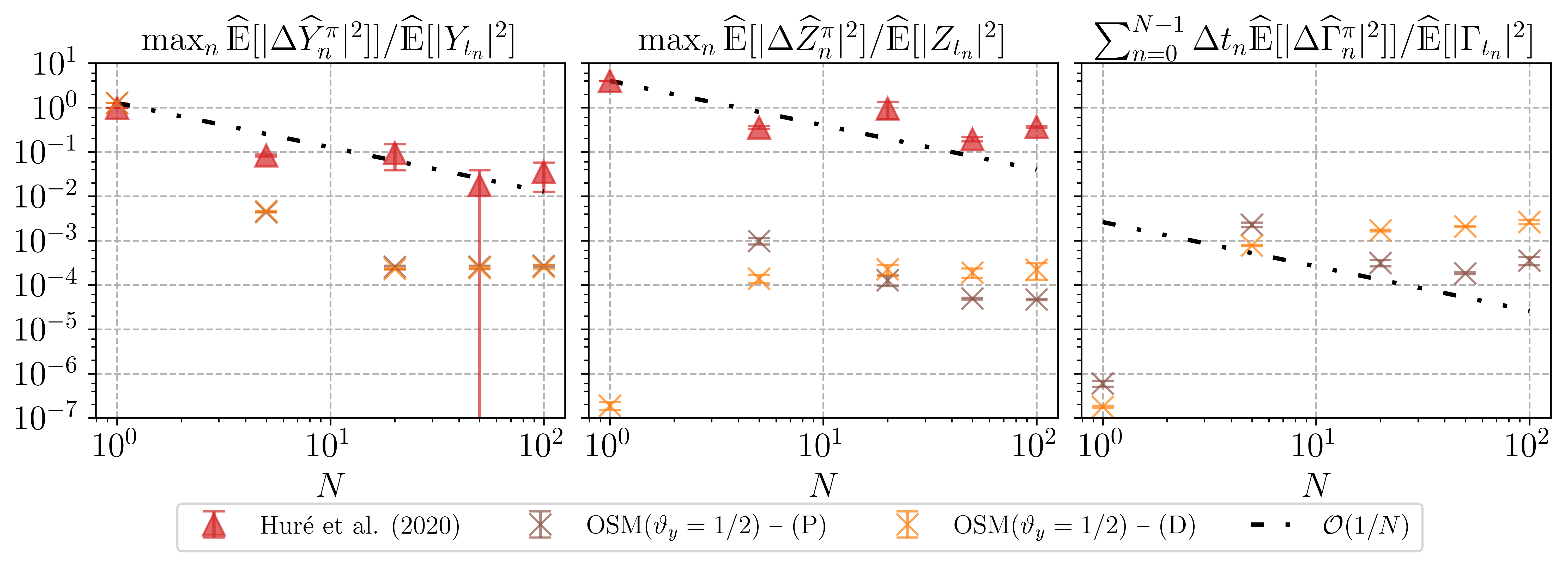
(b) Convergence of relative approximation errors, $d=50$. From left to right: maximum relative mean-squared error of the $Y$, $Z$ approximations; average relative mean-squared error of the $\Gamma$ approximations.

Figure 3: Example 2 in Equation 6.4. $d=50$. Relative approximation errors. Mean-squared errors are calculated over an independent sample of $M=2^{10}$ realizations of the underlying Brownian motion. Means and standard deviations are obtained over $5$ independent runs of the algorithm. $\Gamma$ estimates from Huré et al. in [27] are obtained via automatic differentiation.

Table 2: Example 2 in Equation 6.4. Summary of Deep BSDE estimates. Mean-squared errors are calculated over an independent sample of $M=2^{10}$ realizations of the underlying Brownian motion. Means and standard deviations (in parentheses) obtained over $5$ independent runs of the algorithm. Best estimates within one standard deviation highlighted in gray. $\Gamma$ estimates from Huré et al. in [27] are obtained via automatic differentiation.

(a) $d=1,N=100$.

	OSM($\vartheta_{y}=1/2$)		Huré et al. (2020)
	(P)	(D)
$|\Delta\widehat{Y}_{0}^{\pi}|/|Y_{0}|$	$$1.110-03$\left($510-04$\right)$	$$210-03$\left($110-03$\right)$	$$1.510-03$\left($310-04$\right)$
$|\Delta\widehat{Z}_{0}^{\pi}|/|Z_{0}|$	$$1.310-04$\left($910-05$\right)$	$$810-05$\left($910-05$\right)$	$$110-03$\left($110-03$\right)$
$|\Delta\widehat{\Gamma}_{0}^{\pi}|/|\Gamma_{0}|$	$$1.010-04$\left($510-05$\right)$	$$210-04$\left($110-04$\right)$	$$1.0510+00$\left($710-02$\right)$
$\max_{n}\widehat{\mathds{E}}[|\Delta\widehat{Y}_{n}^{\pi}|^{2}]$	$$810-06$\left($210-06$\right)$	$$810-06$\left($310-06$\right)$	$$1.110-04$\left($110-05$\right)$
$\max_{n}\widehat{\mathds{E}}[|\Delta\widehat{Z}_{n}^{\pi}|^{2}]$	$$810-07$\left($310-07$\right)$	$$1.410-06$\left($610-07$\right)$	$$6.410-03$\left($310-04$\right)$
$\sum_{n=0}^{N-1}\Delta t_{n}\widehat{\mathds{E}}[|\Delta\widehat{\Gamma}_{n}^{\pi}|^{2}]$	$$810-07$\left($410-07$\right)$	$$2.810-06$\left($910-07$\right)$	$$5.510-03$\left($710-04$\right)$
runtime (s)	$$1.1810+03$\left($410+01$\right)$	$$1.4110+03$\left($310+01$\right)$	$$5.710+02$\left($410+01$\right)$

(b) $d=50,N=100$.

	OSM($\vartheta_{y}=1/2$)		Huré et al. (2020)
	(P)	(D)
$|\Delta\widehat{Y}_{0}^{\pi}|/|Y_{0}|$	$$810-04$\left($510-04$\right)$	$$110-03$\left($110-03$\right)$	$$1.710-01$\left($810-02$\right)$
$|\Delta\widehat{Z}_{0}^{\pi}|/|Z_{0}|$	$$5.010-03$\left($510-04$\right)$	$$1.410-02$\left($310-03$\right)$	$$2.810-01$\left($710-02$\right)$
$|\Delta\widehat{\Gamma}_{0}^{\pi}|/|\Gamma_{0}|$	$$3.110-02$\left($210-03$\right)$	$$4.910-02$\left($710-03$\right)$	$$3.510+00$\left($110-01$\right)$
$\max_{n}\widehat{\mathds{E}}[|\Delta\widehat{Y}_{n}^{\pi}|^{2}]$	$$2.710+00$\left($110-01$\right)$	$$2.510+00$\left($310-01$\right)$	$$710+01$\left($410+01$\right)$
$\max_{n}\widehat{\mathds{E}}[|\Delta\widehat{Z}_{n}^{\pi}|^{2}]$	$$3.410-02$\left($110-03$\right)$	$$3.110-02$\left($310-03$\right)$	$$2.810+02$\left($110+01$\right)$
$\sum_{n=0}^{N-1}\Delta t_{n}\widehat{\mathds{E}}[|\Delta\widehat{\Gamma}_{n}^{\pi}|^{2}]$	$$4.110-04$\left($610-05$\right)$	$$3.310-03$\left($210-04$\right)$	$$2.910+00$\left($210-01$\right)$
runtime (s)	$$1.3610+03$\left($110+01$\right)$	$$1.6210+03$\left($410+01$\right)$	$$6.1610+02$\left($110+01$\right)$

6.3 Example 3: space-dependent diffusion coefficients

Our final example is taken from [36, 41] and it is meant to demonstrate that the conditions in 4.1 can be substantially relaxed. The FBSDE system Equation 1.1 is defined by the following coefficients

$$\begin{split}\mu_{i}(t,x)&=\frac{(1+x_{i}^{2})}{\left(2+x_{i}^{2}\right)^{3}},\quad\sigma_{ij}(t,x)=\frac{1+x_{i}x_{j}}{2+x_{i}x_{j}}\delta_{ij},\\ f(t,x,y,z)&=\begin{aligned} &\frac{1}{\lambda(t+\tau)}\exp(-\frac{x^{T}x}{\lambda(t+\tau)})\left[4\sum_{i=1}^{d}\frac{x_{i}^{2}(1+x_{i}^{2})}{(2+x_{i}^{2})^{3}}+\sum_{i=1}^{d}\frac{(1+x_{i}^{2})^{2}}{(2+x_{i}^{2})^{2}}\left(1-2\frac{x_{i}^{2}}{\lambda(t+\tau)}\right)-\sum_{i=1}^{d}\frac{x_{i}^{2}}{t+\tau}\right]\\ &+\sqrt{\frac{1+y^{2}+\exp(-\frac{2x^{T}x}{\lambda(t+\tau)})}{1+2y^{2}}}\sum_{i=1}^{d}\frac{z_{i}x_{i}}{(2+x_{i}^{2})^{2}},\qquad g(x)=\exp(-\frac{x^{T}x}{\lambda(T+\tau)}).\end{aligned}\end{split}$$ (6.7)

The analytical solutions are given by

$$\begin{split}y(t,x)&=\exp(-\frac{x^{T}x}{\lambda(t+\tau)}),\quad z_{j}(t,x)=-\frac{1+x_{j}^{2}}{2+x_{j}^{2}}\frac{2\exp(-\frac{x^{T}x}{\lambda(t+\tau)})}{\lambda(t+\tau)}x_{j},\quad\gamma_{ij}(t,x)=\partial_{j}z_{i}(t,x).\end{split}$$ (6.8)

We use $T=10,\lambda=10,\tau=1$, $d=1$ and fix $x_{0}=\mathbf{1}_{d}$. Notice that $\mu$ and $\sigma$ are both $C^{2}_{b}$. In conjecture with Appendix A, this implies that the Euler-Maruyama schemes in Equation 3.2 and Equation 3.5 have an $\mathds{L}^{2}$ convergence rate of order $1/2$. Additionally, by Itô’s formula, the unique solution of the SDE is given by the closed form expression [36]

$$X_{t}=\Lambda(x_{0}+\arctan(x_{0})+W_{t}),$$ (6.9)

where $\Lambda:\mathds{R}\to\mathds{R}$ is defined implicitly $\Lambda(r)+\arctan(r)\coloneqq r$ for any $r\in\mathds{R}$, and applied element-wise. It is straightforward to check that $\Lambda\in C_{b}^{1}(\mathds{R};\mathds{R})$, in particular $\Lambda^{{}^{\prime}}(r)=\frac{1+\Lambda^{2}(r)}{2+\Lambda^{2}(r)}$ implying that $\Lambda$ is a bijective. In light of the Malliavin chain rule formula in 2.1, we then also have

$$D_{s}X_{t}=\frac{1+\Lambda^{2}(x+\arctan(x)+W_{t})}{2+\Lambda^{2}(x+\arctan(x)+W_{t})}\mathds{1}_{s\leq t}.$$ (6.10)

We assess the convergence of the Euler-Maruyama estimates in Equation 3.2–Equation 3.5 by solving the non-linear equation in Equation 6.9 for each realization of the Brownian motion. The results of the numerical simulations in $d=1$ are given in Figure 4 for the parametrized Deep BSDE case and $\vartheta_{y}=0,1/2,1$. We see that, in line with Appendix A, $D_{n}X_{n+1}^{\pi}$ inherits the convergence rate of $X_{n}^{\pi}$. The convergence rates of $(\widehat{Y}_{n}^{\pi},\widehat{Z}_{n}^{\pi},\widehat{\Gamma}_{n}^{\pi})$ are of the same order as in Theorem 5.2. The BCOS estimates and the Deep BSDE approach exhibit coinciding error figures until a magnitude of $\mathcal{O}(10^{-6})$ is reached, when the regression bias becomes apparent. Similar convergence behavior is observed in high-dimensions. The results suggest that the convergence of the OSM scheme can be extended to the non-additive noise case.

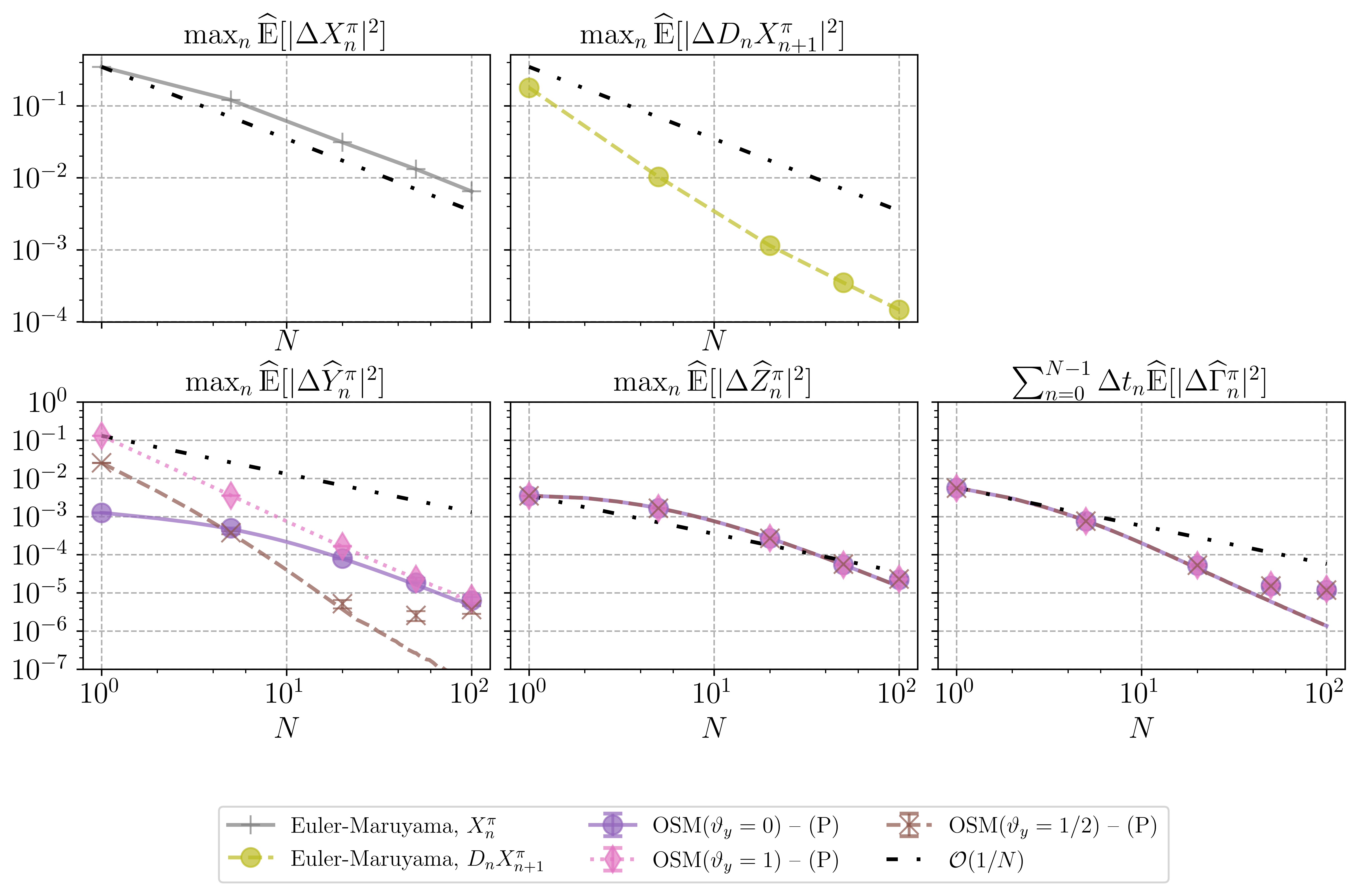
Figure 4: Example 3 in Equation 6.7. Convergence of approximation errors for $d=1$. From left to right, top to bottom: maximum mean-squared errors of Euler-Maruyama approximations of $X$ and $DX$; maximum mean-squared approximation errors of $Y$ and $Z$; average mean-squared approximation error of $\Gamma$. Lines correspond to BCOS estimates, scattered error bars to the means and standard deviations of $5$ independent neural network regressions. The mean errors are obtained over an independent sample of $M=2^{10}$ trajectories of the underlying Brownian motion.

7 Conclusion

In this paper we introduced the One Step Malliavin (OSM) scheme, a new discretization for Malliavin differentiable FBSDE systems where the control process is estimated by solving the linear BSDE driving the Malliavin derivatives of the solution pair. The main contributions can be summarized as follows. The discretization in Equation 3.13 includes $\Gamma$ estimates, linked to the Hessian matrix of the associated parabolic problem. In Theorem 4.1 we have shown that under standard Lipschitz assumptions and additive noise in the forward diffusion, the aforementioned discrete time approximations admit to an $\mathds{L}^{2}$ convergence of order $1/2$. We gave two fully-implementable schemes. In case of one-dimensional problems, we extended the BCOS method [40], and gathered approximations via Fourier cosine expansions in Equation 5.7. For high-dimensional equations, similarly to recent Deep BSDE methods [23, 27], we formulated a neural network regression Monte Carlo approach, where the corresponding processes of the solution triple are parametrized by fully-connected, feedforward neural networks. We carried out a complete regression error analysis in Theorem 5.2 and showed that the neural network parametrizations are consistent with the discretization, in terms of regression biases controlled by the universal approximation property. We supported our theoretical findings by numerical experiments and demonstrated the accuracy and robustness of the proposed approaches for a range of high-dimensional problems. Using BCOS estimates as benchmarks for one-dimensional equations, we empirically assessed the regression errors induced by stochastic gradient descent. Our findings with the Deep BSDE approach showcase accurate approximations for each process in Equation 5.1, and in particular exhibit significantly improved approximations of the $Z$ process for heavily control dependent equations.

Acknowledgments

The first author would like to thank Adam Andersson for the fruitful discussions in the early stages of this work. The first author also acknowledges financial support from the Peter Paul Peterich Foundation via the TU Delft University Fund.

Appendix A Convergence of $D_{n}X_{n+1}^{\pi}$

We show the convergence of $D_{n}X_{n+1}^{\pi}$ estimates of the Euler-Maruyama discretization Equation 3.5 under the assumptions

1. $\sigma$ is uniformly bounded;

2. $\mu\in C_{b}^{0,1}(\mathds{R}^{d\times 1};\mathds{R})$, $\sigma\in C_{b}^{0,1}(\mathds{R}^{d\times 1};\mathds{R}^{d\times d})$. In particular both of them are Lipschitz continuous in $x.$

From the estimation Equation 3.5 and the linear SDE of the Malliavin derivative in Equation 3.1c – using the inequality $(a+b+c)^{2}\leq 4(a^{2}+b^{2}+c^{2})$, on top of the $L^{2}([0,T];\mathds{R}^{d\times d})$ Cauchy-Schwarz inequality and Itô’s isometry –, it follows

$$\mathbb{E}\left[\absolutevalue{D_{t_{n}}X_{t_{n+1}}-D_{n}X_{n+1}^{\pi}}^{2}\right]\leq\begin{aligned} &4\mathbb{E}\left[\absolutevalue{\sigma(t_{n},X_{t_{n}})-\sigma(t_{n},X_{n}^{\pi})}^{2}\right]\\ &+4\Delta t_{n}\mathbb{E}\left[\int_{t_{n}}^{t_{n+1}}\absolutevalue{\nabla_{x}\mu(r,X_{r})D_{t_{n}}X_{r}-\nabla_{x}\mu(t_{n},X_{n}^{\pi})\sigma(t_{n},X_{n}^{\pi})}^{2}\mathrm{d}r\right]\\ &+4\mathbb{E}\left[\int_{t_{n}}^{t_{n+1}}\absolutevalue{\nabla_{x}\sigma(r,X_{r})D_{t_{n}}X_{r}-\nabla_{x}\sigma(t_{n},X_{n}^{\pi})\sigma(t_{n},X_{n}^{\pi})}^{2}\mathrm{d}r\right].\end{aligned}$$ (A.1)

Bounded continuous differentiability in ($\widetilde{\mathbf{A}}^{\sigma,\mu}_{2}$), in particular, implies Lipschitz continuity. Furthermore, by the uniform boundedness of the diffusion coefficient and the mean-squared continuity of $D_{t_{n}}X$ in Equation 2.6, we gather

$$\mathbb{E}\left[\absolutevalue{D_{t_{n}}X_{t_{n+1}}-D_{n}X_{n+1}^{\pi}}^{2}\right]\leq 4L_{\sigma}^{2}\mathbb{E}\left[\absolutevalue{X_{t_{n}}-X_{n}^{\pi}}^{2}\right]+C\Delta t_{n},$$ (A.2)

for any $\Delta t_{n}<1$. Then, due to the discretization error of the Euler-Maruyama estimates given by Equation 3.2, we conclude $\limsup_{\absolutevalue{\pi}\to 0}\frac{1}{\absolutevalue{\pi}}\mathbb{E}\left[\absolutevalue{D_{t_{n}}X_{t_{n+1}}-D_{n}X_{n+1}^{\pi}}^{2}\right]<\infty$.

Appendix B Integration by parts formulas

For the formula in Equation 5.5 we refer to [40, A.1]. In order to prove Equation 5.6, let $v:[0,T]\times\mathds{R}\to\mathds{R}$ and consider

$$\mathbb{E}_{n}^{x}\left[v(t_{n+1},X_{n+1}^{\pi}(\Delta W_{n}))\Delta W_{n}^{2}\right]=\mathbb{E}_{n}^{x}\left[\frac{1}{\sqrt{2\pi\Delta t_{n}}}\int_{\mathds{R}}v(t_{n+1},X_{n+1}^{\pi}(\nu)\nu^{2}e^{-\frac{1}{2\Delta t_{n}}\nu^{2}}\mathrm{d}\nu\right],$$ (B.1)

with the Euler-Maruyama approximations $X_{n+1}^{\pi}(\Delta W_{n})=x+\mu(t_{n},x)\Delta t_{n}+\sigma(t_{n},x)\Delta W_{n}$. For a sufficiently smooth $v$, integration by parts implies

$$\mathbb{E}_{n}^{x}\left[\frac{1}{\sqrt{2\pi\Delta t_{n}}}\int_{\mathds{R}}v(t_{n+1},X_{n+1}^{\pi})\nu^{2}e^{-\frac{1}{2\Delta t_{n}}\nu^{2}}\mathrm{d}\nu\right]=\begin{aligned} \mathds{E}_{n}^{x}\Bigg{[}\frac{1}{\sqrt{2\pi\Delta t_{n}}}\Big{\{}&-\Delta t_{n}\left[\nu v(t_{n+1},X_{n+1}^{\pi})e^{-\nu^{2}/(2\Delta t_{n})}\right]_{-\infty}^{+\infty}\\ &+\Delta t_{n}\int_{\mathds{R}}v(t_{n+1},X_{n+1}^{\pi})e^{-\frac{1}{2\Delta t_{n}}\nu^{2}}\mathrm{d}\nu\\ &+\Delta t_{n}\sigma(t_{n},x)\int_{\mathds{R}}\partial_{x}v(t_{n+1},X_{n+1}^{\pi})\nu e^{-\frac{1}{2\Delta t_{n}}\nu^{2}}\mathrm{d}\nu\Big{\}}\Bigg{]},\end{aligned}$$ (B.2)

For a $v$ with sufficient radial decay, we therefore conclude that

$$\mathbb{E}_{n}^{x}\left[v(t_{n+1},X_{n+1}^{\pi})\Delta W_{n}^{2}\right]=\Delta t_{n}\mathbb{E}_{n}^{x}\left[v(t_{n+1},X_{n+1}^{\pi})\right]+\Delta t_{n}^{2}\sigma^{2}(t_{n},x)\mathbb{E}_{n}^{x}\left[\partial_{xx}^{2}v(t_{n+1},X_{n+1}^{\pi})\right],$$ (B.3)

by the estimate in Equation 5.5.

Thereupon, given a cosine expansion approximation of $v(t_{n+1},\rho)\approx\sideset{}{{}^{\prime}}{\sum}_{k=0}^{K-1}\mathcal{V}_{k}(t_{n+1})\cos(k\pi\frac{\rho-a}{b-a})$, the corresponding spatial derivative approximations are given by $\partial_{x}v(t_{n+1},\rho)\approx\sideset{}{{}^{\prime}}{\sum}_{k=0}^{K-1}-\mathcal{V}_{k}(t_{n+1})\frac{k\pi}{b-a}\sin(k\pi\frac{\rho-a}{b-a}),\quad\partial_{xx}^{2}v(t_{n+1},\rho)\approx\sideset{}{{}^{\prime}}{\sum}_{k=0}^{K-1}-\mathcal{V}_{k}(t_{n+1})\left(\frac{k\pi}{b-a}\right)^{2}\cos(k\pi\frac{\rho-a}{b-a}).$ Then the approximations in Equation 5.5–Equation 5.6 follow from the expressions $\mathbb{E}_{n}^{x}\left[\sin(k\pi\frac{X_{n+1}^{\pi}-a}{b-a})\right]=\Im{\Phi\left(k|x\right)},\quad\mathbb{E}_{n}^{x}\left[\cos(k\pi\frac{X_{n+1}^{\pi}-a}{b-a})\right]=\Re{\Phi\left(k|x\right)},$ where $\Phi(k|x)$ is defined as in subsection 5.1.

Multi-dimensional extensions.

In case the underlying forward process is a $\mathds{R}^{d\times 1}$-dimensional Brownian motion, the following extension can be given. Let $v:[0,T]\times\mathds{R}^{d\times 1}\to\mathds{R}$ be a scalar-valued function. Then reasoning similar to [40, A.1] shows that $\mathbb{E}_{n}\left[\left(\Delta W_{n}\right)_{i1}v(t_{n+1},X_{n+1})\right]=\sum_{k=1}^{d}\Delta t_{n}\mathbb{E}_{n}\left[\partial_{k}v(t_{n+1},X_{n+1}^{\pi})\right]\left(\sigma(t_{n+1},X_{n+1}^{\pi})\right)_{ki}$. In matrix notation

$$\left(\mathbb{E}_{n}\left[\Delta W_{n}v(t_{n+1},X_{n+1}^{\pi})\right]\right)^{T}=\Delta t_{n}\mathbb{E}_{n}\left[\nabla_{x}v(t_{n+1},X_{n+1}^{\pi})\right]\sigma(t_{n+1},X_{n+1}).$$ (B.4)

Alternatively, for a vector-valued mapping $\psi:[0,T]\times\mathds{R}^{d\times 1}\to\mathds{R}^{1\times d}$, similar arguments give the following, component-wise formula $\mathbb{E}_{n}\left[\left(\Delta W_{n}\right)_{i1}\left(\psi(t_{n+1},X_{n+1})\right)_{1j}\right]=\sum_{k=1}^{d}\Delta t_{n}\mathbb{E}_{n}\left[\partial_{k}\left(\psi(t_{n+1},X_{n+1}^{\pi})\right)_{1j}\right]\left(\sigma(t_{n},X_{n}^{\pi})\right)_{ki}$. In matrix notation

$$\left(\mathbb{E}_{n}\left[\Delta W_{n}\psi(t_{n+1},X_{n+1}^{\pi})\right]\right)^{T}=\Delta t_{n}\mathbb{E}_{n}\left[\nabla_{x}\psi(t_{n+1},X_{n+1}^{\pi})\right]\sigma(t_{n},X_{n}^{\pi}),$$ (B.5)

where $\nabla_{x}\psi$ is the Jacobian matrix of $\psi$.

Appendix C BCOS estimates

Let us fix $d=1$. The BCOS approximations of the OSM scheme in Equation 5.7 can be derived as follows. Using the definition in Equation 5.8 and the Euler-Maruyama estimates in Equation 3.5, the $\Gamma$ estimates in Equation 5.1b can be written according to

$$D_{n}\widecheck{Z}_{n}^{\pi}=\widecheck{\gamma}_{n}^{\pi}(x)\sigma(t_{n},x) =\begin{aligned} &\frac{1}{\Delta t_{n}}\sigma(t_{n},x)\left(1+\Delta t_{n}\partial_{x}\mu(t_{n},x)\right)\mathbb{E}_{n}^{x}\left[\Delta W_{n}w_{n+1}^{\pi}({\widehat{\mathbf{X}}}_{n+1}^{\pi})\right]\\ &+\frac{1}{\Delta t_{n}}\sigma(t_{n},x)\partial_{x}\sigma(t_{n},x)\mathbb{E}_{n}^{x}\left[\Delta W_{n}^{2}w_{n+1}^{\pi}({\widehat{\mathbf{X}}}_{n+1}^{\pi})\right]\\ &+\mathbb{E}_{n}^{x}\left[\Delta W_{n}\partial_{z}f(t_{n+1},{\widehat{\mathbf{X}}}_{n+1}^{\pi})\right]\widecheck{\gamma}^{\pi}_{n}(x)\sigma(t_{n},x).\end{aligned}$$ (C.1)

A cosine expansion approximation for $w_{n+1}^{\pi}({\widehat{\mathbf{X}}}_{n+1}^{\pi})$ and $\partial_{z}f(t_{n+1},{\widehat{\mathbf{X}}}_{n+1}^{\pi})$ can be obtained by means of DCT, yielding approximations $\{\widehat{\mathcal{W}}_{k}(t_{n+1})\}_{k=0,\dots,K-1}$, $\{\widehat{\mathcal{F}}_{k}^{z}(t_{n+1})\}_{k=0,\dots,K-1}$ respectively. Consequently, plugging these approximations combined with the integration by parts formulas in Equation 5.5–Equation 5.6, in the estimate above yields

$$\widehat{\gamma}_{n}^{\pi}(x)\sigma(t_{n},x)=\begin{aligned} &-\sigma^{2}(t_{n},x)(1+\partial_{x}\mu(t_{n},x)\Delta t_{n})\sideset{}{{}^{\prime}}{\sum}_{k=0}^{K-1}\frac{k\pi}{b-a}\widehat{\mathcal{W}}_{k}(t_{n+1})\Im{\Phi(k|x)}\\ &+\sigma(t_{n},x)\partial_{x}\sigma(t_{n},x)\sideset{}{{}^{\prime}}{\sum}_{k=0}^{K-1}\widehat{\mathcal{W}}_{k}(t_{n+1})\Re{\Phi(k|x)}\\ &-\Delta t_{n}\sigma^{3}(t_{n},x)\partial_{x}\sigma(t_{n},x)\sideset{}{{}^{\prime}}{\sum}_{k=0}^{K-1}\left(\frac{k\pi}{b-a}\right)^{2}\widehat{\mathcal{W}}_{k}(t_{n+1})\Re{\Phi(k|x)}\\ &-\widehat{\gamma}_{n}^{\pi}(x)\Delta t_{n}\sigma^{2}(t_{n},x)\sideset{}{{}^{\prime}}{\sum}_{k=0}^{K-1}\frac{k\pi}{b-a}\widehat{\mathcal{F}}^{z}_{k}(t_{n+1})\Im{\Phi(k|x)}.\end{aligned}$$ (C.2)

The approximation $D_{n}\widehat{Z}_{n}^{\pi}=\widehat{\Gamma}_{n}^{\pi}\sigma(t_{n},X_{n}^{\pi})$ subsequently follows. The coefficients $\{\widehat{\mathcal{DZ}}_{k}(t_{n+1})\}_{k=0,\dots,K-1}$ are calculated by DCT and subsequently plugged into the approximations of the $Z$ process, which follows analogously using the formulas in Equation 5.4–Equation 5.5. The approximation of the $Y$ process in Equation 5.1d is identical to [40] and therefore omitted.

References

• [1] Samu Alanko and Marco Avellaneda “Reducing variance in the numerical solution of BSDEs” In Comptes Rendus Mathematique 351.3, 2013, pp. 135–138 DOI: 10.1016/j.crma.2013.02.010
• [2] Jimmy Lei Ba, Jamie Ryan Kiros and Geoffrey E. Hinton “Layer Normalization” arXiv: 1607.06450 In arXiv:1607.06450 [cs, stat], 2016 URL: http://arxiv.org/abs/1607.06450
• [3] Vlad Bally and Gilles Pagès “A quantization algorithm for solving multidimensional discrete-time optimal stopping problems” Publisher: Bernoulli Society for Mathematical Statistics and Probability In Bernoulli 9.6, 2003, pp. 1003–1049 DOI: 10.3150/bj/1072215199
• [4] Christian Beck, E. Weinan and Arnulf Jentzen “Machine Learning Approximation Algorithms for High-Dimensional Fully Nonlinear Partial Differential Equations and Second-order Backward Stochastic Differential Equations” In Journal of Nonlinear Science, 2019 DOI: 10.1007/s00332-018-9525-3
• [5] Christian Bender and Robert Denk “A forward scheme for backward SDEs” In Stochastic Processes and their Applications 117.12, 2007, pp. 1793–1812 DOI: 10.1016/j.spa.2007.03.005
• [6] Christian Bender and Jessica Steiner “Least-Squares Monte Carlo for Backward SDEs” In Numerical Methods in Finance Berlin, Heidelberg: Springer Berlin Heidelberg, 2012, pp. 257–289 DOI: 10.1007/978-3-642-25746-9_8
• [7] Bruno Bouchard and Nizar Touzi “Discrete-time approximation and Monte-Carlo simulation of backward stochastic differential equations” In Stochastic Processes and their Applications 111.2, 2004, pp. 175–206 DOI: 10.1016/j.spa.2004.01.001
• [8] Philippe Briand and Céline Labart “Simulation of BSDEs by Wiener chaos expansion” Publisher: The Institute of Mathematical Statistics In The Annals of Applied Probability 24.3, 2014, pp. 1129–1171 DOI: 10.1214/13-AAP943
• [9] Jean-François Chassagneux and Adrien Richou “Numerical simulation of quadratic BSDEs” Publisher: Institute of Mathematical Statistics In The Annals of Applied Probability 26.1, 2016, pp. 262–304 URL: http://www.jstor.org/stable/43859598
• [10] Yangang Chen and Justin W.. Wan “Deep neural network framework based on backward stochastic differential equations for pricing and hedging American options in high dimensions” In Quantitative Finance 21.1, 2021, pp. 45–67 DOI: 10.1080/14697688.2020.1788219
• [11] Patrick Cheridito, H. Soner, Nizar Touzi and Nicolas Victoir “Second-order backward stochastic differential equations and fully nonlinear parabolic PDEs” In Communications on Pure and Applied Mathematics, 2007 DOI: 10.1002/cpa.20168
• [12] George Cybenko “Approximation by superpositions of a sigmoidal function” Publisher: Springer In Mathematics of control, signals and systems 2.4, 1989, pp. 303–314 DOI: 10.1007/BF02551274
• [13] François Delarue and Stéphane Menozzi “A forward - Backward stochastic algorithm for quasi-linear PDES” In The Annals of Applied Probability, 2006 DOI: 10.1214/105051605000000674
• [14] Nicole El Karoui, Shige Peng and Marie Claire Quenez “Backward stochastic differential equations in finance” Publisher: Wiley Online Library In Mathematical finance 7.1, 1997, pp. 1–71
• [15] Arash Fahim, Nizar Touzi and Xavier Warin “A probabilistic numerical method for fully nonlinear parabolic PDEs” Publisher: Institute of Mathematical Statistics In The Annals of Applied Probability 21.4, 2011, pp. 1322–1364 DOI: 10.1214/10-AAP723
• [16] F. Fang and C.. Oosterlee “A Novel Pricing Method for European Options Based on Fourier-Cosine Series Expansions” Publisher: Society for Industrial and Applied Mathematics In SIAM Journal on Scientific Computing 31.2, 2009, pp. 826–848 DOI: 10.1137/080718061
• [17] Masaaki Fujii, Akihiko Takahashi and Masayuki Takahashi “Asymptotic Expansion as Prior Knowledge in Deep Learning Method for High dimensional BSDEs” In Asia-Pacific Financial Markets 26.3, 2019, pp. 391–408 DOI: 10.1007/s10690-019-09271-7
• [18] Maximilien Germain, Huyen Pham and Xavier Warin “Approximation error analysis of some deep backward schemes for nonlinear PDEs” arXiv: 2006.01496 In arXiv:2006.01496 [math], 2021 URL: http://arxiv.org/abs/2006.01496
• [19] Xavier Glorot and Yoshua Bengio “Understanding the difficulty of training deep feedforward neural networks” ISSN: 1938-7228 In Proceedings of the Thirteenth International Conference on Artificial Intelligence and Statistics JMLR WorkshopConference Proceedings, 2010, pp. 249–256 URL: https://proceedings.mlr.press/v9/glorot10a.html
• [20] E Gobet and P Turkedjiev “Adaptive importance sampling in least-squares Monte Carlo algorithms for backward stochastic differential equations” In Stochastic Processes and their Applications 127.4, 2017, pp. 1171–1203 DOI: 10.1016/j.spa.2016.07.011
• [21] Emmanuel Gobet, Jean-Philippe Lemor and Xavier Warin “A regression-based Monte Carlo method to solve backward stochastic differential equations” Publisher: The Institute of Mathematical Statistics In The Annals of Applied Probability 15.3, 2005, pp. 2172–2202 DOI: 10.1214/105051605000000412
• [22] Ian Goodfellow, Yoshua Bengio and Aaron Courville “Deep Learning” MIT Press, 2016
• [23] Jiequn Han, Arnulf Jentzen and Weinan E “Solving high-dimensional partial differential equations using deep learning” Publisher: National Academy of Sciences In Proceedings of the National Academy of Sciences 115.34, 2018, pp. 8505–8510 DOI: 10.1073/pnas.1718942115
• [24] Jiequn Han and Jihao Long “Convergence of the deep BSDE method for coupled FBSDEs” Publisher: Springer In Probability, Uncertainty and Quantitative Risk 5.1, 2020, pp. 1–33 DOI: 10.1186/s41546-020-00047-w
• [25] Kurt Hornik “Approximation capabilities of multilayer feedforward networks” In Neural Networks 4.2, 1991, pp. 251–257 DOI: 10.1016/0893-6080(91)90009-T
• [26] Yaozhong Hu, David Nualart and Xiaoming Song “Malliavin calculus for backward stochastic differential equations and application to numerical solutions” Publisher: The Institute of Mathematical Statistics In The Annals of Applied Probability 21.6, 2011, pp. 2379–2423 DOI: 10.1214/11-AAP762
• [27] Côme Huré, Huyên Pham and Xavier Warin “Deep backward schemes for high-dimensional nonlinear PDEs” In Mathematics of Computation 89.324, 2020, pp. 1547–1579 DOI: 10.1090/mcom/3514
• [28] Peter Imkeller and Gonçalo Dos Reis “Path regularity and explicit convergence rate for BSDE with truncated quadratic growth” In Stochastic Processes and their Applications 120.3, 2010, pp. 348–379 DOI: 10.1016/j.spa.2009.11.004
• [29] Arnulf Jentzen, Benno Kuckuck, Ariel Neufeld and Philippe Wurstemberger “Strong error analysis for stochastic gradient descent optimization algorithms” In IMA Journal of Numerical Analysis 41.1, 2021, pp. 455–492 DOI: 10.1093/imanum/drz055
• [30] Ioannis Karatzas and Steven Shreve “Brownian Motion and Stochastic Calculus”, Graduate Texts in Mathematics New York: Springer-Verlag, 1998 DOI: 10.1007/978-1-4612-0949-2
• [31] Peter E Kloeden and Eckhard Platen “Numerical Solution of Stochastic Differential Equations” Springer, 1992 DOI: 10.1007/978-3-662-12616-5
• [32] William La Cruz, José Martínez and Marcos Raydan “Spectral residual method without gradient information for solving large-scale nonlinear systems of equations” In Mathematics of Computation 75.255, 2006, pp. 1429–1448 DOI: 10.1090/S0025-5718-06-01840-0
• [33] Jin Ma, Philip Protter and Jiongmin Yong “Solving forward-backward stochastic differential equations explicitly — a four step scheme” In Probability Theory and Related Fields 98.3, 1994, pp. 339–359 DOI: 10.1007/BF01192258
• [34] Jin Ma and Jianfeng Zhang “Representation theorems for backward stochastic differential equations” Publisher: The Institute of Mathematical Statistics In The Annals of Applied Probability 12.4, 2002, pp. 1390–1418 DOI: 10.1214/aoap/1037125868
• [35] Thibaut Mastrolia, Dylan Possamaï and Anthony Réveillac “On the Malliavin differentiability of BSDEs” Publisher: Institut Henri Poincaré In Ann. Inst. H. Poincaré Probab. Statist. 53.1, 2017, pp. 464–492 DOI: 10.1214/15-AIHP723
• [36] G.. Milstein and M.. Tretyakov “Numerical Algorithms for Forward-Backward Stochastic Differential Equations” Publisher: Society for Industrial and Applied Mathematics In SIAM Journal on Scientific Computing 28.2, 2006, pp. 561–582 DOI: 10.1137/040614426
• [37] David Nualart “The Malliavin Calculus and Related Topics”, Probability and Its Applications Berlin Heidelberg: Springer-Verlag, 2006 DOI: 10.1007/3-540-28329-3
• [38] E. Pardoux and S. Peng “Backward stochastic differential equations and quasilinear parabolic partial differential equations” In Stochastic Partial Differential Equations and Their Applications, Lecture Notes in Control and Information Sciences Berlin, Heidelberg: Springer, 1992, pp. 200–217 DOI: 10.1007/BFb0007334
• [39] Allan Pinkus “Approximation theory of the MLP model in neural networks” Publisher: Cambridge University Press In Acta Numerica 8, 1999, pp. 143–195 DOI: 10.1017/S0962492900002919
• [40] M J Ruijter and C W Oosterlee “A Fourier Cosine Method for an Efficient Computation of Solutions to BSDEs” In SIAM Journal on Scientific Computing 37.2, 2015, pp. A859–A889 DOI: 10.1137/130913183
• [41] M.. Ruijter and C.. Oosterlee “Numerical Fourier method and second-order Taylor scheme for backward SDEs in finance” In Applied Numerical Mathematics 103, 2016, pp. 1–26 DOI: 10.1016/j.apnum.2015.12.003
• [42] Plamen Turkedjiev “Two algorithms for the discrete time approximation of Markovian backward stochastic differential equations under local conditions” Publisher: The Institute of Mathematical Statistics and the Bernoulli Society In Electronic Journal of Probability 20, 2015, pp. 49 pp.–49 pp. DOI: 10.1214/EJP.v20-3022
• [43] Jianfeng Zhang “A numerical scheme for BSDEs” Publisher: The Institute of Mathematical Statistics In The Annals of Applied Probability 14.1, 2004, pp. 459–488 DOI: 10.1214/aoap/1075828058