Data-Driven Modeling of ${\rm S}_{0}\rightarrow{\rm S}_{1}$ Excitation Energy in the BODIPY Chemical Space: High-Throughput Computation, Quantum Machine Learning, and Inverse Design

Abstract

Derivatives of BODIPY are popular fluorophores due to their synthetic feasibility, structural rigidity, high quantum yield, and tunable spectroscopic properties. While the characteristic absorption maximum of BODIPY is at 2.5 eV, combinations of functional groups and substitution sites can shift the peak position by $\pm 1$ eV. Time-dependent long-range corrected hybrid density functional methods can model the lowest excitation energies offering a semi-quantitative precision of $\pm$0.3 eV. Alas, the chemical space of BODIPYs stemming from combinatorial introduction of—even a few dozen—substituents is too large for brute-force high-throughput modeling. To navigate this vast space, we select 77,412 molecules and train a kernel-based quantum machine learning model providing $<2$% hold-out error. Further reuse of the results presented here to navigate the entire BODIPY universe comprising over 253 giga ($253\times 10^{9}$) molecules is demonstrated by inverse-designing candidates with desired target excitation energies.

I Introduction

Among small molecule fluorophores, BODIPYs (derivatives of BODIPY, 4,4-difluoro-4-bora-3a,4a-diaza-s-indacene) hold a centre-stage in chemical physics due to their high quantum yield, high molar absorption coefficients, bleaching resistance, narrow emission spectra, and low-toxicityZhang et al. (2013); Kowada et al. (2015). They can be tuned to fluoresce from blue to near-infra-red regions of the solar spectrum by structural modificationsGómez-Durán et al. (2010); Umezawa et al. (2008); Buyukcakir et al. (2009). BODIPYs are used in a multitude of applications such as theranosticsQi et al. (2020), laser dyesUlrich et al. (2008); Ortiz et al. (2010), electro-luminescent filmsLai and Bard (2003), light-harvesting arraysEçik et al. (2017); Yilmaz et al. (2006); Ziessel et al. (2013), ion-sensorsÖzcan and Çoşut (2018); Bakthavatsalam et al. (2015), supra-molecular gelsCherumukkil et al. (2018), photo-sensitizersSwamy et al. (2020); Filatov (2020); Awuah and You (2012), fluorescent stainsDahim et al. (2002), chemical sensorsMatsumoto et al. (2007), energy transfer cassettesAvellanal-Zaballa et al. (2021); Ueno et al. (2011), band gap modulationWu et al. (2020), photo-dynamic therapyKamkaew et al. (2013), and solar cellsSingh and Gayathri (2014); Kolemen et al. (2011); Erten-Ela et al. (2008). Further, the synthetic ease of accessing BODIPYs has allowed development of dual emissive compounds with conformation-specific excitation characteristicsSwamy P et al. (2013); Mukherjee and Thilagar (2014); Nandi et al. (2021).

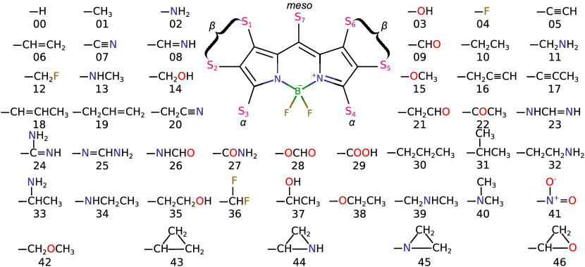
Figure 1: Composition of the BODIPY chemical space studied in this work. In the parent BODIPY molecule all 7 carbon sites, S₁–S₇, are with H. Derivatives are obtained by combinatorially replacing H with 46 substituents.

Even though the earliest report on their synthesis dates as far back as 1968Treibs and Kreuzer (1968), systematic explorations of BODIPYs became popular only in the 1990’sBanuelos (2016); Ulrich et al. (2008). However, the synthesis of unsubstituted BODIPY is relatively recentArroyo et al. (2009); Schmitt et al. (2009). Advances in reaction methodologies and regioselective synthesis protocols have enabled targeted design of BODIPYsShimada et al. (2020); Feng et al. (2016); Chen et al. (2009); Wang et al. (2013a). Systematic chemical mutations of BODIPY and their effects on the electronic spectra provided insights towards rational compound designDonnelly et al. (2020); Tao et al. (2019); Lu et al. (2014). As for their photochemical properties, substitution at the meso position was found to offer significant controlDonnelly et al. (2020); Prlj et al. (2016). While this collective experimental knowledge on BODIPYs represents the ground reality of their electronic structure, there are known gaps in the chemical trends stemming from chemists’ bias and synthetic limitations. In the case of organic photovoltaic materials, high-throughput quantum chemistry combined with artificial intelligence algorithms has provided a bias-free solution for better characterizationHachmann et al. (2011).

Among quantum chemistry approaches for excited state modeling, those revered for their favorable speed includes equation of motion coupled cluster with singles and doubles, EOM-CCSD, approximate CCSD, CC2Christiansen et al. (1995), and algebraic diagrammatic construction method in second-order perturbation theoryDreuw and Wormit (2015). Techniques like spin-component-scaling and scaled-opposite-spin improve all three approachesTajti et al. (2019). Their approximated versions such as resolution-of-identity CC2, RI-CC2Hättig and Weigend (2000); Send et al. (2011), and local pseudo natural orbital similarity transformed EOM-CCSD, DLPNO-STEOM-CCSDBerraud-Pache et al. (2020), retain the accuracy while decreasing their computational scaling by an order. RI-CC2 has been used previously for generating excited state spectra of a chemical space dataset with 22,780 small organic moleculesRamakrishnan et al. (2015a). For larger molecules, especially for high-throughput Big Data generation, the scaling offered by the aforementioned wavefunction methods are still unfavorable rendering time-dependent density functional theory, TDDFT Gross and Maitra (2012); Runge and Gross (1984) as the preferred choice.

Quantum machine learning (QML) methodsRupp et al. (2012); Ramakrishnan and von Lilienfeld (2017); von Lilienfeld (2018) have come a long way from being tools for data analysis to be regarded as the ‘catalyst’ in quantum chemistry big data campaignsHachmann et al. (2011); Ramakrishnan et al. (2015b); Lopez et al. (2016); Beard et al. (2019); Abreha et al. (2019). State-of-the-art structural descriptors facilitate inductive modeling of ground state properties with prediction accuracies better than that of modern DFT approximationsRamakrishnan and von Lilienfeld (2017); Goscinski et al. (2021). For excited state properties, in general, the error rates in QML have been noted to be inferior compared to that of ground state propertiesFaber et al. (2018); Ye et al. (2020); Liu et al. (2021); Mazouin et al. (2021). Yet, QML methods continue to find applications in excited state modeling in chemical space datasetsRamakrishnan et al. (2015a); Tapavicza et al. (2021); Çaylak et al. (2019); Çaylak and Baumeier (2021) as well as in potential surface manifoldsWestermayr and Marquetand (2020a); Häse et al. (2020); Koerstz et al. (2021); Ju et al. (2021); Kiyohara et al. (2020); Westermayr and Marquetand (2020b). Keeping abreast with the progress in QML, materials/molecules inverse-design protocols have also advanced since the earliest implementation nearly twenty years agoFranceschetti and Zunger (1999). Wang et al.Wang et al. (2013b) employed the extreme ML neural network with descriptors of varying rigour to predict experimental excitation properties of selected BODIPYs. Huwig et al.Huwig et al. (2017) inverse-designed benzene derivatives with different properties preferred for dye-sensitized solar cell applications. Recently, Lu et al.Lu et al. (2021) inverse designed BODIPY dyes, for applications in dye-sensitized solar cells.

In the present study, we enumerate the complete chemical space formed by combinatorially introducing 46 small organic groups with up to 3 CONF atoms at all free sites of BODIPY. We generate geometries of all possible singly and doubly substituted BODIPYs, and randomly drawn subsets with triple-to-septuple substitutions. For the resulting set of 77,412 molecules, we obtain accurate DFT-level geometries and determine excited state properties with TDDFT. We perform detailed chemical analyses on the functional group modulation of the lowest excitation energy corresponding to the brightest state. The dataset generated is used to benchmark the performance of a kernel-based QML approaches for modeling excitation energies with various molecular descriptors. Using the best model as a property generator, we embark on inverse-designing BODIPY molecules with target excitation energies.

II Data and Methods

II.1 BODIPYs Chemical Space Design

The size of the BODIPY chemical space formed by combinatorially introducing functional groups at all the free sites is countably infinite. A suitable molecular subspace may be identified by limiting the size of these functional groups. While BODIPYs with varied Stokes shifts for multicolor fluorescence microscopy have been developedBittel et al. (2018), most exhibit only modest shifts suggesting the excited-state geometries to be very similar to that in the ground-stateLoudet and Burgess (2007); Ziessel et al. (2007). Hence, it is sufficient to model only the vertical excitation energies of BODIPYs without adiabatic considerations. To this end, we select a set of 46 small organic substituents and combinatorially introduce them at the 7 free sites of BODIPY (two $\alpha$: sites-3,4, four $\beta$: sites-1,6, sites-2,5, and one: meso: site-7), as presented in FIG. 1. Further, we explore only those derivatives formed by single-bond connectivities and avoid substituents leading to fused rings. To keep the substituents devoid of chemists’ bias, we sampled them from the smallest molecules of the QM9 databaseRamakrishnan et al. (2014). Some functional groups missing in the QM9 molecules have been introduced for the sake of completeness providing groups spanning a spectrum of electron-donating/electron-withdrawing capacity.

Table 1: Size of the BODIPY chemical space considered in this study. The numbers correspond to unique molecules formed by replacing out of 7 H atoms in BODIPY with $N_{s}$ substituents listed in FIG. 1. The enumeration was performed algebraically. Numbers in parentheses correspond to molecules for which coordinates were generated for DFT and QML modeling.

$N_{s}$		Unique molecules
0		1	(1)
1		184	(184)
2		22,287	(22,287)
3		1,706,554	(10,999)
4		78,358,654	(10,990)
5		2,162,757,252	(10,982)
6		33,160,087,804	(10,986)
7		217,911,067,336	(10,983)
Total		253,314,000,072	(77,412)

On an asymmetric framework, the total number of molecules that can be formed by introducing 46 groups in 7 sites should be $46^{7}=435.8\times 10^{9}$. However, since the unsubstituted BODIPY framework has the C_2v point group symmetryPogonin et al. (2020); Teets et al. (2009), this number drops when redundant entries are eliminated. For such symmetry constrained enumerations, PólyaPólya (1937); Freudenstein (1967); Polya and Read (2012) has suggested an algebraic strategy that has been used for non-constructive enumeration of chemical compound spacesChakraborty et al. (2019). With in the constraints of C_2v, the total number of molecules in the BODIPYs chemical space considered here amounts to $253\times 10^{9}$, as reported in Table. 1. We selected all compounds with up to 2 substitutions (22,472 molecules) and 11,000 entries with 3–7 substitutions. In the latter categories 60 molecules exhibited poor convergence in DFT calculations and were discarded. The resulting set of 77,412 unique BODIPY molecules were utilized for training QML models.

II.2 Quantum Chemistry

Initial geometries of 77,412 BODIPY molecules were generated by the “lego approach”—three dimensional structures of substituents attached to the BODIPY sites. These geometries were relaxed using the universal force field (UFF)Rappé et al. (1992) as implemented in OpenbabelO’Boyle et al. (2011). Subsequently, these geometries were relaxed with the semi-empirical method, PM7Stewart (2013) available in MOPAC2016MOP (2016). Finally, the geometries were optimized to their minimum energy configurations at the B3LYP levelBecke (1993) with the Weigend basis set, def2-SVP. B3LYP calcuations were accelerated with RIVahtras et al. (1993); Kendall and Früchtl (1997) using the Weigend auxiliary basis setsWeigend (2006), as implemented in TURBOMOLEFurche et al. (2014). At the TDDFT level, CAM-B3LYPYanai et al. (2004)/def2-TZVP, we calculated the lowest ten excited states of all 77,412 molecules in a single-points fashion using the B3LYP/def2-SVP geometries. TDDFT calculations were accelerated by RIJCOSX, RI approximation for Coulomb (J) and ‘Chain-Of-Spheres’ (COS) algorithm for exchange integrals, as implemented in ORCANeese (2012).

The performance of long-range corrected hybrid DFT functionals for excited spectra is well-established for diverse benchmark datasetsGoerigk and Grimme (2010). Amongst these, CAM-B3LYPYanai et al. (2004) presents good correlations with experimentalMomeni and Brown (2015), EOM-CCSDBose et al. (2016), and CC2 resultsShao et al. (2019). Thus, for a selected subset of BODIPY derivatives, we benchmarked CAM-B3LYP’s accuracy along with that of BLYPBecke (1988), B3LYPBecke (1993) against STEOM-DLPNO-CCSD methodBerraud-Pache et al. (2020) with the def2-TZVP basis set using ORCA. Additionally, CAM-B3LYP’s performance is also tested against the SOS-CIS(D) methodGrimme and Izgorodina (2004); Rhee and Head-Gordon (2007) with aug-cc-pVDZ basis set using QCHEMShao et al. (2015). The latter wavefunction method is known to exhibit good accuracy for excitation energiesChibani et al. (2014); Bose et al. (2017) with experimental results. Here, we want to compare its performance with STEOM-DLPNO-CCSD for modeling BODIPY’s ${\rm S}_{0}\rightarrow{\rm S}_{1}$ excitation energy.

II.3 Machine Learning

In the present study, we employed the kernel ridge regression (KRR) QML method for its accuracy, scalability, and interpretability marked by successes in various endeavorsHuang and von Lilienfeld (2020); Gupta et al. (2021); Krämer et al. (2020); Faber et al. (2018); Huang et al. (2020); Rupp (2015). For various molecular properties, the learning rates of KRR-QML was shown to improve with increasing training-set sizeRamakrishnan and von Lilienfeld (2015); Huang and von Lilienfeld (2020); Gupta et al. (2021); Krämer et al. (2020); Tapavicza et al. (2021); Faber et al. (2018); Huang et al. (2020). In KRR, property modeling is posed as a regression problem using the ‘kernel trick’, where a higher dimensional feature space is sampled using a kernel function. Hence, the regression problem can be expressed as $\left({\bf K}+\lambda{\bf I}\right){\bf c}={\bf p}$, where ${\bf K}$ is the kernel matrix, $\lambda$ is a hyperparameter quantifying the regularization strength, ${\bf c}$ is the regression coefficient vector, and ${\bf p}$ is the target property vector. The elements of the positive-semi-definite kernel matrix are given by $k_{ij}=k({\bf d}_{i},{\bf d}_{j})\in(0,1]$, where ${\bf d}_{i}$ is the descriptor vector for the $i$-th entry. For the choice of descriptor, we benchmarked the performances of a 1-hot representation along with the structural descriptors: Bag-of-BondsHansen et al. (2015)(BoB), Felix-Christensen-Huang-Lilienfeld (FCHL)Faber et al. (2018), and Spectrum of London and Axilrod-Teller-Muto potential (SLATM)Huang and von Lilienfeld (2020). SLATM and FCHL descriptors were generated using the QML packageChristensen et al. (2017), while BoB and 1-hot vector using an in-house code. The 1-hot representation was shown to perform well when the dataset is combinatorially diverseFaber et al. (2016); Ward et al. (2017); Kayastha and Ramakrishnan (2021); Heinen et al. (2021). The 1-hot representation is a 322-bit ($7\times 46$) vector, where the presence/absence of one of the 46 substituents at the 7 sites is denoted by 1/0. This representation does not include any information on the BODIPY framework that is common to all molecules.

For the choice of kernel function, we used the Laplacian function, $k({\bf d}_{i},{\bf d}_{j})=\exp(-|{\bf d}_{i}-{\bf d}_{j}|_{1}/\sigma)$, where $|\cdot|_{1}$ denotes the L₁ norm while $\sigma$ is the hyperparameter quantifying kernel width. For FCHL, we determined an optimal kernel width of $\sigma=5$ by scanning with a fixed regularization strength along with a cutoff of 5 Å. For selecting hyperparameters, we followed the single-kernel strategyRamakrishnan and von Lilienfeld (2015). When there is no linear dependency in the reproducing kernel Hilbert spaceHo and Rabitz (2003), $\lambda$ can be exactly set to 0.0. To prevent near linear dependency rendering the kernel matrix singular due to finite precision, especially for large training sets, we used a small value of $\lambda=0.001$ throughout, as in our previous work on ML modeling of ¹³C NMR shielding constantsGupta et al. (2021). The kernel width was selected using the sample median of all descriptor differences, $d_{ij}^{\rm median}={\rm median}\{|{\bf d}_{i}-{\bf d}_{j}|_{1}\}$, as $\sigma=d^{\rm median}_{ij}/(\log 2)$Ramakrishnan and von Lilienfeld (2015). For 1-hot/BoB/SLATM representations, the optimal $\sigma$ was found to be 26.57/3603.98/840.09. All structural representations were calculated using PM7 level minimum energy geometries to facilitate rapid querying in the BODIPY chemical space with QML.

II.4 Machine Learning aided Inverse-Design

For inverse-design of BODIPY derivatives with a desired S₀ $\rightarrow$ S₁ excitation energy, we used a trained QML model as a rapid surrogate to DFT. We found the QML model based on the SLATM descriptor to deliver best learning rates as discussed later in Section III.2. For minimizing molecular configuration variables in the property manifold defined by the QML model, we explored Bayesian optimization and genetic algorithm (GA) operating in the SLATM feature space.

II.4.1 Bayesian optimization

The Bayesian optimization method is self-correctingJones et al. (1998). Its performance improves over iterations by using previously sampled attribute-value (i.e. descriptor-property) pairs as prior. The ‘gradient’ for sampling the next entry is estimated by Gaussian process regressionRasmussen (2003). The process begins with a normally distributed ($\mathcal{N}$) sample space of descriptor vectors of a training set, ${\bf t}=\{t_{1},t_{2},\ldots\}$, along with the corresponding property values, ${\bf p}_{\bf t}=\{p_{t_{1}},p_{t_{2}},\ldots\}$.

$${\bf p}_{\rm t}\thicksim\mathcal{N}({\bf p}_{\rm t},\boldsymbol{\Sigma}_{\bf tt}),$$ (1)

where $\boldsymbol{\Sigma}_{\bf tt}$ is the positive definite covariance matrix, taken as the Gaussian kernel matrix with an added noise. For a set of query molecules, ${\bf q}=\{q_{1},q_{2},\ldots\}$, the target property values and their uncertainties are predicted as the mean and variance of a Normal distribution, ${\bf p}_{\bf q}\thicksim\mathcal{N}(\boldsymbol{\mu_{*}},\boldsymbol{\Sigma_{*}})$. The estimated mean values, $\boldsymbol{\mu_{*}}$ and variances, $\boldsymbol{\Sigma_{*}}$, are given as

$${\bf p}_{\bf q}\thicksim\boldsymbol{\mu_{*}}=\left[\boldsymbol{\Sigma}_{\bf tq}\right]^{\rm T}\left[\boldsymbol{\Sigma}_{\bf tt}\right]^{-1}{\bf p}_{\bf t}.$$ (2)

Prediction variance is given by the diagonal elements of the matrix

$$\boldsymbol{\Sigma_{*}}=\boldsymbol{\Sigma}_{\bf qq}-\left[\boldsymbol{\Sigma}_{\bf tq}\right]^{\rm T}\left[\boldsymbol{\Sigma}_{\bf tt}\right]^{-1}\boldsymbol{\Sigma}_{\bf tq}.$$ (3)

Hence, the predicted property for a query is the $q$-th element of $\boldsymbol{\mu_{*}}$, $\mu_{q}$. The corresponding variance, $\sigma_{q}$, is the diagonal element of $\boldsymbol{\Sigma}_{\bf qq}$ at row-$q$ and column-$q$. New sampling points are proposed using an acquisition function, $\mathcal{A}$. A popular choice for $\mathcal{A}$ is the expected improvement defined as

$$\mathcal{A}(q)=\begin{cases}Z_{q}\Phi(-\frac{Z_{q}}{\sigma_{q}})+\sigma_{q}\phi(-\frac{Z_{q}}{\sigma_{q}}),&\text{if }\sigma_{q}>0\\ 0,&\text{if }\sigma_{q}=0\end{cases}$$ (4)

where $Z_{q}=\mu_{q}-{\rm max}(\{\boldsymbol{\mu_{*}}\})+\zeta$, the set $\{\boldsymbol{\mu_{*}}\}$ contains all values sampled until a given iteration, and $\zeta$ is a real-valued hyper-parameter, while $\Phi$ and $\phi$ are the cumulative and probability distribution functions of $\mathcal{N}$, respectively.

II.4.2 Genetic Algorithm

Genetic algorithm (GA) is an evolution-inspired heuristic method for optimization in a high-dimensional space with combinatorially coupled variablesWhitley (1994). For sampling in chemical space, GA has been shown to be a suitable frameworkBrowning et al. (2017); Verhellen and Van den Abeele (2020). In this study, we initialized the first generation in GA optimization with a population of 20 random molecules, and a mutation rate of 0.01. Additionally, in each generation, we populated the sample with 10 random molecules. For the entire sample, $E({\rm S}_{0}\rightarrow{\rm S}_{1})$ was predicted by an ML model trained on DFT-level properties. Absolute deviation of these energies from the target value was used as the fitness, and only molecules with deviations smaller than the population median entered subsequent generations through crossover. Our implementation of the Bayesian and GA optimizations along with sample input files and details of control parameters are available at https://github.com/moldis-group/bodipy.

III Results and Discussion

III.1 Chemical trends in ${\rm S}_{0}\rightarrow{\rm S}_{1}$ excitation energy

Wavelength tuning of BODIPY by controlled synthesis has been successful for a handful of symmetrically substituted derivativesLu et al. (2014).

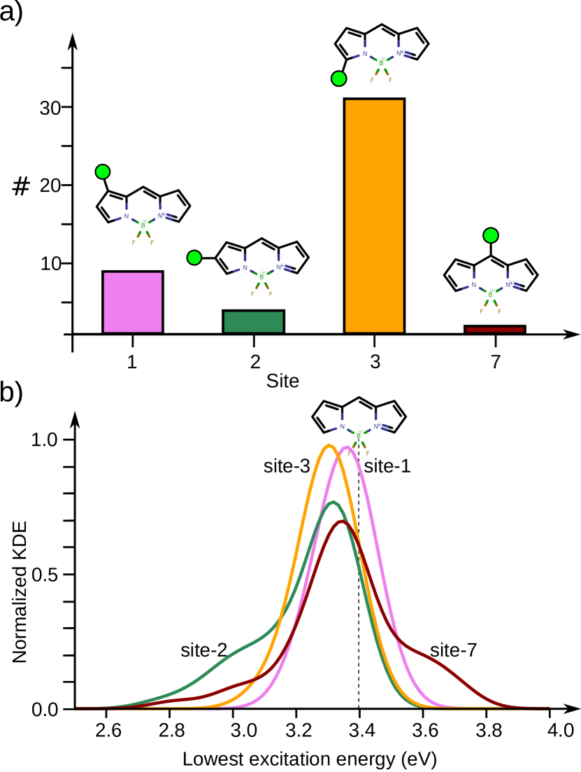
Figure 2: Site-specific statistics for singly-substituted BODIPYs. a) Frequencies of thermodynamically most preferred site for 46 substituents. b) Distribution of S${}_{0}\rightarrow$S₁ excitation energies for 46 singly-substituted BODIPY molecules per site. Vertical dashed line marks the value for unsubstituted BODIPY.

A more comprehensive picture of the dependence of the wavelength shift, corresponding to the brightest excitation, on chemical factors requires further evidences sampled across a larger chemical space. Herein, we investigate the roles played by the substitution sites and the groups in modulating BODIPY’s stability and excitation characteristics.

To identify a suitable level of DFT approximation, for high-throughput modeling, we benchmarked the ${\rm S}_{0}\rightarrow{\rm S}_{1}$ excitation energies of the unsubstituted BODIPY and 184 of its singly-substituted derivatives. For references, we used STEOM-DLPNO-CCSD/def2-TZVP and SOS-CIS(D)/aug-cc-pVDZ results. Five singly substituted derivatives failed to converge at the reference wavefunction-level calculations and these were not included for benchmarking. Compared to STEOM-DLPNO-CCSD/def2-TZVP we obtained mean absolute errors (MAEs) of 0.31$\pm$0.33/0.13$\pm$0.16/0.05$\pm$0.06 eV for BLYP/B3LYP/CAM-B3LYP DFT methods with the def2-TZVP basis set. CAM-B3LYP values were also found to agree with the SOS-CIS(D)/aug-cc-pVDZ level yielding an MAE of 0.05$\pm$0.05 eV. Hence, we performed all TDDFT calculations at the CAM-B3LYP/def2-TZVP level. Even though the SOS-CIS(D) and the STEOM-DLPNO-CCSD calculations have been performed with different basis sets, they agree well with a coefficient-of-correlation ($R^{2}$) of 0.82 and an average deviation of 0.04$\pm$0.05 eV. Hence, we conclude the residual errors in CAM-B3LYP/def2-TZVP based excited state results of the BODIPYs dataset presented here to be with in the uncertainties expected across wavefunction methods and basis set definitions.

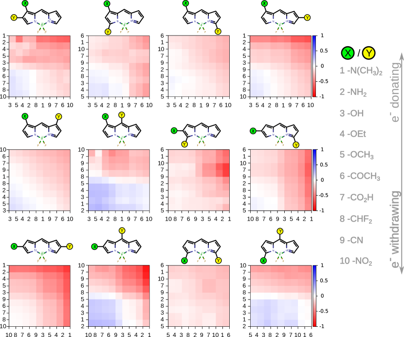
Figure 3: Modulation of S${}_{0}\rightarrow$S₁ excitation energy with substitution. For 12 unique double substitution patterns, shifts in excitation energy, $\Delta E=E{\rm(substituted)}-E{\rm(BODIPY)}$, are presented. For clarity, only 10 substituents that are a standard scale of electron-donating/-withdrawing are drawn from the 46-set shown in FIG 1. In each of the 12 panels, X and Y ordering is according to shifts in singly-substituted compounds.

Table 2: Error metrics for a group-additive estimation of the lowest excitation energy with respect to actual TDDFT values for multiply substituted BODIPY molecules: mean absolute error (MAE in eV), standard deviation (SD in eV), mean percentage absolute error (MPAE), and coefficient of determination ($R^{2}$) are presented.

Substitution	MAE	SD	MPAE	$R^{2}$
doubles	0.03	0.06	1.07	0.87
triples	0.06	0.09	2.09	0.76
quadruples	0.10	0.13	3.33	0.62
quintuples	0.14	0.15	4.69	0.49
hextuples	0.19	0.19	6.38	0.20
septuples	0.24	0.21	8.12	-0.01

In FIG. 2a, we present the frequencies of the thermodynamically favored site for all 46 substituents. This qualitative trend will be reflected in their relative synthetic yields at the high-temperature limit. We find site-3 to be preferred by most groups, as previously noted for alkyl-based substituentsMukherjee and Thilagar (2015), followed by site-1. Accommodating the substituents in both sites (1 & 3) result in minimal perturbation of the TDDFT excitation energy of BODIPY scaffold at 3.40 eV, see FIG. 2b. This value deviates by 0.91 eV from the more reliable STEOM-DLPNO-CCSD value of 2.49 eV. The latter, is in excellent agreement with the experimental value $\lambda_{\rm max}^{\rm abs.}=503$ nm (2.46 eV) and $\lambda_{\rm max}^{\rm em.}=512$ nm (2.42 eV)Schmitt et al. (2009).

A small systematic red shift of the site-3 values maybe ascribed to the non-bonding interactions between the groups and an F atom of BODIPY. Site-2 ($\beta$) and site-7 (meso), that are thermodynamically least preferred also result in strong shifts of the S${}_{0}\rightarrow$S₁ excitation energy, FIG. 2b. Of particular interest, substitutions at site-2 mostly red-shifts the base excitation energy of BODIPY while that at site-7 results in blue-shifting. Chemical non-equivalence of site-2 compared to the other sites has been rationalized by the presence of a node in the lowest unoccupied molecular orbital (LUMO)Lu et al. (2014). The most blue-shifting substituent/site combination corresponds to ethylamine at site-7 (excitation energy at 3.70 eV), while the most red-shifting one is dimethylamine at site-2 (excitation energy at 2.78 eV). It is interesting to note that both ethylamine and dimethylamine are groups with similar electron-donating capacity. Hence, at least for the case of singly substituted BODIPY derivatives, thermodynamic stabilities and the shift of excitation energy are largely controlled by the substitution site.

The singly substituted BODIPY derivatives show substitution on site 7 to provide the most versatile tuning followed by sites 2/5, 3/4, and 1/6. However, it does not disclose ‘inter-substituent’ interactions affecting the overall excitation properties. To gauge the exact nature and extent of these inter-substituent interactions, we inspect the deviation of the TDDFT value of $E_{\mathrm{S}_{0}\rightarrow\mathrm{S}_{1}}$ of an $n$-tuply substituted BODIPY derivative from that of values estimated by employing additivity principle

$$E_{\mathrm{S}_{0}\rightarrow\mathrm{S}_{1}}= E_{\mathrm{S}_{0}\rightarrow\mathrm{S}_{1}}^{\rm BODIPY}+\Delta E_{n}(s_{1}^{g_{1}},\ldots,s_{n}^{g_{n}}).$$ (5)

Here, $E_{\mathrm{S}_{0}\rightarrow\mathrm{S}_{1}}$ is the first excitation energy of a BODIPY derivative, $E_{\mathrm{S}_{0}\rightarrow\mathrm{S}_{1}}^{\rm BODIPY}$ being the value corresponding to the unsubstituted BODIPY. For a singly-substituted derivative with group $1\leq g_{1}\leq 46$ at site $1\leq s_{1}\leq 7$, an exact shift, $\Delta E_{1}(s_{1}^{g_{1}})$, is calculated as the difference between the singly-substituted and unsubstituted BODIPYs.

For Eq. 5 to be of practical use in estimating the energy of an arbitrary derivative, the higher-order corrections should be approximated by lower-order terms. Here, we use $\Delta E_{1}(s_{1}^{g_{1}})$ determined for the singly-substituted derivatives to approximate the higher-order terms as the sum

$$\Delta E_{n}(s_{1}^{g_{1}},\ldots,s_{n}^{g_{n}})\approx\sum_{k=1}^{n}\Delta E_{1}(s_{k}^{g_{k}}).$$ (6)

In Table. 2, we present the statistics for the estimation of TDDFT excitation energies of 77 k BODIPYs, for exact counts of molecules, see Table. 1. The estimated values of 22 k doubly substituted ($n=2$) derivatives show a good agreement with the target TDDFT values with a mean absolute error (MAE) of 0.03 eV and a Spearman rank correlation ($\rho$) of 0.95, see Table 2.

The agreement between the reference values and the additivity model diminishes with increase in the number of substituents. For every additional substituent, the increase in error is 0.03–0.04 eV. A similar increase in the standard deviation suggest the errors to have non-systematic contributions. For the limiting case, $n=7$, the prediction MAE is $>0.2$ eV—over $8\%$ of the reference values—which is comparable to the spread of excitation energy values. Furthermore, the $R^{2}$ value for estimations was found to be essentially zero. Since a large fraction of the BODIPYs chemical space comprises of septuply-substituted molecules, such large errors make group additive estimation a poor baseline for $\Delta-$QMLRamakrishnan et al. (2015b). While systematic diagnostics to quantify a method as a baseline is still lacking, in our past $\Delta-$QML works, we found better learning rates when $R^{2}>0.5$ when comparing the baseline and targetline values. In $\Delta-$QML modeling of DFT-level ¹³C NMR shielding of QM9 molecules, a minimal basis set baseline yielded $R^{2}=0.66$ resulting in better learning rates than modeling directly on the target valuesGupta et al. (2021).

Upon double substitution, we note the range of S${}_{0}\rightarrow$S₁ excitation to increase compared to the singly substituted compounds. While the majority of BODIPYs show red-shifted $\lambda_{\rm max}$, compared to the unsubstituted molecule, combinatorial exploration with high-throughput first-principles calculations identifies a non-negligible fraction of blue-shifted molecules. Out of 22,287 doubly-substituted BODIPYs studied here, 95.45% corresponding to 21,272 entries have large S${}_{0}\rightarrow$S₁ oscillator strengths ($f>0.5$) suggesting good potential for light-harvesting applications. However, only 1,884 of these candidates were found to be blue-shifted. The increase in the approximation error in Eq.6, with increasing $n$ may be expected as the joint chemical effects due to multiple substituents can no longer be treated as a weak perturbations. We inspect the $n=2$ case corresponding to the excitation energies of 22,287 doubly substituted BODIPYs to identify the combinations of sites/groups resulting in non-additive trends. For this purpose, we selected 10 representative substituents (out of 46) with well-characterized electron-donating and withdrawing abilities compared to the standard aromatic molecule, benzene.

FIG. 3 presents the shift in $E({\rm S}_{0}\rightarrow{\rm S}_{1})$ across 12 positional isomers of doubly substituted BODIPY derivatives with respect to unsubstituted BODIPY. The order of X and Y axes are independently sorted according to the shifts in the singly-substituted series. Hence, in FIG. 3, for the first heatmap (top, left-most), at site 1 we have X substituents along the X-axis while the substituents at site 2 have Y substituents on Y-axis. In the selected color scale, the blue-shifted molecules will appear blue while the red-shifted entries appear in red. For symmetric combinations of sites, where (X,Y) = (1,6), (2,5), and (3,4), the number of unique molecules is 55—for consistency, these heatmaps are presented by duplicating entries. The group additivity model (Eq. 6) does not differentiate positional isomers. For instance, since site-2 and site-5 are equivalent for single substitution, for the combination (1,2) and (1,5) the additivity model will predict same shifts of the excitation energy. Since sites 1 and 5 are spatially separated, the additivity assumption holds better resulting in a smooth transition in the heatmap. However, for (1,2) double substitutions, the effect of inter-substituent interaction is reflected in irregularities in the diagonal gradient (from left/bottom to right/top). Similar trend holds for the (2,3)-vs.-(2,4) case. Substitutions at sites 1 & 3 result in mild shifts as seen in FIG. 3. Hence, (1,4)-derivatives (with weak inter-substituent interactions) yield weak shifts compared to isomerically equivalent (1,3) substitutions.

Blue-shifting of the absorption spectra due to meso substitution (at site-7) was previously observedBañuelos et al. (2011). In FIG. 2, we see this effect for the singly-substituted derivatives. Hence, out of 12 unique doubly substituted patterns, blue-shifting is predominantly noted for three combinations involving site-7: (1,7), (2,7), and (3,7). Of these, since substitutions at sites 1 & 3 result in weak perturbations of BODIPY’s excitation characteristics, a larger fraction of blue-shifted derivatives are seen for (1,7) and (3,7) substitutions. Since single substitutions at sites 2 & 7 have shown strong but contrasting trends, see FIG. 2, their joint occurrence shows constructive and destructive effects. Of the two weakly perturbing sites, 1 & 3, the former results in a slightly blue-shifted distribution, while the latter in a slightly red-shifted distribution, see FIG. 2b. The dependence of the shift with electron donating/withdrawing ability of substituents is similar for sites 1, 3, & 7. Hence, to blue-shift BODIPY, having electron donating groups at sites (1,7) is ideal. Similarly, to red-shift BODIPY, having an electron donating group at 2, and an electron withdrawing group at 3 or 4 is ideal. In FIG. 3, we see the (2,3) combination to benefit from inter-substituent interactions over the (2,4) combination. We tested the validity of these trends by identifying the extreme doubly-substituted molecules by considering the entire set of 46 substituents. The excitation energy of the most blue-shifted derivative appears at 3.84 eV (–OH at site 1 and –NHCH₃ at site 7), while the most red-shifted appears at 2.32 eV (–NHCH₂CH₃ at site 2 and –COCH₃ at site 3).

III.2 Quantum Machine Learning Models

The main objective of QML modeling is to provide an inexpensive inference approach to replace rigorous, first-principles modeling. For reliable high-throughput screening in the BODIPY chemical space, one cannot depend on an additivity model based on chemical effects imparted by site-specific individual substitutions on BODIPY. With increasing substitutions, the additivity model ceases to be even qualitatively accurate, see Table. 2. On the other hand, QML models when sufficiently trained using a baseline geometry can facilitate rapid querying in the uncharted regions across the chemical space. Hence, QML offers an opportunity to effortlessly navigate across the vast BODIPY chemical space with quantitative accuracy. As discussed before (see Sec. II.2), of the 77,412 molecules for which DFT calculations were performed, QML modeling was done with 76,212 entries in the training set. The unsubstituted, and all 184 singly-substituted molecules were kept in training. Of the 22,287 doubly substituted derivatives, 200 was kept in a hold-out set.

Table 3: Breakdown of ML errors for predicting the lowest excitation energy of 1200 hold-out BODIPY derivatives. Mean percentage absolute error (MPAE) is given separately for 200 entries with $N_{s}$ substituents.

$N$		MPAE for various $N_{s}$
		SLATM							1-hot
		2	3	4	5	6	7		2	3	4	5	6	7
100		3.72	4.30	4.67	5.58	5.37	6.18		3.59	4.46	4.96	5.87	6.27	7.40
500		2.18	3.33	3.77	4.37	4.68	5.45		2.60	3.08	3.75	3.82	4.60	5.41
1000		1.85	2.81	3.27	3.69	4.36	4.88		1.71	2.48	2.69	3.04	3.93	4.45
2500		1.36	2.27	2.76	3.22	3.89	4.47		1.23	1.83	2.25	2.68	3.48	3.89
5000		1.11	1.82	2.29	2.81	3.32	3.93		1.04	1.62	2.20	2.60	3.32	3.80
7500		0.96	1.59	2.11	2.85	3.00	3.50		1.02	1.53	2.13	2.58	3.28	3.86
10000		0.83	1.51	2.11	2.66	2.83	3.37		1.01	1.53	2.09	2.53	3.31	3.76
25000		0.68	1.19	1.75	2.35	2.70	2.91		0.92	1.41	2.01	2.48	3.26	3.50
50000		0.51	1.08	1.54	2.04	2.37	2.80		0.84	1.26	1.79	2.56	3.00	3.05
75000		0.48	0.98	1.35	1.93	2.22	2.63		0.76	1.12	1.70	2.41	2.60	3.09

For 11 k molecules with 3–7 substitutions (see Table 1), randomly drawn 200 from each set, was added to the hold-out set amounting to 1,200 molecules. We benchmarked the performance of KRR-QML models using hold-out errors across four different representations: 1-hot, BoB, FCHL and SLATM.

In FIG. 4, we present the performance of QML models. When increasing the training set size to 75 k, all models show essentially monotonous convergence upon validating on a 1,200 hold-out set. Of the four representations, SLATM shows the best performance at the 75 k limit with a mean percentage absolute error (MPAE) of 1.6%. For a conventional dye such as Nile Red, with $\lambda_{max}$ corresponding to 2.41 eVZuehlsdorff and Isborn (2019), this MPAE translates to an uncertainty of $<0.05$ eV, which is well within the uncertainty of the target TDDFT method. The 1-hot, FCHL and BoB representations converge to MPAEs in the 1.9–2.1% range. Compared to the structural representations, the remarkable accuracy of the composition-based representation, 1-hot, may be ascribed to the significant influence of substituent type and site on the overall BODIPY excitation energies rather than three-dimensional structural information. Similar observation has been made in past worksFaber et al. (2016); Ward et al. (2017); Kayastha and Ramakrishnan (2021); Heinen et al. (2021). In the following, we use the best performing SLATM-KRR-QML model.

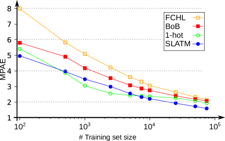
Figure 4: Learning rates for KRR-QML models based on the structure-based descriptors—FCHL, BoB, and SLATM—and a composition-based 1-hot representation. Mean percentage absolute error (MPAE) for predicting TDDFT-level ${\rm S}_{0}\rightarrow{\rm S}_{1}$ excitation energies of 1,200 hold-out BODIPY derivatives is shown for varying training set sizes.

Although the MPAE for the 1,200 hold-out set indicates the QML models to provide accurate results in agreement with 1-hot-KRR-QML models calculated separately for 200 entries from each subset with 2–7 substitutions. In all categories, both representations converge to small MPAEs with increasing model size, with SLATM delivering better results. Both models provide least errors for doubly substituted derivatives while the worst results are noted for septuply substituted ones. The reason for the deterioration of the models’ performance with increasing number of substituents is because highly substituted derivatives are under-represented in the training set. However, it must be noted for the most diverse case of septuply substituted BODIPYs, SLATM and 1-hot based models delivered MPAEs of 2.63 and 3.09% despite using only 0.0000296% of the total space.Hence, we conclude SLATM-KRR-QML and 1-hot-KRR-QML models to be rapid and accurate alternatives for first-principles high-throughput modeling. Further, by exploiting the excellent QML cost to accuracy trade-off we demonstrate the applicability of the 1-hot-KRR-QML model in the form of a publicly accessible web interface for navigating the chemical space of BODIPYs with 253 giga molecules, see Appendix.

Figure 5: Convergence of inverse design searches of BODIPY molecules with ${\rm S}_{0}\rightarrow{\rm S}_{1}$ excitation energy targets: 2.8 eV, 3.0 eV, and 3.2 eV: a) Comparison of unconstrained Bayesian optimization and genetic algorithm (GA). In each case, the final, optimal solutions are shown. b) Bayesian search was performed separately in doubly substituted (2D) and septuply substituted (7D) subspaces. Gray region marks the first 5 iterations for building a Gaussian process model. Navigation trajectories start from the unsubstituted BODIPY (3.40 eV). Intermediate solutions are also shown. The target property was calculated using a SLATM-KRR-QML model, trained on TDDFT data for 75,000 examples. To accelerate predictions, PM7 level geometries were used for generating the SLATM descriptor. Python codes for inverse design are maintained at https://github.com/moldis-group/DesignBODIPY.

III.3 Inverse designing BODIPY derivatives

Inverse design offers a very economic solution to zero-in on molecules with desirable properties because the solution is sought iteratively without having to screen through all possibilities in an Edisonian approach. Inverse design is a mathematically ill-posed problem due to a surjective (i.e., many-to-one) mapping between the chemical structure and the target property. However, when the target property value is known to correspond to one or many solutions, state-of-the-art algorithms provide optimal solutions with in a numerical precision. Here, we explore the possibility to inverse design BODIPY derivatives with fixed ${\rm S}_{0}\rightarrow{\rm S}_{1}$ excitation energy targets. The function values (property) required for the inverse design optimizers can ideally come from TDDFT calculations albeit at a higher computational overhead. Hence, we use the SLATM-KRR-QML model to estimate the property because of favorable accuracy-vs-speed.

While it may be desired for inverse design to search for systems with extreme property values, its performance is dependent on the knowledge included in the property generator. Our models were trained on a randomly drawn subset of the total chemical space. Most molecular properties result in peaked distributions with sparsely populated tails. Hence, molecules at these extreme regions of the distributions will be under-represented in any randomly sampled training set. This suggests inverse design based on QML to be less reliable for identifying errors when the target property is in a region of space that is under-represented in the training set, namely the extremes. Hence, it is recommended to perform inverse design for targets belonging to regions in the property space that was adequately represented in the training set for a QML based property-generator. Here, we investigate the applicability of QML guided inverse design via two commonly used optimization protocols—the Bayesian Optimization and Genetic Algorithm (GA).

In FIG. 5a, we note the performance of unconstrained searches across the BODIPY chemical space. Our targets 2.8 eV, 3.0 eV, and 3.2 eV are all red-shifted compared to the unsubstituted BODIPY, and sufficiently represented in the training set. The prevalence of septuply substituted BODIPY molecules as targets could be expected, as it comprises the largest BODIPY sub-space (see Table. 1). GA requires 20 seeds (not shown in FIG. 5) to pre-condition the optimizer. Hence, for Bayesian optimization, we arrive at BODIPY molecules with target S${}_{0}\rightarrow$S₁ values in fewer iterations than that in GA. Also in Bayesian optimization, only those iterations are considered for which the loss function, (target - predicted)², is greater than the value from the previous iteration. While all searches concluded in septuply substituted BODIPYs for both Bayesian search and GA, it is likely that there are derivatives with $<$ 7 substitutions satisfying the same design target. Hence, this warrants a constrained search in BODIPY sub-spaces where GA will be particularly challenging. Hence, the Bayesian approach is ideal for a constrained inverse design. In the doubly substituted subspace, the candidate structure with a target property value of 2.8 eV, corresponds to a (2,5) derivative. This seem to be in accord with the trend that these sites favor red-shifting. However, rationalization of the intermediate and final solutions in evolutionary searches need not exhibit continuous or known trends because of the very nature of these inverse optimizations exploiting the surjective structure-property mappingHornby et al. (2006). Hence, in inverse design, an attempt to interpret the final optimal solutions is prone to post hoc fallacy.

IV Conclusions

Quantum chemistry aided rational design of a dye molecule guides chemists to identify molecules with favorable excitation properties. Accurate descriptions of excited state characteristics calls for long-range corrected DFT level modeling or beyond. However, the traditional one molecule at-a-time paradigm becomes prohibitively expensive when navigating the BODIPY chemical space formed by systematic introduction of 46 small organic substituents at 7 sites through single bond connectivities, yielding $>253$ Billion molecules.

In this study, we have enumerated the complete chemical space spanned by BODIPYs with various degrees of substitution. For statistical modeling, we sampled 77,412 derivatives from the entire chemical space. The resulting BODIPYs dataset contains, the unsubstituted molecule, all possible singly (184), and doubly substituted (22,287) derivatives along with about 11,000 triply–septuptly substituted derivatives. In the subset comprising singly and doubly substituted derivatives, we identified site-specific chemical trends by screening. Since the BODIPY dyes are known to exhibit small Stokes shifts, the vertical excitation energies provided in this study can aid experimental endeavours. For such attempts to be fruitful, the BODIPYs dataset should be enriched by incorporating systematic corrections through careful calibrations of the TDDFT results presented here using high-level wavefunction theories.

We have presented evidences for the failure of an additivity model to estimate the shift in BODIPY’s excitation energy due to various substitutions. Hence, investigating the complete chemical space of BODIPY with $>$ 2 substituents presents a significant computational challenge. To this end, we benchmarked the performance of KRR-QML models for inductive modeling of the lowest excitation energy. Using DFT-level properties of 77 k example molecules for training the QML model, we compared the performance of three structural representations: SLATM, FCHL, and BoB, and a categorical 1-hot descriptor. QML model trained on 75 k BODIPY entries with the SLATM descriptor exhibits the best performance with an average error of $<2\%$ for a randomly drawn hold-out set. The 1-hot representation, that can be instantaneously generated, delivers the next best performance enabling the development of a publicly accessible web-based QML model enabling rapid and seamless query on the entire chemical space of BODIPY. Using excitation energies predicted by a SLATM-KRR-QML model, we inverse designed BODIPYs with target property values. We tested Bayesian optimization and GA and found the former to outperform the latter. Furthermore, with in the chemical subspaces for a given number of substituents, constrained Bayesian optimization was performed to identify BODIPY molecules exhibiting target excitation energy values.

V Data Availability

PM7, DFT and TDDFT level properties of 77,412 molecules used for training a QML model are available at https://moldis-group.github.io/BODIPYs. A QML model to predict S₀$\rightarrow$S₁ excitation energy of BODIPYs accessible via a web browser is available at https://moldis.tifrh.res.in/db/bodipy.

VI Acknowledgments

We acknowledge support of the Department of Atomic Energy, Government of India, under Project Identification No. RTI 4007. All calculations have been performed using the Helios computer cluster, which is an integral part of the MolDis Big Data facility, TIFR Hyderabad (http://moldis.tifrh.res.in).

*

Appendix A Navigating the BODIPY chemical space using a web-based QML model

We provide a web-based interface for a QML model using the 1-hot representation, trained on 75 k BODIPY derivatives, see FIG. 6. The input in the interface can be provided in two ways: 1) using drop-down menus one can select any of the 46 substituents at each of the 7 sites, or 2) to query multiple molecules, one can manually list the indices of substituents at sites 1–7 in the same order. The inputs in FIG. 6a illustrate some of the concepts discussed in the main text. Influence of electron donating/withdrawing groups at site-7 is opposite to that of hosting the same groups at site-2 or site-5. For BODIPY, the ${\rm S}_{0}\rightarrow{\rm S}_{1}$ excitation energy is at 3.40 eV. Compared to this, the single substituted derivative with group-40 at site-7 is blue-shifted to 3.59 eV, see FIG. 6b. While the value for group-41 at the same site is red-shifted to 3.03 eV (FIG. 6b). The red/blue shifting is reversed when these groups are at site-2. Even though site-5 is equivalent to site-2, one notices small deviations when comparing the results for same groups at both sites. This is because the QML model is trained on unique derivatives, hence the accuracy is differently influenced for chemically equivalent combinations.

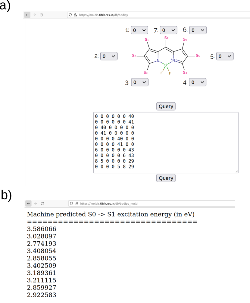
Figure 6: Screenshots of the web-based interface for QML predictions of ${\rm S}_{0}\rightarrow{\rm S}_{1}$ excitation energy in the BODIPY chemical space: a) query page, b) results page. The interface can be accessed at https://moldis.tifrh.res.in/db/bodipy.

References

- Zhang et al. (2013) S. Zhang, T. Wu, J. Fan, Z. Li, N. Jiang, J. Wang, B. Dou, S. Sun, F. Song, and X. Peng, Org. Biomol. Chem. 11, 555 (2013).
- Kowada et al. (2015) T. Kowada, H. Maeda, and K. Kikuchi, Chem. Soc. Rev. 44, 4953 (2015).
- Gómez-Durán et al. (2010) C. A. Gómez-Durán, I. García-Moreno, A. Costela, V. Martin, R. Sastre, J. Bañuelos, F. L. Arbeloa, I. L. Arbeloa, and E. Peña-Cabrera, Chem. Commun. 46, 5103 (2010).
- Umezawa et al. (2008) K. Umezawa, Y. Nakamura, H. Makino, D. Citterio, and K. Suzuki, J. Am. Chem. Soc. 130, 1550 (2008).
- Buyukcakir et al. (2009) O. Buyukcakir, O. A. Bozdemir, S. Kolemen, S. Erbas, and E. U. Akkaya, Org. Lett. 11, 4644 (2009).
- Qi et al. (2020) S. Qi, N. Kwon, Y. Yim, V.-N. Nguyen, and J. Yoon, Chem. Sci. 11, 6479 (2020).
- Ulrich et al. (2008) G. Ulrich, R. Ziessel, and A. Harriman, Angew. Chem. Int. Ed. 47, 1184 (2008).
- Ortiz et al. (2010) M. Ortiz, I. Garcia-Moreno, A. Agarrabeitia, G. Duran-Sampedro, A. Costela, R. Sastre, F. L. Arbeloa, J. B. Prieto, and I. L. Arbeloa, Phys. Chem. Chem. Phys. 12, 7804 (2010).
- Lai and Bard (2003) R. Y. Lai and A. J. Bard, J. Phys. Chem. B 107, 5036 (2003).
- Eçik et al. (2017) E. T. Eçik, E. Özcan, H. Kandemir, I. F. Sengul, and B. Çoşut, Dyes Pigm. 136, 441 (2017).
- Yilmaz et al. (2006) M. D. Yilmaz, O. A. Bozdemir, and E. U. Akkaya, Org. Lett. 8, 2871 (2006).
- Ziessel et al. (2013) R. Ziessel, G. Ulrich, A. Haefele, and A. Harriman, J. Am. Chem. Soc. 135, 11330 (2013).
- Özcan and Çoşut (2018) E. Özcan and B. Çoşut, ChemistrySelect 3, 7940 (2018).
- Bakthavatsalam et al. (2015) S. Bakthavatsalam, A. Sarkar, A. Rakshit, S. Jain, A. Kumar, and A. Datta, Chem. Commun. 51, 2605 (2015).
- Cherumukkil et al. (2018) S. Cherumukkil, B. Vedhanarayanan, G. Das, V. K. Praveen, and A. Ajayaghosh, Bull. Chem. Soc. Jpn. 91, 100 (2018).
- Swamy et al. (2020) P. C. A. Swamy, G. Sivaraman, R. N. Priyanka, S. O. Raja, K. Ponnuvel, J. Shanmugpriya, and A. Gulyani, Coord. Chem. Rev. 411, 213233 (2020).
- Filatov (2020) M. A. Filatov, Org. Biomol. Chem. 18, 10 (2020).
- Awuah and You (2012) S. G. Awuah and Y. You, RSC Adv. 2, 11169 (2012).
- Dahim et al. (2002) M. Dahim, N. K. Mizuno, X.-M. Li, W. E. Momsen, M. M. Momsen, and H. L. Brockman, Biophys. J. 83, 1511 (2002).
- Matsumoto et al. (2007) T. Matsumoto, Y. Urano, T. Shoda, H. Kojima, and T. Nagano, Org. Lett. 9, 3375 (2007).
- Avellanal-Zaballa et al. (2021) E. Avellanal-Zaballa, A. Prieto-Castañeda, C. Díaz-Norambuena, J. Bañuelos, A. R. Agarrabeitia, I. García-Moreno, S. de la Moya, and M. J. Ortiz, Phys. Chem. Chem. Phys. 23, 11191 (2021).
- Ueno et al. (2011) Y. Ueno, J. Jose, A. Loudet, C. Pérez-Bolívar, P. Anzenbacher Jr, and K. Burgess, J. Am. Chem. Soc. 133, 51 (2011).
- Wu et al. (2020) Q. Wu, Z. Kang, Q. Gong, X. Guo, H. Wang, D. Wang, L. Jiao, and E. Hao, Org. Lett. 22, 7513 (2020).
- Kamkaew et al. (2013) A. Kamkaew, S. H. Lim, H. B. Lee, L. V. Kiew, L. Y. Chung, and K. Burgess, Chem. Soc. Rev. 42, 77 (2013).
- Singh and Gayathri (2014) S. P. Singh and T. Gayathri, Eur. J. Org. Chem. 2014, 4689 (2014).
- Kolemen et al. (2011) S. Kolemen, O. A. Bozdemir, Y. Cakmak, G. Barin, S. Erten-Ela, M. Marszalek, J.-H. Yum, S. M. Zakeeruddin, M. K. Nazeeruddin, M. Grätzel, and E. U. Akkaya, Chem. Sci. 2, 949 (2011).
- Erten-Ela et al. (2008) S. Erten-Ela, M. D. Yilmaz, B. Icli, Y. Dede, S. Icli, and E. U. Akkaya, Org. Lett. 10, 3299 (2008).
- Swamy P et al. (2013) C. A. Swamy P, S. Mukherjee, and P. Thilagar, Chem. Commun. 49, 993 (2013).
- Mukherjee and Thilagar (2014) S. Mukherjee and P. Thilagar, Chem. Eur. J. 20, 9052 (2014).
- Nandi et al. (2021) R. P. Nandi, P. Dhanalakshmi, S. K. Behera, and P. Thilagar, Inorg. Chem. 60, 5452 (2021).
- Treibs and Kreuzer (1968) A. Treibs and F.-H. Kreuzer, Justus Liebigs Ann. Chem. 718, 208 (1968).
- Banuelos (2016) J. Banuelos, Chem. Rec. 16, 335 (2016).
- Arroyo et al. (2009) I. J. Arroyo, R. Hu, G. Merino, B. Z. Tang, and E. Pena-Cabrera, J. Org. Chem. 74, 5719 (2009).
- Schmitt et al. (2009) A. Schmitt, B. Hinkeldey, M. Wild, and G. Jung, J. Fluoresc. 19, 755 (2009).
- Shimada et al. (2020) T. Shimada, S. Mori, M. Ishida, and H. Furuta, Beilstein J. Org. Chem. 16, 587 (2020).
- Feng et al. (2016) Z. Feng, L. Jiao, Y. Feng, C. Yu, N. Chen, Y. Wei, X. Mu, and E. Hao, J. Org. Chem. 81, 6281 (2016).
- Chen et al. (2009) J. Chen, M. Mizumura, H. Shinokubo, and A. Osuka, Chem. Eur. J. 15, 5942 (2009).
- Wang et al. (2013a) L. Wang, B. Verbelen, C. Tonnelé, D. Beljonne, R. Lazzaroni, V. Leen, W. Dehaen, and N. Boens, Photochem. Photobiol. Sci. 12, 835 (2013a).
- Donnelly et al. (2020) J. L. Donnelly, D. Offenbartl-Stiegert, J. M. Marin-Beloqui, L. Rizello, G. Battaglia, T. M. Clarke, S. Howorka, and J. D. Wilden, Chem. Eur. J. 26, 863 (2020).
- Tao et al. (2019) J. Tao, D. Sun, L. Sun, Z. Li, B. Fu, J. Liu, L. Zhang, S. Wang, Y. Fang, and H. Xu, Dyes Pigm. 168, 166 (2019).
- Lu et al. (2014) H. Lu, J. Mack, Y. Yang, and Z. Shen, Chem. Soc. Rev. 43, 4778 (2014).
- Prlj et al. (2016) A. Prlj, A. Fabrizio, and C. Corminboeuf, Phys. Chem. Chem. Phys. 18, 32668 (2016).
- Hachmann et al. (2011) J. Hachmann, R. Olivares-Amaya, S. Atahan-Evrenk, C. Amador-Bedolla, R. S. Sánchez-Carrera, A. Gold-Parker, L. Vogt, A. M. Brockway, and A. Aspuru-Guzik, J. Phys. Chem. Lett. 2, 2241 (2011).
- Christiansen et al. (1995) O. Christiansen, H. Koch, and P. Jørgensen, Chem. Phys. Lett. 243, 409 (1995).
- Dreuw and Wormit (2015) A. Dreuw and M. Wormit, WIREs Comput. Mol. Sci. 5, 82 (2015).
- Tajti et al. (2019) A. Tajti, L. Tulipan, and P. G. Szalay, J. Chem. Theory Comput. 16, 468 (2019).
- Hättig and Weigend (2000) C. Hättig and F. Weigend, J. Chem. Phys. 113, 5154 (2000).
- Send et al. (2011) R. Send, M. Kühn, and F. Furche, J. Chem. Theory Comput. 7, 2376 (2011).
- Berraud-Pache et al. (2020) R. Berraud-Pache, F. Neese, G. Bistoni, and R. Izsák, J. Chem. Theory Comput. 16, 564 (2020).
- Ramakrishnan et al. (2015a) R. Ramakrishnan, M. Hartmann, E. Tapavicza, and O. A. von Lilienfeld, J. Chem. Phys. 143, 084111 (2015a).
- Gross and Maitra (2012) E. K. Gross and N. T. Maitra, “Introduction to TDDFT,” in Fundamentals of Time-Dependent Density Functional Theory (Springer, 2012) pp. 53–99.
- Runge and Gross (1984) E. Runge and E. K. Gross, Phys. Rev. Lett. 52, 997 (1984).
- Rupp et al. (2012) M. Rupp, A. Tkatchenko, K.-R. Müller, and O. A. von Lilienfeld, Phys. Rev. Lett. 108, 058301 (2012).
- Ramakrishnan and von Lilienfeld (2017) R. Ramakrishnan and O. A. von Lilienfeld, Rev. Comput. Chem. 30, 225 (2017).
- von Lilienfeld (2018) O. A. von Lilienfeld, Angew. Chem. Int. Ed. 57, 4164 (2018).
- Ramakrishnan et al. (2015b) R. Ramakrishnan, P. O. Dral, M. Rupp, and O. A. von Lilienfeld, J. Chem. Theory Comput. 11, 2087 (2015b).
- Lopez et al. (2016) S. A. Lopez, E. O. Pyzer-Knapp, G. N. Simm, T. Lutzow, K. Li, L. R. Seress, J. Hachmann, and A. Aspuru-Guzik, Sci. 3, 160086 (2016).
- Beard et al. (2019) E. J. Beard, G. Sivaraman, Á. Vázquez-Mayagoitia, V. Vishwanath, and J. M. Cole, Sci. 6, 1 (2019).
- Abreha et al. (2019) B. G. Abreha, S. Agarwal, I. Foster, B. Blaiszik, and S. A. Lopez, J. Phys. Chem. Lett. 10, 6835 (2019).
- Goscinski et al. (2021) A. Goscinski, G. Fraux, G. Imbalzano, and M. Ceriotti, Mach. learn.: Sci. Technol. 2, 025028 (2021).
- Faber et al. (2018) F. A. Faber, A. S. Christensen, B. Huang, and O. A. von Lilienfeld, J. Chem. Phys. 148, 241717 (2018).
- Ye et al. (2020) Z.-R. Ye, I.-S. Huang, Y.-T. Chan, Z.-J. Li, C.-C. Liao, H.-R. Tsai, M.-C. Hsieh, C.-C. Chang, and M.-K. Tsai, RSC Adv. 10, 23834 (2020).
- Liu et al. (2021) Z. Liu, L. Lin, Q. Jia, Z. Cheng, Y. Jiang, Y. Guo, and J. Ma, J. Chem. Inf. Model. 61, 1066 (2021).
- Mazouin et al. (2021) B. Mazouin, A. Alain Schöpfer, and O. A. von Lilienfeld, arXiv preprint arXiv:2110.02596 (2021).
- Tapavicza et al. (2021) E. Tapavicza, G. F. von Rudorff, D. O. De Haan, M. Contin, C. George, M. Riva, and O. A. von Lilienfeld, Environ. Sci. Technol. 55, 8447 (2021).
- Çaylak et al. (2019) O. Çaylak, A. Yaman, and B. Baumeier, J. Chem. Theory Comput. 15, 1777 (2019).
- Çaylak and Baumeier (2021) O. Çaylak and B. Baumeier, J. Chem. Theory Comput. 17, 4891 (2021).
- Westermayr and Marquetand (2020a) J. Westermayr and P. Marquetand, J. Chem. Phys. 153, 154112 (2020a).
- Häse et al. (2020) F. Häse, L. M. Roch, P. Friederich, and A. Aspuru-Guzik, Nat. Commun. 11, 1 (2020).
- Koerstz et al. (2021) M. Koerstz, A. S. Christensen, K. V. Mikkelsen, M. B. Nielsen, and J. H. Jensen, PeerJ Phys. Chem. 3, e16 (2021).
- Ju et al. (2021) C.-W. Ju, H. Bai, B. Li, and R. Liu, J. Chem. Inf. Model. 61, 1053 (2021).
- Kiyohara et al. (2020) S. Kiyohara, M. Tsubaki, and T. Mizoguchi, Npj Comput. Mater. 6, 1 (2020).
- Westermayr and Marquetand (2020b) J. Westermayr and P. Marquetand, Chem. Rev. (2020b).
- Franceschetti and Zunger (1999) A. Franceschetti and A. Zunger, Nature 402, 60 (1999).
- Wang et al. (2013b) J.-N. Wang, J.-L. Jin, Y. Geng, S.-L. Sun, H.-L. Xu, Y.-H. Lu, and Z.-M. Su, J. Comp. Chem. 34, 566 (2013b).
- Huwig et al. (2017) K. Huwig, C. Fan, and M. Springborg, J. Chem. Phys. 147, 234105 (2017).
- Lu et al. (2021) T. Lu, M. Li, Z. Yao, and W. Lu, J. Materiomics 7, 790 (2021).
- Bittel et al. (2018) A. M. Bittel, A. M. Davis, L. Wang, M. A. Nederlof, J. O. Escobedo, R. M. Strongin, and S. L. Gibbs, Sci. Rep. 8, 1 (2018).
- Loudet and Burgess (2007) A. Loudet and K. Burgess, Chem. Rev. 107, 4891 (2007).
- Ziessel et al. (2007) R. Ziessel, G. Ulrich, and A. Harriman, New J. Chem. 31, 496 (2007).
- Ramakrishnan et al. (2014) R. Ramakrishnan, P. O. Dral, M. Rupp, and O. A. von Lilienfeld, Sci. Data 1, 1 (2014).
- Pogonin et al. (2020) A. E. Pogonin, A. Y. Shagurin, M. A. Savenkova, F. Y. Telegin, Y. S. Marfin, and A. S. Vashurin, Molecules 25, 5361 (2020).
- Teets et al. (2009) T. S. Teets, J. B. Updegraff III, A. J. Esswein, and T. G. Gray, Inorg. Chem. 48, 8134 (2009).
- Pólya (1937) G. Pólya, Acta Math. 68, 145 (1937).
- Freudenstein (1967) F. Freudenstein, J. Mech. 2, 275 (1967).
- Polya and Read (2012) G. Polya and R. C. Read, “Combinatorial enumeration of groups, graphs, and chemical compounds,” (2012).
- Chakraborty et al. (2019) S. Chakraborty, P. Kayastha, and R. Ramakrishnan, J. Chem. Phys. 150, 114106 (2019).
- Rappé et al. (1992) A. K. Rappé, C. J. Casewit, K. Colwell, W. A. Goddard III, and W. M. Skiff, J. Am. Chem. Soc. 114, 10024 (1992).
- O’Boyle et al. (2011) N. M. O’Boyle, M. Banck, C. A. James, C. Morley, T. Vandermeersch, and G. R. Hutchison, J. Cheminformatics 3, 33 (2011).
- Stewart (2013) J. J. Stewart, J.Mol. Model. 19, 1 (2013).
- MOP (2016) “MOPAC2016, James J. P. Stewart, Stewart Computational Chemistry, Colorado Springs, CO, USA, http://openmopac.net (2016).” (2016).
- Becke (1993) A. D. Becke, J. Chem. Phys. 98, 5648 (1993).
- Vahtras et al. (1993) O. Vahtras, J. Almlöf, and M. Feyereisen, Chem. Phys. Lett. 213, 514 (1993).
- Kendall and Früchtl (1997) R. A. Kendall and H. A. Früchtl, Theor. Chem. Acc. 97, 158 (1997).
- Weigend (2006) F. Weigend, Phys. Chem. Chem. Phys. 8, 1057 (2006).
- Furche et al. (2014) F. Furche, R. Ahlrichs, C. Hättig, W. Klopper, M. Sierka, and F. Weigend, WIREs Comput. Mol. Sci. 4, 91 (2014).
- Yanai et al. (2004) T. Yanai, D. P. Tew, and N. C. Handy, Chem. Phys. Lett. 393, 51 (2004).
- Neese (2012) F. Neese, WIREs Comput. Mol. Sci. 2, 73 (2012).
- Goerigk and Grimme (2010) L. Goerigk and S. Grimme, J. Chem. Phys. 132, 184103 (2010).
- Momeni and Brown (2015) M. R. Momeni and A. Brown, J. Chem. Theory Comput. 11, 2619 (2015).
- Bose et al. (2016) S. Bose, S. Chakrabarty, and D. Ghosh, J. Phys. Chem. B 120, 4410 (2016).
- Shao et al. (2019) Y. Shao, Y. Mei, D. Sundholm, and V. R. Kaila, J. Chem. Theory Comput. (2019).
- Becke (1988) A. D. Becke, Phys. Rev. A 38, 3098 (1988).
- Grimme and Izgorodina (2004) S. Grimme and E. I. Izgorodina, Chem. Phys. 305, 223 (2004).
- Rhee and Head-Gordon (2007) Y. M. Rhee and M. Head-Gordon, J. Phys. Chem. A 111, 5314 (2007).
- Shao et al. (2015) Y. Shao et al., Mol. Phys. 113, 184 (2015).
- Chibani et al. (2014) S. Chibani, A. D. Laurent, B. Le Guennic, and D. Jacquemin, J. Chem. Theory Comput. 10, 4574 (2014).
- Bose et al. (2017) S. Bose, S. Chakrabarty, and D. Ghosh, J. Phys. Chem. B 121, 4790 (2017).
- Huang and von Lilienfeld (2020) B. Huang and O. A. von Lilienfeld, Nat. Chem. 12, 945 (2020).
- Gupta et al. (2021) A. Gupta, S. Chakraborty, and R. Ramakrishnan, Mach. learn.: Sci. Technol. 2, 035010 (2021).
- Krämer et al. (2020) M. Krämer, P. M. Dohmen, W. Xie, D. Holub, A. S. Christensen, and M. Elstner, J. Chem. Theory Comput. (2020).
- Huang et al. (2020) B. Huang, N. O. Symonds, and O. A. von Lilienfeld, “Quantum machine learning in chemistry and materials,” in Handbook of Materials Modeling: Methods: Theory and Modeling (Springer, 2020) pp. 1883–1909.
- Rupp (2015) M. Rupp, Int. J. Quantum Chem. 115, 1058 (2015).
- Ramakrishnan and von Lilienfeld (2015) R. Ramakrishnan and O. A. von Lilienfeld, CHIMIA 69, 182 (2015).
- Hansen et al. (2015) K. Hansen, F. Biegler, R. Ramakrishnan, W. Pronobis, O. A. von Lilienfeld, K.-R. Müller, and A. Tkatchenko, J. Phys. Chem. Lett. 6, 2326 (2015).
- Christensen et al. (2017) A. Christensen, F. Faber, B. Huang, L. Bratholm, A. Tkatchenko, K. Muller, and O. A. von Lilienfeld, “Qml: A python toolkit for quantum machine learning,” (2017).
- Faber et al. (2016) F. A. Faber, A. Lindmaa, O. A. von Lilienfeld, and R. Armiento, Phys. Rev. Lett. 117, 135502 (2016).
- Ward et al. (2017) L. Ward, R. Liu, A. Krishna, V. I. Hegde, A. Agrawal, A. Choudhary, and C. Wolverton, Phys. Rev. B 96, 024104 (2017).
- Kayastha and Ramakrishnan (2021) P. Kayastha and R. Ramakrishnan, Mach. learn.: Sci. Technol. 2, 035035 (2021).
- Heinen et al. (2021) S. Heinen, G. F. von Rudorff, and O. A. von Lilienfeld, J. Chem. Phys. 155, 064105 (2021).
- Ho and Rabitz (2003) T.-S. Ho and H. Rabitz, J. Chem. Phys. 119, 6433 (2003).
- Jones et al. (1998) D. R. Jones, M. Schonlau, and W. J. Welch, J. Glob. Optim. 13, 455 (1998).
- Rasmussen (2003) C. E. Rasmussen, “Gaussian processes in machine learning,” in Summer school on machine learning (Springer, 2003) pp. 63–71.
- Whitley (1994) D. Whitley, Stat. Comput. 4, 65 (1994).
- Browning et al. (2017) N. J. Browning, R. Ramakrishnan, O. A. von Lilienfeld, and U. Roethlisberger, J. Phys. Chem. Lett. 8, 1351 (2017).
- Verhellen and Van den Abeele (2020) J. Verhellen and J. Van den Abeele, Chem. Sci. 11, 11485 (2020).
- Mukherjee and Thilagar (2015) S. Mukherjee and P. Thilagar, RSC Adv. 5, 2706 (2015).
- Bañuelos et al. (2011) J. Bañuelos, V. Martín, C. A. Gómez-Durán, I. J. A. Córdoba, E. Peña-Cabrera, I. García-Moreno, Á. Costela, M. E. Pérez-Ojeda, T. Arbeloa, and Í. L. Arbeloa, Chem. Eur. J. 17, 7261 (2011).
- Zuehlsdorff and Isborn (2019) T. J. Zuehlsdorff and C. M. Isborn, Int. J. Quantum Chem. 119, e25719 (2019).
- Hornby et al. (2006) G. Hornby, A. Globus, D. Linden, and J. Lohn, “Automated antenna design with evolutionary algorithms,” in Space 2006 (AIAA, 2006) p. 7242.