Effective black hole interior and the Raychadhuri equation

Abstract

We show that loop quantum gravity effects leads to the finiteness of expansion and its rate of change in the effective regime in the interior of the Schwarzschild black hole. As a consequence the singularity is resolved. We find this in line with previous results about curvature scalar and strong curvature singularities in Kantowski-Sachs model which is isometric to Schwarzschild interior.

1 Introduction

Singularities are well-known predictions of General Relativity (GR). They are recognized as regions that geodesics can reach in finite proper time but cannot be extended beyond them. Such geodesics are called incomplete. This notion can be formulated in terms of the existence of conjugate points using the Raychaudhuri equation [1]. The celebrated Hawking-Penrose singularity theorems prove that under normal assumptions, all spacetime solutions of GR will have incomplete geodesics, and will therefore be singular [2, 3, 1]. These objects, however, are in fact predictions beyond the domain of applicability of GR. So there is a consensus among the gravitational physics community that they should be regularized in a full theory of quantum gravity. Although there is no such theory available yet, nevertheless there are a few candidates with rigorous mathematical structure with which we can investigate the question of singularity resolution. One such candidate is loop quantum gravity (LQG) [4], which is a connection-based canonical framework.

Within LQG, there have been numerous studies of both the interior and the full spacetime of black holes in four and lower dimensions [5, 6, 7, 8, 9, 10, 11, 12, 13, 14, 15, 16, 17, 18]. These attempts were originally inspired by loop quantum cosmology (LQC), more precisely a certain quantization of the isotropic Friedmann-Lemaitre-Robertson-Walker (FLRW) model [19, 20] which uses a certain type of quantization of the phase space variables called polymer quantization [21, 22, 23, 24, 25]. This quantiztion introduces a so called polymer parameter that sets the scale at which the quantum effects become important. There are various schemes of such quantization based on the form of the polymer parameter.

In this paper, we examine the issue of singularity resolution via the LQG-modified Raychaudhuri equation for the interior of the Schwarzschild black hole. By choosing adapted holonomies and fluxes, which are the conjugate variables in LQG, and using polymer quantization, we compute the corresponding expansion of geodesics and derive the effective Raychaudhuri equation. This way we show effective terms introduce a repulsive effect which prevents the formation of conjugate points. This implies that the classical singularity theorems are rendered invalid and the singularity is resolved, at least for the spacetime under consideration. The boundedness of expansion scalar and the resolution of strong curvature singularities have been studied and shown in the context of Kantowski-Sachs model in [26, 27].

This paper is organized as follows. In Sec. 2, we review the classical interior of the Schwarzschild black hole. In Sec. 3, we briefly discuss the classical Raychaudhuri equation and its importance. Then, in Sec. 4.1 we present the behavior of the Raychaudhuri equation in the classical regime. In Sec. 4.2, the effective Raychaudhuri equation for three different schemes of polymer quantization are derived and are compared with the classical behavior. Finally, in Sec. 5 we briefly discuss our results and conclude.

2 Interior of the Schwarzschild black hole

It is well known that the metric of the interior of the Schwarzschild black hole can be obtained by switching the the Schwarzschild coordinates $t$ and $r$, due to the fact that spacelike and timelike curves switch their causal nature upon crossing the horizon. This yields the metric of the interior as

$$ds^{2}=-\left(\frac{2GM}{t}-1\right)^{-1}dt^{2}+\left(\frac{2GM}{t}-1\right)dr^{2}+t^{2}\left(d\theta^{2}+\sin^{2}\theta d\phi^{2}\right).$$ (1)

This metric is in fact a special case of a Kantowski-Sachs cosmological spacetime [28]

$$ds_{KS}^{2}=-N(T)^{2}dT^{2}+g_{xx}(T)dx^{2}+g_{\theta\theta}(T)d\theta^{2}+g_{\phi\phi}(T)d\phi^{2}$$ (2)

One can obtain the Hamiltonian of the interior system in connection variables, one first considers the full Hamiltonian of gravity written in terms of (the curvature) of the $su(2)$ Ashtekar-Barbero connection $A_{a}^{i}$ and its conjugate momentum, the densitized triad $\tilde{E}_{a}^{i}$. Using the Kantowski-Sachs symmetry, these variables can be written as [5]

$$A_{a}^{i}\tau_{i}dx^{a}= \frac{c}{L_{0}}\tau_{3}dx+b\tau_{2}d\theta-b\tau_{1}\sin\theta d\phi+\tau_{3}\cos\theta d\phi,$$ (3)

$$\tilde{E}_{i}^{a}\tau_{i}\partial_{a}= p_{c}\tau_{3}\sin\theta\partial_{x}+\frac{p_{b}}{L_{0}}\tau_{2}\sin\theta\partial_{\theta}-\frac{p_{b}}{L_{0}}\tau_{1}\partial_{\phi},$$ (4)

where $b$, $c$, $p_{b}$, and $p_{c}$ are functions that only depend on time and $\tau_{i}=-i\sigma_{i}/2$ are a $su(2)$ basis satisfying $\left[\tau_{i},\tau_{j}\right]=\epsilon_{ij}{}^{k}\tau_{k}$, with $\sigma_{i}$ being the Pauli matrices. Here $L_{0}$ is a fiducial length of a fiducial volume, chosen to restrict the integration limits of the symplectic form so that the integral does not diverge. Substituting these into the full Hamiltonian of gravity written in Ashtekar connection variables, one obtains the symmetry reduced Hamiltonian constraint adapted to this model as [5, 10, 7, 6, 16]

$$H=-\frac{N}{2G\gamma^{2}}\left[\left(b^{2}+\gamma^{2}\right)\frac{p_{b}}{\sqrt{p_{c}}}+2bc\sqrt{p_{c}}\right].$$ (5)

while the diffeomorphism constraint vanishes identically due to the homogenous nature of the model. Here, $\gamma$ is the Barbero-Immirzi parameter [4], and $p_{c}\geq 0$. The corresponding Poisson brackets of the model become

$$\{c,p_{c}\}=2G\gamma,\quad\quad\{b,p_{b}\}=G\gamma.$$ (6)

The general form of the Kantowski-Sachs metric written in terms of the above variables becomes

$$ds^{2}=-N(T)^{2}dT^{2}+\frac{p_{b}^{2}(T)}{L_{0}^{2}\,p_{c}(T)}dx^{2}+p_{c}(T)(d\theta^{2}+\sin^{2}\theta d\phi^{2}).$$ (7)

Comparing this with the standard Schwarzschild interior metric one obtains

$$p_{b}= 0, p_{c}= 4G^{2}M^{2}, \textrm{on the horizon\,}t=2GM,$$ (8)

$$p_{b}\to 0, p_{c}\to 0, \textrm{at the singularity\,}t\to 0.$$ (9)

3 The Raychaudhuri equation

The celebrated Raychaudhuri equation [1]

$$\frac{d\theta}{d\tau}=-\frac{1}{3}\theta^{2}-\sigma_{ab}\sigma^{ab}+\omega_{ab}\omega^{ab}-R_{ab}U^{a}U^{b}$$ (10)

describes the behavior of geodesics in spacetime purely geometrically and independent of the theory of gravity under consideration. Here, $\theta$ is the expansion term describing how geodesics focus or defocus; $\sigma_{ab}\sigma^{ab}$ is the shear which describes how, e.g., a circular configuration of geodesics changes shape into, say, an ellipse; $\omega_{ab}\omega^{ab}$ is the vorticity term; $R_{ab}$ is the Ricci tensor; and $U^{a}$ is the tangent vector to the geodesics. Note that, due the sign of the expansion, shear, and the Ricci term, they all contribute to focusing, while the vorticity terms leads to defocusing.

In our case, since we consider the model in vacuum, $R_{ab}=0$. Also, in general in Kantowski-Scahs models, the vorticity term is only nonvanishing if one considers metric perturbations [28]. Hence, $\omega_{ab}\omega^{ab}=0$ in our model, too. This reduces the Raychaudhuri equation for our analysis to

$$\frac{d\theta}{d\tau}=-\frac{1}{3}\theta^{2}-\sigma_{ab}\sigma^{ab}.$$ (11)

To obtain the right hand side of the equation above, we need to consider a congruence of geodesics and derive their expansion and shear. By choosing such a congruence with 4-velocities $U^{a}=\left(\frac{1}{N},0,0,0\right)$ we obtain

$$\theta= \frac{\dot{p}_{b}}{Np_{b}}+\frac{\dot{p}_{c}}{2Np_{c}},$$ (12)

$$\sigma^{2}= \frac{2}{3}\left(-\frac{\dot{p}_{b}}{Np_{b}}+\frac{\dot{p}_{c}}{Np_{c}}\right)^{2}.$$ (13)

4 Classical vs effective Raychaudhuri equation

4.1 Classical Raychaudhuri equation

Having obtained the adapted form of the Raychaudhuri equation for our model, we set to find it explicitly. Looking at (11)-(13) we see that we need the solutions to the equations of motion to be able to compute them. In order to facilitate such a derivation, we choose a gauge where the lapse function is

$$N\left(T\right)=\frac{\gamma\sqrt{p_{c}\left(T\right)}}{b\left(T\right)},$$ (14)

for which the Hamiltonian constraint becomes

$$H=-\frac{1}{2G\gamma}\left[\left(b^{2}+\gamma^{2}\right)\frac{p_{b}}{b}+2cp_{c}\right].$$ (15)

The advantage of this lapse function is that the equations of motion of $c,\,p_{c}$ decouple from those of $b,\,p_{b}$. These equations of motion should be solved together with enforcing the vanishing of the Hamiltonian constraint (15) on-shell (i.e., on the constraint surface). Replacing these solutions into (11) one obtains

$$\theta= \pm\frac{1}{2\sqrt{p_{c}}}\left(\frac{3b}{\gamma}-\frac{\gamma}{b}\right)=\pm\frac{-2t+3GM}{t^{\frac{3}{2}}\sqrt{(2GM-t)}},$$ (16)

$$\frac{d\theta}{d\tau}= -\frac{1}{2p_{c}}\left(1+\frac{9b^{2}}{2\gamma^{2}}+\frac{\gamma^{2}}{2b^{2}}\right)=\frac{-2t^{2}+8GMt-9G^{2}M^{2}}{\left(2GM-t\right)t^{3}}.$$ (17)

As expected, the right hand side of $\frac{d\theta}{d\tau}$ is negative (since $p_{c}>0$) and both $\theta$ and $\frac{d\theta}{d\tau}$ diverge at the singularity in the classical regime. This can be seen from Fig. 1 which reaffirm the existence of a classical singularity at the center of the black hole.

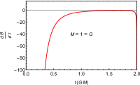
Figure 1: Left: $\frac{d\theta}{d\tau}$ as a function of the Schwarzschild time $t$. Right: negative branch of $\theta$ as a function of $t$. Both $\theta$ and $\frac{d\theta}{d\tau}$ diverge as we approach $t\to 0$. Note that the divergence at the horizon is due to the choice of Schwarzschild coordinate system.

4.2 Effective dynamics and Raychaudhuri equation

The effective behavior of the interior of the Schwarzschild black hole can be deduced from its effective Hamiltonian (constraint). There are various equivalent ways to obtain such an effective Hamiltonian from the classical one [5, 10, 7, 6, 16]. It turns out that the easiest way is by replacing

$$b\to \frac{\sin\left(\mu_{b}b\right)}{\mu_{b}},$$ (18)

$$c\to \frac{\sin\left(\mu_{c}c\right)}{\mu_{c}},$$ (19)

in the classical Hamiltonian.

The free parameters $\mu_{b},\,\mu_{c}$ are the minimum scales associated with the radial and angular directions [5, 7, 10, 29]. If these $\mu$ parameters are taken to be constant, the corresponding approach is called the $\mu_{0}$ scheme. If, however, these parameters depend on the conjugate momenta, the approach is called improved dynamics which itself is divided into various subcategories. In case of the Schwarzschild interior and due to lack of matter content, it is not clear which scheme yields the correct semiclassical limit. Hence, for completeness, in this paper we will study the effective theory in the constant $\mu$ scheme, which here we call the $\mathring{\mu}$ scheme, as well as in two of the most common improved schemes, which we denote by $\bar{\mu}$ and $\bar{\mu}^{\prime}$ schemes.

Replacing (18) and (19) into the classical Hamiltonian (5), one obtains an effective Hamiltonian constraint,

$$H_{\textrm{eff}}^{(N)}=-\frac{N}{2G\gamma^{2}}\left[\left(\frac{\sin^{2}\left(\mu_{b}b\right)}{\mu_{b}^{2}}+\gamma^{2}\right)\frac{p_{b}}{\sqrt{p_{c}}}+2\frac{\sin\left(\mu_{b}b\right)}{\mu_{b}}\frac{\sin\left(\mu_{c}c\right)}{\mu_{c}}\sqrt{p_{c}}\right].$$ (20)

In order to be able to compare the effective results with the classical case, we need to use the same lapse as we did in the classical part. Under (18), this lapse (14) becomes

$$N=\frac{\gamma\mu_{b}\sqrt{p_{c}}}{\sin\left(\mu_{b}b\right)}.$$ (21)

Using this in (20) we obtain

$$H_{\textrm{eff}}=-\frac{1}{2\gamma G}\left[p_{b}\left[\frac{\sin\left(\mu_{b}b\right)}{\mu_{b}}+\gamma^{2}\frac{\mu_{b}}{\sin\left(\mu_{b}b\right)}\right]+2p_{c}\frac{\sin\left(\mu_{c}c\right)}{\mu_{c}}\right].$$ (22)

Note that both (20) and (22) reduce to their classical counterparts (5) and (15) respectively, as is expected.

To obtain the effective Raychadhuri equation, we consider three cases:

1. $\mathring{\mu}$ scheme where $\mu_{b}=\mathring{\mu}_{b}$ and $\mu_{c}=\mathring{\mu}_{c}$ are constants,

2. $\bar{\mu}$ scheme where we set

   $$\mu_{b}=\bar{\mu}_{b}= \sqrt{\frac{\Delta}{p_{b}}},$$ (23)

   $$\mu_{c}=\bar{\mu}_{c}= \sqrt{\frac{\Delta}{p_{c}}},$$ (24)

3. $\bar{\mu}^{\prime}$ scheme where we choose

   $$\mu_{b}=\bar{\mu}_{b}^{\prime}= \sqrt{\frac{\Delta}{p_{c}}},$$ (25)

   $$\mu_{c}=\bar{\mu}_{c}^{\prime}= \frac{\sqrt{p_{c}\Delta}}{p_{b}}.$$ (26)

   After replacing these (separately for each case) into the effective Hamiltonian constraint (22) and finding their corresponding equations of motion [30], one replaces the solutions in the Raychadhuri equation (11) to obtain the form of $\frac{d\theta}{d\tau}$. It turns out that for all the three cases above we obtain

   $$\frac{d\theta}{d\tau}= \frac{1}{\gamma^{2}p_{c}}\frac{\sin^{2}\left(\mu_{b}b\right)}{\mu_{b}^{2}}\left[\cos\left(\mu_{b}b\right)\cos\left(\mu_{c}c\right)-\frac{\cos^{2}\left(\mu_{b}b\right)}{4}-3\cos^{2}\left(\mu_{c}c\right)\right]$$

   $$+\frac{\cos\left(\mu_{b}b\right)}{p_{c}}\left[\frac{\cos\left(\mu_{b}b\right)}{2}-\cos\left(\mu_{c}c\right)-\frac{\gamma^{2}}{4}\cos\left(\mu_{b}b\right)\frac{\mu_{b}^{2}}{\sin^{2}\left(\mu_{b}b\right)}\right],$$ (27)

   where it is understood that $\mu$’s should be substituted for from cases 1–3 suitably for each case.

4.2.1 $\mathring{\mu}$ scheme

Let us first consider this case perturbatively in an analytic manner. Replacing $\mu_{b}=\mathring{\mu}_{b}$ and $\mu_{c}=\mathring{\mu}_{c}$ as constants in (27) and then expanding for small values of $\mu$’s up to the second order we obtain

$$\frac{d\theta}{d\tau}\approx-\frac{1}{2p_{c}}\left(1+\frac{9b^{2}}{2\gamma^{2}}+\frac{\gamma^{2}}{2b^{2}}\right)+\mathring{\mu}_{b}^{2}\frac{1}{2p_{c}}\left(\frac{b^{4}}{\gamma^{2}}+\frac{\gamma^{2}}{3}\right)+\mathring{\mu}_{c}^{2}\frac{c^{2}}{2p_{c}}\left(1+\frac{5b^{2}}{\gamma^{2}}\right).$$ (28)

It is seen that the first term on the right-hand side above is the classical expression (17) which is always negative and leads to the divergence of classical expansion rate at the singularity, i.e., infinite focusing. However, Eq. (28) now involves two additional effective terms proportional to $\mathring{\mu}_{b}^{2}$ and $\mathring{\mu}_{c}^{2}$, both of which are positive. Furthermore, from the solutions to equations of motion [30], one can infer that these two terms take over close to where the classical singularity used to be and stop $\theta$ and $\frac{d\theta}{d\tau}$ from diverging. This can, in fact, be confirmed by looking at the full nonperturbative behavior of $\frac{d\theta}{d\tau}$ plotted in Fig. 2. There, it is seen that the quantum gravity effects counter the attractive nature of classical terms and turn the curve around such that $\frac{d\theta}{d\tau}$ goes to zero for $t\to 0$.

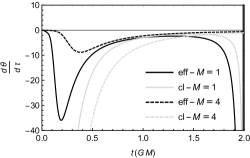
Figure 2: Plot of $\frac{d\theta}{d\tau}$ as a function of the Schwarzschild time $t$, for two different masses in classical vs effective regimes. The figure is plotted using $\gamma=0.5,\,G=1,\,L_{0}=1$, and $\mathring{\mu}_{b}=0.08=\mathring{\mu}_{c}$.

4.2.2 $\bar{\mu}$ scheme

Similar to the $\mathring{\mu}$ scheme we start by analyzing the perturbative expansion of $\frac{d\theta}{d\tau}$ for this case by replacing (23) and (24) in (27) and expanding it for small $\bar{\mu}$’s up to the lowest correction terms which in this case is $\Delta$ (which can be considered as the second order in $\bar{\mu}$ scales). This way we get

$$\frac{d\theta}{d\tau}\approx-\frac{1}{2p_{c}}\left(1+\frac{9b^{2}}{2\gamma^{2}}+\frac{\gamma^{2}}{2b^{2}}\right)+\frac{\Delta}{p_{c}}\left[\frac{1}{6p_{b}}\left(\frac{3b^{4}}{\gamma^{2}}+\gamma^{2}\right)+\frac{c^{2}}{2p_{c}}\left(1+\frac{5b^{2}}{\gamma^{2}}\right)\right].$$ (29)

Once again, the first term on the right-hand side is the classical expression of the Raychaudhuri equation (17), which contributes to infinite focusing at the singularity, but all the correction terms are positive and take over close to the position of the classical singularity. This stops $\frac{d\theta}{d\tau}$ from diverging similar to the $\mathring{\mu}$ scheme.

Figure 3: Left: Raychaudhuri equation in the $\bar{\mu}$ scheme. Right: Raychaudhuri equation vs $p_{c}$. The vertical dot-dashed line at $t\approx 0.43GM$ is the position of the bounce of $p_{c}$ where its minimum $p_{c}^{\textrm{min}}=0.29$ happens in this case. The figure is plotted using $\gamma=0.5,\,M=1,\,G=1,\,L_{0}=1$, and $\Delta=0.1$.

The full nonperturbative form of the modified Raychaudhuri equation in terms of $t$ can also be plotted plotted by substituting the numerical solutions of the equations of motion for the $\bar{\mu}$ in (27). The result is plotted in Fig. 3. We see that, approaching from the horizon to where the classical singularity used to be, an initial bump or bounce in encountered, followed by a more pronounced bounce closer to where the singularity used to be. Once again, the quantum corrections become dominant close to the singularity and turn back the $\frac{d\theta}{d\tau}$ such that at $t\to 0$ no focusing happens at all. Furthermore, from the right plot in Fig. 3, we see that the first bounce in the Raychaudhuri equation happens much earlier than the bounce in $p_{c}$ for this batch of geodesics.

4.2.3 $\bar{\mu}^{\prime}$ scheme

The perturbative analytical form of $\frac{d\theta}{d\tau}$ for this case, up to the first correction term turns out to be

$$\frac{d\theta}{d\tau}\approx-\frac{1}{2p_{c}}\left(1+\frac{9b^{2}}{2\gamma^{2}}+\frac{\gamma^{2}}{2b^{2}}\right)+\frac{\Delta}{6\gamma^{2}}\left[\frac{1}{p_{c}^{2}}\left(3b^{4}+\gamma^{4}\right)+\frac{3c^{2}}{p_{b}^{2}}\left(5b^{2}+\gamma^{2}\right)\right].$$ (30)

Although this perturbative form of the Raychaudhuri equation is a bit different from previous cases, nevertheless it exhibits the property that the quantum corrections are all positive and take over close to where the classical singularity used to be, and hence once again contribute to defocusing of the geodesics. This case is, however, rather different from the previous two cases since the behavior of some of the canonical variables as a function of the Schwarzschild time $t$ deviates significantly from those cases. In particular, both $b$ and $p_{c}$ show a kind of damped oscillatory behavior close to the classical singularity [30], which contributes to a more volatile behavior of the Raychaudhuri equation.

Figure 4: Raychaudhuri equation in the $\bar{\mu}^{\prime}$ scheme. The top left figure shows the behavior over the whole $0\leq t\leq 2GM$ range. Other plots show various close-ups of that plot over smaller ranges of $t$. The figure is plotted using $\gamma=0.5,\,M=1,\,G=1,\,L_{0}=1$, and $\Delta=0.1$.

The full nonperturbative Raychaudhuri equation and its close-ups in this case are plotted in Fig. 4. It is seen that in this scheme, the Raychaudhuri equation exhibits a more oscillatory behavior and has various bumps particularly when we get closer to where the singularity used to be. Very close to the classical singularity, its form resembles those of $b$ and $p_{c}$, behaving like a damped oscillation [30].

Two particular features are worth noting in this scheme. First, as we also saw in previous schemes, quantum corrections kick in close to the singularity and dominate the evolution such that the infinite focusing is remedied, hence signaling the resolution of the singularity. Second, this scheme exhibits a nonvanishing value for $\frac{d\theta}{d\tau}$ at, or very close to, the singularity. In Fig. 4 with the particular choice of numerical values of $\gamma,\,M,\,G,\,L_{0}$ and $\Delta$, the value of $\frac{d\theta}{d\tau}$ for $t\to 0$ is approximately $-5.5$. Hence, although a nonvanishing focusing is not achieved in this case at where the singularity used to be, nevertheless, there exists a relatively small focusing and certainly $\frac{d\theta}{d\tau}$ remains finite.

5 Discussion and outlook

In this work, we probed the structure of the interior of the Schwarzschild black hole, particularly the region close to the classical singularity, using the effective Raychaudhuri equation. The effective terms in this equation result from considering the effective modifications to the Hamiltonian of the interior due to polymer quantization, which is equivalent to loop quantization of this model. We found out that while the classical rate of expansion $\frac{d\theta}{d\tau}$ diverges for $r\to 0$, the effective terms counter such a divergence close to the singularity and make $\frac{d\theta}{d\tau}$ finite at $r\to 0$. We considered three main schemes of polymer quantization and the results hold in all three. This is a strong indication that LQG points to the resolution of the singularity in the effective regime.

It is also worth noting that very similar behavior has been derived recently for several cases of Generalized Uncertainty Principle (GUP) models [31, 32]. In particular, it seems that these cases bare a significant resemblance to $\mathring{\mu}$ and $\bar{\mu}$. This can be taken as a cross-model affirmation that quantum gravity in general does resolve the singularity of the Schwarzschild black hole.

References

- [1] A. Raychaudhuri, Relativistic cosmology. 1., Phys. Rev. 98, 1123 (1955).
- [2] R. Penrose, Gravitational collapse and space-time singularities, Phys. Rev. Lett. 14, 57 (1965).
- [3] S. Hawking and R. Penrose, The Singularities of gravitational collapse and cosmology, Proc. Roy. Soc. Lond. A 314, 529 (1970).
- [4] T. Thiemann, Modern Canonical Quantum General RelativityCambridge Monographs on Mathematical Physics, Cambridge Monographs on Mathematical Physics (Cambridge University Press, 2007).
- [5] A. Ashtekar and M. Bojowald, Quantum geometry and the Schwarzschild singularity, Class. Quant. Grav. 23, 391 (2006).
- [6] Böhmer, Christian G. and Vandersloot, Kevin, Loop Quantum Dynamics of the Schwarzschild Interior, Phys. Rev. D 76, p. 104030 (2007).
- [7] A. Corichi and P. Singh, Loop quantization of the Schwarzschild interior revisited, Class. Quant. Grav. 33, p. 055006 (2016).
- [8] A. Ashtekar, J. Olmedo and P. Singh, Quantum extension of the Kruskal spacetime, Phys. Rev. D 98, p. 126003 (2018).
- [9] M. Bojowald and S. Brahma, Signature change in loop quantum gravity: Two-dimensional midisuperspace models and dilaton gravity, Phys. Rev. D 95, p. 124014 (2017).
- [10] D.-W. Chiou, Phenomenological loop quantum geometry of the Schwarzschild black hole, Phys. Rev. D 78, p. 064040 (2008).
- [11] A. Corichi, A. Karami, S. Rastgoo and T. Vukašinac, Constraint Lie algebra and local physical Hamiltonian for a generic 2D dilatonic model, Class. Quant. Grav. 33, p. 035011 (2016).
- [12] R. Gambini, J. Olmedo and J. Pullin, Spherically symmetric loop quantum gravity: analysis of improved dynamics, Class. Quant. Grav. 37, p. 205012 (2020).
- [13] R. Gambini, J. Pullin and S. Rastgoo, New variables for 1+1 dimensional gravity, Class. Quant. Grav. 27, p. 025002 (2010).
- [14] S. Rastgoo, A local true Hamiltonian for the CGHS model in new variables (4 2013).
- [15] A. Corichi, J. Olmedo and S. Rastgoo, Callan-Giddings-Harvey-Strominger vacuum in loop quantum gravity and singularity resolution, Phys. Rev. D 94, p. 084050 (2016).
- [16] H. A. Morales-Técotl, S. Rastgoo and J. C. Ruelas, Effective dynamics of the Schwarzschild black hole interior with inverse triad corrections (6 2018).
- [17] J. Olmedo, S. Saini and P. Singh, From black holes to white holes: a quantum gravitational, symmetric bounce, Class. Quant. Grav. 34, p. 225011 (2017).
- [18] L. Modesto, Black hole interior from loop quantum gravity, Adv. High Energy Phys. 2008, p. 459290 (2008).
- [19] A. Ashtekar, T. Pawlowski and P. Singh, Quantum nature of the big bang, Phys. Rev. Lett. 96, p. 141301 (2006).
- [20] A. Ashtekar, T. Pawlowski and P. Singh, Quantum Nature of the Big Bang: An Analytical and Numerical Investigation. I., Phys. Rev. D 73, p. 124038 (2006).
- [21] A. Ashtekar, S. Fairhurst and J. L. Willis, Quantum gravity, shadow states, and quantum mechanics, Class. Quant. Grav. 20, 1031 (2003).
- [22] A. Corichi, T. Vukasinac and J. A. Zapata, Polymer Quantum Mechanics and its Continuum Limit, Phys. Rev. D 76, p. 044016 (2007).
- [23] H. A. Morales-Técotl, S. Rastgoo and J. C. Ruelas, Path integral polymer propagator of relativistic and nonrelativistic particles, Phys. Rev. D 95, p. 065026 (2017).
- [24] H. A. Morales-Técotl, D. H. Orozco-Borunda and S. Rastgoo, Polymer quantization and the saddle point approximation of partition functions, Phys. Rev. D 92, p. 104029 (2015).
- [25] E. Flores-González, H. A. Morales-Técotl and J. D. Reyes, Propagators in Polymer Quantum Mechanics, Annals Phys. 336, 394 (2013).
- [26] A. Joe and P. Singh, Kantowski-Sachs spacetime in loop quantum cosmology: bounds on expansion and shear scalars and the viability of quantization prescriptions, Class. Quant. Grav. 32, p. 015009 (2015).
- [27] S. Saini and P. Singh, Geodesic completeness and the lack of strong singularities in effective loop quantum Kantowski–Sachs spacetime, Class. Quant. Grav. 33, p. 245019 (2016).
- [28] C. Collins, Global structure of the Kantowski-Sachs cosmological models, J. Math. Phys. 18, p. 2116 (1977).
- [29] D.-W. Chiou, Phenomenological dynamics of loop quantum cosmology in Kantowski-Sachs spacetime, Phys. Rev. D 78, p. 044019 (2008).
- [30] K. Blanchette, S. Das, S. Hergott and S. Rastgoo, Black hole singularity resolution via the modified Raychaudhuri equation in loop quantum gravity, Phys. Rev. D 103, p. 084038 (2021).
- [31] P. Bosso, O. Obregón, S. Rastgoo and W. Yupanqui, Deformed algebra and the effective dynamics of the interior of black holes, Class. Quant. Grav. 38, p. 145006 (2021).
- [32] K. Blanchette, S. Das and S. Rastgoo, Effective GUP-modified Raychaudhuri equation and black hole singularity: four models, JHEP 09, p. 062 (2021).