Vortical Quantum Memory

Abstract

Quantum memory is a crucial component of a quantum information processor, just like a classical memory is a necessary ingredient of a conventional computer. Moreover, quantum memory of light would serve as a quantum repeater needed for quantum communication networks. Here we propose to realize the quantum memory coupled to magnetic modes of electromagnetic radiation (e.g. those found in cavities and optical fibers) using vortices in Quantum Hall systems. We describe the response to an external magnetic mode as a quench, and find that it sets an oscillation between vortices and antivortices, with the period controlled by the amplitude of the magnetic mode, and the phase locked to the phase of the magnetic mode. We support our proposal by real-time Hamiltonian field theory simulations.

I Introduction

The development of quantum computers and quantum communications requires quantum memory that stores a quantum state for later retrieval. Of particular interest is a quantum memory that can couple directly to electromagnetic radiation. The main challenge in developing a robust quantum memory is overcoming noise and decoherence. This naturally draws attention to systems in which decoherence can be reduced to a minimum. Because of this, here we propose to consider Quantum Hall systems (realized in topological materials with a gapped bulk [1, 2, 3, 4]) – with their topologically protected edge modes [5, 6, 7, 8], they offer a promise of long coherence time and reduced dissipation. Quantum Hall effect [9, 10, 11, 12] continuously finds new applications and new connections emerge, including its relevance for the Langlands program pointed out recently [13, 14, 15, 16, 17].

Quantum Hall systems can be controlled by an external magnetic flux, such as the one created by magnetic modes in cavities and optical fibers. In this paper we will utilize a two-band model of a Quantum Hall system that describes vortices and antivortices that occur in the Brillouin zone of a Quantum Hall material. The ground state, depending on the value of an external magnetic flux, contains antivortices, or no vortices or antivortices at all. However when a rapid change in the external magnetic flux occurs (we will call this a “topological quench”, as it changes the topology of the system), the quantum state becomes a superposition of vortices and antivortices, with a phase determined by the moment of time when the quench took place. As we will show below, the period of quantum oscillations between vortices and antivortices is determined by the amplitude of the external magnetic flux, and varies in a very wide interval. Therefore, both the phase and the amplitude of an electromagnetic wave are recorded in the Quantum Hall state, which thus makes it a quantum memory.

Traditionally, quantum Hall effect (QHE) requires an external magnetic field. The QHE however appears even without an external magnetic field in magnetic topological insulators. A topological insulator is a material that exhibits a metallic state on the surface while the interior is in an insulating state. A magnetic topological insulator can be created through a proximity effect due to the presence of magnetic dopants, or it can be a ferromagnetic material with internal magnetization. The interplay between the metallic state of the surface and ferromagnetism generates the quantum Hall effect even in the absence of a magnetic field [18, 19]. This phenomenon is called the quantum anomalous Hall (QAH) effect, which is distinct from the integer quantum Hall effect, because edge currents can be generated without the application of an external magnetic field.

It is tempting to think of this topological quantum system with periodic oscillations between vortices and antivortices in terms of a “topological time crystal”, but our quantum state is not a ground state of the Quantum Hall system at a given value of an external magnetic flux. Instead, it is an excited state formed by the topological quench, and the time evolution of this quantum state is controlled by the parameters of the quench. The paper is organized as follows. In Section II we describe the two-band model of the Quantum Anomalous Hall systems that we use, discuss the vortices and antivortices that it contains, and outline the topological quench protocol that we use in our real-time Hamiltonian field theory simulation. In Section II.4 we present the results of our real-time simulation, and show that the parameters of topological quench are indeed encoded in the phase and period of quantum vortex-antivortex oscillation that we observe. Finally, in Section III we discuss the results and present an outlook for future studies.

II Topological Quench in Quantum Hall System

II.1 The two-band model

Here we consider the quantum anomalous Hall effect, which occurs when the external magnetic field is zero but the spins are polarized. This model is described by the following simple two-band Hamiltonian [20]

$$\begin{aligned} H&=\sum_{i}R_{i}(m,k_{x},k_{y})\sigma_{i},\\ R_{x}&=\sin k_{x},R_{y}=\sin k_{y},R_{z}=m-\cos k_{x}-\cos k_{y}.\end{aligned}$$ (1)

The physical interpretation of this model in terms of the relevant degrees of freedom depends on it material realization – for example, the two bands can represent either different spin states of electrons with a spin-orbit interaction, or orbital degrees of freedom with band hybridization.

This model has the high symmetry points $k_{i}=0,\pi$, i.e. momentum points at the edges and center that represent all combinations of $k_{i}=0,\pi$ for each direction of $k_{i}$: $(0,0),(\pi,0),(0,\pi),(\pi,\pi)$. As plotted in Fig.1, there is a band crossing point at $m=-2$ if $k_{x}=k_{y}=\pi$, at which the energy gap decreases as $m$ approaches -2. These are the points around which the vortices of Berry curvature are localized. As we will explain in detail below, we construct the topological invariant of these vortices by assigning the $\mathbb{Z}_{2}$-index to the vortex based on its rotation direction : clockwise (-1) or anticlockwise (+1).

The lower band has the eigenvalue and the eigenstate

$$E(k) =-\sqrt{R_{x}(k)^{2}+R_{y}(k)^{2}+R_{z}(k)^{2}}$$ (2)

$$\ket{\Psi^{A}(k)} =\frac{1}{N_{A}}\begin{pmatrix}R_{z}(k)-|R(k)|\\ R_{x}(k)-iR_{y}(k)\end{pmatrix},$$ (3)

where $N_{A}$ is the normalization factor. This wave function becomes ill-defined if $R_{z}\geq 0$ and $R_{x}(k)=R_{y}(k)=0$. In our case, this happens for example at $k_{x}=k_{y}=\pi$, $m>-2$.

There is another way to express the same state by shifting the phase

$$\ket{\Psi^{B}(k)}=\frac{\frac{R_{z}+|R|}{R_{x}+iR_{y}}}{\bigg{|}\frac{R_{z}+|R|}{R_{x}+iR_{y}}\bigg{|}}\ket{\Psi^{A}(k)}=\frac{1}{N_{B}}\begin{pmatrix}-R_{x}(k)+iR_{y}(k)\\ R_{z}(k)+|R(k)|\end{pmatrix},$$ (4)

which is well-defined at $R_{z}>0$ and $R_{x}(k)=R_{y}(k)=0$. This wave function becomes ill-defined if $R_{z}\leq 0$ and $R_{x}(k)=R_{y}(k)=0$. In our case, this happens for example at $k_{x}=k_{y}=0$ of $m<2$.

II.2 Vortices and anti-vortices

Because the wave function is ill-defined at some points in the Brillouin zone, we need to remove these points by cutting the Brillouin zone into two and using two different representations of the wave function. These representations are connected by a gauge transformation

$$\ket{\Psi^{B}}=e^{i\phi(k)}\ket{\Psi^{A}}.$$ (5)

The Berry connection

$$\mathcal{A}^{l}(k)=-i\bra{\psi^{l}(k)}d\psi^{l}(k)\rangle,$$ (6)

is transformed as

$$\mathcal{A}^{B}=\mathcal{A}^{A}+\nabla_{k}\phi(k).$$ (7)

Let us discuss the structure of the ground state for different values of magnetic flux.

• For $m>2$, $R_{z}(k)$ is always positive for all the four high symmetry points. So we can use $\Psi^{B}(k)$ for the entire Brillouin zone. Therefore the first Chern number

  $$C=\frac{1}{2\pi}\int_{T_{\text{BZ}}}d^{2}kd\mathcal{A}^{B}$$ (8)

  is zero, $C=0$, and no vortices and antivortices exist.

• For $0<m<2$, $R_{z}(k)$ is negative at $(0,0)$ and positive at the other three points $(\pi,\pi),(0,\pi),(\pi,0)$. So we can choose $\Psi^{A}$ around a small disk of $(0,0)$ and $\Psi^{B}$ outside of it. By taking the disk sufficiently small, we find $\phi(k)=-\theta$ and $C=\frac{1}{2\pi}\int_{0}^{2\pi}d\theta\partial_{\theta}\phi=-1$, which corresponds to an antivortex.

• For $-2<m<0$, $R_{z}(k)$ is positive at $(\pi,\pi)$ and negative at the other three points $(\pi,\pi),(0,\pi),(\pi,0)$. So we can choose $\Psi^{B}$ around a small disk of $(\pi,\pi)$ and $\Psi^{A}$ outside of it. By repeating the same argument, we again find $C=-1$.

• For $m<-2$, $R_{z}(k)$ is negative for all the four special points. So we can use $\Psi^{A}(k)$ for the entire Brillouin zone. Therefore $C=0$.

• We cannot define the Chern number for $m=0,\pm 2$, where the gap closes.

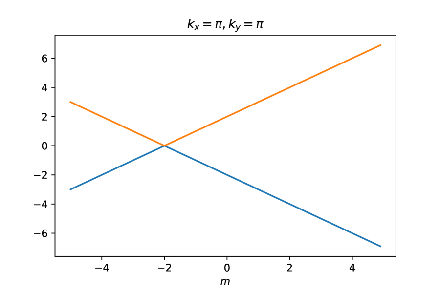
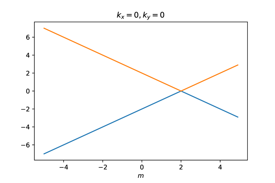
Figure 1: Energy eigenvalues at $k_{x}=k_{y}=\pi$ and $0$.

The Hall conductance associated with the $l$-th band is explained by the Kubo formula [21, 22, 23, 24]

$$\begin{aligned} \sigma^{l}_{xy}&=-\frac{e^{2}}{h}\frac{1}{2\pi}\int_{T_{\text{BZ}}}d^{2}kd\mathcal{A}^{l}=-\frac{e^{2}}{h}\ C\end{aligned}$$ (9)

where $\psi^{l}(k)$ is the $l$-th Bloch function. We consider a quench process of $\psi^{l}$

$$\ket{\psi^{l}(t,k)}=e^{-itH^{\prime}}\ket{\psi^{l}(k)},$$ (10)

where $H^{\prime}=H(m^{\prime})$, and then we find the time-dependent Berry connection,

$$\mathcal{A}^{l}(t,k)=-i\bra{\psi^{l}(t,k)}d\psi^{l}(t,k)\rangle.$$ (11)

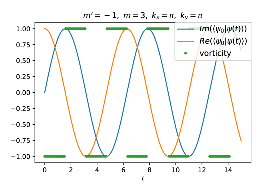
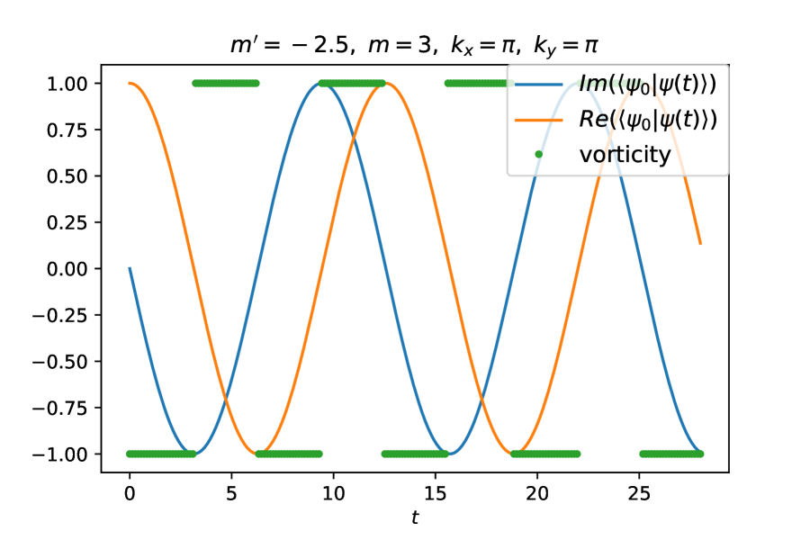
Figure 2: Mass dependence of vorticity change near $k_{x}=k_{y}=\pi$. [Left] $m^{\prime}=1.0$, [Middle] $m^{\prime}=-1.0$, [Right] $m^{\prime}=-2.5$.

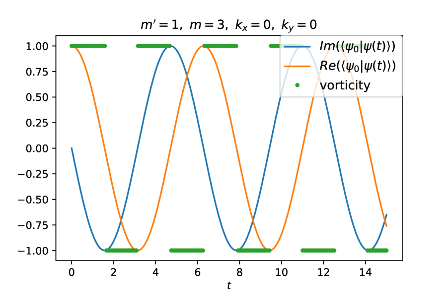
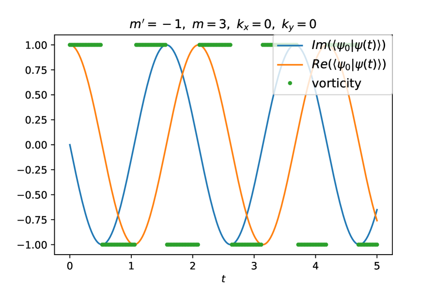
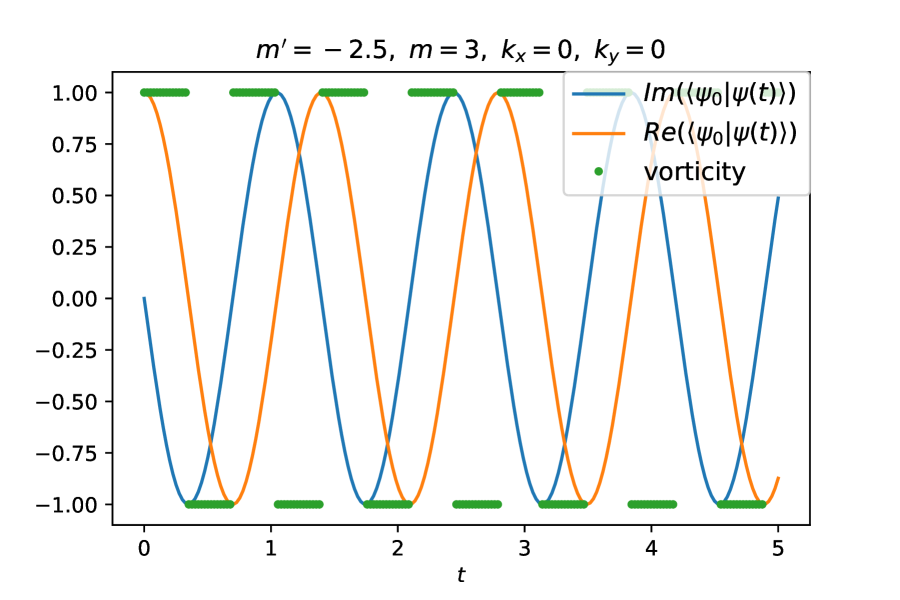
Figure 3: Mass dependence of vorticity change near $k_{x}=k_{y}=0$. [Left] $m^{\prime}=1.0$, [Middle] $m^{\prime}=-1.0$, [Right] $m^{\prime}=-2.5$.

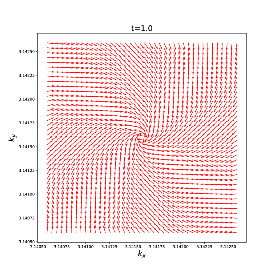
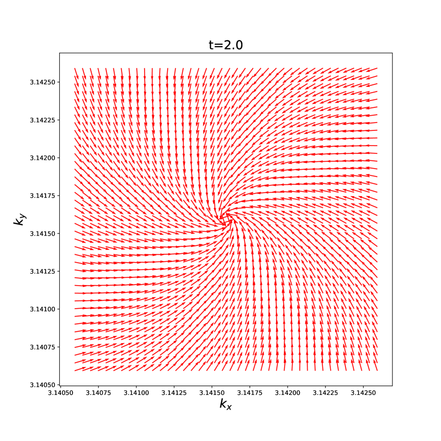
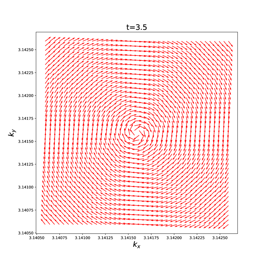
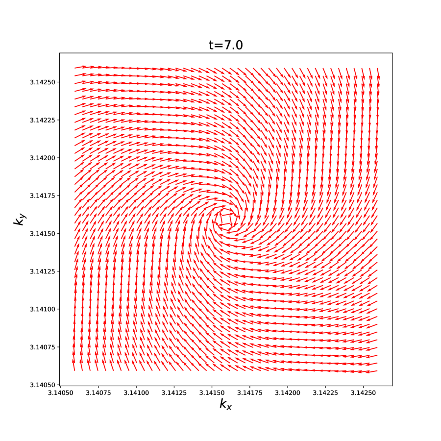
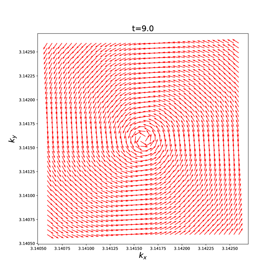
Figure 4: Time evolution of the vortex after quench at $k_{x}=k_{y}=\pi$.

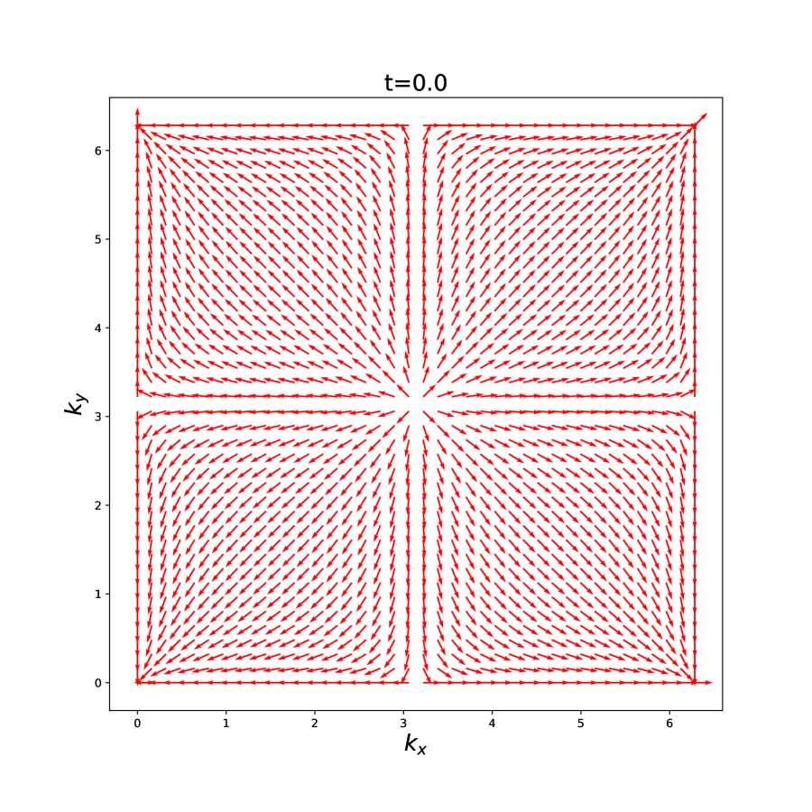
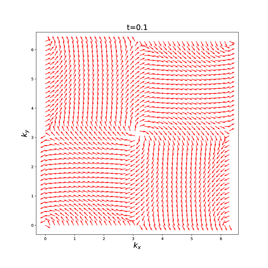
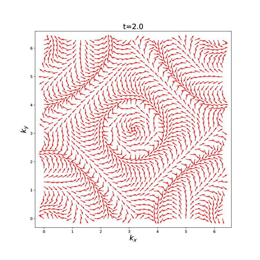
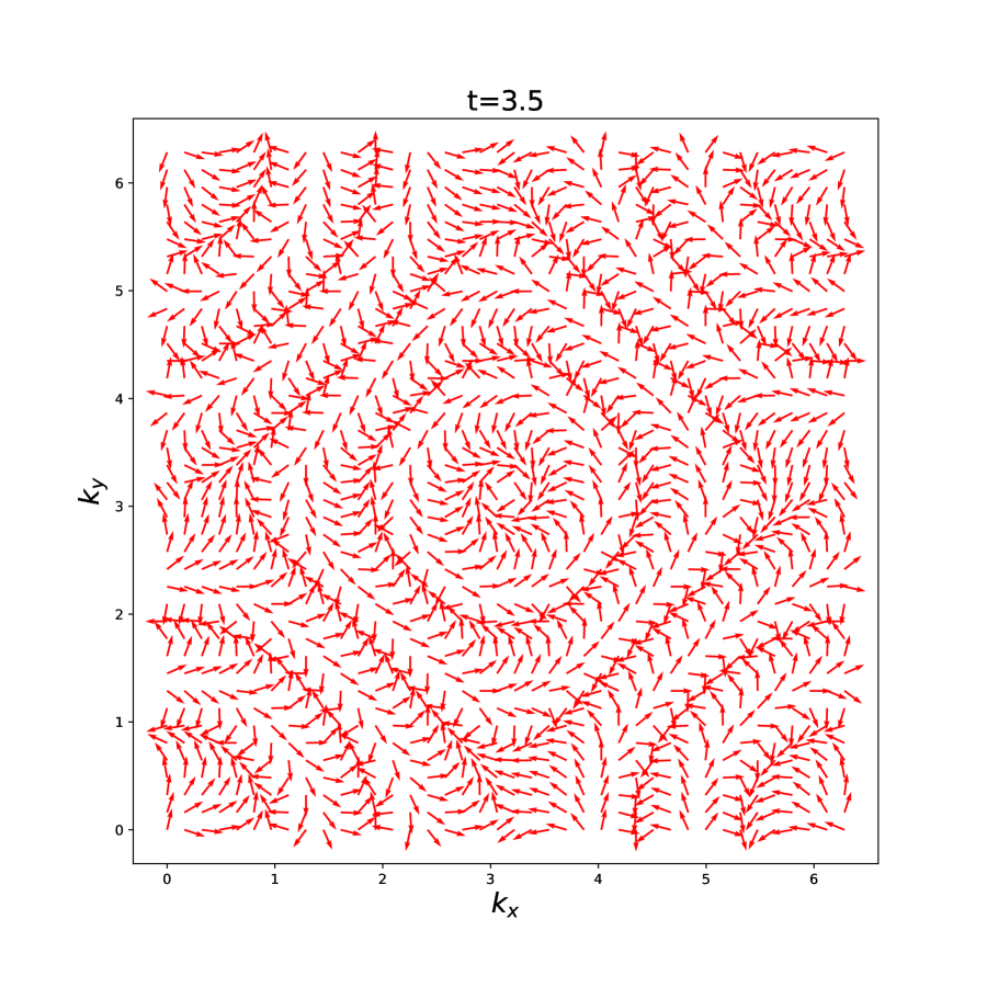
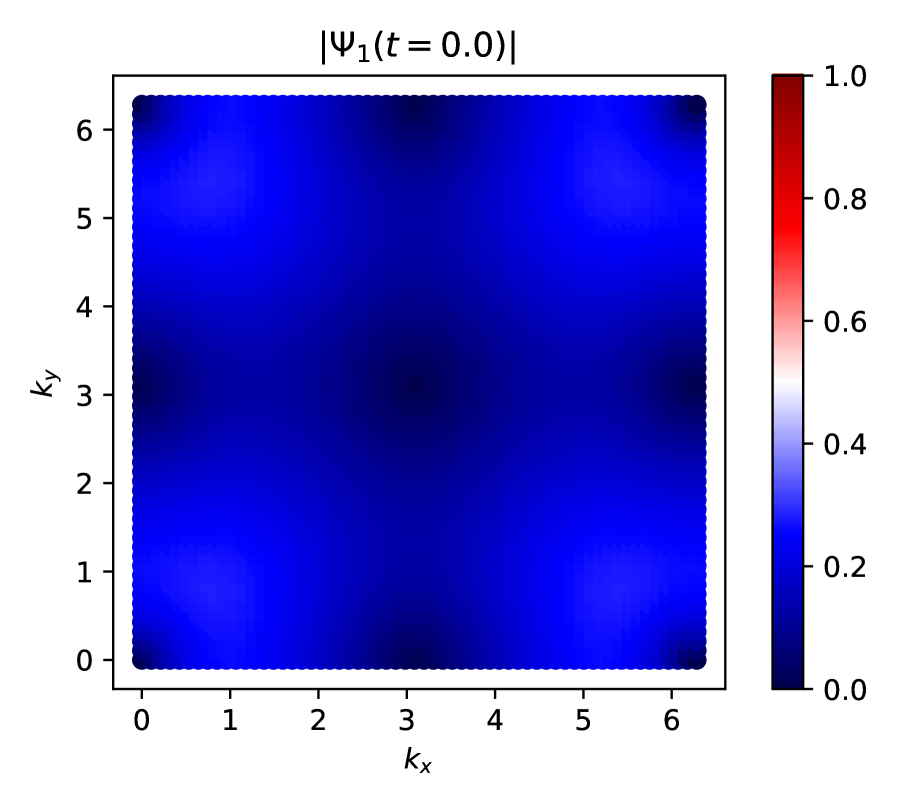
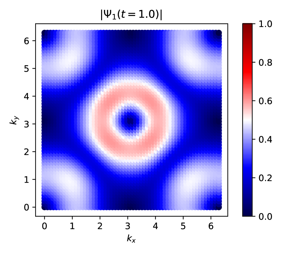
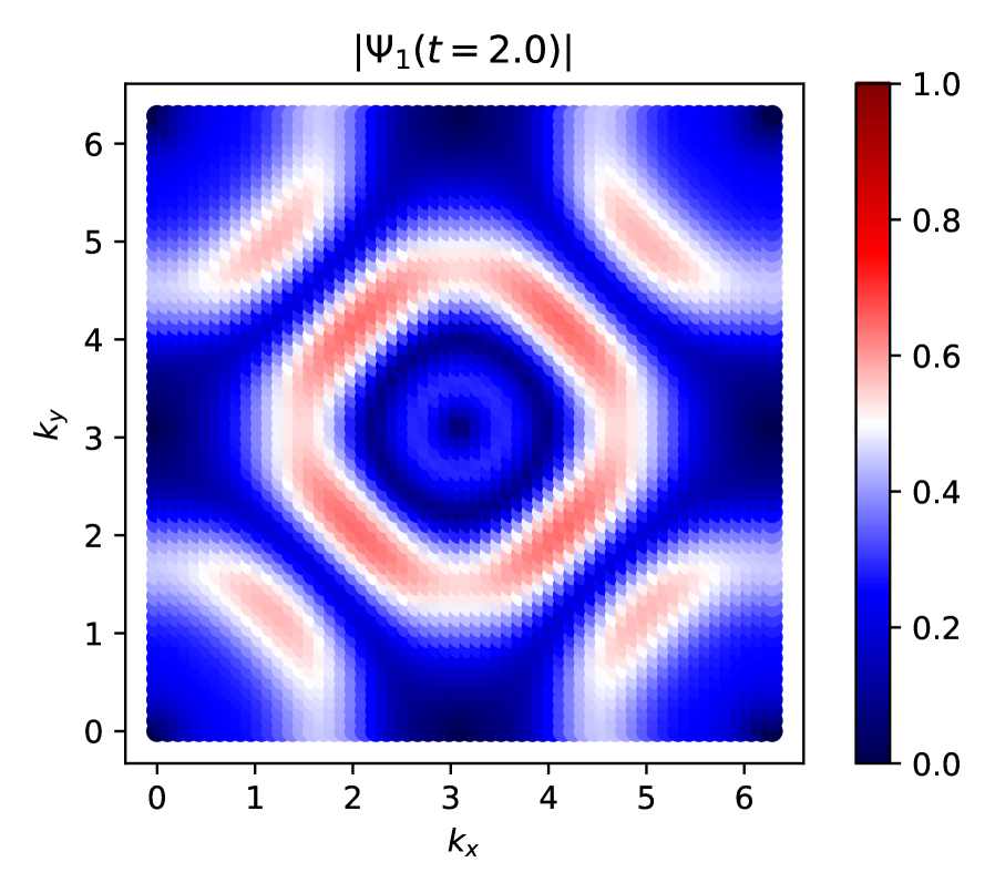
Figure 5: Time evolution of the vortex after quench. [Bottom] Time evolution of the density corresponding to the first component of the state after quench.

II.3 Vortices and topology

In general the Berry connection possesses several vortices in the magnetic Brillouin zone. Here we are going to discuss the definition of the Chern number in this more general case.

The two Bloch states $\ket{\Psi^{A}},\ket{\Psi^{B}}$ defined in different gauges are related by

$$\ket{\Psi^{B}(t,k)}=e^{i\xi_{BA}(t,k)}\ket{\Psi^{A}(t,k)}.$$ (12)

For an arbitrary Bloch state $\ket{\Psi}$, we choose a complex number $\xi_{A}$ such that the second component of $\Psi^{A}$ is strictly positive:

$$\begin{aligned} \ket{\Psi^{A}}&=e^{-i\text{Arg}\,\xi_{A}}\ket{\Psi},\quad(\Psi^{A})_{2}>0.\end{aligned}$$ (13)

This is possible everywhere except for zeros of $\xi_{A}$. We will assume that these zeros are isolated, and define $S_{i},(i=1,\cdots,N)$ as small disks around each of them. Around those zeros, we define $\Psi^{B}$ by

$$\begin{aligned} \ket{\Psi^{B}}&=e^{-i\text{Arg}\,\xi_{B}}\ket{\Psi},\quad(\Psi^{B})_{1}>0,\end{aligned}$$ (14)

again choosing the phase of $\xi_{B}$ such that the first component of $\Psi^{B}$ is positive. Then the gauge transformation is given by

$$\xi_{BA}=\text{Im log}\frac{\xi_{A}}{\xi_{B}}.$$ (15)

Therefore, due to the Stokes theorem, given $S=\bigcup_{i=1}^{N}S_{i}$, the Chern number associated with the Berry connection can be written as

$$\begin{aligned} C(t)&=\frac{1}{2\pi}\int_{S}d^{2}kd\mathcal{A}^{B}+\frac{1}{2\pi}\int_{T_{\text{BZ}}\setminus S}d^{2}kd\mathcal{A}^{B},\\ &=\frac{1}{2\pi}\sum_{i=1}^{N}\oint_{\partial S_{i}}dk\cdot(\mathcal{A}^{B}-\mathcal{A}^{A})\\ &=\sum_{i=1}^{N}\frac{1}{2\pi}\oint_{\partial S_{i}}dk\cdot\nabla\xi_{BA}(t,k).\end{aligned}$$ (16)

Consequently the total Chern number is related to the total vorticity of Bloch state.

II.4 Topological quench protocol

In our quench protocol, we put the system in the ground state at an initial value of $m$, and then at time $t=0$ abruptly change $m$ to a new value of $m^{\prime}$. We then measure the Loschmidt amplitude, which is a measure of fidelity between two quantum states in a quench process:

$$L_{m\to m^{\prime}}(t) =\bra{\psi_{n,m}}e^{-itH_{m^{\prime}}}\ket{\psi_{n,m}},$$ (17)

where $\psi_{n,m}$ is the $n$-th eigenstate of the Hamiltonian $H_{m}$ with mass $m$. The Loschmidt amplitude has been used for detecting dynamical quantum phase transitions in  [25, 26].

For $m>2$ (when there are no vortices in the ground state), we use $\ket{\Psi_{\text{in}}}=\ket{\Psi^{B}}$ for the initial state and consider time evolution of vortices after quench, when $|m^{\prime}|<2$. For $|m^{\prime}|<2$ we use the ground state $\ket{\Psi^{B}}$ or $\ket{\Psi^{A}}$ around a circle at $(\pi,\pi)$. The subsequent time evolution for $|m^{\prime}|<2$ described by $e^{-itH_{m^{\prime}}}\ket{\Psi_{\text{in}}}$ corresponds to the gauge transformation.

The local vortex evolution is shown in Fig. 4, and the time evolution of the vector field over the entire Brillouin zone is shown in Fig. 5. As it is clear from Fig. 4, the direction of the vortex at $k_{x}=k_{y}=\pi$ changes periodically. We can assign the $\mathbb{Z}_{2}$-index to the vortex based on its rotation direction : clockwise (-1) or anticlockwise (+1). Fig. 5 exhibits the vortex at $(k_{x},k_{y})=(\pi,\pi)$ and Fig. 5 [Bottom] shows the time evolution of the ground state density (lower band). Fig. 2 and 3 show the variation of Loschmidt amplitude and vorticity at $k_{x}=k_{y}=\pi$ and 0, respectively.

Our numerical calculations reveal that the time at which the sign of the real or imaginary part of the Loschmidt amplitude changes coincides with the time at which the vorticity changes, and that plateaus with constant vorticity appear periodically in time. Oscillations between vortices and antivortices have been reported before [27], with the period $2\pi/\Delta E$, where $\Delta E$ is the energy difference between the two bands. Fig. 6 clearly shows that this law is perfectly valid in our case (see also Fig. 1). The vortices at $k_{x}=k_{y}=\pi$ and $0$ have different periods, indicating that quantum memories with different periods are created in the Brillouin zone. The change in vorticity in the vicinity of $m=-2$ is shown in Fig. 7, where its period is very long for $k_{x}=k_{y}=\pi$ (see also Fig. 8), while the period for $k_{x}=k_{y}=0$ is short. These results indicate the scaling of the period with the inverse band gap.

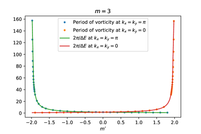
Figure 6: $m^{\prime}$-dependence of the period of vorticity oscillations at $k_{x}=k_{y}=\pi$. The initial mass is set to $m=3$.

III Discussion and outlook

Quantum memory records a quantum state for later retrieval. Various quantum memories have been theoretically proposed and are being actively explored experimentally [28, 29, 30, 31, 32, 33]. Our proposal provides a simple topological quantum memory that can be realized with a single qubit operator. The system of oscillating vortices and antivortices records information about the amplitude of an electromagnetic wave (encoded through the magnetic flux parameter $m$ of the Hamiltonian) through the period of oscillations, and about its phase. Therefore, both the phase and the amplitude of an electromagnetic wave are recorded in the Quantum Hall state, which thus makes it a quantum memory. Moreover, the period of oscillations varies in a very wide interval depending on the external magnetic flux.

Readout of the quantum state recorded in this “vortical quantum memory” can be realized optically since the reflection and transmission of electromagnetic waves will be affected by the presence of oscillating vortices and the resulting from them oscillating Quantum Hall conductivity. In fact, the two-band model used in this study has already been implemented in many methods, such as photonic crystals [34] microwave resonators [35], superconducting qubit [36], phononic metamaterials [37], and its topological properties have been investigated. Clearly, the theory of this electromagnetic readout should be developed quantitatively. We leave this for a future investigation.

It will also be interesting to investigate the possibility of realizing quantum memory in other traditional class [38, 39, 40] and new class of topological models, e.g. those described in [41, 42, 43, 44, 45].

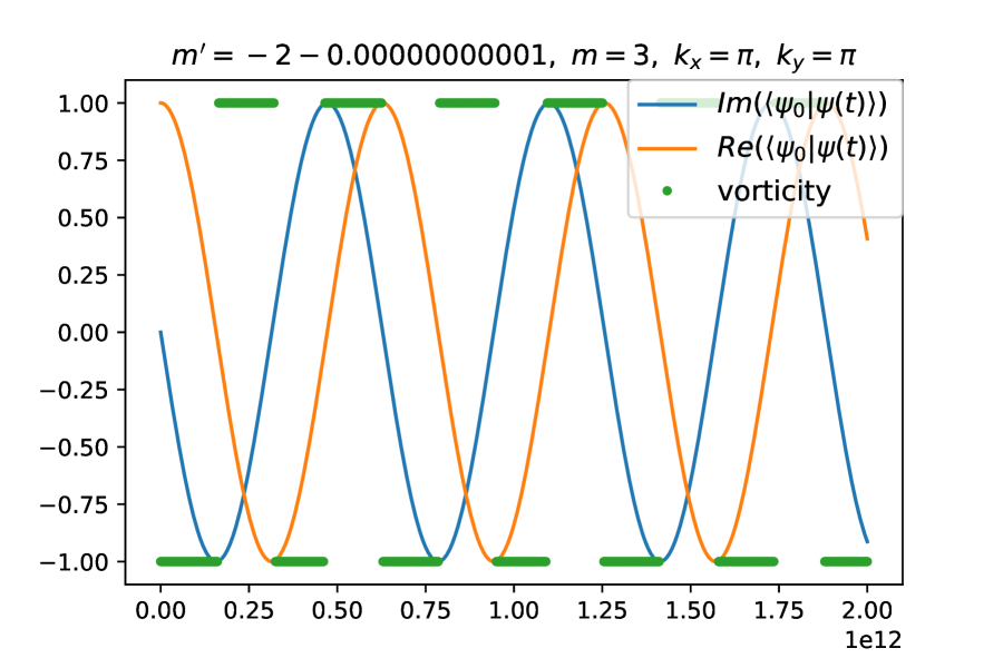
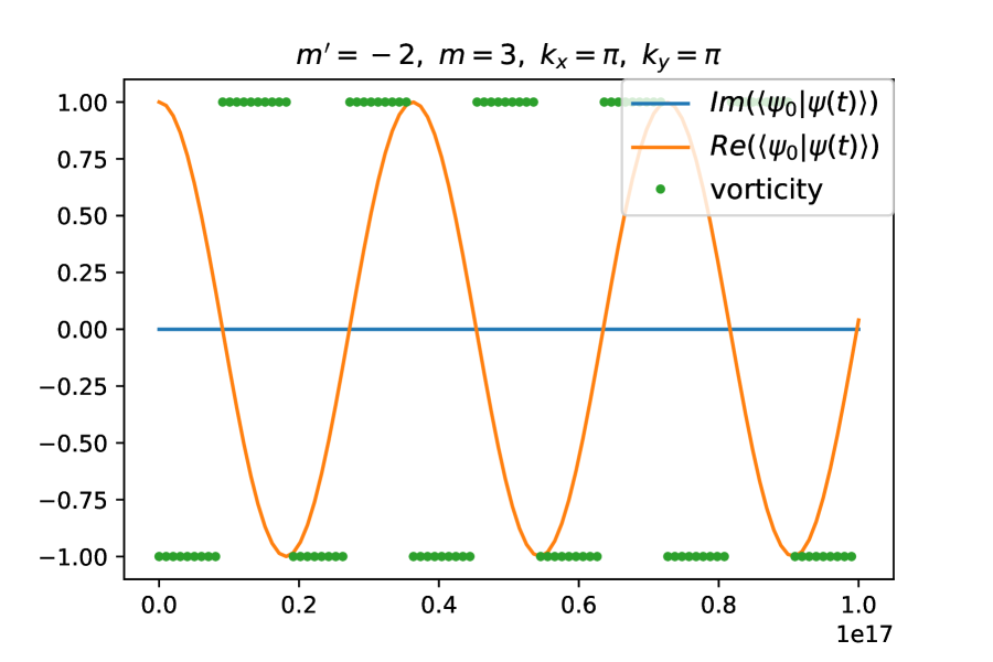
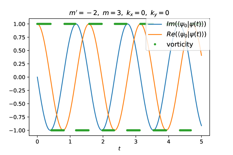
Figure 7: Vorticity at $m=-2,k_{x}=k_{y}=\pi$ [Left and Middle] and at $m=-2,k_{x}=k_{y}=0$.

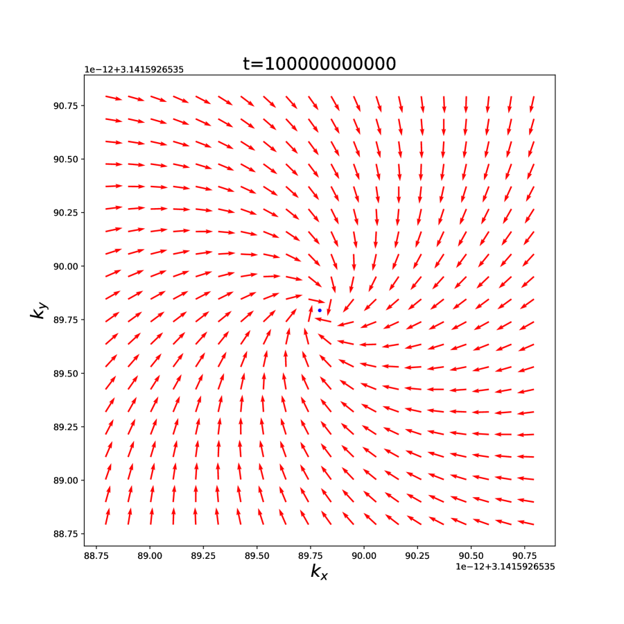
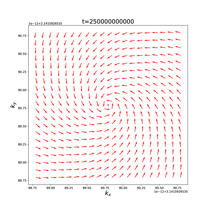
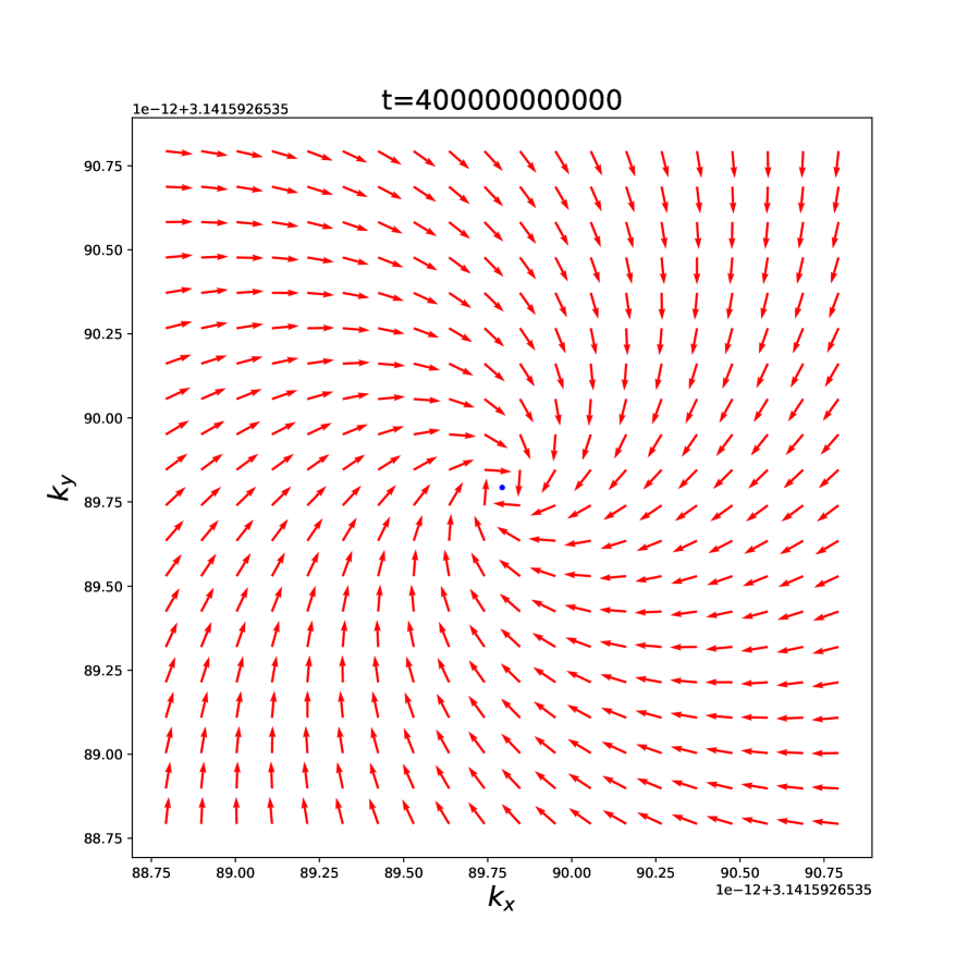
Figure 8: Vortex at $m=-2-0.00000000001$ at $k_{x}=k_{y}=\pi$

References

- [1] X.-L. Qi, T. L. Hughes, and S.-C. Zhang, “Topological field theory of time-reversal invariant insulators,” Physical Review B 78 no. 19, (2008) 195424.
- [2] A. P. Schnyder, S. Ryu, A. Furusaki, and A. W. W. Ludwig, “Classification of topological insulators and superconductors in three spatial dimensions,” Physical Review B 78 no. 19, (Nov., 2008) 195125, arXiv:0803.2786 [cond-mat.mes-hall].
- [3] R.-J. Slager, A. Mesaros, V. Juričić, and J. Zaanen, “The space group classification of topological band-insulators,” Nature Physics 9 no. 2, (2013) 98–102.
- [4] H. C. Po, A. Vishwanath, and H. Watanabe, “Complete theory of symmetry-based indicators of band topology,” Nature Communications 8 (June, 2017) 50, arXiv:1703.00911 [cond-mat.str-el].
- [5] Y. Hatsugai, “Chern number and edge states in the integer quantum hall effect,” Phys. Rev. Lett. 71 (Nov, 1993) 3697–3700. https://link.aps.org/doi/10.1103/PhysRevLett.71.3697.
- [6] Y. Hatsugai, “Edge states in the integer quantum hall effect and the riemann surface of the bloch function,” Physical Review B 48 no. 16, (1993) 11851.
- [7] K. Kawabata, K. Shiozaki, and M. Ueda, “Anomalous helical edge states in a non-hermitian chern insulator,” Physical Review B 98 no. 16, (2018) 165148.
- [8] R. Süsstrunk and S. D. Huber, “Observation of phononic helical edge states in a mechanical topological insulator,” Science 349 no. 6243, (2015) 47–50.
- [9] T. Ando, Y. Matsumoto, and Y. Uemura, “Theory of hall effect in a two-dimensional electron system,” Journal of the Physical Society of Japan 39 no. 2, (1975) 279–288, https://doi.org/10.1143/JPSJ.39.279. https://doi.org/10.1143/JPSJ.39.279.
- [10] R. B. Laughlin, “Quantized hall conductivity in two dimensions,” Phys. Rev. B 23 (May, 1981) 5632–5633. https://link.aps.org/doi/10.1103/PhysRevB.23.5632.
- [11] D J Thouless, “Localisation and the two-dimensional hall effect,” Journal of Physics C: Solid State Physics 14 no. 23, (1981) 3475. http://stacks.iop.org/0022-3719/14/i=23/a=022.
- [12] K. v. Klitzing, G. Dorda, and M. Pepper, “New method for high-accuracy determination of the fine-structure constant based on quantized hall resistance,” Phys. Rev. Lett. 45 (Aug, 1980) 494–497. https://link.aps.org/doi/10.1103/PhysRevLett.45.494.
- [13] K. Ikeda, “Quantum hall effect and langlands program,” Annals of Physics 397 (2018) 136 – 150.
- [14] K. Ikeda, “Hofstadter’s butterfly and langlands duality,” Journal of Mathematical Physics 59 no. 6, (2018) 061704, https://doi.org/10.1063/1.4998635. https://doi.org/10.1063/1.4998635.
- [15] K. Ikeda, “Topological Aspects of Matters and Langlands Program,” arXiv e-prints (Dec., 2018) arXiv:1812.11879, arXiv:1812.11879 [cond-mat.mes-hall].
- [16] Y. Matsuki and K. Ikeda, “Comments on the fractal energy spectrum of honeycomb lattice with defects,” Journal of Physics Communications 3 no. 5, (May, 2019) 055003. https://doi.org/10.1088/2399-6528/ab18de.
- [17] Y. Matsuki, K. Ikeda, and M. Koshino, “Fractal defect states in the hofstadter butterfly,” Phys. Rev. B 104 (Jul, 2021) 035305. https://link.aps.org/doi/10.1103/PhysRevB.104.035305.
- [18] C.-Z. Chang, J. Zhang, X. Feng, J. Shen, Z. Zhang, M. Guo, K. Li, Y. Ou, P. Wei, L.-L. Wang, Z.-Q. Ji, Y. Feng, S. Ji, X. Chen, J. Jia, X. Dai, Z. Fang, S.-C. Zhang, K. He, Y. Wang, L. Lu, X.-C. Ma, and Q.-K. Xue, “Experimental Observation of the Quantum Anomalous Hall Effect in a Magnetic Topological Insulator,” Science 340 no. 6129, (Apr., 2013) 167–170, arXiv:1605.08829 [cond-mat.mes-hall].
- [19] C.-X. Liu, S.-C. Zhang, and X.-L. Qi, “The quantum anomalous hall effect: Theory and experiment,” Annual Review of Condensed Matter Physics 7 (2016) 301–321.
- [20] X.-L. Qi, Y.-S. Wu, and S.-C. Zhang, “Topological quantization of the spin hall effect in two-dimensional paramagnetic semiconductors,” Phys. Rev. B 74 (Aug, 2006) 085308. https://link.aps.org/doi/10.1103/PhysRevB.74.085308.
- [21] R. Kubo, “Statistical-mechanical theory of irreversible processes. i. general theory and simple applications to magnetic and conduction problems,” Journal of the Physical Society of Japan 12 no. 6, (1957) 570–586, https://doi.org/10.1143/JPSJ.12.570. https://doi.org/10.1143/JPSJ.12.570.
- [22] A. Widom, “Thermodynamic derivation of the Hall effect current,” Physics Letters A 90 (Aug., 1982) 474–474.
- [23] P. Streda, “Theory of quantised hall conductivity in two dimensions,” Journal of Physics C: Solid State Physics 15 no. 22, (1982) L717. http://stacks.iop.org/0022-3719/15/i=22/a=005.
- [24] D. J. Thouless, M. Kohmoto, M. P. Nightingale, and M. den Nijs, “Quantized hall conductance in a two-dimensional periodic potential,” Phys. Rev. Lett. 49 (Aug, 1982) 405–408. https://link.aps.org/doi/10.1103/PhysRevLett.49.405.
- [25] X.-Y. Hou, Q.-C. Gao, H. Guo, Y. He, T. Liu, and C.-C. Chien, “Ubiquity of zeros of the Loschmidt amplitude for mixed states in different physical processes and its implication,” Phys. Rev. B 102 no. 10, (Sept., 2020) 104305, arXiv:2006.12445 [quant-ph].
- [26] T. V. Zache, N. Mueller, J. T. Schneider, F. Jendrzejewski, J. Berges, and P. Hauke, “Dynamical topological transitions in the massive Schwinger model with a -term,” arXiv e-prints (Aug., 2018) arXiv:1808.07885, arXiv:1808.07885 [quant-ph].
- [27] G. Watanabe and C. J. Pethick, “Reversal of the circulation of a vortex by quantum tunneling in trapped Bose systems,” Physical Review A 76 no. 2, (Aug., 2007) 021605, arXiv:cond-mat/0701270 [cond-mat.mes-hall].
- [28] A. I. Lvovsky, B. C. Sanders, and W. Tittel, “Optical quantum memory,” Nature photonics 3 no. 12, (2009) 706–714.
- [29] M. P. Hedges, J. J. Longdell, Y. Li, and M. J. Sellars, “Efficient quantum memory for light,” Nature 465 no. 7301, (2010) 1052–1056.
- [30] Y. Wang, J. Li, S. Zhang, K. Su, Y. Zhou, K. Liao, S. Du, H. Yan, and S.-L. Zhu, “Efficient quantum memory for single-photon polarization qubits,” Nature Photonics 13 no. 5, (2019) 346–351.
- [31] B. Julsgaard, J. Sherson, J. I. Cirac, J. Fiurášek, and E. S. Polzik, “Experimental demonstration of quantum memory for light,” Nature 432 no. 7016, (2004) 482–486.
- [32] H. P. Specht, C. Nölleke, A. Reiserer, M. Uphoff, E. Figueroa, S. Ritter, and G. Rempe, “A single-atom quantum memory,” Nature 473 no. 7346, (2011) 190–193.
- [33] E. Dennis, A. Kitaev, A. Landahl, and J. Preskill, “Topological quantum memory,” Journal of Mathematical Physics 43 no. 9, (2002) 4452–4505.
- [34] J. Noh, W. A. Benalcazar, S. Huang, M. J. Collins, K. Chen, T. L. Hughes, and M. C. Rechtsman, “Topological protection of photonic mid-gap cavity modes,” arXiv e-prints (Nov., 2016) arXiv:1611.02373, arXiv:1611.02373 [cond-mat.mes-hall].
- [35] C. W. Peterson, W. A. Benalcazar, T. L. Hughes, and G. Bahl, “A quantized microwave quadrupole insulator with topologically protected corner states,” Nature 555 no. 7696, (2018) 346–350.
- [36] J. Niu, T. Yan, Y. Zhou, Z. Tao, X. Li, W. Liu, L. Zhang, H. Jia, S. Liu, Z. Yan, Y. Chen, and D. Yu, “Simulation of higher-order topological phases and related topological phase transitions in a superconducting qubit,” Science Bulletin 66 no. 12, (2021) 1168–1175. https://www.sciencedirect.com/science/article/pii/S2095927321001766.
- [37] M. Serra-Garcia, V. Peri, R. Süsstrunk, O. R. Bilal, T. Larsen, L. G. Villanueva, and S. D. Huber, “Observation of a phononic quadrupole topological insulator,” Nature 555 no. 7696, (2018) 342–345.
- [38] F. D. M. Haldane, “Model for a quantum hall effect without landau levels: Condensed-matter realization of the ”parity anomaly”,” Phys. Rev. Lett. 61 (Oct, 1988) 2015–2018. https://link.aps.org/doi/10.1103/PhysRevLett.61.2015.
- [39] C. L. Kane and E. J. Mele, “ topological order and the quantum spin hall effect,” Phys. Rev. Lett. 95 (Sep, 2005) 146802. https://link.aps.org/doi/10.1103/PhysRevLett.95.146802.
- [40] F. Pollmann, E. Berg, A. M. Turner, and M. Oshikawa, “Symmetry protection of topological phases in one-dimensional quantum spin systems,” Phys. Rev. B 85 (Feb, 2012) 075125. https://link.aps.org/doi/10.1103/PhysRevB.85.075125.
- [41] S. Yu, X. Piao, and N. Park, “Topological Hyperbolic Lattices,” Physical Review Letters 125 no. 5, (July, 2020) 053901, arXiv:2003.07002 [physics.optics].
- [42] A. Jahn, M. Gluza, F. Pastawski, and J. Eisert, “Majorana dimers and holographic quantum error-correcting codes,” Physical Review Research 1 no. 3, (Nov., 2019) 033079, arXiv:1905.03268 [hep-th].
- [43] J. Maciejko and S. Rayan, “Hyperbolic band theory,” Science Advances 7 no. 36, (2021) eabe9170, https://www.science.org/doi/pdf/10.1126/sciadv.abe9170. https://www.science.org/doi/abs/10.1126/sciadv.abe9170.
- [44] K. Ikeda, S. Aoki, and Y. Matsuki, “Hyperbolic band theory under magnetic field and dirac cones on a higher genus surface,” Journal of Physics: Condensed Matter 33 no. 48, (Sep, 2021) 485602. https://doi.org/10.1088/1361-648x/ac24c4.
- [45] S. Aoki, K. Ikeda, and Y. Matsuki, “Algebra of Hyperbolic Band Theory under Magnetic Field,” arXiv e-prints (July, 2021) arXiv:2107.10586, arXiv:2107.10586 [math-ph].