Truncated Rank-Based Tests for Two-Part Models with Excessive Zeros and Applications to Microbiome Data

Wanjie Wanglabel=e1]wanjie.wang@nus.edu.sg [    Eric Chenlabel=e2] [    Hongzhe Lilabel=e2 [    mark]hongzhe@upenn.edu National University of Singapore, University of Pennsylvania,

Supplementary Materials

Wanjie Wanglabel=e1]wanjie.wang@nus.edu.sg [    Eric Chenlabel=e2] [    Hongzhe Lilabel=e2 [    mark]hongzhe@upenn.edu National University of Singapore, University of Pennsylvania,
Abstract

High-throughput sequencing technology allows us to test the compositional difference of bacteria in different populations. One important feature of human microbiome data is that it often includes a large number of zeros. Such data can be treated as being generated from a two-part model that includes a zero point-mass. Motivated by analysis of such non-negative data with excessive zeros, we introduce several truncated rank-based two-group and multi-group tests, including a truncated rank-based Wilcoxon rank-sum test for two-group comparison and two truncated Kruskal-Wallis tests for multi-group comparisons. We show both analytically through asymptotic relative efficiency analysis and by simulations that the proposed tests have higher power than the standard rank-based tests in typical microbiome data settings, especially when the proportion of zeros in the data is high. The tests can also be applied to repeated measurements of compositional data via simple within-subject permutations. In a simple before-and-after treatment experiment, the within-subject permutation is similar to the paired rank test. However, the proposed tests handle the excessive zeros, which leads to a better power. We apply the tests to compare the microbiome compositions of healthy children and pediatric Crohn’s disease patients and to assess the treatment effects on microbiome compositions. We identify several bacterial genera that are missed by the standard rank-based tests.

keywords:
Asymptotic relative efficiency; Differential abundance analysis; Two-part model; Truncation;
\arxiv

math.PR/0000000 \startlocaldefs \endlocaldefs

, and

t3This research was supported by NIH grants GM123056 and GM129781. Hongzhe Li is the corresponding author.

1 Introduction

The human microbiome includes all microorganisms in various human body sites such as gut, skin and mouth. Gut microbiome has been shown to be associated with many human diseases, including obesity, diabetes and inflammatory bowel disease (Turnbaugh et al., 2006; Qin et al., 2012; Manichanh et al., 2012). Two high-throughput sequencing based approaches, including 16S ribosomal RNA (rRNA) sequencing and shotgun metagenomic sequencing, are commonly used in microbiome studies (Turnbaugh et al., 2007; Qin et al., 2010). Bioinformatics methods are available for quantifying the microbial relative abundances based on such sequencing data, which typically involve aligning the reads to some known database or marker genes (Huson et al., 2007; Segata et al., 2012). Since the DNA yielding materials are different across different samples, the resulting numbers of sequencing reads vary greatly from sample to sample. In order to make the microbial abundance comparable across samples, the abundance in read counts is usually normalized to the relative abundance of the bacteria observed, which results in high dimensional compositional data. Some of the most widely used metagenomic processing software such as MEGAN (Huson et al., 2007) and MetaPhlAn (Segata et al., 2012) only outputs the relative abundances of the bacterial taxa.

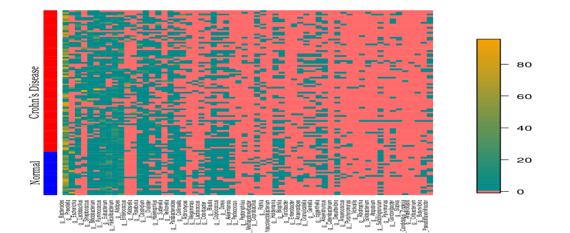
In microbiome studies, one is often interested in identifying the bacterial taxa such as genera or species that show different distributions between two or more conditions. One important feature of microbiome compositional data is that the data include large clumps of zeros that represent the absence of the bacterial taxa in the samples, especially for those relatively rare taxa. Zero observations can also result from under-sampling of the sequencing reads for rare taxa. As an example, Figure 1 shows the heatmap of zeros and the relative abundances for 26 healthy and normal samples and samples from 85 Crohn’s disease children for each of the 60 bacterial genera. These data were collected at the University of Pennsylvania (Lewis et al., 2015). We are interested in identifying the bacterial genera that have different distributions between healthy and Crohn’s disease patients. We observed over 62.5% of the observations are zero. In addition, the compositional data are often skewed, which makes parametric modeling of such data difficult and tests based on parametric distributional assumptions problematic. We present detailed analysis of this data set in Section 6.

Non-parametric tests, such as the Wilcoxon rank-sum test and Kruskal-Wallis test, can be applied to such data and are commonly used in analysis of microbiome data. However, such rank-based tests tend to have low power because of the large number of ties from zero observations (Lachenbruch, 1976, 2001; Hallstrom, 2010). A two-part test combining the square of a test statistic for comparison of the proportion of zeros and the square of an appropriate normal test such as the Wilcoxon rank-sum to compare the non-zero scores was proposed and evaluated by Lachenbruch (2001). This two-part test was recently applied to analysis of microbiome data (Wagner, Robertson and Harris, 2011). However, the theory developed for Lachenbruch’s 2 degree of freedoms $\chi^{2}$ test assumes that binomial test statistic and the test statistics for the continuous part to be independent, which only holds under the assumptions of independent errors of the binomial and continuous part of the distribution (Lachenbruch, 2002). However, such an assumption may not hold for the microbiome relative abundance data generated by sequencing since both can depend on the sequencing depth.

Refer to caption
Figure 1: Heatmap of zeros and the relative abundances of 60 bacterial genera for 26 healthy children and 85 patients with pediatric Crohn’s disease, showing over 62.5% of the observations being zero (Lewis et al., 2015).

To account for excessive zeros in non-negative distributions, Hallstrom (2010) introduced a truncated Wilcoxon rank-sum test, where the Wilcoxon rank-sum test is performed after removing an equal and maximal number of zeros from each sample. He showed that this test recovers much of the power loss from the standard application of the Wilcoxon test. Compared with a directional modification of the two-part test proposed by Lachenbruch (Lachenbruch, 1976, 2001), the truncated Wilcoxon test has similar power when the non-zero relative abundances are independent of the proportion of zeros. In addition, the truncated Wilcoxon test is relatively unaffected when the error terms of the two distributions are dependent. Hallstrom (2010) however only considered the two-sample test under the setting of equal sample sizes.

In this paper, we assume that the data are generated from two-part models with point-mass at zero as one of the components. However, we do not make any distributional assumption on the continuous non-zero part. We develop several rank-based tests for general two-group comparison with possible unequal sample sizes, and for the multiple-group comparisons with equal or unequal sample sizes. Particularly, we extend the truncated Wilcoxon rank-sum test of Hallstrom (2010) to data with unequal sample sizes, and develop a modified Kruskal-Wallis test to account for clumps of zeros for multiple-group comparisons with equal sample sizes and unequal sample sizes, respectively. These new tests are based on the idea of data truncation and asymptotic calculations and can effectively deal with the clumps of zeros in the data. The asymptotic null distributions of the tests are given. The key difficulty of deriving such truncated rank-based tests is to calculate the variance of the test statistic under the null, which does not have a closed-form expression. We instead use asymptotic analysis to obtain approximations of the variance estimates.

In order to demonstrate the advantages of the proposed truncated rank-based tests, we also derive the asymptotic relative efficiency of the proposed tests compared to commonly used Wilcoxon rank-sum test and Kruskal-Wallis test when the data are generated from two-part models (Lachenbruch, 2001). We observe in our simulations large gains in efficiency, especially when the proportions of zeros in the data are high. These tests are rank-based, easy to calculate and provide new tools for identifying the bacterial taxa with different distributions among different groups in human microbiome studies. We apply and compare the proposed tests by analyzing a microbiome study conducted at the University of Pennsylvania (Lewis et al., 2015), including comparing the gut microbiome difference between healthy and pediatric Crohn’s disease patients and assessing the effects of treatment over time.

2 A truncated Wilcoxon rank-sum test for data with excessive zeros

2.1 A truncated Wilcoxon rank-sum test

Consider the two-sample setting where we have $N_{1}$ non-negative independent observations from population 1, $\mathbf{X}=(x(1),\cdots,x(N_{1}))$, and $N_{2}$ independent observations from population 2, $\mathbf{Y}=(y(1),\cdots,y(N_{2}))$, where $x(i)$ (or $y(i)$) represents the relative abundance of a bacterium in the $i$th sample of group 1 (or 2). For most of the bacteria, the data $\mathbf{X}$ and $\mathbf{Y}$ include many zeros, which represent absence of the bacterium in these samples or below detection limits. We are interested in testing whether these observations $\mathbf{X}$ and $\mathbf{Y}$ are from the same distribution, i.e., the hypothesis testing problem that

$$H_{0}:\,\,\mathbf{x}\sim F,\,\mathbf{y}\sim F\qquad vs\qquad H_{1}:\,\,\mathbf{x}\sim F,\,\mathbf{y}\sim G,F\neq G,$$

where $F$ and $G$ are both probability density functions with a proportion of zeros. We consider the two-part model of Lachenbruch (1976), which assumes that the data are generated from the following distributions,

$$x(i)\sim(1-\theta_{1})\delta_{0}+\theta_{1}f,\quad y(j)\sim(1-\theta_{2})\delta_{0}+\theta_{2}g,\quad i=1,\cdots,N_{1},j=1,\cdots,N_{2},$$ (1)

where $\theta_{1}$ (or $\theta_{2}$) is the probability of being non-zero in population $1$ (or $2$), $\delta_{0}$ is point mass at 0, and $f$ (or $g$) is the distribution for nonzero element in the population 1 (or 2).

Because of the excessive zeros, the standard non-parametric Wilcoxon rank-sum test statistic is less effective. A truncated Wilcoxon rank-sum test statistic has been proposed by Hallstrom (2010) for the case $N_{1}=N_{2}=N$. We first extend his test to the general setting where $N_{1}\neq N_{2}$, and examine the asymptotic relative efficiency compared to the standard Wilcoxon test statistic.

Given $\mathbf{X}$ and $\mathbf{Y}$, denote $n_{1}$ (or $n_{2}$) as the number of non-zero observations in $\mathbf{X}$ (or $\mathbf{Y}$) and let $p_{1}$ (or $p_{2}$) be the proportion of non-zero observations in $\mathbf{X}$ (or $\mathbf{Y}$), where $p_{1}=n_{1}/N_{1}$ (or $p_{2}=n_{2}/N_{2}$). Let $p=\max\{p_{1},p_{2}\}$. Let $\lfloor a\rfloor$ denote the largest integer that is smaller than $a$. We rank the combined observations $\mathbf{X}\cup\mathbf{Y}$ from the largest to the smallest so that zeros have the highest ranks, where the tied measurements are given the average rank. For $\mathbf{X}$ (or $\mathbf{Y}$), we keep only $\lfloor{pN_{1}}\rfloor$ (or $\lfloor{pN_{2}}\rfloor$) observations with the smallest ranks, which implies that the observations removed are all zeros. The truncated samples are denoted as $\tilde{\mathbf{X}}$ and $\tilde{\mathbf{Y}}$, respectively. Let $R$ denote the sum of the ranks of all observations in $\mathbf{X}$. The Wilcoxon test statistic can be written as

$$T_{W}=\frac{S^{2}}{\mathrm{Var}[S]},\quad\mbox{where }S=R-\frac{N_{1}+N_{2}+1}{2}N_{1},$$ (2)

and $\mathrm{Var}[S]$ is the variance of $S$ under the null hypothesis.

The same procedure can be applied to the truncated data $\tilde{\mathbf{X}}$ and $\tilde{\mathbf{Y}}$. Rank the combined observations $\tilde{\mathbf{X}}\cup\tilde{\mathbf{Y}}$, from the largest to the smallest, and let $r$ denote the sum of ranks of all observations in $\tilde{\mathbf{X}}$. We define the counterpart of $S$ as

$$s=r-\frac{\lfloor p(N_{1}+N_{2})\rfloor+1}{2}\lfloor pN_{1}\rfloor-\frac{1}{4}\frac{p_{1}+p_{2}}{2}\left(1-\frac{p_{1}+p_{2}}{2}\right)(N_{2}-N_{1}),$$

and define the truncated Wilcoxon test statistic as

$$T_{tW}=\frac{s^{2}}{\mathrm{Var}[s]}.$$

The statistic $s$ is very similar to $S$, except an extra term

$$\frac{1}{4}\frac{p_{1}+p_{2}}{2}\left(1-\frac{p_{1}+p_{2}}{2}\right)(N_{2}-N_{1}),$$

which is caused by the difference between the variances due to different sample sizes. This term disappears when $N_{1}=N_{2}$. Under the alternative hypothesis, this term is a small order term compared to the other part of $s$. Under the null hypothesis, this extra term is used to eliminate the effect of different sample sizes, leading to an expectation close to 0.

To calculate $\mathrm{Var}[s]$ and to derive the asymptotic distribution of $s$, we show that under the null that both $\mathbf{x}$ and $\mathbf{y}$ follow the same distribution with a point mass at 0, when $N_{1}\rightarrow\infty$, $N_{2}\rightarrow\infty$, we have

$${\mathrm{E}}[S]=0,\qquad{\mathrm{E}}[s]=O(\max\{N_{1},N_{2}\}),$$

where the remainder $O(\max\{N_{1},N_{2}\})$ is caused by the difference between $\lfloor pN_{1}\rfloor$ (or $\lfloor pN_{1}\rfloor$) and $pN_{1}$ (or $pN_{2}$). In addition, we have

$\displaystyle\mathrm{Var}[S]$ $\displaystyle=$ $\displaystyle\frac{N_{1}^{2}N_{2}^{2}}{4}{\mathrm{E}}\{(p_{2}-p_{1})^{2}\}+\frac{N_{1}N_{2}}{12}{\mathrm{E}}(N_{1}p_{1}^{2}p_{2}+N_{2}p_{1}p_{2}^{2}+p_{1}p_{2}),$
$\displaystyle\mathrm{Var}[s]$ $\displaystyle=$ $\displaystyle\frac{N_{1}^{2}N_{2}^{2}}{4}\mathrm{Var}\{(p_{2}-p_{1})p\}+\frac{N_{1}N_{2}}{12}{\mathrm{E}}(N_{1}p_{1}^{2}p_{2}+N_{2}p_{1}p_{2}^{2}+p_{1}p_{2}),$

(see Supplemental Materials). With these the results, under the null hypothesis, when $N_{1}\rightarrow\infty$, $N_{2}\rightarrow\infty$, and $c\leq N_{1}/N_{2}\leq C$ for some constants $c$ and $C$, we have

$\displaystyle\mathrm{Var}[S]$ $\displaystyle=$ $\displaystyle N_{1}N_{2}(N_{1}+N_{2})\theta(1-\theta+\theta^{2}/3)/4+O(N^{2.5}),$
$\displaystyle\mathrm{Var}[s]$ $\displaystyle=$ $\displaystyle N_{1}N_{2}(N_{1}+N_{2})\theta^{3}(1-\theta+1/3)/4+O(N^{2.5}),$

where $\theta$ is the expected value of the proportion of non-zero observations in the data. Hence, $\sqrt{\mathrm{Var}[s]}=O(\sqrt{N_{1}N_{2}\max\{N_{1},N_{2}\}})$, and ${\mathrm{E}}[s]=O(\max\{N_{1},N_{2}\})$ is relatively small when $N_{1}$ and $N_{2}$ are large. Asymptotically, $s/\sqrt{\mathrm{Var}(s)}$ follows a standard normal distribution, and the truncated Wilcoxon test statistic $T_{tW}=s^{2}/\mathrm{Var}[s]$ has a $\chi^{2}_{1}$ null distribution.

The asymptotic analysis above provides a way of approximating ${\mathrm{Var}}(s)$ using the main term of ${\mathrm{Var}}(s)$, which leads to the final test statistic

$$T_{tW}=\frac{s^{2}}{N_{1}N_{2}(N_{1}+N_{2})(\frac{p_{1}+p_{2}}{2})^{3}(4/3-\frac{p_{1}+p_{2}}{2})/4}.$$

This is used in our simulation and real data analysis.

2.2 Pitman’s asymptotic relative efficiency of $T_{W}$ and $T_{tW}$ for two-sample test

To compare the test statistics $T_{W}$ and $T_{tW}$, we evaluate the asymptotic property of the relative efficiency. Since we reject the null hypothesis when the statistic is large, the Pitman’s relative efficiency is defined as

$$RE(T_{tW},T_{W})=\frac{\mathrm{E}_{1}[T_{tW}]}{\mathrm{E}_{1}[T_{W}]}=\frac{\mathrm{E}_{1}[s^{2}]/\mathrm{Var}[s]}{\mathrm{E}_{1}[S^{2}]/\mathrm{Var}[S]}.$$

Here, ${\mathrm{E}}_{1}$ denotes the expectation of the statistic under the alternative hypothesis. A value larger than one implies power gain using the truncated Wilcoxon test statistic compared to the standard Wilcoxon statistic.

For the two-part model (1), we need some terms to quantify the difference between the two distributions. Let $\theta=(\theta_{1}+\theta_{2})/2$, $\theta_{m}=\max\{\theta_{1},\theta_{2}\}$, and $\triangle\theta=\theta_{2}-\theta_{1}$. Define $\Delta_{f,g}=P(\mathbf{x}<\mathbf{y})+P(\mathbf{x}=\mathbf{y})/2-1/2$, where $\mathbf{x}\sim f$ and $\mathbf{y}\sim g$. The term $\Delta_{f,g}$ is used to measure the effect size of the non-zero part. The following theorem provides an explicit expression for the asymptotic relative efficiency (are).

Theorem 1.

Under model (1) and that $N_{1}\rightarrow\infty$, $N_{2}\rightarrow\infty$, and $c\leq N_{1}/N_{2}\leq C$ holds for some constants $c$ and $C$, then the are can be derived as

$$\displaystyle\textsc{are}(T_{tW},T_{W})=\frac{1}{\theta^{2}}\frac{1-\theta+\theta^{2}/3}{1-\theta+1/3}\biggl{(}\frac{\theta_{1}\theta_{2}\Delta_{f,g}+\triangle\theta\theta_{m}/2}{\theta_{1}\theta_{2}\Delta_{f,g}+\triangle\theta/2}\biggr{)}^{2}+O(N^{-1/2}).$$

Especially, we have that $\mathrm{E}(s|n_{1},n_{2})=n_{1}n_{2}\Delta_{f,g}.$

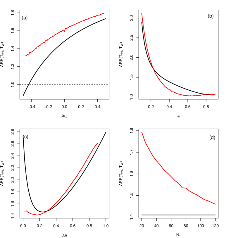
To illustrate the gain in efficiency of using the truncated Wilcoxon test, we present the $\textsc{are}(W_{m},W)$ for the following four different parameter settings to assess the effect of $\Delta_{f,g}$, $\theta$, $\triangle\theta$, and $N_{1}/N_{2}$:

  • (a)

    Effect of $\Delta_{f,g}$: $N_{1}=40$, and $N_{2}=50$ and $\theta_{1}=0.3$, $\theta_{2}=0.8$. Let $\Delta_{f,g}{\color[rgb]{0,0,0}=-1/2+0.01k}$, where $k=0,1,2,\cdots,100$.

  • (b)

    Effect of $\theta$: $N_{1}=40$, $N_{2}=50$, and $\Delta_{f,g}=0.1$. Let $\theta=0.1+0.01k$, where $k=0,1,2,\cdots,80$. With a given $\theta$, take $\theta_{1}=\theta-0.1$ and $\theta_{2}=\theta+0.1$.

  • (c)

    Effect of $\triangle\theta$: $N_{1}=40$, $N_{2}=50$ and $\Delta_{f,g}=0.1$. Let $\triangle\theta=0.02k$, where $k=0,1,2,\cdots,50$. With a given $\triangle\theta$, take $\theta_{1}=0.5-\triangle\theta/2$ and $\theta_{2}=0.5+\triangle\theta/2$.

  • (d)

    Effect of sample size: $\theta_{1}=0.3$, $\theta_{2}=0.8$, $\Delta_{f,g}=0.1$, and $N_{2}=50$. Choose $N_{1}\in\{20,25,30,\cdots,115,120\}$.

Figure 2 shows the are for these four different settings. We observe that ares are larger than one for almost all the parameter settings, indicating that the truncated Wilcoxon statistic has greater power than the standard Wilcoxon statistic. In settings (a) and (b), $\textsc{are}(T_{tW},T_{W})$ increases when $\Delta_{f,g}$ increases or the proportion of zeros increases. Hence, when the nonzero part are away from each other, the truncated test statistic gains more power compared to the standard Wilcoxon statistics. In setting (c), the $\textsc{are}(T_{tW},T_{W})$ function is not monotone due to the cancellation of difference between non-zero part and the non-zero proportions. In setting (d), obviously $\textsc{are}(T_{tW},T_{W})$ does not depend on the value of $N_{1}$ or $N_{2}$, which can be seen in the formula. In Figure 2 (a), when $\Delta_{f,g}$ has a large negative value ($<-0.44$), $\textsc{are}(T_{tW},T_{W})$ is smaller than 1. This is the case when $\Delta_{f,g}$ and $\triangle\theta$ show opposite effects and cancel with each other, leading to a loss of efficiency from the truncation of zeros. However, in real microbiome studies, this scenario is very unlikely to occur since this would imply that individuals who do not carry a particular bacterium have a similar risk as the individuals who have a very high abundance of this same bacterium.

We have further verified the theoretical are using simulations and present the results in Section 1 of the Supplemental Materials. We observe that the simulated are is close to the theoretical are, in terms of both values and the trends as we change the parameters.

Refer to caption
Figure 2: Asymptotic relative efficiency $\textsc{are}(T_{tW},T_{W})$ comparing the truncated Wilcoxon rank test and the standard Wilcoxon rank test as a function of (a) $\Delta_{f,g}$, (b) $\theta$, (c) $\triangle\theta$, and (d) $N_{1}$. For each plot, the horizontal dashed line represents $\textsc{are}(T_{tW},T_{W})=1$.

3 A truncated Kruskal-Wallis test for $K$-group comparison with equal sample sizes

3.1 A truncated Kruskal-Wallis test

Consider the setting where we have data from $K$ groups $\mathbf{X}_{1},\mathbf{X}_{2},\cdots,\mathbf{X}_{K}$, all containing non-negative independent observations from population $1,2,\cdots,K$, respectively. Each group $\mathbf{X}_{i}=(x_{i}(1),\cdots,x_{i}(N_{i}))$ contains $N_{i}$ $i.i.d$ observations. We assume that the samples from the $K$ groups are generated from the following two-part model,

$$x_{i}(j)\sim(1-\theta_{i})\delta_{0}+\theta_{i}f_{i},\quad i=1,\cdots,K.$$ (3)

The hypothesis of interest is

$$H_{0}:\theta_{1}=\cdots=\theta_{K}=\theta,\quad f_{1}=\cdots=f_{K}=f\quad vs\quad H_{1}:\mbox{not all $\theta_{i}$s and $f_{i}$s are equal}.$$

The Kruskal-Wallis test is a standard nonparametric test for $K$-group comparison based on the ranks. We propose to develop a similar rank-based test that accounts for excessive zeros in the two-part model. We first consider the case when the samples sizes from all $K$ groups are the same, i.e., $N_{1}=N_{2}=\cdots=N_{K}=N$. Let $r_{i}(j)$ be the rank of the $j$th observation in the $i$th group among all $KN$ observations. The Kruskal-Wallis statistic can be written as

$$T_{KW}=\frac{12}{KN^{2}(KN+1)}\sum_{i=1}^{K}S_{i}^{2},$$

where $S_{i}=\sum_{j=1}^{N}r_{i}(j)-(KN+1)N/2$. To derive the distribution of $T_{KW}$ under the null hypothesis, we rewrite $T_{KW}$ in terms of $Y_{i}$, where $Y_{i}=\sum_{j=1}^{i}S_{j}-iS_{i+1}$, $1\leq i\leq K-1$,

$$T_{KW}=\frac{12}{KN^{2}(KN+1)}\sum_{i=1}^{K-1}\frac{Y_{i}^{2}}{i(i+1)}=\sum_{i=1}^{K-1}\frac{Y_{i}^{2}}{\mathrm{Var}[Y_{i}]}.$$

With this transformation, $Y_{i}$s are asymptotically independent with each other, and under the null hypothesis, the test statistic $T_{KW}$ is the summation of $K-1$ chi-square random variables with degree of freedom of 1, and therefore is asymptotically distributed as a $\chi^{2}_{K-1}$ distribution.

In order to account for excessive zeros in the data sets, we propose to modify the $T_{KW}$ statistic using the idea of truncation. Let $n_{i}$ denote the number of nonzero observations in group $i$, so the proportion of nonzero entries is $p_{i}=n_{i}/N$. Let $p=\max_{1\leq i\leq K}p_{i}$. For each group $i$, keep the $pN$ observations with smallest ranks (or largest values), so that all the removed entries are zeros. Let $n=pN=\max_{1\leq i\leq K}p_{i}N=\max_{1\leq i\leq K}n_{i}$, then the truncated data set has $Kn$ observations in total. Rank all $Kn$ observations from smallest to largest, and then let $r_{i}$ denote the rank-sum of the observations in group $i$. Define

$$s_{i}=r_{i}-n(Kn+1)/2,\qquad U_{i}=\sum_{j=1}^{i}s_{j}-is_{i+1},\quad 1\leq i\leq K-1,$$

where $s_{K}=-\sum_{i=1}^{K-1}s_{i}$. The following Lemma show that $U_{i}$’s are independent.

Lemma 1.

Under the model that all $x_{i}(j)$ are independently and identically distributed,

$$\mathrm{E}[U_{i}]=0,\qquad\mathrm{Cov}[U_{i_{1}},U_{i_{2}}]=0.$$

This leads to our definition of the truncated Kruskal-Wallis test statistic as

$$T_{tKW}=\sum_{i=1}^{K-1}\frac{U_{i}^{2}}{\mathrm{Var}[U_{i}]},$$

which has a $\chi^{2}$ distribution with degree of freedoms $K-1$ under the null hypothesis. When $K=2$, this statistic becomes the truncated Wilcoxon rank-sum statistic given $N_{1}=N_{2}$. The following Lemma 2 provides an approximation of the variance of $Y_{i}$ and $U_{i}$ under null hypothesis and alternative hypothesis.

Lemma 2.

Consider the two-part model (3). Under the null hypothesis and suppose that $N\rightarrow\infty$, we have

$$\mathrm{Var}[Y_{i}]=\frac{i(i+1)K^{2}N^{3}\theta}{4}\left\{\frac{\theta^{2}}{3}+(1-\theta)\right\}+O(N^{5/2}),\quad 1\leq i\leq K-1;$$
$$\mathrm{Var}[U_{i}]=\frac{i(i+1)K^{2}N^{3}\theta^{3}}{4}\biggl{\{}\frac{1}{3}+(1-\theta)\biggr{\}}+O(N^{5/2}),\quad 1\leq i\leq K-1.$$

Under the alternative hypothesis, we have the upper bound of the variances,

$${\mathrm{Var}}_{1}[Y_{i}]\leq K^{3}N^{3},\quad{\mathrm{Var}}_{1}[U_{i}]\leq K^{3}N^{3},\qquad 1\leq i\leq K.$$

Based on this lemma, the unknown variance ${\mathrm{Var}}[U_{i}]$ can be approximated by

$$\frac{i(i+1)K^{2}N^{3}(\sum_{k=1}^{K}p_{k}/K)^{3}}{4}\left(\frac{4}{3}-\sum_{k=1}^{K}p_{k}/K\right).$$

3.2 Pitman’s asymptotic relative efficiency of $T_{tKW}$ and $T_{KW}$ under a two-part model

We evaluate the relative efficiency of the truncated statistic $T_{tKW}$ with the standard statistic $T_{KW}$ defined by

$$RE(T_{tKW},T_{KW})=\frac{{\mathrm{E}}_{1}[T_{tKW}]}{{\mathrm{E}}_{1}[T_{KW}]}=\frac{\sum_{i=1}^{K-1}\mathrm{E}_{1}[U_{i}^{2}]/\mathrm{Var}[U_{i}]}{\sum_{i=1}^{K-1}\mathrm{E}_{1}[Y_{i}^{2}]/\mathrm{Var}[Y_{i}]}.$$

We assume that the $K$ groups have the same sample size $N$ and the data are generated from the two-part model (3). To find $RE(T_{tKW},T_{KW})$, there are four terms to calculate: the expectation of $U_{i}^{2}$ and $Y_{i}^{2}$ under the alternative hypothesis, and the variance of $U_{i}$ and $Y_{i}$ under the null hypothesis. To find ${\mathrm{E}}_{1}[U_{i}^{2}]$ and ${\mathrm{E}}_{1}[Y_{i}^{2}]$, we can calculate $\mathrm{Var}[U_{i}]$ and $\mathrm{Var}[Y_{i}]$, and the expectation of $U_{i}$ and $Y_{i}$ separately, where the variances are needed under either hypothesis. Lemma 2 provides an approximation of the variance of $Y_{i}$ and $U_{i}$ under null hypothesis and alternative hypothesis.

In order to calculate the expectation of $Y_{i}$ and $U_{i}$ under alternative hypothesis, we note that the basic terms in $Y_{i}$ and $U_{i}$ are the rank-sum of the nonzero observations. Let $r_{i}^{0}$ denote the rank-sum of the non-zero observations in group $i$, $1\leq i\leq K$, and that $s_{i}^{0}=r_{i}^{0}-(1+\sum_{j=1}^{K}n_{j})n_{i}/2$. Define $\Delta_{i,k}=P(\mathbf{x}_{i}<\mathbf{x}_{k})+P(\mathbf{x}_{i}=\mathbf{x}_{k})/2-1/2$, $\mathbf{x}_{i}\sim f_{i}$ and $\mathbf{x}_{k}\sim f_{k}$, for $1\leq i,k\leq K-1$, where $\Delta_{i,k}$ can be used to measure the effect sizes. In addition, one can easily check that

$\displaystyle\mathrm{E}\bigl{(}\sum_{j=1}^{i}s_{j}^{0}-is_{i+1}^{0}\big{|}n_{1},\cdots,n_{K}\bigr{)}=\sum_{j=1}^{i}\sum_{k\neq j}n_{j}n_{k}\Delta_{j,k}-in_{i+1}\sum_{k\neq i+1}n_{k}\Delta_{i+1,k},$ (4)

for $1\leq i\leq K-1$. For model (3) and the effect sizes specified above, we have the results on ${\mathrm{E}}_{1}[Y_{i}]$ and ${\mathrm{E}}_{1}[U_{i}]$, as shown in the following Lemma.

Lemma 3.

Under alternative hypothesis, for $1\leq i\leq K-1$, the expectation of $Y_{i}$ is

$$\mathrm{E}_{1}[Y_{i}]=N^{2}\biggl{(}\sum_{j=1}^{i}\sum_{k\neq j}\theta_{j}\theta_{k}\Delta_{j,k}-i\theta_{i+1}\sum_{k\neq i+1}\theta_{k}\Delta_{i+1,k}\biggr{)}+\frac{KN^{2}}{2}\biggl{(}i\theta_{i+1}-\sum_{j=1}^{i}\theta_{j}\biggr{)},$$

and the expectation of $U_{i}$ is

$$\mathrm{E}_{1}[U_{i}]=N^{2}\biggl{(}\sum_{j=1}^{i}\sum_{k\neq j}\theta_{j}\theta_{k}\Delta_{j,k}-i\theta_{i+1}\sum_{k\neq i+1}\theta_{k}\Delta_{i+1,k}\biggr{)}+\frac{KN^{2}}{2}\theta_{(K)}\biggl{(}i\theta_{i+1}-\sum_{j=1}^{i}\theta_{j}\biggr{)}+o(N^{2}).$$

Plugging ${\mathrm{E}}_{1}[U_{i}]$, ${\mathrm{Var}}_{1}[U_{i}]$ and ${\mathrm{Var}}[U_{i}]$ into the definition of $\textsc{are}(T_{tKW},T_{KW})$ and using Lemma 2 and Lemma 3, we obtain the are of $T_{tKW}$ versus $T_{KW}$ given by the following theorem.

Theorem 2.

Under model (3) and that $N\rightarrow\infty$, then the are can be derived as

$$\textsc{are}(T_{tKW},T_{KW})=\frac{\sum\limits_{i=1}^{K-1}\frac{\bigl{\{}(\sum_{j=1}^{i}\theta_{j}+i\theta_{i+1})^{2}\Delta_{i}+K\theta_{(K)}(i\theta_{i+1}-\sum_{j=1}^{i}\theta_{j})/2\bigr{\}}^{2}}{\theta^{2}i(i+1)(1/3+1-\theta)}}{\sum\limits_{i=1}^{K-1}\frac{\bigl{\{}(\sum_{j=1}^{i}\theta_{j}+i\theta_{i+1})^{2}\Delta_{i}+K(i\theta_{i+1}-\sum_{j=1}^{i}\theta_{j})/2\bigr{\}}^{2}}{i(i+1)(\theta^{2}/3+1-\theta)}}+o(1).$$ (5)

3.3 Asymptotic relative efficiency for zero-Beta distributions

We consider the case where the nonzero functions $f_{k}$s are $\mathrm{Beta}$ distributions with parameters $\alpha_{k}$ and $\beta=1$, in which case the effect size $\Delta_{j,k}$ can be calculated and the are can be expressed in terms of $\alpha_{k}$’s and $\theta_{k}$’s. Since compositional data are always between 0 and 1, Beta distribution provides a reasonable parametric model for such data.

Given the Beta distribution for each sample, note that $P(\mathbf{x}_{i}=\mathbf{x}_{k})=0$ as they are continuous random variables. Hence $\Delta_{i,k}=P(\mathbf{x}_{i}<\mathbf{x}_{k})-1/2$. If $\mathbf{x}\sim\mathrm{Beta}(\alpha,1)$, then $\mathbf{x}^{\alpha}\sim Unif(0,1)$, therefore

$$P(\mathbf{x}_{i}<\mathbf{x}_{k})=P(\mathbf{x}_{i}^{\alpha_{i}}<\mathbf{x}_{k}^{\alpha_{i}})=P(U<(\mathbf{x}_{k}^{\alpha_{k}})^{\alpha_{k}/\alpha_{i}}),\quad U\sim Unif(0,1).$$

Since $\mathbf{x}_{k}^{\alpha_{k}}\sim Unif(0,1)$, we have $(\mathbf{x}_{k}^{\alpha_{k}})^{\alpha_{i}/\alpha_{k}}\sim\mathrm{Beta}(\alpha_{k}/\alpha_{i},1)$. Further, for any continuous random variable $\mathbf{x}$ with range $[0,1]$, there is

$$P(U<\mathbf{x})=\int_{0}^{1}(1-F_{\mathbf{x}}(u))du=\mathrm{E}[\mathbf{x}].$$

This leads to

$$\Delta_{i,k}=P(\mathbf{x}_{i}<\mathbf{x}_{k})-1/2=\frac{\alpha_{k}/\alpha_{i}}{\alpha_{k}/\alpha_{i}+1}=\frac{\alpha_{k}}{\alpha_{i}+\alpha_{k}}-1/2,\quad 1\leq i,k\leq K.$$

When combining with (4), we have

$\displaystyle\mathrm{E}_{1}[r_{i}^{0}|n_{1},\cdots,n_{K}]=n_{i}\bigg{\{}(n_{i}+1)/2+\sum_{k\neq i}n_{k}\frac{\alpha_{k}}{\alpha_{i}+\alpha_{k}}\bigg{\}},$
$\displaystyle\mathrm{E}_{1}[s_{i}^{0}|n_{1},\cdots,n_{K}]=\mathrm{E}_{1}[r_{i}^{0}]-\frac{1+\sum_{k=1}^{K}n_{k}}{2}n_{i}=n_{i}\sum_{k\neq i}n_{k}\biggl{(}\frac{\alpha_{k}}{\alpha_{i}+\alpha_{k}}-1/2\biggr{)}.$

Plugging these equalities to (5) gives the closed-form expression for $\textsc{are}(T_{tKW},T_{KW})$.

To demonstrate the gain in efficiency, we calculate $\textsc{are}(T_{tKW},T_{KW})$ for five group comparisons ($K=5$) in two scenarios: (a) $\alpha_{i}=i$, $1\leq i\leq 5$. $\theta_{1}=\cdots=\theta_{K}=\theta$, where $\theta=0.1+0.01k$, $k=0,1,\cdots,90$. (b) $\alpha_{i}=i$, $1\leq i\leq 5$. $\theta=(0.2,0.15,0.3,0.1,0.25)+d$, where $d=0.01k$, $k=0,1,2,\cdots,70$. The results are shown in Figure 3. In both cases, we observe a high asymptotic relative efficiency using the truncated Kruskal-Wallis test statistic when compared to the original Kruskal-Wallis test.

Refer to caption
Figure 3: Asymptotic relative efficiency. $\textsc{are}(T_{tKW},T_{KW})$ as a function of (a) $\theta$ when $\theta_{1}=\cdots=\theta_{K}=\theta$, and (b) $\theta_{(K)}$ when not all $\theta_{i}$s are equal. For each plot, the horizontal dashed line represents $\textsc{are}(T_{tKW},T_{KW})=1$.

4 A truncated Kruskal-Wallis multi-group test with unequal sample sizes

We now consider the setting where we have multiple samples $\mathbf{X}_{1},\mathbf{X}_{2},\cdots,\mathbf{X}_{K}$, all containing non-negative independent observations from population $1,2,\cdots,K$, respectively. Each group $\mathbf{X}_{i}=(x_{i}(1),\cdots,x_{i}(N_{i}))$ contains $N_{i}$ observations sampled from the two-part model (3). We consider the case that $N_{1}$, $N_{2}$, $\cdots$, $N_{K}$ are not necessarily equal.

Consider the standard Kruskal-Wallis statistic first. Let $r_{i}(j)$ be the rank of the $j$th observation in the $i$th group among all the observations. Define $S_{i}=\sum_{j=1}^{N_{i}}r_{i}(j)-(\sum_{i=1}^{K}N_{i}+1)N_{i}/2$ and $Y_{i}=\sum_{j=1}^{i}(N_{i+1}S_{j}-N_{j}S_{i+1})$, $1\leq i\leq K-1$, where $Y_{i}$ is also related to the sample size. The Kruskal-Wallis statistic is defined as

$$T_{KW}=\frac{12}{\sum_{j=1}^{K}N_{j}+1}\sum_{i=1}^{K-1}\frac{Y_{i}^{2}}{N_{i+1}(\sum_{j=1}^{i}N_{j})(\sum_{j=1}^{i+1}N_{j})(\sum_{j=1}^{K}N_{j})},\quad 1\leq i\leq K-1.$$

Each term follows a $\chi^{2}_{1}$ distribution asymptotically and is independent with each other, so the statistic follows $\chi^{2}_{K-1}$ distribution under the null hypothesis.

To account for zeros, for group $i$, there are $n_{i}$ non-zero elements, and the corresponding non-zero ratio is $p_{i}=n_{i}/N_{i}$. Let $p=\max\limits_{1\leq i\leq K}p_{i}$, and keep the $\lfloor pN_{i}\rfloor$ largest observations only for group $i$ as the truncated data. All the removed entries are zeros. Let $r_{i}$ be the rank-sum for the truncated samples in group $i$, and

$$s_{i}=r_{i}-\frac{\lfloor p\sum_{i=1}^{K}N_{i}\rfloor+1}{2}\lfloor pN_{i}\rfloor.$$

We define the statistic $U_{i}$ as the counterpart of $Y_{i}$ in the standard Kruskal-Wallis statistic,

$$U_{i}=\sum_{j=1}^{i}\bigl{(}N_{i+1}s_{j}-N_{j}s_{i+1}\bigr{)},\qquad 1\leq i\leq K-1.$$

Then, a natural test statistic based on truncation is

$$T_{tKW}=\sum_{i=1}^{K-1}\frac{U_{i}^{2}}{\mathrm{Var}[U_{i}]},$$ (6)

where $\mathrm{Var}[U_{i}]$ is the variance of $U_{i}$ under the null. This is calculated by noting that $\mathrm{Var}[U_{i}]=\mathrm{Var}\{\mathrm{E}(U_{i}|p_{1},\cdots,p_{K})\}+\mathrm{E}\{\mathrm{Var}(U_{i}|p_{1},\cdots,p_{K})\}$. Lemma D in Supplemental Materials shows that

$\displaystyle\mathrm{Var}[U_{i}|p_{1},\cdots,p_{K}]$ $\displaystyle=$ $\displaystyle\frac{1}{12}\mathrm{E}\biggl{[}(\sum\limits_{k=1}^{K}n_{k}+1)\biggl{\{}\sum\limits_{k=1}^{K}n_{k}[N_{i+1}^{2}\sum\limits_{j=1}^{i}n_{j}+n_{i+1}(\sum\limits_{j=1}^{i}N_{j})^{2}]$
$\displaystyle-(n_{i+1}\sum\limits_{j=1}^{i}N_{j}-N_{i+1}\sum\limits_{j=1}^{i}n_{j})^{2}\biggr{\}}\biggr{]},$
$\displaystyle\mathrm{E}[\mathrm{Var}[U_{i}|p_{1},\cdots,p_{K}]]$ $\displaystyle=$ $\displaystyle\frac{\theta^{2}}{12}N_{i+1}(\sum_{j=1}^{i}N_{j})(\sum_{j=1}^{i+1}N_{j})(\sum_{j=1}^{K}N_{j})\bigl{[}(\sum_{j=1}^{K}N_{j})\theta+3-2\theta\bigr{]}.$

However, when the sample sizes are not equal, it is difficult to evaluate $\mathrm{Var}[U_{i}|p_{1},\cdots,p_{K}]$. Instead we approximate this under the null hypothesis by assuming that the non-zero probability $\theta$ is the average of the empirical non-zero probability among all samples and by simulations since $\mathrm{Var}[U_{i}|p_{1},\cdots,p_{K}]$ only depends on the non-zero proportions, but not on $f$.

Finally, in order to prove that $T_{tKW}$ has an asymptotic distribution of $\chi^{2}_{K-1}$, we show that $(\mathrm{E}[U_{i}])^{2}$ is much smaller than $\mathrm{Var}[U_{i}]$ so that $\mathrm{E}[U_{i}]/\sqrt{\mathrm{Var}[U_{i}]}$ is approximately 0, and the correlation between either two terms is asymptotically 0. Combining the upper bound of $\mathrm{E}[U_{i}]$ given in Lemma C and the lower bound for the variance term given in Lemma D in the Supplemental Material, we show that $\mathrm{E}[U_{i}]/\sqrt{\mathrm{Var}[U_{i}]}\rightarrow 0$. Using the upper bound for the covariance in Lemma E, we see that when $\max_{1\leq i\leq K}N_{i}/N_{(1)}^{2}\rightarrow 0$ and $N_{(1)}\rightarrow\infty$, we have

$$|\mathrm{Cor}[U_{i},U_{j}]|=|\frac{\mathrm{Cov}[U_{i},U_{j}]}{\sqrt{\mathrm{Var}[U_{i}]\mathrm{Var}[U_{j}]}}|\leq C\sqrt{(\sum_{k=1}^{K}\frac{1}{N_{k}})}\leq\frac{C\sqrt{K}}{\sqrt{N_{(1)}}}\rightarrow 0,1\leq i,j\leq K-1.$$

Therefore, as long as the sample sizes are on the same order and go to infinity, $(U_{i}/\mathrm{Var}[U_{i}],i=1,\cdots,K)$ has an asymptotic multivariate normal distribution with mean zero and identity covariance matrix. We leave the details of these lemmas in the Supplemental Materials.

5 Simulations

To further verify the gain in efficiency in using the proposed truncated rank-based tests, we present simulation studies to evaluate the proposed tests and to compare with the standard Wilcoxon rank-sum and Kruskal-Wallis test statistics. In each of the simulation setups, we perform the following steps.

  1. 1.

    Given parameters $(K,N,\theta,\alpha,\beta,s)$, where $N$, $\theta$, $\alpha$ and $\beta$ are all $K\times 1$ arrays, generate $\mathbf{x}$ from the distribution

    $$x_{i}(j)\stackrel{{\scriptstyle i.i.d}}{{\sim}}(1-\theta_{i})\delta_{0}+\theta_{i}\mathrm{Beta}(\alpha_{i},\beta_{i}),\quad 1\leq i\leq K,1\leq j\leq N_{i}.$$
  2. 2.

    Calculate the p-value from usual rank tests, including the Wilcoxon rank-sum test for two-sample test, and Kruskal-Wallis test for more groups, and our proposed tests.

  3. 3.

    Repeat steps 1-2 for $M$ times, and calculate the power or type I error for a given significance level $\alpha$.

5.1 Simulation 1 - evaluation of Type I error

We first evaluate the type I errors of various test statistics proposed in this paper and compare them to Wilcoxon rank-sum test and Kruskal-Wallis test. To simulate data from the null distribution, for each group $i$, we simulate data from a two-part model,

$$x_{i}(j)\stackrel{{\scriptstyle i.i.d}}{{\sim}}(1-\theta)\delta_{0}+\theta\mathrm{Beta}(a,b),$$

where $a=b=2$, $\theta=0.5$. We consider three different scenarios :

  1. (a)

    $K=2$, sample sizes = $(0.65,1)\times N$;

  2. (b)

    $K=3$, equal sample sizes $N$;

  3. (c)

    $K=3$, sample sizes= $(0.7,1,1.5)\times N$.

For each scenario, take $N=\{30,60,100,300,600,900\}$, and simulate $100,000$ test statistics for each choice of $N$. The empirical Type I errors are summarized in Table 1 for significance level $\alpha\in\{0.05,0.01,0.001\}$. In general, we observe that the proposed tests have correct Type I errors, especially when the sample sizes are large. For small sample sizes, the proposed tests are slightly anti-conservative, indicating the asymptotic approximation of the test statistics may require relatively large sample sizes. In practice, when the sample sizes are small, one can obtain more accurate $p$-values based on permutations.

Table 1: Comparison of empirical Type I errors for two-group test with unequal sample sizes and three-group tests with equal and unequal sample sizes. $T_{W}$: Wilcoxon rank-sum test; $T_{tW}$: truncated Wilcoxon rank-sum test; $T_{KW}$: Kruskal-Wallis test; $T_{tKW}$: truncated Kruskal-Wallis test.
Two-group - unequal sample sizes
$\alpha$-level (20, 30) (39, 60) (65, 100) (195, 300) (390, 600)
$0.05$ $T_{W}$ .049 .049 .050 .049 .049
$T_{tW}$ .054 .051 .051 .051 .050
$0.01$ $T_{W}$ .009 .010 .010 .010 .010
$T_{tW}$ .014 .013 .012 .011 .011
$0.001$ $T_{W}$ $6.8\times 10^{-4}$ $9.3\times 10^{-4}$ $9.1\times 10^{-4}$ $1.2\times 10^{-3}$ $9.9\times 10^{-4}$
$T_{tW}$ $2.2\times 10^{-3}$ $1.9\times 10^{-3}$ $1.8\times 10^{-3}$ $1.6\times 10^{-3}$ $1.2\times 10^{-3}$
Three-group - equal sample sizes
30 60 100 300 600
$0.05$ $T_{KW}$ .049 .048 .049 .050 .050
$KM_{m}$ .056 .053 .053 .052 .051
$0.01$ $T_{KW}$ .009 .009 .010 .010 .010
$T_{tKW}$ .015 .013 .013 .012 .011
$0.001$ $T_{KW}$ $6.7\times 10^{-4}$ $8.7\times 10^{-4}$ $1.1\times 10^{-3}$ $9.9\times 10^{-4}$ $1.0\times 10^{-3}$
$T_{tKW}$ $2.5\times 10^{-3}$ $2.0\times 10^{-3}$ $1.9\times 10^{-3}$ $1.6\times 10^{-3}$ $1.2\times 10^{-3}$
Three-group - unequal sample sizes
(21, 30, 45) (42, 60, 90) (70, 100, 150) (210, 300, 450) (420, 600, 900)
$0.05$ $T_{KW}$ .047 .050 .049 .049 .049
$T_{tKW}$ .055 .056 .054 .051 .051
$0.01$ $T_{KW}$ .009 .010 .010 .010 .010
$T_{tKW}$ .014 .014 .013 .012 .011
$0.001$ $T_{KW}$ $6.4\times 10^{-4}$ $8.1\times 10^{-4}$ $1.0\times 10^{-3}$ $8.9\times 10^{-4}$ $8.6\times 10^{-4}$
$T_{tKW}$ $2.5\times 10^{-3}$ $2.1\times 10^{-3}$ $1.9\times 10^{-3}$ $1.4\times 10^{-3}$ $1.3\times 10^{-3}$

5.2 Simulation 2 - power comparisons

Refer to caption
Figure 4: Power curves for the truncated Kruskal-Wallis (solid line) and the Kruskal-Wallis test (dashed line) as a function of the sample size $N$. (a)-(b): a two-part model with $\theta=(0.5,0.5,0.5)$, $\alpha=(1.5,2,2.5)$, $\beta=(2,2,2)$ and (b) $\alpha=(1.7,2,2.3)$, $\beta=(2,2,2)$. (c)-(d): a two-part model with $(\alpha,\beta)=\{(1/2,1/2,1/2),(2,2,2)\}$, $\theta\in\{(0.10,0.15,0.22),(0.15,0.20,0.27)\}$. (e)-(f): a two-part model with $\theta=(.4,.5,.6)$ and $\alpha\in\{(1.5,2,2.5),(1.7,2,2.3)\}$, and $\beta=(2,2,2)$. For each plot, red lines represent the power curves with reduced sequencing depths.

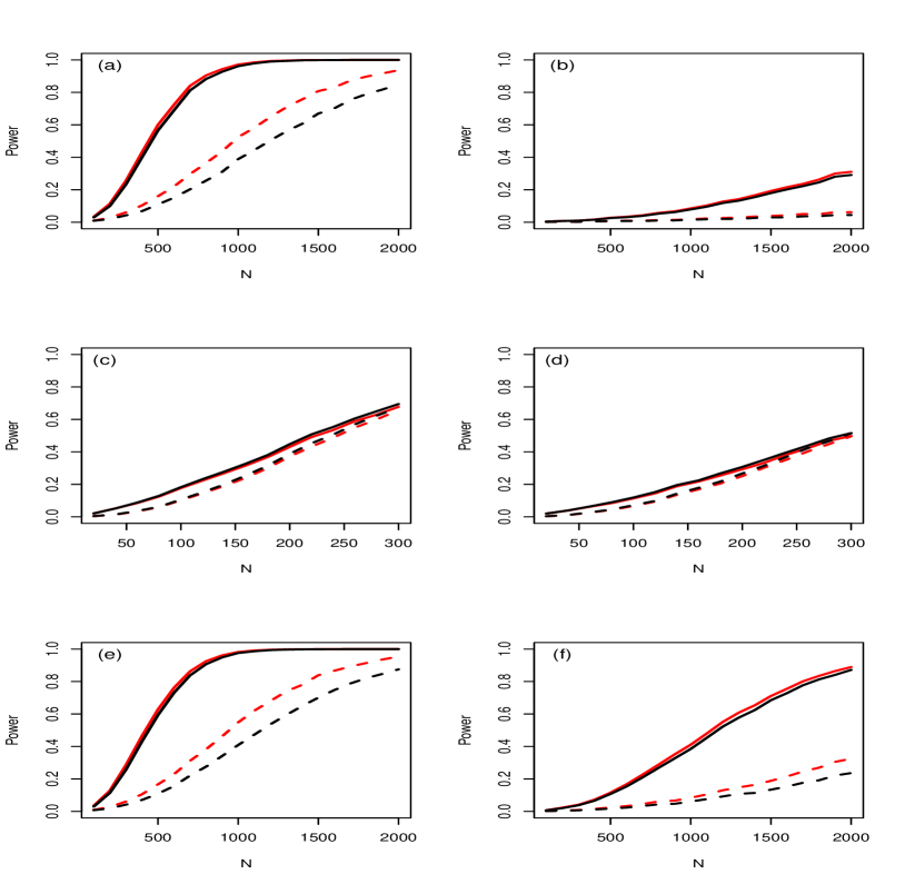
We next evaluate the power of the proposed tests. We consider three different models with $K=3$ groups and repeat the simulation $M=10000$ times. For the first model, we assume that the proportions of zeros are the same across different groups and examine how the distribution of the non-zero observation affects the power of the proposed tests. We set the $\theta=(0.5,0.5,0.5)$ and equal sample sizes for the three groups, chosen from the set $\{100,200,300,\cdots,1900,2000\}$. We set $\alpha\in\{(1.5,2,2.5),(1.7,2,2.3)\}$, and $\beta=(2,2,2)$ and calculate the power function for different sample sizes $N$. The resulting power curves are shown in the top row of Figure 4. We observe a substantial gain in power from the truncated Kruskal-Wallis test.

For the second model, we study how different proportions of zeros affect the test power as the sample size $N$ changes. We set $(\alpha,\beta)=\{(1/2,1/2,1/2),(2,2,2)\}$, which assumes that the nonzero distributions are the same across different groups. We again assume that the sample sizes are the same for all three groups, chosen from the set $\{20,40,60,\cdots,280,300\}$. We set $\theta\in\{(0.1,0.15,0.22),(0.15,0.20,0.27)\}$, and calculate the power function for different sample sizes $N$. The resulting power curves are shown in the middle row of Figure 4. Our test has some improvement over the original test. However, in this case, the improvement is not as large as when $f_{i}$s are different.

For the last model, we evaluate the proposed tests when the sample sizes are different in different groups. We set $\theta=(0.4,0.5,0.6)$ and the sample size as $N\times(0.8,1,1.5)$, where $N\in\{100,200,300,\cdots,1900,2000\}$. We choose $\alpha\in\{(1.5,2,2.5),(1.7,2,2.3)\}$ and $\beta=(2,2,2)$, and calculate the power function for different sample sizes $N$. The power curves are shown in the bottom row of Figure 4, showing that the truncated Kruskal-Wallis test has much higher power than the Kruskal-Wallis test when there are ties.

We finally examine the sensitivity of the proposed tests to reduced sequencing depths. One effect of having low sequencing depth is that some rare bacteria might not be sequenced, which results in zero counts for bacteria with low but non-zero true relative abundance in the final microbial composition. Specifically, after we generate the compositional data for each population, to minic lower sequencing depth, we set the abundance of the bacteria with small relative abundance to zero with a probability of 0.5, resulting about 5% of non-zeros proportions being set to zero. The final data sets include more zeros due to reduced sequencing depths. We obtain the empirical power again based on the final data sets. The new power curves are shown in Figure 4 (red lines). The proposed test still achieve higher power than the standard tests (dashed line). Overall, we see that the proposed tests are not too sensitive to read depths from sequencing.

6 Identifying the Crohn’s disease-associated bacterial genera and the effects of treatment

Crohn’s disease, a chronic inflammatory bowel disease, is characterized by altered composition of the gut microbiota or dysbiosis. The etiology and clinical significance of the dysbiosis is unknown. In a recent study at the University of Pennsylvania, the composition of the gut microbiota among a cohort of 85 children with Crohn’s disease who were initiating therapy with either a defined formula diet ($n$=33) or an anti-tumor necrosis factor $\alpha$ (anti-TNF) drug ($n$=52) was examined in order to better understand the cause of the dysbiosis in Crohn’s disease. Fecal samples were collected at baseline, 1, 4, and 8 weeks and DNA content characterized by shot-gun genomic sequencing with $>$0.5 tetra-bytes of total sequences (Lewis et al., 2015). The gut microbiota data of 26 normal children with no known gastrointestinal disorders were similarly collected. The MetaPhlAn program (Segata et al., 2012) was applied to first obtain the relative proportions of the bacterial genera for each of the normal and Crohn’s disease samples. The number of bacterial genera called by the MetaPhlAn program varied from sample to sample. Altogether, 60 bacterial genera were observed in both healthy samples and the Crohn’s disease samples. Figure 1 shows the relative abundances of the 60 genera in all the samples, where large proportions of zeros are observed for many of the genera.

6.1 Comparison of gut microbiome between normal and Crohn’s disease patients

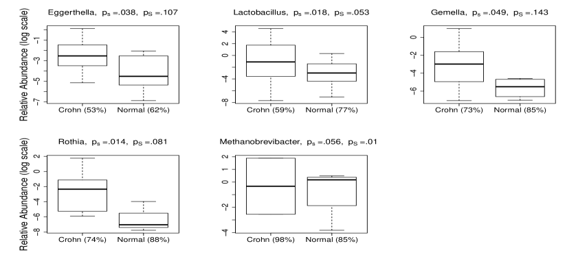
We are interested in identifying the bacterial genera that show different distributions between healthy and Crohn’s disease children. At an $\alpha$ level of 0.05, the truncated Wilcoxon rank-sum test identified 23 genera that showed different distributions between healthy children and patients with Crohn’s disease, while the standard Wilcoxon test identified 20, among these, 19 were identified by both methods. At FDR of 10%, the truncated Wilcoxon rank-sum test identified 21 genera and the standard Wilcoxon test identified the same 20 genera. Four genera, including Eggerthella, Lactobacillus, Gemella, and Rothia were identified only by the truncated Wilcoxon rank-sum test. Figure 5 shows the the proportions of zeros and boxplots of these four genera that clearly show difference in abundances in healthy and Crohn’s disease children, both in terms of proportion of zeros and the median of non-zero abundances. All four genera had higher abundances in Crohn’s patients than the healthy controls. Among these genera, Eggerthella, Lactobacillus, both are anaerobic, non-sporulating, Gram-positive bacilli, have been reported to be associated with clinically significant bacteraemia and Crohn’s disease (Lau et al., 2004). In contrast, for genus Methanobrevibacter, the standard Wilcoxon test had a sightly smaller $p$-value. However, 98% of the disease individuals did not carry this genus. In this case, the truncation may lead to a slightly reduced statistical significance. However, this can also be due to random error or the asymptotic approximation error due to relatively small sample sizes. To verify this, we performed 100,000 permutations of group labels and obtained a p-value of 0.016 and 0.017, for the truncated test and the standard Wilcoxon test, respectively.

Refer to caption
Figure 5: The box plots of the non-zero relative abundances (on log scale) with proportions of zeros in $x$-axis labels for the four bacterial genera that were identified by the truncated Wilcoxon rank-sum test only for a nominal $\alpha$ level of 0.05, where $p$-values from $T_{W}$ and $T_{tW}$ tests are shown as $p_{S}$ and $p_{s}$. The genus Methanobrevibacterm was identified only by the standard Wilcoxon rank-sum test.

6.2 Comparison of gut microbiome across time after treatment

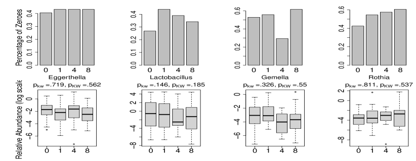
We next aim to identify the bacterial genera that show changes of relative abundances across the four time points during the anti-TNF treatment. We applied our truncated Kruskal-Wallis test statistic with within-subject permutations (100,000 permutations) and identified 7 genera with changes of abundances during the treatment with $p<0.05$. As a comparison, the Friedman’s test identified only three. Figure 6 shows the boxplots of the abundances of the genera across 4 time points for the four genera identified only by our truncated Kruskal-Wallis test, including Bacteroides, Roseburia, Eubacterium and Bilophila. Among these, Bacteroides, Eubacterium and Bilophila showed increased abundances at 8 weeks after the anti-TNF treatment. Interestingly, all three genera have been shown to have reduced abundance in Crohn’s disease patients (Gevers et al., 2014). Reduction of Roseburia, a well-known butyrate-producing bacterium of the Firmicutes phylum, has been consistently demonstrated to be associated with Crohn’s disease (Machiels et al., 2014). There has been evidence that the gut bacteria in patients with inflammatory bowel disease do not make butyrate, and that they have low levels of the fatty acid in their gut (Sartor and Mazmanian, 2012). The decreased abundance of Bilophila, may translate into a reduction of commensal bacteria-mediated, anti-inflammatory activities in the mucosa, which are relevant to the pathophysiology of Crohn’s disease. The result shows the effect of anti-TNF treatment in increasing the relative abundances of Roseburia, Bacteroides and Bilophila, therefore potentially increasing the level of fatty acid butyrate and anti-inflammatory activities. This partially explains that 50% of the patients showed clinical improvement, as reflected by reduction of fecal calprotection below 250 mcg/g (Lewis et al., 2015).

Refer to caption
Figure 6: Bar plots of proportions of zeros (top row) and box plots of the relative non-zero abundances (bottom row, on log scale) over four time points during anti-TNF treatment for four bacteria genera that were identified only by the truncated Kruskal-Wallis test.

7 Discussion

Motivated by comparing the distributions of taxa composition in different groups in microbiome studies, we have developed several extensions of the popular rank-based tests to account for clumps of zeros, including truncated rank-based Wilcoxon and Kruskal-Wallis tests for two- or multiple-group comparisons. These tests are rank-based and nonparametric and are easy to implement. By using within-sample permutations, such tests can also be applied to paired samples or repeated measurements analysis. We have shown that the proposed tests have better power than the standard rank-based tests, both by asymptotic relative efficiency analysis and by simulations. We observed a large gain in power when the proportions of zeros in the data sets are high as compared to the standard rank-based tests due the high number of tied ranks. Hallstrom (2010) showed that the truncated Wilcoxon rank-sum test has equal or better power than the test of two-degree of freedoms based on two-part model when the sample sizes are equal. Since our two-sample truncated test is an extension of Hallstrom’s test to unequal sample sizes, we expect that our proposed tests should have similar or better power than the two-part tests that combine binomial test and nonparametric test for the continuous part. Although such two-part tests can be extended to two-part model for multiple group comparisons, it has not been studied in literature. It would be interesting to compare the performance of our proposed truncated Kruskal-Wallis tests with other tests based on the two-part models.

We have demonstrated the applications of the proposed tests in an analysis of real metagenomic data sets. Our results have shown that the truncated rank-based tests are effective and identify more bacterial genera that are associated with the clinical phenotypes and treatment. As observed in other studies (Wagner, Robertson and Harris, 2011), tests that account for clumps of zeros can be more powerful in testing abundance difference in microbiome studies. We have demonstrated that some well-known Crohn’s disease-associated bacterial genera can be missed by using the standard rank-based tests without adjusting for excessive zeros. We expect to see more applications of the proposed tests in microbiome studies.

The proposed tests have several limitations. First, since these tests are rank-based and nonparametric, they cannot directly account for covariate effects in observational studies. If there is no severe covariate imbalance, we can perform quantile-stratification based on covariates and apply the proposed tests to each strata and then combine the results using e.g., Fisher’s combination of $p$-values. This requires large sample sizes. Second, since the $p$-values of our proposed rank-based tests are calculated based on the asymptotic distributions of the test statistics, which require relatively large sample sizes, they may not be accurate enough when the sample sizes are small. As shown in our Table 1, as the sample sizes increase, the Type I error gets closer to the nominal level. For small sample sizes, we would suggest that the users apply the proposed tests and obtain the $p$-values based the asymptotic distributions. Once the taxa are identified, one can run a permutation test to further confirm the results. This will save time to run permutation tests for all the taxa.

Acknowledgment

This research was supported by NIH grants GM129781 and GM123056. We thank Dr. Kafadar, the AE and two reviewers for many helpful comments and suggestions.

SUPPLEMENTARY MATERIALS

The online Supplemental Materials include proofs of Theorem 1, Theorem 2 and all the lemmas. It also includes detailed derivations of the proposed test statistics and simulations to verify the theoretical asymptotic relative efficiency of the proposed tests. An R repository of the proposed method and all analyses performed is available at https://github.com/hongzhe88/Truncated-Rank-based-Tests.

References

  • Gevers et al. (2014) {barticle}[author] \bauthor\bsnmGevers, \bfnmDirk\binitsD., \bauthor\bsnmKugathasan, \bfnmSubra\binitsS., \bauthor\bsnmDenson, \bfnmLee A.\binitsL. A. and \bauthor\bparticleet \bsnmal (\byear2014). \btitleThe treatment-naive microbiome in new-onset Crohn’s disease. \bjournalCell Host & Microbe \bvolume15 \bpages382–392. \endbibitem
  • Hallstrom (2010) {barticle}[author] \bauthor\bsnmHallstrom, \bfnmAP\binitsA. (\byear2010). \btitleA modified Wilcoxon test for non-negative distributions with a clump of zeros. \bjournalStatistics in Medicine \bvolume29 \bpages391–400. \endbibitem
  • Huson et al. (2007) {barticle}[author] \bauthor\bsnmHuson, \bfnmDaniel H\binitsD. H., \bauthor\bsnmAuch, \bfnmAlexander F\binitsA. F., \bauthor\bsnmQi, \bfnmJi\binitsJ. and \bauthor\bsnmSchuster, \bfnmStephan C\binitsS. C. (\byear2007). \btitleMEGAN analysis of metagenomic data. \bjournalGenome research \bvolume17 \bpages377–386. \endbibitem
  • Lachenbruch (1976) {barticle}[author] \bauthor\bsnmLachenbruch, \bfnmP\binitsP. (\byear1976). \btitleAnalysis of Data with Clumping at Zero. \bjournalBiometrische Zeitschrift \bvolume18 \bpages351–356. \endbibitem
  • Lachenbruch (2001) {barticle}[author] \bauthor\bsnmLachenbruch, \bfnmP\binitsP. (\byear2001). \btitleComparison of two-part models with competitors. \bjournalStatistics in Medicine \bvolume20 \bpages1215–1234. \endbibitem
  • Lachenbruch (2002) {barticle}[author] \bauthor\bsnmLachenbruch, \bfnmPeter A\binitsP. A. (\byear2002). \btitleAnalysis of data with excess zeros. \bjournalStatistical methods in medical research \bvolume11 \bpages297–302. \endbibitem
  • Lau et al. (2004) {barticle}[author] \bauthor\bsnmLau, \bfnmS\binitsS., \bauthor\bsnmWoo, \bfnmP\binitsP., \bauthor\bsnmFung, \bfnmA\binitsA., \bauthor\bsnmChan, \bfnmKM\binitsK., \bauthor\bsnmWoo, \bfnmG\binitsG. and \bauthor\bsnmYuen, \bfnmKY\binitsK. (\byear2004). \bjournalJournal of Medical Microbiology \bvolume53 \bpages1247–1253. \endbibitem
  • Lewis et al. (2015) {barticle}[author] \bauthor\bsnmLewis, \bfnmJD\binitsJ., \bauthor\bsnmChen, \bfnmE. Z.\binitsE. Z., \bauthor\bsnmBaldassano, \bfnmR. N.\binitsR. N., \bauthor\bsnmOtley, \bfnmA. R.\binitsA. R., \bauthor\bsnmGriffiths, \bfnmA. M.\binitsA. M., \bauthor\bsnmLee, \bfnmD.\binitsD., \bauthor\bsnmBittinger, \bfnmK.\binitsK., \bauthor\bsnmBailey, \bfnmA.\binitsA., \bauthor\bsnmFriedman, \bfnmE. S.\binitsE. S., \bauthor\bsnmHoffmann, \bfnmC.\binitsC., \bauthor\bsnmAlbenberg, \bfnmL.\binitsL., \bauthor\bsnmSinha, \bfnmR.\binitsR., \bauthor\bsnmCompher, \bfnmC.\binitsC., \bauthor\bsnmGilroy, \bfnmE.\binitsE., \bauthor\bsnmNessel, \bfnmL.\binitsL., \bauthor\bsnmGrant, \bfnmA.\binitsA., \bauthor\bsnmChehoud, \bfnmC\binitsC., \bauthor\bsnmLi, \bfnmH.\binitsH., \bauthor\bsnmWu, \bfnmG. D.\binitsG. D. and \bauthor\bsnmBushman, \bfnmF. D.\binitsF. D. (\byear2015). \btitleInflammation, Antibiotics, and Diet as Environmental Stressors of the Gut Microbiome in Pediatric Crohn’s Disease. \bjournalCell Host & Microbe \bvolume18 \bpages489-500. \endbibitem
  • Machiels et al. (2014) {barticle}[author] \bauthor\bsnmMachiels, \bfnmK\binitsK., \bauthor\bsnmJoossens, \bfnmM\binitsM., \bauthor\bsnmSabino, \bfnmJ\binitsJ., \bauthor\bsnmDe Preter, \bfnmV\binitsV., \bauthor\bsnmArijs, \bfnmI\binitsI., \bauthor\bsnmEeckhaut, \bfnmV\binitsV., \bauthor\bsnmBallet, \bfnmV\binitsV., \bauthor\bsnmClaes, \bfnmK\binitsK., \bauthor\bsnmVan Immerseel, \bfnmF\binitsF., \bauthor\bsnmVerbeke, \bfnmK\binitsK., \bauthor\bsnmFerrante, \bfnmM\binitsM., \bauthor\bsnmVerhaegen, \bfnmJ\binitsJ., \bauthor\bsnmRutgeerts, \bfnmP\binitsP. and \bauthor\bsnmVermeire, \bfnmS\binitsS. (\byear2014). \btitleA decrease of the butyrate-producing species Roseburia hominis and Faecalibacterium prausnitzii defines dysbiosis in patients with ulcerative colitis. \bjournalGut \bvolume63(8) \bpages1275–1283. \endbibitem
  • Manichanh et al. (2012) {barticle}[author] \bauthor\bsnmManichanh, \bfnmChaysavanh\binitsC., \bauthor\bsnmBorruel, \bfnmNatalia\binitsN., \bauthor\bsnmCasellas, \bfnmFrancesc\binitsF. and \bauthor\bsnmGuarner, \bfnmFrancisco\binitsF. (\byear2012). \btitleThe gut microbiota in IBD. \bjournalNature Reviews Gastroenterology and Hepatology \bvolume9 \bpages599–608. \endbibitem
  • Qin et al. (2010) {barticle}[author] \bauthor\bsnmQin, \bfnmJunjie\binitsJ., \bauthor\bsnmLi, \bfnmRuiqiang\binitsR., \bauthor\bsnmRaes, \bfnmJeroen\binitsJ., \bauthor\bsnmArumugam, \bfnmManimozhiyan\binitsM., \bauthor\bsnmBurgdorf, \bfnmKristoffer Solvsten\binitsK. S., \bauthor\bsnmManichanh, \bfnmChaysavanh\binitsC., \bauthor\bsnmNielsen, \bfnmTrine\binitsT., \bauthor\bsnmPons, \bfnmNicolas\binitsN., \bauthor\bsnmLevenez, \bfnmFlorence\binitsF., \bauthor\bsnmYamada, \bfnmTakuji\binitsT. \betalet al. (\byear2010). \btitleA human gut microbial gene catalogue established by metagenomic sequencing. \bjournalNature \bvolume464 \bpages59–65. \endbibitem
  • Qin et al. (2012) {barticle}[author] \bauthor\bsnmQin, \bfnmJunjie\binitsJ., \bauthor\bsnmLi, \bfnmYingrui\binitsY., \bauthor\bsnmCai, \bfnmZhiming\binitsZ., \bauthor\bsnmLi, \bfnmShenghui\binitsS., \bauthor\bsnmZhu, \bfnmJianfeng\binitsJ., \bauthor\bsnmZhang, \bfnmFan\binitsF., \bauthor\bsnmLiang, \bfnmSuisha\binitsS., \bauthor\bsnmZhang, \bfnmWenwei\binitsW., \bauthor\bsnmGuan, \bfnmYuanlin\binitsY., \bauthor\bsnmShen, \bfnmDongqian\binitsD. \betalet al. (\byear2012). \btitleA metagenome-wide association study of gut microbiota in type 2 diabetes. \bjournalNature \bvolume490 \bpages55–60. \endbibitem
  • Sartor and Mazmanian (2012) {barticle}[author] \bauthor\bsnmSartor, \bfnmRB\binitsR. and \bauthor\bsnmMazmanian, \bfnmSK\binitsS. (\byear2012). \btitleIntestinal Microbes in Inflammatory Bowel Diseases. \bjournalAmerican Journal of Gastroenterology (Supplements) \bvolume1 \bpages15-21. \endbibitem
  • Segata et al. (2012) {barticle}[author] \bauthor\bsnmSegata, \bfnmNicola\binitsN., \bauthor\bsnmWaldron, \bfnmLevi\binitsL., \bauthor\bsnmBallarini, \bfnmAnnalisa\binitsA., \bauthor\bsnmNarasimhan, \bfnmVagheesh\binitsV., \bauthor\bsnmJousson, \bfnmOlivier\binitsO. and \bauthor\bsnmHuttenhower, \bfnmCurtis\binitsC. (\byear2012). \btitleMetagenomic microbial community profiling using unique clade-specific marker genes. \bjournalNature Methods \bvolume9 \bpages811–814. \endbibitem
  • Turnbaugh et al. (2006) {barticle}[author] \bauthor\bsnmTurnbaugh, \bfnmPeter J\binitsP. J., \bauthor\bsnmLey, \bfnmRuth E\binitsR. E., \bauthor\bsnmMahowald, \bfnmMichael A\binitsM. A., \bauthor\bsnmMagrini, \bfnmVincent\binitsV., \bauthor\bsnmMardis, \bfnmElaine R\binitsE. R. and \bauthor\bsnmGordon, \bfnmJeffrey I\binitsJ. I. (\byear2006). \btitleAn obesity-associated gut microbiome with increased capacity for energy harvest. \bjournalNature \bvolume444 \bpages1027–131. \endbibitem
  • Turnbaugh et al. (2007) {barticle}[author] \bauthor\bsnmTurnbaugh, \bfnmPeter J\binitsP. J., \bauthor\bsnmLey, \bfnmRuth E\binitsR. E., \bauthor\bsnmHamady, \bfnmMicah\binitsM., \bauthor\bsnmFraser-Liggett, \bfnmClaire M\binitsC. M., \bauthor\bsnmKnight, \bfnmRob\binitsR. and \bauthor\bsnmGordon, \bfnmJeffrey I\binitsJ. I. (\byear2007). \btitleThe human microbiome project. \bjournalNature \bvolume449 \bpages804–810. \endbibitem
  • Wagner, Robertson and Harris (2011) {barticle}[author] \bauthor\bsnmWagner, \bfnmBD\binitsB., \bauthor\bsnmRobertson, \bfnmCE\binitsC. and \bauthor\bsnmHarris, \bfnmJK\binitsJ. (\byear2011). \btitleApplication of Two–Part Statistics for Comparison of Sequence Variant Counts. \bjournalPloS One \bvolume6(5) \bpagese20296. \endbibitem

Appendix A Simulations on ARE$(T_{tKW},T_{KW})$

In Theorem 1, we derived the theoretical results of $\textsc{are}(T_{tKW},T_{KW})$ and presented how it relates to different parameters in Figure 2. In this section, we present simulation results to further verify the theoretial results presented in Figure 2.

For each of the 4 settings, we calculated the are by empirical means and variances of the test statistics under null and alternatives based on 10,000 simulations. The four settings are almost the same with that in Figure 2, except some extreme values that are hard to realize in numerical studies.

  • (a)

    Effect of $\Delta_{f,g}$: $N_{1}=40$, and $N_{2}=50$ and $\theta_{1}=0.3$, $\theta_{2}=0.8$. Let $\Delta_{f,g}{=-0.5+0.01k}$, where $k=3,4,5,\cdots,98$. For each choice $\delta=\Delta_{f,g}$, we take $f\sim Beta(3,3)$, and $g\sim Beta(\alpha,\beta)$, where $1<\alpha<10$ and $1<\beta<10$ are chosen so that $|\Delta_{f,g}-\delta|<0.05$.

  • (b)

    Effect of $\theta$: $N_{1}=40$, $N_{2}=50$, $f\sim Beta(2,2.75)$, and $g\sim Beta(2,2)$. Note that $\Delta_{f,g}=0.10$ with current choice of $f$ and $g$. Let $\theta=0.1+0.01k$, where $k=0,1,2,\cdots,80$. With a given $\theta$, take $\theta_{1}=\theta-0.1$ and $\theta_{2}=\theta+0.1$.

  • (c)

    Effect of $\triangle\theta$: $N_{1}=40$, $N_{2}=50$, $f\sim Beta(2,2.75)$, and $g\sim Beta(2,2)$. Note that $\Delta_{f,g}=0.10$ with current choice of $f$ and $g$. Let $\triangle\theta=0.02k$, where $k=1,2,\cdots,45$. With a given $\triangle\theta$, take $\theta_{1}=0.5-\triangle\theta/2$ and $\theta_{2}=0.5+\triangle\theta/2$.

  • (d)

    Effect of sample size: $\theta_{1}=0.3$, $\theta_{2}=0.8$, $f\sim Beta(2,2.75)$, and $g\sim Beta(2,2)$. Note that $\Delta_{f,g}=0.10$ with current choice of $f$ and $g$. Let $N_{2}=50$, and choose $N_{1}\in\{20,25,30,\cdots,115,120\}$.

We observe that the simulated are is close to the theoretical are, in terms of both values and the trends as we change the parameters. For setting (d), the theoretical line is flat while the simulated line is not flat. The reason is there is an additional term $O(|N_{2}-N_{1}|)$ in the formula, see (12). It has a low order compared to $N_{1}N_{2}$, so it was ignored in the main term. The theoretical curve corresponds to the main term, which does not depend on $N_{1}$, but the simulated curve also takes this remainder term into account.

Refer to caption
Figure 7: The theoretical (black) and simulated (red) asymptotic relative efficiency $\textsc{are}(T_{tW},T_{W})$ comparing the truncated Wilcoxon rank test and the standard Wilcoxon rank test as a function of (a) $\Delta_{f,g}$, (b) $\theta$, (c) $\triangle\theta$, and (d) $N_{1}$. For each plot, the horizontal dashed line represents $\textsc{are}(T_{tW},T_{W})=1$.

Appendix B Basic properties

Suppose there is a sample with size $n$. Rank all the observations so that the smallest observations have largest ranks. Let $r_{i}$ and $r_{j}$ denote the ranks of two randomly selected observations. We have the results for the expectation, variance and covariance as follows. The calculations are also presented here although its basic in statistics.

Property 1. $\mathrm{E}[r_{i}]=\frac{n+1}{2}$.

Property 2. $\mathrm{E}[r_{i}^{2}]=\frac{(n+1)(2n+1)}{6}$.

Proof. $\mathrm{E}[r_{i}^{2}]=\frac{1}{n}\sum_{i=1}^{n}i^{2}=\frac{(n+1)(2n+1)}{6}$.

Property 3. $\mathrm{Var}[r_{i}]=\frac{n^{2}-1}{12}$.

Proof. Note that $\mathrm{Var}(r_{i})=\mathrm{E}[r_{i}^{2}]-(E[r_{i}])^{2}$. According to Properties 1–2, the variance is

$$\mathrm{Var}(r_{i})=\frac{1}{n}\sum_{i=1}^{n}i^{2}-(\frac{n+1}{2})^{2}=\frac{n^{2}-1}{12}.$$

Property 4. $\mathrm{Cov}[r_{i},r_{j}]=-\frac{n+1}{12}$.

Proof. When $i\neq j$, we have

$$\mathrm{E}[r_{i}r_{j}]=\frac{1}{n(n-1)}\sum_{i\neq j}ij=\frac{(n+1)(3n+2)}{12}.$$

Therefore,

$$\mathrm{Cov}(r_{i},r_{j})=\mathrm{E}[r_{i}r_{j}]-[\mathrm{E}(r_{i})]^{2}=\frac{(n+1)(3n+2)}{12}-(\frac{n+1}{2})^{2}=-\frac{n+1}{12}.$$

Property 5. Consider a randomly selected group of observations $S$ with size $n_{1}$. The rank-sum of this group is denoted by $r_{g}$. Then,

$$\mathrm{E}[r_{g}]=\frac{1+n}{2}n_{1},\qquad\mathrm{Var}(r_{g})=\frac{n_{1}(n-n_{1})(n+1)}{12}.$$

Proof. For the expectation part, it simply introduces in $E[r_{i}]$ for each observation in this group. Next we check the variance.

$\displaystyle\mathrm{Var}(r_{g})$ $\displaystyle=$ $\displaystyle\sum_{i\in S}\mathrm{Var}(r_{i})+\sum_{i,j\in S,i\neq j}\mathrm{Cov}(r_{i},r_{j})$
$\displaystyle=$ $\displaystyle\sum_{i\in S}\frac{n^{2}-1}{12}+\sum_{i,j\in S,i\neq j}-\frac{n+1}{12}$
$\displaystyle=$ $\displaystyle\frac{n_{1}(n-n_{1})(n+1)}{12}.$

Appendix C Derivations of the Modified Wilcoxon Rank Sum Statistic

For a given statistic $S$, we use ${\mathrm{E}}[S]$ and ${\mathrm{Var}}(S)$ to represent its mean and variance calculated under the null hypothesis and use ${\mathrm{E}}_{1}[S]$ to represent its mean calculated under the alternative hypothesis. In this section, given that $W=S^{2}/{\mathrm{Var}}(S)$ where $S=R-\frac{N_{1}+N_{2}+1}{2}N_{1}$, and $s=r-\frac{\lfloor p(N_{1}+N_{2})\rfloor+1}{2}\lfloor pN_{1}\rfloor-\frac{1}{4}\frac{p_{1}+p_{2}}{2}(1-\frac{p_{1}+p_{2}}{2})(N_{2}-N_{1})$, we want to verify the following results:

  • ${\mathrm{E}}[S]=0$, ${\mathrm{E}}[s]=O(\max\{N_{1},N_{2}\})$;

  • the results for ${\mathrm{Var}}(S)$ and ${\mathrm{Var}}(s)$:

    $\displaystyle\mathrm{Var}(S)$ $\displaystyle=$ $\displaystyle N_{1}N_{2}(N_{1}+N_{2})\theta(1-\theta+\theta^{2}/3)/4+O(N^{2.5}),$
    $\displaystyle\mathrm{Var}(s)$ $\displaystyle=$ $\displaystyle N_{1}N_{2}(N_{1}+N_{2})\theta^{3}(1-\theta+1/3)/4+O(N^{2.5});$

Proof. Now we prove the results one by one.

  • We show the expectation first. The result for ${\mathrm{E}}[S]$ is direct, so we focus on ${\mathrm{E}}[s]$.

    Recall that $p=\max\{p_{1},p_{2}\}$, where $p_{1}=n_{1}/N_{1}$ and $p_{2}=n_{2}/N_{2}$. Let $\tilde{r}=r-\frac{\lfloor p(N_{1}+N_{2})\rfloor+1}{2}\lfloor pN_{1}\rfloor$, and so $s=\tilde{r}-\frac{1}{4}\frac{p_{1}+p_{2}}{2}(1-\frac{p_{1}+p_{2}}{2})(N_{2}-N_{1})$. To find $E[s]$, we need to calculate $E[\tilde{r}]$ and $E[\frac{1}{4}\frac{p_{1}+p_{2}}{2}(1-\frac{p_{1}+p_{2}}{2})(N_{2}-N_{1})]$.

    With independent samples, $p_{1}$ and $p_{2}$ are independent, ${\mathrm{E}}[p_{i}]=\theta_{i}$ and ${\mathrm{Var}}(p_{i})=\theta_{i}(1-\theta_{i})/N_{i})$, $i=1,2$. Under null hypothesis, $\theta_{1}=\theta_{2}=\theta$. We then have

    $\displaystyle E\biggl{[}\frac{1}{4}\frac{p_{1}+p_{2}}{2}(1-\frac{p_{1}+p_{2}}{2})(N_{2}-N_{1})\biggr{]}$ $\displaystyle=$ $\displaystyle\frac{N_{2}-N_{1}}{4}\biggl{[}(\frac{\theta_{1}+\theta_{2}}{2})-(\frac{\theta_{1}+\theta_{2}}{2})^{2}-\frac{\theta_{1}(1-\theta_{1})}{4N_{1}}-\frac{\theta_{2}(1-\theta_{2})}{4N_{2}}\biggr{]}$
    $\displaystyle\mbox{(Let }\theta=\frac{\theta_{1}+\theta_{2}}{2})\qquad$ $\displaystyle=$ $\displaystyle\frac{N_{2}-N_{1}}{4}(\theta(1-\theta)+O(\frac{1}{N_{1}}+\frac{1}{N_{2}})).$ (7)

    Here, $\theta$ is the probability of zero under null and $\theta=(\theta_{1}+\theta_{2})/2$ under alternative hypothesis.

    Next we calculate $E[\tilde{r}]$. Recall that $r$ is the sum-rank of the truncated sample 1. Let $r_{0}$ be the sum-rank of all the non-zero elements in the truncated sample 1. With $r_{0}$, we rewrite $\tilde{r}$ as

    $\displaystyle\tilde{r}$ $\displaystyle=$ $\displaystyle r_{0}-\frac{n_{1}+n_{2}+1}{2}n_{1}+\frac{n_{1}+n_{2}+1+\lfloor p(N_{1}+N_{2})\rfloor}{2}(\lfloor pN_{1}\rfloor-n_{1})$
    $\displaystyle-\frac{1+\lfloor p(N_{1}+N_{2})\rfloor}{2}\lfloor pN_{1}\rfloor+\frac{n_{1}+n_{2}+1}{2}n_{1}$
    $\displaystyle=$ $\displaystyle(r_{0}-\frac{n_{1}+n_{2}+1}{2}n_{1})+\frac{1}{2}pN_{1}N_{2}(p_{2}-p_{1})+O(\max\{N_{1},N_{2}\}),$

    where $O(N_{2})$ comes from the difference between $\lfloor pN_{1}\rfloor$ ($\lfloor pN_{1}\rfloor$) and $pN_{1}$ ($pN_{2}$).

    Since all the observations are non-negative, so the non-zero elements always enjoy the ranks from 1 to $n_{1}+n_{2}$. Hence, under null hypothesis that $f=g$, $E[r_{0}-\frac{n_{1}+n_{2}+1}{2}n_{1}]=0$. Therefore,

    $${\mathrm{E}}[\tilde{r}|p_{1},p_{2}]=\frac{pN_{1}N_{2}}{2}(p_{2}-p_{1})+O(\max\{N_{1},N_{2}\}).$$ (8)

    We still need to remove the condition that $p_{1}$ and $p_{2}$ are given. The following lemma is used to describe the distribution of $p(p_{2}-p_{1})$.

    Lemma A.

    Define $p_{1}=n_{1}/N_{1}$, $p_{2}=n_{2}/N_{2}$, and $p=\max\{p_{1},p_{2}\}$. Under null hypothesis that $\theta_{1}=\theta_{2}=\theta$, $F=G$, and let $N_{1},N_{2}\rightarrow\infty$ at the same order, there is

    $\displaystyle E[p(p_{2}-p_{1})/2]=\frac{\theta(1-\theta)}{4}\frac{N_{1}-N_{2}}{N_{1}N_{2}},$
    $\displaystyle E[p^{2}(p_{2}-p_{1})^{2}]=\theta^{3}(1-\theta)(1/N_{1}+1/N_{2})+O(N_{1}^{-3/2}).$

    Combining Lemma A with (8) leads to

    $$E[\tilde{r}]=\frac{\theta(1-\theta)}{4}(N_{1}-N_{2})+O(\max\{N_{1},N_{2}\}).$$

    Combining this with (C), we have that

    $$E[s]=O(\max\{N_{1},N_{2}\}).$$

    The first conclusion is proved.

  • Next we want to check ${\mathrm{Var}}(S)$ and ${\mathrm{Var}}(s)$.

    Note that $s=\tilde{r}-\frac{1}{4}\frac{p_{1}+p_{2}}{2}(1-\frac{p_{1}+p_{2}}{2})(N_{2}-N_{1})=\tilde{r}-I$. Therefore,

    $${\mathrm{Var}}(s)={\mathrm{Var}}(\tilde{r})+{\mathrm{Var}}(I)-2{\mathrm{Cov}}(\tilde{r},I).$$ (9)

    Check the terms one by one.

    The first term is ${\mathrm{Var}}(\tilde{r})$. Note that we already find ${\mathrm{E}}[\tilde{r}|p_{1},p_{2}]=pN_{1}N_{2}(p_{2}-p_{1})/2+O(\max\{N_{1},N_{2}\})$. Therefore,

    $\displaystyle{\mathrm{Var}}(\tilde{r})$ $\displaystyle=$ $\displaystyle{\mathrm{Var}}({\mathrm{E}}[\tilde{r}|p_{1},p_{2}])+{\mathrm{E}}[{\mathrm{Var}}(\tilde{r}|p_{1},p_{2})]$
    $\displaystyle=$ $\displaystyle\frac{N_{1}^{2}N_{2}^{2}}{4}\{E[(p_{2}-p_{1})^{2}p^{2}]-(E[(p_{2}-p_{1})p])^{2}\}+\frac{N_{1}N_{2}}{12}E[N_{1}p_{1}^{2}p_{2}+N_{2}p_{1}p_{2}^{2}+p_{1}p_{2}].$

    With Lemma A we have that

    $\displaystyle E[(p_{2}-p_{1})^{2}p^{2}]=\theta^{3}(1-\theta)(1/N_{1}+1/N_{2})+O(N_{1}^{-3/2}),$
    $\displaystyle(E[(p_{2}-p_{1})p])^{2}=\theta^{2}(1-\theta)^{2}(N_{1}-N_{2})^{2}/(4N_{1}^{2}N_{2}^{2})=O(N_{1}^{-2}).$

    Combining with $E[N_{1}p_{1}^{2}p_{2}+N_{2}p_{1}p_{2}^{2}+p_{1}p_{2}]=(N_{1}+N_{2})\theta^{3}+O(1)$ from basic statistics, we have that

    $${\mathrm{Var}}(\tilde{r})=N_{1}N_{2}(N_{1}+N_{2})\theta^{3}(1-\theta+1/3)/4+O(\sqrt{N_{1}}N_{2}^{2}).$$ (10)

    For the second term, note that

    $${\mathrm{Var}}(I)\leq E[I^{2}]\leq(N_{2}-N_{1})^{2}E[(\frac{1}{4}\frac{p_{1}+p_{2}}{2}(1-\frac{p_{1}+p_{2}}{2}))^{2}]\leq(N_{2}-N_{1})^{2}=O(N^{2}),$$

    and

    $${\mathrm{Cov}}(\tilde{r},I)\leq\sqrt{{\mathrm{Var}}(\tilde{r}),{\mathrm{Var}}(I)}\leq(N_{2}-N_{1})\sqrt{N_{1}N_{2}(N_{1}+N_{2})}=O(N^{5/2}).$$

    Introduce the result and (10) into (9), we have

    $${\mathrm{Var}}(s)={\mathrm{Var}}(\tilde{r})+{\mathrm{Var}}(I)-2{\mathrm{Cov}}(\tilde{r},I)=N_{1}N_{2}(N_{1}+N_{2})\theta^{3}(1-\theta+1/3)/4+O(N^{2.5}).$$ (11)

    Similarly, we have that ${\mathrm{Var}}(S)=N_{1}N_{2}(N_{1}+N_{2})\theta(1-\theta+\theta^{2}/3)/4+O(N^{2.5})$.

Appendix D Proof of Theorem 1 in main paper

Recall that the definition of $\textsc{are}(W_{m},W)$ is

$$\textsc{are}(W_{m},W)=\frac{{\mathrm{E}}[s^{2}]/{\mathrm{Var}}(s)}{{\mathrm{E}}_{1}[S^{2}]/{\mathrm{Var}}(S)},$$

where ${\mathrm{E}}_{1}$ denote the expectation under alternative hypothesis, and ${\mathrm{Var}}(s)$ means the variance of $s$ under null hypothesis. With previous analysis, ${\mathrm{Var}}(s)$ and ${\mathrm{Var}}(S)$ are known. The remaining problem is ${\mathrm{E}}_{1}[s^{2}]$, for which we can derive ${\mathrm{E}}_{1}[s]$ and ${\mathrm{Var}}_{1}(s)$ separately, and the combine them together. Here, ${\mathrm{Var}}_{1}(s)$ denote the variance of $s$ under alternative hypothesis.

Recall that we rewrite $s=\tilde{r}-I$, where $\tilde{r}$ can be rewritten as

$$\tilde{r}=[r_{0}-\frac{n_{1}+n_{2}+1}{2}n_{1}]+\frac{1}{2}pN_{1}N_{2}(p_{2}-p_{1})+O(N_{2}).$$

Since $r_{0}$ depend on the non-zero part only, so we only consider the non-zero elements of $\mathbf{x}$ and $\mathbf{y}$. Let $\mathbf{x}(j)$ and $\mathbf{y}(j)$ denote the $j$th non-zero observation in $\mathbf{x}$ and $\mathbf{y}$, respectively. The rank of $\mathbf{x}(j)$ equals to

$$r_{j}=\frac{1}{2}+\sum_{m=1}^{n_{1}}1\{\mathbf{x}(j)<\mathbf{x}(m)\}+\sum_{m=1}^{n_{2}}1\{\mathbf{x}(j)<\mathbf{y}(m)\}+\frac{1}{2}\sum_{m=1}^{n_{1}}1\{\mathbf{x}(j)=\mathbf{x}(m)\}+\frac{1}{2}\sum_{m=1}^{n_{2}}1\{\mathbf{x}(j)=\mathbf{x}(m)\}.$$

Note that ${\mathrm{E}}[1\{\mathbf{x}(j)<\mathbf{x}(m)\}]=P(X_{1}<X_{2})$ when $X_{1},X_{2}\stackrel{{\scriptstyle i.i.d.}}{{\sim}}f$, and $E[1\{\mathbf{x}(j)<\mathbf{y}(m)\}]=P(X<Y)$ when $X\sim f,Y\sim g$ independently. Therefore, we have

$${\mathrm{E}}_{1}[r_{j}|n_{1},n_{2}]=1/2+n_{1}P(X_{1}<X_{2})+n_{2}P(X<Y)+\frac{n_{1}}{2}P(X_{1}=X_{2})+\frac{n_{2}}{2}P(X=Y).$$

Note that $P(X_{1}=X_{2})/2+P(X_{1}<X_{2})=1/2$ since they follow the same distribution and $P(X=Y)/2+P(X<Y)=\Delta_{f,g}+1/2$ according to the definition, plug them in and we have that

$${\mathrm{E}}_{1}[r_{0}|n_{1},n_{2}]={\mathrm{E}}_{1}\biggl{[}\sum_{j=1}^{n_{1}}r_{1j}\biggr{]}=n_{1}\biggl{[}(n_{1}+1)/2+n_{2}[\Delta_{f,g}+1/2]\biggr{]}.$$

Introduce it into the definition of $\tilde{r}$, we have

$${\mathrm{E}}_{1}[\tilde{r}|n_{1},n_{2}]={\mathrm{E}}_{1}[r_{0}|n_{1},n_{2}]-\frac{n_{1}+n_{2}+1}{2}n_{1}+\frac{1}{2}pN_{1}N_{2}(p_{2}-p_{1})=n_{1}n_{2}\Delta_{f,g}+\frac{1}{2}pN_{1}N_{2}(p_{2}-p_{1}).$$

Further, let $N_{1},N_{2}\rightarrow\infty$, and note that $n_{1}\sim Binomial(N_{1},\theta_{1})$, $n_{2}\sim Binomial(N_{2},\theta_{2})$, we have that

$${\mathrm{E}}_{1}[\tilde{r}]=\theta_{1}\theta_{2}N_{1}N_{2}\Delta_{f,g}+\frac{1}{2}\theta_{(m)}N_{1}N_{2}\Delta\theta,$$

For the last term $I$, note that $|{\mathrm{E}}_{1}[I]|<N_{2}-N_{1}=O(N)$. Combining all these terms, we have that

$${\mathrm{E}}_{1}[s]={\mathrm{E}}_{1}[\tilde{r}]-{\mathrm{E}}[I]=\theta_{1}\theta_{2}N_{1}N_{2}\Delta_{f,g}+\frac{1}{2}\theta_{(m)}N_{1}N_{2}\Delta\theta+O(N).$$ (12)

Similarly, we have the result for $S$ as

$\displaystyle{\mathrm{E}}_{1}[S]$ $\displaystyle=$ $\displaystyle{\mathrm{E}}_{1}\biggl{[}{\mathrm{E}}_{1}[r_{0}|n_{1},n_{2}]+\frac{n_{1}+n_{2}+1+N_{1}+N_{2}}{2}(N_{1}-n_{1})-\frac{N_{1}+N_{2}+1}{2}N_{1}\biggr{]}$ (13)
$\displaystyle=$ $\displaystyle{\mathrm{E}}_{1}\bigl{[}n_{1}n_{2}\Delta_{f,g}+\frac{N_{1}n_{2}-n_{1}N_{2}}{2}\bigr{]}$
$\displaystyle=$ $\displaystyle\theta_{1}\theta_{2}N_{1}N_{2}\Delta_{f,g}+\frac{1}{2}N_{1}N_{2}\Delta\theta.$

Now we consider the variance under alternative hypothesis. We deal with $S$ first.

Note that $S$ is a function of all the observations $\mathbf{x}$ and $\mathbf{y}$. To find the variance, we try to bound $P(|S-\mu|\geq t)$ for any $t$ with concentration inequality. When one observation of $\mathbf{x}$ changes, the largest change of $S$ caused by it is $N_{2}$. When one observation of $\mathbf{y}$ changes, the largest change of $S$ is $N_{1}$. Mathematically, we have

$\displaystyle|S(x(1),\cdots,x(k),\cdots,x(N_{1}),\mathbf{y})-S(x(1),\cdots,x^{\prime}(k),\cdots,x(N_{1}),\mathbf{y})|$ $\displaystyle\leq$ $\displaystyle N_{2},$
$\displaystyle|S(\mathbf{x},y(1),\cdots,y(k),\cdots,y(N_{2}))-S(\mathbf{x},y(1),\cdots,y^{\prime}(k),\cdots,y(N_{2}))|$ $\displaystyle\leq$ $\displaystyle N_{1}.$

According to McDiarmid’s Inequality (McDiarmid, Page 206), there is

$$P(|S-{\mathrm{E}}[S]|>t)\leq 2e^{\frac{-2t^{2}}{N_{1}N_{2}^{2}+N_{2}N_{1}^{2}}}.$$

Therefore,

$\displaystyle{\mathrm{Var}}_{1}(S)$ $\displaystyle=$ $\displaystyle{\mathrm{E}}[|S-{\mathrm{E}}[S]|^{2}]=\int_{0}^{\infty}P(|S-{\mathrm{E}}(S)|^{2}\geq t)dt$
$\displaystyle=$ $\displaystyle\int_{0}^{\infty}P(|S-{\mathrm{E}}(S)|\geq\sqrt{t})dt$
$\displaystyle\leq$ $\displaystyle\int_{0}^{\infty}2e^{\frac{-2t}{N_{1}N_{2}^{2}+N_{2}N_{1}^{2}}}dt$
$\displaystyle=$ $\displaystyle N_{1}N_{2}(N_{1}+N_{2}).$

Therefore,

$${\mathrm{Var}}_{1}(S)\leq N_{1}N_{2}(N_{1}+N_{2})=O(N^{3}).$$ (14)

Similarly, we derive the result for $s$. When one observation of $\mathbf{x}$ changes, the change of $s$ cannot be larger than the change of $S$, and so

$${\mathrm{Var}}_{1}(s)\leq N_{1}N_{2}(N_{1}+N_{2})=O(N^{3}).$$ (15)

Combine (12), (13), (14) and (15), with the results about variance in the second bullet, we have

$\displaystyle\textsc{are}(W_{m},W)$ $\displaystyle=$ $\displaystyle\frac{{\mathrm{E}}_{1}[s^{2}]/{\mathrm{Var}}(s)}{{\mathrm{E}}_{1}[S^{2}]/{\mathrm{Var}}(S)}=\frac{({\mathrm{E}}_{1}[s])^{2}+{\mathrm{Var}}_{1}(s)}{({\mathrm{E}}_{1}[S])^{2}+{\mathrm{Var}}_{1}(S)}\frac{{\mathrm{Var}}(S)}{{\mathrm{Var}}(s)}$
$\displaystyle=$ $\displaystyle\frac{\bigl{(}\theta_{1}\theta_{2}N_{1}N_{2}\Delta_{f,g}+\frac{1}{2}\theta_{(m)}N_{1}N_{2}\Delta\theta\bigr{)}^{2}+O(N^{3})}{\bigl{(}\theta_{1}\theta_{2}N_{1}N_{2}\Delta_{f,g}+\frac{1}{2}N_{1}N_{2}\Delta\theta\bigr{)}^{2}+O(N^{3})}\cdot\frac{N_{1}N_{2}(N_{1}+N_{2})\theta(1-\theta+\theta^{2}/3)/4+O(N^{2.5})}{N_{1}N_{2}(N_{1}+N_{2})\theta^{3}(1-\theta+1/3)/4+O(N^{2.5})}$
$\displaystyle=$ $\displaystyle\frac{\bigl{(}\theta_{1}\theta_{2}\Delta_{f,g}+\frac{1}{2}\theta_{(m)}\Delta\theta\bigr{)}^{2}}{\bigl{(}\theta_{1}\theta_{2}\Delta_{f,g}+\frac{1}{2}\Delta\theta\bigr{)}^{2}}\cdot\frac{(1-\theta+\theta^{2}/3)}{\theta^{2}(1-\theta+1/3)}+O(N^{-1/2}).$

The result is proved.

Appendix E Proof of Lemma 1 in main paper

Proof. It is easy to verify that $\mathrm{E}[s_{i}]=0$, $1\leq i\leq K$. Since $U_{i}$ is a linear combination of $s_{i}$, there is

$$E[U_{i}]=\sum_{j=1}^{i}E[s_{j}]-iE[s_{i+1}]=0,\qquad 1\leq i\leq K.$$

To check the variance, we begin with the variances and covariances of $s_{i}$. Given $n_{1},\cdots,n_{K}$, ${\mathrm{Var}}(s_{i}|n_{1},\cdots,n_{K})$ equals to the variance of the sum-rank of non-zero elements, which is already derived in the basic property section in Supplementary materials. Therefore, with the law of total variance, we find that

$\displaystyle\mathrm{Var}(s_{i})$ $\displaystyle=$ $\displaystyle\mathrm{E}\biggl{[}n_{i}(\sum_{j=1,j\neq i}^{K}n_{j})(\sum_{j=1}^{K}n_{j}+1)\biggr{]}/12+\mathrm{E}\biggl{[}n^{2}(\sum_{j=1}^{K}n_{j}-Kn_{i})^{2}\biggr{]}/4,$
$\displaystyle\mathrm{Cov}(s_{i},s_{j})$ $\displaystyle=$ $\displaystyle-\mathrm{E}\biggl{[}n_{i}n_{j}(\sum_{k=1}^{K}n_{k}+1)\biggr{]}/12+\mathrm{E}\biggl{[}n^{2}(\sum_{k=1}^{K}n_{k}-Kn_{i})(\sum_{k=1}^{K}n_{k}-Kn_{j})\biggr{]}/4,$

where $1\leq i,j\leq K-1,i\neq j$. From this, we obtain

$\displaystyle\mathrm{Var}(U_{i})$ $\displaystyle=$ $\displaystyle E\biggl{\{}\frac{\sum_{j=1}^{K}n_{j}+1}{12}\bigl{[}(\sum_{j=1}^{i}n_{j})n_{i+1}(i+1)^{2}+(\sum_{k=i+2}^{K}n_{k})(\sum_{j=1}^{i}n_{j}+i^{2}n_{i+1})\bigr{]}\biggr{\}}$
$\displaystyle+\mathrm{E}\biggl{[}\frac{K^{2}n^{2}}{4}(\sum_{j=1}^{i}n_{j}-in_{i+1})^{2}\biggr{]},$
$\displaystyle\mathrm{Cov}(U_{i_{1}},U_{i_{2}})$ $\displaystyle=$ $\displaystyle\mathrm{E}\biggl{[}K^{2}n^{2}(\sum_{k=1}^{i_{1}}n_{k}-i_{1}n_{i_{1}+1})(\sum_{j=1}^{i_{2}}n_{j}-i_{2}n_{i_{2}+1})\biggr{]}/4,$

where $1\leq i\leq K-1$, $1\leq i_{1}<i_{2}\leq K-1$ and $\sum_{k=i+2}^{K}n_{k}=0$ when $i+2>K$.

Now the remaining term is $\mathrm{E}\bigl{[}K^{2}n^{2}(\sum_{k=1}^{i_{1}}n_{k}-i_{1}n_{i_{1}+1})(\sum_{j=1}^{i_{2}}n_{j}-i_{2}n_{i_{2}+1})\bigr{]}$. We prove the following lemma.

Lemma B.

Let $n_{1},\cdots,n_{K}\stackrel{{\scriptstyle i.i.d}}{{\sim}}Binomial(N,\theta)$, and $n=\max_{1\leq i\leq K}n_{i}$. Given $n$, we have

$$\mathrm{E}\biggl{[}(\sum_{k=1}^{i_{1}}n_{k}-i_{1}n_{i_{1}+1})(\sum_{j=1}^{i_{2}}n_{j}-i_{2}n_{i_{2}+1})|n\biggr{]}=0,\quad 1\leq i_{1}<i_{2}\leq K-1.$$ (16)

With the lemma, we have that

$$\mathrm{Cov}(U_{i_{1}},U_{i_{2}})=\mathrm{E}\biggl{[}K^{2}n^{2}{\mathrm{E}}[(\sum_{k=1}^{i_{1}}n_{k}-i_{1}n_{i_{1}+1})(\sum_{j=1}^{i_{2}}n_{j}-i_{2}n_{i_{2}+1})|n]\biggr{]}/4={\mathrm{E}}[K^{2}n^{2}\cdot 0]=0.$$

The result is proved. ∎

Proof of Lemma B:

To show (16), note that

$\displaystyle{\mathrm{E}}\biggl{[}(\sum_{k=1}^{i_{1}}n_{k}-i_{1}n_{i_{1}+1})(\sum_{j=1}^{i_{2}}n_{j}-i_{2}n_{i_{2}+1})|n\biggr{]}$ $\displaystyle=$ $\displaystyle{\mathrm{E}}\biggl{[}\sum_{k=1}^{i_{1}}(n_{k}-n_{i_{1}+1})\sum_{j=1}^{i_{2}}(n_{j}-n_{i_{2}+1})|n\biggr{]}$
$\displaystyle=$ $\displaystyle\sum_{k=1}^{i_{1}}\sum_{j=1}^{i_{2}}{\mathrm{E}}\biggl{[}(n_{k}-n_{i_{1}+1})(n_{j}-n_{i_{2}+1})|n\biggr{]},$

for $1\leq i_{1}<i_{2}\leq K-1$. Therefore, to show the left-hand side is 0, we check the value of each single term

$${\mathrm{E}}[(n_{k}-n_{i_{1}})(n_{j}-n_{i_{2}})|n].$$

As $k\leq i_{1}<i_{2}$, and $1\leq j\leq i_{2}-1$, there are 3 cases: 1. $j=k$; 2. $j=i_{1}$; 3. $j\neq k$ and $j\neq i_{1}$.

In case 1, we have that

$${\mathrm{E}}[(n_{k}-n_{i_{1}})(n_{k}-n_{i_{2}})|n]={\mathrm{E}}[n_{k}^{2}-n_{i_{1}}n_{k}-n_{i_{2}}n_{k}+n_{i_{1}}n_{i_{2}}|n]$$

Given $n$, $n_{i}n_{j}$ has the same joint distribution for any $i\neq j$, and so they share the same expectation. What’s more, $n_{i}$ and $n_{j}$ has the same conditional variance given $n$. Therefore,

$\displaystyle{\mathrm{E}}[n_{k}^{2}-n_{i_{1}}n_{k}-n_{i_{2}}n_{k}+n_{i_{1}}n_{i_{2}}|n]$ (17)
$\displaystyle=$ $\displaystyle({\mathrm{E}}[n_{k}|n])^{2}+{\mathrm{Var}}(n_{k}|n)-{\mathrm{E}}[n_{i_{1}}|n]{\mathrm{E}}[n_{k}|n]-{\mathrm{Cov}}(n_{i_{1}}|n,n_{k}|n)$
$\displaystyle=$ $\displaystyle{\mathrm{Var}}(n_{1}|n)-{\mathrm{Cov}}(n_{1}|n,n_{2}|n).$

The last equation stands since $n_{k}|n$ and $n_{i_{1}}|n$ follow the same distribution.

In case 2, we have that

$${\mathrm{E}}[(n_{k}-n_{i_{1}})(n_{i_{1}}-n_{i_{2}})|n]={\mathrm{E}}[n_{k}n_{i_{1}}-n_{i_{1}}^{2}-n_{i_{2}}n_{k}+n_{i_{1}}n_{i_{2}}|n].$$

With the same analysis of (17), we have that

$${\mathrm{E}}[n_{k}n_{i_{1}}-n_{i_{1}}^{2}-n_{i_{2}}n_{k}+n_{i_{1}}n_{i_{2}}|n]={\mathrm{Cov}}(n_{1}|n,n_{2}|n)-{\mathrm{Var}}(n_{k}|n).$$ (18)

In case 3, there is

$${\mathrm{E}}[(n_{k}-n_{i_{1}})(n_{j}-n_{i_{2}})|n]={\mathrm{E}}[n_{k}n_{j}-n_{i_{1}}n_{j}-n_{i_{2}}n_{k}+n_{i_{1}}n_{i_{2}}|n]=0.$$ (19)

Combining (17)–(19), and summation over $1\leq k\leq i_{1}$ and $1\leq j\leq i_{2}$, we can find that the mean is 0, and (16) follows. ∎

Appendix F Proof of Lemma 2 in main paper

In this proof, we use the calculation of ${\mathrm{Var}}(U_{K-1})$ as an example for simplicity. The calculation of ${\mathrm{Var}}(U_{i})$ is similar.

We first consider the term under null hypothesis. According to (LABEL:eqn:varsame), there is an expression for ${\mathrm{Var}}(U_{K-1})$. Decompose ${\mathrm{Var}}(U_{K-1})$ into two parts,

$$\frac{{\mathrm{Var}}(U_{K-1})}{K^{2}}=\frac{{\mathrm{E}}[n_{K}(\sum_{j=1}^{K-1}n_{j})(\sum_{j=1}^{K}n_{j}+1)]}{12}+\frac{{\mathrm{E}}[n^{2}(\sum_{j=1}^{K}n_{j}-Kn_{K})^{2}]}{4}=I+II.$$

Part $I$ can be easily calculated by the distribution of $n_{j}$, and with basic calculations we obtain

$$I=N^{3}\theta^{3}K(K-1)/12+O(N^{2}).$$ (20)

For $II$, we take $n=m+N\theta$, where $m=\max\{n_{1}-N\theta,n_{2}-N\theta,\cdots,n_{K}-N\theta\}$. Then we have

$\displaystyle 4\cdot II$ $\displaystyle=$ $\displaystyle{\mathrm{E}}[(m+N\theta)^{2}(\sum_{j=1}^{K}n_{j}-Kn_{K})^{2}]$
$\displaystyle=$ $\displaystyle N^{2}\theta^{2}{\mathrm{E}}[(\sum_{j=1}^{K}n_{j}-Kn_{K})^{2}]+2N\theta{\mathrm{E}}[m(\sum_{j=1}^{K}n_{j}-Kn_{K})^{2}]+{\mathrm{E}}[m^{2}(\sum_{j=1}^{K}n_{j}-Kn_{K})^{2}]$
$\displaystyle=$ $\displaystyle IIa+IIb+IIc.$

With basic calculations and that $(\sum_{j=1}^{K}n_{j}-Kn_{K})/N$ is asymptotically distributed as a normal distribution with mean 0 and variance $K(K-1)\theta(1-\theta)$, we have that

$$IIa=N^{3}\theta^{3}K(K-1)(1-\theta)+O(N^{2}).$$ (21)

For $IIb$ and $IIc$, according to Cauchy-Schwarz inequality, we have that

$$IIb\leq 2N\theta\sqrt{{\mathrm{E}}[m^{2}]{\mathrm{E}}[(\sum_{j=1}^{K}n_{j}-Kn_{K})^{4}]}=2N\theta\sqrt{{\mathrm{E}}[m^{2}]}\sqrt{3}K(K-1)N\theta(1-\theta),$$ (22)

and

$$IIc\leq\sqrt{{\mathrm{E}}[m^{4}]{\mathrm{E}}[(\sum_{j=1}^{K}n_{j}-Kn_{K})^{4}]}=\sqrt{{\mathrm{E}}[m^{4}]}\sqrt{3}K(K-1)N\theta(1-\theta).$$ (23)

The unknown part here is ${\mathrm{E}}[m^{2}]$ and ${\mathrm{E}}[m^{4}]$. For these two terms, we can bound them by

$\displaystyle{\mathrm{E}}[m^{4}]$ $\displaystyle\leq K{\mathrm{E}}[(n_{1}-N\theta)^{4}]=O(N^{2}),$
$\displaystyle{\mathrm{E}}[m^{2}]$ $\displaystyle\leq K{\mathrm{E}}[(n_{1}-N\theta)^{2}]=O(N).$

Plugging these into (22) and (23), we have that

$$IIb\lesssim O(N^{5/2}),\qquad IIc\lesssim O(N^{2}).$$ (24)

Combining (21) and (24), we have that

$$II=N^{3}\theta^{3}K(K-1)(1-\theta)/4+O(N^{5/2}).$$

Combining this with (20), and we have that

$${\mathrm{Var}}(U_{K-1})=N^{3}\theta^{3}K^{3}(K-1)(1/3+(1-\theta))/4+O(N^{5/2}).$$

The result under null hypothesis is proved.

Next, we consider the variances under alternative hypothesis. The analysis is similar with what we did for the modified Wilcoxon statistics under alternative.

Consider $Y_{i}$ first. $Y_{i}$ is a function of $\mathbf{x}_{1},\mathbf{x}_{2},\cdots,\mathbf{x}_{K}$. When one observation change, the change of $Y_{i}$ is no larger than $KN$. For $U_{i}$, the same thing happens that the change is no larger than $KN$. Therefore,

$$\sum_{i=1}^{KN}(KN)^{2}=K^{3}N^{3}.$$

According to McDiarmid’s Inequality (McDiarmid, Page 206), there is

$$P(|Y_{i}-{\mathrm{E}}[Y_{i}]|>t)\leq 2e^{\frac{-2t^{2}}{K^{3}N^{3}}}.$$

Therefore,

$\displaystyle{\mathrm{Var}}_{1}(Y_{i})$ $\displaystyle=$ $\displaystyle{\mathrm{E}}[|Y_{i}-{\mathrm{E}}[Y_{i}]|^{2}]=\int_{0}^{\infty}P(|Y_{i}-{\mathrm{E}}(Y_{i})|^{2}\geq t)dt$
$\displaystyle=$ $\displaystyle\int_{0}^{\infty}P(|Y_{i}-{\mathrm{E}}(Y_{i})|\geq\sqrt{t})dt$
$\displaystyle\leq$ $\displaystyle\int_{0}^{\infty}2e^{\frac{-2t}{K^{3}N^{3}}}dt$
$\displaystyle=$ $\displaystyle K^{3}N^{3}.$

Therefore,

$${\mathrm{Var}}_{1}(Y_{i})\leq K^{3}N^{3},\quad{\mathrm{Var}}_{1}(U_{i})\leq K^{3}N^{3},\qquad 1\leq i\leq K.$$ (25)

The lemma is proved.∎

Appendix G Proof of Lemma 3 in main paper

In this section, all the proofs are for the expectations under alternative hypothesis. So we drop the subscriptsof ${\mathrm{E}}_{1}$ for simplicity in this section only.

With basic calculations, it can be shown that, for $1\leq i\leq K-1$,

$$Y_{i}=(\sum_{j=1}^{i}s_{j}^{0}-is_{i+1}^{0})+\frac{NK}{2}[in_{i+1}-\sum_{j=1}^{i}n_{j}],\;U_{i}=(\sum_{j=1}^{i}s_{j}^{0}-is_{i+1}^{0})+\frac{nK}{2}[in_{i+1}-\sum_{j=1}^{i}n_{j}].$$

So, for $Y_{i}$ terms, the problem reduces to find ${\mathrm{E}}[\frac{NK}{2}(in_{i+1}-\sum_{j=1}^{i}n_{j})]$. With basic calculations, this expectation turns to be $\frac{N^{2}K}{2}(i\theta_{i+1}-\sum_{j=1}^{i}\theta_{j})$. Combining with ${\mathrm{E}}\bigl{[}\sum_{j=1}^{i}s_{j}^{0}-is_{i+1}^{0}\big{|}n_{1},\cdots,n_{K}\bigr{]}=\sum_{j=1}^{i}\sum_{k\neq j}n_{j}n_{k}\Delta_{j,k}-in_{i+1}\sum_{k\neq i+1}n_{k}\Delta_{i+1,k}$, we have that

$${\mathrm{E}}[Y_{i}]=N^{2}\biggl{[}\sum_{j=1}^{i}\sum_{k\neq j}\theta_{j}\theta_{k}\Delta_{j,k}-i\theta_{i+1}\sum_{k\neq i+1}\theta_{k}\Delta_{i+1,k}\biggr{]}+\frac{KN^{2}}{2}\biggl{(}i\theta_{i+1}-\sum_{j=1}^{i}\theta_{j}\biggr{)},\quad 1\leq i\leq K-1.$$

So, the first part of the conclusion is proved.

To find ${\mathrm{E}}[U_{i}]$, it also reduces to find ${\mathrm{E}}_{1}[\frac{nK}{2}[in_{i+1}-\sum_{j=1}^{i}n_{j}]]$. Decompose $n=N\theta_{(K)}+m$, then we have that

$\displaystyle{\mathrm{E}}[U_{i}]$ $\displaystyle=$ $\displaystyle N^{2}\biggl{[}\sum_{j=1}^{i}\sum_{k\neq j}\theta_{j}\theta_{k}\Delta_{j,k}-i\theta_{i+1}\sum_{k\neq i+1}\theta_{k}\Delta_{i+1,k}\biggr{]}$
$\displaystyle+\frac{KN^{2}}{2}\theta_{(K)}(i\theta_{i+1}-\sum_{j=1}^{i}\theta_{j})+{\mathrm{E}}[\frac{mK}{2}[in_{i+1}-\sum_{j=1}^{i}n_{j}]].$

As long as we can show that ${\mathrm{E}}[\frac{mK}{2}[in_{i+1}-\sum_{j=1}^{i}n_{j}]]=o(N^{2})$, the lemma is proved.

With Cauchy-Schwarz Inequality, we have that

$${\mathrm{E}}[\frac{mK}{2}[in_{i+1}-\sum_{j=1}^{i}n_{j}]]\leq\frac{K}{2}\sqrt{{\mathrm{E}}[m^{2}]{\mathrm{E}}[(in_{i+1}-\sum_{j=1}^{i}n_{j})^{2}]}.$$ (1)

If $\theta_{1}=\theta_{2}=\cdots=\theta_{K}=\theta$, then $\theta_{(K)}=\theta$. What’s more, ${\mathrm{E}}[m^{2}]\leq\sum_{i=1}^{K}{\mathrm{E}}[(n_{i}-N\theta)^{2}]=KN\theta(1-\theta)=O(N)$. The second term that ${\mathrm{E}}[(in_{i+1}-\sum_{j=1}^{i}n_{j})^{2}]=i(i+1)N\theta(1-\theta)=O(N)$. Combining the two terms with (1), it can be concluded that ${\mathrm{E}}[\frac{mK}{2}[in_{i+1}-\sum_{j=1}^{i}n_{j}]]\leq O(N)$. So, the result is proved.

On the other hand, if there is some $i$ and $j$, such that $\theta_{i}\neq\theta_{j}$. Then,

$${\mathrm{E}}[(in_{i+1}-\sum_{j=1}^{i}n_{j})^{2}]\lesssim O(N^{2}).$$ (2)

For any given $N$, we decompose the index set $S=\{1,2,\cdots,K\}$ into $S_{1}=\{j:\theta_{j}-\theta_{(K)}\geq-2\sqrt{\log(N)/N}\}$ and $S_{2}=S\backslash S_{1}$. Correspondingly, assume that the index that achieves the maximum is $h$, then the expectation can also be decomposed as following

$${\mathrm{E}}[m^{2}]={\mathrm{E}}[m^{2}1\{h\in S_{1}\}]+{\mathrm{E}}[m^{2}1\{h\in S_{2}\}]=I+II.$$

For part $I$, we have that

$$I\leq{\mathrm{E}}[\sum_{j\in S_{1}}n_{j}^{2}]\leq 4\log(N)N+N/4=O(N\log(N)).$$ (3)

To bound $II$, assume that $\theta_{1}=\theta_{(K)}$ without loss of generality. Then we have that

$$II\leq\sum_{j\in S_{2}}{\mathrm{E}}[(n_{j}-N\theta_{(K)})^{2}1\{n_{j}\geq n_{1}\}]\leq\sum_{j\in S_{2}}\sqrt{{\mathrm{E}}[(n_{j}-N\theta_{(K)})^{4}]P(n_{j}\geq n_{1})}.$$ (4)

The last inequality comes from Cauchy-Schwartz Inequality. Recall that we have $\theta_{j}-\theta_{(K)}<-2\sqrt{\log(N)/N}\}$ as $j\in S_{2}$. According to Hoeffding’s Inequality, we have that

$$P(n_{j}-n_{1}\geq 0)\leq P((n_{j}-n_{1})-N(\theta_{j}-\theta_{(K)})>2\sqrt{\log(N)N}\})\leq\exp(-\frac{2(2\sqrt{\log(N)N})^{2}}{4N}),$$

and it reduces to $P(n_{j}-n_{1}\geq 0)\leq 1/N^{2}$. Combining with (4), we have that

$$II\leq O(\sqrt{1/N^{2}*N^{4}})=O(N).$$

Combining this result about $II$ with (3), there is ${\mathrm{E}}[m^{2}]=O(N\log(N))$. Plugging this result and (2) into (1), we have

$${\mathrm{E}}[\frac{mK}{2}[in_{i+1}-\sum_{j=1}^{i}n_{j}]]=O(N^{3/2}\sqrt{\log(N)})=o(N^{2}).$$

So, the lemma is proved. ∎

Appendix H Proofs of Lemma A in Supplemental Materials

When $N_{1},N_{2}\rightarrow\infty$, according to Central Limit Theorem, we have that

$$\left(\begin{array}[]{c}p_{1}\\ p_{2}\end{array}\right)\stackrel{{\scriptstyle(d)}}{{\rightarrow}}N\left(\left(\begin{array}[]{c}\theta\\ \theta\end{array}\right)\left(\begin{array}[]{cc}\theta(1-\theta)/N_{1}&0\\ 0&\theta(1-\theta)/N_{2}\end{array}\right)\right).$$

Let $\alpha=p_{1}-p_{2}$, $\beta=(N_{1}p_{1}+N_{2}p_{2})/(N_{1}+N_{2})$, inversely there are $p_{1}=\beta+\frac{N_{2}}{N_{1}+N_{2}}\alpha$ and $p_{2}=\beta-\frac{N_{1}}{N_{1}+N_{2}}\alpha$. What’s more, the distribution of $(\alpha,\beta)^{T}$ is that

$$\left(\begin{array}[]{c}\alpha\\ \beta\end{array}\right)=N\left(\left(\begin{array}[]{c}0\\ \theta\end{array}\right)\left(\begin{array}[]{cc}\theta(1-\theta)(1/N_{1}+1/N_{2})&0\\ 0&\theta(1-\theta)/(N_{1}+N_{2})\end{array}\right)\right).$$

With $\alpha$, $\beta$, we rewrite the term $p(p_{2}-p_{1})$ as

$$p(p_{2}-p_{1})=\left\{\begin{array}[]{cc}\frac{1}{2}(\beta+\frac{N_{2}}{N_{1}+N_{2}}\alpha)(-\alpha)&\qquad\alpha\geq 0\\ \frac{1}{2}(\beta-\frac{N_{1}}{N_{1}+N_{2}}\alpha)(-\alpha)&\qquad\alpha<0\\ \end{array}\right.$$

As $\alpha\perp\beta$ asymptotically, we have

$$E[\alpha\beta]=E[\alpha]E[\beta]=0,\quad E[\alpha^{2}1\{\alpha\geq 0\}]=E[\alpha^{2}1\{\alpha<0\}]=\frac{1}{2}\theta(1-\theta)(1/N_{1}+1/N_{2}).$$

Combining with these and basic calculations, we have that

$$E[p(p_{2}-p_{1})]=\frac{\theta(1-\theta)}{4}\frac{N_{1}-N_{2}}{N_{1}N_{2}}.$$

On the other hand, assume $N_{1}\leq N_{2}$ without loss of generality, we have that

$\displaystyle E[\alpha^{2}\beta^{2}]=\theta^{3}(1-\theta)(1/N_{1}+1/N_{2})+O(N_{2}^{-2}),$
$\displaystyle E[\alpha^{3}1\{\alpha\geq 0\}]=E[\alpha^{3}1\{\alpha<0\}]=O(N_{1}^{-3/2}),$
$\displaystyle E[\alpha^{4}1\{\alpha\geq 0\}]=E[\alpha^{4}1\{\alpha<0\}]=O(N_{1}^{-2}).$

So, we have that $E[p^{2}(p_{2}-p_{1})^{2}]=E[\alpha^{2}\beta^{2}]+O(E[\alpha^{3}\beta])+O(E[\alpha^{4}])=\theta^{3}(1-\theta)(1/N_{1}+1/N_{2})+O(N_{1}^{-3/2})$

Appendix I Relevant Lemmas for truncated Kruskal-Wallis test for unequal sample sizes

We analyze ${\mathrm{E}}[U_{i}]$ under null hypothesis first. It is a linear function of $s_{i}$’s. For $s_{i}$, given the number of non-zero entries in each sample (equivalently, $p_{1},\cdots,p_{K}$ are given), there is

$$\mathrm{E}[s_{i}|p_{1},p_{2},\cdots,p_{K}]=\frac{N_{i}}{2}\biggl{[}p\sum_{j=1}^{K}(p_{j}-p_{i})N_{j}\biggr{]}+O\biggl{(}\max\{N_{i},\sum_{i=1}^{K}n_{i}\}\biggr{)},$$

where the remainder comes from the fact that we take the largest integer smaller than $pN_{i}$ instead of $pN_{i}$ for each sample. Therefore,

$$\mathrm{E}[U_{i}]=\frac{1}{2}N_{i+1}\sum_{k=1}^{K}N_{k}\sum_{j=1}^{i}N_{j}\mathrm{E}[p(p_{i+1}-p_{j})]+O\biggl{(}\sum_{k=1}^{K}N_{k}\sum_{j=1}^{i+1}N_{j}\biggr{)},\qquad 1\leq i\leq K-1.$$ (1)

The expectation in above equation is hard to calculate. However, we cn show it is comparatively small, hence we only need to find an upper bound, which is given as Lemma C (see Supplementary Materials).

Lemma C.

Let $p_{i}\sim N(\theta,\theta(1-\theta)/N_{i})$ independently, $i=1,\cdots,K$, and $N_{(1)}=\min\limits_{1\leq i\leq K}N_{i}$, then

$$|\mathrm{E}[p(p_{j}-p_{i})]|\leq(2\sqrt{K}+1)\theta(1-\theta)/N_{(1)},\qquad i\neq j,1\leq i,j\leq K,$$

where $p=\max\limits_{1\leq i\leq K}p_{i}$.

Based on Lemma C, let $N_{(1)}=\min\limits_{1\leq i\leq K}N_{i}$,

$$\mathrm{E}[U_{i}]=O\biggl{(}N_{i+1}\sum\limits_{k=1}^{K}N_{k}\sum\limits_{j=1}^{i}N_{j}/N_{(1)}\biggr{)},1\leq i\leq K-1.$$ (2)

Next, we derive the order of $\mathrm{Var}(U_{i})$. It is given by

$\displaystyle\mathrm{Var}(U_{i})$ $\displaystyle=$ $\displaystyle\mathrm{Var}(\mathrm{E}[U_{i}|p_{1},\cdots,p_{K}])+\mathrm{E}[\mathrm{Var}(U_{i}|p_{1},\cdots,p_{K})]$
$\displaystyle\geq$ $\displaystyle\mathrm{E}[\mathrm{Var}(U_{i}|p_{1},\cdots,p_{K})],\qquad 1\leq i\leq K-1$
Lemma D.

Under the null hypothesis that $f_{1}=f_{2}=\cdots=f_{K}=f$, there is

Var[Ui|p1,,pK]=Vardelimited-[]conditionalsubscript𝑈𝑖subscript𝑝1subscript𝑝𝐾absent\displaystyle\mathrm{Var}[U_{i}|p_{1},\cdots,p_{K}]=
$$\displaystyle\frac{1}{12}\mathrm{E}\biggl{\{}(\sum\limits_{k=1}^{K}n_{k}+1)\bigl{[}\sum\limits_{k=1}^{K}n_{k}[N_{i+1}^{2}\sum\limits_{j=1}^{i}n_{j}+n_{i+1}(\sum\limits_{j=1}^{i}N_{j})^{2}]-(n_{i+1}\sum\limits_{j=1}^{i}N_{j}-N_{i+1}\sum\limits_{j=1}^{i}n_{j})^{2}\bigr{]}\biggr{\}}.$$

Further, the expectation follows that

E(Var[Ui|p1,,pK])EVardelimited-[]conditionalsubscript𝑈𝑖subscript𝑝1subscript𝑝𝐾\displaystyle\mathrm{E}(\mathrm{Var}[U_{i}|p_{1},\cdots,p_{K}]) =\displaystyle= θ212Ni+1(j=1iNj)(j=1i+1Nj)(j=1KNj)[(j=1KNj)θ+32θ]superscript𝜃212subscript𝑁𝑖1superscriptsubscript𝑗1𝑖subscript𝑁𝑗superscriptsubscript𝑗1𝑖1subscript𝑁𝑗superscriptsubscript𝑗1𝐾subscript𝑁𝑗delimited-[]superscriptsubscript𝑗1𝐾subscript𝑁𝑗𝜃32𝜃\displaystyle\frac{\theta^{2}}{12}N_{i+1}(\sum_{j=1}^{i}N_{j})(\sum_{j=1}^{i+1}N_{j})(\sum_{j=1}^{K}N_{j})[(\sum_{j=1}^{K}N_{j})\theta+3-2\theta]
\displaystyle\geq θ312Ni+1(j=1iNj)2(j=1KNj)2.superscript𝜃312subscript𝑁𝑖1superscriptsuperscriptsubscript𝑗1𝑖subscript𝑁𝑗2superscriptsuperscriptsubscript𝑗1𝐾subscript𝑁𝑗2\displaystyle\frac{\theta^{3}}{12}N_{i+1}(\sum_{j=1}^{i}N_{j})^{2}(\sum_{j=1}^{K}N_{j})^{2}.

Combine (I) with Lemma D, the lower bound for $\mathrm{Var}(U_{i})$ is

$\displaystyle\mathrm{Var}(U_{i})\geq\frac{\theta^{3}}{12}N_{i+1}(\sum_{j=1}^{i}N_{j})^{2}(\sum_{j=1}^{K}N_{j})^{2}=O\biggl{(}N_{i+1}^{2}(\sum_{j=1}^{K}N_{j})^{2}\biggl{(}\sum_{j=1}^{i}N_{j}\biggr{)}^{2}\theta^{3}/N_{i+1}\biggr{)},$ (4)

when $1\leq i\leq K$. Compare it to the $E[U_{i}]$, where $(E[U_{i}])^{2}=O\biggl{(}N_{i+1}^{2}(\sum_{j=1}^{K}N_{j})^{2}(\sum_{j=1}^{i}N_{j})^{2}/N_{(1)}^{2}\biggr{)}$. $E[U_{i}]/\mathrm{Var}(U_{i})=o(1)$ when $\max_{1\leq i\leq K}N_{i}/N_{(1)}^{2}\rightarrow 0$ and $N_{(1)}\rightarrow\infty$.

For the covariance term, we apply the following lemma.

Lemma E.

Under the null hypothesis where $f_{1}=f_{2}=\cdots=f_{K}=f$, and all $\theta_{i}$’s are equal, there is

$\displaystyle|\mathrm{Cov}(U_{i},U_{j})|\leq\theta^{2}(\sum_{k=1}^{K}N_{k})^{2}N_{i+1}N_{j+1}(1+\sum_{k=1}^{K}N_{k}/N_{(1)})\sqrt{(\sum_{l=1}^{i}N_{l})(\sum_{l=j}^{i}N_{l})}\sqrt{(\sum_{k=1}^{K}\frac{1}{N_{k}})},$

where $N_{(1)}=\min_{1\leq k\leq K}N_{k}$ and $N_{(1)}\rightarrow\infty$.

Appendix J Proof of Lemma C

With Cauchy-Schwarz inequality and Jensen’s inequality, note that $f(x)=\sqrt{x}$ is a concave function, we have that

$\displaystyle\bigl{|}E[p(p_{j}-p_{i})]\bigr{|}$ $\displaystyle=$ $\displaystyle\bigl{|}E[(p-p_{i})(p_{j}-p_{i})]+E[p_{i}(p_{j}-p_{i})]\bigr{|}$ (1)
$\displaystyle\leq$ $\displaystyle\sqrt{E[(p-p_{i})^{2}]E[(p_{j}-p_{i})^{2}]}+\bigl{|}E[p_{i}(p_{j}-p_{i})]\bigr{|}.$

For the first part, note that $p_{j}N_{j}\sim Binomial(N_{j},\theta)$, $p_{i}N_{i}\sim Binomial(N_{i},\theta)$, $N_{i}$ and $N_{j}$ are constants and $p_{i}$ and $p_{i}$ are independent, so we have

$$E[(p_{j}-p_{i})^{2}]=\theta(1-\theta)(1/N_{j}+1/N_{i}).$$ (2)

To bound $E[(p-p_{i})^{2}]$, note that we have $(p-p_{i})^{2}\leq\sum_{k=1}^{K}(p_{k}-p_{i})^{2}$. Combining with (2), there is

$$E[(p-p_{i})^{2}]\leq\sum_{k=1}^{K}E[(p_{k}-p_{i})^{2}]=\sum\limits_{k\neq i}\theta(1-\theta)(1/N_{k}+1/N_{i})\leq 2K\theta(1-\theta)/N_{(1)}.$$ (3)

Introduce (2) and (3) into (1), and we have

$$|E[p(p_{j}-p_{i})]|\leq 2\theta(1-\theta)\sqrt{K}/N_{(1)}+\theta(1-\theta)/N_{i}.$$

So the result follows. ∎

Appendix K Proof of Lemma D

There are two results to prove in this lemma, the conditional variance, and the expectation of the conditional variance.

  • Conditional on the number of nonzeros in each sample, the variance is

    Var[Ui|p1,,pK]=Vardelimited-[]conditionalsubscript𝑈𝑖subscript𝑝1subscript𝑝𝐾absent\displaystyle\mathrm{Var}[U_{i}|p_{1},\cdots,p_{K}]=
    $$\displaystyle\frac{1}{12}(\sum\limits_{k=1}^{K}n_{k}+1)\bigl{[}\sum\limits_{k=1}^{K}n_{k}[N_{i+1}^{2}\sum\limits_{j=1}^{i}n_{j}+n_{i+1}(\sum\limits_{j=1}^{i}N_{j})^{2}]-(n_{i+1}\sum\limits_{j=1}^{i}N_{j}-N_{i+1}\sum\limits_{j=1}^{i}n_{j})^{2}\bigr{]}.$$
  • The expectation of the variance is

    E(Var[Ui|p1,,pK])EVardelimited-[]conditionalsubscript𝑈𝑖subscript𝑝1subscript𝑝𝐾\displaystyle\mathrm{E}(\mathrm{Var}[U_{i}|p_{1},\cdots,p_{K}]) =\displaystyle= θ212Ni+1(j=1iNj)(j=1i+1Nj)(j=1KNj)[(j=1KNj)θ+32θ]superscript𝜃212subscript𝑁𝑖1superscriptsubscript𝑗1𝑖subscript𝑁𝑗superscriptsubscript𝑗1𝑖1subscript𝑁𝑗superscriptsubscript𝑗1𝐾subscript𝑁𝑗delimited-[]superscriptsubscript𝑗1𝐾subscript𝑁𝑗𝜃32𝜃\displaystyle\frac{\theta^{2}}{12}N_{i+1}(\sum_{j=1}^{i}N_{j})(\sum_{j=1}^{i+1}N_{j})(\sum_{j=1}^{K}N_{j})[(\sum_{j=1}^{K}N_{j})\theta+3-2\theta]
    \displaystyle\geq θ312Ni+1(j=1iNj)2(j=1KNj)2.superscript𝜃312subscript𝑁𝑖1superscriptsuperscriptsubscript𝑗1𝑖subscript𝑁𝑗2superscriptsuperscriptsubscript𝑗1𝐾subscript𝑁𝑗2\displaystyle\frac{\theta^{3}}{12}N_{i+1}(\sum_{j=1}^{i}N_{j})^{2}(\sum_{j=1}^{K}N_{j})^{2}.

We will show them one by one.

First we find the conditional variance. Recall that $U_{i}=\sum_{j=1}^{i}(N_{i+1}s_{j}-N_{j}s_{i+1})$. Define $r_{j}^{0}$ as the sum-rank of non-zero elements in Sample $j$. Hence, $s_{j}=r_{j}^{0}+\frac{\sum_{i=1}^{K}\lfloor pN_{i}\rfloor+1+\sum_{i=1}^{K}n_{i}}{2}(\lfloor pN_{i}\rfloor-n_{i})-\frac{\sum_{i=1}^{K}\lfloor pN_{i}\rfloor+1}{2}(\lfloor pN_{i}\rfloor)$. Given $p_{1},p_{2},\cdots,p_{K}$, equivalently $n_{1},n_{2},\cdots,n_{K}$, the only random part is $r_{j}^{0}$. Therefore,

$${\mathrm{Var}}(U_{i}|p_{1},\cdots,p_{K})={\mathrm{Var}}(\sum_{j=1}^{i}(N_{i+1}s_{j}-N_{j}s_{i+1})|p_{1},\cdots,p_{K})={\mathrm{Var}}(\sum_{j=1}^{i}(N_{i+1}r^{0}_{j}-N_{j}r^{0}_{i+1})|p_{1},\cdots,p_{K}).$$

Given $p_{1},\cdots,p_{K}$, then $n_{1},n_{2},\cdots,n_{K}$ are also given. It means we have $\sum_{i=1}^{K}n_{i}$ independently and identically distributed observations, and we are interested in the sum-rank of one sample $j$, denoted as $r_{j}^{0}$. Definitely, we can use the properties in Section B.

$\displaystyle{\mathrm{Var}}(\sum_{j=1}^{i}(N_{i+1}r^{0}_{j}-N_{j}r^{0}_{i+1})|p_{1},\cdots,p_{K})$
$\displaystyle=$ $\displaystyle{\mathrm{Var}}(N_{i+1}\sum_{j=1}^{i}r_{j}^{0}-r_{i+1}^{0}\sum_{j=1}^{i}N_{j})$
$\displaystyle=$ $\displaystyle N_{i+1}^{2}\sum_{j=1}^{i}{\mathrm{Var}}(r_{j}^{0})+(\sum_{j=1}^{i}N_{j})^{2}{\mathrm{Var}}(r_{i+1}^{0})-2N_{i+1}(\sum_{j=1}^{i}N_{j})\sum_{j=1}^{i}{\mathrm{Cov}}(r_{i+1}^{0},r_{j}^{0}).$

According to the properties in Section B, ${\mathrm{Var}}(r_{i}^{0})=\frac{(\sum_{k=1}^{K}n_{k}+1)}{12}n_{i}(\sum_{k\neq i,k=1}^{K}n_{k})$, ${\mathrm{Cov}}(r_{i}^{0},r_{j}^{0})=-\frac{(\sum_{k=1}^{K}n_{k}+1)}{12}n_{i}n_{j}$. Introduce the terms into the equation, and we have that

$\displaystyle\mathrm{Var}[U_{i}|p_{1},\cdots,p_{K}]$
$\displaystyle=$ $\displaystyle\frac{\sum_{k=1}^{K}n_{k}+1}{12}\bigl{[}N_{i+1}^{2}(\sum\limits_{j=1}^{i}n_{j})(\sum\limits_{j=i+1}^{K}n_{j})+(\sum_{j=1}^{i}N_{j})^{2}n_{i+1}(\sum_{j\neq i+1,j=1}^{K}n_{j})+2N_{i+1}(\sum_{j=1}^{i}N_{j})n_{i+1}(\sum_{j=1}^{i}n_{j})\bigr{]}$
$\displaystyle=$ $\displaystyle\frac{1}{12}(\sum\limits_{k=1}^{K}n_{k}+1)\bigl{[}\sum\limits_{k=1}^{K}n_{k}[N_{i+1}^{2}\sum\limits_{j=1}^{i}n_{j}+n_{i+1}(\sum\limits_{j=1}^{i}N_{j})^{2}]-(n_{i+1}\sum\limits_{j=1}^{i}N_{j}-N_{i+1}\sum\limits_{j=1}^{i}n_{j})^{2}\bigr{]}.$

The first conclusion is proved.

To derive the second conclusion, we simply calculate the expectation of the results. Note that in the equation, there is no $p$ term, only products of $n_{i}$, $n_{j}$ and $n_{k}$. Under null hypothesis, $n_{i}\sim Binomial(N_{i},\theta)$ independently, therefore, we have

$\displaystyle{\mathrm{E}}[n_{i}]=N_{i}\theta,\quad{\mathrm{Var}}(n_{i})=N_{i}\theta(1-\theta),\quad{\mathrm{E}}[n_{i}^{2}]=N_{i}\theta(N_{i}\theta+1-\theta),$
$\displaystyle{\mathrm{E}}[n_{i}n_{j}]=N_{i}N_{j}\theta^{2},\quad{\mathrm{E}}[n_{i}^{2}n_{j}]=N_{i}N_{j}\theta^{2}(N_{i}\theta+1-\theta).$

Introduce these terms into ${\mathrm{E}}{\mathrm{Var}}(U_{i}|p_{1},\cdots,p_{K})$, we have the final result

E(Var[Ui|p1,,pK])EVardelimited-[]conditionalsubscript𝑈𝑖subscript𝑝1subscript𝑝𝐾\displaystyle\mathrm{E}(\mathrm{Var}[U_{i}|p_{1},\cdots,p_{K}]) =\displaystyle= θ212Ni+1(j=1iNj)(j=1i+1Nj)(j=1KNj)[(j=1KNj)θ+32θ]superscript𝜃212subscript𝑁𝑖1superscriptsubscript𝑗1𝑖subscript𝑁𝑗superscriptsubscript𝑗1𝑖1subscript𝑁𝑗superscriptsubscript𝑗1𝐾subscript𝑁𝑗delimited-[]superscriptsubscript𝑗1𝐾subscript𝑁𝑗𝜃32𝜃\displaystyle\frac{\theta^{2}}{12}N_{i+1}(\sum_{j=1}^{i}N_{j})(\sum_{j=1}^{i+1}N_{j})(\sum_{j=1}^{K}N_{j})[(\sum_{j=1}^{K}N_{j})\theta+3-2\theta]
\displaystyle\geq θ312Ni+1(j=1iNj)2(j=1KNj)2.superscript𝜃312subscript𝑁𝑖1superscriptsuperscriptsubscript𝑗1𝑖subscript𝑁𝑗2superscriptsuperscriptsubscript𝑗1𝐾subscript𝑁𝑗2\displaystyle\frac{\theta^{3}}{12}N_{i+1}(\sum_{j=1}^{i}N_{j})^{2}(\sum_{j=1}^{K}N_{j})^{2}.

The final inequality comes from $3-2\theta>0$ and $\sum_{j=1}^{i+1}N_{j}>\sum_{j=1}^{i}N_{j}$.

Therefore, the lemma is proved.

Appendix L Proof of Lemma E

We are interested in the case that $f_{1}=f_{2}=\cdots=f_{K}=f$, and all $\theta_{i}$’s are equal. For this case, we have that

$${\mathrm{Cov}}(U_{i},U_{j})={\mathrm{E}}[{\mathrm{Cov}}(U_{i},U_{j}|p_{1},\cdots,p_{K})]+{\mathrm{Cov}}({\mathrm{E}}[U_{i}|p_{1},\cdots,p_{K}],{\mathrm{E}}[U_{j}|p_{1},\cdots,p_{K}])=I+II.$$ (1)

We want to find the upper bound for $I$ and $II$ separately.

Consider $I$ first. Given $p_{1},\cdots,p_{K}$, the number of non-zero elements are given, so the random part is the rank of non-zero elements in every sample. Let $r_{i}^{0}$ denote the sum-rank of the non-zero elements in sample $i$. Therefore, we calculate the conditional covariance as

$\displaystyle{\mathrm{Cov}}(U_{i},U_{j}|p_{1},\cdots,p_{K})$ $\displaystyle=$ $\displaystyle{\mathrm{Cov}}(N_{i+1}\sum_{l_{1}=1}^{i}r^{0}_{l_{1}}-r_{i+1}^{0}\sum_{l_{1}=1}^{i}N_{l_{1}},N_{j+1}\sum_{l_{2}=1}^{j}r^{0}_{l_{2}}-r_{j+1}^{0}\sum_{l_{2}=1}^{j}N_{l_{2}})$
$\displaystyle=$ $\displaystyle\frac{1+\sum_{k=1}^{K}n_{k}}{12}\biggl{[}N_{i+1}N_{j+1}(\sum_{l_{1}=1}^{i}n_{l_{1}})(\sum_{l_{2}=j+1}^{K}n_{l_{2}})+N_{i+1}n_{j+1}(\sum_{l_{1}=1}^{i}n_{l_{1}})(\sum_{l_{2}=1}^{j}n_{l_{2}})$
$\displaystyle-n_{i+1}N_{j+1}(\sum_{l_{1}=1}^{i}N_{l_{1}})(\sum_{l_{2}=j+1}^{K}n_{l_{2}})-n_{i+1}n_{j+1}(\sum_{l_{1}=1}^{i}N_{l_{1}})(\sum_{l_{2}=1}^{j}N_{l_{2}})\biggr{]}.$

Note that $n_{i}\sim Binomial(N_{i},\theta)$ independently, so that we have

$$I={\mathrm{E}}[{\mathrm{Cov}}(U_{i},U_{j}|p_{1},\cdots,p_{K})]=0.$$ (2)

Next consider $II$. According to (1), we have the result that

$$\mathrm{E}[U_{i}]=\frac{1}{2}N_{i+1}\sum_{k=1}^{K}N_{k}\sum_{j=1}^{i}N_{j}\mathrm{E}[p(p_{i+1}-p_{j})]+O\biggl{(}\sum_{k=1}^{K}N_{k}\sum_{j=1}^{i+1}N_{j}\biggr{)},\qquad 1\leq i\leq K-1,$$

where the remainder comes from the difference between $\lfloor pN_{i}\rfloor$ and $pN_{i}$, which is a smaller order term. Therefore, the covariance between two terms is

$\displaystyle II$ $\displaystyle=$ $\displaystyle{\mathrm{Cov}}(\frac{1}{2}N_{i+1}\sum_{k=1}^{K}N_{k}\sum_{l_{1}=1}^{i}N_{l_{1}}p(p_{i+1}-p_{l_{1}}),\frac{1}{2}N_{j+1}\sum_{k=1}^{K}N_{k}\sum_{l_{2}=1}^{j}N_{l_{2}}p(p_{j+1}-p_{l_{2}}))$
$\displaystyle=$ $\displaystyle\frac{1}{4}N_{i+1}N_{j+1}\bigl{(}\sum_{k=1}^{K}N_{k}\bigr{)}^{2}{\mathrm{Cov}}(\sum_{l_{1}=1}^{i}N_{l_{1}}p(p_{i+1}-p_{l_{1}}),\sum_{l_{2}=1}^{j}N_{l_{2}}p(p_{j+1}-p_{l_{2}})).$

It’s hard to find an exact value, so we work on an upper bound only. We rewrite $p=\theta+(p-\theta)$, and so the covariance part is the summation of four parts

$\displaystyle{\mathrm{Cov}}(\sum_{l_{1}=1}^{i}N_{l_{1}}p(p_{i+1}-p_{l_{1}}),\sum_{l_{2}=1}^{j}N_{l_{2}}p(p_{j+1}-p_{l_{2}}))$
$\displaystyle=$ $\displaystyle{\mathrm{Cov}}(\sum_{l_{1}=1}^{i}N_{l_{1}}\theta(p_{i+1}-p_{l_{1}}),\sum_{l_{2}=1}^{j}N_{l_{2}}\theta(p_{j+1}-p_{l_{2}}))+{\mathrm{Cov}}(\sum_{l_{1}=1}^{i}N_{l_{1}}(p-\theta)(p_{i+1}-p_{l_{1}}),\sum_{l_{2}=1}^{j}N_{l_{2}}\theta(p_{j+1}-p_{l_{2}}))$
$\displaystyle+{\mathrm{Cov}}(\sum_{l_{1}=1}^{i}N_{l_{1}}\theta(p_{i+1}-p_{l_{1}}),\sum_{l_{2}=1}^{j}N_{l_{2}}(p-\theta)(p_{j+1}-p_{l_{2}}))+{\mathrm{Cov}}(\sum_{l_{1}=1}^{i}N_{l_{1}}(p-\theta)(p_{i+1}-p_{l_{1}}),\sum_{l_{2}=1}^{j}N_{l_{2}}(p-\theta)(p_{j+1}-p_{l_{2}}))$
$\displaystyle=$ $\displaystyle IIa+IIb+IIc+IId.$

Check the terms one by one. For $IIa$, note that ${\mathrm{Cov}}(p_{i},p_{j})=0$ when $i\neq j$ because of independence, so we have

$\displaystyle IIa$ $\displaystyle=$ $\displaystyle\theta^{2}{\mathrm{Cov}}(\sum_{l_{1}=1}^{i}N_{l_{1}}(p_{i+1}-p_{l_{1}}),\sum_{l_{2}=1}^{j}N_{l_{2}}(p_{i+1}-p_{l_{2}}))$ (3)
$\displaystyle=$ $\displaystyle\theta^{2}\biggl{[}\sum_{l=1}^{i}[N_{l}^{2}{\mathrm{Var}}(p_{l})]-(\sum_{l=1}^{i}N_{l})N_{i+1}{\mathrm{Var}}(p_{i+1})\biggr{]}$
$\displaystyle=$ $\displaystyle\theta^{2}\biggl{[}\sum_{l=1}^{i}N_{l}\theta(1-\theta)-(\sum_{l=1}^{i}N_{l})\theta(1-\theta)\biggr{]}=0.$

The parts $IIb$ and $IIc$ are symmetric. We analyze one and the result for the other one can also be achieved.

$\displaystyle IIb$ $\displaystyle=$ $\displaystyle\theta{\mathrm{Cov}}(\sum_{l_{1}=1}^{i}N_{l_{1}}(p-\theta)(p_{i+1}-p_{l_{1}}),\sum_{l_{2}=1}^{j}N_{l_{2}}(p_{i+1}-p_{l_{2}}))$ (4)
$\displaystyle\leq$ $\displaystyle\theta\sqrt{{\mathrm{Var}}\bigl{[}\sum_{l_{1}=1}^{i}N_{l_{1}}(p-\theta)(p_{i+1}-p_{l_{1}})\bigr{]}{\mathrm{Var}}\bigl{[}\sum_{l_{2}=1}^{j}N_{l_{2}}(p_{i+1}-p_{l_{2}})\bigr{]}}.$

Then we check the two variances. Consider the first one. Note that $p=\max_{1\leq i\leq K}p_{i}$, so $(p-\theta)^{2}\leq\sum_{i=1}^{K}(p_{i}-\theta)^{2}$. So we have

$\displaystyle{\mathrm{Var}}\bigl{[}\sum_{l_{1}=1}^{i}N_{l_{1}}(p-\theta)(p_{i+1}-p_{l_{1}})\bigr{]}$ $\displaystyle\leq$ $\displaystyle{\mathrm{E}}[(p-\theta)^{2}]{\mathrm{E}}[(\sum_{l_{1}=1}^{i}N_{l_{1}}(p_{i+1}-p_{l_{1}}))^{2}]$
$\displaystyle\leq$ $\displaystyle\biggl{[}\sum_{k=1}^{K}{\mathrm{E}}[(p_{k}-\theta)^{2}]\biggr{]}{\mathrm{E}}[(\sum_{l_{1}=1}^{i}N_{l_{1}}(p_{i+1}-p_{l_{1}}))^{2}]$
$\displaystyle(\mbox{Note }{\mathrm{E}}[\sum_{l_{1}=1}^{i}N_{l_{1}}(p_{i+1}-p_{l_{1}})]=0)$ $\displaystyle=$ $\displaystyle\biggl{[}\sum_{k=1}^{K}{\mathrm{Var}}(p_{k}-\theta)\biggr{]}{\mathrm{Var}}[\sum_{l_{1}=1}^{i}N_{l_{1}}(p_{i+1}-p_{l_{1}})]$ (5)
$\displaystyle=$ $\displaystyle\theta^{2}(1-\theta)^{2}(\sum_{k=1}^{K}1/N_{k})(\sum_{l=1}^{i}N_{l})[1+\sum_{l=1}^{i}N_{l}/N_{i+1}]$

For the second one, the calculation is straigtforward.

$${\mathrm{Var}}\bigl{[}\sum_{l_{2}=1}^{j}N_{l_{2}}(p_{i+1}-p_{l_{2}})\bigr{]}=\theta(1-\theta)(\sum_{l=1}^{j}N_{l})[1+\sum_{l=1}^{j}N_{l}/N_{j+1}].$$ (6)

Combine (5) – (6) with (4), we have that

$\displaystyle IIb$ $\displaystyle\leq$ $\displaystyle\theta\sqrt{\theta^{2}(1-\theta)^{2}(\sum_{k=1}^{K}1/N_{k})(\sum_{l=1}^{i}N_{l})[1+\sum_{l=1}^{i}N_{l}/N_{i+1}]\theta(1-\theta)(\sum_{l=1}^{j}N_{l})[1+\sum_{l=1}^{j}N_{l}/N_{j+1}]}$ (7)
$\displaystyle\leq$ $\displaystyle\theta^{2}[1+\sum_{l=1}^{K}N_{l}/N_{(1)}]\sqrt{(\sum_{k=1}^{K}1/N_{k})(\sum_{l=1}^{i}N_{l})(\sum_{l=1}^{j}N_{l})},$

where $N_{(1)}$ is the minimum of $N_{1},\cdots,N_{K}$.

Similarly, for $IIc$, we have

$$IIc\leq\theta^{2}[1+\sum_{l=1}^{K}N_{l}/N_{(1)}]\sqrt{(\sum_{k=1}^{K}1/N_{k})(\sum_{l=1}^{i}N_{l})(\sum_{l=1}^{j}N_{l})}.$$ (8)

Finally, we check $IId$. With the results above, we have the upper bound for $IId$ as

$\displaystyle IId$ $\displaystyle\leq$ $\displaystyle\sqrt{{\mathrm{Var}}\bigl{[}\sum_{l_{1}=1}^{i}N_{l_{1}}(p-\theta)(p_{i+1}-p_{l_{1}})\bigr{]}{\mathrm{Var}}\bigl{[}\sum_{l_{2}=1}^{j}(p-\theta)N_{l_{2}}(p_{i+1}-p_{l_{2}})\bigr{]}}$ (9)
$\displaystyle\leq$ $\displaystyle\sqrt{\theta^{2}(1-\theta)^{2}(\sum_{k=1}^{K}1/N_{k})(\sum_{l=1}^{i}N_{l})[1+\sum_{l=1}^{i}N_{l}/N_{i+1}]\theta^{2}(1-\theta)^{2}(\sum_{k=1}^{K}1/N_{k})(\sum_{l=1}^{i}N_{l})[1+\sum_{l=1}^{i}N_{l}/N_{i+1}]}$
$\displaystyle\leq$ $\displaystyle\theta^{2}[1+\sum_{l=1}^{K}N_{l}/N_{(1)}](\sum_{k=1}^{K}1/N_{k})\sqrt{(\sum_{l=1}^{i}N_{l})(\sum_{l=1}^{j}N_{l})}.$

Finally, combine (3), (7), (8) and (9), we have that

$\displaystyle|{\mathrm{Cov}}(\sum_{l_{1}=1}^{i}N_{l_{1}}p(p_{i+1}-p_{l_{1}}),\sum_{l_{2}=1}^{j}N_{l_{2}}p(p_{j+1}-p_{l_{2}}))|=|IIa+IIb+IIc+IId|$ (10)
$\displaystyle\leq$ $\displaystyle 0+\theta^{2}[1+\sum_{l=1}^{K}N_{l}/N_{(1)}]\sqrt{(\sum_{k=1}^{K}1/N_{k})(\sum_{l=1}^{i}N_{l})(\sum_{l=1}^{j}N_{l})}+\theta^{2}[1+\sum_{l=1}^{K}N_{l}/N_{(1)}]\sqrt{(\sum_{k=1}^{K}1/N_{k})(\sum_{l=1}^{i}N_{l})(\sum_{l=1}^{j}N_{l})}$
$\displaystyle+\theta^{2}[1+\sum_{l=1}^{K}N_{l}/N_{(1)}](\sum_{k=1}^{K}1/N_{k})\sqrt{(\sum_{l=1}^{i}N_{l})(\sum_{l=1}^{j}N_{l})}$
$\displaystyle\leq$ $\displaystyle 3\theta^{2}[1+\sum_{l=1}^{K}N_{l}/N_{(1)}]\sqrt{(\sum_{k=1}^{K}1/N_{k})(\sum_{l=1}^{i}N_{l})(\sum_{l=1}^{j}N_{l})},$

when $N_{1},\cdots,N_{K}\rightarrow\infty$.

Finally, combine (2) and (10) with (1), there is

$\displaystyle|{\mathrm{Cov}}(U_{i},U_{j})|$ $\displaystyle=$ $\displaystyle|I+II|=|II|\leq\frac{1}{4}N_{i+1}N_{j+1}\bigl{(}\sum_{k=1}^{K}N_{k}\bigr{)}^{2}\cdot 3\theta^{2}[1+\sum_{l=1}^{K}N_{l}/N_{(1)}]\sqrt{(\sum_{k=1}^{K}1/N_{k})(\sum_{l=1}^{i}N_{l})(\sum_{l=1}^{j}N_{l})}$
$\displaystyle\leq$ $\displaystyle\theta^{2}N_{i+1}N_{j+1}\bigl{(}\sum_{k=1}^{K}N_{k}\bigr{)}^{2}\ [1+\sum_{l=1}^{K}N_{l}/N_{(1)}]\sqrt{(\sum_{k=1}^{K}1/N_{k})(\sum_{l=1}^{i}N_{l})(\sum_{l=1}^{j}N_{l})}.$

Therefore, the result is proved.