Intriguing Properties of Input-Dependent Randomized Smoothing

Abstract

Randomized smoothing is currently considered the state-of-the-art method to obtain certifiably robust classifiers. Despite its remarkable performance, the method is associated with various serious problems such as “certified accuracy waterfalls”, certification vs. accuracy trade-off, or even fairness issues. Input-dependent smoothing approaches have been proposed with intention of overcoming these flaws. However, we demonstrate that these methods lack formal guarantees and so the resulting certificates are not justified. We show that in general, the input-dependent smoothing suffers from the curse of dimensionality, forcing the variance function to have low semi-elasticity. On the other hand, we provide a theoretical and practical framework that enables the usage of input-dependent smoothing even in the presence of the curse of dimensionality, under strict restrictions. We present one concrete design of the smoothing variance function and test it on CIFAR10 and MNIST. Our design mitigates some of the problems of classical smoothing and is formally underlined, yet further improvement of the design is still necessary.

1 Introduction

Deep neural networks are one of the dominating recently used machine learning methods. They achieve state-of-the-art performance in a variety of applications like computer vision, natural language processing, and many others. The key property that makes neural networks so powerful is their expressivity (Gühring et al., 2020). However, as a price, they possess a weakness - a vulnerability against adversarial attacks (Szegedy et al., 2013; Biggio et al., 2013). The adversarial attack on a sample $x_{0}$ is a point $x_{1}$ such that the distance $d(x_{0},x_{1})$ is small, yet the predictions of model $f$ on $x_{0}$ and $x_{1}$ differ. Such examples are often easy to construct, for example by optimizing for a change in prediction $f(x)$ (Biggio et al., 2013). Even worse, these attacks are present even if the model’s prediction on $x$ is unequivocal.

This property is highly undesirable because in several sensitive applications, misclassifying a sample just because it does not follow the natural distribution might lead to serious and harmful consequences. A well-known example is a sticker placed on a traffic sign, which could confuse the self-driving car and cause an accident (Eykholt et al., 2018). As a result, the robustness of classifiers against adversarial examples has begun to be a strongly discussed topic. Though many methods claim to provide robust classifiers, just some of them are certifiably robust, i.e. the robustness is mathematically guaranteed. The certifiability turns out to be essential since more sophisticated attacks can break empirical defenses (Carlini & Wagner, 2017).

Currently, the dominant method to achieve the certifiable robustness is randomized smoothing (RS). This clever idea to get rid of adversarial examples using randomization of input was introduced by Lecuyer et al. (2019) and Li et al. (2019) and fully formalized and improved by Cohen et al. (2019). Let $f$ be a classifier assigning inputs $x\in\mathbb{R}^{N}$ to one of the classes $C\in\mathcal{C}$. Given a random deviation $\epsilon\sim\mathcal{N}(0,\sigma^{2}I)$, the smoothed classifier $g$, made of $f$, is defined as: $g(x)=\operatorname*{arg\,max}_{C}\mathbb{P}(f(x+\epsilon)=C),$ for $C\in\mathcal{C}$. In other words, the smoothed classifier classifies a class that has the highest probability under the sampling of $f(x+\epsilon)$. Consequently, an adversarial attack $x^{\prime}$ on $f$ is less dangerous for $g$, because $g$ does not look directly at $x^{\prime}$, but rather at its whole neighborhood, in a weighted manner. This way we can get rid of local artifacts that $f$ possesses – thus the name “smoothing”. It turns out, that $g$ enjoys strong robustness properties against attacks bounded by a specifically computed $l_{2}$-norm threshold, especially if $f$ is trained under a Gaussian noise augmentation (Cohen et al., 2019).

Unfortunately, since the introduction of the RS, several serious problems were reported to be connected to the technique. Cohen et al. (2019) mention two of them. First is the usage of lower confidence bounds to estimate the leading class’s probability. With a high probability, this leads to smaller reported certified radiuses in comparison with the true ones. Moreover, it yields a theoretical threshold, which upper-bounds the maximal possible certified radius and causes the “certified accuracy waterfalls”, which significantly decreases the certified accuracy. This problem is particularly pronounced for small levels of the used smoothing variance $\sigma^{2}$, which motivates to use larger variance. Second, RS possesses a robustness vs. accuracy trade-off problem. The bigger $\sigma$ we use as the smoothing variance, the smaller clean accuracy will the smoothed classifier have. This motivates to use rather smaller levels of $\sigma$. Third, as pointed out by Mohapatra et al. (2020a), RS smooths the decision boundary of $f$ in such a way that bounded or convex regions begin to shrink as $\sigma$ increases, while the unbounded and anti-convex regions expand. This, as the authors empirically demonstrate, creates a imbalance in class-wise accuracies (accuracies computed per each class separately) of $g$ and causes serious fairness issues. Therefore the smaller values of $\sigma$ are again more preferable. See Appendix A for a detailed discussion.

Clearly, the usage of a global, constant $\sigma$ is suboptimal. For the samples close to the decision boundary, we want to use small $\sigma$, so that $f$ and $g$ have similar decision boundaries and the expressivity of $f$ is not lost (where not necessary). On the other hand, far from the decision boundary of $f$, where the probability of the dominant class is close to 1, we need bigger $\sigma$ to avoid the severe under-certification (see Appendix A). All together, using a non-constant $\sigma(x)$ rather than constant $\sigma$, a suitable smoothing variance could be used to achieve optimal robustness.

To support this reasoning, we present a toy example. We train a network on a 2D dataset of a circular shape with the classes being two complementary sectors, one of which is of a very small angle. In Figure 1 we show the difference between constant and input-dependent $\sigma$. Using the non-constant $\sigma(x)$ defined in Equation 1, we obtain an improvement both in terms of the certified radiuses as well as clean accuracy. For more details see Appendix A. Even though there are some works introducing this concept (see Appendix C), most of them lack mathematical reasoning about the correctness of their method or fairness of their comparison, which, as we show, turns out to be critical.

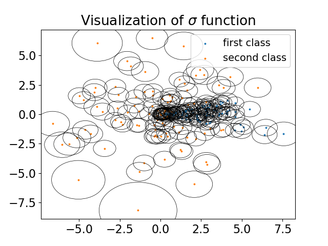
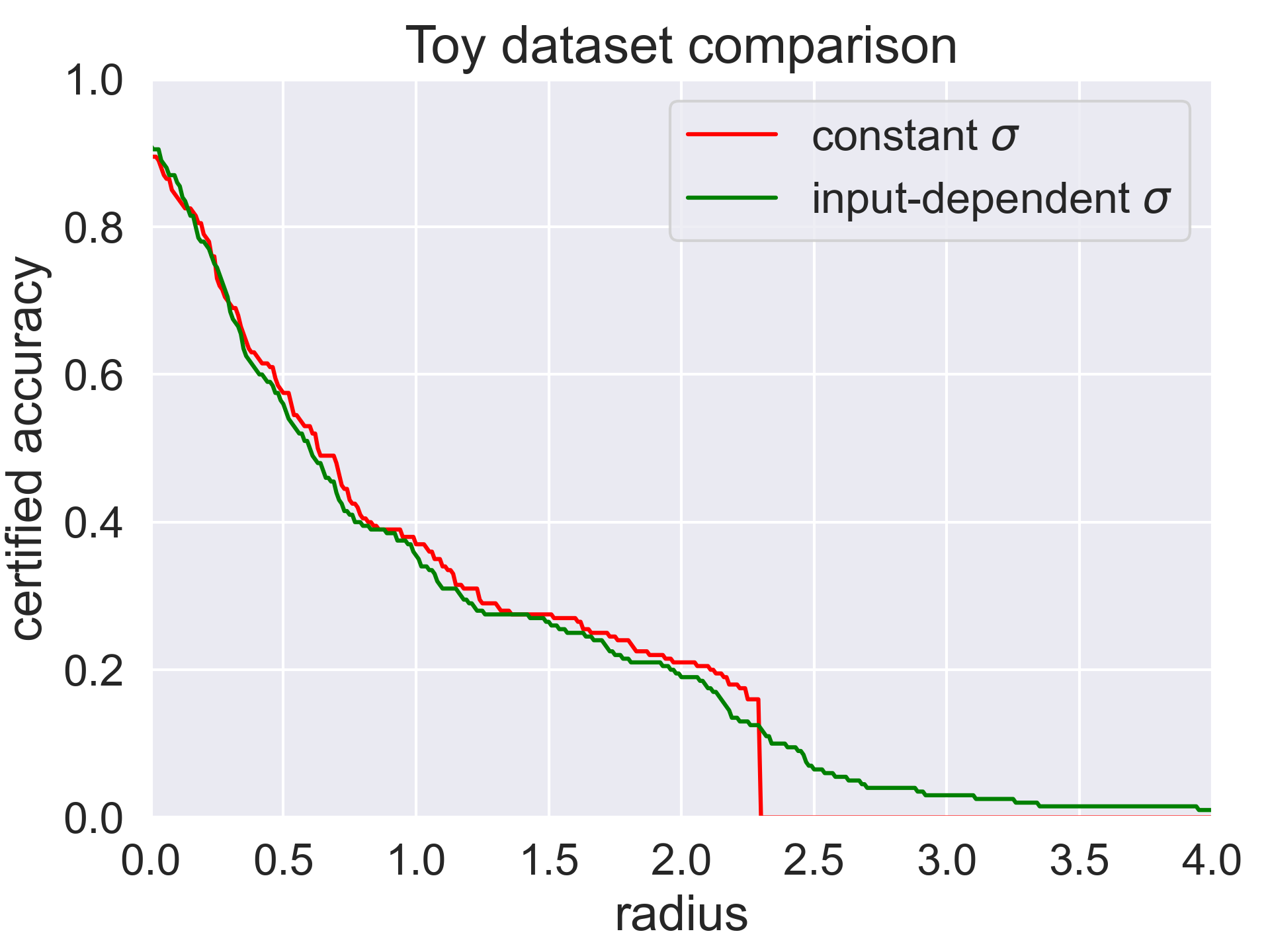
Figure 1: Motivating toy experiment. We use constant $\sigma=0.6$ and input-dependent $\sigma(x)$ equal in average to the constant $\sigma$. Left: Dataset and the variance function depicted as circles with the radius equal to $\sigma(x)$ and centers at the data points. Middle: Zoomed in part of the dataset and decision boundaries of the smoothed classifiers with constant $\sigma$ (red) and input-dependent $\sigma(x)$ (green). Note that we recover a part of the misclassified data points by using a more appropriate smoothing strength close to the decision boundary. Right: Certified accuracy plot. The waterfall effect vanishes since the points far from the decision boundary are certified with a correspondingly large $\sigma(x)$.

The main contributions of this work are fourfold. First, we generalize the methodology of Cohen et al. (2019) for the case of the input-dependent RS (IDRS), obtaining useful and important insights about how to use the Neyman-Pearson lemma in this general case. Second and most importantly, we show that the IDRS suffers from the curse of dimensionality in the sense that the semi-elasticity coefficient $r$ of $\sigma(x)$ (a positive number such that $|\log(\sigma(x_{0}))-\log(\sigma(x_{1}))|\leq r\lVert x_{0}-x_{1}\rVert\hskip 2.84526pt\forall x_{0},x_{1}\in\mathbb{R}^{N}$) in a high-dimensional setting is restricted to be very small. This means, that even if we wanted to vary $\sigma(x)$ significantly with varying $x$, we cannot. The maximal reasonable speed of change of $\sigma(x)$ turns out to be almost too small to handle, especially in high dimensions. Third, in contrast, we also study the conditions on $\sigma(x)$ under which it is applicable in high-dimensional regime and prepare a theoretical framework necessary to build an efficient certification algorithm. We are the first to do so for $\sigma(x)$ functions, which are not locally constant (as in (Wang et al., 2021)). Finally, we provide a concrete design of the $\sigma(x)$ function, test it extensively and compare it to the classical RS on the CIFAR10 and MNIST datasets. We discuss to what extent the method treats the issues mentioned above.

2 IDRS and the Curse of Dimensionality

Let $\mathcal{C}$ be the set of classes, $f:\mathbb{R}^{N}\xrightarrow[]{}\mathcal{C}$ a classifier (referred to as the base classifier), $\sigma:\mathbb{R}^{N}\xrightarrow[]{}\mathbb{R}$ a non-negative function and $\mathcal{P}(\mathcal{C})$ a set of distributions over $\mathcal{C}$. Then we call $G_{f}:\mathbb{R}^{N}\xrightarrow[]{}\mathcal{P}(\mathcal{C})$ the smoothed class probability predictor, if ${G_{f}(x)}_{C}=\mathbb{P}(f(x+\epsilon)=C),$ where $\epsilon\sim\mathcal{N}(0,\sigma(x)^{2}I)$ and $g_{f}:\mathbb{R}^{N}\xrightarrow[]{}\mathcal{C}$ is called smoothed classifier if $g_{f}(x)=\operatorname*{arg\,max}_{C}{G_{f}(x)}_{C}$, for $C\in\mathcal{C}$. We will omit the subscript $f$ in $g_{f}$ often, since it is usually clear from the context to which base classifier the $g$ corresponds. Furthermore, let $A:=g(x)$ refer to the most likely class under the random variable $f(\mathcal{N}(x,\sigma^{2}I))$, and $B$ denote the second most likely class. Define $p_{A}={G_{f}(x)}_{A}$ and $p_{B}={G_{f}(x)}_{B}$ as the respective probabilities. It is important to note that in practice, it is impossible to estimate $p_{A}$ and $p_{B}$ precisely. Instead, $p_{A}$ is estimated as a lower confidence bound (LCB) of the relative occurence of class $A$ in the predictions of $f$ given certain number of Monte-Carlo samples $n$ and a confidence level $\alpha$. The estimate is denoted as $\underline{p_{A}}$. Similarly to Cohen et al. (2019) we use the exact Clopper-Pearson interval for estimation of the LCB. The same applies for $p_{B}$. We work with $l_{2}$-norms denoted as $\lVert x\rVert$. When we speak of certified radius at sample $x_{0}$, we always mean the biggest $R\geq 0$ for which the underlying theory provides the guarantee $g(x_{0})=g(x_{1})\hskip 5.69054pt\forall x_{1}:\lVert x_{0}-x_{1}\rVert\leq R$.

First of all, we summarize the main steps in the derivation of certified radius around $x_{0}$ using any method that relies on the Neyman-Pearson lemma (e.g. by Cohen et al. (2019)).

1. For a potential adversary $x_{1}$ specify the worst-case classifier $f^{*}$, such that $\mathbb{P}(f^{*}(\mathcal{N}(x_{0},\sigma^{2}I))=A)=p_{A}$, while $\mathbb{P}(f^{*}(\mathcal{N}(x_{1},\sigma^{2}I))=B)$ is maximized.

2. Express ${G_{f^{*}}(x_{1})}_{B}=\mathbb{P}(f^{*}(\mathcal{N}(x_{1},\sigma^{2}I))=B)$ as a function depending on $x_{1}$.

3. Determine the conditions on $x_{1}$ (possibly related to $\lVert x_{0}-x_{1}\rVert$) for which this probability is $\leq 0.5$. From these conditions, derive the certified radius.

Cohen et al. (2019) proceeds in this way to obtain a tight certified radius $R=\frac{\sigma}{2}(\Phi^{-1}(\underline{p_{A}})-\Phi^{-1}(\overline{p_{B}}))$. Unfortunately, their result is not directly applicable to the input-dependent case. Constant $\sigma$ simplifies the derivation of $f^{*}$ that turns out to be a linear classifier. This is not the case for non-constant $\sigma(x)$ anymore. Therefore, we generalize the methodology of Cohen et al. (2019). We put $p_{B}=1-p_{A}$ for simplicity (yet it is not necessary to assume this, see Appendix B.5). Let $x_{0}$ be the point to certify, $x_{1}$ the potential adversary point, $\delta=x_{1}-x_{0}$ the shift and $\sigma_{0}=\sigma(x_{0})$, $\sigma_{1}=\sigma(x_{1})$ the standard deviations used in $x_{0}$ and $x_{1}$, respectively. Furthermore, let $q_{i}$ be a density and $\mathbb{P}_{i}$ a probability measure corresponding to $\mathcal{N}(x_{i},\sigma_{i}^{2}I)$, $i\in\{0,1\}$.

Lemma 2.1.

Out of all possible classifiers $f$ such that ${G_{f}(x_{0})}_{B}\leq p_{B}=1-p_{A}$, the one, for which ${G_{f}(x_{0}+\delta)}_{B}$ is maximized predicts class $B$ in a region determined by the likelihood ratio:

$$B=\left\{x\in\mathbb{R}^{N}:\frac{q_{1}(x)}{q_{0}(x)}\geq\frac{1}{r}\right\},$$

where $r$ is fixed, such that $\mathbb{P}_{0}(B)=p_{B}$. Note that we use $B$ to denote both the class and the region of that class.

We use this lemma to compute the decision boundary of the worst-case classifier $f^{*}$.

Theorem 2.2.

If $\sigma_{0}>\sigma_{1}$, then set $B$ is an $N$-dimensional ball with the center at $S_{>}$ and radius $R_{>}:=R_{>}(\sigma_{0},\sigma_{1},\delta,N,r)$, defined in Appendix LABEL:appF:_proofs:

$$S_{>}=x_{0}+\frac{\sigma_{0}^{2}}{\sigma_{0}^{2}-\sigma_{1}^{2}}\delta.$$

If $\sigma_{0}<\sigma_{1}$, then set $B$ is the complement of an $N$-dimensional ball with the center at $S_{<}$ and radius $R_{<}:=R_{<}(\sigma_{0},\sigma_{1},\delta,N,r)$, expressed in Appendix LABEL:appF:_proofs:

$$S_{<}=x_{0}-\frac{\sigma_{0}^{2}}{\sigma_{1}^{2}-\sigma_{0}^{2}}\delta.$$

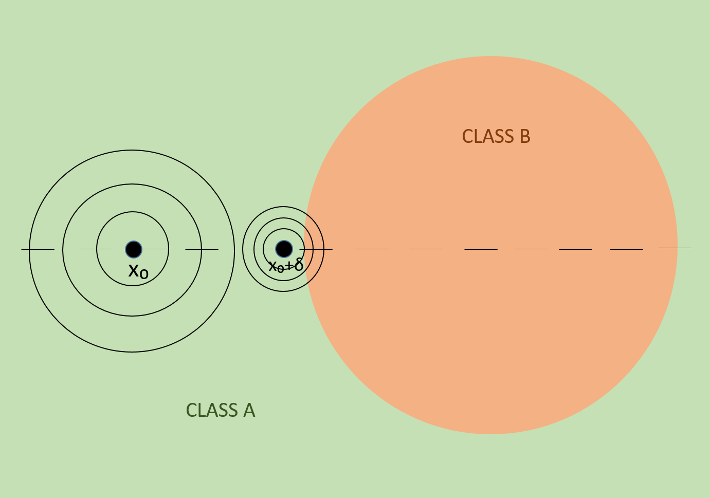
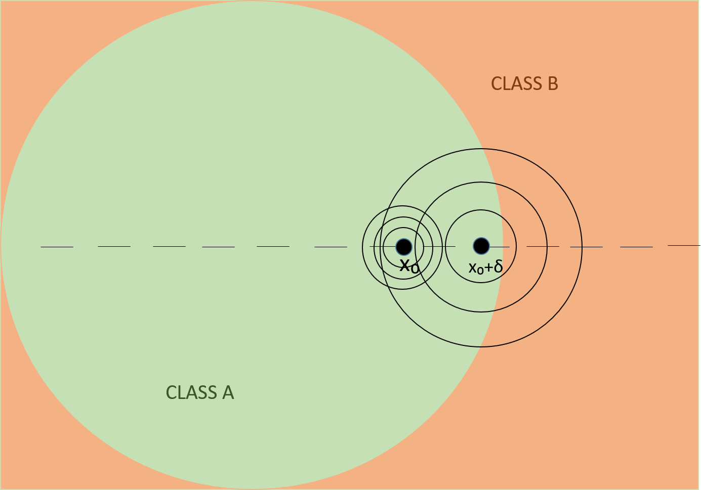
Figure 2: Decision regions of the worst-case classifier $f^{*}$. Left: $\sigma_{0}>\sigma_{1}$ Right: $\sigma_{0}<\sigma_{1}$.

As we depict in Figure 2, both resulting balls are centered on the line connecting $x_{0},x_{1}$. Moreover, the centers of the balls are always further from $x_{0}$, than $x_{1}$ is from $x_{0}$ (even in the case $\sigma_{0}<\sigma_{1}$). In both cases, it depends on $p_{A}$ (since $r$ is fixed such that $\mathbb{P}_{0}(B)=p_{B}$) and the ball can, but might not cover $x_{0}$ and/or $x_{1}$. Note that if $\sigma_{0}=\sigma_{1}$, which can happen even in input-dependent regime, the worst-case classifier is the half-space described by Cohen et al. (2019).

To compute the probability of a ball under an isotropic Gaussian probability measure is more challenging than the probability of a half-space. In fact, there is no closed-form expression for it. However, this probability is connected to the non-central chi-squared distribution (NCCHSQ). More precisely, the probability of an $N$-dimensional ball centered at $z$ with radius $r$ under $\mathcal{N}(0,I)$ can be expressed as a cumulative distribution fucntion (cdf) of NCCHSQ with $N$ degrees of freedom, non-centrality parameter $\lVert z\rVert^{2}$ and argument $r^{2}$. With this knowledge, we can express $\mathbb{P}_{0}(B)$ and $\mathbb{P}_{1}(B)$ in terms of the cdf of NCCHSQ as follows.

Theorem 2.3.

$$\mathbb{P}_{0}(B)=\chi^{2}_{N}\left(\frac{\sigma_{0}^{2}}{(\sigma_{0}^{2}-\sigma_{1}^{2})^{2}}\lVert\delta\rVert^{2},\frac{R_{<,>}^{2}}{\sigma_{0}^{2}}\right),$$

$$\mathbb{P}_{1}(B)=\chi^{2}_{N}\left(\frac{\sigma_{1}^{2}}{(\sigma_{0}^{2}-\sigma_{1}^{2})^{2}}\lVert\delta\rVert^{2},\frac{R_{<,>}^{2}}{\sigma_{1}^{2}}\right),$$

where the sign $<$ or $>$ is chosen according to the inequality between $\sigma_{0}$ and $\sigma_{1}$, and $\chi^{2}_{N}$ is the cdf of NCCHSQ with $N$ degrees of freedom.

Note that both Theorem 2.2 and Theorem 2.3 work well also for $\delta=0$ (see the proofs in Appendix LABEL:appF:_proofs). In this case, we encounter a ball centered at $x_{0}=x_{1}$ and all the cdf functions become cdf functions of central chi-squared.

We expressed the probabilities of the decision region of the worst-case class $B$ using the cdf of NCCHCSQ. Now, how do we do the certification? We start with the certification just for two points, $x_{0}$ for which the certified radius is in question and its potential adversary $x_{1}$. We ask, under which circumstances can $x_{1}$ be certified from the point of view of $x_{0}$. To obtain $\mathbb{P}_{1}(B)$ as a function of $x_{1}$ as in step 2 of the certified radius derivation scheme from page 2, we first need to fix $\mathbb{P}_{1}(B)=1-p_{A}=p_{B}$. Having $x_{0},x_{1}$, $p_{A}$ and $\sigma_{0}>\sigma_{1}$, we obtain such $R$, that $\mathbb{P}_{0}(B)=\chi^{2}_{N}\left(\lVert\delta\rVert^{2}\sigma_{0}^{2}/(\sigma_{0}^{2}-\sigma_{1}^{2})^{2},R^{2}\right)=1-p_{A}=p_{B}$ simply by putting it into the quantile function. This way we get $R^{2}=\chi^{2}_{N,\text{qf}}\left(\lVert\delta\rVert^{2}\sigma_{0}^{2}/(\sigma_{0}^{2}-\sigma_{1}^{2})^{2},1-p_{A}\right)$. In the next step we substitute it directly into $\mathbb{P}_{1}(B)=\chi^{2}_{N}\left(\lVert\delta\rVert^{2}\sigma_{1}^{2}/(\sigma_{0}^{2}-\sigma_{1}^{2})^{2},R^{2}\sigma_{0}^{2}/\sigma_{1}^{2}\right)$. This way, we obtain $\mathbb{P}_{1}(B)$ and can judge, whether $\mathbb{P}_{1}(B)<1/2$ or not. Similar computation can be done if $\sigma_{0}<\sigma_{1}$. Denote $a:=\lVert\delta\rVert$. We express $\mathbb{P}_{1}(B)$ more simply as a function of $a$ for $\sigma_{0}>\sigma_{1}$ as

$$\xi_{>}(a):=\mathbb{P}_{1}(B)=$$

$$\chi^{2}_{N}\left(\frac{\sigma_{1}^{2}}{(\sigma_{0}^{2}-\sigma_{1}^{2})^{2}}a^{2},\frac{\sigma_{0}^{2}}{\sigma_{1}^{2}}\chi^{2}_{N,qf}\left(\frac{\sigma_{0}^{2}}{(\sigma_{0}^{2}-\sigma_{1}^{2})^{2}}a^{2},1-p_{A}\right)\right)$$

and for $\sigma_{0}<\sigma_{1}$ as

$$\xi_{<}(a):=\mathbb{P}_{1}(B)=$$

$$1-\chi^{2}_{N}\left(\frac{\sigma_{1}^{2}}{(\sigma_{1}^{2}-\sigma_{0}^{2})^{2}}a^{2},\frac{\sigma_{0}^{2}}{\sigma_{1}^{2}}\chi^{2}_{N,qf}\left(\frac{\sigma_{0}^{2}}{(\sigma_{1}^{2}-\sigma_{0}^{2})^{2}}a^{2},p_{A}\right)\right)$$

With this in mind, if we have $x_{0},x_{1},p_{A},\sigma_{0},\sigma_{1}$, then we can certify $x_{1}$ w.r.t $x_{0}$ simply by choosing the correct sign ($<,>$), computing $\xi_{<}(\lVert x_{0}-x_{1}\rVert)$ or $\xi_{>}(\lVert x_{0}-x_{1}\rVert)$ and comparing it with $0.5$. The sample plots of these $\xi$ functions can be found in Appendix B.

Now, we are ready to discuss the curse of dimensionality. The problem that arises is that having a high dimension $N$ and $\sigma_{0},\sigma_{1}$ differing a lot from each other, $\xi$ functions are already big at 0, even for considerably small $p_{B}$. For fixed ratio $\sigma_{0}/\sigma_{1}$ and probability $p_{B}$, $\xi(0)$ increases with growing dimension $N$ and soon becomes bigger than 0.5. This, together with monotonicity of the $\xi$ function yields that no $x_{1}$ can be certified w.r.t. $x_{0}$, if $\sigma_{0},\sigma_{1}$ are used. The more dissimilar the $\sigma_{0}$ and $\sigma_{1}$ are, the smaller the dimension $N$ needs to be for this situation to occur. If we want to certify $x_{1}$ in a reasonable distance from $x_{0}$, we need to use similar $\sigma_{0},\sigma_{1}$. This restricts the variability of the $\sigma(x)$ function. We formalize the curse of dimensionality in the following theorems. We discuss more why the curse of dimensionality is present in Appendix B.2.

Theorem 2.4 (curse of dimensionality).

Let $x_{0}$, $x_{1}$, $p_{A}$, $\sigma_{0}$, $\sigma_{1}$ and $N$ be as usual. The following two implications hold:

1. If $\sigma_{0}>\sigma_{1}$ and

   $$\log\left(\frac{\sigma_{1}^{2}}{\sigma_{0}^{2}}\right)+1-\frac{\sigma_{1}^{2}}{\sigma_{0}^{2}}<\frac{2\log(1-p_{A})}{N},$$

   then $x_{1}$ is not certified w.r.t. $x_{0}$.

2. If $\sigma_{0}<\sigma_{1}$ and

   $$\log\left(\frac{\sigma_{1}^{2}}{\sigma_{0}^{2}}\frac{N-1}{N}\right)+1-\frac{\sigma_{1}^{2}}{\sigma_{0}^{2}}\frac{N-1}{N}<\frac{2\log(1-p_{A})}{N},$$

   then $x_{1}$ is not certified w.r.t. $x_{0}$.

Corollary 2.5 (one-sided simpler bound).

Let $x_{0}$, $x_{1}$, $p_{A}$, $\sigma_{0}$, $\sigma_{1}$ and $N$ be as usual and assume now $\sigma_{0}>\sigma_{1}$. Then, if

$$\frac{\sigma_{1}}{\sigma_{0}}<\sqrt{1-2\sqrt{\frac{-\log(1-p_{A})}{N}}},$$

then $x_{1}$ is not certified w.r.t $x_{0}$.

Note that both Theorem 2.4 and Corrolary 2.5 can be adjusted to the case where we have a separate estimate $\overline{p_{B}}$ and do not put $\overline{p_{B}}=1-\underline{p_{A}}$ (see Appendix B.5). We emphasize, that the bounds obtained in Theorem 2.4 are very tight. In other words, if the ratio $\sigma_{1}/\sigma_{0}$ is just slightly bigger than the minimal possible threshold from Theorem 2.4, $\xi_{>}(0)$ becomes smaller than $0.5$ and similarly for $\xi_{<}(0)$. This is because the only two estimates used in the proof of Theorem 2.4 are the estimates on the median, which are very tight and constant with respect to $N$, and the multiplicative Chernoff bound, which is generally considered to be tight too and improves for larger $N$. The tightness is depicted in Figure 3, where we plot the minimal possible threshold $\sigma_{1}/\sigma_{0}$ given by Theorem 2.4 and minimal threshold for which $\xi_{>}(0)<0.5$ as a function of $N$.

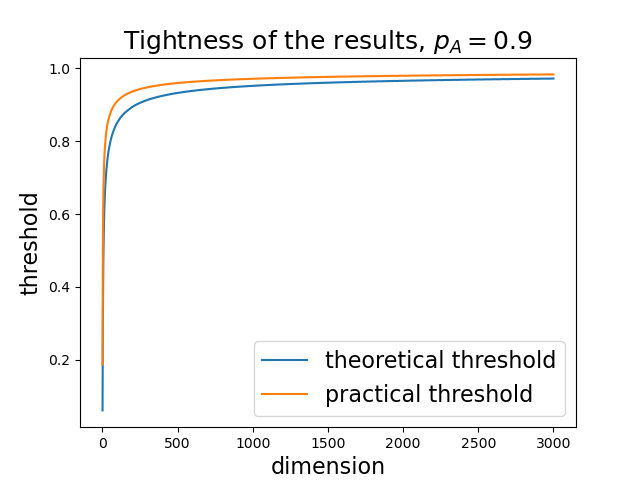
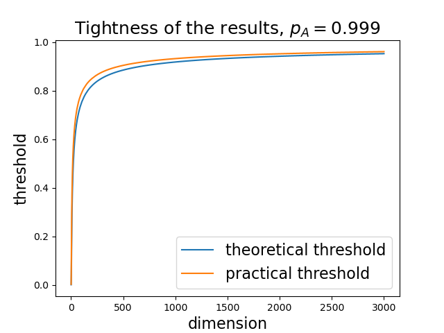
Figure 3: Plots depicting tightness of results of Theorem 2.4. In both figures, the biggest possible threshold of $\sigma_{1}/\sigma_{0}$ for which the condition in Theorem 2.4 is satisfied (theoretical threshold) and the numerically computed threshold for which $\xi_{>}(0)$ exceeds the threshold 0.5 (practical threshold) are depicted. Left: Plot for $p_{A}=0.9$, Right: Plot for $p_{A}=0.999$.

To get a better feeling about the concrete numbers, we provide the theoretical threshold values from Theorem 2.4 in Table 1. If $\sigma_{1}/\sigma_{0}$ is smaller than the threshold, we are not able to certify any pair of $x_{0},x_{1}$ using $\sigma_{0},\sigma_{1}$.

Table 1: Theoretical lower-thresholds for $\sigma_{1}/\sigma_{0}$ for different data dimensions and class $A$ probabilities. The ImageNet spatial size is assumed to be 3x256x256, while CIFAR10 spatial size is 32x32x3 and MNIST spatial size is 28x28x1.

$p_{A}$	$0.9$	$0.99$	$0.999$	$0.99993$
MNIST	0.946	0.924	0.908	0.892
CIFAR10	0.973	0.961	0.953	0.945
ImageNet	0.997	0.995	0.994	0.993

Results from Table 1 are very restrictive. Assume we have a CIFAR10 sample with $\underline{p_{A}}=0.999$. For such a probability, constant $\sigma=0.5$ is more than sufficient to guarantee the certified radius of more than 1. However, in the non-constant regime, to certify $R\geq 1$, we first need to guarantee that no sample within the distance of 1 from $x_{0}$ uses $\sigma_{1}<0.953\sigma_{0}$. To even strengthen this statement, note that one needs to guarantee $\sigma_{1}$ to be even much closer to $\sigma_{0}$ in practice. Why? The results of Theorem 2.4 lower-bound the $\xi$ functions at 0. However, since $\xi$ functions are strictly increasing (as shown in Appendix LABEL:appF:_proofs), one usually needs $\sigma_{0}$ and $\sigma_{1}$ to be much closer to each other to guarantee $\xi(a)$ being smaller than $0.5$ at $a\gg 0$. This not only forces the $\sigma(x)$ function to have really small semi-elasticity but also makes it problematic to define a stochastic $\sigma(x)$. For more, see Appendix B.2.

To fully understand how the curse of dimensionality affects the usage of IDRS, we mention two more significant effects. First, with increasing dimension the average distance between samples tends to grow as $\sqrt{N}$. This enables bigger distance to change $\sigma(x)$. On the other hand, the average level of $\sigma(x)$ (like $\sim 0.12,0.25,\dots$) needs to be adjusted also as $\sqrt{N}$ with increasing dimension. The bigger average level of $\sigma(x)$ we use, the more is the semi-elasticity of $\sigma(x)$ restricted by Theorem 2.4 and Theorem 3.2. All together, these two effects combine in a final trend that for $\sigma_{0}$ and $\sigma_{1}$ being variances used in two random test samples, $|\sigma_{0}/\sigma_{1}-1|$ is restricted to go to 0 as $1/\sqrt{N}.$ For detailed explanation, see Appendix B.4.

3 How to Use IDRS properly

As we discuss above, usage of the IDRS is challenging. How can we obtain valid, mathematically justified certified radiuses? Fix some design $\sigma(x)$. If $\sigma(x)$ is not trivial, to get a certified radius at $x_{0}$, we need to go over all the possible adversaries $x_{1}$ in the neighborhood of $x_{0}$ and compute $\sigma_{1}$ and $\xi_{<,>}(a)$. Then, the certified radius is the infimum over $\lVert x_{0}-x_{1}\rVert$ for all uncertified $x_{1}$ points. Of course, this is a priori infeasible. Fortunately, the $\xi$ functions possess a property that helps to simplify this procedure. For convenience, we extend the notation of $\xi$ such that $\xi(a,\sigma_{1})$ additionally denotes the dependence on the $\sigma_{1}$ value.

Theorem 3.1.

Let $x_{0}$, $x_{1}$, $p_{A}$, $\sigma_{0}$ be as usual and denote $\lVert x_{0}-x_{1}\rVert$ by $R$. Then, the following two statements hold:

1. Let $\sigma_{1}\leq\sigma_{0}$. Then, for all $\sigma_{2}:\sigma_{1}\leq\sigma_{2}\leq\sigma_{0}$, if $\xi_{>}(R,\sigma_{2})>0.5$, then $\xi_{>}(R,\sigma_{1})>0.5$.

2. Let $\sigma_{1}\geq\sigma_{0}$. Then, for all $\sigma_{2}:\sigma_{1}\geq\sigma_{2}\geq\sigma_{0}$, if $\xi_{<}(R,\sigma_{2})>0.5$, then $\xi_{<}(R,\sigma_{1})>0.5$.

Theorem 3.1 serves as a monotonicity property. The main gain is, that for each distance $R$ from $x_{0}$, it is sufficient to consider just two adversaries – the one with the biggest $\sigma_{1}$ (if bigger than $\sigma_{0}$) and the one with the smallest $\sigma_{1}$ (if smaller than $\sigma_{0}$). If we cannot certify some point $x_{1}$ at the distance $R$ from $x_{0}$, then we will for sure not be able to certify at least one of the two adversaries with the most extreme $\sigma_{1}$ values.

This, however, does not suffice for most of the reasonable $\sigma(x)$ designs, since it might be still too hard to determine the two most extreme $\sigma_{1}$ values at some distance from $x_{0}$. Therefore, we assume that $\sigma(x)$ is semi-elastic with coefficient $r$. Then we have a guarantee that $\sigma(x_{0})\exp(-ra)\leq\sigma(x_{1})\leq\sigma(x_{0})\exp(ra)$ holds. Thus, we bound the worst-case extreme $\sigma_{1}$-s for every distance $a$. Using this, we guarantee the following certified radius.

Theorem 3.2.

Let $\sigma(x)$ be an $r$-semi-elastic function and $x_{0}$, $p_{A}$, $N$, $\sigma_{0}$ as usual. Then, the certified radius at $x_{0}$ guaranteed by our method is

$$\text{CR}(x_{0})=\sup\left\{R\geq 0:~{}\begin{matrix}\xi_{>}(R,\sigma_{0}\exp(-rR))<0.5\\ \xi_{<}(R,\sigma_{0}\exp(rR))<0.5\end{matrix}\right\}$$

If the underlying set is empty, which is equivalent to $p_{A}\leq 0.5$ (that might occur in practice, as we use a lower bound $\underline{p_{A}}$ instead of $p_{A}$), we cannot certify any radius.

Note that Theorem 3.2 can be adjusted to the case where we have a separate estimate $\overline{p_{B}}$ and do not put $\overline{p_{B}}=1-\underline{p_{A}}$ (see Appendix B.5). Since the bigger the semi-elasticity constant of $\sigma(x)$ is, the worse certifications we obtain, it is important to estimate the constant tightly. Even with a good estimate of $r$, we still get smaller certified radiuses in comparison with using the $\sigma(x)$ exactly, but that is a prize that is inevitable for the feasibility of the method.

The algorithm is then very easy - we just pick sufficiently dense space of possible radiuses and determine the smallest, for which either $\xi_{>}(R,\sigma_{0}\exp(-rR))$ or $\xi_{<}(R,\sigma_{0}\exp(rR))$ is larger than $0.5$. The only non-trivial part is how to evaluate the $\xi$ functions. For small values of $R$, the $\exp(-rR)$ is very close to 1 and from the definition of $\xi$ functions it is obvious that this results in extremely big inputs to the cdf and quantile function of NCCHSQ. To avoid numerical problems, we employ a simple hack where we assume thresholds for $\sigma_{1}$ such that for $R$ small enough, these thresholds are used instead of $\sigma_{0}\exp(\pm rR))$. Unfortunately, the numerical stability still disables the usage of this method on really high-dimensional datasets like ImageNet. For more details on implementation, see Appendix D.

4 The Design of $\sigma(x)$ and Experiments

The only missing ingredient to finally being able to use IDRS is the $\sigma(x)$ function. As we have seen, this function has to be $r$-semi-elastic for rather small $r$ and ideally deterministic. Yet it should at least roughly fulfill the requirements imposed by the motivation – it should possess big values for points far from the decision boundary of $f$ and rather small for points close to it. Adhering to these restrictions, we use the following function:

$$\sigma(x)=\sigma_{b}\exp\left(r\left(\frac{1}{k}\sum\limits_{x_{i}\in\mathcal{N}_{k}(x)}\lVert x-x_{i}\rVert-m\right)\right)$$ (1)

for $\sigma_{b}$ being a base standard deviation, $r$ the required semi-elasticity, $\{x_{i}\}_{i=1}^{d}$ the training set, $\mathcal{N}_{k}(x)$ the $k$ nearest neighbors of $x$ and $m$ the normalization constant. Intuitively, if a sample is far from all other samples, it will be far from the decision boundary, unless the network overfits to this sample. On the other hand, the dense clusters of samples are more likely to be positioned near the decision boundary, since such clusters have a high leverage on the network’s weights, forcing the decision boundary to adapt well to the geometry of the cluster (for more insight on the relation between the geometry of the data and distance from decision boundary see, for example, Baldock et al. (2021)). To use such a function, however, we first prove that it is indeed $r$-semi-elastic.

Theorem 4.1.

The standard deviation function $\sigma(x)$ defined in equation 1 is $r$-semi-elastic.

We test our IDRS and $\sigma(x)$ function extensively. For both CIFAR10 (Krizhevsky, 2009) and MNIST (LeCun et al., 1999) datasets, we analyze series of different experimental setups, including experiments with an input-dependent train-time Gaussian data augmentation. We present a direct comparison of our method with the constant $\sigma$ method using evaluation strategy from (Cohen et al., 2019) (all other experiments, including ablation studies, and the discussion on the hyperparameter selection are presented in Appendix LABEL:appE:_experiments_and_ablations). Here, we compare (Cohen et al., 2019)’s evaluations for $\sigma=0.12,0.25,0.50$ with our evaluations, setting $\sigma_{b}=\sigma$, $r=0.01,0.02$, $k=20$, $m=5,1.5$ (for CIFAR10 and MNIST, respectively), applied on models trained with Gaussian data augmentation, using constant standard deviation roughly equal to the average test-time $\sigma(x)$ or test-time $\sigma$. For CIFAR10, these levels of train-time standard deviation are $\sigma_{tr}=0.126,0.263,0.53$ and for MNIST $\sigma_{tr}=0.124,0.258,0.517$. In this way, the levels of $\sigma(x)$ we use in the direct comparison are spread from the values roughly equal to (Cohen et al., 2019)’s constant $\sigma$ to higher values. The results are depicted in Figure 4.

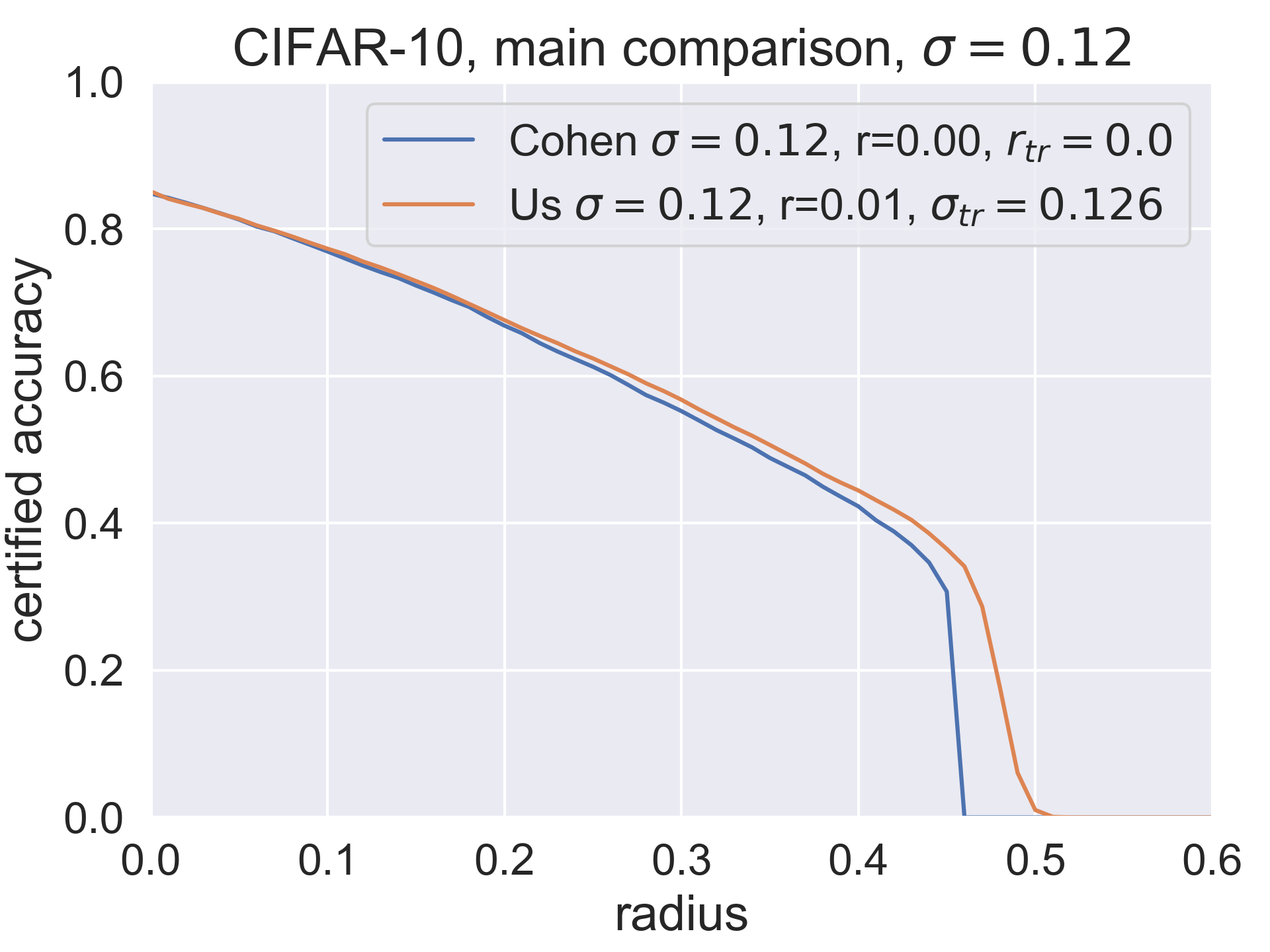
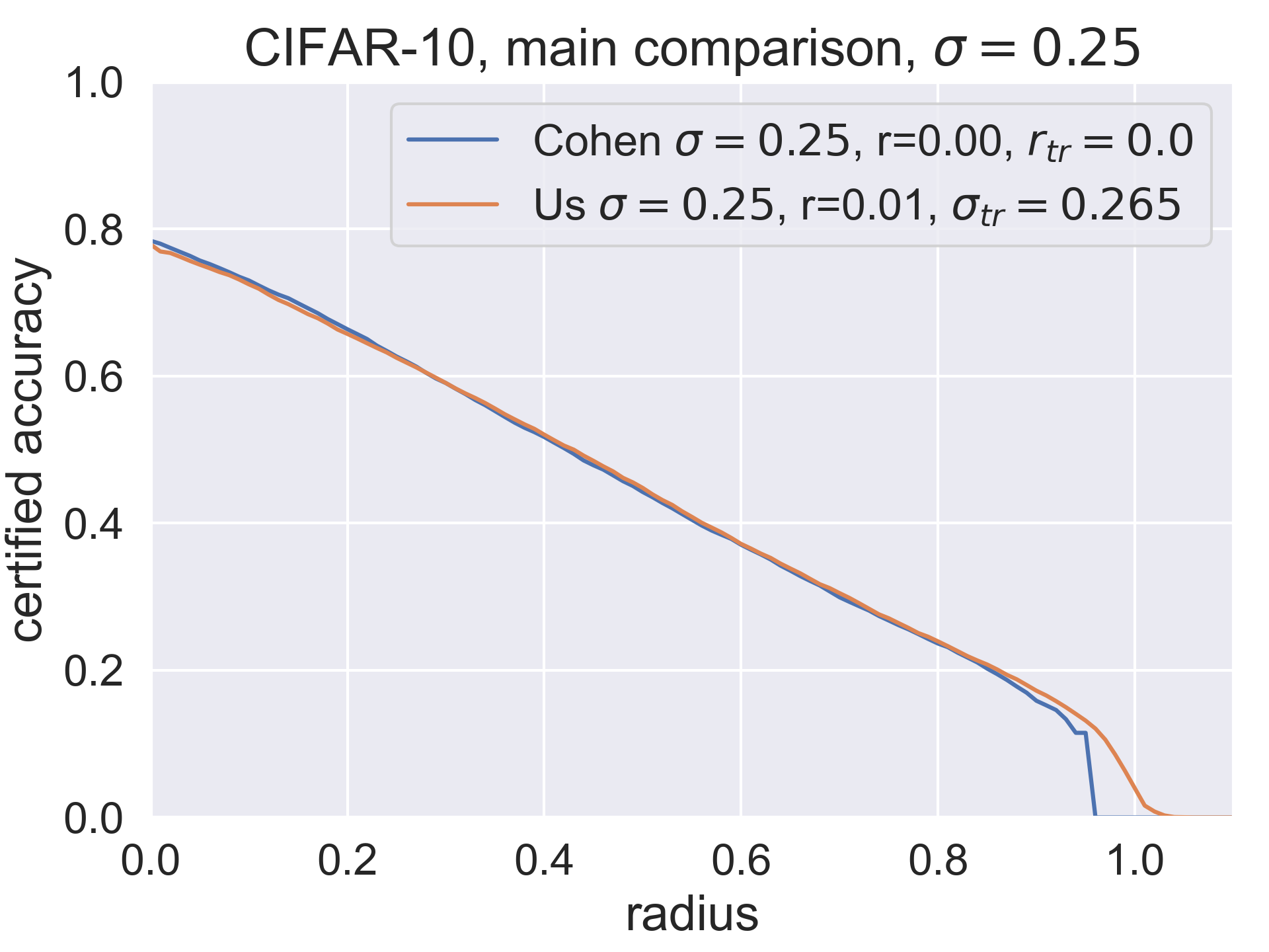
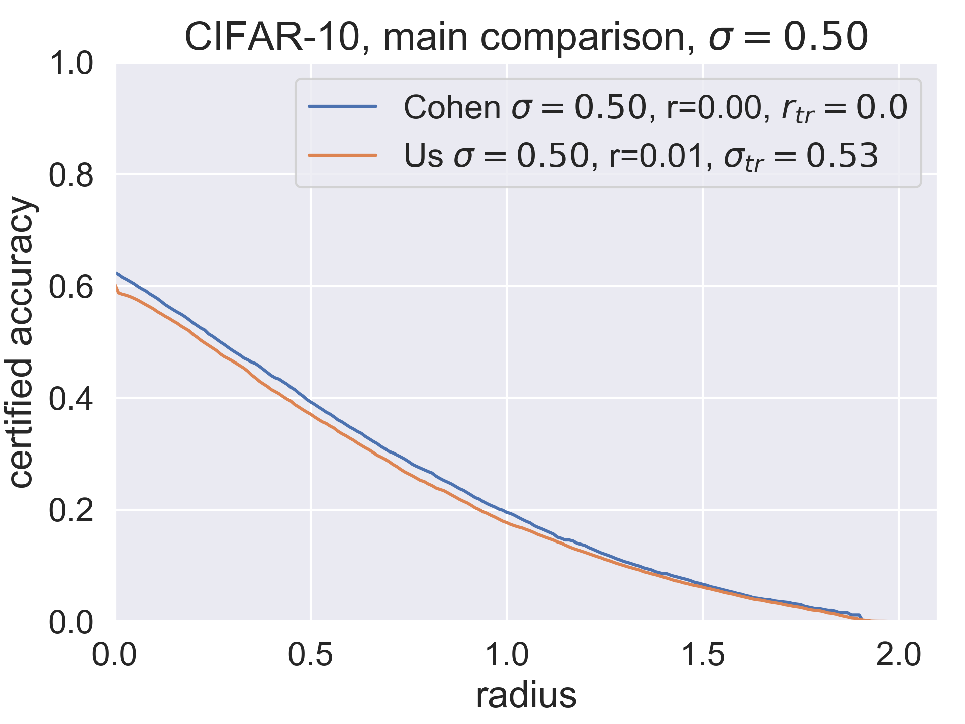
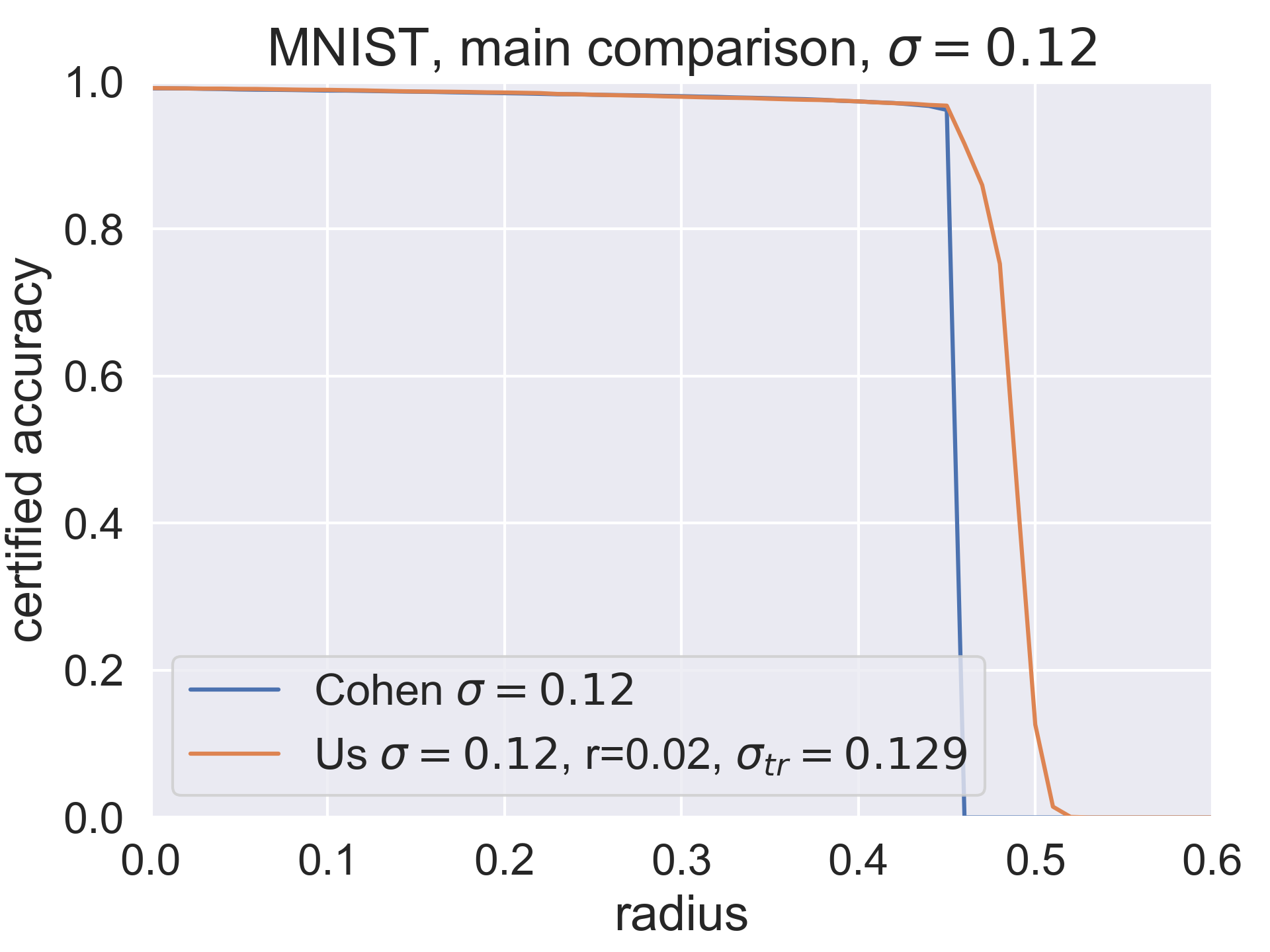
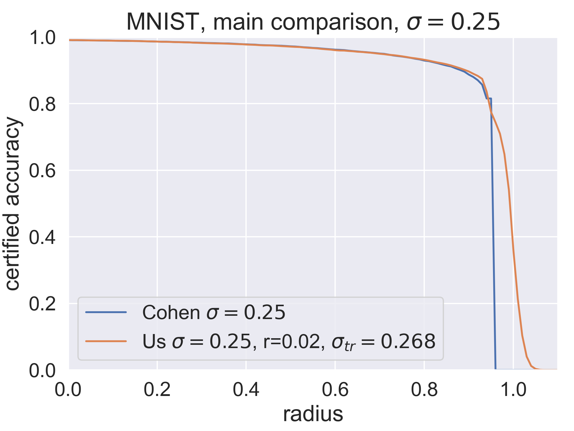
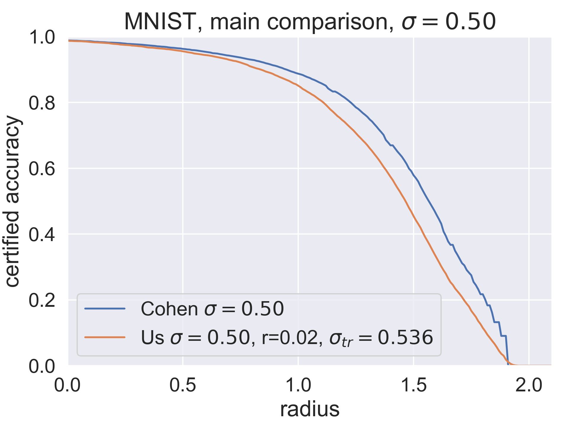
Figure 4: Comparison of certified accuracy plots for Cohen et al. (2019)’s method and our work.

From Figure 4 we see that we outperform the constant $\sigma$ for small levels of $\sigma$, such as $0.12$ or $0.25$. On higher levels of $\sigma$, we are, in general, worse (see explanation in Appendix B.3). The most visible improvement is in mitigation of the truncation of certified accuracy (certified accuracy waterfall). To comment on the other two issues, we provide Tables 2 and 3 with the clean accuracies and class-wise accuracy standard deviations, respectively. These results are the averages of 8 independent runs and in Table 2, the displayed error values are equal to empirical standard deviations.

Table 2: Clean accuracies for both input-dependent and constant $\sigma$ evaluation strategies on CIFAR10 (C) and MNIST (M).

	dataset	$\sigma=0.12$	$\sigma=0.25$	$\sigma=0.50$
$r=0.01,\sigma_{tr}$ increased	C	$0.852\pm 0.002$	$0.780\pm 0.013$	$0.673\pm 0.008$
$r=0.00$	C	$0.851\pm 0.006$	$0.792\pm 0.004$	$0.674\pm 0.018$
$r=0.01,\sigma_{tr}$ increased	M	$0.9912\pm 0.0003$	$0.9910\pm 0.0006$	$0.9881\pm 0.0003$
$r=0.00$	M	$0.9914\pm 0.0004$	$0.9907\pm 0.0004$	$0.9886\pm 0.0005$

Table 3: Class-wise accuracy (i.e. how many points of a certain class are correctly classified divided by the size of this class) standard deviations for both input-dependent and constant $\sigma$ evaluation strategies on CIFAR10 (C) and MNIST (M).

	dataset	$\sigma=0.12$	$\sigma=0.25$	$\sigma=0.50$
$r=0.01,\sigma_{tr}$ increased	C	0.076	0.099	0.120
$r=0.00$	C	0.076	0.097	0.122
$r=0.01,\sigma_{tr}$ increased	M	0.00775	0.00777	0.00930
$r=0.00$	M	0.00751	0.00778	0.00934

From Tables 2 and 3, we draw two conclusions. First, it is not easy to judge about the robustness vs. accuracy trade-off, because the differences in clean accuracies are not statistically significant in any of the experiments (not even for CIFAR10 and $\sigma=0.25$, where the difference is at least pronounced). However, the general trend in Table 2 indicates that the clean accuracies tend to slightly decrease with the increasing rate. The decrease is roughly equivalent to the drop in accuracy for the case when we just use constant $\sigma$ during evaluation with its value set to the average $\sigma(x)$. In that case, the certified radiuses would be also roughly equal in average, but ours would still encounter a less severe certified accuracy drop. Second, the standard deviations of the class-wise accuracies, which serve as a good measure of the impact of the shrinking phenomenon and subsequent fairness, don’t significantly change after applying the non-constant RS.

5 Related Work

Since the vulnerability of deep neural networks against adversarial attacks has been noticed by Szegedy et al. (2013); Biggio et al. (2013), a lot of effort has been put into making neural nets more robust. There are two types of solutions – empirical and certified defenses. While empirical defenses suggest heuristics to make models robust, certified approaches additionally provide a way to compute a mathematically valid robust radius.

One of the most effective empirical defenses, adversarial training (Goodfellow et al., 2014; Kurakin et al., 2016; Madry et al., 2017), is based on a intuitive idea to use adversarial examples for training. Unfortunately, together with adversarial training, other promising empirical defenses were subsequently broken by more sophisticated adversarial methods (for instance by Carlini & Wagner (2017); Athalye & Carlini (2018); Athalye et al. (2018), among others).

Among many certified defenses (Tsuzuku et al., 2018; Anil et al., 2019; Hein & Andriushchenko, 2017; Wong & Kolter, 2018; Raghunathan et al., 2018; Mirman et al., 2018; Weng et al., 2018), one of the most successful yet is RS. While Lecuyer et al. (2019) introduced the method within the context of differential privacy, Li et al. (2019) proceeded via Rényi divergences. Possibly the most prominent work on RS is that of Cohen et al. (2019), where authors fully established RS and proved tight certification guarantees.

Later, a lot of authors further worked with RS. The work of Yang et al. (2020) generalizes the certification provided by Cohen et al. (2019) to certifications with respect to the general $l_{p}$ norms and provide the optimal smoothing distributions for each of the norms. Other works point out different problems or weaknesses of RS such as the curse of dimensionality (Kumar et al., 2020; Hayes, 2020; Wu et al., 2021), robustness vs. accuracy trade-off (Gao et al., 2020) or a shrinking phenomenon (Mohapatra et al., 2020a), which yields serious fairness issues (Mohapatra et al., 2020a).

The work of Mohapatra et al. (2020b) improves RS further by introducing the first-order information about $g$. In this work, authors not only estimate $g(x)$, but also $\nabla g(x)$, making more restrictions on the possible base models $f$ that might have created $g$. Zhai et al. (2020) and Salman et al. (2019) improve the training procedure of $f$ to yield better robustness guarantees of $g$. Salman et al. (2019) directly use adversarial training of the base classifier $f$. Finally, Zhai et al. (2020) introduce the so-called soft smoothing, which enables to compute gradients directly for $g$ and construct a training method, which optimizes directly for the robustness of $g$ via the gradient descent.

To address several issues connected to randomized smoothing, there have already been four works that introduce the usage of IDRS. Wang et al. (2021) divide $\mathbb{R}^{N}$ into several regions $R_{i},i\in\{1,\dots,K\}$ and optimize for $\sigma_{i},i\in\{1,\dots,K\}$ locally, such that $\sigma_{i}$ is a most suitable choice for the region $R_{i}$. Yet this work partially solves some problems of randomized smoothing, it also possesses some practical and philosophical issues (see Appendix C). Alfarra et al. (2020); Eiras et al. (2021); Chen et al. (2021) suggest to optimize for locally optimal $\sigma_{i}$, for each sample $x_{i}$ from the test set. A similar strategy is proposed by these works in the training phase, with the intention of obtaining the base model $f$ that is most suitable for the construction of the smoothed classifier $g$. They demonstrate, that by using this input-dependent approach, one can overcome some of the main problems of randomized smoothing. However, as we demonstrate in Appendix C, their methodology is not valid and therefore their results are not trustworthy. In the latest version of their work, Alfarra et al. (2020) themselves point out this issue and try to fix it by a very similar strategy to the one of Wang et al. (2021). Thus, their work still carries all the problems connected to this method.

6 Conclusions

We show in this work that input-dependent randomized smoothing suffers from the curse of dimensionality. In the high-dimensional regime, the usage of input-dependent $\sigma(x)$ is put under strict constraints. The $\sigma(x)$ function is forced to have very small semi-elasticity. This is in conflict with some recent works, which have used the input-dependent randomized smoothing without mathematical justification and therefore claim invalid results, or results of questionable comparability and practical usability. It seems that input-dependent randomized smoothing has limited potential of improvement over the classical, constant-$\sigma$ RS. Moreover, due to numerical instability, the computation of certified radiuses on high-dimensional datasets like ImageNet remains to be an open challenge.

On the other hand, we prepare a ready-to-use mathematically underlined framework for the usage of the input-dependent RS and show that it works well for small to medium-sized problems. We also show, via extensive experiments, that our concrete design of the $\sigma(x)$ function reasonably mitigates the truncation issue connected to constant-$\sigma$ RS and is capable of mitigating the robustness vs. accuracy one on simpler datasets. The most intriguing and promising direction for the future work lies in the development of new $\sigma(x)$ functions, which could treat the mentioned issues even more efficiently.

This improvement is necessary to make IDRS able to significantly beat constant smoothing, as it happens in our toy example in Appendix A. The difference between CIFAR10 and MNIST and the toy dataset is that $\sigma(x)$ from equation 1 is well-suited for the toy dataset’s geometry, but not to the same extent for the geometry of images. One possible reason is that this $\sigma(x)$ does not correspond to the distances from the decision boundary across the entire dataset, because the euclidean distances between images do not align with the “distances in images’ content”. We believe, however, that improvements in $\sigma(x)$ design are possible and we leave the investigation in this matter as an open and attractive research question. One way to go is to define a metric on the input space that would better reflect the geometry of images and convolutional neural networks.

Appendix A The Issues of Constant $\sigma$ Smoothing

A.1 Toy Example

To better demonstrate our ideas, we prepared a two-dimensional simple toy dataset. This dataset can be seen in Figure 5. The dataset is generated in polar coordinates, having uniform angle and the distance distributed as a square root of suitable chi-square distribution. The classes are positioned in a circle sectors, one in a sector with a very sharp angle. The number of training samples is 500 for each class, number of test samples is 100 for each class (except demonstrative figures, where we increased it to 300). The model that was trained on this dataset was a simple fully connected three-layer neural network with ReLU activations and a maximal width of 20.

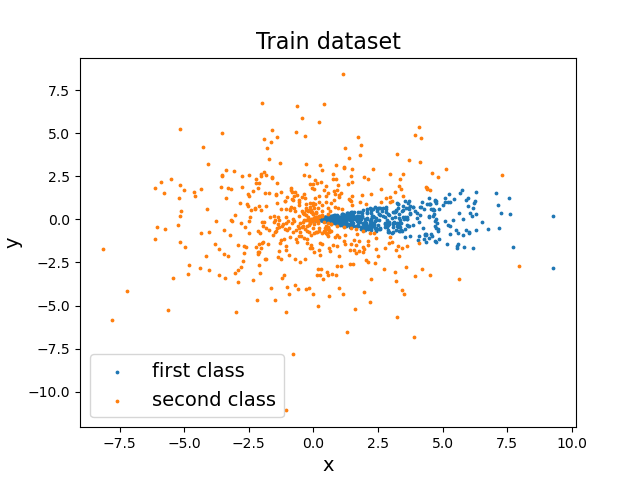
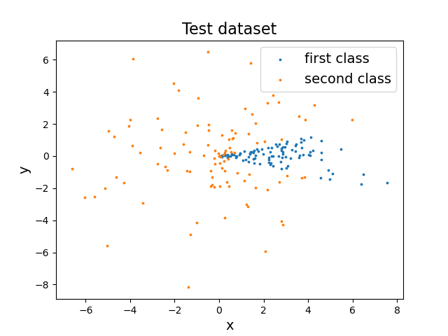
Figure 5: The toy dataset.

A.2 Undercertification Caused by the Use of Lower Confidence Bounds

As we mention in Section 1, one can not usually obtain exact values of $p_{A}$ and $p_{B}$. However, it is obvious, that for vast majority of evaluated samples, $\underline{p_{A}}<p_{A}$ and $\overline{p_{B}}>p_{B}$. Given the nature of our certified radius, it follows that $\underline{R}<R$, where $\underline{R}$ denotes the certified radius coming from the certification procedure with $\underline{p_{A}}$ and $\overline{p_{B}}$, while $R$ here stands for the certified radius corresponding to true values $p_{A},p_{B}$.

It is, therefore, clear, that we face a certain level of under-certification. But how serious under-certification it is? Assume the case with a linear base classifier. Imagine, that we move the point $x$ further and further away from the decision boundary. Therefore, $p_{A}\xrightarrow[]{}1$. At some point, the probability will be so large, that with high probability, all $n$ samplings in our evaluation of $\underline{p_{A}}$ will be classified as $A$, obtaining $\hat{p}_{A}=1$ - the empirical probability. The lower confidence bound $\underline{p_{A}}$ is therefore bounded by having $\hat{p}_{A}=1$. Thus, from some point, the certification will yield the same $\underline{p_{A}}$ regardless of the true value of $p_{A}$. So in practice, we have an upper bound on the certified radius $R$ in the case of the linear boundary. In Figure 7 (left), we see the truncation effect. Using $\sigma=1$, from a distance of roughly 4, we can no longer achieve a better certified radius, despite its theoretical value equals the distance. Similarly, if we fix a distance of $x$ from decision boundary and vary $\sigma$, for very small values of $\sigma$, the value of $\Phi^{-1}(\underline{p_{A}})$ will no longer increase, but the values of $\sigma$ will pull $R$ towards zero. This behaviour is depicted in Figure 7 (right).

We can also look at it differently - what is the ratio between $\Phi^{-1}(p_{A})$ and $\Phi^{-1}(\underline{p_{A}})$ for different values of $p_{A}$? Since $\underline{R}=\sigma\Phi^{-1}(\underline{p_{A}})$ and $R=\sigma\Phi^{-1}(p_{A})$, the ratio represents the “undercertification rate”. In Figure 6 we plot $\frac{\Phi^{-1}(\underline{p_{A}})}{\Phi^{-1}(p_{A})}$ as a function of $p_{A}$ for two different ranges of values. The situation is worst for very small and very big values of $p_{A}$. In the case of very big values, this can be explained due to extreme nature of $\Phi^{-1}$. For small values of $p_{A}$, it can be explained as a consequence of a fact, that even small difference between $p_{A}$ and $\underline{p_{A}}$ will yield big ratio between $\Phi^{-1}(p_{A})$ and $\Phi^{-1}(\underline{p_{A}})$ due to the fact, that these values are close to 0.

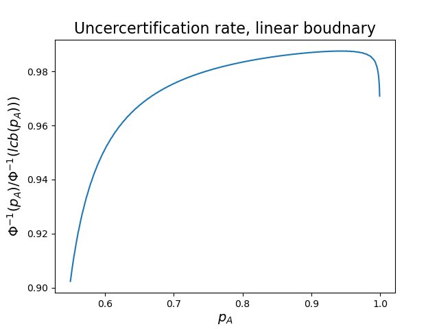
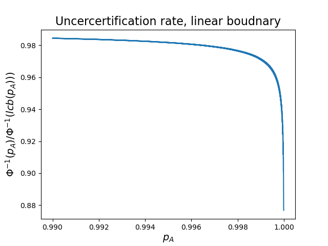
Figure 6: The ratio between certified radius if using lower confidence bounds and if using exact values for the case of linear boundary.

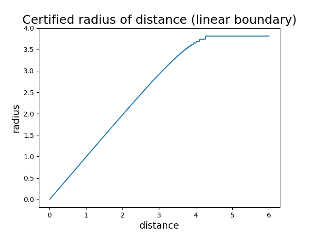
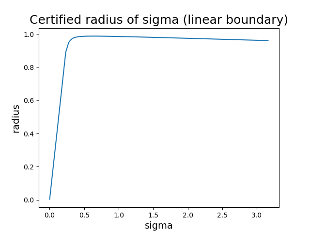
Figure 7: Left: Certified radius as a function of distance in linear boundary case. The truncation is due to the use of lower confidence bounds. The parameters are $n=100000,\alpha=0.001,\sigma=1$. Right: Certified radius for a point $x$ at fixed distance 1 from linear boundary as a function of used $\sigma$. The undercertification follows from usage of lower confidence bounds.

If we look at the left plot on Figure 8 we see, that the certified accuracy plots also possess the truncations. Above some radius, no sample is certified anymore. The problem is obviously more serious for small values of $\sigma$. On the right plot of Figure 8, we see, that samples far from the decision boundary are obviously under-certified. We can also see, that certified radiuses remain constant, even though in reality they would increase with increasing distance from the decision boundary.

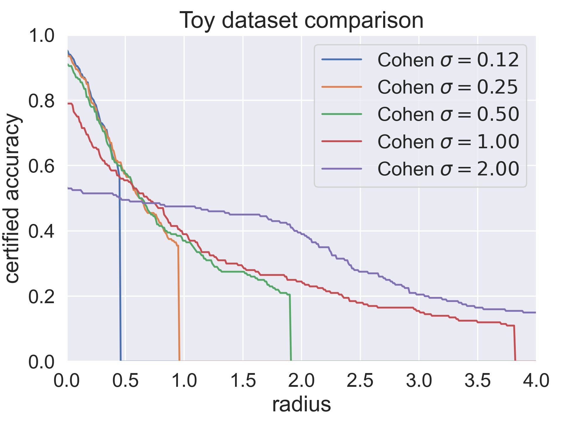
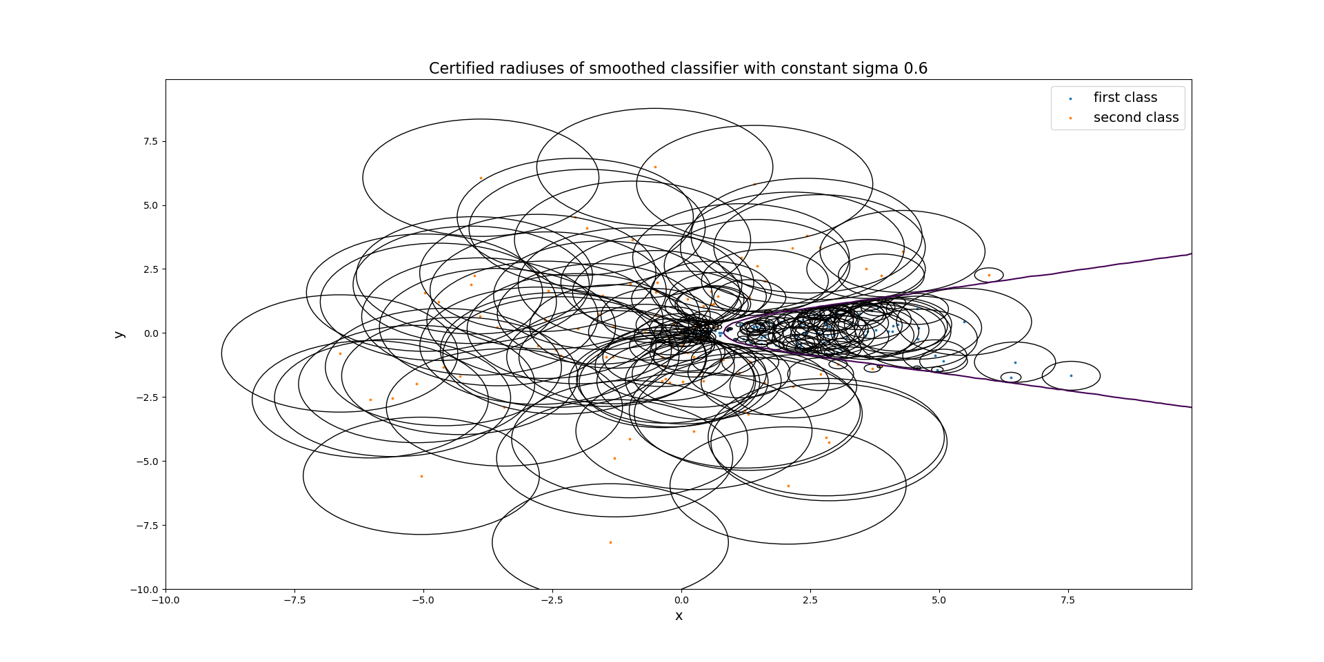
Figure 8: Results of certification on toy dataset. Left: Certified accuracy for different levels of $\sigma$. Right: Certified radiuses and decision boundary of $g$ visualized directly on test set.

All the observations so far motivate us to use rather large values of $\sigma$ in order to avoid the truncation problem. However, as we will see in the next sections, using a large $\sigma$ carries a different, yet equally serious burden.

A.3 Robustness vs. Accuracy Trade-off

As we demonstrate in the previous subsection, it is be useful to use large values of $\sigma$ to prevent the under-certification. But does it come without a prize? If we have a closer look at Figure 8 (right), we might notice, that the accuracy on the threshold $0$, i.e. “clean accuracy”, decreases as $\sigma$ increases. This effect has been noticed in the literature (Cohen et al., 2019; Gao et al., 2020; Mohapatra et al., 2020a) and is called robustness vs. accuracy tradeoff.

There are several reasons, why this problem occurs. Generally, changing $\sigma$ changes the decision boundary of $g$ and we might assume, that due to the high complexity of the boundary of $f$, the decision boundary of $g$ becomes smoother. If $\sigma$ is too large, however, the decision boundary will be so smooth, that it might lose some amount of the base classifier’s expressivity. Another reason for the accuracy drop is also the increase in the number of samples, for which the evaluation is abstained. This is because using big values of $\sigma$ makes more classes “within the reach of our distribution”, making the $p_{A}$ and $\underline{p_{A}}$ small. If $\underline{p_{A}}<0.5$ and we do not estimate $p_{B}$ but set $\overline{p}_{B}=1-\underline{p_{A}}$, then we are not able to classify the sample as class $A$, yet we cannot classify it as a different class either, which forces us to abstain. To demonstrate these results, we computed not only the clean accuracies of (Cohen et al., 2019) evaluations but also the abstention rates. Results are depicted in the Table 4.

	Accuracy	Abstention rate	Misclassification rate
$\sigma=0.12$	0.814	0.038	0.148
$\sigma=0.25$	0.748	0.086	0.166
$\sigma=0.50$	0.652	0.166	0.182
$\sigma=1.00$	0.472	0.29	0.238

Table 4: Accuracies, rates of abstentions and misclassification rates of (Cohen et al., 2019) evaluation for different levels of $\sigma$.

From the table, it is obvious, that the abstention rate is possibly even bigger cause of accuracy drop than the “clean misclassification”. This problem can be partially solved if one estimated $\overline{p_{B}}$ together with $\underline{p_{A}}$ too. In this way, using big $\sigma$ yields generally small estimated class probabilities, but since $p_{A}\geq p_{B}$, the problematic $\overline{p_{B}}\geq\underline{p_{A}}$ occur just very rarely. Another option is to increase the number of Monte-Carlo samplings for the classification decision, what is almost for free.

Yet another reason for the decrease in the accuracy is the so-called shrinking phenomenon, which we will discuss in the next subsection.

In contrast with the truncation effect, the robustness vs. accuracy trade-off motivates the usage of smaller values of $\sigma$ in order to prevent the accuracy loss, which is definitely a very serious issue.

A.4 Shrinking Phenomenon

How exactly does the decision boundary of $g$ change, as we change the $\sigma$? For instance, if $f$ is a linear classifier, then the boundary does not change at all. To answer this question, we employ the following experiment: For our toy base classifier $f$ on our toy dataset, we increase $\sigma$ and plot the heatmap of $f,g$, together with its decision boundary. This experiment is depicted on Figure 9. As we see from the plots, increasing $\sigma$ causes several effects. First of all, the heatmap becomes more and more blurred, what proves, that stronger smoothing implies stronger smoothness.

Second, crucial, effect is that the bigger the $\sigma$, the smaller the decision boundary of a submissive class is. The shrinkage becomes pronounced from $\sigma=1$. Already for $\sigma=4$, there is hardly any decision boundary anymore. Generally, as $\sigma\xrightarrow[]{}\infty$, $g$ will predict the class with the biggest volume in the input space (in the case of bounded input space, like in image domain, this is very well defined). For extreme values of sigma, the $p_{A}$ will practically just be the ratio between the volume of $A$ and the actual volume of the input space (for bounded input spaces).

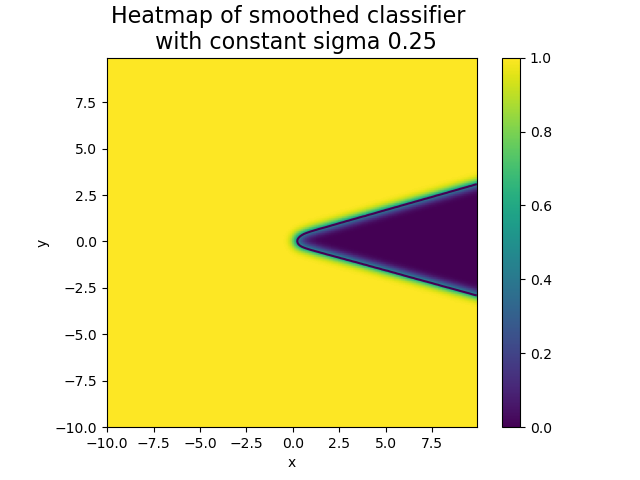
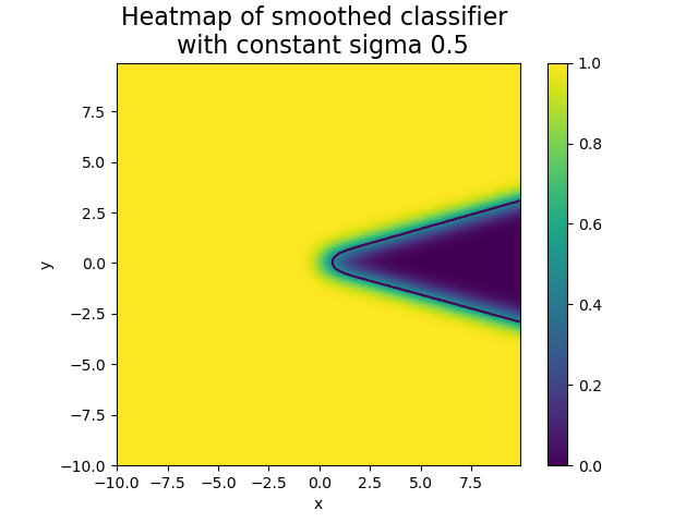
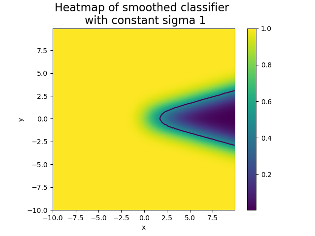
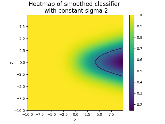
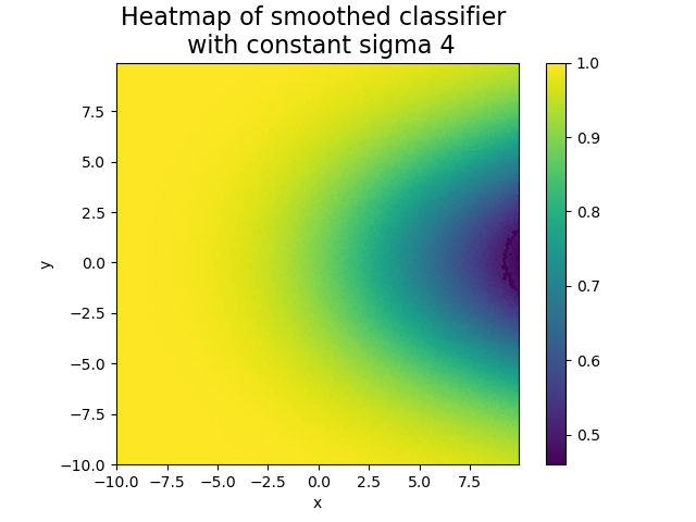
Figure 9: Heatmaps and decision boudnary of base classifier (top left) and the smoothed classifier for increasing levels of $\sigma$. As $\sigma$ increases, the classifier is more smooth and the decision boundary recedes.

Following from these results, but also from basic intuition, it seems, that an undesired effect becomes present as $\sigma$ increases - the bounded/convex regions become to shrink, like in Figure 9, while the unbounded/big/anti-convex regions expand. This is called shrinking phenomenon. (Mohapatra et al., 2020a) investigate this effect rather closely. They define the shrinkage and vanishing of regions formally and prove rigorously, that if $\sigma\xrightarrow[]{}\infty$, bounded regions, or semi-bounded regions (see (Mohapatra et al., 2020a)) will eventually vanish. We formulate the main result in this direction.

Theorem A.1.

Let us have $K$ the number of classes and the dimension $N$. Assume, that we have some bounded decision region $\mathcal{D}$ for a specific class roughly centered around 0. Further assume, that this is the only region where the class is classified. Let $R$ be a smallest radius such that $\mathcal{D}\subset B_{R}(0)$. Then, this decision region will vanish at most for $\sigma\geq\frac{R\sqrt{K}}{\sqrt{N}}$.

Proof.

The idea of the proof is not very hard. First, the authors prove, that the smoothed region will be a subset of the smoothed $B_{R}(0)$. Then, they upper-bound the vanishing threshold of such a ball in two steps. First, they show, that if 0 is not classified as the class, then no other point will be (this is quite an intuitive geometrical statement. The $B_{R}(0)$ has the biggest probability under $\mathcal{N}(x,\sigma^{2}I)$ if $x\equiv 0$). Second, they upper-bound the threshold for $\sigma$, under which $B_{R}(0)$ will have probability below $\frac{1}{K}$ (since they use slightly different setting as (Cohen et al., 2019)) for the $\mathcal{N}(x,\sigma^{2}I)$. Using some insights about incomplete gamma function, which is known to be also the cdf of central chi-square distribution, and some other integration tricks, they obtain the resulting bound. ∎

Besides Theorem A.1, authors also claim many other statements abound shrinking, including shrinking of semi-bounded regions. Moreover, they also conduct experiments on CIFAR10 and ImageNet to support their theoretical findings. They also point out serious fairness issue that comes out as a consequence of the shrinkage phenomenon. For increasing levels of $\sigma$, they measure the class-wise clean accuracy of the smoothed classifier. If $f$ is trained with Gaussian data augmentation (what is known to be a good practice in randomized smoothing), using $\sigma=0.12$, the worst class cat has test accuracy of 67%, while the best class automobile attains the accuracy of 92%. The figures, however, change drastically, if we use $\sigma=1$ instead. In this case, the worst predicted class cat has accuracy of poor 22%, while ship has reasonable accuracy 68%. As authors claim, this is a consequence of the fact that samples of cat are situated more in bounded, convex regions, that suffer from shrinking, while samples of ship are mostly placed in expanded regions of anti-convex shape that will expand as the $\sigma$ grows. In addition, the authors also show, that the Gaussian data augmentation or adversarial training will reduce the shrinking phenomenon just partially and for moderate and high values of $\sigma$, this effect will be present anyway.

We must emphasize, that this is a serious fairness issue, that has to be treated before randomized smoothing can be fully used in practice. For instance, if we trained a neural network to classify humans into several categories, fairness of classification is inevitable and the neural network cannot be used until this issue is solved.

Similarly as the robustness vs. accuracy trade-off, this issue also motivates to use rather smaller values of $\sigma$. We see, that it is not possible to address all three problems consistently because they disagree on whether to use smaller, or bigger values of $\sigma$.

A.5 Experiments on High-dimensional toy Dataset

In this subsection, we present the results of our motivational experiment on a synthetic dataset. Before reading this section, please read our main text, because we will use the necessary notation of the paper.

The dataset we evaluated our method on is a generalization of the dataset visualized on Figure 1. The data points from one class lie in a cone of small angle and the points are generated such that the density is higher near the vertex of the cone (which is put in origin). Points from other class are generated from a spherically symmetrical distribution (where points sampled into the cone are excluded) with density again highest in the center (note, that the density peak is more pronounced than in the case of normal distribution, where the density around the center resembles uniform distribution). This dataset is chosen so that the $\sigma(x)$ function designed in Equation 1 well corresponds to the geometry of the decision boundary. Moreover it is chosen so that the conic decision region will shrink rather fast with increasing $\sigma$. The motivation of this example is to show that if the $\sigma(x)$ function is well-designed, our IDRS can outperform the constant RS considerably.

The setup of our experiment is as follows: We evaluate dimensions $N=2,6,18,60,180,400$. The $\sigma$ used for constant smoothing is $\sigma=0.5,0.5,1.0,1.0,2.0,2.0$ respectively. The $\sigma_{b}$ used is $0.4,0.5$ for $N=2$, $0.4$ for $N=6$, $0.8$ for $N=18$, $0.8,1.0$ for $N=60$, $1.9$ for $N=180$ and $1.95$ for $N=400$. The rates are $r=0.2,0.1,0.05,0.03,0.01,0.005$ respectively. The training was executed without data augmentation (because samples from different classes are very close to each other). Moreover, we have set maximal $\sigma(x)$ threshold for numerical purposes, because some samples were outliers and were way too far from other samples (and if the $\sigma(x)$ is way too big, the method encounteres numerical problems). In this case we set $\sigma(x)\leq 5\sigma_{b}$, but we are aware that also much bigger thresholds would have been possible. We present our comparisons in Figure 10 and Table 5.

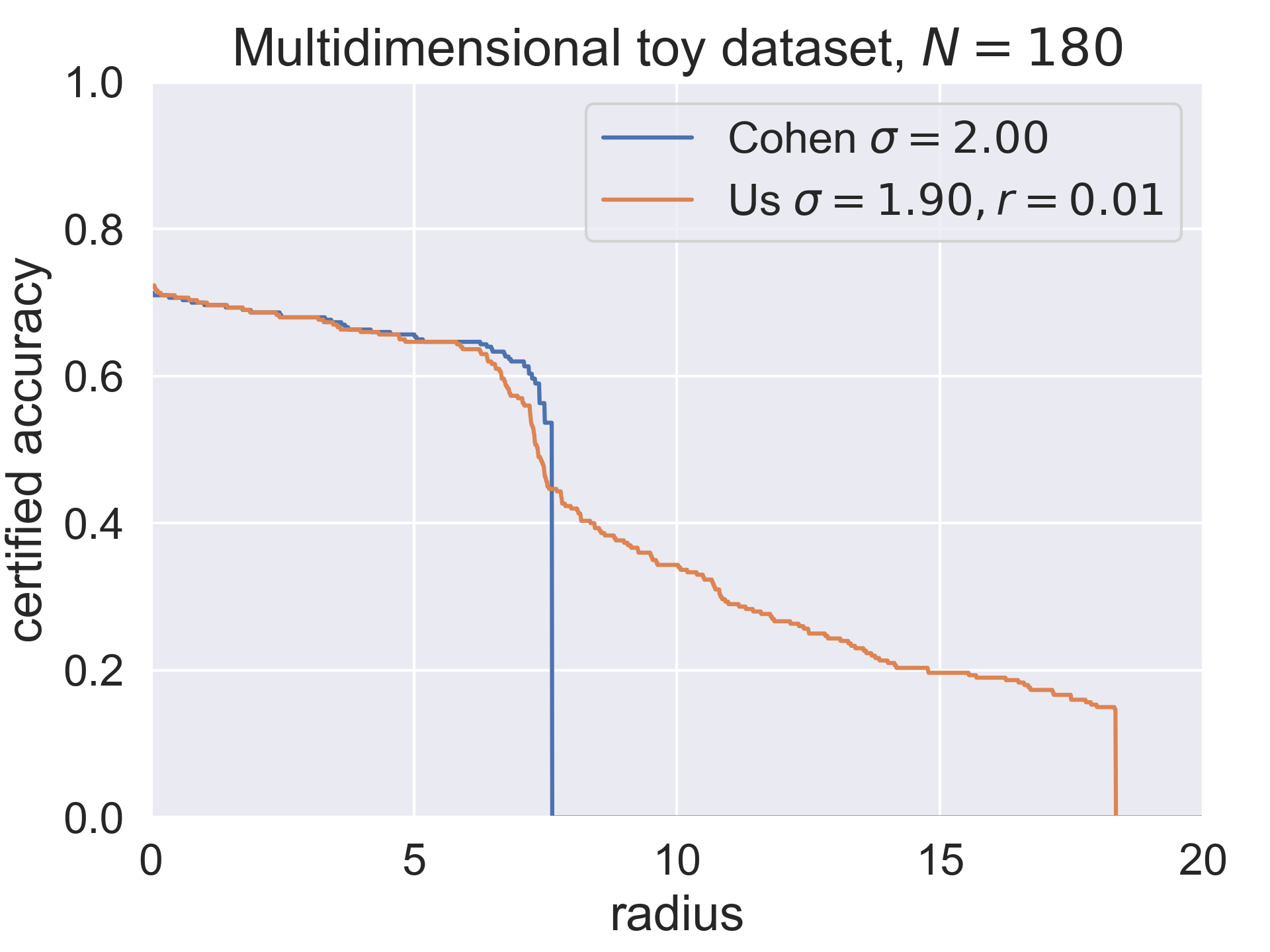
Figure 10: Certified accuracy plots of our multidimensional toy experiments.

Dimension	$\sigma$ ($\sigma_{b}$)	$r$	Accuracy
2	0.5	-	0.943
2	0.4	0.2	0.96
2	0.5	0.2	0.943
6	0.5	-	0.946
6	0.4	0.1	0.963
18	1.0	-	0.86
18	0.8	0.05	0.886
60	1.0	-	0.83
60	0.8	0.03	0.85
60	1.0	0.03	0.83
180	2.0	-	0.713
180	1.9	0.01	0.726
400	2.0	-	0.623
400	1.95	0.005	0.623

Table 5: Clean accuracies of different evaluations of our toy experiment.

From both the Figure 10 an Table 5 it is clear that the IDRS can outperform the constant $\sigma$ RS considerably, if we use really suitable $\sigma(x)$ function. We manage to improve significantly the certified radiuses without losing a single correct classification. On the other hand, in cases where $\sigma_{b}<\sigma$, we outperform constant $\sigma$ both in clean accuracy and in certified radiuses. This example is synthetic and designed in our favour. The main message is not how perfect our design of $\sigma(x)$ is, but the fact, that if $\sigma(x)$ is designed well, the IDRS can bring real advantages, even in moderate dimensions.

Appendix B More on Theory

B.1 Generalization of Results by Li et al. (2019)

In our main text, we mostly focus on the generalization of the methods from (Cohen et al., 2019). This is because these methods yield tight radiuses and because the application of Neyman-Pearson lemma is beautiful. However, the methodology from (Li et al., 2019) can also be generalized for the input-dependent RS. To be able to do it, we need some auxiliary statements about the Rényi divergence.

Lemma B.1.

The Rényi divergence between two one-dimensional normal distributions is as follows:

$$D_{\alpha}(\mathcal{N}(\mu_{1},\sigma_{1}^{2})||\mathcal{N}(\mu_{0},\sigma_{0}^{2}))=\frac{\alpha(\mu_{1}-\mu_{2})^{2}}{2\sigma_{\alpha}^{2}}+\frac{1}{1-\alpha}\log\left(\frac{\sigma_{\alpha}}{\sigma_{1}^{1-\alpha}\sigma_{0}^{\alpha}}\right),$$

provided, that $\sigma_{\alpha}^{2}:=(1-\alpha)\sigma_{1}^{2}+\alpha\sigma_{0}^{2}\geq 0$.

Proof.

See (Van Erven & Harremos, 2014). ∎

Note, that this proposition induces some assumptions on how $\sigma_{0},\sigma_{1},\alpha$ should be related. If $\sigma_{0}>\sigma_{1}$, then the required inequality holds for any $1\neq\alpha>0$. If $\sigma_{0}<\sigma_{1}$, then $\alpha$ is restricted and we need to keep that in mind.

Lemma B.2.

Assume, we have some one-dimensional distributions $\mathcal{P}_{1},\mathcal{P}_{1},\dots,\mathcal{P}_{N}$ and $\mathcal{Q}_{1},\mathcal{Q}_{2},\dots,\mathcal{Q}_{N}$ defined on common space for pairs with the same index. Then, assuming product space with product $\sigma$-algebra, we have the following identity:

$$D_{\alpha}(\mathcal{P}_{1}\times\mathcal{P}_{2}\times\dots\times\mathcal{P}_{N}||\mathcal{Q}_{1}\times\mathcal{Q}_{2}\times\dots\times\mathcal{Q}_{N})=\sum_{i=1}^{N}D_{\alpha}(\mathcal{P}_{i}||\mathcal{Q}_{i}).$$

Proof.

See (Van Erven & Harremos, 2014). ∎

Using these two propositions, we are now able to derive a formula for Rényi divergence between two multivariate isotropic normal distributions:

Lemma B.3.

$$D_{\alpha}(\mathcal{N}(x_{1},\sigma_{1}^{2}I)||\mathcal{N}(x_{0},\sigma_{0}^{2}I))=\frac{\alpha\lVert x_{0}-x_{1}\rVert^{2}}{2\sigma_{1}^{2}+2\alpha(\sigma_{0}^{2}-\sigma_{1}^{1})}+N\frac{\log\left(\frac{\sigma_{\alpha}}{\sigma_{1}}\right)}{1-\alpha}-N\frac{\alpha}{1-\alpha}\log\left(\frac{\sigma_{0}}{\sigma_{1}}\right).$$

Proof.

Imporant property that is needed here is, that isotropic gaussian distributions factorize to one-dimensinal independent marignals. In other words:

$$\mathcal{N}(x_{1},\sigma_{1}^{2}I)=\mathcal{N}(x_{11},\sigma_{1}^{2})\times\mathcal{N}(x_{12},\sigma_{1}^{2})\times\dots\times\mathcal{N}(x_{1N},\sigma_{1}^{2}),$$

and analogically for $x_{0}$. Therefore, using Lemma B.2 we see:

$$D_{\alpha}(\mathcal{N}(x_{1},\sigma_{1}^{2}I)||\mathcal{N}(x_{0},\sigma_{0}^{2}I))=\sum_{i=1}^{N}D_{\alpha}(\mathcal{N}(x_{1i},\sigma_{1}^{2})||\mathcal{N}(x_{0i},\sigma_{0}^{2})).$$

Now, it suffices to plug in the formula from Proposition B.1 to obtain the required result:

$$D_{\alpha}(\mathcal{N}(x_{1i},\sigma_{1}^{2}I)||\mathcal{N}(x_{0i},\sigma_{0}^{2}I)) =\frac{\alpha(x_{1i}-x_{2i})^{2}}{2\sigma_{\alpha}^{2}}+\frac{1}{1-\alpha}\log\left(\frac{\sigma_{\alpha}}{\sigma_{1}^{1-\alpha}\sigma_{0}^{\alpha}}\right)$$

$$=\frac{\alpha(x_{1i}-x_{2i})^{2}}{2\sigma_{1}^{2}+2\alpha(\sigma_{0}^{2}-\sigma_{1}^{1})}+\frac{\log\left(\frac{\sigma_{\alpha}}{\sigma_{1}}\right)}{1-\alpha}-\frac{\alpha}{1-\alpha}\log\left(\frac{\sigma_{0}}{\sigma_{1}}\right)$$

Now it suffices to sum up over $i$ and the result follows. ∎

To obtain the certified radius, we also need a result from (Li et al., 2019), which gives a guarantee that two measures on the set of classes will share the modus if the Rényi divergence between them is small enough.

Lemma B.4.

Let $\mathbb{P}=(p_{1},p_{2},\dots,p_{K})$ and $\mathbb{Q}=(q_{1},q_{2},\dots,q_{K})$ two discrete measures on $\mathcal{C}$. Let $p_{A},p_{B}$ correspond to two biggest probabilities in distribution $\mathbb{P}$. Let $M_{1}(a,b)=\frac{a+b}{2}$ and $M_{1-\alpha}(a,b)=(\frac{a^{1-\alpha}+b^{1-\alpha}}{2})^{\frac{1}{1-\alpha}}$ If

$$D_{\alpha}(\mathbb{Q}||\mathbb{P})\leq-\log(1-2M_{1}(p_{A},p_{B})+2M_{1-\alpha}(p_{A},p_{B})),$$

then the distributions $\mathbb{P}$ and $\mathbb{Q}$ agree on the class with maximal assigned probability.

Proof.

This lemma can be proved by directly computing the minimal required $D_{\alpha}$ to be able to disagree on the maximal class probabilities via a constrained optimization problem (with variables $p_{i},q_{i},i\in\{1,\dots,K\}$), solving KKT conditions. For details, consult (Li et al., 2019). ∎

Having explicit formula for the Rényi divergence, we can mimic the methodology of (Li et al., 2019) to obtain the certified radius:

Theorem B.5.

Given $x_{0},p_{A},p_{B},\sigma_{0},N$, the certified radius squared for all $x_{1}$ such that fixed $\sigma_{1}$ is used is:

$$R^{2}=\underset{\alpha\in S_{\sigma_{0},\sigma_{1}}}{\sup}\frac{2\sigma_{1}^{2}+2\alpha(\sigma_{0}^{2}-\sigma_{1}^{1})}{\alpha}\Bigg{(}N\frac{\alpha}{1-\alpha}\log\left(\frac{\sigma_{0}}{\sigma_{1}}\right)-N\frac{\log\left(\frac{\sigma_{\alpha}}{\sigma_{1}}\right)}{1-\alpha}$$

$$-\log(1-2M_{1}(p_{A},p_{B})+2M_{1-\alpha}(p_{A},p_{B}))\Bigg{)},$$

where $S_{\sigma_{0},\sigma_{1}}=\mathbb{R}_{+}$, if $\sigma_{0}>\sigma_{1}$ and $S_{\sigma_{0},\sigma_{1}}=\left(0,\frac{\sigma_{1}^{2}}{\sigma_{1}^{2}-\sigma_{0}^{2}}\right]$ if $\sigma_{0}<\sigma_{1}$.

Proof.

Let us fix $x_{1}$ and assume, that $\alpha\in S_{\sigma_{0},\sigma_{1}}$. Then, due to post-processing inequality for Renyi divergence, it follows that

$$D_{\alpha}(f(x_{1}+\mathcal{N}(0,\sigma_{1}^{2}I))||f(x_{0}+\mathcal{N}(0,\sigma_{0}^{2}I)))\leq D_{\alpha}(x_{1}+\mathcal{N}(0,\sigma_{1}^{2}I)||x_{0}+\mathcal{N}(0,\sigma_{0}^{2}I))$$

$$=\frac{\alpha\lVert x_{0}-x_{1}\rVert^{2}}{2\sigma_{1}^{2}+2\alpha(\sigma_{0}^{2}-\sigma_{1}^{1})}+N\frac{\log\left(\frac{\sigma_{\alpha}}{\sigma_{1}}\right)}{1-\alpha}-N\frac{\alpha}{1-\alpha}\log\left(\frac{\sigma_{0}}{\sigma_{1}}\right).$$

Due to Lemma B.4, it suffices that the following inequality holds for some $\alpha\in S_{\sigma_{0},\sigma_{1}}$:

$$\frac{\alpha\lVert x_{0}-x_{1}\rVert^{2}}{2\sigma_{1}^{2}+2\alpha(\sigma_{0}^{2}-\sigma_{1}^{1})}+N\frac{\log\left(\frac{\sigma_{\alpha}}{\sigma_{1}}\right)}{1-\alpha}-N\frac{\alpha}{1-\alpha}\log\left(\frac{\sigma_{0}}{\sigma_{1}}\right)\leq$$

$$-\log(1-2M_{1}(p_{A},p_{B})+2M_{1-\alpha}(p_{A},p_{B})).$$

This can be rewritten w.r.t. $\lVert x_{0}-x_{1}\rVert^{2}$:

$$\lVert x_{0}-x_{1}\rVert^{2}\geq\frac{2\sigma_{1}^{2}+2\alpha(\sigma_{0}^{2}-\sigma_{1}^{1})}{\alpha}\Bigg{(}N\frac{\alpha}{1-\alpha}\log\left(\frac{\sigma_{0}}{\sigma_{1}}\right)-N\frac{\log\left(\frac{\sigma_{\alpha}}{\sigma_{1}}\right)}{1-\alpha}$$

$$-\log(1-2M_{1}(p_{A},p_{B})+2M_{1-\alpha}(p_{A},p_{B}))\Bigg{)}.$$

The resulting certified radius squared is now simply obtained by taking maximum over $\lVert x_{0}-x_{1}\rVert^{2}$ s.t. $\exists\alpha\in S_{\sigma_{0},\sigma_{1}}$ such that the preceding inequality holds. ∎

Note, that this theorem is formulated assuming, that except in $x_{0}$, we use $\sigma_{1}$ everywhere. It would require some further work to generalize this for general $\sigma(x)$ functions, but to demonstrate the next point, it is not even necessary. Looking at the expression, we can observe that

$$N\frac{\alpha}{1-\alpha}\log\left(\frac{\sigma_{0}}{\sigma_{1}}\right)-N\frac{\log\left(\frac{\sigma_{\alpha}}{\sigma_{1}}\right)}{1-\alpha}$$

depends highly on $N$ and even for a ratio of $\frac{\sigma_{0}}{\sigma_{1}}$ close to 1, we already obtain very strong negative values for high dimensions. The expression $\log(1-2M_{1}(p_{A},p_{B})+2M_{1-\alpha}(p_{A},p_{B}))$ is far less sensitive w.r.t $p_{A}$ and for large dimensions of $N$ it is easily “beaten” by the first expression. Therefore, the higher the dimension $N$ is, the bigger $p_{A}$ or the closer to 1 the $\frac{\sigma_{0}}{\sigma_{1}}$ has to be in order to obtain even valid certified radius (not to speak about big). This points out that also the method of (Li et al., 2019) suffers from the curse of dimensionality, as we know it must have done. This method is not useful for big $N$, because the conditions on $p_{A},\sigma_{0},\sigma_{1}$ are so extreme, that barely any inputs would yield a positive certified radius. This fact is depicted in the Figure 11.

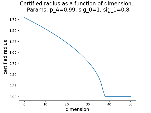
Figure 11: The certified radius as a function of dimension. Paremeters are $p_{A}=0.99,\sigma_{0}=1,\sigma_{1}=0.8$

The key reason why this happens if done via Rényi divergences is that while the divergence
$D_{\alpha}(\mathcal{N}(x_{1},\sigma_{1}^{2}I)||\mathcal{N}(x_{0},\sigma_{0}^{2}I))$ grows independently of dimension as $\lVert x_{0}-x_{1}\rVert$ grows, it drastically increases for big $N$ even if $x_{1}=x_{0}$! This reflects the effect, that if $\sigma_{0}\neq\sigma_{1}$, then the more dimensions we have, the more dissimilar are $\mathcal{N}(x_{1},\sigma_{1}^{2}I)$ and $\mathcal{N}(x_{0},\sigma_{0}^{2}I))$. We can think of it as a consequence of standard fact from statistics that the more data we have, the more confident statistics against the null hypothesis $\sigma_{0}=\sigma_{1}$ will we get if the null hypothesis is false. Since isotropic normal distributions can be actually treated as a sample of one-dimensional normal distributions, this is in accordance with our multivariate distributions setting.

B.2 The Explanation of the Curse of Dimensionality

In the Section 2 we show that input-dependent RS suffers from the curse of dimenisonality. Now we will elaborate a bit more on this phenomenon and try to explain why it occurs. First, it is obvious from the Subsection B.1, that also the generalized method of (Li et al., 2019) suffers from the curse of dimensionality, because the Rényi divergence between two isotropic Gaussians with different variances grows considerably with respect to dimension. This suggests that the input-dependent RS might suffer from the curse of dimensionality in general. To motivate this idea even further, we present this easy observation:

Theorem B.6.

Denote $R_{C}$ to be a certified radius given for $p_{A}$ and $\sigma_{0}$ at $x_{0}$ assuming the constant $\sigma_{0}$ and following the certification of (Cohen et al., 2019) . Assume, that we do the certification for each $x_{1}$ by assuming the worst case-classifier as in Theorem 2.2. Then, for any $x_{0}$, any function $\sigma(x)$ and any $p_{A}$, the following inequality holds:

$$R\leq R_{C}$$

Proof.

Fix $x_{1}$ and $\sigma_{1}$. From Theorem 2.2 we know that the worst-case classifier $f^{*}$ defines a ball $B$ such that $\mathbb{P}_{0}(B)=1-p_{A}$. From this it obviously follows, that the linear classifier $f_{l}$ and the linear space $B_{l}$ that assume constant $\sigma_{0}$ also for $x_{1}$ and is the worst-case for $\sigma_{0}$ such that $\mathbb{P}_{0}(B_{l})=1-p_{A}$ is not worst-case for the case of using $\sigma_{1}$ instead. Therefore, $\mathbb{P}_{1}(B_{l})\leq\mathbb{P}_{1}(B)$.

Moreover, let $\mathbb{P}_{1}^{C}$ be a probability measure corresponding to $\mathcal{N}(x_{1},\sigma_{0}I)$, i.e. the probability measure assuming constant $\sigma_{0}$. It is easy to see that $\mathbb{P}_{1}^{C}(B_{l})>0.5\iff\mathbb{P}_{1}(B_{l})>0.5$ because the probability of a linear half-space under isotropic normal distribution is bigger than half if and only if the mean is contained in the half-space.

Assume, for contradiction that $R>R_{C}$. From that, it exists a particular $x_{1}$ such that $\mathbb{P}_{1}^{C}(B_{l})>0.5>\mathbb{P}_{1}(B)$, because otherwise there would be no such point, which would cause $R>R_{C}$. However, $\mathbb{P}_{1}^{C}(B_{l})>0.5\implies\mathbb{P}_{1}(B_{l})>0.5$, thus $\mathbb{P}_{1}(B_{l})>\mathbb{P}_{1}(B)$ and that is contradiction. ∎

This theorem shows, that we can never achieve a better certified radius at $x_{0}$ using $\sigma_{0}$ and having probability $p_{A}$ than that, which we would get by (Cohen et al., 2019)’s certification. Of course, this does not mean, that using non-constant $\sigma$ is useless, since $\sigma_{0}$ can vary. The question is, how much do we lose using non-constant $\sigma$. To get a better intuition, we plot the functions $\xi_{<}$ and $\xi_{>}$ under different setups in Figure 12, together with $\mathbb{P}_{1}(B_{l})$ from the proof of Theorem B.6. From the top row we can deduce that dimension $N$ has a very significant impact on the probabilities and therefore also on the certified radius. We particularly point out the fact, that even $\xi_{>}(0),\xi_{<}(0)$ can have significant margin w.r.t. to the probability coming out of linear classifier. Already for $N=90$, we are not able to certify $p_{A}=0.99$ for rather conservative value of $\frac{\sigma_{0}}{\sigma_{1}}$. From middle row we see, that decreasing $\frac{\sigma_{0}}{\sigma_{1}}$ can mitigate this effect strongly. For instance, for $\sigma_{0}=1,\sigma_{1}=0.95$ the difference between $\mathbb{P}_{1}(B)$ and $\mathbb{P}_{1}(B_{l})$ is almost negotiated. Bottom row compares $\xi_{>}(a),\xi_{<}(a)$ and the respective linear classifier probabilities. We can see, that the case $\sigma_{0}<\sigma_{1}$ might cause stronger restrictions on our certification (yet we deduce it just form the picture).

What is the reason for $\xi_{>}(a),\xi_{<}(a)$ being so big even at 0? The problem is following: Assume $\sigma_{0}>\sigma_{1}$. If $x_{0}=x_{1}$, the worst-case classifier coming from Lemma 2.2 will be a ball $B$ centered right at $x_{0}$, such that $\mathbb{P}_{0}(B)=1-p_{A}$. If we look at $\mathbb{P}_{1}(B)$, we see, that we have the same ball centered directly at the mean, but the variance of the distribution is smaller. Using spherical symmetry of the isotropic gaussian distribution, this is equivalent to evaluating the probability of a bigger ball. If we fix $\frac{\sigma_{0}}{\sigma_{1}}$ and look at the ratio of probabilities $\frac{\mathbb{P}_{1}(B)}{\mathbb{P}_{0}(B)}$ with increasing $N$, the curse of dimensionality comes into the game. For $N=2$, the ratio is not too big. However, if $N=3072$, like in CIFAR10, this ratio is far bigger. This can be intuitively seen from a property of chi-square distribution (which is present in the case $x_{0}=x_{1}$), that while expectation is $N$, the standard deviation is “just” $\sqrt{2N}$, i.e. $\frac{\sqrt{Var(\chi^{2}_{N})}}{\mathbb{E}(\chi^{2}_{N})}\xrightarrow[]{}0$ as $N\xrightarrow[]{}\infty$.

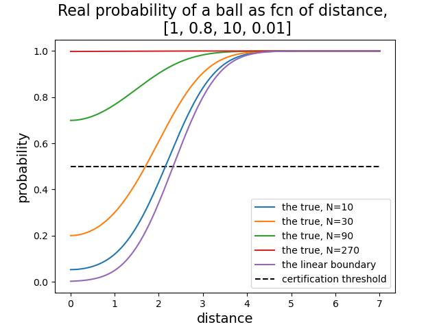
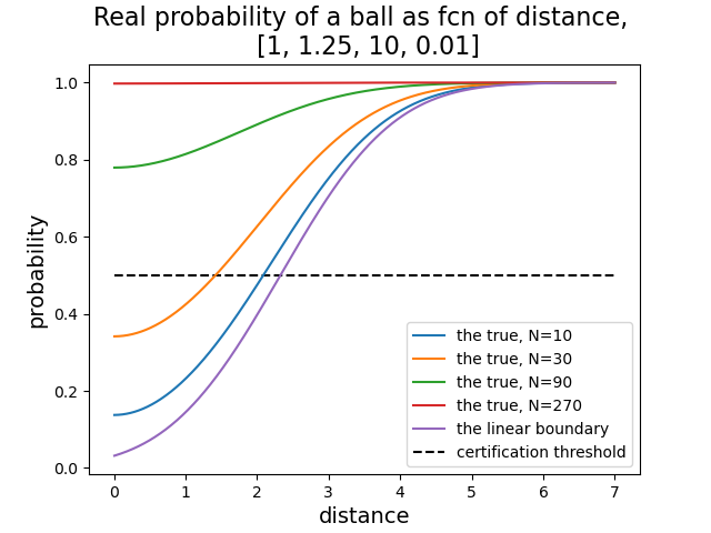
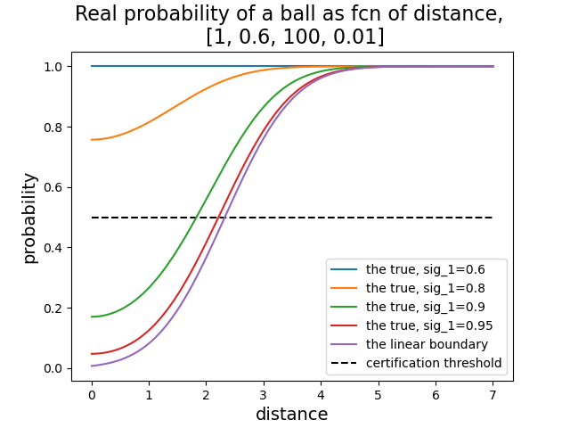
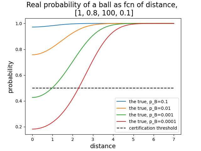
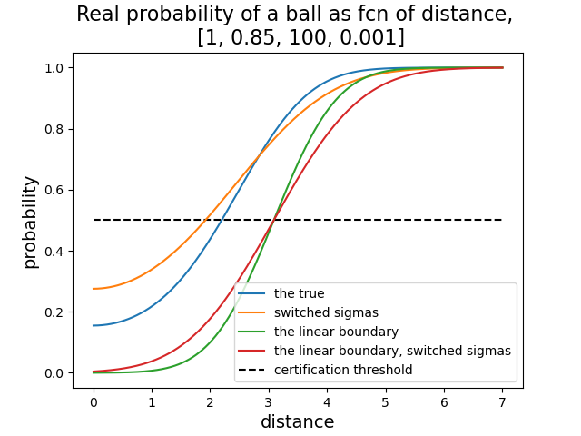
Figure 12: Plots of $\xi_{>}(a),\xi_{<}(a)$ for different setups. Coding for parameters is: $[\sigma_{0},\sigma_{1},N,p_{B}]$ Top: $\xi_{>}(a)$ left, $\xi_{<}(a)$ right, varying values of $N$. Center: On the left, $\xi_{>}(a)$ for varying $\sigma_{1}$, on the right $\xi_{>}(a)$ for varying $p_{B}$. Bottom: $\xi_{>}(a)$ and $\xi_{<}(a)$ compared.

B.3 Why Does the Input-dependent Smoothing Work Better for Small $\sigma$ Values?

As can be observed in Section 4 and Appendix LABEL:appE:_experiments_and_ablations, the bigger the $\sigma_{b}=\sigma$ we use, the harder it is to keep up to standards of constant smoothing. An interesting question is, why is the usage of small $\sigma_{b}=\sigma$ helpful for the input-dependent smoothing?

Assume fixed $\sigma$, say $\sigma_{b}=\sigma=0.12$. The theoretical bound on the certified radius given 100000 Monte-Carlo samplings and 0.001 confidence level using constant smoothing is about 0.48. Having $\sigma(x)\sim 0.12$, we cannot expect much bigger certified radius. Therefore, if we follow Theorem 3.2, the values of $\exp(-rR)$ and $\exp(rR)$ in the critical distance $\sim 0.5$ will be much closer to 1, than the values of $\exp(-rR)$ and $\exp(rR)$ if we used $\sigma_{b}=\sigma=0.50$ instead, where the critical values of $R$ could be much bigger than 0.5. Therefore, the “gain” in $\mathbb{P}_{1}(B)$ imposed by the curse of dimensionality, compared to $\mathbb{P}_{1}(B)$ assuming constant $\sigma$ will not be that severe yet. This means, that the loss in certified radius caused by the curse of dimensionality will be much less pronounced on the “active” range of certified radiuses (those for which the constant smoothing still works), compared to using big $\sigma_{b}=\sigma$. To support this idea, we demonstrate it on Figure 13, where we depict the certified radius as a function of distance from decision boundary, assuming $f$ to be a linear classifier, using $\sigma_{b}=\sigma=0.12$ and $\sigma_{b}=\sigma=0.50$ for comparison.

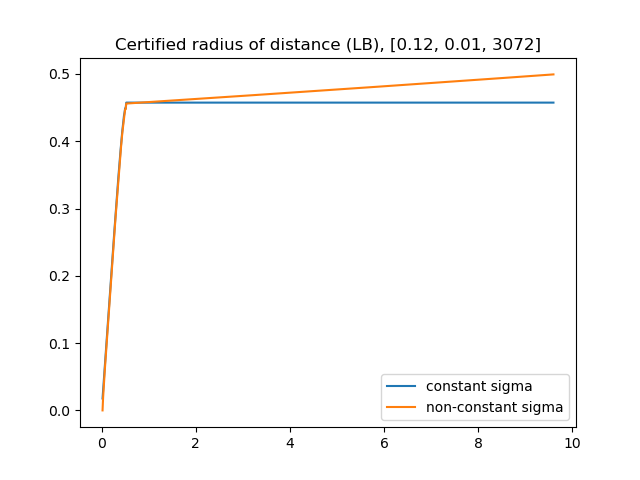
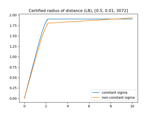
Figure 13: Comparison of certified radius as a function of distance for constant and input-dependent smoothing. Left: $\sigma_{b}=\sigma=0.12$, right: $\sigma_{b}=\sigma=0.50$.

B.4 How Does the Curse of Dimensionality Affect the Total Possible Variability of $\sigma(x)$?

Fix certain type of task, say RGB image classification with images of similar object, but consider many possible resolutions (dimensions $N$). Given two random images from the test set ($x_{0},x_{1}$), what is the biggest reasonable value of $|\sigma(x_{0})/\sigma(x_{1})-1|$? Theoretically, the expression is bounded by $|\exp(\pm r\lVert x_{0}-x_{1}\rVert)-1|$, given that $r$ is the semi-elasticity constant of $\sigma(x)$. However, the average distance between two samples from a test set of constant size, but increasing dimension scales as $\sqrt{N}$. Therefore, with constant $r$, this upper-bound increases.

The increasing distance between samples is, therefore, a countereffect to the curse of dimensionality. In simple words, we have “more distance to change $\sigma(x_{0})$ to $\sigma(x_{1})$”. Even if the $r$ decreased just as $1/\sqrt{N}$, the increasing distances would cancel the effect of the curse of dimensionaity and as a result, the maximal reasonable value of $|\sigma(x_{0})/\sigma(x_{1})-1|$ would remain roughly constant w.r.t. $N$. However, we need to take into account another effect. As the dimension increases, also the average distance of samples from the decision boundary increases. This is because the distances in general grow with dimension and if we assume that the number of intersections of a line segment between $x_{0}$ and $x_{1}$ with the decision boundary of the network remains roughly constant then the average distance from the decision boundary grows as $\sqrt{N}$ too. In order to compensate for this, we need to adjust the basic level of $\sigma(x)$ (which we later call $\sigma_{b}$ and can be understood as the general offset of our $\sigma(x)$) as $\sqrt{N}$ too. This is because the maximal attainable certified radius given fixed confidence level $\alpha$ and the number of Monte-Carlo samples is a constant multiple of $\sigma(x)$.

However, with increased $\sigma$, we need to decrease the semi-elasticity rate $r$ in order to obtain full certifications (see also Appendix B.3 for intuition behind this).

As a sketch of proof, we provide a simple computation, which tells us the approximate asymptotic behavior of $|\sigma(x_{0})/\sigma(x_{1})-1|$. By Theorem 2.5 it holds:

$$\exp(-rc\sqrt{N})\geq\sqrt{1-2\sqrt{\frac{-\log(p_{B})}{N}}},$$

if we want to be able to predict a certified radius of $c\sqrt{N}$ (though this is just a necessary condition. For sufficiency, the LHS must be much closer to 1). After simple manipulation, we obtain:

$$r\leq-\frac{1}{2c\sqrt{N}}\log\left(1-2\sqrt{\frac{-\log(p_{B})}{N}}\right)\sim-\frac{1}{2c\sqrt{N}}(-1)2\sqrt{\frac{-\log(p_{B})}{N}}=\frac{\sqrt{-\log(p_{B})}}{cN}.$$

So the rate scales as $1/N$. Now we have:

$$|\sigma(x_{0})/\sigma(x_{1})-1|\leq|\exp(\pm r\lVert x_{0}-x_{1}\rVert)-1|\leq\exp(r\lVert x_{0}-x_{1}\rVert)-1\leq$$

$$\exp(\frac{\sqrt{-\log(p_{B})}}{cN}C\sqrt{N})-1\sim\frac{\sqrt{-C\log(p_{B})}}{c\sqrt{N}}.$$

B.5 Does the Curse of Dimensionality Apply in Multi-class Regime?

In the main text, we presented a setup, where $\overline{p_{B}}$ is set to be $1-\underline{p_{A}}$. This is equivalent to pretending that we have just 2 classes. By not estimating the proper value of $p_{B}$ we lose some amount of power and the resulting certified radius is smaller than it could have been, did we have the $\overline{p_{B}}$ as well. This is most pronounced for datasets with many classes. The natural question, therefore, is, whether we could avoid the curse of dimensionality by properly estimating the $p_{B}$ together with $p_{A}$. The answer is no. The problem is that the the theory in Section 2 already implicitly works with the estimate of $p_{B}$ in a form of $1-\underline{p_{A}}$. The theory would work also with any other estimate of $p_{B}$. Assuming constant $p_{B}$, instead of constant $p_{A}$, as we did in Section 2, will, therefore, yield the same conclusions. Moreover, there is neither theoretical, nor practical reason, why should $p_{B}$ decrease with increasing dimension.

This insight even applies to the question of the usage of input-dependent RS in practice. The assumption $p_{B}=1-p_{A}$ is no more important in Section 3 than in Section 2. Therefore, we can apply our method also for the $\overline{p_{B}}$ obtained directly by Monte-Carlo sampling for the class $B$ (or by any other estimation method).

Appendix C Competitive Work

As we mention in Section 1, the idea to use input-dependent RS is not new. It has popped out in years 2020 and 2021 in at least four works from three completely distinct groups of authors, even though none of these works has been successfully published yet. We find it necessary to comment on all of these works because of two orthogonal reasons. First, it is a good practice to compare our work with the competitive work to see what are pros and cons of these similar approaches and to what extend the approaches differ. Second, we are convinced, that three of these four works claim results, which are not mathematically valid. We find this to be a particularly critical problem in a domain such as certifiable robustness, which is by definition based on rigorous, mathematical certifications.

C.1 The Work of Wang et al. (2021)

In this work, authors have two main contributions – first, they propose a two-phase training, where in the second phase, for each sample $x_{i}$, roughly the optimal $\sigma_{i}$ is being found and then this sample $x_{i}$ is being augmented with this $\sigma_{i}$ as an augmentation standard deviation. Authors call this method pretrain to finetune. Second, they provide a specific version of input-dependent RS. Essentially, they try to overcome the mathematical problems connected to the usage of non-constant $\sigma(x)$ by splitting the input space in so called robust regions $R_{i}$, where the constant $\sigma_{i}$ is guaranteed to be used. All the certified balls are guaranteed to lie within just one of these robust regions, making sure that within one certified region, constant level of $\sigma$ is used. Authors test this method on CIFAR10 and MNIST and show, that the method can outperform existing state-of-the-art approaches, mainly on the more complex CIFAR10 dataset.

However, we make several points, which make the results of this work, as well as the proposed method less impressive:

• The computational complexity of both their train-time and test-time algorithms seems to be quite high.

• The final smoothed classifier depends on the order of the incoming samples. As a consequence, it is not clear, whether the method works well for any permutation of the would-be tested samples. This creates another adversarial attack possibility - to attack the final smoothed classifier by manipulating the test set so that the order of samples is inappropriate for the good functionality of the final smoothed classifier.

• Even more, the fact, that the smoothed classifier depends on the order of the would-be tested samples makes it necessary, that the same smoothed classifier is used all the time for some test session in a real-world applications. For instance, a camera recognizing faces to approve an entry to a high-security building would need to keep the same model for its whole functional life, because restarting the model would enable attackers to create attacks on the predictions from the previous session. This might lead to significant restrictions on the practical usability of this method.

C.2 The Works of Alfarra et al. (2020) and Eiras et al. (2021)

In these works, similarly as in the work of (Chen et al., 2021), authors suggest to optimize in each test point $x$ for such a $\sigma(x)$, that maximizes the certified radius given by (Zhai et al., 2020), which is an extension of (Cohen et al., 2019)’s certified radius for soft smoothing. The optimization for $\sigma(x)$ differs but is similar in some respect (as will be discussed).

Besides, all three works further propose input-dependent training procedure, for which $\sigma(x)$ - the standard deviation of gaussian data augmentation is also optimized. Altogether, both authors claim strong improvements over all the previous impactful works like (Cohen et al., 2019; Zhai et al., 2020; Salman et al., 2019). The only significant difference between the works of (Alfarra et al., 2020) and (Eiras et al., 2021) (which have strong author intersections) is that in (Eiras et al., 2021), authors build upon (Alfarra et al., 2020)’s work and move from the isotropic smoothing to the smoothing with some specific anisotropic distributions.

As mentioned, authors first deviate from the setup of (Cohen et al., 2019) and turn to the setup introduced by (Zhai et al., 2020), i.e. they use soft smoothed classifier $G$ defined as

$${G_{F}(x)}_{C}=\mathbb{E}_{\delta\sim\mathcal{N}(0,\sigma^{2}I)}F(x+\delta)_{C}.$$

The key property of soft smoothed classifiers is that the (Cohen et al., 2019)’s result on certified radius holds for them too.

Theorem C.1 (certified radius for soft smoothed classifiers).

Let $G$ be the soft smoothed probability predictor. Let $x$ be s.t.

$$G(x)_{A}\geq\underline{E_{A}}\geq\overline{E_{B}}\geq G(x)_{B}.$$

Then, the smoothed classifier $g$ is robust at $x$ with radius

$$R=\frac{\sigma}{2}(\Phi^{-1}(\underline{E_{A}})-\Phi^{-1}(\overline{E_{B}}))=\sigma\frac{\Phi^{-1}(\underline{E_{A}})+\Phi^{-1}(1-\overline{E_{B}}))}{2},$$

where $\Phi^{-1}$ denotes the quantile function of standard normal distribution.

Proof.

Is provided in (Zhai et al., 2020). ∎

Note, that it is, similarly as in the hard randomized smoothing version of this theorem, essential to provide lower and upper confidence bounds for $G(x)_{A}$ and $G(x)_{B}$, otherwise we cannot use this theorem with the required probability that the certified radius is valid. Denote $G(x,\sigma)$ to be the soft smoothed classifier using $\sigma$ in $x$. Authors propose to use the following theoretical $\sigma(x)$ function:

$$\sigma(x)=\underset{\sigma>0}{\arg\max}\frac{\sigma}{2}(\Phi^{-1}(G(x,\sigma(x))_{A})-\Phi^{-1}(G(x,\sigma(x))_{B})).$$ (2)

It is of course not possible to optimize for this particular function since it is not known. It is also not feasible to run the Monte-Carlo sampling for each $\sigma$, because that is too costly and moreover due to stochasticity, it would lead to discontinuous function. Treatment of this problem is probably the most pronounced difference between the works of (Alfarra et al., 2020) and (Chen et al., 2021).

(Alfarra et al., 2020) use the following easy observation: $\mathcal{N}(0,\sigma^{2}I)\equiv\sigma\mathcal{N}(0,I)$. Assume we have $\delta_{i},i\in\{1,\dots,M\}$ be i.i.d. sample from $\mathcal{N}(0,I)$. Obviously, $G(x,\sigma(x))_{A}\sim\frac{1}{M}\sum\limits_{i=1}^{M}F(x+\sigma\delta_{i})_{A},$ since this is just the empirical mean of the theoretical expectation. Then, Expression 2 can be approximated as:

$$\sigma(x)=\underset{\sigma>0}{\arg\max}\frac{\sigma}{2}\left(\Phi^{-1}\left(\frac{1}{M}\sum\limits_{i=1}^{M}F(x+\sigma\delta_{i})_{A}\right)-\Phi^{-1}\left(\frac{1}{M}\sum\limits_{i=1}^{M}F(x+\sigma\delta_{i})_{B}\right)\right).$$ (3)

Here, $M$ is the number of Monte-Carlo samplings used to approximate this function. Note, that this function is a random realization of stochastic process in $\sigma$ which is driven by the stochasticity in the sample $\delta_{i},i\in\{1,\dots,M\}$. To find the maximum of this function, authors furhter propose to use simple gradient ascent, which is possible due to the simple differentiable form of Expression 3. This differentiability is one of the main motivations to switch from hard to soft randomized smoothing. Now, we are able to state the exact optimization algorithm of (Alfarra et al., 2020):

Algorithm 1 Data dependent certification (Alfarra et al., 2020)

OptimizeSigma$F,x,\beta,\sigma_{0},M,K$: $k=0,\dots,K$$\text{sample}\hskip 2.84526pt\delta_{1},\dots,\delta_{M}\sim\mathcal{N}(0,I)$$\phi(\sigma_{k})=\frac{1}{M}\sum\limits_{i=1}^{M}F(x+\sigma\delta_{i})$$\hat{E}_{A}(\sigma_{k})=\max_{C}\phi(\sigma_{k})_{C}$$\hat{E}_{B}(\sigma_{k})=\max_{C\neq A}\phi(\sigma_{k})_{C}$$R(\sigma_{k})=\frac{\sigma_{k}}{2}(\Phi^{-1}(\hat{E}_{A}(\sigma_{k}))-\Phi^{-1}(\hat{E}_{B}(\sigma_{k})))$$\sigma_{k+1}\leftarrow\sigma_{k}+\beta\nabla_{\sigma_{k}}R(\sigma_{k})$$\sigma^{*}=\sigma_{K}$$\sigma^{*}$

Note, that being done in this way, this algorithm can be viewed as a stochastic gradient ascent. After obtaining $\sigma^{*}\equiv\sigma(x)$, authors further run the Monte-Carlo sampling to estimate the certified radius exactly as in (Cohen et al., 2019), but with $\sigma(x)$ instead of some global $\sigma$. Using this algorithm, authors achieve significant improvement over the (Cohen et al., 2019)’s results, particularly getting rid of the first problem mentioned in Appendix A, the truncation issue. For the results, we refer to (Alfarra et al., 2020). We will now give several comments on this algorithm and this method.

To begin with, in this optimization, authors do not adjust the estimated expectations and therefore don’t use lower confidence bounds, but rather raw estimates. This is not incorrect, since these estimates are not used directly for the estimation of certified radius, but it is inconsistent with the resulting estimation. In other words, authors optimize for a slightly different function than they then use. The difference is, however, not very big apart from extreme values of $E_{A}$, where the difference might be really significant.

To overcome slightly this inconsistence, authors further (without comment) use clamping of the $\hat{E}_{A}(\sigma_{k})$ and $\hat{E}_{B}(\sigma_{k})$ on the interval $[0.02,0.98]$. I.e. if $\hat{E}_{A}(\sigma_{k})>0.98$, it will be set to $0.98$ and this is also taken into account in the computation of gradients. This way, authors get rid of the inconvenient issue, that if $G(x)_{A}\sim 1$, then $\hat{E}_{A}(\sigma_{k})\sim 1$ for $\sigma_{k}\sim 0$, what might cause very big value of $\Phi^{-1}(\hat{E}_{A}(\sigma_{k}))$, yielding strong inconsistency with what would be obtained, if lower confidence bound was used instead.

However, the clamping causes even stronger inconsistence in the end. Note, that if $G(x)_{A}\sim 1$, then the true value of $E_{A}(\sigma_{k})$ would be really close to $1$, yielding high values of $\Phi^{-1}(E_{A}(\sigma_{k}))$. This value would be far better approximated by the lower confidence bound than with the clamping, since the lower confidence bound of 1 for $M=100000$ and $\alpha=0.001$ is more than $0.9999$, while the clamped value is just $0.98$. This makes small values of $\sigma$ highly disadvantageous, since $\frac{\sigma}{2}\xrightarrow[]{}0$ as $\sigma\xrightarrow[]{}0$, yet $\Phi^{-1}(\hat{E}_{A}(\sigma_{k}))$ is being stuck on $\Phi^{-1}(0.98)$. In other words, this way authors artificially force the resulting $\sigma(x)$ to be big enough, s.t. $E(\sigma(x))_{A}\leq 0.98$. This assumption is not commented in the article and might result in intransparent behaviour.

Second of all, authors use $M=1$ for their experiments. This can be interpreted as using batch size 1 in classical SGD. We suppose that this small batch size is suboptimal since it yields an insanely high variance of the gradient.

Third of all, during the search for $\sigma(x)$, it is not taken into account, whether the prediction is correct or not. This is, of course, a scientifically correct approach, since we cannot look at the label of the test sample before the very final evaluation. However, it is also problematic, since the function in Expression 2 might attain its optimum in such a $\sigma(x)$, which leads to misclassification. This could have been avoided if constant $\sigma$ was used instead.

To further illustrate this issue, assume $F(x)=\mathbf{1}(B_{1}(0))$, i.e. $F(x)$ predicts class 1 if and only if $\lVert x\rVert\leq 1$, otherwise predicts class 0. Assume we are certifying $x\equiv 0$ and assume that $\sigma_{0}$ in Algorithm 1 is initialized such that class 0 is already dominating. Then, we will have positive gradient $\nabla_{\sigma_{k}}R(\sigma_{k})$ in all steps, because $F(\sigma\delta_{i})$ is obviously non-increasing, so the number of points classified as class 1 for fixed sample $\delta_{i},i\in 1,\dots,M$ is decreasing, yielding $\hat{E}_{A}(\sigma_{k})$ non-decreasing in $\sigma_{k}$, while $\frac{\sigma_{k}}{2}$ strictly increasing in $\sigma_{k}$. This way, the $\sigma_{k}$ will diverge to $\infty$ for $k\xrightarrow[]{}\infty$. However, point $x\equiv 0$ is classified as class 1, yielding misclassification which is, moreover, assigned very high certified radius.

This issue is actually even more general - the function in Expression 2 does in most cases (assuming infinite region $\mathbb{R}^{N}$) not possess global maximum, because usually

$$\underset{\sigma\xrightarrow[]{}\infty}{\lim}\frac{\sigma}{2}(\Phi^{-1}(G(x,\sigma(x))_{A})-\Phi^{-1}(G(x,\sigma(x))_{B}))=\infty.$$

This can be seen, for instance, easily for the $F(x)=\mathbf{1}(B_{1}(0))$, but it is the case for any hard classifier, for which one region becomes to have dominating area as the radius around some $x_{0}$ goes to infinity. This is because, if some region becomes to be dominating (for instance if all other regions are bounded), then $\frac{\sigma}{2}$ grows, while $\Phi^{-1}(G(x,\sigma(x))_{A})-\Phi^{-1}(G(x,\sigma(x))_{B})$ either grows too, or stagnates, making the whole function strictly increasing with sufficiently high slope.

This issue also throws the hyperparameter $K$ under closer inspection. What is the effect of this hyperparameter on the performance of the algorithm? From the previous paragraph, it seems, that this parameter serves not only as the “ scaled number of epochs”, but also as some stability parameter, which, however, does not have theoretical, but rather practical justification.

Another issue is, that the function in Expression 2 might be non-convex and might possess many different local minima, from which not all (or rather just a few) are actually reasonable. Therefore, the Algorithm 1 is very sensitive to initialization $\sigma_{0}$.

However, probably the biggest issue of all is connected to the impossibility result showed in Section 2, which shows, that the Algorithm 1 actually yields invalid certified radiuses. Why it is so?

First of all, we must justify, that our impossibility result is applicable also for the soft randomized smoothing. This is because classifiers of type $F(x)_{C}=\textbf{1}(x\in R_{C})$ for $R_{C}$ being decision region for class $C$ are among applicable classifiers s.t. $G(x,\sigma)_{A}=E_{A}$. With such classifiers, however, there is no difference between soft and hard smoothing and moreover $E_{A}\equiv p_{A}$ from our setup. This way we can construct the worst-case classifiers $F^{*}$ exactly as in our setup and therefore the same worst-case classifiers and subsequent adversarial examples are applicable here as well. In other words, for fixed value of soft smoothed $G(x,\sigma)_{A}=E_{A}$ we can denote $p_{A}=E_{A}$ and find the worst-case hard classifier $F$ defined as indicator of the worst-case ball, which will yield $E_{B}\equiv\mathbb{P}_{1}(B)$ from Theorem 2.3 in some queried point $x_{1}$.

As we have seen in previous paragraphs, the resulting $\sigma(x)$ yielded in Algorithm 1 is very instable and stochastic - it depends heavily on $F,\sigma_{0},K,\beta,M$ and of course $\delta_{i},i\in\{1,\dots,M\}$ for each iteration of the for cycle. Now, for instance for CIFAR10 and $p_{A}=0.99$, we have the minimal possible ratio $\frac{\sigma_{0}}{\sigma_{1}}$ equal to more than $0.96$. It is hard to believe, that such instable, highly stochastic and non-regularized (except for $K,\beta$) method will yield $\sigma(x)$ sufficiently slowly varying such that within the certified radius around $x_{0}$, there will be no $x_{1}$ for which $\sigma_{1}$ deviates more than by this strict threshold from $\sigma_{0}$. This is even more pronounced on ImageNet, where the minimal possible ratio $\frac{\sigma_{1}}{\sigma_{0}}$ is above 0.99 for any $p_{A}$ or $E_{A}$.

Even without the help of curse of dimensionality, we can construct a counterexample for which the algorithm will not yield valid certified radius. Assume again $F(x)=\mathbf{1}(B_{1}(0))$ and assume modest dimension $N=2$. Assume we try to certify point $x_{0}\equiv[50,0]$. Then, the theoretical $\sigma$-dependent function from Equation 2 is depicted on Figure 14.

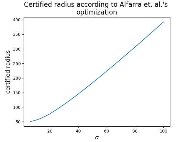
Figure 14: The theoretical certified radius as in Expression 2. The function is monotonically increasing on interval $[0,100]$ and will further be increasing too.

We can see, that the resulting $\sigma(x_{0})$ will be as big as our regularizers $K$ and $\beta$ in Algorithm 1 will allow. Therefore, if we run the algorithm for $K$ high-enough, surely the resulting certified radius will be far bigger than 50. However, if we certify the point $x_{0}\equiv[0,0]$ and we start with $\sigma_{0}=0.25$, for instance, then the $\sigma$-dependent certified radius in Expression 2 will be decreasing in this $\sigma_{0}$, yielding $\sigma(x_{0})<0.25$, which will result in classification of class 1. This point $[0,0]$ lies within the “certified” range of $[50,0]$, yet it is not classified the same, because, obviously, $[50,0]$ is classified as class 0. This is therefore a counterexample to the validity of (Alfarra et al., 2020)’s certification method and their results.

Note that even though our counterexample is a bit “extreme” and one could argue that in practice such a situation would not occur, we must emphasize, that this counterexample is constructed even without the help of the curse of dimensionality. In practice, it fully suffices, that for $x_{0}$ and some certified radius $R$ in $x_{0}$, there exists $x_{1}$ within the range of this certified radius, s.t. $\sigma_{1}$ is quite dissimilar to $\sigma_{0}$. If such situation occurs, then $R$ surely is not a valid certified radius.

Remark C.2.

In the latest version of their work, the authors themselves point out the issue outlined here. To overcome this issue, the authors further propose the following fix. Let test set be $\{x_{i}\}_{i=1}^{d}$. The samples are being processed consecutively from 1 to $d$. After obtaining a radius $R_{i}$ for a sample $x_{i}$, they “reserve” the ball around $x_{i}$ with radius $R_{i}$ so that every point falling in this ball from now on will be classified the same class as $x_{i}$. They also adjust a newly-computed certified radius $R_{j}$ of a sample $x_{j}$ so that the ball around $x_{j}$ doesn’t intersect with any previously reserved ball $x_{i},\hskip 2.84526pti<j$. If the sample falls into the already reserved region, the prediction on this sample is being forced to be the prediction of the sample in the region, and the certified radius is set such that the ball around the new sample is a subset of a ball reserved by the old sample.

Let us note that this fix by far does not solve the issues. Technically, it partially gets rid of the mathematical invalidity of certified radiuses, since now we at least have a guarantee that within the session for which we store all the previous test samples, there will be no direct violations of the certificates. However, this fix brings many other subtle and serious problems.

• Similarly as in Wang et al. (2021) it does depend on the order of incoming samples, creating possibilities for new adversarial attacks. To compare fairly, one would need to compare this method taking the worst possible certified accuracy result from all orderings of the test set.

• This method requires storing all the previously checked test samples, which might be a really big burden in some inference-heavy applications such as autonomous driving, but also many others.

• The classical randomized smoothing or also our framework provide guarantees which are session-agnostic. In other words, given a fixed model $f$ and a fixed variance function $\sigma(x)$ (possibly constant), the certified radius for a sample $x_{0}$ holds anywhere in the world at any time, on any device. Yet the model of Alfarra et al. (2020) requires synchronization of all the testing devices and if this synchronization is not provided then the guarantees hold just locally. Imagine our cell phones use some fixed classifier. If the phones were not synchronized, then within the certified radius around $x_{0}$ provided by one phone, there might be an adversarial example in some other phone.

• Probably the biggest issue is that the method uses a formula for the computation of certified radiuses which completely loses its meaning when the guarantees are actually based just on the fix. The Cohen et al. (2019)’s formula for certified radius is completely tailored for constant smoothing and used in this way it is just a random formula. A very simple and naive method would outperform everything existent. It just suffices to classify with $f$ or $g$ created with very small, constant $\sigma$ and then give constant certified radius to all the samples, computed such that given the size of the test set (which is known for instance in scientific comparisons) and the average distances between closest samples, we would choose radius which is just small enough to statistically not create intersections of certified regions. For instance for CIFAR10 and 10000 test samples, certified radiuses of 4 or 5 would be completely safe and wouldn’t create possibly any intersections. However, it is clear that such a method doesn’t make sense.

Why this method is so appealing at the first sight? The problem is that in practical comparisons on CIFAR or MNIST, there are no clashes of certified regions. That would not be the case if the test sets would be bigger. The average distance from the closest neighbor goes as $\frac{1}{\sqrt{d}}$ where $d$ is the number of samples.

One could argue that there might be something as “blessing of dimensionality”. The distances between samples grow with dimension and so the chance of clashes is smaller and smaller and thus extremely big amounts of test data would be needed to create some problems. However, this is not correct reasoning since with growing dimension, also the required $\sigma$ grows to provide appropriately big certified radiuses. From this point of view, the amount of test samples necessary to create troubles is roughly constant with respect to dimension and depends just on the topology of the data distribution.

C.3 The Work of Chen et al. (2021)

The methodology of (Chen et al., 2021) is rather similar to that of (Alfarra et al., 2020). The biggest difference consists in the optimization of Expression 2.

Instead of stochastic gradient descent, they use more sophisticated version of grid search - so called multiple-start fast gradient sign search. Simply speaking, this method first generates a set of pairs $(\sigma_{0},s)_{i},i\in\{1,\dots,K\}$ and then for each of the $i$ runs, it runs a $j$-while cycle, where in each step $j$, it increases $\sigma_{j}^{2}=\sigma_{0}^{2}+js$ to $\sigma_{j+1}^{2}=\sigma_{0}^{2}+(j+1)s$ and checks, whether the $\sigma$-dependent empirical certified radius in Expression 3 increases or not. If yes, they continue until $j$ is above some threshold $T$, if not, they break and report $\sigma_{i}$ as the $\sigma_{j}$ from the inner step where while cycle was broken. After obtaining $\sigma_{i}$ for $i\in\{1,\dots,K\}$, they choose $\sigma(x)$ to be the one, that maximizes Expression 3. More concretely, their multiple-start fast gradient sign search algorithm looks as follows:

Algorithm 2 Instance-wise multiple-start FGSS (Chen et al., 2021)

OptimizeSigma$F,x,\sigma_{0},M,K,T$: $\text{generate}\hskip 2.84526pt(l_{k},s_{k}),k\in\{1,\dots,K\}$$k=1,\dots,K$$\text{sample}\hskip 2.84526pt\delta_{1},\dots,\delta_{M}\sim\mathcal{N}(0,l_{k}\sigma_{0}^{2}I)$$\phi(\sqrt{l_{k}}\sigma_{0})=\frac{1}{M}\sum\limits_{i=1}^{M}F(x+\delta_{i})$$\hat{E}_{A}(\sqrt{l_{k}}\sigma_{0})=\max_{C}\phi(\sqrt{l_{k}}\sigma_{0})_{C}$$R(\sqrt{l_{k}}\sigma_{0})=\sqrt{l_{k}}\sigma_{0}\Phi^{-1}(\hat{E}_{A}(\sqrt{l_{k}}\sigma_{0}))$$m_{k}=R(\sqrt{l_{k}}\sigma_{0})$$l_{k}\in[1,T]$$\text{sample}\hskip 2.84526pt\delta_{1},\dots,\delta_{M}\sim\mathcal{N}(0,(l_{k}+s_{k})\sigma_{0}^{2}I)$$\phi(\sqrt{l_{k}+s_{k}}\sigma_{0})=\frac{1}{M}\sum\limits_{i=1}^{M}F(x+\delta_{i})$$\hat{E}_{A}(\sqrt{l_{k}+s_{k}}\sigma_{0})=\max_{C}\phi(\sqrt{l_{k}+s_{k}}\sigma_{0})_{C}$$R(\sqrt{l_{k}+s_{k}}\sigma_{0})=\sqrt{l_{k}+s_{k}}\sigma_{0}\Phi^{-1}(\hat{E}_{A}(\sqrt{l_{k}+s_{k}}\sigma_{0}))$$R(\sqrt{l_{k}+s_{k}}\sigma_{0})\geq R(\sqrt{l_{k}}\sigma_{0})$$l_{k}\leftarrow l_{k}+s_{k}$$m_{k}=R(\sqrt{l_{k}+s_{k}}\sigma_{0})$break$\sigma(x)=\underset{k\in\{1,\dots,K\}}{\max}m_{k}$$\sigma(x)$

It is not entirely clear from the text of (Chen et al., 2021), how exactly are $l_{k},s_{k}$ sampled, but it is written there, that the interval for $l$ is $[1,16]$ and for $s$ it is $(-1,1)$. Moreover, the authors don’t provide the code and from the text, it seems, that they don’t use lower confidence bounds during the evaluation of certified radiuses, what we consider to be a serious mistake (if really the case). However, we add some comments to this method regardless of the lower confidence bounds.

Generally, this method possesses most of the disadvantages mentioned in Section C.2. They use the same function for optimization, the Expression 2 and its empirical version 3. This means, that the method suffers from having several local optima, having no global optimum in general (and in most cases with limit infinity). Similarly like before, here is also no control over the correctness of the prediction, i.e. many or all local optima might lead to misclassification.

On the other hand, in this paper authors use $M=500$ (the effective batch size), which is definitely more reasonable than $M=1$ as in (Alfarra et al., 2020). Furthermore, they use multiple initializations, making the optimization more robust and improving the chances to obtain global, or at least very good local minimum.

However, the main problem, the curse of dimensionality yielding invalid results is even more pronounced here. Unlike the “continuous approach” in (Alfarra et al., 2020), here authors for each $x_{0}$ sample just some discrete grid (more complex, since there are more initializations) of possible values of $\sigma(x)$. For instance, if $s=1$, then the smallest possible ratio between two consecutive $l$’s in the Algorithm 2 is $\sqrt{15}/4\sim 0.97$, making it impossible to certify some $x_{1}$ w.r.t. $x_{0}$ if for both $s=1$ and $l_{0}\neq l_{1}$ on ImageNet and also for a lot of samples on CIFAR10. Of course, the fact that $s$ is randomly sampled from $(-1,1)$ makes this counter-argumentation more difficult, but it is, again, highly unlikely that this highly stochastic method without control over $\sigma(x)$ would yield function with sufficiently small semi-elasticity. Therefore also the impressive results of (Chen et al., 2021) are, unfortunately, scientifically invalid.

Appendix D Implementation Details

Even though our algorithm is rather easy, there are some perks that should be discussed before one can safely use it in practice. First, we show the actual Algorithm LABEL:my_method_algo.

Algorithm 3 Pseudocode for certification and prediction of my method based on (Cohen et al., 2019)

# evaluate $g$at $x_{0}$PREDICT$f,\sigma_{0},x_{0},n,\alpha$: $\texttt{counts}\xleftarrow[]{}\text{SampleUnderNoise(}f,x_{0},n,\sigma_{0}\text{)}$$\hat{c}_{A},\hat{c}_{B}\xleftarrow[]{}\text{two top indices in }\texttt{counts}$$n_{A},n_{B}\xleftarrow[]{}\texttt{counts}(c_{A}),\texttt{counts}(\hat{c}_{B})$BinomPValue$(n_{A},n_{A}+n_{B},0.5)\leq\alpha$$\hat{c}_{A}$ABSTAIN
# certify the robustness of$g$around$x_{0}$CERTIFY$f,\sigma_{0},x_{0},n_{0},n,\alpha$: $\texttt{counts0}\xleftarrow[]{}\text{SampleUnderNoise(}f,x_{0},n_{0},\sigma_{0}\text{)}$$\hat{c}_{A}\xleftarrow[]{}\text{top index in }\texttt{counts0}$$\texttt{counts}\xleftarrow[]{}\text{SampleUnderNoise(}f,x_{0},n,\sigma_{0}\text{)}$$\underline{p_{A}}\xleftarrow[]{}\text{LowerConfBound}(\texttt{counts}[\hat{c}_{A}],n,1-\alpha)$$\underline{p_{A}}>1/2$prediction $\hat{c}_{A}$and radius ComputeCertifiedRadius($\sigma_{0},r,N,\underline{p_{A}},\text{num\_steps}$)

References

- Alfarra et al. (2020) Alfarra, M., Bibi, A., Torr, P. H., and Ghanem, B. Data dependent randomized smoothing. arXiv preprint arXiv:2012.04351, 2020.
- Anil et al. (2019) Anil, C., Lucas, J., and Grosse, R. Sorting out Lipschitz function approximation. In Chaudhuri, K. and Salakhutdinov, R. (eds.), Proceedings of the 36th International Conference on Machine Learning, volume 97 of Proceedings of Machine Learning Research, pp. 291–301. PMLR, 09–15 Jun 2019. URL http://proceedings.mlr.press/v97/anil19a.html.
- Athalye & Carlini (2018) Athalye, A. and Carlini, N. On the robustness of the cvpr 2018 white-box adversarial example defenses. arXiv preprint arXiv:1804.03286, 2018.
- Athalye et al. (2018) Athalye, A., Carlini, N., and Wagner, D. Obfuscated gradients give a false sense of security: Circumventing defenses to adversarial examples. In International conference on machine learning, pp. 274–283. PMLR, 2018.
- Baldock et al. (2021) Baldock, R., Maennel, H., and Neyshabur, B. Deep learning through the lens of example difficulty. Advances in Neural Information Processing Systems, 34:10876–10889, 2021.
- Biggio et al. (2013) Biggio, B., Corona, I., Maiorca, D., Nelson, B., Šrndić, N., Laskov, P., Giacinto, G., and Roli, F. Evasion attacks against machine learning at test time. In Blockeel, H., Kersting, K., Nijssen, S., and Železný, F. (eds.), Machine Learning and Knowledge Discovery in Databases, pp. 387–402, Berlin, Heidelberg, 2013. Springer Berlin Heidelberg. ISBN 978-3-642-40994-3.
- Carlini & Wagner (2017) Carlini, N. and Wagner, D. Adversarial examples are not easily detected: Bypassing ten detection methods. In Proceedings of the 10th ACM workshop on artificial intelligence and security, pp. 3–14, 2017.
- Chen et al. (2021) Chen, C., Kong, K., Yu, P., Luque, J., Goldstein, T., and Huang, F. Insta-rs: Instance-wise randomized smoothing for improved robustness and accuracy. arXiv preprint arXiv:2103.04436, 2021.
- Cohen et al. (2019) Cohen, J., Rosenfeld, E., and Kolter, Z. Certified adversarial robustness via randomized smoothing. In International Conference on Machine Learning, pp. 1310–1320. PMLR, 2019.
- Eiras et al. (2021) Eiras, F., Alfarra, M., Kumar, M. P., Torr, P. H., Dokania, P. K., Ghanem, B., and Bibi, A. Ancer: Anisotropic certification via sample-wise volume maximization. arXiv preprint arXiv:2107.04570, 2021.
- Eykholt et al. (2018) Eykholt, K., Evtimov, I., Fernandes, E., Li, B., Rahmati, A., Xiao, C., Prakash, A., Kohno, T., and Song, D. Robust physical-world attacks on deep learning visual classification. In Proceedings of the IEEE conference on computer vision and pattern recognition, pp. 1625–1634, 2018.
- Gao et al. (2020) Gao, Y., Rosenberg, H., Fawaz, K., Jha, S., and Hsu, J. Analyzing accuracy loss in randomized smoothing defenses. arXiv preprint arXiv:2003.01595, 2020.
- Goodfellow et al. (2014) Goodfellow, I. J., Shlens, J., and Szegedy, C. Explaining and harnessing adversarial examples. arXiv preprint arXiv:1412.6572, 2014.
- Gühring et al. (2020) Gühring, I., Raslan, M., and Kutyniok, G. Expressivity of deep neural networks. arXiv preprint arXiv:2007.04759, 2020.
- Hayes (2020) Hayes, J. Extensions and limitations of randomized smoothing for robustness guarantees. In Proceedings of the IEEE/CVF Conference on Computer Vision and Pattern Recognition Workshops, pp. 786–787, 2020.
- Hein & Andriushchenko (2017) Hein, M. and Andriushchenko, M. Formal guarantees on the robustness of a classifier against adversarial manipulation. In Guyon, I., Luxburg, U. V., Bengio, S., Wallach, H., Fergus, R., Vishwanathan, S., and Garnett, R. (eds.), Advances in Neural Information Processing Systems, volume 30. Curran Associates, Inc., 2017. URL https://proceedings.neurips.cc/paper/2017/file/e077e1a544eec4f0307cf5c3c721d944-Paper.pdf.
- Krizhevsky (2009) Krizhevsky, A. Learning multiple layers of features from tiny images, 2009. URL http://www.cs.toronto.edu/~kriz/learning-features-2009-TR.pdf.
- Kumar et al. (2020) Kumar, A., Levine, A., Goldstein, T., and Feizi, S. Curse of dimensionality on randomized smoothing for certifiable robustness. In International Conference on Machine Learning, pp. 5458–5467. PMLR, 2020.
- Kurakin et al. (2016) Kurakin, A., Goodfellow, I., and Bengio, S. Adversarial machine learning at scale. arXiv preprint arXiv:1611.01236, 2016.
- LeCun et al. (1999) LeCun, Y., Cortes, C., and Burges, C. J. The mnist database of handwritten digits, 1999. URL http://yann.lecun.com/exdb/mnist/.
- Lecuyer et al. (2019) Lecuyer, M., Atlidakis, V., Geambasu, R., Hsu, D., and Jana, S. Certified robustness to adversarial examples with differential privacy. In 2019 IEEE Symposium on Security and Privacy (SP), pp. 656–672. IEEE, 2019.
- Li et al. (2019) Li, B., Chen, C., Wang, W., and Carin, L. Certified adversarial robustness with additive noise. Advances in Neural Information Processing Systems, 32:9464–9474, 2019.
- Madry et al. (2017) Madry, A., Makelov, A., Schmidt, L., Tsipras, D., and Vladu, A. Towards deep learning models resistant to adversarial attacks. arXiv preprint arXiv:1706.06083, 2017.
- Mirman et al. (2018) Mirman, M., Gehr, T., and Vechev, M. Differentiable abstract interpretation for provably robust neural networks. In Dy, J. and Krause, A. (eds.), Proceedings of the 35th International Conference on Machine Learning, volume 80 of Proceedings of Machine Learning Research, pp. 3578–3586. PMLR, 10–15 Jul 2018. URL http://proceedings.mlr.press/v80/mirman18b.html.
- Mohapatra et al. (2020a) Mohapatra, J., Ko, C.-Y., Liu, S., Chen, P.-Y., Daniel, L., et al. Rethinking randomized smoothing for adversarial robustness. arXiv preprint arXiv:2003.01249, 2020a.
- Mohapatra et al. (2020b) Mohapatra, J., Ko, C.-Y., Weng, T.-W., Chen, P.-Y., Liu, S., and Daniel, L. Higher-order certification for randomized smoothing. Advances in Neural Information Processing Systems, 33, 2020b.
- Raghunathan et al. (2018) Raghunathan, A., Steinhardt, J., and Liang, P. Certified defenses against adversarial examples. In International Conference on Learning Representations, 2018.
- Robert (1990) Robert, C. On some accurate bounds for the quantiles of a non-central chi squared distribution. Statistics & probability letters, 10(2):101–106, 1990.
- Salman et al. (2019) Salman, H., Li, J., Razenshteyn, I. P., Zhang, P., Zhang, H., Bubeck, S., and Yang, G. Provably robust deep learning via adversarially trained smoothed classifiers. In NeurIPS, 2019.
- Szegedy et al. (2013) Szegedy, C., Zaremba, W., Sutskever, I., Bruna, J., Erhan, D., Goodfellow, I., and Fergus, R. Intriguing properties of neural networks. arXiv preprint arXiv:1312.6199, 2013.
- Tsuzuku et al. (2018) Tsuzuku, Y., Sato, I., and Sugiyama, M. Lipschitz-margin training: Scalable certification of perturbation invariance for deep neural networks. In Bengio, S., Wallach, H., Larochelle, H., Grauman, K., Cesa-Bianchi, N., and Garnett, R. (eds.), Advances in Neural Information Processing Systems, volume 31. Curran Associates, Inc., 2018. URL https://proceedings.neurips.cc/paper/2018/file/485843481a7edacbfce101ecb1e4d2a8-Paper.pdf.
- Van Erven & Harremos (2014) Van Erven, T. and Harremos, P. Rényi divergence and kullback-leibler divergence. IEEE Transactions on Information Theory, 60(7):3797–3820, 2014.
- Wang et al. (2021) Wang, L., Zhai, R., He, D., Wang, L., and Jian, L. Pretrain-to-finetune adversarial training via sample-wise randomized smoothing. 2021. URL https://openreview.net/forum?id=Te1aZ2myPIu.
- Weng et al. (2018) Weng, L., Zhang, H., Chen, H., Song, Z., Hsieh, C.-J., Daniel, L., Boning, D., and Dhillon, I. Towards fast computation of certified robustness for ReLU networks. In Dy, J. and Krause, A. (eds.), Proceedings of the 35th International Conference on Machine Learning, volume 80 of Proceedings of Machine Learning Research, pp. 5276–5285. PMLR, 10–15 Jul 2018. URL http://proceedings.mlr.press/v80/weng18a.html.
- Wong & Kolter (2018) Wong, E. and Kolter, Z. Provable defenses against adversarial examples via the convex outer adversarial polytope. In International Conference on Machine Learning, pp. 5286–5295. PMLR, 2018.
- Wu et al. (2021) Wu, Y., Bojchevski, A., Kuvshinov, A., and Günnemann, S. Completing the picture: Randomized smoothing suffers from the curse of dimensionality for a large family of distributions. In International Conference on Artificial Intelligence and Statistics, pp. 3763–3771. PMLR, 2021.
- Yang et al. (2020) Yang, G., Duan, T., Hu, J. E., Salman, H., Razenshteyn, I., and Li, J. Randomized smoothing of all shapes and sizes. In International Conference on Machine Learning, pp. 10693–10705. PMLR, 2020.
- Zhai et al. (2020) Zhai, R., Dan, C., He, D., Zhang, H., Gong, B., Ravikumar, P., Hsieh, C.-J., and Wang, L. Macer: Attack-free and scalable robust training via maximizing certified radius. arXiv preprint arXiv:2001.02378, 2020.