Optimizing quantum control pulses with complex constraints and few variables through Tensorflow

Abstract

Applying optimal control algorithms on realistic quantum systems confronts two key challenges: to efficiently adopt physical constraints in the optimization and to minimize the variables for the convenience of experimental tune-ups. In order to resolve these issues, we propose a novel algorithm by incorporating multiple constraints into the gradient optimization over piece-wise pulse constant values, which are transformed to contained numbers of the finite Fourier basis for bandwidth control. Such complex constraints and variable transformation involved in the optimization introduce extreme difficulty in calculating gradients. We resolve this issue efficiently utilizing auto-differentiation on Tensorflow. We test our algorithm by finding smooth control pulses to implement single-qubit and two-qubit gates for superconducting transmon qubits with always-on interaction, which remains a challenge of quantum control in various qubit systems. Our algorithm provides a promising optimal quantum control approach that is friendly to complex and optional physical constraints.

I Introduction

Potential ground-breaking quantum technologies, such as quantum computing, quantum sensing, and quantum metrology Steane (1998); Degen et al. (2017); Giovannetti et al. (2011), become more and more feasible with the tremendous progress of quantum control technology on various physical systems Naranjo et al. (2018); Basset et al. (2021); Rembold et al. (2020); Chen et al. (2021). Based on growing knowledge quantum systems interacting with the enviroment, multifarious approaches have been developed to improve the control precision Motzoi et al. (2009); Economou and Barnes (2015a); Deng et al. (2017); Doria et al. (2011); Deng et al. (2021); Long et al. (2021); Machnes et al. (2018). Eventhough, further optimizing quantum control still highly relies on numerical approaches Khaneja et al. (2005); Machnes et al. (2011); Ruschhaupt et al. (2012); Zahedinejad et al. (2014); Caneva et al. (2011); Machnes et al. (2018). Practical quantum optimal control (QOC) Ohtsuki et al. (2004); Lloyd and Montangero (2014); Ohtsuki and Nakagami (2008); Sundermann and de Vivie-Riedle (1999) should satisfy the requirements and constraints in the physical systems, such as more realistic Hamiltonian, maximal field strength, finite sampling rate, limited bandwidth Jerger et al. (2019); Hincks et al. (2015); Rol et al. (2020), etc. Also, for efficient calibration in experiments, the control field waveform should depend on as few variables as possible. Other than the physical considerations, the optimization algorithm ought to be fast and accurate and should be extensible to larger systems. As one of the most successful numerical optimization algorithms, GRAPE has been applied to many physical systems, including NMR qubits Khaneja et al. (2005); Tošner et al. (2009); Jones (2010); Ryan et al. (2009); Nielsen et al. (2007), superconducting qubits in 3D cavity Schutjens et al. (2013); Blais et al. (2020a); Allen et al. (2017); Blais et al. (2007, 2020b), nitrogen-vacancy (NV) centers in diamond Niemeyer (2013); Wang and Dobrovitski (2011); Rembold et al. (2020); Platzer et al. (2010), etc. However, adapting GRAPE to multiple realistic constraints remains challenging. Different from GRAPE, another numerical algorithm, CRAB has been proposed to generate smooth control waveforms, towards application in cold atoms van Frank et al. (2016). There are also many other proposed algorithms leading to promising applications Zahedinejad et al. (2014); Ruschhaupt et al. (2012); Niu et al. (2019a); Shu et al. (2016a)

Depending on how to parametrize the control field’s variables, QOC algorithms could be assorted into two classes: 1. Piecewise constant (PWC) discretizes the field pulse as a sequence of piecewise-constant field strength and the value of each piece as the optimization variable Machnes et al. (2011); Khaneja et al. (2005); Niu et al. (2019b); Kirchhoff et al. (2018); Larocca and Wisniacki (2020). Varying each variable causing local variation of the whole waveform hence local variation of the expectation function, which preserves the convexity of optimization landscape in this parameter space. And then gradient-based optimization could efficiently proceed Khaneja et al. (2005); Ruschhaupt et al. (2012); Zahedinejad et al. (2014); Niu et al. (2019b). A trade-off arises between inaccurate PWC dynamics for finite discretization rate and the cost of computing the gradients versus massive variables. Also, PWC waveforms are not smooth and could easily contain fast fluctuations. Filtering the optimized waveform in the post-optimization deforms the output pulses from optimum. 2. Chopped basis (CB) optimization uses parameters related to a finite set of basis expanding the control waveform. The basis are usually analytic functions such as Gaussian, tangential, or Fourier functions Caneva et al. (2011); Machnes et al. (2018), etc, which easily guarantees the smoothness of the optimized waveform. However, adding the physical constraints deforms the processed pulses in an unknown wayCaneva et al. (2011); Machnes et al. (2018), so the output pulses lose the analyticity. Furthermore, small change of one expansion coefficient leads to global deformation of the pulse waveform, and also coefficients of different bases affect differently. Therefore, the CB optimization landscape becomes non-convex. Alternatively, constraints could be incorporated into optimization with Lagrange multipliers but the calculation of the analytical differentiation brings in another source of complexity and difficulty Plick and Krenn (2015); Moore and Rabitz (2012); Shu et al. (2016a).

Here in this article, we propose a novel optimization algorithm, the Complex and Optional Constraints Optimization with Auto-differentiation (COCOA), to tackle the problems summarized above. The algorithm parametrizes the control waveform in the basis of truncated Fourier series, while the optimization performs the gradient in the convex landscape of PWC parameter space. The transformation between the aforementioned two parametrization systems is bridged via approximate discrete Fourier transformation (DFT) and inverse discrete Fourier transformation (iDFT). The advantage of combining these two parametrization systems is that all the pulse constraints can be incorporated in the optimization process instead of post-optimization. The application of DFT and iDFT within the optimization iteration introduces further physical advantages: 1. Hard bounds on the bandwidth by limiting the Fourier basis; 2. Definite expansion with pre-selected basis; 3. Analytical expression of output pulses with a small number of parameters for tuning. 4. Convenient application of pulse pre-distortion because the transfer/filter functions are in the frequency domainKelly et al. (2014); Rol et al. (2020, 2019). However, embedding these constraints and the transformation of parametrization systems into the optimization iteration raises extreme difficulty in solving the analytical gradient equations. We resolve this issue using auto-differentiation during one-round back-propagation process provided by TensorflowAbadi et al. (2016). With Tensorflow, the automatical calculation of gradient could be further extended to various physical systems. This paper explains in detail how COCOA works and presents some numerical results to demonstrate the efficiency and its advantage compared with GRAPE and CRAB.

This paper is organised as follows. First, we take an overview of quantum optimal control theories and numerical methods. In Sec. III we present the algorithmic description of COCOA and explain how it combines the advantages of two categories QOC approaches and perform an optimization task under complex and optional constraints. Then in Sec. IV, we apply COCOA to find optimal quantum-gate pulses for superconducting qubits with always-on interactions. We simulate two models: cavity mediated two-qubit system and direct capacitively-coupled systems. We demonstrate COCOA’s advantages by comparing with the representative algorithms GRAPE and CRAB of the two QOC categories. In Sec. V, we conclude this paper.

II Quantum Optimal Control

II.1 General formalism

We consider a general Hamiltonian in QOC problem as

$$H(t)=H_{d}+H_{c}(t)$$ (1)

where $H_{d}$ is the drift Hamiltonian of the system. $H_{c}(t)$ is the time-dependent Hamiltonian which is to be optimized to control the quantum system to undergo a desired time evolution. The dynamics of the system steered by the total Hamiltonian in Eq. (1) satisfied the Schr$\ddot{o}$dinger equation $|\dot{\psi}(t)\rangle=-iH(t)|\psi(t)\rangle$, with the time evolution operator satisfying $\dot{U}(t)=-iH(t)U(t)$, or an integral form $U(t)=\mathcal{T}e^{-i\int H(t)dt}$, where $\mathcal{T}$ is the time-ordering operator. A generic form of the control Hamiltonian is $H_{c}(t)=H_{c}(\{\Omega_{j}(t)\},t)$, where $\{\Omega_{j}(t)\}$ are a set of time-dependent control pulse to be optimized. In our examples presented later, $\{\Omega_{j}(t)\}$ are chosen to be the envelopes of microwave drives on qubits, where $j=1x,1y,2x,2y$, i.e. $1x$ means rotating around X axis for qubit 1. For different QOC problems, expectation function could be customized. A constrained optimization could be perform by combining penalty functions into the expectation function with Lagrange multipliers Shu et al. (2016b); Plick and Krenn (2015). In the specific examples discussed in this article, we study the performance of a quantum gate at final time $t=T$ as an average over all possible initial quantum states. It can be quantified by the average gate fidelity Pedersen et al. (2007) defined as

$$f=\frac{1}{d(d+1)}(Tr(MM^{{\dagger}})+|Tr(M)|^{2})$$ (2)

where $M=U_{tar}U_{T}$, $d$ is the dimension of the quantum system. Therefore, we use infidelity as the cost function to be minimized, i.e. $F=1-f$.

II.2 Realistic requirements

Traditional pulse optimization algorithms are confronted with many issues while applying to realistic systems. We summarize various realistic issues below and design the COCOA optimization to bridge the gap between numerical optimization and experimental applications.

1. Pulse pre-distortion. Pulse distortion as one of the major issues could take place in the following process Rabiner and Gold (1975): i) Pulse generation with finite sampling rates, which could be modeled as FIR filter. ii) Transmission of signal, where a IIR transfer function could be used to model the distortion. iii) Numerical distortion when post-processing the optimal pulse for the purposes such as smoothening, which could be modelled as the post-optimization filter function. Commonly, the processed pulse is not optimal any more. Pulse pre-distortion with inverse filter function could be applied in experiments to compensate these effectsChen (2018); Rol et al. (2020). Since the filter functions are in frequency domain, it would be much more convenient for pre-distortion if the numerical output pulse is an analytical function for frequency rather than in the PWC form.

2. Pulse constraints: Optimal pulses should satisfy various physical constraints, such as smoothness, finite bandwidth, bounded amplitude, starting and ending at some designated values, robustness to some randomness (e.g. noises), and so on. Post-processing the optimized pulses with constraints results in numerical pulse distortion mentioned above. So it is necessary to incorporate constraints into the optimization. However, efficiently adding pulse constraints to the optimization is challenging, because the gradient might be too complicated to compute. Traditionally, conditional expressions such as if-else paragraph could be added into the optimization solver. But this results in possible loopholes and low efficiency. So a better approach is still open for investigation.

3. Pulse parameters. Optimizing the pulse parameters in experiments is necessary and could become exponentially strenuous when the number of parameters grows. Therefore, it is desired to obtain optimal pulses with few parameters for experimental tune-ups.

4. Analyticity of the pulse. The analyticity is defined as explicit and analytical function or a definite summation of several analytical functions, which helps generating and tuning control pulses in experiments.

In this article, we will show how the COCOA algorithm is engineered to satisfy the above requirements efficiently. And we will test its performance via realistic optimization tasks.

III COCOA Algorithm

III.1 List of symbols

Symbol	Meaning
$j$	Index of control pulse $(1x,1y,2x,2y)$
$k$	Time slice index $(1,\dots,N)$
$\Omega[k]$	Control amplitude in time slice $k$
$\mathcal{C,M,E,F}$	Transform function for each node: pulse
	constraint, bandwidth control, evolution,
	cost function
$\Omega^{r}(t)$	Control pulse at iteration $r$
$N_{c}$	Number of Fourier components kept in
	optimized pulse
$R$	Number of iterations in optimization
$\alpha$	Learning rate
$\epsilon_{0}$	Tolerance of cost function
$\epsilon_{1}$	Tolerance of gradient norm
$T$	Total gate time
$S_{0}$	Initial state
$S_{T}$	State at time $t=T$
$U_{T}$	Evolution operator at time $t=T$
$U_{tar}$	Target operator
$\Omega_{j}^{\ast}(t)$	Optimized pulse of $j$-th control

III.2 Pseudo code

The pseudo code of COCOA algorithm can be seen in Algorithm 1.

Algorithm 1 Complex and Optional Constraints Optimization (COCOA) for pulse engineering

1:cost function: $F$; initial pulse sequence: $\Omega_{j}^{0}(t)$; $N_{c}$; $\alpha$; Iterations: $R$; $\epsilon_{0}$; $\epsilon_{1}$

2:optimized pulse: $\Omega_{j}^{*}(t)$

3:Discretization: $\Omega_{j}^{0}(t)\rightarrow\{\Omega_{j}^{0}[k]\}$;

4:repeat

5:     record computational graph for auto-differentiation;

6:     pulse constrain: {$\Omega_{j}[k]\}\rightarrow\{\bar{\Omega}_{j}[k]\}$;

7:     bandwidth control: {$\bar{\Omega}_{j}[k]\}\rightarrow\{\tilde{\Omega}_{j}[k]\}$;

8:     evolution: $U_{k}=e^{-i\left(H_{d}+{\underset{j}{\sum}}\tilde{\Omega}_{j}[k]H_{j}[t_{k}]\right)\Delta t},U_{T}=U_{N}U_{N-1}\ldots U_{1}$;

9:     cost function: $F(U_{T},S_{T})$;

10:     calculate gradient using auto-differentiation: $\{\frac{\partial f}{\partial\Omega_{j}[k]}\}$;

11:until ($F(U_{T},S_{T})<\epsilon_{0}$ or $\|\frac{\partial f}{\partial\{\Omega_{j}[k]\}}\|<\epsilon_{1}$);

III.3 Algorithm settings

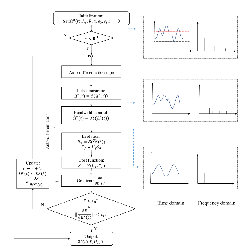
Figure 1: Flow diagram of COCOA. We use transform functions $\mathcal{C,M,E,F}$ to denote the 4 main nodes. Auto-differentiation tape is just a recorder that records all the computing processes automatically by Tensorflow and will be used for computing gradient. The figures on the left show the pulse’s change in time and frequency domain after each specific node.

The process of COCOA is shown as a flowchart in Fig. 1. The four main nodes in COCOA are pulse constraint, bandwidth control, evolution, and cost function. Pulse constraints and bandwidth control node are the core nodes, which always do a pretreatment on the pulse before evolution, while the form of evolution node and cost function node depend on the problem and optimization task. In the following, we elaborate each node and illustrate several unique features of CRAB.

III.3.1 Ansatz for pulses

The initial guess in COCOA can be chosen to be either a random guess or a specific form based on prior knowledge. Then it is transformed to an function for pulse parameters $\Omega_{j}(\vec{p},t)$, where $\vec{p}$ is the parameter vector. The analytical form of this function could be arbitrary according to the need in practice. For the consideration of limiting pulse bandwidth, without loss of generality, we take chopped Fourier basis functions as

$$\Omega_{j}(\vec{p},t)=a_{0}+\overset{N_{c}}{\underset{n=1}{\sum}}A_{jn}\cos(\omega_{jn}t)+B_{jn}\sin(\omega_{jn}t),$$ (3)

where pulse parameter set $\vec{p}$ is formed with Fourier expansion parameters

$$\vec{p}=\{A_{jn},B_{jn},a_{0}\}.$$ (4)

Analytical pulse functions solved from different theories could be exactly or approximately transformed to the chopped Fourier basis for optimization, such as Slepian pulses Martinis and Geller (2014), SWIPHT pulses Economou and Barnes (2015a); Deng et al. (2017), geometric pulses Deng et al. (2021), and so on. We will demonstrate this in Sec.IV.2.1. Note that filter functions for pulse pre-distortion could be directly applied on the Fourier basis, which brings additional convenience to experimental tune-ups.

In the PWC optimization, $\Omega_{j}(\vec{p},t)$ is discretized to a $N$-length sequence with sampling frequency $f_{s}=N/T$, where $T$ is the total gate time.

$$\Omega_{j}(\vec{p},t)\overset{\text{ sample }}{\longrightarrow}\{\Omega_{j}\left[\vec{p},k\right]\},k=1,\ldots,N.$$ (5)

For convenience, the discretized temporal sequence of the PWC ansatz is denoted as $\{\Omega_{j}[k]\},k=1,...,N$.

III.3.2 Amplitude constraint

A realistic system limits a maximal strength of the control field. Also, a single control pulse starts and ends at zero. As a traditional way in textbook  d’Alessandro (2007); Khaneja et al. (2005), this constraint enters the optimization cost function by adding up with the control power defined as $J=\lambda\int_{0}^{T}\Omega_{j}^{2}(t)dt$, where   the weight$\ \lambda>0$. However, the fidelity of optimized pulse will be lower with this term added. Furthermore, this way just gives a soft constraint on amplitude maximum, which could be harmful when physical systems have a hard limit on control amplitude. In our algorithm, a strong constraint to the pulse amplitude is added by passing the control pulses through a sigmoid window function, similar to GOAT Machnes et al. (2018).

$$S_{down}(t,g) =\frac{1}{1+e^{gt}}$$ (6)

$$S_{up}(t,g) =1-S_{down}(t,g)$$ (7)

$$S_{amp}(\Omega_{j}[k],l,u) =\left(2S_{up}\left(\frac{\Omega_{j}[k]-\frac{u+l}{2}}{\frac{u-l}{2}},0.5\right)-1\right)\frac{u-l}{2}$$

$$+\frac{u+l}{2},$$ (8)

where $g$ is the ascent/descent gradient of the window function. $l$, $u$ are the lower and upper bound of the pulse’s amplitude.

The total amplitude constraint transformation reads

$$\mathcal{C}(\Omega_{j}[k],t,l,u,g,\Delta_{t})$$

$$=S_{up}(\frac{t-\Delta t}{T},g)S_{down}(\frac{t-(T-\Delta t)}{T}),g)S_{amp}(\Omega_{j}[k],l,u),$$ (9)

where $\Delta t$ is the width of the ascent(descent) edge. The first and the second sigmoid function ensures zero amplitude at $t=0$ and $t=T$, and thus satisfies the second physical constraint. The last one bounds the amplitude to the $[l,u]$ range.

III.3.3 Bandwidth control

In this node, We modulate the control pulse to a bandwidth-limited one in frequency domain. Firstly, we transform the pulse sequence from time domain into frequency domain using discrete Fourier transform (DFT)

$$X[n]=\overset{N}{\underset{k=1}{\sum}}\Omega_{j}[k]e^{i(2\pi n/N)k}.$$ (10)

After DFT, We get a complex sequence $\{X[n]\},n=1,\ldots,N$. Assuming the upper cut-off frequency is $f_{th}$, we can derive the maximal Fourier component number $N_{c}$

$$N_{c}\leq\text{Int}(N\frac{f_{th}}{f_{s}})$$ (11)

where $\text{Int}(\cdot)$ indicates rounding down. Here, $N_{c}$ is a hyper-parameter in our algorithm and it affects the pulse’s simplicity, smoothness and numerical accuracy. We will discuss it in details in Sec. IV.

After DFT, the higher Fourier components over $N_{c}$, namely the complex sequence elements from $X[N_{c}+1]$ to $X[N-N_{c}]$ will be set to zero, i.e. limiting the bandwidth. Then the complex sequence in frequency domain becomes

$$Y[n]=\left\{\begin{array}[]{cll}\tilde{X}[n],&n\in[1,N_{c}]\cup[N-N_{c},N]&\\ 0,&n\in[N_{c}+1,N-N_{c}]&\end{array}\right.$$ (12)

Then we apply the inverse transformation of DFT, called IDFT, to transform the pulse back to time domain

$$\tilde{\Omega}_{j}[k]=\frac{1}{N}\overset{N}{\underset{n=1}{\sum}}Y[n]e^{i(2\pi k/N)n}.$$ (13)

After IDFT, the pulse sequence $\{\tilde{\Omega}_{j}[t_{k}]\}$ is a smooth pulse sequence with limited bandwidth. Its functional form in continuous time domain is denoted as

$$\tilde{\Omega}_{j}(t)=a_{0}+\sum_{n=1}^{N_{c}}A_{n}\cos(n\frac{2\pi f_{s}}{N}t+\phi_{n}).$$ (14)

It is worth noting that this is the functional form of our final optimized waveform, which is a finite Fourier basis function. More details about DFT and IDFT can be seen in appendix A.

III.3.4 Evolution

For the evolution node, the smooth, analytical and bandwidth-limited control pulse, Eq. (14), obtained from the previous nodes is taken into the dynamical equation to compute the time evolution. The choice of evolution equations, such as master equation and Schr$\ddot{o}$dinger equation, depends on the specific physical problem and optimization task. Here we consider a closed quantum system and use the PWC approach for the time evolution. Note that this could be upgraded to other finite difference methods to obtain more precise solution of the Schr$\ddot{o}$dinger equation. Here, the evolution operator at time $t_{k}$ reads

$$U_{k} =e^{-iH[t_{k}]\Delta t}$$

$$=e^{-i\left(H_{d}+{\underset{j}{\sum}}\tilde{\Omega}_{j}[t_{k}]H_{j}[t_{k}]\right)\Delta t}.$$ (15)

Then final evolution operator at time $t=T$ reads

$$U_{T}=U_{N}\ldots U_{1}U_{1}.$$ (16)

The final state $S_{T}$ reads

$$S_{T}=U_{T}S_{0}.$$ (17)

III.4 Pulse distortion in numerical process

There are at least three steps of pulse distortion in a complete quantum control task. First, the pulse distorted from the waveform optimized numerically because of the finite sampling rate of the arbitrary waveform generator (AWG) Lin et al. (2018); Raftery et al. (2017). Second, the pulse experience distortion during the transmission due to impedance mismatching and other realistic filtering effects Rol et al. (2020); Chen (2018); Baum et al. (2021); Hincks et al. (2015). Third, to force the optimized pulses satisfy physical constrains, pulse distortion is often induced when post-processing the output pulses from optimization iteration, such as adding filter functions to the output. As mentioned above, PWC algorithms, such as GRAPE and Krotov, generates rough pulses. In order to smoothen the optimal pulses, low-pass filter such as Gaussian filter  Ziegel (1988) could be applied to suppress or cut off the high frequency components and limit the bandwidth, after which the resultant waveform deforms and the fidelity is lowered from the optimum. On the other hand, limiting pulse amplitude Machnes et al. (2018) by applying a constraint function to the optimization results in distortion from the analytical form and induces additional high frequency components. However, COCOA introduce all the pulse constraints into the optimization before the DFT node and all the high frequency component will be filtered, overcoming this kind of pulse distortion perfectly. Additionally-customized constraints could be incorporated as well. This is enabled with the use of auto-differentiation in Tensorflow, which is discussed next. As a result, the optimized pulse is band-limited, maximum-limited, starting/ending at ZERO while a definite analytical waveform is guaranteed to output from the algorithm. This will be illustrated in Sec. IV

III.5 Auto-differentiation

Auto-differentiation (AD) method is widely used in machine learning, which is almost as accurate as symbolic differentiation Güneş Baydin et al. (2018). There are two points of necessity that we choose AD: (1) AD obtains the derivatives to all inputs in one back-propagation when AD works in the reverse mode. So it is much more efficient than manual and symbolic differentiation, and is more precise than numerical differentiation. (2) The complexity of derivatives induced by the bandwidth control and the extraction of computational subspace places much difficulties, such as expression swell problem, to manual and symbolic differentiation. The feasibility of auto-differentiation is demonstrated by the fact that each node of COCOA is derivable theoretically, so as the total transform function of inputs to cost function is $\mathbb{F}:\mathbb{R}^{n}\rightarrow\mathbb{R}$. This is suitable for the reverse mode of AD because the dimension of inputs is larger than outputs. We explicitly elaborate the process of auto-differentiation in COCOA optimization in Fig. 2. There are two processes when using auto-differentiation in reverse mode. i) Forward-propagation: when computing from $\{\Omega_{j}[k]\},k=1,...,N$ to $F$, it automatically constructs a computational graph formed of nodes and edges, as shown in Fig. 2 (solid line). ii) Back-propagation: The gradients of $F$ versus all inputs $\{\Omega_{j}[k]\},k=1,...,N$ are calculated with the computational graph by using chain rule, as shown in Fig. 2 (dashed line). We note that all the derivatives of $F$ with respect to inputs $\{\Omega_{j}[k]\},k=1,...,N$ are calculated in one back-propagation, which makes AD more efficient than other methods. Our numerical simulation results in Sec. IV will demonstrate the AD’s efficiency in quantum optimal control. For more details of AD, please refer to  Güneş Baydin et al. (2018).

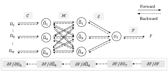
Figure 2: Computational graph of auto-differentiation. $\mathcal{C,M,E,F}$ denote four transform layers, corresponding to each node. ${\overline{\Omega}_{k}},{\widetilde{\Omega}_{k}},U_{T},F$ are the output sequence after each transform layer. The solid line(dashed line) is the forward propagation(backpropagation). Subscript $k$ denotes for the index of the control sequence $\Omega$. The dashed box at the bottom shows the process of computing the gradient of $F$ for $\Omega_{k}$, using the chain rule.

IV Applications on Superconducting Qubits

To demonstrate the advantage of COCOA, we apply this algorithm to tackle one of the most challenging control obstacles in the up-to-date multi-qubit processors: the always-on couplings. Such issue lies in many qubit systems such as superconducting qubits  Zhao et al. (2020); Ku et al. (2020); Deng et al. (2021), quantum dots Khaetskii et al. (2002); Jacak et al. (2013); Maksym and Chakraborty (1990), NMR qubits Vandersypen and Chuang (2005); Wang et al. (2016), etc. Scaling-up qubit systems tends to reduce the number of control degrees, which means taking out more control fields out of the system. Losing either the control of qubit frequencies or coupling strength brings more difficult in realizing good quantum gates, especially in the systems such as fixed frequency qubits with fixed couplings, tunable qubits with residual couplings, qubits with tunable couplings with unwanted interaction and crosstalk  Sarovar et al. (2020); Ash-Saki et al. (2020); Murali et al. (2020). Fortunately, the degree of control freedom on the pulse-shaping could be further exploited with the help of COCOA. In this section, without loss of generality, we consider two realistic models of multi-connected superconducting qubits and apply COCOA to find optimal control pulses for single-qubit and two-qubit gates for the always-coupled qubits.

IV.1 Model 1: Two transmon qubits coupled directly

In X-mon (X-shaped transmon) arrays where qubits are coupled directly via a capacitance with a constant interaction $g$, such as Google’s previous version of quantum computing chip Bristlecone Kelly et al. (2019) and other chip design with few control lines  Long et al. (2021). As a simplified model, we consider two qubit coupled directly and obtain the Hamiltonian as

$$H_{0}=\underset{j=1,2}{\sum}\omega_{j}a_{j}^{{\dagger}}a_{j}+\frac{\alpha_{j}}{2}a_{j}^{{\dagger}}a_{j}^{{\dagger}}a_{j}a_{j}+g_{12}(a_{1}^{{\dagger}}+a_{1})(a_{2}^{{\dagger}}+a_{2})$$ (18)

This model is effectively valid for qubits coupled via tunable couplers  Arute et al. (2019); Deng et al. (2021). Here $\omega_{j}$ are the qubit frequencies and $\alpha_{j}$ are the anharmonicities of transmon qubits, $j=1,2$. To implement single qubit operations, neighbour qubits are detuned with $\Delta=\omega_{1}-\omega_{2}$ and the effective zz-coupling strength is turned down with the rate $\frac{g_{12}^{2}}{\Delta}$ Deng et al. (2021); Krantz et al. (2019); Kjaergaard et al. (2020); Wendin (2017). $g_{12}$ is the capacitive coupling strength between two qubits. $a^{{\dagger}}(a)$ denotes the qubit creation (annihilation) operators. This unwanted coupling gives rise to frequency splitting between $\left|00\right\rangle\rightarrow\left|01\right\rangle$ and $\left|10\right\rangle\rightarrow\left|11\right\rangle$, inducing gate errors, as well as control crosstalk Deng et al. (2021). This could be a more challenging issue when qubit frequencies are fixed Long et al. (2021). Complex control pulses are proposed to resolved this issue but finding appropriate pulses remains a difficulty Deng et al. (2021); Khaneja et al. (2005). The microwave pulses are sent in to drive the transmons via this operator

$$H_{d}^{j}=a_{j}^{\dagger}e^{-i\omega_{d}t}+a_{j}e^{i\omega_{d}t}$$ (19)

where $\omega_{d}$ is the driving frequency. The waveform $\Omega(t)$ is applied to the drive and modulates the strength of the control pulse. Hence, the total Hamiltonian reads

$$H=H_{0}+\sum_{j}\Omega_{j}(t)H_{d}^{j}$$ (20)

The control field could be added to both qubit 1 and 2 simultaneously or only on a single qubit 1 or 2.

To illustrate the properties of COCOA’s solutions and demonstrate ths advantage of the algorithm, we show some numerical examples of optimizing quantum gates in realistic system by comparing different algorithms, including COCOA, CRAB, and GRAPE. For a fair comparison, we use gradient descent optimizer Adam Ruder (2016) in all these algorithms, but keep the rest steps the same as the original versions. Therefore, we denote them as COCOA, GRAPE-like and CRAB-like in our results. In the simulation, each transmon is truncated to a four-level system to better consider leakage. The model parameter we used is similar to Ref. Qiu et al. (2021) as $\omega_{1}/2\pi=5.270$ GHz, $\omega_{2}/2\pi=4.670$ GHz, $\alpha_{1}/2\pi=\alpha_{2}/2\pi=220$ MHz, $g_{12}/2\pi=25.4$ MHz. The initial pulses for all algorithms are identical and take the form as shown in Eq. (14).

Note that the coupling strength between the two qubit is at the order of $g/\omega\simeq 10^{-2}$. The results for the weak coupling $g/\omega\leq 10^{-3}$ and ultra-strong coupling regime $g/\omega\geq 10^{-1}$ are shown in appendix B, all of which demonstrating the enhancement of COCOA in the search of optimal pulses.

IV.1.1 Single qubit X gate at the presence of interaction

The first gate is a single X rotation only on the second qubit while remaining the state in the first qubit. The target evolution operator of the two qubit system is

$$U_{tar}=I\otimes\sigma_{x}$$ (21)

which include both qubit’s dynamics in the computational subspace $span\{\widetilde{\left|00\right\rangle},\widetilde{\left|01\right\rangle},\widetilde{\left|10\right\rangle},\widetilde{\left|11\right\rangle}\}$. The identity $I$ in the first qubit’s subsystem meets the requirement that the control field does net-zero operation to the first qubit at the presence of crosstalk due to the coupling. Applying simple pulses results in entanglement between this two qubits. However, COCOA can efficiently find composite pulses to achieve the $U_{tar}$ evolution. Here we set $\omega_{d}$ in resonance with transition $\widetilde{\left|00\right\rangle}\rightarrow\widetilde{\left|01\right\rangle}$, then it is off-resonant with $\widetilde{\left|10\right\rangle}\rightarrow\widetilde{\left|11\right\rangle}$  Deng et al. (2021). Other relevant parameters are $T=50$ns, $N=148$, $f_{s}/2\pi=N/T=2.96GHz$, $N_{c}=5$. The range of pulse amplitude is $[-30,30]$ MHz$\times 2\pi$.

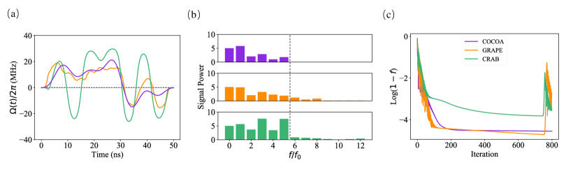
Figure 3: Algorithm comparison.(a) Optimized pulse with zero-point at $t=0$ ns and $t=50$ ns. Pulse amplitude is limited between $[-30,30]$ MHz. (b) Frequency spectrum of each pulse. $f_{0}=1/T=0.02$ GHz. As we can see that GRAPE(orange line) and CRAB(green line) have more high-frequency components induced by pulse constraints. The dashed line shows the truncated components of the COCOA algorithm. (c) Gate infidelity changing versus iteration, showing the efficiency of each algorithm.

We can conclude three advantages of COCOA according the comparison result in Fig. 3: (1) Accuracy. As shown in Fig. 3 (a), COCOA achieves the gate infidelity below $10^{-4}$, which is the same order of magnitude with GRAPE-like’s result and better than CRAB-like’s. Even better results could be obtained by enlarging $N_{c}$, as illustrated later in IV.1.3. (2) Smoothness and bandwidth. As shown in Fig. 3 (b), the optimal pulse obtained by COCOA shows the best smoothness and limited pulse amplitude within $[-20,20]$ MHz$\times 2\pi$. From the frequency spectrum of optimized pulse, as shown in Fig. 3 (c), COCOA has limited bandwidth but the other’s consist of high-frequency components. Interestingly, GRAPE-like’s pulse shows a similar profile as COCOA, with more high frequency components. Although CRAB-like’s pulse looks smooth too, its amplitude is significantly stronger than the other two. (3) Analyticity. As promised, COCOA gives a definite analytical summation form of the basis, all the high frequency components are filtered completely. Specifically, COCOA outputs the pulse parameters for Eq. (14) with

$$a_{0} =5.066$$

$$A_{1},\ldots,A_{5} =-11.66,-4.172,-5.753,2.140,3.497$$

$$\phi_{1},\ldots,\phi_{5} =1.080,-3.385,6.104,-1.458,1.098$$

GRAPE-like and CRAB-like both produce uncontrollable high frequency components and cannot obtain definite analytical expressions due to the ZERO starting and ending point constraint.

COCOA shows a great advantage here. Because the smoothness of control pulse is rather important in many qubit systems where leakage and crosstalk errors are significant. Limiting the bandwidth could also help reduce pulse distortion throughout all the control steps. Moreover, the analytical expression with definite summation of few chopped basis brings convenience and simplicity to the experimental adjustments. It is necessary to point out that, in principle, CRAB also uses analytical waveform with definite summation of chopped random basis, but the pulse constrains during optimization process induces numerical pulse distortion from the original analytical form, leading to higher frequency components, as shown in Fig. 3(c). Compared to GRAPE and CRAB, COCOA is so far the first algorithm producing definite analytical pulses.

IV.1.2 Dual X gate at the presence of interaction

Simultaneously driving coupled qubits is challenging task even in tunable qubit system where the interaction could be tuned on and off approximately. Crosstalk of control signals and zz-interaction cause significant drop of gate error compared to individual driving case. In order to implement a high fidelity dual (simultaneous) X gate on both nearest-coupled coupled qubits, we apply COCOA to find the pulses to drive them at the same time. The Dual X gate simultaneously flip the states of the first and second qubits. The target evolution operator of the two qubit system is

$$U_{tar}=\sigma_{x}\otimes\sigma_{x}$$ (22)

Both qubits should be driven simultaneously and the drive term follows the same form of Eq. 19. Hence, the total Hamiltonian reads

$$H=H_{0}+\Omega_{1}(t)H_{d}^{1}+\Omega_{2}(t)H_{d}^{2}$$ (23)

Here we use COCOA algorithm to find the optimized driving pulse of dual X gate and we set $T=50$ns$,N=200,N_{c}=5,f_{s}=N/T=4$ GHz. As we can see in Fig. 4, the optimized gate fidelity is greater than $99.9\%$ and the pulse parameter for each drive are given as following:

Pulse parameters for Q1:

$$a_{0} =5.091$$

$$A_{1},\ldots,A_{5} =-10.46,2.971,3.033,6.725,-6.124,$$

$$\phi_{1},\ldots,\phi_{5} =5.858,1.547,3.085,1.458,-3.650$$

Pulse parameter for Q2:

$$a_{0} =5.078$$

$$A_{1},\ldots,A_{5} =7.790,0.8855,4.857,-6.030,1.787$$

$$\phi_{1},\ldots,\phi_{5} =0.7156,1.714,2.507,0.8538,2.292$$

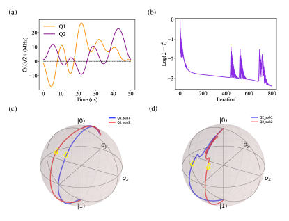
Figure 4: Dual X gate optimization using COCOA. (a) Optimized control pulse for each qubit with pulse amplitude limitation $[-30,30]$ MHz and ZERO starting and ending point. (b) Gate infidelity changes versus iteration, indicating the efficiency of the algorithm. (c) Evolution trajectories of qubit 1, driven by the darkorange pulse in (b). Blue(red) line shows the evolution in on-resonant (off-resonant) subspace span $\{\widetilde{\left|00\right\rangle},\widetilde{\left|01\right\rangle}\}$ ($\{\widetilde{\left|10\right\rangle},\widetilde{\left|11\right\rangle}\}$). (d) Evolution trajectories of qubit 2, driven by the purple pulse in (b). Blue and red line have the same meaning in (c)

By analyzing the driving pulse and its corresponding Bloch trajectory, we found that the negative part of the driving pulse eliminates the detuning of the off-resonance subspace with respect to on-resonance subspace, namely the zz-coupling.

IV.1.3 Optimizing $N_{c}$

The key parameter $N_{c}$, i.e. the number of Fourier components, determines the smoothness and bandwidth of the pulse, as well as the number of optimizing parameters, which increases at a scaling rate of $2N_{c}$. Consequently, the choice of $N_{c}$ affects the optimization efficiency and accuracy.

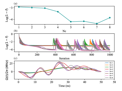
Figure 5: Explore how $N_{c}$ affects the accuracy, efficiency, and smoothness of our algorithm. (a) Best infidelity that COCOA can reach with each $N_{c}$. (b) Infidelity changes versus iterations for different $N_{c}$, indicating the efficiency. (c) Optimized pulse under different $N_{c}$.

We take the previous case in Sec. IV.1.1 as an example to study how $N_{c}$ affects the optimization, where we only tune $N_{c}$ while fixing all the other parameters. As shown in Fig. 5 (a), gate infidelity is improved by one order of magnitude when $N_{c}$ increases from $1$ to $5$, and doesn’t get much improved beyond $5$. Fig. 5 (b) and (c) demonstrate the convergence behavior and pulse shape of $N_{c}=1,2,...,8$. From these simulation results, we make an observation that $N_{c}=5$ is the best choice based on the consideration of the trade-off between number of parameters and optimization accuracy.

Theoretically, if there is no bandwidth limit, the COCOA algorithm can approach to GRAPE algorithm when $N_{c}$ reaches its maximum: $N_{c}^{max}=\text{Int}\left(\frac{N-1}{2}\right)$, where $\text{Int}(\cdot)$ means rounding down.

IV.2 Model 2: Two transmon qubits coupled via a Cavity

In another widely used architecture, superconducting qubits are coupled via superconducting cavities, such as one dimensional transmission line resonators Majer et al. (2007); Gong et al. (2019); Chow et al. (2012), with the Hamiltonian

$$H_{0}=\underset{j=1,2}{\sum}\omega_{j}a_{j}^{{\dagger}}a_{j}+\frac{\alpha_{j}}{2}a_{j}^{{\dagger}}a_{j}^{{\dagger}}a_{j}a_{j}+g_{cj}(b^{{\dagger}}a_{j}+ba_{j}^{{\dagger}})+\omega_{c}b^{{\dagger}}b$$ (24)

where $\omega_{c}$ are the frequency of the cavity. $g_{cj}$ is coupling strength between resonator and the $j$-th qubit. $b(b^{{\dagger}})$ is annihilation(creation) operator of resonator. Other parameters have the same meaning as in model 1. We take $\omega_{1}/2\pi=6.2$GHz, $\omega_{2}/2\pi=6.8$GHz, $\omega_{c}/2\pi=7.15$GHz, $\alpha_{1,2}/2\pi=350$MHz, $g_{1,2}/2\pi=250$MHz, which are used in Ref. Economou and Barnes (2015b). The drive Hamiltonian $H_{d}$ has the same form as Eq. 19.

Since the cavity behaves as merely a larger scale fixed-coupler between two qubits, control pulses for single-qubit gates could be obtained similarly as previous discussion. Detailed numerical results of single qubit X gate could be found in appendix C. Here we demonstrate an optimization of two-qubit entangling gate for this model.

IV.2.1 Optimizing CNOT gate based on SWIPHT protocal

It’s worth to point out that COCOA can fully utilize the prior knowledge of analytical methods and obtains completely analytical optimal pulses via local optimization around an analytically-given pulse. To demonstrate this, we start from a CNOT gate implementation using SWIPHT protocol (speeding up wave forms by inducing phases to harmful transitions) Economou and Barnes (2015b, a); Deng et al. (2017); Long et al. (2021). The given analytical form of the pulse is

$$\Omega(t)=\frac{\ddot{\chi}}{2\sqrt{\frac{\delta^{2}}{4}-\dot{\chi}^{2}}}-\sqrt{\frac{\delta^{2}}{4}-\dot{\chi}^{2}}\cot(2\chi)$$ (25)

where $\chi(t)=\frac{A}{T^{8}}t^{4}(T-t)^{4}+\frac{\pi}{4}$, $A=138.9$, $T=5.87/\left|\delta\right|$. $\delta=\omega_{\widetilde{10}\rightarrow\widetilde{11}}-\omega_{\widetilde{00}\rightarrow\widetilde{01}}$ is the detuning between the target and harmful transition in the computational subspace $span\{\widetilde{\left|01\right\rangle}$, $\widetilde{\left|01\right\rangle}$, $\widetilde{\left|10\right\rangle}$, $\widetilde{\left|11\right\rangle}\}$, where the first qubit is the control qubit and the second one is the target qubit.

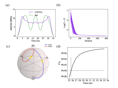
Figure 6: CNOT gate optimization using COCOA. (a) Pulse comparison between the initial SWIFT CNOT pulse (green-dashed line) in Ref.  Economou and Barnes (2015b) and our optimized CNOT pulse (purple-solid line). (b) Gate infidelity changes versus iteration, indicating the efficiency of the algorithm. (c) Evolution trajectory on Bloch sphere driven by our optimized pulse in (b). The blue and red lines show the target qubit’s evolution trajectory in the two subspaces $span\{\widetilde{\left|00\right\rangle},\widetilde{\left|01\right\rangle}\}\$and $span\{\widetilde{\left|10\right\rangle},\widetilde{\left|11\right\rangle}\}$. (d) The gate speed limit of CNOT.

The CNOT operator generated with a single microwave control could be expressed as this general form

$$U_{\text{tar }}=\left(\sigma_{x}\oplus I\right)\prod_{i=1,2;j=x,y,z}R_{ij}\left(\theta_{ij}\right)$$ (26)

where $R_{ij}(\theta_{ij})$ are single qubit rotations with arbitrary angles for optimization. This $U_{tar}$ is equivalent to a standard CNOT $\sigma_{x}\oplus I$ up to some local phases. We set drive frequency $\omega_{d}=\omega_{\widetilde{00}\rightarrow\widetilde{01}}$, and $N_{c}=9$. Fig. 6 (a) shows that the local optimization converges very fast with prior knowledge of optimal pulse, which demonstrates the advantage of numerical optimization based on analytically-optimal pulses. Fig. 6 (b) shows that the optimized CNOT pulses is transformed but still maintains similar shape as the initial analytically-optimal pulse. We note that the optimized pulse, show in Fig. 6 (b), can be generated more accurately with AWG device due to its limited bandwidth that the initial pulse doesn’t prosess. With the same evolution time $T=35.4$ ns, we finally obtained the optimized driving pulse shown in Fig. 6 (b) with complete pulse parameters (in the unit of MHz) in Eq. 14

$$a_{0} =7.416$$

$$A_{1},\ldots,A_{9} =-0.818,-2.05,-2.27,-1.50-0.807,$$

$$-0.2020.0287,0.325,0.00291$$

$$\phi_{1},\ldots,\phi_{9} =0,\pi,\pi,0,0,0,0.000138,0,0.00198$$

The speed of this analytical CNOT gate is limited by $\frac{\delta^{2}}{4}-\dot{\chi}^{2}>0$ derived from Eq. 25. Hence, $T>0.02975\frac{A}{\delta}$, and we have $T_{min}=24.95$ ns when $A=138$ and $\delta=26.4$ MHZ$\times 2\pi$. The behavior of the optimal CNOT gate approaching the speed limit is shown in Fig. 6 (c). Here, we start from $T=25$ ns and increase by $1$ ns each step to observe the change of the optimal fidelity with the gate time. Finally, we obtain the gate fidelity exceeds $99.9$% when $T\geqslant 26$ ns, which is a significantly improvement from the initial CNOT gate time 35 ns using SWIFT theory. Here we note two important tricks when using COCOA for a local optimization: 1. To obtain fast convergence in this local optimization scenario, see Fig. 6 (a), a small learning rate is favored, which is taken to be $0.001$; 2. The SGD optimizer is preferred to Adam optimizer, since Adam is more suitable for broader search range due to its momentum factor  Ruder (2016).

V Conclusion

In this paper, we have developed a novel algorithm to optimize smooth quantum control pulses constraints, which could be very complex, highly nonlinear, sub/super-differentiable approximations and optional. In the particular demonstration examples, we limit the pulse amplitude, pulse bandwidth, and the number of pulse parameters. Doing so makes this algorithm involve complicated computation for the differentiation of expectation function versus optimizing parameters. We resolve this issue using auto-differentiation powered by Tensorflow. Therefore, this algorithm can be straightforwardly extended to larger quantum systems with even more complicated calculations of gradients. We have demonstrated the advantages of the proposed algorithm by applying it to realistic superconducting qubit models with always-on ZZ-interaction, and achieve optimal smooth pulses to implement single-qubit gates and two-qubit gates. Comparing to GRAPE and CRAB algorithms, we obtain higher gate fidelities and better optimization efficiency. We have shown that COCOA could be applied to the optimization scenarios either with or without good prior knowledge by simply switching the optimizers, and obtain high-fidelity gates for both cases.

We summarize COCOA’s advantages as follows: 1. COCOA outputs optimal pulses with definite analytical expression. 2. The optimal pulses have manually limited bandwidth and amplitude. 3. This algorithm is more compatible with complex and flexible pulse constraints, without the induced pulse distortion in numerical optimization. 4. The auto-differentiation assisted by Tensorflow enables efficient and easy calculation of gradients and the ability to handle complex computing processes and complex models. 5. COCOA can speed up the optimization by locally searching the optimal pulses based on certain prior knowledge. Using COCOA, we completely resolve the challenging problem, to implement either individually or simultaneously a single qubit X-gate in a strongly ZZ-interacting two-qubit system Long et al. (2021); Deng et al. (2021); Ash-Saki et al. (2020). In conclusion, COCOA optimization is friendly to realistic quantum control tasks, easy to be customized, and easy to be extended to larger quantum systems.

In conclusion, COCOA provides a versatile, highly functional and efficient platform to add physical constraints into quantum optimal control tasks. Following the line of COCOA, more work could be pursued in a near future to resolve the realistic QOC issues. For example, pulse pre-distortion could be effectively performed by adding the definite transfer function of control lines and pulse generators into optimization process; Different analytical forms with fewer pulse parameters could be investigated using the proposed algorithm, so that the numerical approach could better meet the experimental needs.

Author contributions

YS and XHD conceived the project, designed the algorithm, performed calculations, and wrote the manuscript. YS did all the coding. JL gave some important suggestions on the algorithm and help design the flowchart. YJH helped with refining the algorithm. QG assisted with GRAPE optimization. XHD oversaw the project.

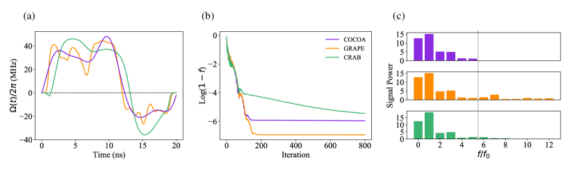
Figure 7: Algorithm comparison. $g=1$MHz$\times 2\pi$. (a) Optimized pulse with zero-point at $t=0$ ns and $t=20$ ns. Pulse amplitude is limited between $[-40,40]$ MHz.(b) Gate infidelity changing versus iteration, showing the efficiency of each algorithm. (c) Frequency spectrum of each pulse. $f_{0}=1/T=0.05$ GHz. As we can see that GRAPE(orange line) and CRAB(green line) have more high-frequency components induced by pulse constraints. The dashed line shows the truncated components of COCOA algorithm.

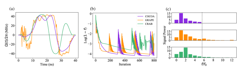
Figure 8: Algorithm comparison. $g=100$MHz$\times 2\pi$ (a) Optimized pulse with zero-point at $t=0$ns and $t=20$ns. The pulse amplitude is limited between $[-40,40]$ MHz. (b) Gate infidelity changing versus iteration, showing the efficiency of each algorithm. (c) Frequency spectrum of each pulse. $f_{0}=1/T=0.025$ GHz. As we can see that GRAPE (orange line) and CRAB (green line) have more high-frequency components induced by pulse constraints. The dashed line shows the truncated components of COCOA algorithm.

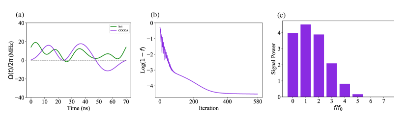
Figure 9: Single X gate for model 2. (a) Optimized pulse with zero-point at $t=0$ ns and $t=70$ ns. Pulse amplitude is limited between $[-20,20]$ (unit:MHz). The purple line is the optimized pulse with COCOA algorithm and the green line is the initial Fourier pulse. (b) Gate infidelity changing versus iteration, showing the efficiency of the algorithm. (c) Frequency spectrum of COCOA pulse with limited-bandwidth($N_{c}=5$). $f_{0}=\frac{1}{T}=0.0143$GHz.

Appendix A Low Pass Filtering

DFT: Given a discretized pulse sequence in time domain $\Omega_{j}[k],k=1\ldots N$. Note that the pulse here can be any form or without any form. After DFT we can get a complex sequence which contains amplitude and phase information.

$$X[n]=\overset{N}{\underset{k=1}{\sum}}\Omega_{j}[k]e^{i(2\pi n/N)k}.$$ (27)

We can deduce that

$$X[N-n] =\sum_{k=1}^{N}\Omega_{j}[k]e^{-j(2\pi/N)(N-n)k}$$ (28)

$$=\sum_{k=1}^{N}\Omega_{j}[k]e^{j(-2k\pi+(2\pi/N)kn)}$$ (29)

$$=\sum_{k=1}^{N}\Omega_{j}[k]e^{j((2\pi/N)kn)}$$ (30)

$$=X^{*}[n].$$ (31)

This is an important characteristic of the complex sequence.

IDFT:

$$\tilde{\Omega}_{j}[k]=\frac{1}{N}\overset{N}{\underset{n=1}{\sum}}Y[n]e^{i(2\pi k/N)n}.$$ (32)

Assuming $N$ is oven number, We can deduce that

$$N\times\Omega_{j}[k] =\sum_{n=1}^{N}X[n]e^{j(2\pi/N)kn}$$ (33)

$$=X[0]+X[1]e^{j(2n\pi/N)}+X[2]e^{j(2(2n\pi/N))}+\cdots$$

$$+X[N/2-1]e^{j\left(\frac{2n\pi}{N}(N/2-1)\right)}+X[N/2]$$

$$+X[N/2+1]e^{j\left(\frac{2n\pi}{N}(N/2+1)\right)}+\cdots$$

$$+X[N-2]e^{j\left(\frac{2n\pi}{N}(N-2)\right)}+X[N-1]e^{j\left(\frac{2n\pi}{N}(N-1)\right)}.$$ (34)

We set $X[n]=a_{n}+ib_{n}$. Considering sum of term $X[n]$ and $X[N-n]$, by utilizing the conjugate property, we can deduce

$$\left(a_{n}+jb_{n}\right)e^{j(2\pi/N)kn}+\left(a_{n}-jb_{k}\right)e^{j(2\pi/N)\left(N-k\right)n}$$

$$=A_{n}\cos\left(\frac{2kn\pi}{N}+\phi_{n}\right)$$ (35)

where $A_{n}=2\sqrt{a_{n}^{2}+b_{n}^{2}}$ and $\tan\left(\phi_{n}\right)=\frac{b_{n}}{a_{n}}$. Then the total expression of $\Omega_{j}[k]$ in time domain reads

$$N\times\Omega_{j}[k] =a_{0}+A_{1}\cos(n2\pi/N+\phi_{1})$$

$$+A_{2}\cos((2n)2\pi/N+\phi_{2})+\cdots$$

$$+A_{\frac{N}{2}-1}\cos\left(((N/2-1)n)2\pi/N+\phi_{\frac{N}{2}-1}\right).$$ (36)

Assume sample frequency is $f_{s}$ we have

$$\Omega_{j}[k]=\Omega_{j}[kT_{s}]=\Omega_{j}(k/f_{s}).$$ (37)

Replace $k$ with $f_{s}t$

$$N\times\Omega_{j}(t) =a_{0}+A_{1}\cos(f_{s}2\pi t/N+\phi_{1})$$

$$+A_{2}\cos((2f_{s})2\pi t/N+\phi_{2})+\cdots$$

$$+A_{\frac{N}{2}-1}\cos\left(((N/2-1)f_{s})2\pi t/N+\phi_{\frac{N}{2}-1}\right).$$ (38)

And we can deduce the frequency at $k_{c}$ is $2\pi k_{c}f_{s}/N=2\pi f$.

Appendix B Weak and strong coupling strength

This appendix demonstrates that COCOA algorithm can still be efficient in different coupling strength. In Fig. 7, we show the algorithm comparison with $g=0.001$GHz$\times 2\pi$. Fig. 8 shows the result of $g=0.1$GHz$\times 2\pi$

Appendix C single qubit X gate with always on interaction for Model 2

Here we show the result of single qubit X gate in Model 2 using COCOA algorithm to show its power and compatibility to multi-qubit system. The result is show in Fig. 9.

References

- Steane (1998) A. Steane, Reports on Progress in Physics 61, 117 (1998).
- Degen et al. (2017) C. L. Degen, F. Reinhard, and P. Cappellaro, Reviews of modern physics 89, 035002 (2017).
- Giovannetti et al. (2011) V. Giovannetti, S. Lloyd, and L. Maccone, Nature photonics 5, 222 (2011).
- Naranjo et al. (2018) T. Naranjo, K. M. Lemishko, S. de Lorenzo, Á. Somoza, F. Ritort, E. M. Pérez, and B. Ibarra, Nature communications 9, 1 (2018).
- Basset et al. (2021) F. B. Basset, F. Salusti, L. Schweickert, M. B. Rota, D. Tedeschi, S. C. da Silva, E. Roccia, V. Zwiller, K. D. Jöns, A. Rastelli, et al., npj Quantum Information 7, 1 (2021).
- Rembold et al. (2020) P. Rembold, N. Oshnik, M. M. Müller, S. Montangero, T. Calarco, and E. Neu, AVS Quantum Science 2, 024701 (2020).
- Chen et al. (2021) Z. Chen, K. J. Satzinger, J. Atalaya, A. N. Korotkov, A. Dunsworth, D. Sank, C. Quintana, M. McEwen, R. Barends, P. V. Klimov, et al., arXiv preprint arXiv:2102.06132 (2021).
- Motzoi et al. (2009) F. Motzoi, J. M. Gambetta, P. Rebentrost, and F. K. Wilhelm, Physical review letters 103, 110501 (2009).
- Economou and Barnes (2015a) S. E. Economou and E. Barnes, Physical Review B 91, 161405 (2015a).
- Deng et al. (2017) X.-H. Deng, E. Barnes, and S. E. Economou, Physical Review B 96, 035441 (2017).
- Doria et al. (2011) P. Doria, T. Calarco, and S. Montangero, Physical review letters 106, 190501 (2011).
- Deng et al. (2021) X.-H. Deng, Y.-J. Hai, J.-N. Li, and Y. Song, arXiv preprint arXiv:2103.08169 (2021).
- Long et al. (2021) J. Long, T. Zhao, M. Bal, R. Zhao, G. S. Barron, H.-s. Ku, J. A. Howard, X. Wu, C. R. H. McRae, X.-H. Deng, et al., arXiv preprint arXiv:2103.12305 (2021).
- Machnes et al. (2018) S. Machnes, E. Assémat, D. Tannor, and F. K. Wilhelm, Physical review letters 120, 150401 (2018).
- Khaneja et al. (2005) N. Khaneja, T. Reiss, C. Kehlet, T. Schulte-Herbrüggen, and S. J. Glaser, Journal of magnetic resonance 172, 296 (2005).
- Machnes et al. (2011) S. Machnes, U. Sander, S. J. Glaser, P. de Fouquieres, A. Gruslys, S. Schirmer, and T. Schulte-Herbrüggen, Physical Review A 84, 022305 (2011).
- Ruschhaupt et al. (2012) A. Ruschhaupt, X. Chen, D. Alonso, and J. Muga, New Journal of Physics 14, 093040 (2012).
- Zahedinejad et al. (2014) E. Zahedinejad, S. Schirmer, and B. C. Sanders, Physical Review A 90, 032310 (2014).
- Caneva et al. (2011) T. Caneva, T. Calarco, and S. Montangero, Physical Review A 84, 022326 (2011).
- Ohtsuki et al. (2004) Y. Ohtsuki, G. Turinici, and H. Rabitz, The Journal of chemical physics 120, 5509 (2004).
- Lloyd and Montangero (2014) S. Lloyd and S. Montangero, Physical review letters 113, 010502 (2014).
- Ohtsuki and Nakagami (2008) Y. Ohtsuki and K. Nakagami, Physical Review A 77, 033414 (2008).
- Sundermann and de Vivie-Riedle (1999) K. Sundermann and R. de Vivie-Riedle, The Journal of chemical physics 110, 1896 (1999).
- Jerger et al. (2019) M. Jerger, A. Kulikov, Z. Vasselin, and A. Fedorov, Physical review letters 123, 150501 (2019).
- Hincks et al. (2015) I. Hincks, C. Granade, T. W. Borneman, and D. G. Cory, Physical Review Applied 4, 024012 (2015).
- Rol et al. (2020) M. A. Rol, L. Ciorciaro, F. K. Malinowski, B. M. Tarasinski, R. E. Sagastizabal, C. C. Bultink, Y. Salathe, N. Haandbæk, J. Sedivy, and L. DiCarlo, Applied Physics Letters 116, 054001 (2020).
- Tošner et al. (2009) Z. Tošner, T. Vosegaard, C. Kehlet, N. Khaneja, S. J. Glaser, and N. C. Nielsen, Journal of Magnetic Resonance 197, 120 (2009).
- Jones (2010) J. A. Jones, arXiv preprint arXiv:1011.1382 (2010).
- Ryan et al. (2009) C. Ryan, M. Laforest, and R. Laflamme, New Journal of Physics 11, 013034 (2009).
- Nielsen et al. (2007) N. C. Nielsen, C. Kehlet, S. J. Glaser, and N. Khaneja, eMagRes (2007).
- Schutjens et al. (2013) R. Schutjens, F. A. Dagga, D. Egger, and F. Wilhelm, Physical Review A 88, 052330 (2013).
- Blais et al. (2020a) A. Blais, S. M. Girvin, and W. D. Oliver, Nature Physics 16, 247 (2020a).
- Allen et al. (2017) J. L. Allen, R. Kosut, J. Joo, P. Leek, and E. Ginossar, Physical Review A 95, 042325 (2017).
- Blais et al. (2007) A. Blais, J. Gambetta, A. Wallraff, D. I. Schuster, S. M. Girvin, M. H. Devoret, and R. J. Schoelkopf, Physical Review A 75, 032329 (2007).
- Blais et al. (2020b) A. Blais, A. L. Grimsmo, S. Girvin, and A. Wallraff, arXiv preprint arXiv:2005.12667 (2020b).
- Niemeyer (2013) I. O. Niemeyer (2013).
- Wang and Dobrovitski (2011) Z.-H. Wang and V. Dobrovitski, Physical Review B 84, 045303 (2011).
- Platzer et al. (2010) F. Platzer, F. Mintert, and A. Buchleitner, Physical review letters 105, 020501 (2010).
- van Frank et al. (2016) S. van Frank, M. Bonneau, J. Schmiedmayer, S. Hild, C. Gross, M. Cheneau, I. Bloch, T. Pichler, A. Negretti, T. Calarco, et al., Scientific reports 6, 1 (2016).
- Niu et al. (2019a) M. Y. Niu, S. Boixo, V. N. Smelyanskiy, and H. Neven, npj Quantum Information 5, 1 (2019a).
- Shu et al. (2016a) C.-C. Shu, T.-S. Ho, X. Xing, and H. Rabitz, Physical Review A 93, 033417 (2016a).
- Niu et al. (2019b) M. Y. Niu, S. Boixo, V. N. Smelyanskiy, and H. Neven, npj Quantum Information 5, 1 (2019b).
- Kirchhoff et al. (2018) S. Kirchhoff, T. Keßler, P. J. Liebermann, E. Assémat, S. Machnes, F. Motzoi, and F. K. Wilhelm, Physical Review A 97, 042348 (2018).
- Larocca and Wisniacki (2020) M. Larocca and D. Wisniacki, arXiv preprint arXiv:2010.03598 (2020).
- Plick and Krenn (2015) W. N. Plick and M. Krenn, Physical Review A 92, 063841 (2015).
- Moore and Rabitz (2012) K. W. Moore and H. Rabitz, The Journal of chemical physics 137, 134113 (2012).
- Kelly et al. (2014) J. Kelly, R. Barends, B. Campbell, Y. Chen, Z. Chen, B. Chiaro, A. Dunsworth, A. G. Fowler, I.-C. Hoi, E. Jeffrey, et al., Physical review letters 112, 240504 (2014).
- Rol et al. (2019) M. Rol, F. Battistel, F. Malinowski, C. Bultink, B. Tarasinski, R. Vollmer, N. Haider, N. Muthusubramanian, A. Bruno, B. Terhal, et al., arXiv preprint arXiv:1903.02492 (2019).
- Abadi et al. (2016) M. Abadi, A. Agarwal, P. Barham, E. Brevdo, Z. Chen, C. Citro, G. S. Corrado, A. Davis, J. Dean, M. Devin, et al., arXiv preprint arXiv:1603.04467 (2016).
- Shu et al. (2016b) C.-C. Shu, T.-S. Ho, X. Xing, and H. Rabitz, Physical Review A 93, 033417 (2016b).
- Pedersen et al. (2007) L. H. Pedersen, N. M. Møller, and K. Mølmer, Physics Letters A 367, 47 (2007).
- Rabiner and Gold (1975) L. R. Rabiner and B. Gold, Englewood Cliffs: Prentice-Hall (1975).
- Chen (2018) Z. Chen, Metrology of quantum control and measurement in superconducting qubits (University of California, Santa Barbara, 2018).
- Martinis and Geller (2014) J. M. Martinis and M. R. Geller, Physical Review A 90, 022307 (2014).
- d’Alessandro (2007) D. d’Alessandro, Introduction to quantum control and dynamics (CRC press, 2007).
- Lin et al. (2018) J. Lin, F.-T. Liang, Y. Xu, L.-H. Sun, C. Guo, S.-K. Liao, and C.-Z. Peng, arXiv preprint arXiv:1806.03660 (2018).
- Raftery et al. (2017) J. Raftery, A. Vrajitoarea, G. Zhang, Z. Leng, S. Srinivasan, and A. Houck, arXiv preprint arXiv:1703.00942 (2017).
- Baum et al. (2021) Y. Baum, M. Amico, S. Howell, M. Hush, M. Liuzzi, P. Mundada, T. Merkh, A. R. Carvalho, and M. J. Biercuk, arXiv preprint arXiv:2105.01079 (2021).
- Ziegel (1988) E. R. Ziegel, Filtering in the time and frequency domains (1988).
- Güneş Baydin et al. (2018) A. Güneş Baydin, B. A. Pearlmutter, A. Andreyevich Radul, and J. Mark Siskind, Journal of Machine Learning Research 18, 1 (2018), ISSN 15337928, eprint 1502.05767.
- Zhao et al. (2020) P. Zhao, P. Xu, D. Lan, J. Chu, X. Tan, H. Yu, and Y. Yu, Physical Review Letters 125, 200503 (2020).
- Ku et al. (2020) J. Ku, X. Xu, M. Brink, D. C. McKay, J. B. Hertzberg, M. H. Ansari, and B. Plourde, Physical review letters 125, 200504 (2020).
- Khaetskii et al. (2002) A. V. Khaetskii, D. Loss, and L. Glazman, Physical review letters 88, 186802 (2002).
- Jacak et al. (2013) L. Jacak, P. Hawrylak, and A. Wojs, Quantum dots (Springer Science & Business Media, 2013).
- Maksym and Chakraborty (1990) P. Maksym and T. Chakraborty, Physical review letters 65, 108 (1990).
- Vandersypen and Chuang (2005) L. M. Vandersypen and I. L. Chuang, Reviews of modern physics 76, 1037 (2005).
- Wang et al. (2016) Y. Wang, A. Kumar, T.-Y. Wu, and D. S. Weiss, Science 352, 1562 (2016).
- Sarovar et al. (2020) M. Sarovar, T. Proctor, K. Rudinger, K. Young, E. Nielsen, and R. Blume-Kohout, Quantum 4, 321 (2020).
- Ash-Saki et al. (2020) A. Ash-Saki, M. Alam, and S. Ghosh, IEEE Transactions on Quantum Engineering 1, 1 (2020).
- Murali et al. (2020) P. Murali, D. C. McKay, M. Martonosi, and A. Javadi-Abhari, in Proceedings of the Twenty-Fifth International Conference on Architectural Support for Programming Languages and Operating Systems (2020), pp. 1001–1016.
- Kelly et al. (2019) J. Kelly, Z. Chen, B. Chiaro, B. Foxen, J. Martinis, and Q. H. T. Team, in APS March Meeting Abstracts (2019), vol. 2019, pp. A42–002.
- Arute et al. (2019) F. Arute, K. Arya, R. Babbush, D. Bacon, J. C. Bardin, R. Barends, R. Biswas, S. Boixo, F. G. Brandao, D. A. Buell, et al., Nature 574, 505 (2019).
- Krantz et al. (2019) P. Krantz, M. Kjaergaard, F. Yan, T. P. Orlando, S. Gustavsson, and W. D. Oliver, Applied Physics Reviews 6, 021318 (2019).
- Kjaergaard et al. (2020) M. Kjaergaard, M. E. Schwartz, J. Braumüller, P. Krantz, J. I.-J. Wang, S. Gustavsson, and W. D. Oliver, Annual Review of Condensed Matter Physics 11, 369 (2020).
- Wendin (2017) G. Wendin, Reports on Progress in Physics 80, 106001 (2017).
- Ruder (2016) S. Ruder, arXiv preprint arXiv:1609.04747 (2016).
- Qiu et al. (2021) J. Qiu, Y. Zhou, C.-K. Hu, J. Yuan, L. Zhang, J. Chu, W. Huang, W. Liu, K. Luo, Z. Ni, et al., arXiv preprint arXiv:2104.02669 (2021).
- Majer et al. (2007) J. Majer, J. Chow, J. Gambetta, J. Koch, B. Johnson, J. Schreier, L. Frunzio, D. Schuster, A. A. Houck, A. Wallraff, et al., Nature 449, 443 (2007).
- Gong et al. (2019) M. Gong, M.-C. Chen, Y. Zheng, S. Wang, C. Zha, H. Deng, Z. Yan, H. Rong, Y. Wu, S. Li, et al., Physical review letters 122, 110501 (2019).
- Chow et al. (2012) J. M. Chow, J. M. Gambetta, A. D. Corcoles, S. T. Merkel, J. A. Smolin, C. Rigetti, S. Poletto, G. A. Keefe, M. B. Rothwell, J. R. Rozen, et al., Physical review letters 109, 060501 (2012).
- Economou and Barnes (2015b) S. E. Economou and E. Barnes, Physical Review B 91, 161405(R) (2015b).