AMRA*: Anytime Multi-Resolution Multi-Heuristic A*

Abstract

Heuristic search-based motion planning algorithms typically discretise the search space in order to solve the shortest path problem. Their performance is closely related to this discretisation. A fine discretisation allows for better approximations of the continuous search space, but makes the search for a solution more computationally costly. A coarser resolution might allow the algorithms to find solutions quickly at the expense of quality. For large state spaces, it can be beneficial to search for solutions across multiple resolutions even though defining the discretisations is challenging. The recently proposed algorithm Multi-Resolution A* (MRA*) searches over multiple resolutions. It traverses large areas of obstacle-free space and escapes local minima at a coarse resolution. It can also navigate so-called narrow passageways at a finer resolution. In this work, we develop AMRA*, an anytime version of MRA*. AMRA* tries to find a solution quickly using the coarse resolution as much as possible. It then refines the solution by relying on the fine resolution to discover better paths that may not have been available at the coarse resolution. In addition to being anytime, AMRA* can also leverage information sharing between multiple heuristics. We prove that AMRA* is complete and optimal (in-the-limit of time) with respect to the finest resolution. We show its performance on 2D grid navigation and 4D kinodynamic planning problems.

I Introduction

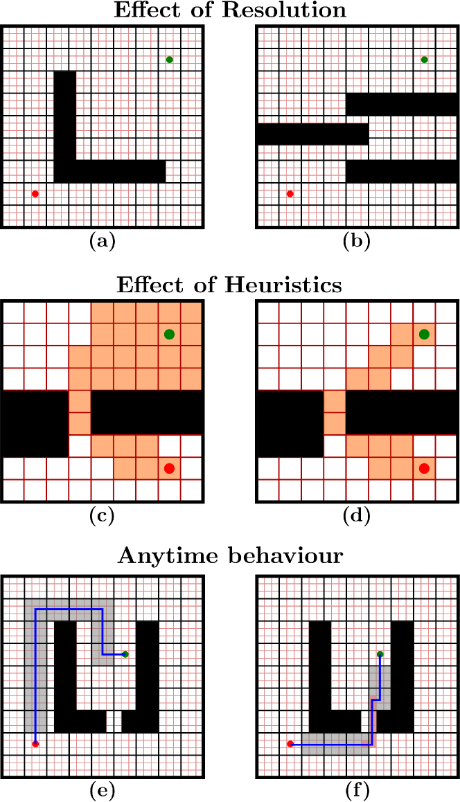
Figure 1: Effect of Resolution: local minima can be explored quicker at coarser resolutions (a), while finer resolutions help navigate through narrow passageways (b); Effect of Heuristics: a less informed heuristic (c) expands many more states than an informed heuristic (d); and Anytime behaviour: an initial suboptimal solution (e) can be improved over time (f). The pictures show start states in green, goal states in red.

Heuristic search algorithms for robot motion planning find least-cost solutions in discretised approximations of the continuous state space of the robot. They have shown impressive results in robot manipulation [1], navigation [2], task planning [3], and multi-robot coordination [4]. The size of the search space for these algorithms is determined by the dimensionality of the robot state space and, crucially, the discretisation level of each of these dimensions [5]. If the state space is discretised finely the search needs to explore a greater number of possible robot states in order to find a solution which is computationally costly. However at the same time, this higher resolution allows the search to find potential solutions through narrow passageways and dense obstacle clutter. A coarse discretisation of the state space is useful in relatively obstacle-free areas of the environment, and for the search to escape local minima where the heuristic estimate of the cost-to-goal is weakly correlated with the true cost-to-goal. The downside is that the search might fail to find a solution at that resolution.

At the same time, it is important for heuristic search algorithms to be instantiated with useful heuristics as they determine the computational effort spent exploring areas of the search space to find a solution. If a heuristic estimate of the cost-to-goal is poorly correlated with the true cost-to-goal, search algorithms can spend a lot of time expanding states in these local minima before finding a path to goal [6]. Multi-heuristic search algorithms [7] were developed to alleviate this problem by allowing search algorithms to be instantiated with multiple heuristics. These are not only easier to define for the practitioner, but also allow for information sharing between heuristics to better guide the search.

In this work we present AMRA*, an Anytime Multi-Heuristic Multi-Resolution A* search algorithm that is capable of searching a state space at multiple levels of discretisation, share information between multiple heuristics, and improve the quality of the solution found over time. It is able to determine the appropriate resolution for exploring local minima and navigating across obstacle-free space and narrow passageways. It takes advantage of different heuristics being better correlated with the true cost-to-goal in different regions of the search space. Finally, with every iteration of the search loop, AMRA* is able to improve its solution with tighter suboptimality bounds and find the optimal solution in-the-limit of time.

Fig. 1 shows simple examples of three aspects of heuristic search that AMRA* encapsulates in one general algorithm while maintaining important theoretical properties of completeness and (sub-)optimality. First, in Fig. 1 (a), if we follow a greedy heuristic to the goal, the obstacle introduces a local minima with many more states at the fine resolution (light red grid) than the coarse resolution (black grid). In this case, running a search at coarse resolution will find a path to the goal with less computation. The downside of using only a coarse resolution is shown in Fig. 1 (b), where a solution only exists at the fine resolution. Fig. 1 (c-d) show the effect of using a less informed heuristic (Euclidean distance) vis-a-vis a perfect heuristic (backward Dijkstra search from the goal). For more complicated problems, different heuristics can be informative in different regions of the state space, and a search algorithm that can take advantage of this can greatly improve performance. Finally, an anytime algorithm like AMRA* relies heavily on the coarse resolution to quickly find an initial solution in Fig. 1 (e) (coarse states are highlighted in gray). It goes on to improve this solution over time to also include fine resolution states (highlighted in light red) in Fig. 1 (f).

II Related Work

AMRA* is an anytime, multi-heuristic, multi-resolution search algorithm for solving robot motion planning problems. It builds on the family of best-first search algorithms that traces its roots back to classic A* and Weighted A* (wA*) search algorithms [8, 9]. For a large class of real-world robotics applications, optimal motion planning can be intractable due to the expansive nature of robot state spaces. Anytime algorithms allow us to solve problems in these domains by finding an initial highly suboptimal solution quickly, and spending any remaining planning budget to improve that solution. ARA* [10] is an anytime version of wA* and provides bounds on solution suboptimality that Anytime A* [11] does not. van den Berg et. al [12] present ANA*, a non-paramateric version of ARA* .

While anytime algorithms have the ability to refine solutions over time, their performance is determined by the heuristic. The use of multiple heuristics within a search algorithm can dramatically improve search performance since different heuristics can offer better guidance in different regions of state space [13, 7]. Recently, Natarajan et. al. [14] have also developed an anytime multi-heuristic algorithm.

Contemporaneous to the development of anytime and multi-heuristic algorithms, there has been work on developing algorithms that utilise multiple levels of discretisation of the robot state space. These multi-resolution algorithms rely on a coarser discretisation to navigate large regions of obstacle-free space, and revert to a finer discretisation to maneuver through narrow passageways [15, 16, 17].

Most of the algorithms discussed above have provable bounds on solution suboptimality. Some sampling-based planners for robot motion planning [18] offer a different notion of solution optimality. They are asymptotically optimal, and thus will find the optimal solution given infinite time. As such, they can be interrupted early to exhibit an anytime behaviour.

We compare the performance of AMRA* in this paper with the three most closely related heuristic search algorithms (ARA* [10], MRA* [17] and A-MHA* [14]) and against an asymptotically optimal sampling-based algorithm (RRT* [18]).

III Problem Formulation

We define a robot motion planning problem with the tuple $(\mathcal{X},x_{s},\mathcal{G})$, where $\mathcal{X}$ is the state space of the robot, $x_{s}\in\mathcal{X}$ is the start state, and $\mathcal{G}\subset\mathcal{X}$ is a set of goal states. $\mathcal{X}_{\text{free}}\subset\mathcal{X}$ denotes the obstacle-free space in the environment. A solution to the motion planning problem, if one exists, is a collision-free path from $x_{s}$ to $\mathcal{G}$.

We assume access to a cost function $c:\mathcal{X}\times\mathcal{X}\rightarrow\mathbb{R}_{\geq 0}$ to compute the cost of an action between two robot states. The cost of a potential solution path $\pi=\{x_{1},\ldots,x_{n}\}$ is denoted by overloading the definition of cost function $c$ as $c(\pi)=\sum_{i=1}^{N-1}c(x_{i},x_{i+1})$. Our goal in this paper is to solve the least-cost path planning problem and find the optimal path $\pi^{*}=\operatorname*{arg\,min}_{\pi}c(\pi)$.

IV Graph Construction and Search

We solve the least-cost robot motion planning problem with a heuristic search algorithm over a graph $G=(V,E)$. The vertex set $V\subset\mathcal{X}$ contains robot states. Edges $e=(x_{i},x_{j})\in E$ connect two vertices $x_{i},x_{j}\in V$ if the robot can execute an action that takes it from $x_{i}$ to $x_{j}$. Thus each edge $e\in E$ is also an action $a$ in the robot action space $\mathcal{A}$.

IV-A Action Spaces

AMRA* constructs its vertex set $V=\bigcup_{r}V_{r}$ as a union over different levels of discretisation or resolutions $r$ of $\mathcal{X}$. Each vertex set $V_{r}$ has a corresponding edge set $E_{r}$ which make up the edges $E=\bigcup_{r}E_{r}$ used by AMRA* when constructing $G$. We represent each edge set $E_{r}$ with an action space $\mathcal{A}_{r}$ available to the robot. The core underlying assumption in this work and robot motion planning with multiple resolutions in general is that for every resolution $r$ being used, the robot has access to actions $\mathcal{A}_{r}$ that take it between two states $x_{u},x_{v}\in V_{r}$. Note that this formulation allows for a state $x\in\mathcal{X}$ to exist at multiple resolutions $r$, and thus in multiple vertex and edge sets $V_{r},E_{r}$.

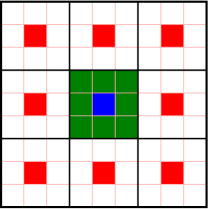
Figure 2: Multi-resolution action space for 8-connected grid navigation. The robot (at the blue state) can execute fine resolution actions to green states, and coarse resolution actions to red states.

Fig. 2 shows an example of a multi-resolution action space for 2D grid navigation. AMRA* does not require that coarse actions be made up of fine actions, nor does it require any action to end in states that exist at multiple resolutions. However as we discuss in Section IV-B, especially for multi-heuristic search, it can be useful to construct action spaces that lead to significant overlap between vertex sets at different resolutions.

IV-B Multi-Heuristic Search

A heuristic function $h:V\rightarrow\mathbb{R}_{\geq 0}$ is an estimate of the cost-to-goal from a state $x\in V$ on the graph $G$. Heuristics are admissible if they under-estimate the true cost-to-goal from $x$ to $\mathcal{G}$ on $G$. AMRA* executes a multi-heuristic search derived from MHA* [7] which allows the use of multiple inadmissible heuristics. AMRA* parameterises heuristics by the resolution $r$ for which they are applicable. The search is initialised with a set of heuristics, at least one per resolution $r$ used. The MHA* framework allows us to use any number of additional heuristics for each resolution.

As with MHA* and MRA*, it is necessary to initialise AMRA* with an anchor heuristic which is consistent, i.e. a heuristic function $h$ such that $h(x_{i})\leq h(x_{j})+c(x_{i},x_{j})\forall e=(x_{i},x_{j})\in E$. We reserve the resolution $r=0$ to refer to this anchor search. The anchor search uses the full action space of the robot $\mathcal{A}_{0}=\bigcup_{r>0}\mathcal{A}_{r}$ to construct the graph $G_{0}=(V_{0},E_{0})$. This implies $V_{0}=\bigcup_{r>0}V_{r}$, and we refer to the anchor search vertex set as the union space. If all coarse resolution states coincide with some state at the finest resolution ($V_{r}\subset V_{1}\,\forall\,r>1$), this is easily achieved by running the anchor search at the finest resolution ($V_{0}\equiv V_{1}$).

Using multiple heuristics at the same resolution allows us to share information between these heuristics by maintaining a single cost-to-come value (cost of the current best path between the start and some state) and multiple cost-to-goal estimates for a state. This information sharing allows the search to potentially escape local minima for some heuristic in a region of the state space on the basis of guidance from another heuristic at that resolution in that region.

V Algorithm

Algorithm 1 AMRA*

1:procedure Key($x,i$)

2:    return $g(x)+w_{1}\times h_{i}(x)$

3:procedure Expand($x,i$)

4:    $r\leftarrow\texttt{Res}(i)$

5:    if $i\neq 0$ then

6:         for all $j>0$ do $\triangleright$ Loop over search queues

7:             if $j\neq i\wedge\texttt{Res}(j)==r$ then

8:                 Remove $x$ from $OPEN_{j}$                           

9:    for $x^{\prime}\in\texttt{Succs}(x,\mathcal{A}_{r})$ do

10:         if $g(x^{\prime})>g(x)+c(x,x^{\prime})$ then

11:             $g(x^{\prime})\leftarrow g(x)+c(x,x^{\prime})$

12:             $bp(x^{\prime})\leftarrow x$

13:             if $x^{\prime}\in CLOSED_{0}$ then

14:                 $\texttt{Insert}(x^{\prime},INCONS)$

15:             else

16:                 $\texttt{Update}(x^{\prime},OPEN_{0},\textsc{Key}(x^{\prime},0)$

17:                 for all $j\in\{1,\ldots,M\}$ do

18:                     $l\leftarrow\texttt{Res}(j)$

19:                     if $l\notin\texttt{Resolutions}(x^{\prime})$ then

20:                         continue                      

21:                     if $x^{\prime}\notin CLOSED_{l}$ then

22:                         if $\textsc{Key}(x^{\prime},j)\leq w_{2}\times\textsc{Key}(x^{\prime},0)$ then

23:                             $\texttt{Update}(x^{\prime},OPEN_{j},\textsc{Key}(x^{\prime},j))$                                                                                          

24:procedure ImprovePath( )

25:    while $OPEN_{i}$ is not empty $\forall i\in\{0,\ldots M\}$ do

26:         $i\leftarrow\texttt{ChooseQueue}()$ $\triangleright$ over inadmissible queues

27:         if $OPEN_{i}.\text{min}()\leq w_{2}\times OPEN_{0}.\text{min}()$ then

28:             $x\leftarrow OPEN_{i}.\text{top}()$ $\triangleright$ $OPEN_{i}.\text{top}()$ also pops

29:             $\textsc{Expand}(x,i)$

30:             $r\leftarrow\texttt{Res}(i)$

31:             $\texttt{Insert}(x,CLOSED_{r})$

32:             if $x\in\mathcal{G}$ then

33:                 $x_{\text{goal}}\leftarrow x$

34:                 return true              

35:         else

36:             $x\leftarrow OPEN_{0}.\text{top}()$

37:             $\textsc{Expand}(x,0)$

38:             $\texttt{Insert}(x,CLOSED_{0})$

39:             if $x\in\mathcal{G}$ then

40:                 $x_{\text{goal}}\leftarrow x$

41:                 return true                           

42:procedure Main($x_{s},\mathcal{G},\{\mathcal{A}_{r}\}_{r=0}^{N},\{h_{i}\}_{i=0}^{M},w_{1}^{\text{init}},w_{2}^{\text{init}}$)

43:    $w_{1}\leftarrow w_{1}^{\text{init}},w_{2}\leftarrow w_{2}^{\text{init}}$

44:    $g(x_{s})=0$

45:    $bp(x_{s})\leftarrow NULL$

46:    for all $i\in\{0,\ldots,M\}$ do

47:         $OPEN_{i}.\text{clear}()$ $\triangleright$ Initialise priority queues     

48:    $\texttt{Insert}(x_{s},INCONS)$

49:    while $w_{1}\geq 1\,\wedge\,w_{2}\geq 1$ do

50:         for all $x\in INCONS$ do

51:             $\texttt{Update}\left(x,OPEN_{0},\textsc{Key}(x,0)\right)$          

52:         $INCONS.\text{clear}()$

53:         for all $x\in OPEN_{0}$ do

54:             for all $j\in\{1,\ldots,M\}$ do

55:                 if $\texttt{Res}(j)\in\texttt{Resolutions}(x)$ then

56:                     $\texttt{Update}\left(x,OPEN_{j},\textsc{Key}(x,j)\right)$                                        

57:         for all $r\in\{0,\ldots,N\}$ do

58:             $CLOSED_{r}.\text{clear}()$          

59:         if $\textsc{ImprovePath}()$ then

60:             Publish current solution by tracing $bp(x_{\text{goal}})$ till $x_{s}$          

61:         if $w_{1}==1\,\wedge\,w_{2}==1$ then

62:             break          

63:         Update $w_{1},w_{2}$     

Algorithm 1 contains the full AMRA* search procedure. AMRA* is initialised with the start state $x_{s}$, goal set $\mathcal{G}$, action spaces $\{\mathcal{A}_{0},\ldots,\mathcal{A}_{N}\}$, and heuristics $\{h_{0},\ldots,h_{M}\}$. The state space $\mathcal{X}$ is discretised into $N$ levels. For $i<j$, resolution $i$ is finer than resolution $j$. The anchor action space is the union action space ($\mathcal{A}_{0}=\bigcup_{r=1}^{N}\mathcal{A}_{r}$), and the anchor search is run at the finest resolution ($V_{0}\equiv V_{1}$). The anchor heuristic $h_{0}$ is consistent (and thus admissible), while the other heuristics may be inadmissible. There is at least one heuristic per resolution, thus $M\geq N$.

V-A Connections to Existing Algorithms

AMRA* is a generalisation of several existing search algorithms. With a single heuristic per resolution, if we do not run AMRA* anytime, AMRA* is the same as MRA* [17]. We can also run AMRA* for a single resolution, with multiple heuristics at that resolution, and obtain either A-MHA* [14] or MHA* [7] depending on whether it is run anytime or not. In slightly more contrived scenarios, for a single resolution and a single heuristic, AMRA* can also devolve to ARA* [10] and Weighted A* (wA*) [9]. The connections stem from the fact that AMRA* utilises multiple resolutions, multiple heuristics, and is anytime.

V-B AMRA* Desiderata

We denote the cost-to-come for a state with the function $g:V\rightarrow\mathbb{R}_{\geq 0}$. The parent of a state $x$, denoted by $bp(x)$ is its predecessor on the best known path from $x_{s}$ to $x$. Resolutions$(x)$ returns the set of resolutions state $x$ lies on: $r\in\texttt{Resolutions}(x)\Rightarrow x\in V_{r}$. Each resolution $r$ is associated with a container for states expanded at that resolution, $CLOSED_{r}$. Res$(i)$ returns the resolution associated with heuristic $h_{i}$. Each heuristic $h_{i}$ is associated with a priority queue $OPEN_{i}$. Succs$(x,\mathcal{A}_{r})$ generates all valid successors of $x$ at resolution $r$ using the appropriate action space $\mathcal{A}_{r}$. For $r=0$, this generates all valid successors of $x$ for all resolutions in Resolutions$(x)$.

V-C Algorithmic Details

The anytime nature of AMRA* is controlled by the loop in Line 49. The suboptimality of the solution is controlled by parameters $w_{1},w_{2}$. At the end of each iteration, AMRA* returns a solution which is at most $w_{1}\times w_{2}$ suboptimal with respect to the graph $G_{0}=(V_{0},E_{0})$ (from Theorem 3). $w_{1},w_{2}$ are decreased in Line 63 in order to potentially improve the solution quality in the next iteration. To facilitate this, AMRA* maintains $INCONS$ - a container for all inconsistent states. These are states whose cost-to-come, or $g$-value, is improved after they have been expanded from the admissible anchor search. If a state becomes inconsistent, a better solution through it might be found than the current best known solution. Hence these states are added back into the appropriate $OPEN_{i}$ for consideration by the search (Lines 50 and 53).

ImprovePath is the core function that searches for a path between $x_{s}$ and $\mathcal{G}$. $x_{\text{goal}}\in\mathcal{G}$ is some state which satisfies the termination condition in Line 32 or Line 39. If no such $x_{\text{goal}}$ is found before all $OPEN_{i}$ are exhausted (Line 25), AMRA* terminates with failure. Line 26 controls the scheduling policy over all heuristics. While many options exist [19], for AMRA* we use a simple round robin.

The core modification in AMRA* over MRA* and MHA* is the way in which the graph is constructed in Expand. Any time a state is expanded at a particular resolution, it is removed from all inadmissible (non-anchor) heuristics at that resolution (in the loop in Line 6). This is because the $g$-value of an inadmissibly expanded state is independent of the heuristic it was expanded from. The Expand function generates the successors of state $x$ by using the appropriate action space $\mathcal{A}_{r}$ (Line 9). After checking for successor consistency in Line 13, a newly generated state is inserted at all appropriate resolutions (Lines 16 to 23).

VI Theoretical Analysis

Theorem 1

AMRA* expands each state at most $N+1$ times per iteration.

Proof:

Any state that is expanded must be in some $OPEN_{i}$ (Lines 28 and 36). Upon admissible expansion from the anchor search, the state is inserted into $CLOSED_{0}$ (Line 38) and never inserted into $OPEN_{0}$ again (Line 13). For inadmissible expansions, the state is removed from all $OPEN_{i}$ for the appropriate resolution $r$ in the loop in Line 6, and inserted into $CLOSED_{r}$ in Line 31. This can happen once per resolution. Thus a state can be expanded at most $N+1$ times per iteration of AMRA*. ∎

Theorem 2

AMRA* is complete with respect to the graph $G_{0}=(V_{0},E_{0})$.

Proof:

AMRA* can either terminate after finding a solution in Line 34 or 41, or without a solution after exhausting all $OPEN_{i}$ and exiting the loop in Line 25. Since $\mathcal{A}_{0}=\bigcup_{r>0}\mathcal{A}_{r}$ and any edge $e\in E_{0}$ is an action $a\in\mathcal{A}_{0}$, $V_{0}=\bigcup_{r>0}V_{r}$. A consequence of this is that any solution at any resolution $r\geq 0$ must exist in $G_{0}$. Furthermore, if AMRA* exits the loop in Line 25, no states in $V_{0}$ remain to be expanded. Thus, AMRA* terminates in failure iff there is no solution in the graph $G_{0}$. ∎

Theorem 3

At the end of each iteration AMRA* returns a solution, if one exists, that is at most $w_{1}\times w_{2}$ suboptimal with respect to the optimal solution in graph $G_{0}=(V_{0},E_{0})$.

Proof:

(Sketch) AMRA* is complete with respect to $G_{0}$ (from Theorem 2). The anchor search is a wA* search with a consistent heuristic and suboptimality factor $w_{1}$. Thus if AMRA* terminates via the anchor search in Line 41, $g(x_{\text{goal}})\leq w_{1}\times g^{*}(x_{\text{goal}})$ (from [20]). If AMRA* terminates via an inadmissible heuristic in Line 34, $g(x_{\text{goal}})\leq w_{2}\times OPEN_{0}.\text{min}()\leq w_{2}\times w_{1}\times g^{*}(x_{\text{goal}})$ (from [7]). Thus any solution returned by AMRA* is at most $w_{1}\times w_{2}$ suboptimal with respect to $G_{0}$. ∎

VII Experimental Results

VII-A Illustrative Example

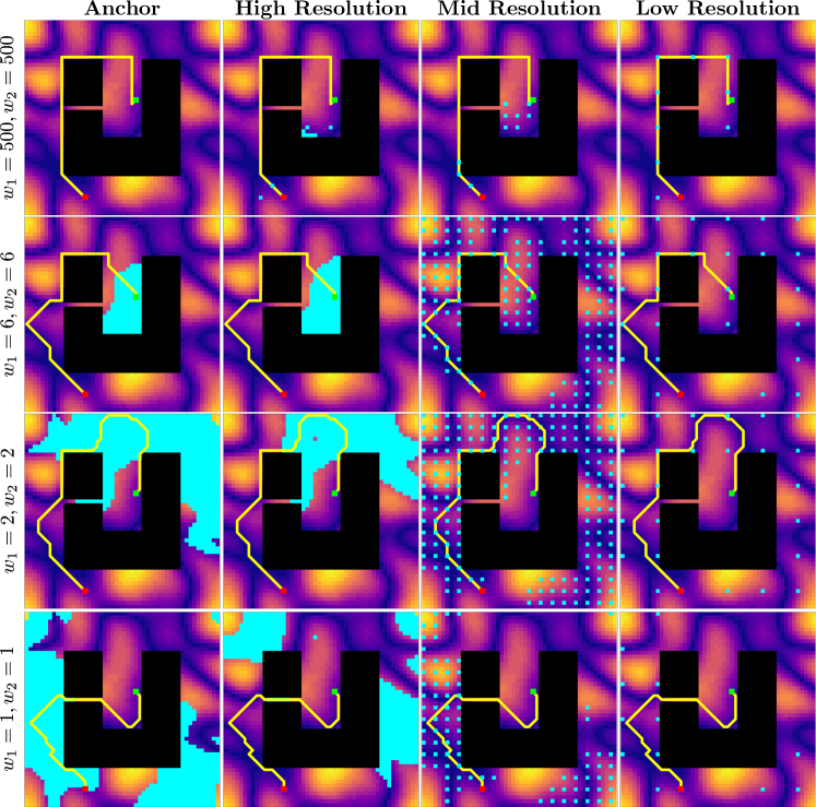
Figure 3: AMRA* execution on a 2D grid map with non-uniform costs. Start state (inside cul-de-sac) is in green, goal state in red, states expanded in cyan, and solution path in yellow. Each row is one iteration within AMRA*, and each column shows expansions from different state space discretisations. Cell costs increase from purple to orange. Best viewed in colour.

Fig. 3 shows a 2D grid navigation example to illustrate the behaviour showed by AMRA*. We run AMRA* on a $50\times 50$ map with three levels of discretisation: high ($1\times 1$), mid ($3\times 3$), and low ($9\times 9$). Each $1\times 1$ cell in the map has an assigned cost in the range $[10,260]$. The robot can execute actions on an 8-connected grid at all resolutions, and the cost of an action is the sum of costs of $1\times 1$ cells along that action. Only a single Euclidean distance heuristic was used. After finding an initial solution mostly at the low resolution, AMRA* expands more states at the finer resolutions over subsequent iterations to improve solution quality and finally terminates with the optimal solution for $w_{1}=1,w_{2}=1$.

VII-B 2D Grid Navigation

TABLE I: 2D Grid Navigation Results

	AMRA*		MRA*		ARA* (High)		ARA* (Mid)		ARA* (Low)		RRT*
Metrics	Cauldron (M1)	TheFrozenSea (M2)	M1	M2	M1	M2	M1	M2	M1	M2	M1	M2
Success $\%$	100	100	100	100	100	100	98	99	20	30	100	100
$T_{i}($\mathrm{ms}$)$	1.2 $\pm$ 0.98	1.08 $\pm$ 1.04	1.03$\times$	1.01$\times$	11.27$\times$	13.63$\times$	0.73$\mathbf{\times}$	0.49$\times$	0.27$\times$	0.32$\mathbf{\times}$	158.84$\times$	256.85$\times$
$T_{f}($\mathrm{ms}$)$	280.39 $\pm$ 302.88	223.81 $\pm$ 280.36	1.4$\times$	1.37$\times$	1.13$\times$	1.46$\times$	0.07$\mathbf{\times}$	0.04$\mathbf{\times}$	0.07$\times$	0.05$\times$	53.88$\times$	30.36$\times$
$c_{i}$	1163.06 $\pm$ 574.31	953.14 $\pm$ 480.8	1$\times$	1$\times$	1.02$\times$	1.01$\times$	1$\times$	0.98$\times$	1.19$\times$	1.38$\times$	0.74$\mathbf{\times}$	0.81$\mathbf{\times}$
$c_{f}$	902.12 $\pm$ 403.27	754.7 $\pm$ 367.75	1$\times$	1$\times$	1$\times$	1$\times$	1.06$\times$	1.03$\times$	1.32$\times$	1.61$\times$	0.86$\mathbf{\times}$	0.85$\mathbf{\times}$
$\lvert V_{0}\lvert\,(\times 10^{4})$	11.87 $\pm$ 11.63	9.51 $\pm$ 11.44	1.57$\times$	1.5$\times$	2.17$\times$	2.66$\times$	0.1$\mathbf{\times}$	0.1$\mathbf{\times}$	0.12$\times$	0.1$\mathbf{\times}$	6.1$\times$	1.71$\times$

We test the performance of AMRA* for a 2D grid navigation task on two $1024\times 1024$ maps from the MovingAI benchmark [21] shown in Fig. 4. The state space was discretised at three levels: high ($1\times 1$), mid ($7\times 7$), and low ($21\times 21$). A four-connected action space was used at each resolution and a single Manhattan distance heuristic was used. For each map, 100 random start and goal states were sampled at the low resolution. In this experiment, we compare the multi-resolution and anytime behaviour of AMRA* against MRA* and also ARA* run at each of the three resolutions denoted as “ARA* (High)”, “ARA* (Mid)” and “ARA* (Low)”. Since MRA* is not anytime, we ran a succession of MRA* searches with the same schedule of suboptimality weights as AMRA*. Additionally, we compare against an asymptotically optimal sampling-based planner RRT* [18] from OMPL [22].

Table I presents the result of these experiments. We report six metrics: success rate, times to initial and final solutions ($T_{i}$ and $T_{f}$ respectively, in milliseconds), costs of initial and final solutions ($c_{i}$ and $c_{f}$ respectively), and the number of state expansions $\lvert V_{0}\lvert$. All planners were given a $5$\mathrm{s}$$ timeout. We report raw numbers for AMRA* and relative numbers for the other algorithms, averaged over the 100 trials.

AMRA* is faster than the complete search-based baselines (MRA* and ARA* (High)) and expands fewer states, while converging to the optimal solution. The convergence behaviour of these algorithms is shown in Fig. 5. AMRA* is also much faster than RRT* , albeit finding costlier solutions on a discretised grid representation of the environment.

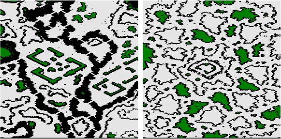
Figure 4: The four Starcraft maps from the MovingAI benchmark used for 2D grid navigation experiments: Cauldron (left) and TheFrozenSea (right). Green and black areas are obstacles.

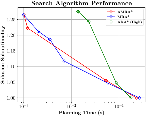
Figure 5: Performance of search algorithms on TheFrozenSea map from Fig. 4. Data was averaged over 100 runs. The x-axis is in log scale. MRA* was run iteratively as described in Sec. VII-B.

VII-C UAV Navigation

TABLE II: 2D Grid Navigation Results

	AMRA*		MRA* (E)		MRA* (Dubins)		MRA* (Dijkstra)		A-MHA* (High)
Metrics	Boston (M1)	NewYork (M2)	M1	M2	M1	M2	M1	M2	M1	M2
$T_{i}($\mathrm{s}$)$	0.31 $\pm$ 0.25	0.26 $\pm$ 0.23	0.69$\times$	1.4$\times$	1.11$\times$	0.33$\times$	1.01$\mathbf{\times}$	1.04$\times$	0.94$\times$	0.94$\mathbf{\times}$
$T_{f}($\mathrm{s}$)$	10.46 $\pm$ 10.77	9.54 $\pm$ 10.65	1.9$\times$	1.97$\times$	3.4$\times$	3.46$\times$	0.74$\mathbf{\times}$	0.75$\mathbf{\times}$	12.32$\times$	19.89$\times$
$c_{i}$	135.64 $\pm$ 66.15	109.48 $\pm$ 49.52	1.12$\times$	1.06$\times$	1.36$\times$	1.37$\times$	1.04$\times$	0.98$\times$	1.86$\times$	2.07$\times$
$c_{f}$	105.34 $\pm$ 46.61	92.47 $\pm$ 39.46	1$\times$	1$\times$	1$\times$	1$\times$	1$\times$	1$\times$	2.23$\times$	2.35$\times$
$\lvert V_{0}\lvert\,(\times 10^{5})$	1.74 $\pm$ 1.9	1.56 $\pm$ 1.87	1.27$\times$	1.4$\times$	4.84$\times$	4.15$\times$	0.82$\mathbf{\times}$	0.83$\mathbf{\times}$	20.59$\times$	42.99$\mathbf{\times}$
Timeout $\%$	15	12	39	29	30	23	6	4	74	82

The second set of experiments studies the multi-heuristic capabilities of AMRA* in addition to the multi-resolution and anytime behaviour. We solve kinodynamic motion planning problems for a 4D UAV robot modeled with double integrator dynamics. The state space of the robot is $(x,y,\theta,v)$ - its 2D pose in $SE(2)$ and linear velocity. The motion primitives used for the search algorithms are shown in Fig. 6. They exist at two resolutions for the 2D position: $3$\mathrm{m}$$ (high) and $9$\mathrm{m}$$ (low). The heading $\theta$ can take 12 discrete values in $[0,2\pi)$, and the velocity $v$ can be $\{0,3,8\}$\mathrm{m}\text{\,}{\mathrm{s}}^{-1}$$ at the end of a primitive. The cost of an action is its duration, thus we are solving for the least-time path in this experiment.

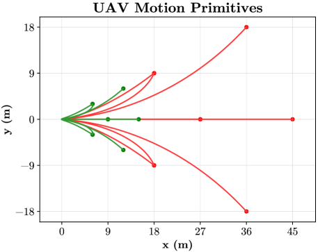
Figure 6: Motion primitives for UAV navigation. High resolution primitives are in green, and low resolution primitives are in red.

We use three inadmissible heuristics for this experiment: Euclidean distance to the goal (always used as the admissible anchor heuristic as well), Dubins path [23] distance to the goal, and a backwards Dijkstra search from the goal. AMRA* uses all three heuristics at both resolutions. 100 random start and goal states were sampled in two maps shown in Fig. 7 at the low resolution, and planners were given a timeout of $30$\mathrm{s}$$. We compare against two search-based algorithms: MRA* and A-MHA*. The former is not a multi-heuristic algorithm, thus we compare against instantiations which use different heuristics: “MRA* (E)”, “MRA* (Dubins)”, and “MRA* (Dijkstra)”. We also compare against “A-MHA* (High)” since that is not a multi-resolution algorithm. “A-MHA* (Low)” was unable to find any solutions across the $2\times 100$ problems.

Table II shows the results of these experiments. As in Section VII-B, we present raw numbers for AMRA* and relative numbers for the other baselines, averaged over 100 trials. Since all these algorithms succeeded in finding an initial solution, we report the timeout percentage (percentage of problems that reached the planning timeout before finding the final solution) in place of success rate. Overall, AMRA* is the most consistent algorithm when compared against the baselines. It finds the optimal solution much faster than “MRA* (E)”, “MRA* (Dubins)”, and “A-MHA* (High)” and with fewer timeouts. In most cases it is also quicker to find the first solution than all MRA* variants. “MRA* (Dijkstra)” is the most competitive baseline as it finds the optimal solution quicker, with fewer expansions and fewer timeouts. This comparison shows the effect of the overhead of AMRA* using multiple heuristics and multiple resolutions.

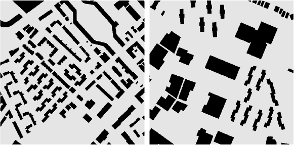
Figure 7: The two city/street maps from the MovingAI benchmark used for UAV navigation experiments: Boston_0_1024 (left) and NewYork_0_1024 right. Given the fixed discretisations for $\theta$ and $v$, there are roughly $2.8\times 10^{7}$ valid states in these maps.

VIII Discussion & Future Work

In this work we present AMRA* an anytime, multi-resolution, multi-heuristic search algorithm that generalises several existing search algorithms into one unified algorithm. It it very flexible for robot motion planning problems that have previously benefited from anytime algorithms, multiple heuristics, and multiple resolutions in separate lines of research. AMRA* exhibits impressive performance on two very different planning domains in 2D grid navigation and 4D kinodynamic UAV planning.

AMRA* at its core utilises multiple action spaces. Plenty of robotic systems are capable of a diverse set of actions that may dynamically become available to the robot given the state it is in. For example, a robot arm might plan in free space with simple motor primitives (independent joint angle changes), but might need to resort to prehensile and non-prehensile interaction actions in the vicinity of clutter. AMRA* opens the door for developing search algorithms that reason about such dynamically evolving action spaces that include both robot-centric and object-centric actions.

References

- [1] B. J. Cohen, S. Chitta, and M. Likhachev, “Single- and dual-arm motion planning with heuristic search,” Int. J. Robotics Res., vol. 33, no. 2, pp. 305–320, 2014. [Online]. Available: https://doi.org/10.1177/0278364913507983
- [2] S. Liu, K. Mohta, N. Atanasov, and V. Kumar, “Search-based motion planning for aggressive flight in SE(3),” IEEE Robotics Autom. Lett., vol. 3, no. 3, pp. 2439–2446, 2018. [Online]. Available: https://doi.org/10.1109/LRA.2018.2795654
- [3] C. R. Garrett, T. Lozano-Pérez, and L. P. Kaelbling, “FFRob: An efficient heuristic for task and motion planning,” in Algorithmic Foundations of Robotics XI - Selected Contributions of the Eleventh International Workshop on the Algorithmic Foundations of Robotics, WAFR 2014, 3-5 August 2014, Boğaziçi University, İstanbul, Turkey, ser. Springer Tracts in Advanced Robotics, H. L. Akin, N. M. Amato, V. Isler, and A. F. van der Stappen, Eds., vol. 107. Springer, 2014, pp. 179–195. [Online]. Available: https://doi.org/10.1007/978-3-319-16595-0_11
- [4] G. Wagner and H. Choset, “M*: A complete multirobot path planning algorithm with performance bounds,” in 2011 IEEE/RSJ International Conference on Intelligent Robots and Systems, IROS 2011, San Francisco, CA, USA, September 25-30, 2011. IEEE, 2011, pp. 3260–3267. [Online]. Available: https://doi.org/10.1109/IROS.2011.6095022
- [5] S. M. LaValle, Planning Algorithms. Cambridge University Press, 2006. [Online]. Available: http://planning.cs.uiuc.edu/
- [6] J. Hoffmann, “Local search topology in planning benchmarks: An empirical analysis,” in Proceedings of the Seventeenth International Joint Conference on Artificial Intelligence, IJCAI 2001, Seattle, Washington, USA, August 4-10, 2001, B. Nebel, Ed. Morgan Kaufmann, 2001, pp. 453–458.
- [7] S. Aine, S. Swaminathan, V. Narayanan, V. Hwang, and M. Likhachev, “Multi-Heuristic A*,” Int. J. Robotics Res., vol. 35, no. 1-3, pp. 224–243, 2016. [Online]. Available: https://doi.org/10.1177/0278364915594029
- [8] P. E. Hart, N. J. Nilsson, and B. Raphael, “A formal basis for the heuristic determination of minimum cost paths,” IEEE Trans. Syst. Sci. Cybern., vol. 4, no. 2, pp. 100–107, 1968. [Online]. Available: https://doi.org/10.1109/TSSC.1968.300136
- [9] I. Pohl, “Heuristic search viewed as path finding in a graph,” Artif. Intell., vol. 1, no. 3, pp. 193–204, 1970. [Online]. Available: https://doi.org/10.1016/0004-3702(70)90007-X
- [10] M. Likhachev, G. J. Gordon, and S. Thrun, “ARA*: Anytime A* with provable bounds on sub-optimality,” in Advances in Neural Information Processing Systems 16 [Neural Information Processing Systems, NIPS 2003, December 8-13, 2003, Vancouver and Whistler, British Columbia, Canada], S. Thrun, L. K. Saul, and B. Schölkopf, Eds. MIT Press, 2003, pp. 767–774. [Online]. Available: https://proceedings.neurips.cc/paper/2003/hash/ee8fe9093fbbb687bef15a38facc44d2-Abstract.html
- [11] R. Zhou and E. A. Hansen, “Multiple sequence alignment using anytime A*,” in Proceedings of the Eighteenth National Conference on Artificial Intelligence and Fourteenth Conference on Innovative Applications of Artificial Intelligence, July 28 - August 1, 2002, Edmonton, Alberta, Canada, R. Dechter, M. J. Kearns, and R. S. Sutton, Eds. AAAI Press / The MIT Press, 2002, pp. 975–977. [Online]. Available: http://www.aaai.org/Library/AAAI/2002/aaai02-155.php
- [12] J. van den Berg, R. Shah, A. Huang, and K. Y. Goldberg, “Anytime Nonparametric A*,” in Proceedings of the Twenty-Fifth AAAI Conference on Artificial Intelligence, AAAI 2011, San Francisco, California, USA, August 7-11, 2011, W. Burgard and D. Roth, Eds. AAAI Press, 2011. [Online]. Available: http://www.aaai.org/ocs/index.php/AAAI/AAAI11/paper/view/3680
- [13] M. Helmert, “The fast downward planning system,” J. Artif. Intell. Res., vol. 26, pp. 191–246, 2006. [Online]. Available: https://doi.org/10.1613/jair.1705
- [14] R. Natarajan, M. S. Saleem, S. Aine, M. Likhachev, and H. Choset, “A-MHA*: Anytime multi-heuristic A*,” in Proceedings of the Twelfth International Symposium on Combinatorial Search, SOCS 2019, Napa, California, 16-17 July 2019, P. Surynek and W. Yeoh, Eds. AAAI Press, 2019, pp. 192–193. [Online]. Available: https://aaai.org/ocs/index.php/SOCS/SOCS19/paper/view/18383
- [15] A. W. Moore and C. G. Atkeson, “The parti-game algorithm for variable resolution reinforcement learning in multidimensional state-spaces,” Mach. Learn., vol. 21, no. 3, pp. 199–233, 1995. [Online]. Available: https://doi.org/10.1007/BF00993591
- [16] F. M. Garcia, M. Kapadia, and N. I. Badler, “GPU-based dynamic search on adaptive resolution grids,” in 2014 IEEE International Conference on Robotics and Automation, ICRA 2014, Hong Kong, China, May 31 - June 7, 2014. IEEE, 2014, pp. 1631–1638. [Online]. Available: https://doi.org/10.1109/ICRA.2014.6907070
- [17] W. Du, F. Islam, and M. Likhachev, “Multi-Resolution A*,” in Proceedings of the Thirteenth International Symposium on Combinatorial Search, SOCS 2020, Online Conference [Vienna, Austria], 26-28 May 2020, D. Harabor and M. Vallati, Eds. AAAI Press, 2020, pp. 29–37. [Online]. Available: https://aaai.org/ocs/index.php/SOCS/SOCS20/paper/view/18515
- [18] S. Karaman and E. Frazzoli, “Sampling-based algorithms for optimal motion planning,” Int. J. Robotics Res., vol. 30, no. 7, pp. 846–894, 2011. [Online]. Available: https://doi.org/10.1177/0278364911406761
- [19] M. Phillips, V. Narayanan, S. Aine, and M. Likhachev, “Efficient search with an ensemble of heuristics,” in Proceedings of the Twenty-Fourth International Joint Conference on Artificial Intelligence, IJCAI 2015, Buenos Aires, Argentina, July 25-31, 2015, Q. Yang and M. J. Wooldridge, Eds. AAAI Press, 2015, pp. 784–791. [Online]. Available: http://ijcai.org/Abstract/15/116
- [20] M. Likhachev, G. Gordon, and S. Thrun, “ARA*: Formal analysis,” no. CMU-CS-03-148, July 2003.
- [21] N. Sturtevant, “Benchmarks for grid-based pathfinding,” Transactions on Computational Intelligence and AI in Games, vol. 4, no. 2, pp. 144 – 148, 2012. [Online]. Available: http://web.cs.du.edu/~sturtevant/papers/benchmarks.pdf
- [22] I. A. Şucan, M. Moll, and L. E. Kavraki, “The Open Motion Planning Library,” IEEE Robotics & Automation Magazine, vol. 19, no. 4, pp. 72–82, December 2012, https://ompl.kavrakilab.org.
- [23] L. E. Dubins, “On curves of minimal length with a constraint on average curvature, and with prescribed initial and terminal positions and tangents,” American Journal of Mathematics, vol. 79, no. 3, pp. 497–516, 1957. [Online]. Available: http://www.jstor.org/stable/2372560