ProgFed: Effective, Communication, and
Computation Efficient Federated Learning by Progressive Training

Abstract

Federated learning is a powerful distributed learning scheme that allows numerous edge devices to collaboratively train a model without sharing their data. However, training is resource-intensive for edge devices, and limited network bandwidth is often the main bottleneck. Prior work often overcomes the constraints by condensing the models or messages into compact formats, e.g., by gradient compression or distillation. In contrast, we propose ProgFed, the first progressive training framework for efficient and effective federated learning. It inherently reduces computation and two-way communication costs while maintaining the strong performance of the final models. We theoretically prove that ProgFed converges at the same asymptotic rate as standard training on full models. Extensive results on a broad range of architectures, including CNNs (VGG, ResNet, ConvNets) and U-nets, and diverse tasks from simple classification to medical image segmentation show that our highly effective training approach saves up to $20\%$ computation and up to $63\%$ communication costs for converged models. As our approach is also complimentary to prior work on compression, we can achieve a wide range of trade-offs by combining these techniques, showing reduced communication of up to $50\times$ at only $0.1\%$ loss in utility. Code is available at https://github.com/a514514772/ProgFed.

1 Introduction

Federated Learning (FL) has led to remarkable advances in the development of extremely large machine learning systems (McMahan et al., 2017). Federated training methods allow multiple clients (edge devices) to jointly train a global model without sharing their private data with others. Training methods in FL suffer from high communication and computational costs, as edge devices are often equipped with limited hardware resources and limited network bandwidth.

Prior literature has studied various compression techniques to address the computation and communication bottlenecks. These methods can be divided into three main categories (see also Table 1): (i) Compression techniques that represent gradients (or parameters) with fewer bits to reduce communication costs. Prominent examples are quantization (Alistarh et al., 2017; Lin et al., 2018; Fu et al., 2020) or sparsification (Stich et al., 2018; Konečnỳ et al., 2016). (ii) Model pruning techniques that identify (much smaller) sub-networks within the original models to reduce computational cost at inference (Li & Wang, 2019; Lin et al., 2020). And (iii) knowledge distillation (Hinton et al., 2015) techniques that allow the server to distill the knowledge from the clients with hold-out datasets (Li & Wang, 2019; Lin et al., 2020). Despite the significant progress, most of them rarely leverage learning dynamics to reduce resource demands.

Prior work has observed that neural networks tend to stabilize from shallower to deeper layers during training (Raghu et al., 2017). This behavior provides additional scope to improve resource demands. We take advantage of this opportunity by leveraging progressive learning (Karras et al., 2018), a well-known technique in image generation. It first trains the shallower layers on simpler tasks (e.g., images with lower resolution) and gradually grows the network to tackle more complicated tasks (e.g., images with higher resolution). The growing process inherently reduces computation and communication costs when the models are shallower. Despite the appealing features, current success mainly focuses on centralized training, and no previous study has systematically investigated exploiting progressive learning to reduce the costs in federated learning.

Table 1: Comparison of ProgFed to other compression schemes.

Technique	Computation Reduction	Communication Reduction	Dataset Efficiency
Message Compression	✗	✓	✓
Model Pruning	✓(only for inference)	✗	✓
Model Distillation	✓	✓	✗
ProgFed (Ours)	✓	✓	✓

We propose ProgFed, the first federated progressive learning framework that reduces both communication and computation costs while preserving model utility. Our approach divides the model into several overlapping partitions and introduces lightweight local supervision heads to guide the training of the sub-models. The model capacity is gradually increased during training until it reaches the full model of interest. Due to the nature of progressive learning, our method can reduce computational overheads and provide two-way communication savings (both from server-to-client and client-to-server directions) since the shallow sub-models have much fewer parameters than the complete model.

We show that ProgFed converges at the same asymptotic rate as standard training on full models. Extensive results show that our method can resemble and sometimes outperform the baselines using much fewer costs. Moreover, ProgFed is compatible with classical compression, including sparsification and quantization, and various federated optimizations, such as FedAvg, FedProx, and FedAdam. These results confirm the generalizability of ProgFed and could motivate more advanced FL compression schemes based on progressive learning.

We summarize our main contributions as follows.

• We propose ProgFed, the first federated progressive learning framework to reduce the training resource demands (computation and two-way communication). We show that ProgFed converges at the same asymptotic rate as standard training the full model.

• We conduct extensive experiments on various datasets (CIFAR-10/100, EMNIST and BraTS) and architectures (VGG, ResNet, ConvNets, 3D-Unet) to show that with the same number of epochs, ProgFed saves around $25\%$ computation cost, up to $32\%$ two-way communication costs in federated classification, and $63\%$ in federated segmentation without sacrificing performance.

• Our method allows to reduce communication costs around $2\times$ in classification and $6.5\times$ in U-net segmentation while achieving practicable performance ($\geq 98\%$ of the best baseline). This is beneficial for combating limited training budgets in federated learning.

• We show that ProgFed is compatible with existing techniques. It complements classical compression to reduce up to $50\times$ communication costs at only $0.1\%$ loss in utility and can generalize to advanced optimizations with up to $4\%$ improvement over standard training.

(a) Feed-forward networks	(b) U-nets (symmetric growing).

Figure 1: An overview of ProgFed on (a) feed-forward networks and (b) U-nets (symmetric growing illustrated). We progressively train a deep neural network from the shallower sub-models, e.g. $\mathcal{M}^{1}$ consisting of the main block $E_{1}$ and head $G_{1}$ (Eq. 2), gradually expanding to the full model $\mathcal{M}^{S}=\mathcal{M}$ (Eq. 1). Note that the local heads $G_{i}$ in feed-forward networks are only used for training sub-models and discarded when progressing to the next stage.

2 Related Work

Progressive Learning. Progressive learning was initially proposed to stabilize training processes and has been widely considered in vision tasks such as image synthesis (Karras et al., 2018), image super-resolution (Wang et al., 2018), facial attribute editing (Wu et al., 2020) and representation learning (Li et al., 2019). The core idea is to train the model from easier tasks (e.g., low-resolution outputs or shallower models) to difficult but desired tasks (e.g., high-resolution outputs or deeper models). The benefit of progressive learning in cost reduction, namely lower resource demands when the models are shallow, has not been explored in FL. Recent work has investigated partial updates for FL, but they either fall in greedy layer-wise updates (Belilovsky et al., 2020) or are specific to certain models, e.g., transformers (He et al., 2021a). In this work, we systematically investigate the application of progressive learning for general federated tasks and demonstrate its convergence rate and compatibility.

Message compression. Prior work has studied message compression (e.g., on gradients or model weights) to reduce the communication costs in distributed learning. The first category focuses solely on client-to-server compression (Alistarh et al., 2017; Wen et al., 2017; Lin et al., 2018; Bernstein et al., 2018; Stich et al., 2018; Konečnỳ et al., 2016; Karimireddy et al., 2019; Fu et al., 2020; Stich, 2020). To name a few, Konečnỳ et al. (2016) reduce the costs by sending sparsified gradients and compressing them with probabilistic quantization. Alistarh et al. (2017); Wen et al. (2017) prove the convergence of probabilistic quantized SGD. SignSGD (Bernstein et al., 2018; Karimireddy et al., 2019) significantly compresses the gradients with only one bit. Compression of server-to-client communication is non-trivial and has been a focus of recent research (Yu et al., 2019; Tang et al., 2019; Liu et al., 2020; Philippenko & Dieuleveut, 2020; He et al., 2021b). Instead of dedicated designs, our method inherently reduces two-way communication costs and complements existing methods, as we will show in Section 4.

Model pruning and distillation. In addition to compressing messages, model pruning discards redundant weights according to diverse criteria (Mozer & Smolensky, 1989; LeCun et al., 1990; Frankle & Carbin, 2019; Lin et al., 2019), while model distillation (Buciluǎ et al., 2006; Hinton et al., 2015) transmits logits rather than gradients to improve communication efficiency (Li & Wang, 2019; Lin et al., 2020; He et al., 2020; Choquette-Choo et al., 2020). However, the former usually happens after training, and the latter one either requires additional query datasets (Li & Wang, 2019; Lin et al., 2020) or cannot enjoy the merit of datasets from different sources (Choquette-Choo et al., 2020). In contrast, ProgFed stays dataset-efficient and reduces resource demands throughout training.

Early-exit networks. Early-exit networks (Kaya et al., 2019; Scardapane et al., 2020; Teerapittayanon et al., 2016) are equipped with multiple output branches. Each data sample can opt for different branches at test time, thus reducing the computation costs of inference. Despite the efficiency at test time, early-exit networks (Scardapane et al., 2020; Teerapittayanon et al., 2016) often consume more computation power during training since they have to maintain all auxiliary classifiers (heads). On the other hand, our method is designed for computation and communication cost reduction at training time. We discard temporal heads and consume fewer costs than the entire and early-exit networks. These features outline the main difference between our method and early-exit networks.

3 ProgFed

In this work, we leverage the learning dynamics that networks stabilize from shallower to deeper layers for cost reduction. Motivated by progressive learning, we propose ProgFed that progressively expands the network from a shallower one to the complete model. We provide convergence analysis on single-client training for conciseness while it stays efficient and can generalize to federated multi-client training. The proposed model splitting and progressive growing are illustrated in Figure 1, and the federated optimization scheme is summarized in Algorithm 1. We now present the proposed method in detail below.

3.1 Proposed Method

Model Structure. We now describe the proposed training method. For a given a machine learning model $\mathcal{M}$, i.e. a function $\mathcal{M}(\cdot,\mathbf{x})\colon{\mathbb{R}}^{n}\rightarrow{\mathbb{R}}^{k}$ that maps $n$-dimensional input to $k$ logits for parameters (weights) $\mathbf{x}\in{\mathbb{R}}^{d}$, we assume that the network can be written as a composition of blocks (feature extractors) $E_{i}$ along with a task head $G_{S}$, namely,

$$\mathcal{M}\vcentcolon=G_{S}\circ\mathop{\bigcirc}^{S}_{i=1}E_{i}=G_{S}\circ E_{S}\circ\dotsb\circ E_{2}\circ E_{1}\,.$$ (1)

Note that the $E_{i}$’s could denote e.g., a stack of residual blocks or simply a single layer. The learning task is solved by minimizing a loss function of interest $\mathcal{L}:{\mathbb{R}}^{k}\rightarrow{\mathbb{R}}$ (e.g., cross-entropy) that maps the predicted logits of $\mathcal{M}$ to a real value, i.e. minimization of $f(\mathbf{x}):=\mathcal{L}\circ\mathcal{M}(\mathbf{x})$.

Progressive Model Splitting. To achieve progressive learning, we first divide the network $\mathcal{M}$ into $S$ stages, denoted by $\mathcal{M}^{s}$, for $s\in\{1,\dots,S\}$ associated with the split indices. We additionally introduce local supervision heads for providing supervision signals. Formally, we define

$$\mathcal{M}^{s}\vcentcolon=G_{s}\circ\mathop{\bigcirc}_{i=1}^{s}E_{i}\,,$$ (2)

where $G_{s}$ is a newly introduced head. Each head $G_{s}$, for $s<S$ consists of only a pooling layer and a fully-connected layer in our experiments for feed-forward networks. The motivation is that simpler heads may encourage the feature extractors $E_{i}$ to learn more meaningful representations. Note that the sub-model $\mathcal{M}^{s}:{\mathbb{R}}^{n}\rightarrow{\mathbb{R}}^{k}$ produces the same output size as the desired model $\mathcal{M}$; therefore, its corresponding loss $f^{s}(\mathbf{x}^{s}):=\mathcal{L}\circ\mathcal{M}^{s}(\mathbf{x}^{s})$ can be trained with the same loss criterion $\mathcal{L}$ as the full model.

Training of Progressive Models. We propose to train each sub-model $\mathcal{M}^{s}$ for $T_{s}$ iterations (a certain fraction of the total training budget) and gradually grow the network from $\mathcal{M}^{1}$ to $\mathcal{M}^{S}=\mathcal{M}$. When growing the network from stage $s$ to $s+1$, we pass the corresponding parameters of the pretrained blocks $E_{i}$, $i\leq s$, to the next model $\mathcal{M}^{s+1}$ and initialize its blocks $E_{s+1}$ and $G_{s+1}$ with random weights. Once the progressive training phase is completed, we continue training the full model $\mathcal{M}$ in an end-to-end manner for the remaining iterations. The length $T_{s}$ of each progressive training phase is a parameter that could be fine-tuned individually for each stage (depending on the application) for best performance. However, as a practical guideline that we adopted for all experiments in this paper, we found that denoting roughly half of the total number of training iterations $T$ to progressive training, and setting $T_{s}=\smash{\frac{T}{2S}}$ for $s<S$, $T_{S}=\smash{\frac{T(S+1)}{2S}}$, such that $T=\smash{\sum_{s=1}^{S}}T_{s}$, works well across all considered training tasks.

Extension to U-nets. In addition to feed-forward networks (Figure 1(a)), we show that our method can generalize to U-net (Figure 1(b)). U-net typically consists of an encoder and a decoder. Unlike feed-forward networks, the encoder sends both the final and intermediate features to the decoder. Therefore, we propose to grow the network from outer to inner layers as shown in Figure 1(b) and retain the original output heads as $G_{i}$. We refer to the strategy as the Symmetric strategy. In contrast, we propose another baseline, the Asymmetric strategy, which adopts the full encoder at the beginning and gradually grows until it reaches the full decoder. For this strategy, we also adopt several temporal heads for earlier training stages. As we will show in Section 4.3, the Symmetric strategy significantly outperforms the Asymmetric strategy, which supports the notion of progressive learning.

Practical considerations. We empirically observe that learning rate restart (Loshchilov & Hutter, 2017) facilitates training in the centralized setting. This is because sub-models may overfit the local supervision while learning rate restart helps the sub-models escape from the local minima and quickly converge to a better minima. On the other hand, warm-up (Goyal et al., 2017) for the new layers plays an important role in federated learning. Model weights often take a longer time to converge in federated learning, which makes the newly added layers introduce more noise to the previous layers. With warm-up, the new layers recover the performance without affecting previous layers. In particular, warm-up leads to around 2% difference (53.23 vs. 51.09) on CIFAR-100 with ResNet-18.

Algorithm 1 ProgFed—Progressive training in a Federated Learning setting

1:  Input: initialization $\mathbf{x}_{0}^{1}$, model $\mathcal{M}(\cdot,\mathbf{x}_{0})$, iteration budgets $T$, $T_{s}$, number of stages $S$, $s=1$, desired number of local updates $J\geq 1$, learning rate $\eta$

2:  Output: parameters $\mathbf{x}_{T}$ and trained model $\mathcal{M}(\cdot,\mathbf{x}_{T})$

3:  for $t=1,\dots,T$ do

4:     // Switch from $\mathcal{M}^{s}$ to $\mathcal{M}^{s+1}$ after $T_{s}$ iterations

5:     if $\min(S,\lceil\frac{t}{T_{s}}\rceil)>s$ then

6:        // Initialize new block $E_{s+1}$ and new head $G_{s+1}$

7:        initialize parameter $\mathbf{x}_{t}^{s+1}$ randomly

8:        // Copy parameters of shared blocks $E_{1},\dots,E_{s}$.

9:        $\mathbf{x}^{s+1}_{t\mid E_{s}}\leftarrow\mathbf{x}^{s}_{t\mid E_{s}}$

10:        $s\leftarrow s+1$ (the old head $G_{s}$ is discarded)

11:     end if

12:     // Standard Federated Learning on active model $\mathcal{M}^{s}$

13:     Sample a subset $\mathcal{C}$ of clients

14:     for each active client $c\in\mathcal{C}$ do

15:        initialize $\mathbf{x}^{s}_{c,1}\leftarrow\mathbf{x}_{t}^{s}$ (send $\mathbf{x}_{t}^{s}$ to active clients)

16:        if warm-up is needed after growing then

17:           // Warm up the newly added layers

18:           freeze $\mathbf{x}^{s}_{c,1\mid E_{s-1}}$ and warm-up $\mathbf{x}^{s}_{c,1\mid E_{s-1}^{\complement}}$

19:        end if

20:        for $j=1,\dots,J$ $\triangledown$ Local SGD updates do

21:           // Compute (mini-batch) gradient $g_{c}^{s}$ on client $c$’s data

22:           $\mathbf{x}^{s}_{c,j+1}=\mathbf{x}^{s}_{c,j}-\eta g^{s}_{c}(\mathbf{x}^{s}_{c,j})$

23:        end for

24:        $\Delta_{c}=\mathbf{x}_{c,J}-\mathbf{x}_{c,1}$

25:     end for

26:     // Aggregate updates from the clients

27:     $\mathbf{x}^{s}_{t+1}=\mathbf{x}^{s}_{t}+\frac{1}{|\mathcal{C}|}\sum_{c=1}^{\mathcal{C}}\Delta_{c}$

28:  end for

3.2 Convergence Analysis

In this section we prove that progressing training converges to a stationary point at the rate $\mathcal{O}\bigl{(}\frac{1}{\epsilon^{2}}\bigr{)}$, i.e. with the same asymptotic rate as SGD training on the full network. For this, we extend the analysis from (Mohtashami et al., 2021) that analyzed the training of partial subnetworks. However, in our case the networks are not subnetworks, $\mathcal{M}^{s}\not\subset\mathcal{M}^{s+1}$ (as the head is not shared), and we need to extend their analysis to progressive training with different heads.

Notation. We denote by $\mathbf{x}^{s}$ the parameters of $f^{s}$, $s\in\{1,\dots,S\}$ and abbreviate $\mathbf{x}^{S}=\mathbf{x}\in\mathbb{R}^{d}$ for convenience. For $s\leq i\leq S$ let ${x^{i}}_{\mid E_{s}}$ and $\nabla f^{i}(\mathbf{x}^{i})_{\mid E_{s}}$ denote the projection of the parameter $\mathbf{x}^{i}$ and gradient $\nabla f^{i}(\mathbf{x}^{i})$ to the dimensions corresponding to the parameters of $E_{1}$ to $E_{s}$ (without parameter of $E_{s+1}$ to $E_{i}$ and without head $G_{i}$). In iteration $t$, the progressive training procedure updates the parameters of model $f^{s}$, $s=\min(S,\lceil\frac{t}{T_{s}}\rceil)$. For convenience, we do not explicitly write the dependency of $s$ on $t$ below, and use the shorthand $x_{t}^{s}$ to denote the corresponding model at timestep $t$. We further define $\mathbf{x}_{t}$ such that $\mathbf{x}_{t\mid E_{s}}=x^{t}_{s\mid E_{s}}$ and $\mathbf{x}_{t\mid E_{s}^{\complement}}=\mathbf{x}_{0\mid E_{s}^{\complement}}$ on the complement.

Assumption 3.1 ($L$-smoothness).

The function $f\colon\mathbb{R}^{d}\to\mathbb{R}$ is differentiable and there exists a constant $L>0$ such that

$$\left\|\nabla f(\mathbf{x})-\nabla f(\mathbf{y})\right\|\leq L\left\|\mathbf{x}-\mathbf{y}\right\|.$$ (3)

We assume that for every input $\mathbf{x}^{s}$, we can query an unbiased stochastic gradient $g^{s}(\mathbf{x}^{s})$ with $\mathbb{E}[g^{s}(\mathbf{x}^{s})]=\nabla f^{s}(\mathbf{x}^{s})$. We assume that the stochastic noise is bounded.

Assumption 3.2 (Bounded noise).

There exist a parameter $\sigma^{2}\geq 0$ such that for any $s\in\{1,\dots,S\}$:

$$\mathds{E}\left\|g^{s}(\mathbf{x}^{s})-\nabla f^{s}(\mathbf{x}^{s})\right\|^{2}\leq\sigma^{2}\,,\qquad\forall\mathbf{x^{s}}\,.$$ (4)

The progressive training updates $\mathbf{x}_{t+1}^{s}=\mathbf{x}^{t}_{s}-\gamma_{t}g^{s}(\mathbf{x}_{t}^{s})$ with a SGD update on the model $\mathbf{x}^{s}_{t}$. With the two assumptions above, which are standard in the literature, we prove the convergence of sub-models $\mathcal{M}^{s}$ as well as the model of interest $\mathcal{M}$.

Theorem 3.3.

Let Assumptions 3.1 and 3.2 hold, and let the stepsize in iteration $t$ be $\gamma_{t}=\alpha_{t}\gamma$ with $\gamma=\min\Big{\{}\frac{1}{L},(\frac{F_{0}}{\sigma^{2}T})^{\frac{1}{2}}\Big{\}}$, $\alpha_{t}=$$\min\Big{\{}1,\frac{\langle\nabla f(\mathbf{x}_{t})_{\mid E_{s}},\nabla f^{s}(\mathbf{x}_{t}^{s})_{\mid E_{s}}\rangle}{\|\nabla f^{s}(\mathbf{x}_{t}^{s})_{\mid E_{s}}\|^{2}}\Big{\}}$. Then it holds for any $\epsilon>0$,

• $\frac{1}{T}\sum^{T-1}_{t=0}\alpha_{t}^{2}\left\|\nabla f^{s}(\mathbf{x}_{t}^{s})_{\mid E_{s}}\right\|^{2}<\epsilon$, after at most the following number of iterations T:

  $$\mathcal{O}\left(\frac{\sigma^{2}}{\epsilon^{2}}+\frac{1}{\epsilon}\right)\cdot LF_{0}\,.$$ (5)

• Let $q\vcentcolon=\max_{t\in[T]}\Big{(}q_{t}\vcentcolon=\frac{\|\nabla f(\mathbf{x}_{t})\|}{\alpha_{t}\|\nabla f^{s}(\mathbf{x}_{t}^{s})_{\mid E_{s}}\|}\Big{)}$, then $\frac{1}{T}\sum^{T-1}_{t=0}\left\|\nabla f(\mathbf{x}_{t})\right\|^{2}<\epsilon$ after at most the following iterations $T$:

  $$\mathcal{O}\left(\frac{q^{4}\sigma^{2}}{\epsilon^{2}}+\frac{q^{2}}{\epsilon}\right)\cdot LF_{0}\,,$$ (6)

where $F_{0}\vcentcolon=f(\mathbf{x}_{0})-(\min_{\mathbf{x}}f(\mathbf{x}))$.

Theorem 3.3 shows the convergence of the full model $\mathcal{M}$. The convergence is controlled by two factors, the alignment factor $\alpha_{t}$ and the norm discrepancy $q_{t}$. The former term measures the similarity between the corresponding parts of the gradients computed from the sub-models and the full model (note that $\alpha_{t}\equiv 1$ in the last phase of training on $f^{S}=f$). The latter term $q$ measures the magnitude discrepancy (in Figure 7 we display the evolution of $q_{t}$ during training for one example task, note that $q_{t}=1$ in the last phase of training). We would like to highlight that the convergence criterion in the first statement is lower bounded by the average gradient in the last phase of the training, $\frac{1}{2}\cdot\frac{1}{2T}\sum^{T-1}_{t=T/2}\left\|\nabla f(\mathbf{x}_{t})\right\|^{2}\leq\frac{1}{T}\sum^{T-1}_{t=0}\alpha_{t}^{2}\|\nabla f^{s}(\mathbf{x}_{t}^{s})_{\mid E_{s}}\|^{2}$ (this is due to our choice of the length of the phases, with $T_{S}\geq T/2$). This means, that progressive training will provably require at most twice as many iterations but can reach the performance of SGD training on the full model with much cheaper per-iteration costs.

4 Experiments

4.1 Setup

We describe the main implementation details in this section and provide supplementary details in Section B.

Datasets, tasks, and models. We consider four datasets: CIFAR-10 (Krizhevsky et al., 2009), CIFAR-100 (Krizhevsky et al., 2009), EMNIST  (Cohen et al., 2017), and BraTS (Menze et al., 2014; Bakas et al., 2017, 2018). The former three are for image classification, while the last one is a medical image dataset for tumor segmentation. We conduct centralized experiments for analyzing the basic properties of our method while considering practical applications in federated settings. For the centralized settings, we train VGG-16, VGG-19 (Simonyan & Zisserman, 2014), ResNet-18, and ResNet-152 (He et al., 2016) on CIFAR-100 (100 clients, IID). For the federated settings, we train ConvNets on CIFAR-10 and EMNIST (3400 clients, non-IID), ResNet-18 on CIFAR-100 (500 clients, non-IID), and 3D-Unet (Sheller et al., 2020) on the BraTS dataset (10 clients, IID). Note that we follow Hsieh et al. (2020) to replace batch normalization in ResNet-18 with group normalization.

Implementation. We implement all settings with Pytorch (Paszke et al., 2019). In the centralized experiments, we implement models based on DeVries & Taylor (2017), where we run all experiments for 200 epochs and decay the learning rates in {60, 120, 160} epochs by a factor of 0.1. We additionally adopt warm-up (Goyal et al., 2017) and learning rate restart (Loshchilov & Hutter, 2017) in our method to better fit in progressive learning. For federated classification, we follow federated learning benchmarks in (McMahan et al., 2017; Reddi et al., 2021) to implement CIFAR-10, CIFAR-100, and EMNIST, respectively. For federated tumor segmentation, we follow Sheller et al. (2020) for the settings and data splits. We run 1500 epochs for EMNIST, 2000 epochs for CIFAR-10, 3000 epochs for CIFAR-100, and 100 epochs for BraTS. We set $S=3$ for EMNIST and $S=4$ for all the other datasets and $T_{s}$ as the practical guideline described in Section 3. We adopt 5 and 25 warm-up epochs for federated EMNIST and federated CIFAR-100, respectively. We sample clients without replacement in the same communication round but with replacement across different rounds (Reddi et al., 2021). In each round, we sample 10 out of 100 clients for CIFAR-10 (IID), 40 out of 500 clients for CIFAR-100 (non-IID), 68 out of 3400 clients for EMNIST (non-IID), and 3 out of 10 clients for BraTS (IID). The global models are synchronously updated in all tasks.

4.2 Computation Efficiency

We first analyze the computation efficiency of our method in the centralized setting (where all data is available on a single device) to study the effect of the progressive training in isolation before moving to the federated use cases. We average the outcomes over three random seeds and consider four architectures on CIFAR-100, including VGG-16, VGG-19, ResNet-18, and ResNet-152. As shown in Table 2, our method performs comparably to the baselines (that train on the full model) after 200 epochs while consuming fewer floating-point operations per second (FLOPs) and training wall-clock time.

To analyze the efficiency, we report the performance when consuming different levels of costs. Figure 2 shows that our method (orange lines) consistently lies above end-to-end training on the full model (blue lines), meaning that our method consumes fewer computation resources to improve the models. Moreover, we visualize $98\%$, $99\%$, $99.95\%$, and the best of the performance of the converged baseline (analysis with a larger range is presented in Figure 13). Figure 3 indicates that our method improves computation efficiency across architectures. In the best case, our method can accelerate training up to 7$\times$ faster when considering limited computation budgets. We also observe that VGG models improve more than ResNets. A possible reason might be that due to local supervision, sub-models enjoy larger gradients compared to end-to-end training, while it rarely benefits ResNets since skip-connections could partially avoid the problem.

Table 2: Results on CIFAR-100 in the centralized setting.

	Accuracy		Reduction
	End-to-end	Ours	Walltime	FLOPs
ResNet18	76.08$\pm$0.12	75.84$\pm$0.28	-24.75%	-14.60%
ResNet152	77.77$\pm$0.38	78.57$\pm$0.33	-22.75%	-19.68%
VGG16	71.79$\pm$0.15	71.54$\pm$0.45	-14.57%	-13.02%
VGG19	70.81$\pm$1.18	70.90$\pm$0.43	-22.10%	-14.43%

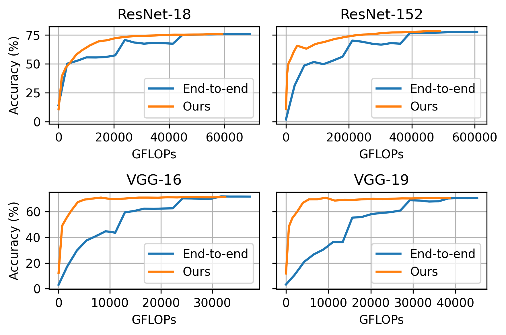
Figure 2: Accuracy (%) vs. GFLOPs on CIFAR-100 in the centralized setting.

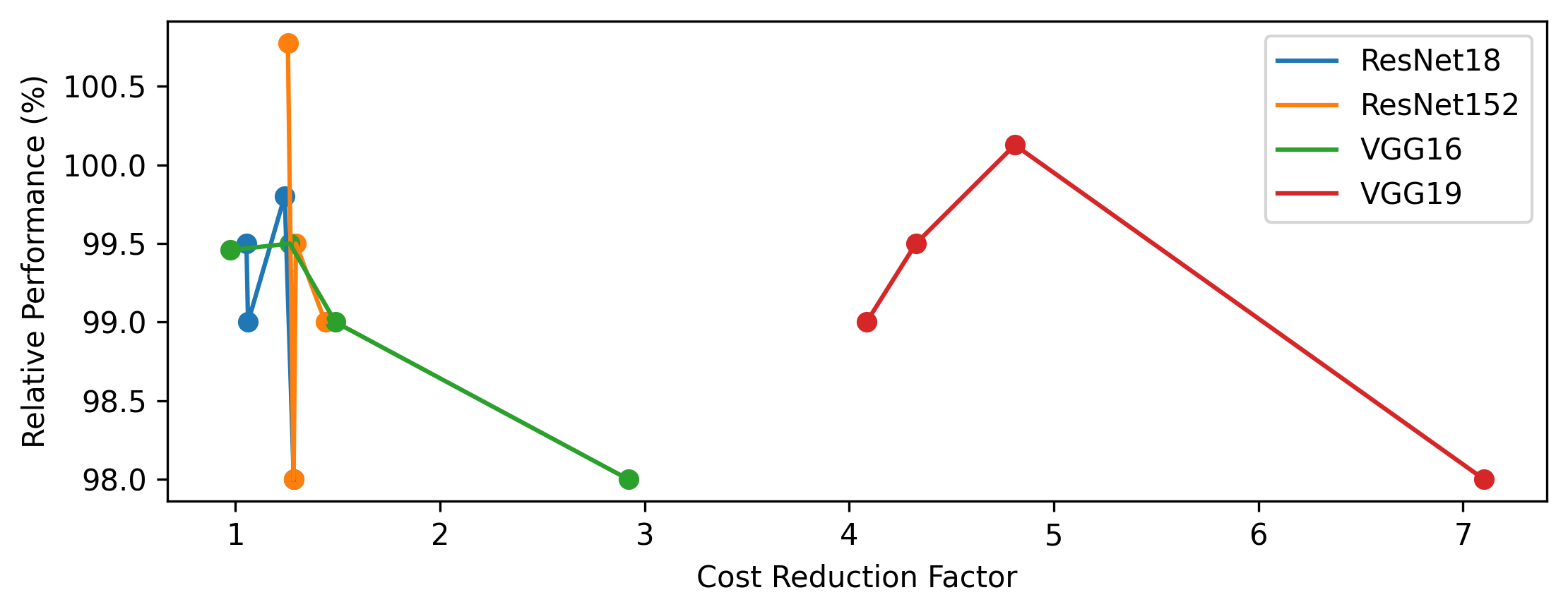
Figure 3: Computation cost reduction at $98\%$, $99\%$, $99.95\%$, best compared to the baseline (training full models) performance in the centralized setting on CIFAR-100.

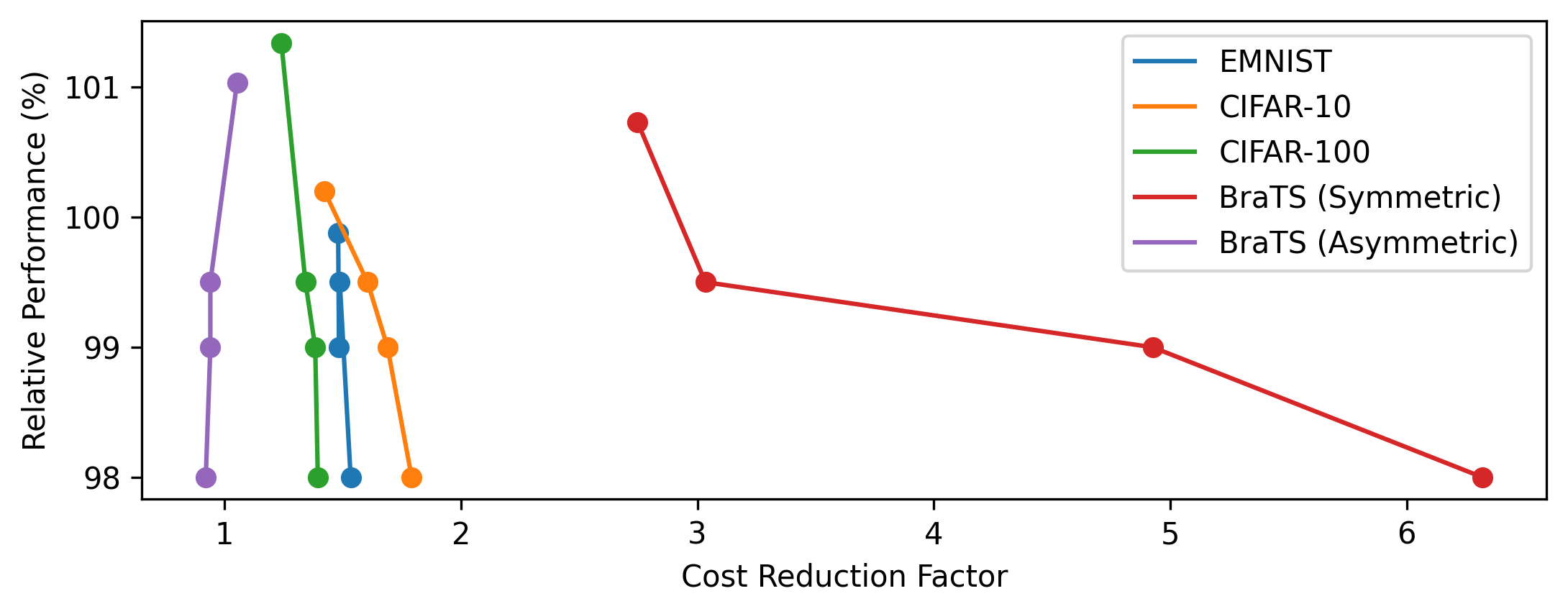
Figure 4: Communication cost reduction at $98\%$, $99\%$, $99.95\%$, best compared to the baseline performance in the federated setting.

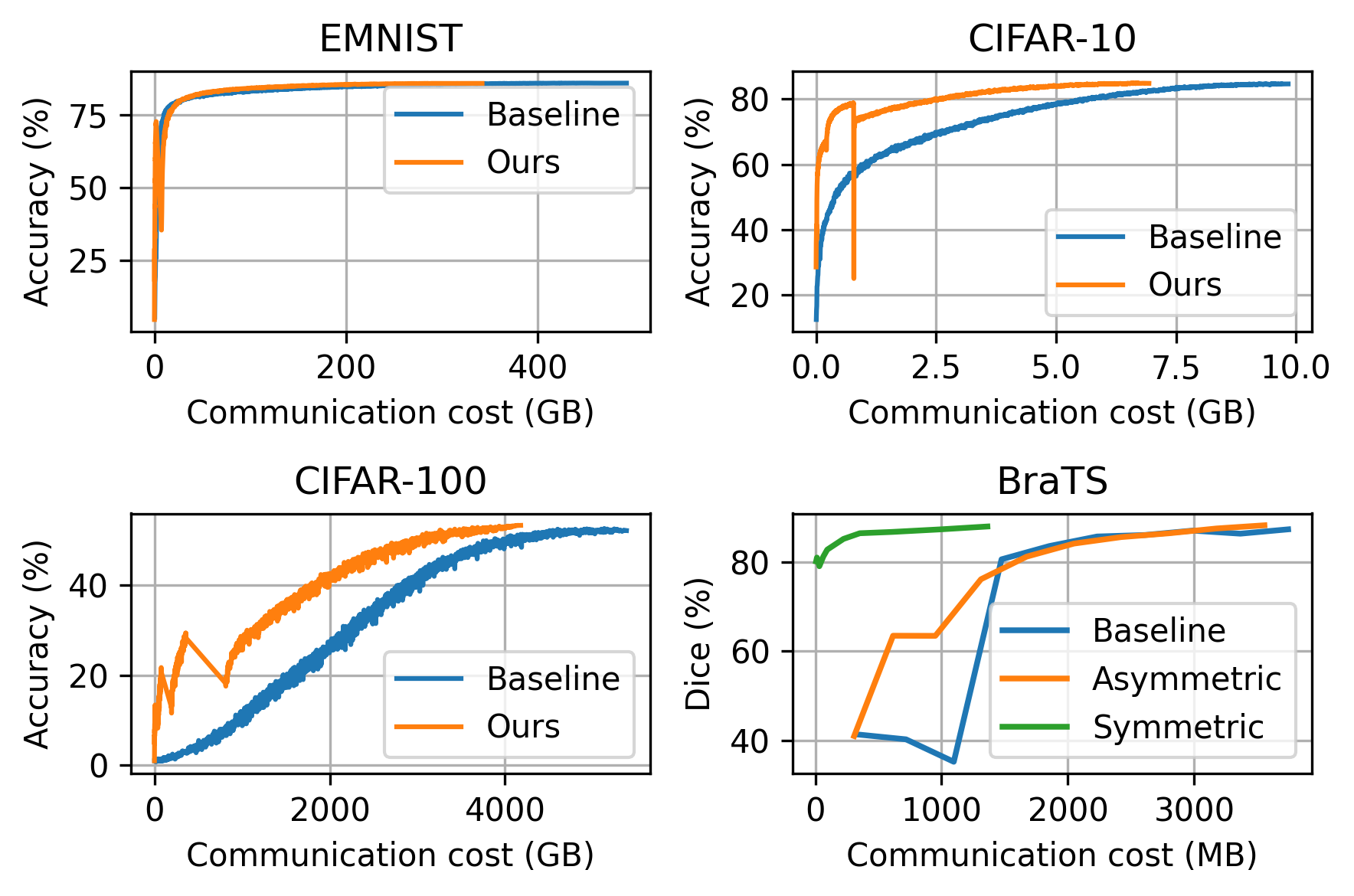
Figure 5: Communication cost vs. Accuracy (%) in federated settings on EMNIST (3400 clients, non-IID), CIFAR-10 (100 clients, IID), CIFAR-100 (500 clients, non-IID), and BraTS (10 clients, IID).

4.3 Communication Efficiency

We experiment in the federated setting to verify the communication efficiency of our method with FedAvg (McMahan et al., 2017). In particular, we consider classification tasks on three datasets, EMNIST, CIFAR-10, and CIFAR-100, and tumor segmentation tasks on the BraTS dataset. We follow the standard protocol as described in Section 4.1 to train the models and average the results over three random seeds. Results in Table 3 indicate that our method achieves comparable results on EMNIST and outperforms the baselines on all the other datasets. In addition, our method saves 20% to 30% two-way communication costs in classification and up to 63% costs in segmentation. The result simultaneously confirms the effectiveness and efficiency of our method. We discuss the effect of different numbers of stages in Section C.6.

Table 3: Results in federated settings. We report accuracy (%) for classification and Dice scores (%) for segmentation, followed by cost reduction (CR) as compared to the baselines (end-to-end).

	Baseline	Ours	CR
EMNIST	85.75 $\pm$ 0.11	85.67 $\pm$ 0.06	-29.49%
CIFAR-10	84.67 $\pm$ 0.14	84.85 $\pm$ 0.30	-29.70%
CIFAR-100	52.08 $\pm$ 0.44	53.23 $\pm$ 0.09	-22.90%
BraTS (Aym.)	86.77 $\pm$ 0.45	87.66 $\pm$ 0.49	-5.02%
BraTS (Sym.)	86.77 $\pm$ 0.45	87.96 $\pm$ 0.03	-63.60 %

We compare the performance at different communication costs in Figure 5. We observe that our method is communication-efficient over every cost budget, especially when the model parameters are not evenly distributed across sub-models. For instance, 3D-Unet has most of its parameters in the middle part of the model, making our Symmetric update strategy extremely efficient. On the other hand, the Asymmetric strategy shows marginal improvement since it starts from the heaviest portion of the model. The finding aligns with the motivation of progressive learning: learning from simpler models might facilitate training. We leave more analysis on segmentation in Section C.4.

Lastly, we analyze the cost reduction when achieving $98\%$, $99\%$, $99.5\%$, and the best of the performance of the converged baseline. This experiment studies the behavior of our method when only granted limited budgets. Figure 4 (and Figure 13 in the appendix that displays a larger range) presents that except for the Asymmetric strategy, our method improves communication efficiency across all datasets. In particular, it achieves practicable performance with 2x fewer costs in classification and up to 6.5x fewer costs in tumor segmentation. We also observe that the communication efficiency improves more when considering lower budgets. This property benefits when the time and communication budgets are limited (McMahan et al., 2017).

Table 4: Results of ProgFed with FedAvg, FedProx, and FedAdam on CIFAR-100 in the federated setting.

EMNIST
	FedAvg	FedProx	FedAdam
End-to-end	85.75	86.36	86.53
FedProg (S=4)	85.67	86.08	86.13
CIFAR-100
	FedAvg	FedProx	FedAdam
End-to-end	52.08	53.25	56.21
FedProg (S=4)	53.23	54.28	60.55

Table 5: Federated ResNet-18 on CIFAR-100 with compression. LQ-X denotes linear quantization followed by used bits representing gradients, and SP-X denotes sparsification followed by the percentage of kept gradients (see Table 11 for standard deviations).

	Float	LQ-8	LQ-4	LQ-2	SP-25	SP-10	LQ-8 +SP-25	LQ-8 +SP-10
	Accuracy (%)
Baseline	52.08	49.40	49.55	47.26	51.23	51.79	49.67	50.25
Ours	53.23	53.07	52.32	52.87	52.00	51.86	52.19	52.24
	Compression Cost (%)
Baseline	100	25.00	12.50	6.25	25.00	10.00	6.25	2.50
Ours	77.10	19.28	9.64	4.82	19.28	7.71	4.82	1.93

Table 6: Comparison between update strategies on CIFAR-100 with ResNet-18 in the centralized setting.

	Baseline	Ours	Layerwise	Partial	Mixed	Random
Accuracy (%)	76.08$\pm$0.12	75.84$\pm$0.28	72.40$\pm$0.16	74.70$\pm$0.04	75.04$\pm$1.26	74.38$\pm$0.97
Cost	1	0.86	1	1	$\approx 1$	0.88

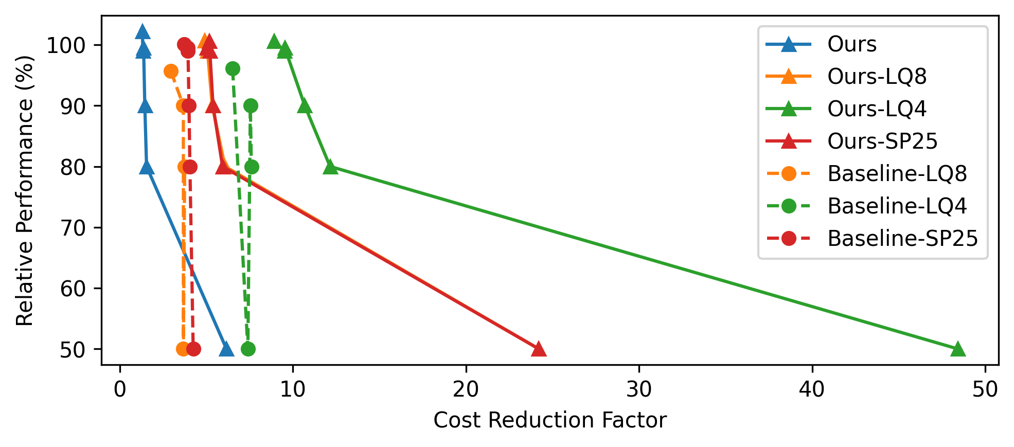
(a) Moderate compression

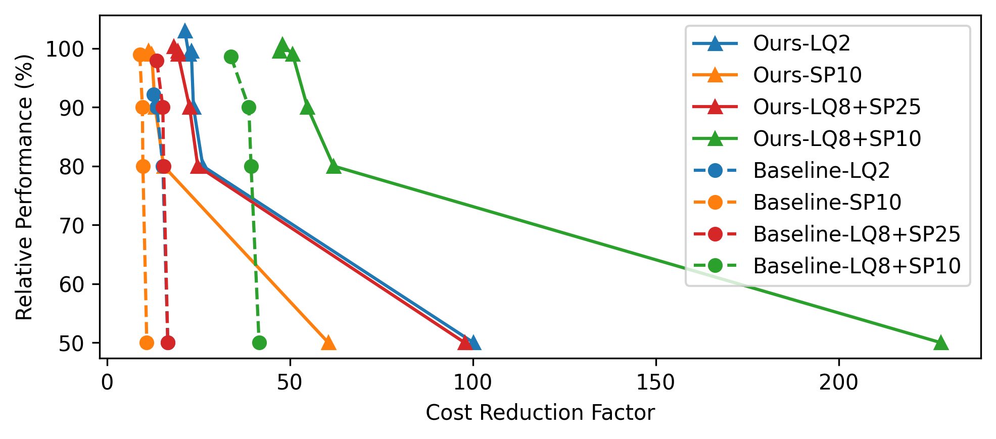
(b) Intensive compression

Figure 6: Relative performance vs. communication cost reduction with federated ResNet-18 on CIFAR-100 with (a) modest compression and (b) intensive compression.

4.4 Compatibility

Advanced optimization. We show that ProgFed can generalize to federated optimizations beyond FedAvg, including FedProx (Li et al., 2020) and FedAdam (Reddi et al., 2021), on CIFAR-100 and EMNIST. FedProx mitigates the non-IID problem by penalizing the L2 distance between the updated client models and the global model. On the other hand, FedAdam approaches the problem by adopting an Adam optimizer on the server side. These methods impose client-side and server-side regularization on top of FedAvg.

Results in Table 4 show that our method works seamlessly with FedProx and FedAdam. We first observe that the performance improves on both datasets when applying FedProx and FedAdam. Similar to the result in Table 3, our method significantly outperforms the baseline on CIFAR-100 while performing comparably on EMNIST. The result verifies that ProgFed can be readily applied to advanced federated optimizations.

Compression. We show that our method complements classical compression techniques including quantization and sparsification. We train several ResNet-18 on CIFAR-100 in the federated setting and apply linear quantization and sparsification following Konečnỳ et al. (2016). Specifically, we consider 8 bits, 4 bits, and 2 bits for quantization (denoted by LQ-X), 25% and 10% for sparsification (denoted by SP-X), and their combinations. Table 5 demonstrates the results. Our method clearly outperforms the baselines in all settings. It indicates that our method is more robust against compression errors, compatible with classical techniques, and thus permits a higher compression ratio.

In addition, we visualize 50%, 80%, 90%, 99%, 99.5%, and the best of the performance of the converged baseline against communication cost reduction in Figure 6. We observe that our method is more efficient across all percentages in every pair (Ours vs. Baseline, plotted in the same color). Besides, the baseline fails to achieve comparable performance in many settings, e.g., the ones with quantization, while our method retains comparable performance even with high compression ratios. Interestingly, even with additional compression, our method still facilitates learning at earlier stages. For example, Ours-LQ8+SP25 achieves comparable performance around 50x faster than the baseline, 60x faster to achieve 80%, and more than 200x faster to achieve 50% of performance. Overall, these properties grant our method to adequately approach limited network bandwidth and open up the possibility of more advanced compression schemes.

4.5 Analysis of ProgFed

Effect of norm discrepancy. As discussed in Section 3.2, the convergence rate of the full model is controlled by norm discrepancy, namely $q$. As $q_{t}$ approaches 1, the convergence rate will be closer to the convergence speed of the sub-models. We empirically evaluate the norm discrepancy on CIFAR-100 with ResNet-18 in the centralized setting. Figure 7 shows that the norm discrepancy decreases as the sub-models gradually recover the full model. It suggests that spending too much time on earlier stages may hurt the convergence speed while offering a higher compression ratio. This outlines the trade-off between communication and training efficiency.

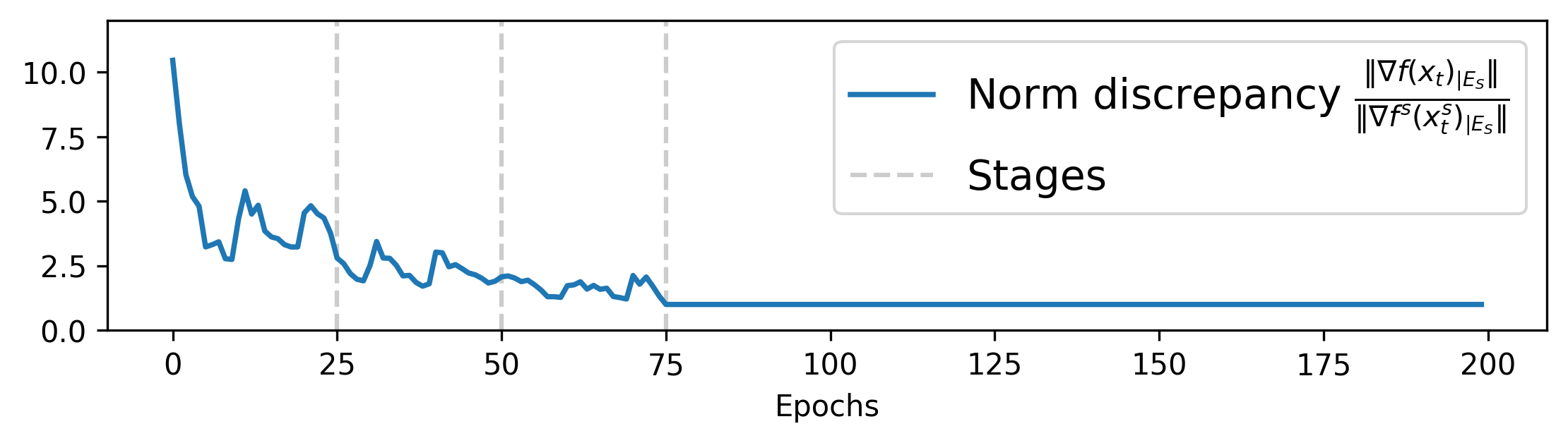
Figure 7: Norm discrepancy.

Comparison between update strategies. As described in Section 3, ProgFed progressively trains the network from the shallowest sub-model $\mathcal{M}^{1}$ to the full model $\mathcal{M}$. We verify our update strategy by comparing it with various baselines in the centralized setting. Baseline: end-to-end training; Layerwise only updates the latest layer $E_{i}$ while still passing the input through the whole model $\mathcal{M}$; Partial partially updates $E_{s}$ but acquires supervision from the last head $G_{S}$; Mixed combines Partial and Ours, trained on supervision from both $G_{i}$ and $G_{S}$; Random randomly chooses a sub-model $\mathcal{M}^{s}$ to update, rather than follows progressive learning.

Table 6 presents the performance and the computation cost ratio. We make several crucial observations. (1) Ours and Random do not pass the input through the whole network, making them consume fewer computation costs. (2) Layerwise greedily trains the network but achieves the worst performance, which highlights the importance of end-to-end fine-tuning. (3) Ours outperforms Random in both costs and accuracy, verifying the necessity of progressive learning. We also note that our method does not require additional memory space (compared to Random) and is easy to implement.

5 Discussion

There are two important hyperparameters $S$ and $\{T_{s}\}_{s=1}^{S}$ in ProgFed (Sec. 3.1). We note that hyperparameter selection in FL remains an open problem and could severely affect performance. For instance, Reddi et al. (2021) show that FL models are sensitive to learning rates. However, we show in Section C.6 that ProgFed works smoothly with various $s$ at the cost of slightly more epochs while still taking fewer costs to match the baseline performance. This aligns with Theorem 3.3 that ProgFed may take more epochs to converge but consume much fewer per-iteration costs. Lastly, we note that Theorem 3.3 is general for partial model updates. We leave incorporating structural updates and the non-IID data assumption for future work.

In addition to the efficiency and efficacy of ProgFed, we observe that the area under the curves of our method in Figure 2 and 5 are always larger than the end-to-end baselines. It suggests that our approach can provide more practical utility at all times. It aligns with the notion anytime learning (Caccia et al., 2021), where the models are expected to provide the best utility at any time during training. This feature is favorable in practice since users may access the system at any time of training, and ProgFed demonstrates great potential to implement such systems.

6 Conclusion

Beyond prior work on expressing models in compact formats, we show a novel approach to modifying the training pipeline to reduce the training costs. We propose ProgFed and show that progressive learning can be seamlessly applied to federated learning for communication and computation cost reduction. Extensive results on different architectures from small CNNs to U-Net and different tasks from simple classification to medical image segmentation show that our method is communication- and computation-efficient, especially when the training budgets are limited. Interestingly, we found that a progressive learning scheme has even led to improved performance in vanilla learning and more robust results when learning is perturbed e.g. in the case of gradient compression, which highlights progressive learning as a promising technique in itself with future application domains such as privacy-preserving learning, advanced compression schemes, and strong anytime-learning performance.

Appendix A Appendix

A.1 Proof of Theorem 3.3

In this section we prove Theorem 3.3. The proof builds on (Mohtashami et al., 2021) that considered training of subnetworks, but not the progressive learning case.

Lemma A.1.

Let $\mathbf{x}_{t}$ denote the weights of the full model, and $\mathbf{x}_{t}^{s}$ the weights of the model that is active in iteration $t$. Note that it holds $\mathbf{x}_{t\mid E_{s}}=\mathbf{x}^{s}_{t\mid E_{s}}$ as per the definition in the main text. It holds,

$$\mathds{E}f(\mathbf{x}_{t+1})\leq f(\mathbf{x}_{t})-\frac{\gamma}{2}\alpha^{2}_{t}\left\|\nabla f^{s}(\mathbf{x}_{t}^{s})_{\mid E_{s}}\right\|^{2}+\frac{\gamma^{2}L}{2}\sigma^{2}$$ (7)

Proof.

Let’s abbreviate $\mathbf{g}^{s}_{t}=g^{s}(\mathbf{x}_{t}^{s})$. By the update equation $\mathbf{x}_{t+1}^{s}=\mathbf{x}_{t}^{s}-\gamma_{t}\mathbf{g}^{s}_{t}$ it holds $\mathbf{x}_{t+1\mid E_{s}}=\mathbf{x}_{t\mid E_{s}}-\gamma_{t}\mathbf{g}^{s}_{t\mid E_{s}}$. With the $L$-smoothness assumption and the definition of $\alpha_{t}$,

$$\begin{split}\mathds{E}f(\mathbf{x}_{t+1})&\leq f(\mathbf{x}_{t})-\gamma_{t}\langle\nabla f(\mathbf{x}_{t})_{\mid E_{s}},\mathds{E}[\mathbf{g}^{s}_{t}]_{\mid E_{s}}\rangle+\frac{\gamma^{2}_{t}L}{2}\mathds{E}\left\|\mathbf{g}^{s}_{t\mid E_{s}}\right\|^{2}\\ &=f(\mathbf{x}_{t})-\gamma_{t}\langle\nabla f(\mathbf{x}_{t})_{\mid E_{s}},\mathds{E}[\mathbf{g}^{s}_{t}]_{\mid E_{s}}\rangle+\frac{\gamma^{2}_{t}L}{2}\mathds{E}(\left\|\mathbf{g}^{s}_{t\mid E_{s}}-\mathds{E}\mathbf{g}^{s}_{t\mid E_{s}}\right\|^{2}+\left\|\mathds{E}\mathbf{g}^{s}_{t\mid E_{s}}\right\|^{2})\\ &\leq f(\mathbf{x}_{t})-\gamma_{t}\langle\nabla f(\mathbf{x}_{t})_{\mid E_{s}},\nabla f^{s}(\mathbf{x}_{t}^{s})_{\mid E_{s}}\rangle+\frac{\gamma^{2}_{t}L}{2}\mathds{E}(\left\|\mathbf{g}^{s}-\mathds{E}\mathbf{g}^{s}_{t}\right\|^{2}+\left\|\nabla f^{s}(\mathbf{x}_{t}^{s})_{\mid E_{s}}\right\|^{2})\\ &\leq f(\mathbf{x}_{t})-\gamma_{t}\langle\nabla f(\mathbf{x}_{t})_{\mid E_{s}},\nabla f^{s}(\mathbf{x}_{t}^{s})_{\mid E_{s}}\rangle+\frac{\gamma^{2}_{t}L}{2}\left\|\nabla f^{s}(\mathbf{x}_{t}^{s})_{\mid E_{s}}\right\|^{2}+\frac{\gamma^{2}_{t}L}{2}\sigma^{2}\\ &\leq f(\mathbf{x}_{t})-\gamma_{t}\alpha_{t}(1-\frac{\gamma_{t}}{2\alpha_{t}}L)\left\|\nabla f^{s}(\mathbf{x}_{t}^{s})_{\mid E_{s}}\right\|^{2}+\frac{\gamma^{2}_{t}L}{2}\sigma^{2}\\ &\leq f(\mathbf{x}_{t})-\frac{\gamma_{t}}{2}\alpha_{t}\left\|\nabla f^{s}(\mathbf{x}_{t}^{s})_{\mid E_{s}}\right\|^{2}+\frac{\gamma^{2}_{t}L}{2}\sigma^{2}\\ &\leq f(\mathbf{x}_{t})-\frac{\gamma}{2}\alpha_{t}^{2}\left\|\nabla f^{s}(\mathbf{x}_{t}^{s})_{\mid E_{s}}\right\|^{2}+\frac{\gamma^{2}L}{2}\sigma^{2}\end{split}$$

Where in the last equation we used the facts that $\alpha_{t}\leq 1$ and $\gamma_{t}=\alpha_{t}\gamma$. ∎

We now prove Theorem 3.3.

Proof.

We first define $F_{t}\vcentcolon=\mathds{E}f(\mathbf{x}_{t})-(\min_{\mathbf{x}}f(\mathbf{x}))$. By rearranging Lemma A.1, we have

$$\frac{1}{2}\mathds{E}\alpha_{t}^{2}\left\|\nabla f^{s}(\mathbf{x}_{t}^{s})_{\mid E_{s}}\right\|^{2}\leq\frac{F_{t}-F_{t+1}}{\gamma}+\frac{\gamma L}{2}\sigma^{2}.$$ (8)

Next, with telescoping summation, we have

$$\frac{1}{T}\sum_{t=0}^{T-1}\mathds{E}\alpha_{t}^{2}\left\|\nabla f^{s}(\mathbf{x}_{t}^{s})_{\mid E_{s}}\right\|^{2}\leq\frac{2(F_{0}-F_{T-1})}{T\gamma}+\gamma L\sigma^{2}\leq\frac{2F_{0}}{T\gamma}+\gamma L\sigma^{2}$$ (9)

We now can prove the first of part Theorem 3.3 by setting the step size $\gamma$ to be $\mathcal{O}(\min\{\frac{1}{L},(\frac{F_{0}}{\sigma^{2}T})^{\frac{1}{2}}\}$ as in (Mohtashami et al., 2021).

To prove the convergence of the model of interest (the second part),

$$\begin{split}\frac{1}{T}\sum_{t=0}^{T-1}\left\|\nabla f(\mathbf{x}_{t})\right\|^{2}&=\frac{1}{T}\sum_{t=0}^{T-1}\frac{\left\|\nabla f(\mathbf{x}_{t})\right\|^{2}}{\alpha^{2}_{t}\left\|\nabla f^{s}(\mathbf{x}_{t}^{s})_{\mid E_{s}}\right\|^{2}}\alpha_{t}^{2}\left\|\nabla f^{s}(\mathbf{x}^{s}_{t})_{\mid E_{s}}\right\|^{2}\\ &=\frac{1}{T}\sum_{t=0}^{T-1}q_{t}^{2}\alpha^{2}_{t}\left\|\nabla f^{s}(\mathbf{x}_{t}^{s})_{\mid E_{s}}\right\|^{2}\leq q^{2}\frac{1}{T}\sum_{t=0}^{T-1}\alpha^{2}_{t}\left\|\nabla f^{s}(\mathbf{x}_{t}^{s})_{\mid E_{s}}\right\|^{2}\end{split}$$ (10)

where

$$q_{t}=\frac{\left\|\nabla f(\mathbf{x}_{t})\right\|}{\alpha_{t}\left\|\nabla f^{s}(\mathbf{x}_{t}^{s})_{\mid E_{s}}\right\|}\qquad\text{and}\qquad q=\max_{t\in[T]}q_{t}.$$ (11)

By definition $q\geq q_{t}$ for all $t\in[T]$, we reach the last inequality and combine it with the first part of the theorem.

$$\frac{1}{T}\sum_{t=0}^{T-1}\alpha^{2}_{t}\left\|\nabla f^{s}(\mathbf{x}_{t})\right\|^{2}\leq\frac{\epsilon}{q^{2}}$$ (12)

∎

Using $\frac{\epsilon}{q^{2}}$ as the new threshold, we immediately prove the second part.

Appendix B Implementation details

We describe details of the datasets used in Section 4 and present the hyper-parameters in Table 7.

Table 7: Parameters for federated experiments

Dataset	#clients	#clients_per_epoch	batch_size	#epochs
EMNIST	3400	68	20	1500
CIFAR-10	100	10	50	2000
CIFAR-100	500	40	20	3000
BraTS	10	10	3	100
	#epoch_per_client	#stages ($S$)	$T_{s}$	#epochs_for_warmup
EMNIST	1	3	250	5
CIFAR-10	5	4	250	0
CIFAR-100	1	4	375	25
BraTS	3	4	25	0

CIFAR-10. We conduct experiments on CIFAR-10 datasets for federated learning, following the setup of previous work (McMahan et al., 2017). The dataset is divided into 100 clients randomly, namely iid distributions for every client. We adopt the same CNN architecture with 122,570 parameters.

CIFAR-100. We follow the federated learning benchmark of CIFAR-100 proposed in (Reddi et al., 2021) to conduct the experiments on CIFAR-100. We use ResNet-18/-152 (batch norm are replaced with group norm (Hsieh et al., 2020)) and VGG-16/-19 in the centralized setting, while only considering ResNet-18 in the federated experiments. This setup allows us to evaluate the federated learning systems on non-IID distributions, where we use the splits as suggested in (Reddi et al., 2021).

EMNIST. We follow the benchmark setting in (Reddi et al., 2021) to experiment. There are 3,400 clients and 671,585 training examples distributed in a non-iid fashion. The models are eventually evaluated on 77,483 examples, resulting in a challenging task.

BraTS. In addition to image classification, we conduct experiments on brain tumor segmentation based on (Sheller et al., 2020). We train a 3D-Unet on the BraTS2018 dataset, which includes 285 MRI scans annotated by five classes of labels. The network has 9,451,567 parameters. The training set is randomly partitioned into ten clients. All clients participate in every training round and locally train their models for three local epochs. This setting matches the practical medical applications. Institutions often own relatively stable network conditions, and the data are rare and of high resolution.

Architectures. ConvNets for EMNIST and MNIST consist of two convolution layers, termed Conv1 and Conv2, followed by two fully connected layers, termed FC1 and FC2. To apply progressive learning with $S=3$, we set Conv1, Conv2, FC1 to be the three stages, namely $E_{i}$, and FC2 to the final head, namely $G_{S}$. As for VGGs, we divide the whole networks into five components according to the max-pooling layers. We combine the first two to be $E_{1}$ and set the others to be the remaining $E_{i}$ under the setting $S=4$. To apply ProgFed to ResNets (He et al., 2016), we first replace the batch normalization layers with group normalization. By convention, ResNets have five convolution components, i.e. Conv1, Conv2_x, Conv3_x, Conv4_x, and Conv5_x. We combine Conv1 and Conv2_x to be $E_{1}$ and all the other components to be the remaining $E_{i}$. It thus matches $S=4$ in our setting.

Appendix C More Results

C.1 Comparison between update strategies

As described in Section 4.5, we compare ProgFed to other baselines. We additionally report the performance vs. computation costs and performance vs. epochs in Figure 8, where Ours reaches comparable performance while consuming the least cost.

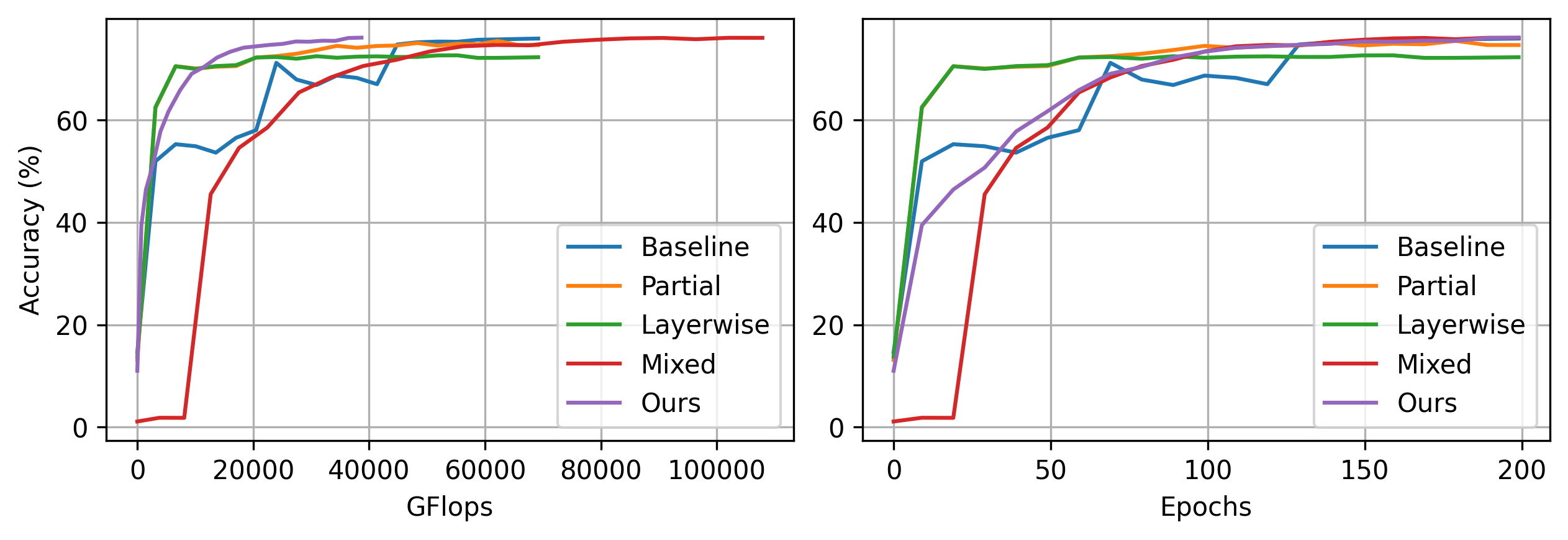
Figure 8: Performance vs. computation costs and Performance vs. epochs when comparing our method to different updating strategies.

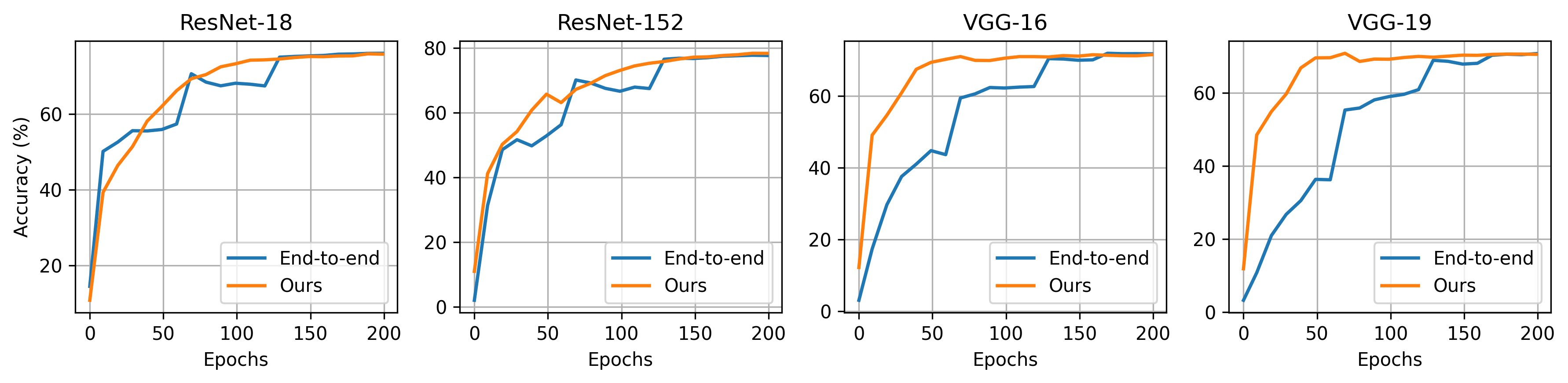
Figure 9: Accuracy (%) vs. Epochs on CIFAR-100 in the centralized setting.

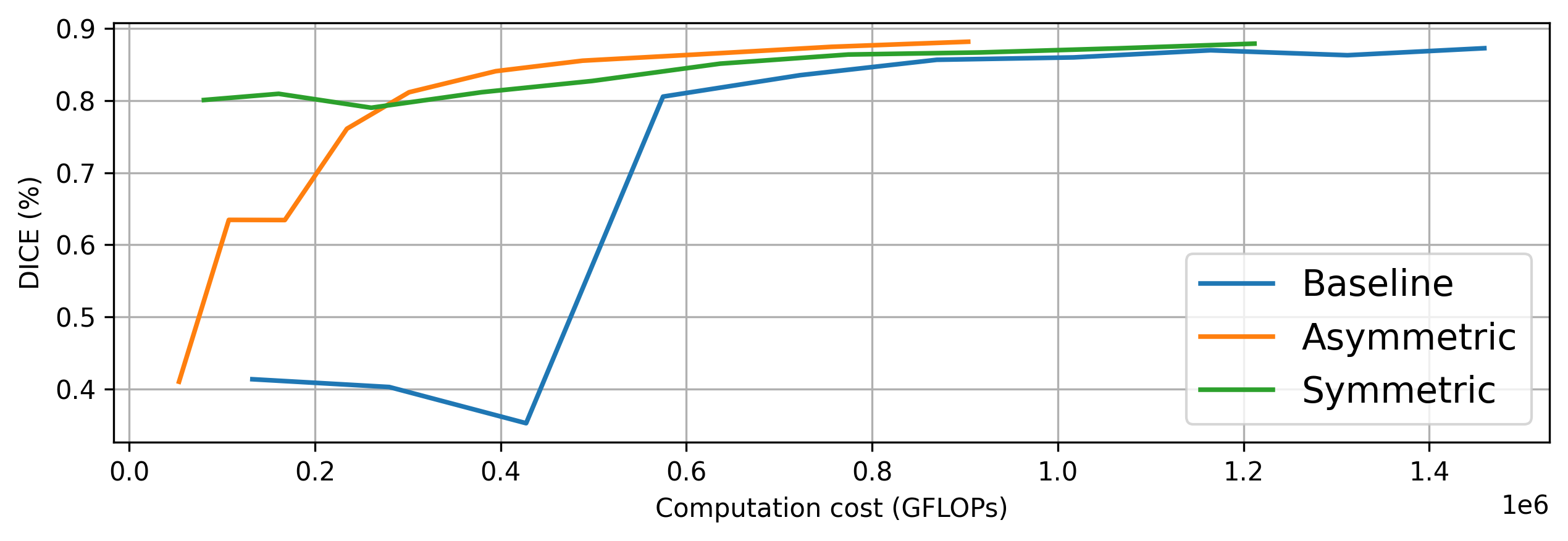
Figure 10: DICE (%) vs. computation costs on BraTS.

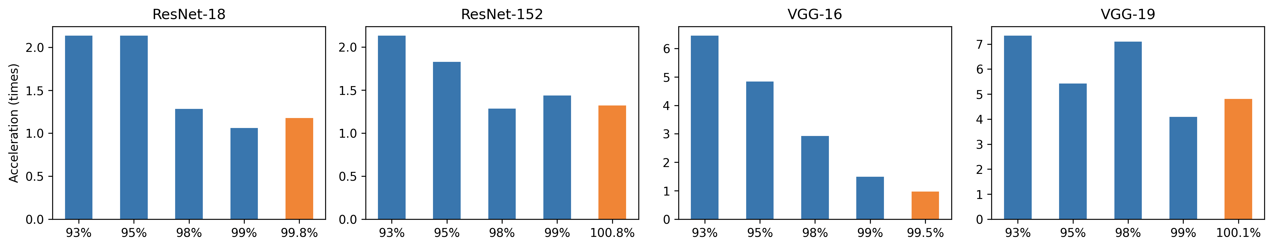
Figure 11: Computation acceleration at different percentage of performance. The orange bar indicates the best performance of our method.

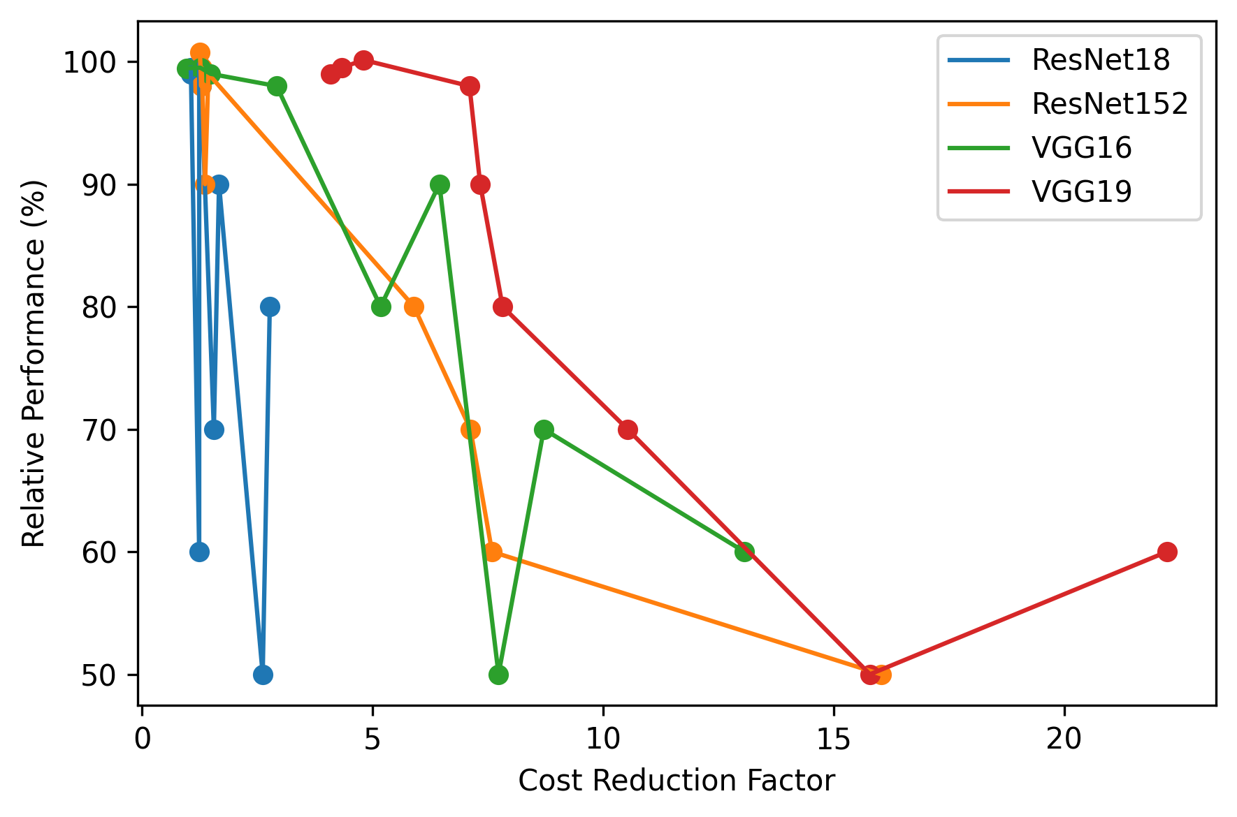
Figure 12: Computation cost reduction at $\{50\%$, $60\%$, $70\%$, $80\%$, $90\%$ $98\%$, $99\%$, $99.95\%$, $\textit{best}\}$ of the baseline performance in the centralized setting.

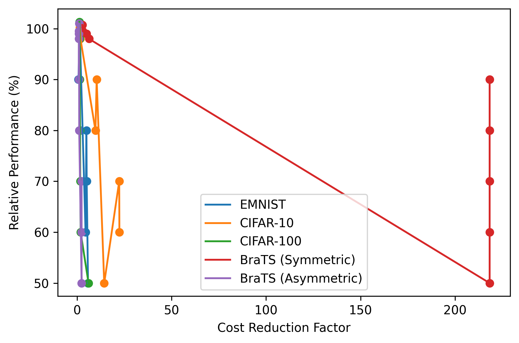
Figure 13: Communication cost reduction at $\{50\%$, $60\%$, $70\%$, $80\%$, $90\%$ $98\%$, $99\%$, $99.95\%$, $\textit{best}\}$ of the baseline performance in the federated setting.

C.2 Computation Efficiency

We present more experiments in the centralized setting to prove the computation efficiency of our method. Figure 9 presents accuracy vs. epochs with four architectures on CIFAR-100. The result indicates that our method converges comparably faster to end-to-end training in practice. Figure 11 presents Figure 3 in bar charts. Similar to Figure 3, our method improves across architectures while VGGs benefit even more from our method. Figure 10 presents the computation costs of 3D-Unets on the BraTS dataset. We make the first observation that tumor segmentation requires heavy computation. Interestingly, even though the earlier stages of Symmetric consume much fewer communication costs (Figure 5), they require more computation costs than Asymmetric. It might root from the higher resolution of feature maps that Symmetric keeps and thus lead to a trade-off between communication and computation costs.

Figure 11 extend Figure 3 to a larger range $\{50\%$, $60\%$, $70\%$, $80\%$, $90\%$ $98\%$, $99\%$, $99.95\%$, $\textit{best}\}$. The result shows that our method benefits across models and is especially efficient when training budgets are limited.

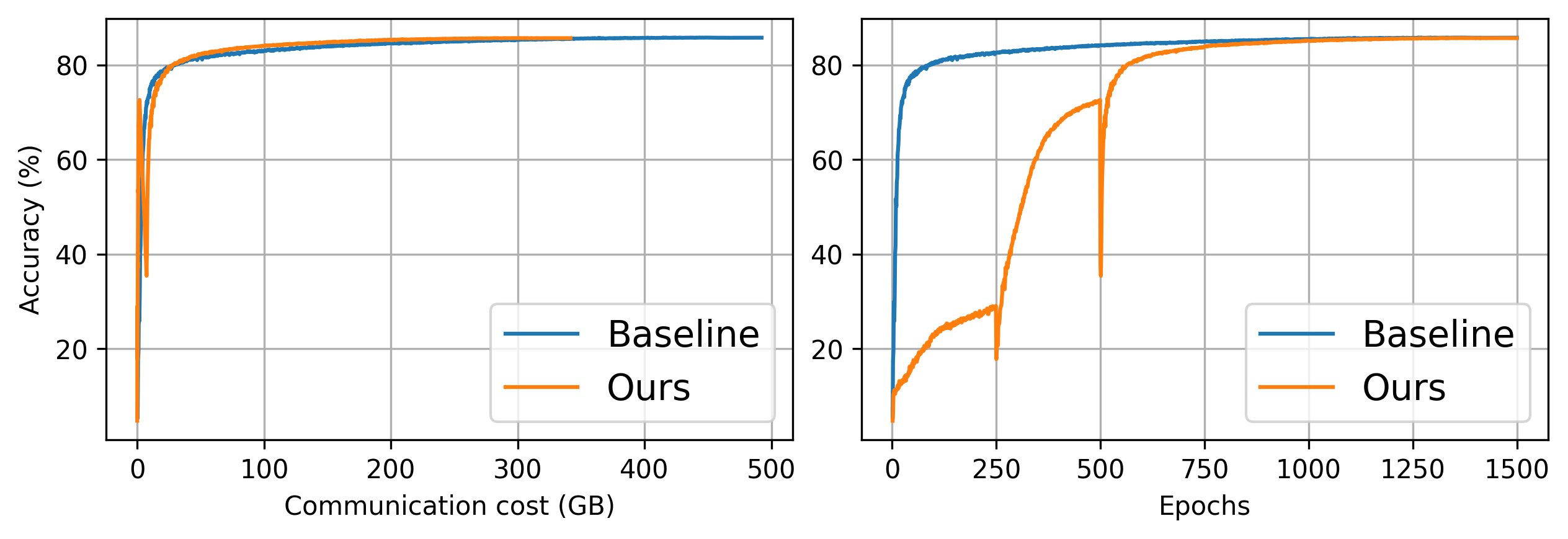
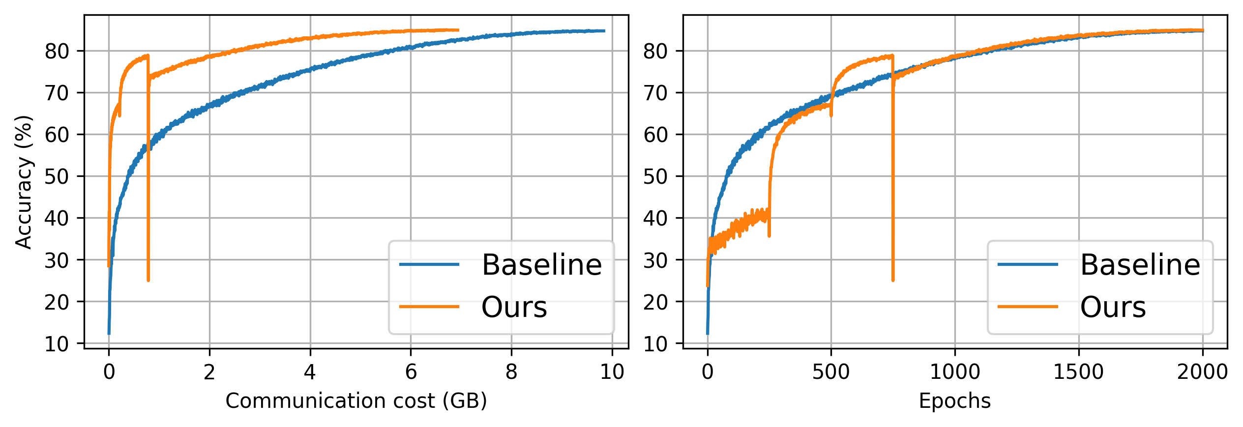
(a) ConvNet on EMNIST	(b) ConvNet on CIFAR-10
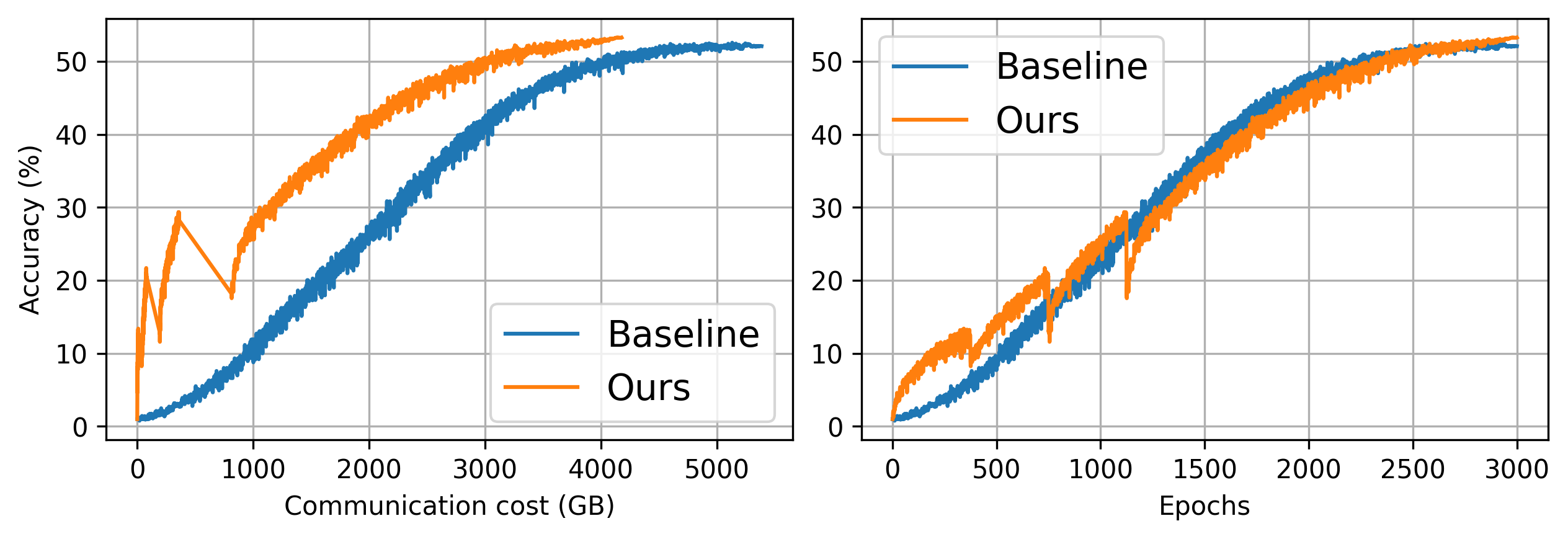
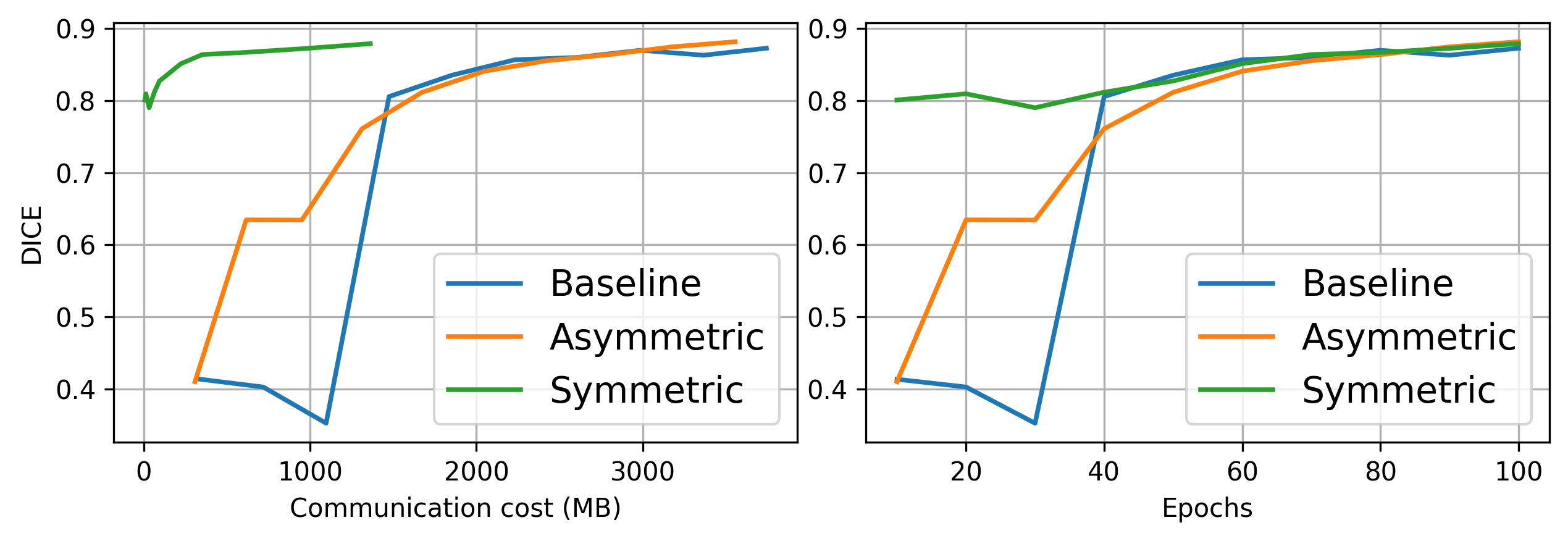
(c) ResNet-18 on CIFAR-100	(d) 3D-Unet on BraTS

Figure 14: Accuracy vs. computation costs and accuracy vs. epochs in the federated setting. (a)(b)(c) shows the result for three classification tasks; (d) shows the result for the segmentation task, where two update strategies Symmetric and Asymmetric are adopted for 3D-Unet.

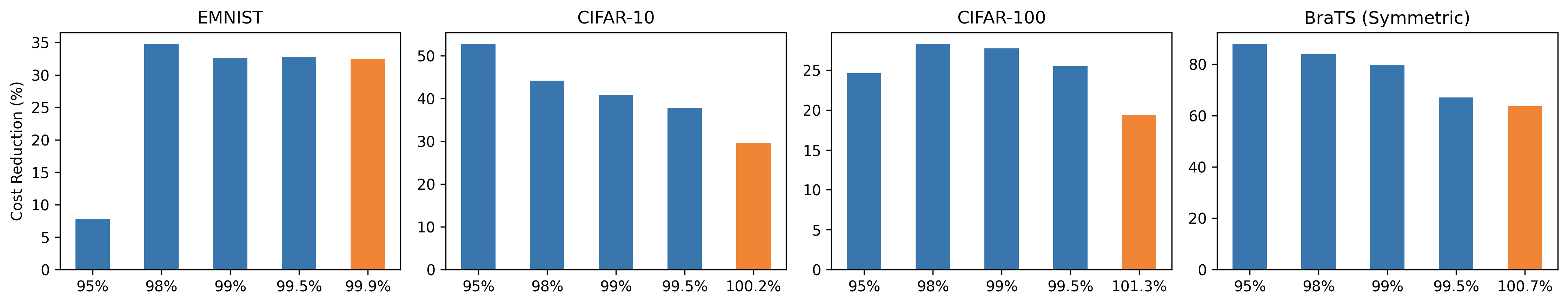
Figure 15: Communication cost reduction at different percentage of performance. The orange bar indicates the best performance of our method.

C.3 Communication Efficiency

We present more experiments in the federated setting to prove the communication efficiency of our method. To complement Figure 5, we additionally visualize performance vs. communication costs and performance vs. epochs in Figure 14. Although our method causes performance fluctuation in some datasets, the performance recovers very quickly. Figure 15 presents Figure 4 in bar charts. The results show that our method saves considerable costs in almost all settings except for EMNIST at 95%. It is because both baseline and our method improve fast at the beginning while our method stands out in the latter phase of training (e.g. after 98%). The result also supports that our method improves across datasets.

We present Figure 4 in a region that models are applicable. Here, we plot the figure with a larger range $\{50\%$, $60\%$, $70\%$, $80\%$, $90\%$ $98\%$, $99\%$, $99.95\%$, $\textit{best}\}$ in Figure 13. The result is consistent, showing that our method benefits across datasets, and is efficient when granted limited training budgets.

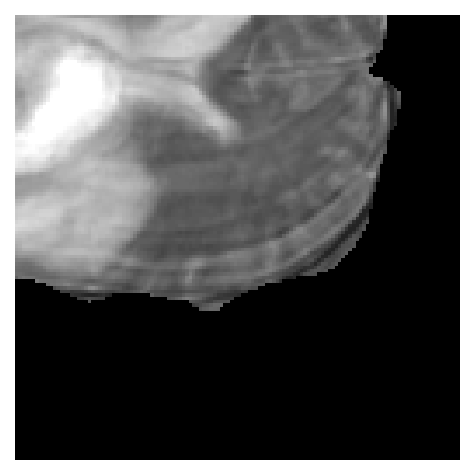
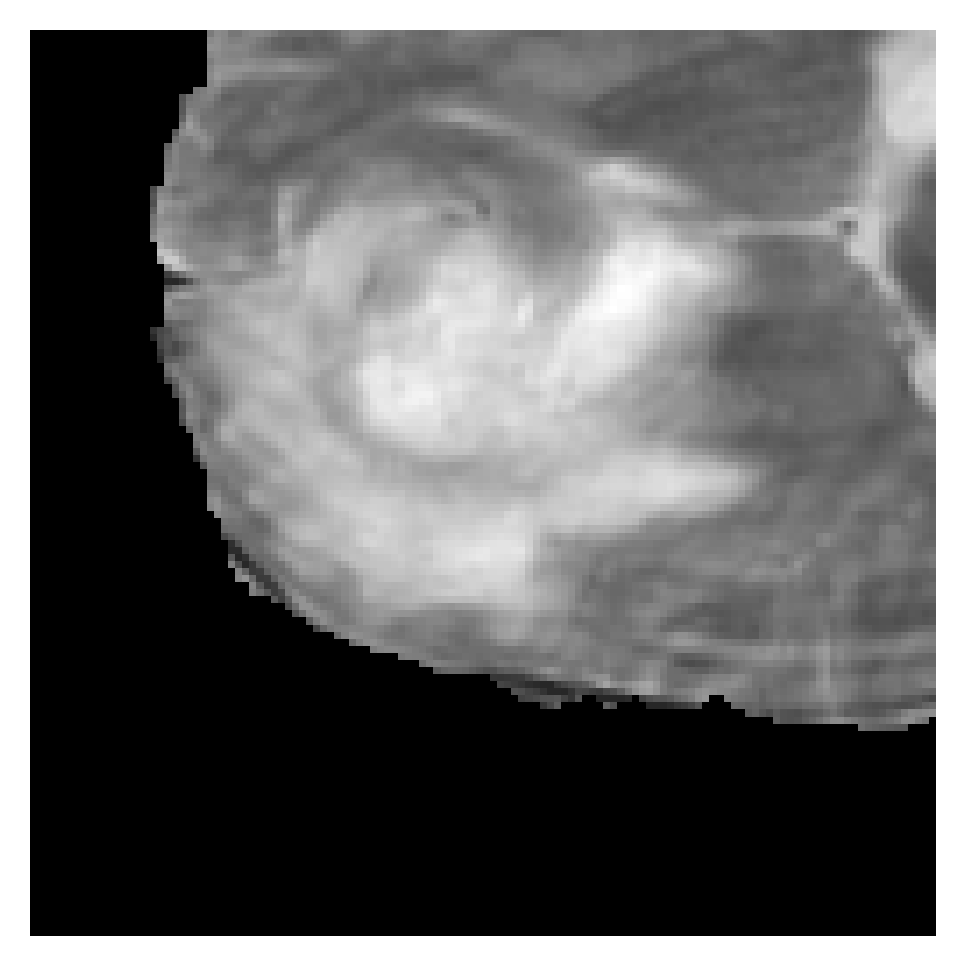
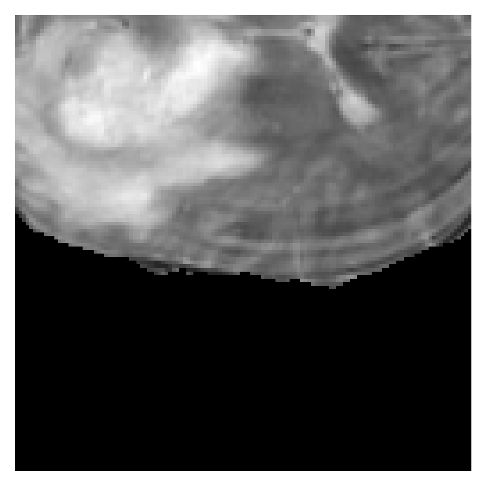
Input	Ground Truth	Baseline (100%)	Asymmetric (94.98%)	Symmetric (36.40%)

Figure 16: Visualization of federated segmentation. From left to right: Input, Ground Truth, Baseline, Asymmetric, and Symmetric updating strategies. Despite the comparable performance, Symmetric consumes significantly fewer communication costs.

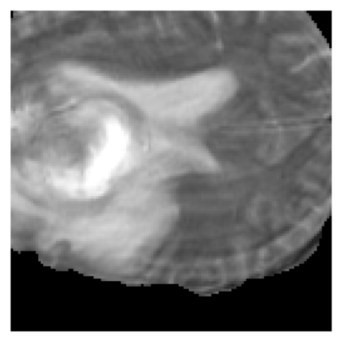
Input	$\approx 0.18\%$	$\approx 9.40\%$	$\approx 36.40\%$	Ground Truth

Figure 17: Segmentation results under {$\approx 0.18\%$, $\approx 9.40\%$ , $\approx 36.40\%$} of communication costs of the converged baseline. From top to bottom: baseline, Asymmetric (Ours), and Symmetric (Ours). Only Symmetric can achieve $0.18\%$ (6.7536 MB) compression ratio, since the size of the other models is already around 34 MB (i.e. $0.908\%$).

C.4 Visualization of Federated Segmentation

We visualize the outputs of 3D-Unet (see Section 4.3) in Figure 16. The result matches the number reported in Table 3 that the models perform similarly after they have converged. However, the communication cost consumption is disparate. Symmetric only consumes $36.40\%$ while the others either do not save any cost or marginally improve it. We visualize the results in Figure 17 when granted limited communication budgets. Note that even with the same cost, Symmetric and Asymmetric may stay in different stages because Symmetric starts from the outer part, consisting of significantly fewer parameters. We find that Baseline and Asymmetric fail to compress the models with $0.18\%$ since their models are of size 34 MB (i.e. $0.908\%$), while only Symmetric achieve it. Interestingly, Symmetric has produced promising results at $0.18\%$ of costs. It suggests that our method significantly facilitates learning even given limited communication budgets. Meanwhile, we hope these findings could inspire more further work on medical learning problems.

Table 8: Raw results on CIFAR-100 with four architectures in the centralized setting (to complement Table 2).

	End-to-End					ProgFed (Ours)
	Seed1	Seed2	Seed3	Mean	Std	Seed1	Seed2	Seed3	Mean	Std
ResNet-18	75.95	76.12	76.17	76.08	0.12	75.57	76.13	75.83	75.84	0.28
ResNet-152	77.69	77.44	78.19	77.77	0.38	78.95	78.46	78.31	78.57	0.33
VGG16 (bn)	71.94	71.77	71.65	71.79	0.15	71.36	72.05	71.21	71.54	0.45
VGG19 (bn)	69.47	71.25	71.70	70.81	1.18	71.30	70.45	70.95	70.90	0.43

Table 9: Raw results in federated settings on EMNIST, CIFAR-10, and CIFAR-100 (to complement Table 3).

	EMNIST
	Seed1	Seed2	Seed3	Mean	Std
Baseline	85.63	85.77	85.85	85.75	0.11
Ours	85.65	85.62	85.73	85.67	0.06
	CIFAR-10
	Seed1	Seed2	Seed3	Mean	Std
Baseline	84.62	84.82	84.56	84.67	0.14
Ours	84.64	84.73	85.19	84.85	0.30
	CIFAR-100
	Seed1	Seed2	Seed3	Mean	Std
Baseline	51.79	51.86	52.58	52.08	0.44
Ours	53.33	53.16	53.21	53.23	0.09

Table 10: Raw results on BraTS in the federated setting (to complement Table 3).

	Seed 1	Seed 2	Seed 3	Mean	Std
Baseline	87.29	86.51	86.51	86.77	0.45
Idea1 (Ours)	88.19	87.22	87.57	87.66	0.49
Idea2 (Ours)	87.92	87.98	87.98	87.96	0.03

Table 11: Federated ResNet-18 on CIFAR-100 with compression. LQ-X denotes linear quantization followed by used bits representing gradients, and SP-X denotes sparsification followed by the percentage of kept gradients. (to complement Table 5).

	Float	LQ-8	LQ-4	LQ-2
	Accuracy (%)
Baseline	52.08 $\pm$ 0.44	49.40 $\pm$ 0.75	49.55 $\pm$ 0.59	47.26 $\pm$ 0.29
Ours	53.23 $\pm$ 0.09	53.07 $\pm$ 1.00	52.32 $\pm$ 0.15	52.87 $\pm$ 0.54
	Compression ratio (%)
Baseline	100	25.00	12.50	6.25
Ours	77.10	19.28	9.64	4.82
	SP-25	SP-10	LQ-8 +SP-25	LQ-8 +SP-10
	Accuracy (%)
Baseline	51.23 $\pm$ 0.56	51.79 $\pm$ 0.10	49.67 $\pm$ 1.58	50.25 $\pm$ 1.03
Ours	52.00 $\pm$ 0.19	51.86 $\pm$ 0.23	52.19 $\pm$ 0.03	52.24 $\pm$ 0.12
	Compression ratio (%)
Baseline	25.00	10.00	6.25	2.50
Ours	19.28	7.71	4.82	1.93

C.5 Raw numbers and more statistics

Table 8 9, and 10 present the raw numbers of the experiments in Table 2 and 3 over three random seeds. Table 11 presents the standard deviations of Table 5 over three random seeds.

Table 12: Ablation study on numbers of stages with different numbers of total epochs on CIFAR-100.

	Accuracy (%)	Cost (GB)	Accuracy (%)	Cost (GB)
	#epoch=3000		#epoch=4000
End-to-End	52.08	5368	-	-
ProgFed (S=3)	51.33	4418	53.80	5695
ProgFed (S=4)	53.23	4179	-	-
ProgFed (S=5)	51.53	4264	54.25	5479
ProgFed (S=8)	50.70	3901	54.46	5166

Table 13: Communication costs of ProgFed when achieving the performance of end-to-end training (52.08%).

	#Total_epochs	Cost
End-to-End	3000	5368
ProgFed (S=3)	4000	4365
ProgFed (S=4)	3000	3804
ProgFed (S=5)	4000	3781
ProgFed (S=8)	4000	3421

Table 14: Performance of ProgFed when consuming the same amount of communication costs as S=4 and #Total_epochs = 3000 (4179GB).

	#Total_epochs	Accuracy (%)
End-to-end	3000	51.19
ProgFed (S=3)	4000	52.33
ProgFed (S=4)	3000	53.23
ProgFed (S=5)	4000	53.56
ProgFed (S=8)	4000	53.50

C.6 Ablation study on the number of stages

We conduct an ablation study on CIFAR-100 with ResNet-18 to verify the influence of different numbers of stages $S$, namely $S=3$, $4$, $5$, and $8$. We set the remaining hyper-parameters as discussed in Section 3.1 to ensure a fair comparison. Table 12 shows that $S=4$ performs the best among all settings when the number of total epochs is equal to 3000. However, Theorem 3.3 suggests that ProgFed could be at most two times slower than the end-to-end training. Therefore, we show that the performance immediately improves if we slightly increase the number of total epochs. Table 12 summarizes the result. Despite the improved performance, the final costs also increase subsequently.

To fairly compare these two settings, we summarize the results in Table 13 when all settings achieve the end-to-end baseline performance (52.08%). It is observed that all settings, including those with more epochs, achieve the same performance as the baseline at much fewer costs. Moreover, the cost decreases as the number of stages $S$ increases. On the other hand, we report the performance when all settings consume the same amount of costs as $S=4$ with 3000 epochs. Table 14 shows that all settings perform better than the baseline and similarly well except $S=3$. It might indicate that ProgFed is insensitive to $S$ and the number of total epochs when given the same budget.

Appendix D More Related work

We discuss more related work in this section.

Model pruning. Model pruning removes redundant weights to address the resource constraints (Mozer & Smolensky, 1989; LeCun et al., 1990; Frankle & Carbin, 2019; Lin et al., 2019). There are two categories: unstructured and structured pruning. Unstructured methods prune individual model weights according to certain criteria such as Hessian of the loss function (LeCun et al., 1990; Hassibi & Stork, 1993) and small magnitudes (Han et al., 2015). However, these methods cannot fully accelerate without dedicated hardware since they often result in sparse weights. In contrast, structured pruning methods prune channels or even layers to alleviate the issue. They often learn importance weights for different components and only keep relatively important ones (Liu et al., 2017; Yu et al., 2018; Mohtashami et al., 2021; Li et al., 2021). Despite the efficiency, model pruning usually happens at inference and does not reduce training costs while our method achieves computation- and communication-efficiency even during training.

Model distillation. Another line of research for model compression is model distillation (Buciluǎ et al., 2006; Hinton et al., 2015), which requires a student model to mimic the behavior of a teacher model (Polino et al., 2018; Sun et al., 2019). Recent work has investigated transmitting logits rather than gradients (Li & Wang, 2019; Lin et al., 2020; He et al., 2020; Choquette-Choo et al., 2020), which significantly reduces communication costs. However, these methods either require additional query datasets (Li & Wang, 2019; Lin et al., 2020) or cannot enjoy the merit of datasets from different sources (Choquette-Choo et al., 2020). In contrast, our work reduces the costs while retaining the dataset efficiency.

References

- Alistarh et al. (2017) Alistarh, D., Grubic, D., Li, J., Tomioka, R., and Vojnovic, M. Qsgd: Communication-efficient sgd via gradient quantization and encoding. Advances in Neural Information Processing Systems (NeurIPS), 30:1709–1720, 2017.
- Bakas et al. (2017) Bakas, S., Akbari, H., Sotiras, A., Bilello, M., Rozycki, M., Kirby, J. S., Freymann, J. B., Farahani, K., and Davatzikos, C. Advancing the cancer genome atlas glioma mri collections with expert segmentation labels and radiomic features. Scientific data, 4(1):1–13, 2017.
- Bakas et al. (2018) Bakas, S., Reyes, M., Jakab, A., Bauer, S., Rempfler, M., Crimi, A., Shinohara, R. T., Berger, C., Ha, S. M., Rozycki, M., et al. Identifying the best machine learning algorithms for brain tumor segmentation, progression assessment, and overall survival prediction in the brats challenge. arXiv preprint arXiv:1811.02629, 2018.
- Belilovsky et al. (2020) Belilovsky, E., Eickenberg, M., and Oyallon, E. Decoupled greedy learning of cnns. In Proceedings of the International Conference on Machine Learning (ICML), pp. 736–745. PMLR, 2020.
- Bernstein et al. (2018) Bernstein, J., Wang, Y.-X., Azizzadenesheli, K., and Anandkumar, A. signsgd: Compressed optimisation for non-convex problems. In Proceedings of the International Conference on Machine Learning (ICML), pp. 560–569. PMLR, 2018.
- Buciluǎ et al. (2006) Buciluǎ, C., Caruana, R., and Niculescu-Mizil, A. Model compression. In Proceedings of the 12th ACM SIGKDD international conference on Knowledge discovery and data mining, pp. 535–541, 2006.
- Caccia et al. (2021) Caccia, L., Xu, J., Ott, M., Ranzato, M., and Denoyer, L. On anytime learning at macroscale. arXiv preprint arXiv:2106.09563, 2021.
- Choquette-Choo et al. (2020) Choquette-Choo, C. A., Dullerud, N., Dziedzic, A., Zhang, Y., Jha, S., Papernot, N., and Wang, X. Capc learning: Confidential and private collaborative learning. In Proceedings of the International Conference on Learning Representations (ICLR), 2020.
- Cohen et al. (2017) Cohen, G., Afshar, S., Tapson, J., and Van Schaik, A. Emnist: Extending mnist to handwritten letters. In 2017 International Joint Conference on Neural Networks (IJCNN), pp. 2921–2926. IEEE, 2017.
- DeVries & Taylor (2017) DeVries, T. and Taylor, G. W. Improved regularization of convolutional neural networks with cutout. arXiv preprint arXiv:1708.04552, 2017.
- Frankle & Carbin (2019) Frankle, J. and Carbin, M. The lottery ticket hypothesis: Finding sparse, trainable neural networks. In Proceedings of the International Conference on Learning Representations (ICLR), 2019. URL https://openreview.net/forum?id=rJl-b3RcF7.
- Fu et al. (2020) Fu, F., Hu, Y., He, Y., Jiang, J., Shao, Y., Zhang, C., and Cui, B. Don’t waste your bits! squeeze activations and gradients for deep neural networks via tinyscript. In Proceedings of the International Conference on Machine Learning (ICML), pp. 3304–3314. PMLR, 2020.
- Goyal et al. (2017) Goyal, P., Dollár, P., Girshick, R., Noordhuis, P., Wesolowski, L., Kyrola, A., Tulloch, A., Jia, Y., and He, K. Accurate, large minibatch sgd: Training imagenet in 1 hour. arXiv preprint arXiv:1706.02677, 2017.
- Han et al. (2015) Han, S., Pool, J., Tran, J., and Dally, W. Learning both weights and connections for efficient neural network. Advances in Neural Information Processing Systems (NeurIPS), 28, 2015.
- Hassibi & Stork (1993) Hassibi, B. and Stork, D. G. Second order derivatives for network pruning: Optimal brain surgeon. Morgan Kaufmann, 1993.
- He et al. (2020) He, C., Annavaram, M., and Avestimehr, S. Group knowledge transfer: Federated learning of large cnns at the edge. Advances in Neural Information Processing Systems (NeurIPS), 33, 2020.
- He et al. (2021a) He, C., Li, S., Soltanolkotabi, M., and Avestimehr, S. Pipetransformer: Automated elastic pipelining for distributed training of transformers. arXiv preprint arXiv:2102.03161, 2021a.
- He et al. (2016) He, K., Zhang, X., Ren, S., and Sun, J. Deep residual learning for image recognition. In Proceedings of the IEEE Conference on Computer Vision and Pattern Recognition (CVPR), pp. 770–778, 2016.
- He et al. (2021b) He, Y., Wang, H.-P., and Fritz, M. Cossgd: Communication-efficient federated learning with a simple cosine-based quantization. 1st NeurIPS Workshop on New Frontiers in Federated Learning (NFFL), 2021b.
- Hinton et al. (2015) Hinton, G., Vinyals, O., and Dean, J. Distilling the knowledge in a neural network. arXiv preprint arXiv:1503.02531, 2015.
- Hsieh et al. (2020) Hsieh, K., Phanishayee, A., Mutlu, O., and Gibbons, P. The non-iid data quagmire of decentralized machine learning. In Proceedings of the International Conference on Machine Learning (ICML), pp. 4387–4398. PMLR, 2020.
- Karimireddy et al. (2019) Karimireddy, S. P., Rebjock, Q., Stich, S., and Jaggi, M. Error feedback fixes signsgd and other gradient compression schemes. In Proceedings of the International Conference on Machine Learning (ICML), pp. 3252–3261. PMLR, 2019.
- Karras et al. (2018) Karras, T., Aila, T., Laine, S., and Lehtinen, J. Progressive growing of gans for improved quality, stability, and variation. In Proceedings of the International Conference on Learning Representations (ICLR), 2018.
- Kaya et al. (2019) Kaya, Y., Hong, S., and Dumitras, T. Shallow-deep networks: Understanding and mitigating network overthinking. In Proceedings of the International Conference on Machine Learning (ICML), 2019.
- Konečnỳ et al. (2016) Konečnỳ, J., McMahan, H. B., Yu, F. X., Richtárik, P., Suresh, A. T., and Bacon, D. Federated learning: Strategies for improving communication efficiency. arXiv preprint arXiv:1610.05492, 2016.
- Krizhevsky et al. (2009) Krizhevsky, A., Hinton, G., et al. Learning multiple layers of features from tiny images. 2009.
- LeCun et al. (1990) LeCun, Y., Denker, J. S., and Solla, S. A. Optimal brain damage. In Advances in Neural Information Processing Systems (NeurIPS), pp. 598–605, 1990.
- Li et al. (2021) Li, C., Wang, G., Wang, B., Liang, X., Li, Z., and Chang, X. Dynamic slimmable network. In Proceedings of the IEEE Conference on Computer Vision and Pattern Recognition (CVPR), pp. 8607–8617, 2021.
- Li & Wang (2019) Li, D. and Wang, J. Fedmd: Heterogenous federated learning via model distillation. arXiv preprint arXiv:1910.03581, 2019.
- Li et al. (2020) Li, T., Sahu, A. K., Zaheer, M., Sanjabi, M., Talwalkar, A., and Smith, V. Federated optimization in heterogeneous networks. Proceedings of Machine Learning and Systems, 2:429–450, 2020.
- Li et al. (2019) Li, Z., Murkute, J. V., Gyawali, P. K., and Wang, L. Progressive learning and disentanglement of hierarchical representations. In Proceedings of the International Conference on Learning Representations (ICLR), 2019.
- Lin et al. (2019) Lin, T., Stich, S. U., Barba, L., Dmitriev, D., and Jaggi, M. Dynamic model pruning with feedback. In Proceedings of the International Conference on Learning Representations (ICLR), 2019.
- Lin et al. (2020) Lin, T., Kong, L., Stich, S. U., and Jaggi, M. Ensemble distillation for robust model fusion in federated learning. In Advances in Neural Information Processing Systems (NeurIPS), 2020.
- Lin et al. (2018) Lin, Y., Han, S., Mao, H., Wang, Y., and Dally, B. Deep gradient compression: Reducing the communication bandwidth for distributed training. In Proceedings of the International Conference on Learning Representations (ICLR), 2018.
- Liu et al. (2020) Liu, X., Li, Y., Tang, J., and Yan, M. A double residual compression algorithm for efficient distributed learning. In Proceedings of the International Conference on Artificial Intelligence and Statistics (AISTATS), pp. 133–143. PMLR, 2020.
- Liu et al. (2017) Liu, Z., Li, J., Shen, Z., Huang, G., Yan, S., and Zhang, C. Learning efficient convolutional networks through network slimming. In Proceedings of the IEEE International Conference on Computer Vision (ICCV), pp. 2736–2744, 2017.
- Loshchilov & Hutter (2017) Loshchilov, I. and Hutter, F. Sgdr: Stochastic gradient descent with warm restarts. In Proceedings of the International Conference on Learning Representations (ICLR), 2017.
- McMahan et al. (2017) McMahan, B., Moore, E., Ramage, D., Hampson, S., and y Arcas, B. A. Communication-efficient learning of deep networks from decentralized data. In Proceedings of the International Conference on Artificial Intelligence and Statistics (AISTATS), pp. 1273–1282. PMLR, 2017.
- Menze et al. (2014) Menze, B. H., Jakab, A., Bauer, S., Kalpathy-Cramer, J., Farahani, K., Kirby, J., Burren, Y., Porz, N., Slotboom, J., Wiest, R., et al. The multimodal brain tumor image segmentation benchmark (brats). IEEE transactions on medical imaging, 34(10):1993–2024, 2014.
- Mohtashami et al. (2021) Mohtashami, A., Jaggi, M., and Stich, S. U. Simultaneous training of partially masked neural networks. arXiv preprint arXiv:2106.08895, 2021.
- Mozer & Smolensky (1989) Mozer, M. C. and Smolensky, P. Skeletonization: A technique for trimming the fat from a network via relevance assessment. In Advances in Neural Information Processing Systems (NeurIPS), pp. 107–115, 1989.
- Paszke et al. (2019) Paszke, A., Gross, S., Massa, F., Lerer, A., Bradbury, J., Chanan, G., Killeen, T., Lin, Z., Gimelshein, N., Antiga, L., Desmaison, A., Kopf, A., Yang, E., DeVito, Z., Raison, M., Tejani, A., Chilamkurthy, S., Steiner, B., Fang, L., Bai, J., and Chintala, S. Pytorch: An imperative style, high-performance deep learning library. In Advances in Neural Information Processing Systems (NeurIPS), volume 32, pp. 8026–8037. Curran Associates, Inc., 2019.
- Philippenko & Dieuleveut (2020) Philippenko, C. and Dieuleveut, A. Bidirectional compression in heterogeneous settings for distributed or federated learning with partial participation: tight convergence guarantees. arXiv preprint arXiv:2006.14591, 2020.
- Polino et al. (2018) Polino, A., Pascanu, R., and Alistarh, D. Model compression via distillation and quantization. In Proceedings of the International Conference on Learning Representations (ICLR), 2018.
- Raghu et al. (2017) Raghu, M., Gilmer, J., Yosinski, J., and Sohl-Dickstein, J. Svcca: singular vector canonical correlation analysis for deep learning dynamics and interpretability. In Advances in Neural Information Processing Systems (NeurIPS), pp. 6078–6087, 2017.
- Reddi et al. (2021) Reddi, S., Charles, Z., Zaheer, M., Garrett, Z., Rush, K., Konečnỳ, J., Kumar, S., and McMahan, H. B. Adaptive federated optimization. In Proceedings of the International Conference on Learning Representations (ICLR), 2021.
- Scardapane et al. (2020) Scardapane, S., Scarpiniti, M., Baccarelli, E., and Uncini, A. Why should we add early exits to neural networks? Cognitive Computation, 12(5):954–966, 2020.
- Sheller et al. (2020) Sheller, M. J., Edwards, B., Reina, G. A., Martin, J., Pati, S., Kotrotsou, A., Milchenko, M., Xu, W., Marcus, D., Colen, R. R., et al. Federated learning in medicine: facilitating multi-institutional collaborations without sharing patient data. Scientific reports, 2020.
- Simonyan & Zisserman (2014) Simonyan, K. and Zisserman, A. Very deep convolutional networks for large-scale image recognition. arXiv preprint arXiv:1409.1556, 2014.
- Stich (2020) Stich, S. U. On communication compression for distributed optimization on heterogeneous data. arXiv preprint arXiv:2009.02388, 2020.
- Stich et al. (2018) Stich, S. U., Cordonnier, J.-B., and Jaggi, M. Sparsified SGD with memory. Advances in Neural Information Processing Systems (NeurIPS), pp. 4452–4463, 2018.
- Sun et al. (2019) Sun, S., Cheng, Y., Gan, Z., and Liu, J. Patient knowledge distillation for bert model compression. In Proceedings of the 2019 Conference on Empirical Methods in Natural Language Processing and the 9th International Joint Conference on Natural Language Processing (EMNLP-IJCNLP), pp. 4323–4332, 2019.
- Tang et al. (2019) Tang, H., Yu, C., Lian, X., Zhang, T., and Liu, J. Doublesqueeze: Parallel stochastic gradient descent with double-pass error-compensated compression. In Proceedings of the International Conference on Machine Learning (ICML), 2019.
- Teerapittayanon et al. (2016) Teerapittayanon, S., McDanel, B., and Kung, H.-T. Branchynet: Fast inference via early exiting from deep neural networks. In Proceedings of the International Conference on Pattern Recognition (ICPR), 2016.
- Wang et al. (2018) Wang, Y., Perazzi, F., McWilliams, B., Sorkine-Hornung, A., Sorkine-Hornung, O., and Schroers, C. A fully progressive approach to single-image super-resolution. In Proceedings of the IEEE conference on computer vision and pattern recognition workshops, pp. 864–873, 2018.
- Wen et al. (2017) Wen, W., Xu, C., Yan, F., Wu, C., Wang, Y., Chen, Y., and Li, H. Terngrad: ternary gradients to reduce communication in distributed deep learning. In Advances in Neural Information Processing Systems (NeurIPS), 2017.
- Wu et al. (2020) Wu, R., Zhang, G., Lu, S., and Chen, T. Cascade ef-gan: Progressive facial expression editing with local focuses. In Proceedings of the IEEE Conference on Computer Vision and Pattern Recognition (CVPR), pp. 5021–5030, 2020.
- Yu et al. (2018) Yu, J., Yang, L., Xu, N., Yang, J., and Huang, T. Slimmable neural networks. In Proceedings of the International Conference on Learning Representations (ICLR), 2018.
- Yu et al. (2019) Yu, Y., Wu, J., and Huang, L. Double quantization for communication-efficient distributed optimization. In Advances in Neural Information Processing Systems (NeurIPS), 2019.