Clustering of Diverse Multiplex Networks

Abstract

The paper introduces the DIverse MultiPLEx Generalized Dot Product Graph (DIMPLE-GDPG) network model where all layers of the network have the same collection of nodes and follow the Generalized Dot Product Graph (GDPG) model. In addition, all layers can be partitioned into groups such that the layers in the same group are embedded in the same ambient subspace but otherwise all matrices of connection probabilities can be different. In a common particular case, where layers of the network follow the Stochastic Block Model (SBM), this setting implies that the groups of layers have common community structures but all matrices of block connection probabilities can be different. We refer to this version as the DIMPLE model. While the DIMPLE-GDPG model generalizes the COmmon Subspace Independent Edge (COSIE) random graph model developed in Arroyo et al. (2021), the DIMPLE model includes a wide variety of SBM-equipped multilayer network models as its particular cases. In the paper, we introduce novel algorithms for the recovery of similar groups of layers, for the estimation of the ambient subspaces in the groups of layers in the DIMPLE-GDPG setting, and for the within-layer clustering in the case of the DIMPLE model. We study the accuracy of those algorithms, both theoretically and via computer simulations. The advantages of the new models are demonstrated using real data examples.

Keywords: Multiplex Network, Stochastic Block Model, Community Detection, Spectral Clustering

1 Introduction

1.1 Multiplex network models

Stochastic network models appear in a variety of applications, including genetics, proteomics, medical imaging, international relationships, brain science and many more. While in the early years of the field of stochastic networks, research mainly focused on studying a single network, in recent years the frontier moved to investigation of collection of networks, the so called multilayer network, which allows to study relationships between nodes with respect to various modalities (e.g., relationships between species based on food or space), or consists of network data collected from different individuals (e.g., brain networks). Although there are many different ways of modeling a multilayer network (see, e.g., an excellent review article of Kivela et al. (2014)), in this paper, we consider the case where all layers have the same set of nodes, and all the edges between nodes are drawn within layers, i.e., there are no edges connecting the nodes in different layers. Many authors, who work in a variety of research fields, study this particular version of a multilayer network (see, e.g., Aleta and Moreno (2019), Durante et al. (2017), Han and Dunson (2018), Kao and Porter (2017), MacDonald et al. (2021) among others). MacDonald et al. (2021) called this type of multilayer network models the Multiplex Network Model and argued that it appears in a variety of real life situations.

For example, multiplex network models include brain networks where nodes are associated with brain regions, and edges are drawn if signals in those regions exhibit some kind of similarity (Sporns (2018)). In this setting, the nodes are the same for each individual network, and there is no connection between brain regions of different individuals. Another type of multiplex networks are trade networks between a set of countries (see, e.g., De Domenico et al. (2015)), where nodes and layers represent, respectively, various countries and commodities in which they are trading. In this case, edges are drawn if countries trade specific products with each other. In this paper we consider the following model.

1.2 DIverse MultiPLEx (DIMPLE) network models frameworks

Consider an $L$-layer network on the same set of $n$ vertices $[n]=\{1,\cdots,n\}$, where the tensor of probabilities of connections ${\mathcal{P}}\in[0,1]^{n\times n\times L}$ is formed by layers $\mathbf{P}^{(l)}$, $l\in[L]$, that can be partitioned into $M$ groups with the common subspace structure or community assignment.

In this paper, we consider a multiplex network with $L$ layers of $M$ types, so that there exists a label function $c:[L]\to[M]$. We assume that the layers of the network follow the Generlized Dot Product Graph (GDPG) model of Rubin-Delanchy et al. (2022), where each group of layers is embedded in its own ambient subspace, but otherwise all matrices of connection probabilities can be different. Specifically, $\mathbf{P}^{(l)}$, $l\in[L]$, are given by

$$\mathbf{P}^{(l)}=\mathbf{V}^{(m)}\mathbf{Q}^{(l)}(\mathbf{V}^{(m)})^{T},\quad m=c(l),\ l\in[L],\ m\in[M],$$ (1)

where $\mathbf{Q}^{(l)}=(\mathbf{Q}^{(l)})^{T}$ and $\mathbf{V}^{(m)}$ are matrices with orthonormal columns, such that all entries of $\mathbf{P}^{(l)}$ are in $[0,1]$. We shall call this model the DIverse MultiPLEx Generalized Dot Product Graph (DIMPLE-GDPG).

In a common particular case, where layers of the network follow the Stochastic Block Models (SBM), (1) implies that the groups of layers have common community structures but matrices of block connection probabilities can be all different. Then, the matrix of probabilities of connection in layer $l$ can be expressed as

$$\mathbf{P}^{(l)}=\mathbf{Z}^{(m)}\mathbf{B}^{(l)}(\mathbf{Z}^{(m)})^{T},\quad m=c(l),\ l\in[L],\ m\in[M],$$ (2)

where $\mathbf{Z}^{(m)}$ is the clustering matrix in the layer of type $m=c(l)$ and $\mathbf{B}^{(l)}=(\mathbf{B}^{(l)})^{T}$ is a matrix of block probabilities, $l\in[L]$. In order to distinguish this special case, we shall refer to (2) as simply the DIMPLE model.

In both models, one observes the adjacency tensor ${\mathcal{A}}\in\{0,1\}^{n\times n\times L}$ with layers $\mathbf{A}^{(l)}$ such that $\mathbf{A}{{}^{(l)}}(i,j)=\mathbf{A}^{(l)}(j,i)$ and, for $1\leq i<j\leq n$ and $l\in[L]$, where $\mathbf{A}^{(l)}(i,j)$ are the Bernoulli random variables with ${\mathbb{P}}(\mathbf{A}^{(l)}(i,j)=1)=\mathbf{P}^{(l)}(i,j)$, and they are independent from each other. The objective is to recover the layer clustering matrix $\mathbf{C}$, as well as the community assignment matrices $\mathbf{Z}^{(m)}$ in the case of model (2), or the subspaces $\mathbf{V}^{(m)}$ in the case of model (1).

Note that, since the SBM is a particular case of the GDPG, (2) is a particular case of (1) (see Section 2.1 for further explanations). Nevertheless, the problems associated with (1) and (2) are somewhat different. While recovering matrices $\mathbf{V}^{(m)}$ is an estimation problem, finding communities in the groups of layers, corresponding to clustering matrices $\mathbf{Z}^{(m)}$, is a clustering problem. For this reason, we study both models, (1) and (2), in this paper.

Our paper makes several key contributions.

1. Our paper is the first one that considers the SBM-equipped multiplex network, where both the probabilities of connections and the community structures can vary. In this sense, our paper generalizes both the models, where the community structure is identical in all layers, and the ones, where there are only $M$ types of the matrices of the connection probabilities, so that the probability tensor has collections of identical layers. Those models correspond, respectively, to $M=1$, and to $\mathbf{B}^{(l)}=\mathbf{B}^{(m)}$ with $m=c(l)$ in (2).

2. Our paper generalizes the COmmon Subspace Independent Edge (COSIE) random graph model of Arroyo et al. (2021) and Zheng and Tang (2022), which corresponds to $M=1$ in (1).

3. Our paper develops a novel between-layer clustering algorithm that works for both DIMPLE and DIMPLE-GDPG network model and derive expressions for the clustering errors under very simple and intuitive assumptions. Our simulations confirm that the between-layer and the within-layer clustering algorithms deliver high precision in a finite parameter settings. In addition, if $M=1$, our subspace recovery error compares favorably to the ones in Arroyo et al. (2021) and Zheng and Tang (2022), due to employment of a different algorithm.

4. Since the DIMPLE model generalizes two types of popular SBM-equipped multiplex networks models, our paper opens a gateway for testing/model selection. In particular, one can test whether communities persist throughout the layers of the network, or whether layers can be partitioned into groups for which this is true, which is equivalent to testing the hypothesis that $M=1$ in (2). Alternatively, one can test the hypothesis that all matrices $\mathbf{B}^{(l)}$ in a group of layers are the same that reduces to $\mathbf{B}^{(l)}=\mathbf{B}^{(m)}$ with $m=c(l)$ in (2). One can test similar hypotheses in the case of the DIMPLE-GDPG network model.

The rest of the paper is organized as follows. Section 1.3 reviews related work, explains why introduction of the DIMPLE and the DIMPLE-GDPG models is imperative, and why analysis of those models requires development of new algorithms. Following it, Section 1.4 introduces notations, required for construction of the algorithms and their subsequent analysis. Section 2 is devoted to fitting the DIMPLE and the DIMPLE-GDPG network models. In particular, Section 2.1 proposes a between-layer clustering algorithm for both the DIMPLE and the DIMPLE-GDPG models. Section 2.2 talks about estimation of invariant subspace matrices $\mathbf{V}^{(m)}$ in the groups of layers in the DIMPLE-GDPG model in (1). Section 2.3 provides within-layer clustering procedures in the case of the DIMPLE network. Section 3 is dedicated to theoretical developments. Specifically, Section 3.1 introduces assumptions that guarantee the between-layer clustering error rates, the within-layer clustering error rates for the DIMPLE model and the subspace fitting errors in groups of layers in the DIMPLE-GDPG model, that are derived in Sections 3.2, 3.4 and 3.3, respectively. Section 4 presents simulation studies for the DIMPLE and the DIMPLE-GDPG model. Section 5 provides real data examples where algorithms developed in the paper are applied to the worldwide food trading networks data and airline data. Section 6 concludes the paper with the discussion of its results. Finally, Section 7 contains proofs of the statements in the paper and also provides additional simulations.

1.3 Justification of the model and related work

In the last few years, a number of authors studied multiplex network models. The vast majority of the paper assumed that all layers of the network follow the Stochastic Block Model (SBM). The latter is due to the fact that the SBM, according to Olhede and Wolfe (2014), provides a universal tool for description of time-independent stochastic network data. It is also very common in applications. For example, Sporns (2018) argues that stochastic block models provide a powerful tool for brain studies. In fact, in the last few years, such models have been widely employed in brain research (see, e.g., Crossley et al. (2013), Faskowitz et al. (2018), Nicolini et al. (2017), among others).

While the scientific community considered various types of multiplex networks in general, and the SBM-equipped multiplex networks in particular (see e.g., Brodka et al. (2018), Kao and Porter (2017), Mercado et al. (2018) among others), the theoretically inclined papers in the field of statistics mainly have been investigating the case where communities persist throughout all layers of the network. This includes studying the so called “checker board model” in Chi et al. (2020), where the matrices of block probabilities take only finite number of values, and communities are the same in all layers. The tensor block models of Wang and Zeng (2019) and Han et al. (2021) belong to the same category. In recent years, statistics publications extended this type of research to the case where community structure is preserved in all layers of the network, but the matrices of block connection probabilities can take arbitrary values (see, e.g., Bhattacharyya and Chatterjee (2020), Lei et al. (2019), Lei and Lin (2021), Paul and Chen (2016), Paul and Chen (2020) and references therein). The authors studied precision of community detection, and provided theoretical and numerical comparisons between various techniques that can be employed in this case.

In addition, the recent years saw a substantial advancement in the latent position graphical models. Specifically, the Random Dot Product Graph (RDPG) model of Athreya et al. (2018) and the Generalized Dot Product Graph (GDPG) model of Rubin-Delanchy et al. (2022) turned out to be very flexible and useful in applications. In the last few years, Arroyo et al. (2021) and Zheng and Tang (2022) introduced the COmmon Subspace Independent Edge (COSIE) random graph model which extends the RDPG and the GDPG to the multilayer setting. However, COSIE postulates that the layer networks are embedded into the same invariant subspace, which is very similar to the assumption of persistent communities in all layers of a multiplex network.

Nevertheless, there are many real life scenarios where the assumption, that all layers of the network have the same communities or are embedded into the same subspace is too restrictive. For example, it is known that some brain disorders are associated with changes in brain network organizations (see, e.g., Buckner and DiNicola (2019)), and that alterations in the community structure of the brain have been observed in several neuropsychiatric conditions, including Alzheimer disease (see, e.g., Chen et al. (2016)), schizophrenia (see, e.g., Stam (2014)) and epilepsy disease (see, e.g., Munsell et al. (2015)). In this case, one would like to examine brains networks of the individuals with and without brain disorder to derive the differences in community structures. Similar situations occur when one examines several groups of networks, often corresponding to subjects with different biological conditions (e.g., males/females, healthy/diseased, etc.)

One of the possible approaches here is to assume that both, the community structures and the probabilities of connections in the network layers, will be identical under the same biological condition and dissimilar for different conditions. This type of setting, called the Mixture MultiLayer Stochastic Block Model (MMLSBM) assumes that all layers can be partitioned into a few different types,such that each distinct type of layers is equipped with its own community structure and a unique matrix of block connection probabilities, and that both are identical within the same type of layers. In the context of a GDPG-based multiplex network, this extension leads directly to low-rank tensor estimation, the problem that received a great deal of attention in the last five years.

Specifically, if $M=1$, then the DIMPLE model (2) reduces to the multiplex models in Bhattacharyya and Chatterjee (2020), Lei et al. (2019), Lei and Lin (2021), Paul and Chen (2016), Paul and Chen (2020) with the persistent communities, and it becomes the MMLSBM of Stanley et al. (2019), Jing et al. (2021) and Fan et al. (2022), if $\mathbf{B}^{(l)}$ takes only $M$ distinct values, i.e., $\mathbf{B}^{(l)}=\mathbf{B}^{(m)}$ for $c(l)=m$. Similarly, if $M=1$, the DIMPLE-GDPG model in (1) reduces to the COSIE model in Arroyo et al. (2021) and Zheng and Tang (2022), and it reduces to a low rank tensor estimation of Luo et al. (2021) and Zhang and Xia (2018b) if all matrices $\mathbf{Q}^{(l)}$ are identical within a group of layers.

In essence, the conclusion of the discussion above is that so far authors considered two complementary types of settings for multiplex networks. In the first of them, all layers of the network are embedded into the same subspaces in the case of the GDPG, or have the same communities if the layers of the network are equipped with SBMs. In the second one, the layers may be embedded into different subspaces, but the tensor of connection probabilities has a low rank, which reduces to MMLSBM if layers follow the SBM.

Hence, the natural generalization of those two scenarios would be the setting, where the layers of the network can be partitioned into groups, each with the distinct subspace or community structure. Such multiplex network can be viewed as a concatenation of several multiplex networks that follow COSIE model or Stochastic Block Models with persistent community structure. On the other hand, such networks will reduce to a low rank tensor or the MMLSBM if networks in the group of layers have identical probabilities of connections.

We feel that the above extension is imperative for a variety of reasons. As one can easily see, the existing models are complementary in nature and are usually adopted without any consideration of the alternatives. The DIMPLE-GDPG and the DIMPLE models allow to forgo this choice. They also open the gate for testing this alternatives and adopting the one which better fits the data. Our real data examples show that in real life situations the DIMPLE or the DIMPLE-GDPG model provides a better summary of data than the MMLSBM.

The new DIMPLE-GDPG model requires development of new algorithms, since the probability tensor ${\mathcal{P}}$ associated with the DIMPLE-GDPG model in (1) does not have a low rank, due to the fact that all matrices $\mathbf{Q}^{(l)}$ are different. For this reason, techniques and theoretical assessments developed for low rank tensors do not work in the case of the DIMPLE-GDPG model. Similarly, since the matrices of the block connection probabilities take different values in each of the layers, techniques employed in Jing et al. (2021) and Fan et al. (2022) cannot be applied in the new environment of DIMPLE.

Indeed, the TWIST algorithm of Jing et al. (2021) is based on the alternating regularized low rank approximations of the adjacency tensor, which relies on the fact that the tensor of connection probabilities is truly low rank in the case of MMLSBM. This, however, is not true for the DIMPLE model, where the matrices of block connection probabilities vary from layer to layer. On the other hand, the ALMA algorithm of Fan et al. (2022) exploits the fact that the matrices of connection probabilities are identical in the groups of layers with the same community structures. This is no longer the case in the environment of the DIMPLE model, where matrices of connection probabilities are all different for different layers. Specifically, Section 7.5 compares the MMLSBM and the DIMPLE model introduced in this paper and shows that, while algorithms designed for the DIMPLE model work well for the MMLSBM, the algorithms designed for the MMLSBM display poor performance if data are generated according to the DIMPLE model.

1.4 Notations

For any integer $n$, we denote $[n]=\{1,...,n\}$. We denote tensors by calligraphy letters and matrices by bold letters. Denote by ${\mathcal{M}}_{N,K}$ the set of the clustering matrices for $N$ objects partitioned into $K$ groups

$${\mathcal{M}}_{N,K}=\left\{\mathbf{X}\in\{0,1\}^{N\times K},\quad\mathbf{X}\mathbf{1}=\mathbf{1},\quad\mathbf{X}^{T}\mathbf{1}\neq\mathbf{0}\right\},$$

where $\mathbf{X}\in{\mathcal{M}}_{N,K}$ are such that $\mathbf{X}_{i,j}=1$ if node $i$ is in cluster $j$ and and $\mathbf{X}_{i,j}=0$ otherwise. For any matrix $\mathbf{X}$, denote the Frobenius, the infinity and the operator norm by $\|\mathbf{X}\|_{F}$, $\|\mathbf{X}\|_{\infty}$ and $\|\boldsymbol{X}\|$, respectively, and its $r$-th largest singular value by $\sigma_{r}(\mathbf{X})$. Let $\displaystyle\|\mathbf{X}\|_{2\to\infty}=\sup_{\|z\|=1}\|\mathbf{X}z\|_{\infty}$.

The column $j$ and the row $i$ of a matrix $\mathbf{Q}$ are denoted by $\mathbf{Q}(:,j)$ and $\mathbf{Q}(i,:)$, respectively. Denote the identity and the zero matrix of size $K$ by, respectively, $\mathbf{I}_{K}$ and $\mathbf{0}_{K}$ (where $K$ is omitted when this does not cause ambiguity). Denote

$${\mathcal{O}}_{n,K}=\left\{\mathbf{X}\ \in{\mathbb{R}}^{n\times K}:\ \ \mathbf{X}^{T}\mathbf{X}=\mathbf{I}_{K}\right\},\quad{\mathcal{O}}_{n}={\mathcal{O}}_{n,n}.$$ (3)

Let $\mbox{vec}(\mathbf{X})$ be the vector obtained from matrix $\mathbf{X}$ by sequentially stacking its columns. Denote by $\mathbf{X}\otimes\mathbf{Y}$ the Kronecker product of matrices $\mathbf{X}$ and $\mathbf{Y}$. Denote $n$-dimensional vector with unit components by $\mathbf{1}_{n}$. Denote diagonal of a matrix $\mathbf{A}$ by ${\rm diag}(\mathbf{A})$. Also, denote the $M$-dimensional diagonal matrix with $a_{1},...,a_{M}$ on the diagonal by ${\rm diag}(a_{1},...,a_{M})$.

For any matrix $\mathbf{X}\in{\mathbb{R}}^{n_{1}\times n_{2}}$, denote its projection on the nearest rank $K$ matrix by $\Pi_{K}(\mathbf{X})$, that is, if $\sigma_{k}$ are the singular values, and $u_{k}$ and $v_{k}$ are the left and the right singular vectors of $\mathbf{X}$, $k=1,...,r$, then

$$\mathbf{X}=\sum_{k=1}^{r}\sigma_{k}u_{k}v_{k}^{T}\quad\Longrightarrow\quad\Pi_{K}(\mathbf{X})=\sum_{k=1}^{\min(r,K)}\,\sigma_{k}u_{k}v_{k}^{T}.$$

For any matrices $\mathbf{X}\in{\mathbb{R}}^{n_{1}\times n_{2}}$ and $\mathbf{U}\in\mathbf{O}_{n_{1},K}$, $K\leq n_{1}$, projection of $\mathbf{X}$ on the column space of $\mathbf{U}$ and on its orthogonal space are defined, respectively, as

$$\Pi_{\mathbf{U}}(\mathbf{X})=\mathbf{U}\mathbf{U}^{T}\mathbf{X},\quad\Pi_{\mathbf{U}_{\bot}}(\mathbf{X})=(\mathbf{I}-\Pi_{\mathbf{U}})\mathbf{X}.$$

Following Kolda and Bader (2009), we define the following tensor operations. For any tensor ${\mathcal{X}}\in\mathbb{R}^{n_{1}\times n_{2}\times n_{3}}$ and a matrix $\mathbf{A}\in\mathbb{R}^{m\times n_{3}}$, their product ${\mathcal{X}}\times_{3}\mathbf{A}$ along dimension 3 is a tensor in $\mathbb{R}^{n_{1}\times n_{2}\times m}$ with elements

$$[{\mathcal{X}}\times_{3}\mathbf{A}](i_{1},i_{2},j)=\sum_{i_{3}=1}^{n_{3}}\mathbf{A}(j,i_{3}){\mathcal{X}}(i_{1},i_{2},i_{3}),\quad j=1,...,m.$$

If ${\mathcal{Y}}\in\mathbb{R}^{m\times n_{2}\times n_{3}}$ is another tensor, the product between tensors ${\mathcal{X}}$ and ${\mathcal{Y}}$ along dimensions (2,3), denoted by ${\mathcal{X}}\times_{2,3}{\mathcal{Y}}$, is a matrix in $\mathbb{R}^{n_{1}\times m}$ with elements

$$[{\mathcal{X}}\times_{2,3}{\mathcal{Y}}](i_{1},i_{2})=\sum_{j_{2}=1}^{n_{2}}\sum_{j_{3}=1}^{n_{3}}{\mathcal{X}}(i_{1},j_{2},j_{3}){\mathcal{Y}}(i_{2},j_{2},j_{3}),\quad i_{1}=1,...,n_{1},\ i_{2}=1,...,m.$$

The mode-3 matricization of tensor ${\mathcal{X}}\in\mathbb{R}^{n_{1}\times n_{2}\times n_{3}}$ is a matrix $\mathscr{M}_{3}({\mathcal{X}})=\mathbf{X}\in{\mathbb{R}}^{n_{3}\times(n_{1}n_{2})}$ with rows $\mathbf{X}(i,:)=[\mbox{vec}({\mathcal{X}}(:,:,i))]^{T}$. Please, see Kolda and Bader (2009) for a more extensive discussion of tensor operations and their properties.

We use the $\sin\Theta$ distances to measure the separation between two subspaces with orthonormal bases $\mathbf{U}\in{\mathcal{O}}_{n,K}$ and $\widetilde{\mathbf{U}}\in{\mathcal{O}}_{n,K}$, respectively. Suppose the singular values of $\mathbf{U}^{T}\widetilde{\mathbf{U}}$ are $\sigma_{1}\geq\sigma_{2}\geq...\geq\sigma_{K}>0$. Then

$$\Theta(\mathbf{U},\widetilde{\mathbf{U}})={\rm diag}\left(\cos^{-1}(\sigma_{1}),...,\cos^{-1}(\sigma_{K})\right)$$

are the principle angles. Quantitative measures of the distance between the column spaces of $\mathbf{U}$ and $\widetilde{\mathbf{U}}$ are then

$$\left\|\sin\Theta(\mathbf{U},\widetilde{\mathbf{U}})\right\|=\sqrt{1-\sigma_{\min}^{2}(\mathbf{U}^{T}\widetilde{\mathbf{U}})}\quad\mbox{and}\quad\left\|\sin\Theta(\mathbf{U},\widetilde{\mathbf{U}})\right\|_{F}=\sqrt{K-\|\mathbf{U}^{T}\widetilde{\mathbf{U}})\|^{2}_{F}}$$ (4)

Some convenient characterizations of those distances can be found in Section 8.1 of Cai and Zhang (2018a).

Finally, we shall use $C$ for a generic positive constant that can take different values and is independent of $L$, $n$, $M$, $K$ and graph densities.

2 Fitting the DIMPLE and the DIMPLE-GDPG models

In this paper, we consider a multiplex network with $L$ layers of $M$ types, where $L_{m}$ is the number of layers of type $m$, $m\in[M]$. Let $\mathbf{C}\in{\mathcal{M}}(L,M)$ be the layer clustering matrix. A layer of type $m$ has an ambient dimension $K_{m}$. In the case of model (2), a layer of type $m$ has $K_{m}$ communities, and $n_{k,m}$ is the number of nodes of type $k$ in the layer of type $m$, $k\in[K_{m}]$, $m\in[M]$, so that

$$\mathbf{D}_{z}^{(m)}=(\mathbf{Z}^{(m)})^{T}\mathbf{Z}^{(m)}={\rm diag}(n_{1,m},...,n_{K_{m},m}).$$ (5)

2.1 Between-layer clustering

First, we show that model (2) is a particular case of model (1). Indeed, denote $\mathbf{U}_{z}^{(m)}=\mathbf{Z}^{(m)}\left(\mathbf{D}_{z}^{(m)}\right)^{-1/2}$, where matrices $\mathbf{D}_{z}^{(m)}$ are defined in (5). Since $\mathbf{U}_{z}^{(m)}\in{\mathcal{O}}_{n,K_{m}}$, matrices $\mathbf{P}^{(l)}$ in (2) can be written as

$$\mathbf{P}^{(l)}=\mathbf{U}_{z}^{(m)}\mathbf{B}_{D}^{(l)}(\mathbf{U}_{z}^{(m)})^{T},\quad\mathbf{B}_{D}^{(l)}=\sqrt{\mathbf{D}_{z}^{(m)}}\,\mathbf{B}^{(l)}\,\sqrt{\mathbf{D}_{z}^{(m)}}$$ (6)

Therefore, (2) is a particular case of (1) with $\mathbf{V}^{(m)}=\mathbf{U}_{z}^{(m)}$ and $\mathbf{Q}^{(l)}=\mathbf{B}_{D}^{(l)}$. For this reason, we are going to cluster groups of layers in the more general setting (1) of DIMPLE-GDPG.

In order to find the clustering matrix $\mathbf{C}$, observe that matrices $\mathbf{P}^{(l)}$ in (1) can be written as

$$\mathbf{P}^{(l)}=\mathbf{V}^{(m)}\mathbf{O}_{Q}^{(l)}\mathbf{S}_{Q}^{(l)}(\mathbf{O}_{Q}^{(l)})^{T}(\mathbf{V}^{(m)})^{T},\quad l\in[L]$$ (7)

where

$$\mathbf{Q}^{(l)}=\mathbf{O}_{Q}^{(l)}\mathbf{S}_{Q}^{(l)}(\mathbf{O}_{Q}^{(l)})^{T},\quad l\in[L],$$ (8)

is the singular value decomposition (SVD) of $\mathbf{Q}^{(l)}$ with $\mathbf{O}_{Q}^{(l)}\in{\mathcal{O}}_{n,K_{m}}$, $m=c(l)$, and diagonal matrix $\mathbf{S}_{Q}^{(l)}$. In order to extract common information from matrices $\mathbf{P}^{(l)}$, we consider the SVD of $\mathbf{P}^{(l)}$

$$\mathbf{P}^{(l)}=\mathbf{U}_{P,l}\mbox{$\Lambda$}_{P,l}(\mathbf{U}_{P,l})^{T},\quad\mathbf{U}_{P,l}\in{\mathcal{O}}_{n,K_{m}},\ l\in[L],\ m=c(l)$$ (9)

and relate it to expansion (7). If, as we assume later, matrices $\mathbf{Q}^{(l)}$ are of full rank, then $\mathbf{O}_{Q}^{(l)}\in{\mathcal{O}}_{K_{m}}$, so that $\mathbf{O}_{Q}^{(l)}(\mathbf{O}_{Q}^{(l)})^{T}=(\mathbf{O}_{Q}^{(l)})^{T}\mathbf{O}_{Q}^{(l)}=\mathbf{I}_{K_{m}}$, $m=c(l)$. Therefore, $\mathbf{V}^{(m)}\mathbf{O}_{Q}^{(l)}\in{\mathcal{O}}_{n,K_{m}}$, and expansion (7) is just another way of writing the SVD of $\mathbf{P}^{(l)}$. Hence, up to the $K_{m}$-dimensional rotation $\mathbf{O}_{Q}^{(l)}$, matrices $\mathbf{V}^{(m)}$ and $\mathbf{U}_{P,l}$ are equal to each other when $c(l)=m$ .

1 Input: Adjacency tensor ${\mathcal{A}}\in\{0,1\}^{n\times n\times L}$; number of groups of layers $M$; ambient dimension $K^{(l)}$ of each layer $l\in[L]$; parameter $\epsilon$

2 Output: Estimated clustering matrix $\widehat{\mathbf{C}}\in{\mathcal{M}}_{L,M}$

3 Steps:

4 1: Find the SVDs  $\Pi_{K^{(l)}}(\mathbf{A}^{(l)})=\widehat{\mathbf{U}}_{A,l}\widehat{\mbox{$\Lambda$}}_{P,l}(\widehat{\mathbf{U}}_{A,l})^{T}$, $l\in[L]$

5 2: Form matrix $\widehat{\mbox{$\Theta$}}\in{\mathbb{R}}^{n^{2}\times L}$ with columns $\widehat{\mbox{$\Theta$}}(:,l)=\mbox{vec}(\widehat{\mathbf{U}}_{A,l}(\widehat{\mathbf{U}}_{A,l})^{T})$

6 3: Construct the SVD of $\widehat{\mbox{$\Theta$}}$ using (14) and obtain matrix $\widehat{\mbox{${\mathcal{W}}$}}=\widetilde{\mbox{${\mathcal{W}}$}}(:,1:M)\in{\mathcal{O}}_{L,M}$

4: Cluster $L$ rows of $\widehat{\mbox{${\mathcal{W}}$}}$ into $M$ clusters using $(1+\epsilon)$-approximate $K$-means clustering. Obtain estimated clustering matrix $\widehat{\mathbf{C}}$

Algorithm 1  The between-layer clustering

Since matrices $\mathbf{O}_{Q}^{(l)}$ are unknown, we introduce alternatives to $\mathbf{U}_{P,l}$:

$$\mathbf{U}_{P,l}(\mathbf{U}_{P,l})^{T}=\mathbf{V}^{(m)}\mathbf{O}_{Q}^{(l)}(\mathbf{V}^{(m)}\mathbf{O}_{Q}^{(l)})^{T}=\mathbf{V}^{(m)}(\mathbf{V}^{(m)})^{T},\quad m=c(l),$$ (10)

which depend on $l$ only via $m=c(l)$ and are uniquely defined for $l\in[L]$. The latter implies that the between-layer clustering can be based on the matrices $\mathbf{U}_{P,l}(\mathbf{U}_{P,l})^{T}$, $l\in[L]$, or rather on their vectorized versions. Denote

$$\mathbf{D}_{c}=\mathbf{C}^{T}\mathbf{C}={\rm diag}(L_{1},...,L_{M}),\quad\mathbf{W}=\mathbf{C}(\mathbf{D}_{c})^{-1/2}\in{\mathcal{O}}_{L,M}$$ (11)

Consider matrices $\mbox{$\Psi$}\in{\mathbb{R}}^{n^{2}\times M}$ and $\mbox{$\Theta$}\in{\mathbb{R}}^{n^{2}\times L}$ with respective columns

$$\mbox{$\Psi$}(:,m)=\mbox{vec}(\mathbf{V}^{(m)}(\mathbf{V}^{(m)})^{T}),\quad\mbox{$\Theta$}(:,l)=\mbox{vec}\left(\mathbf{V}^{(c(l))}(\mathbf{V}^{(c(l))})^{T}\right)=\mbox{vec}(\mathbf{U}_{P,l}(\mathbf{U}_{P,l})^{T}),\$$

where $m\in[M]$, $l\in[L]$. It is easy to see that

$$\mbox{$\Theta$}=\mbox{$\Psi$}\mathbf{C}^{T},\quad\mbox{$\Psi$}=\mbox{$\Theta$}\mathbf{C}\mathbf{D}_{c}^{-1},$$ (12)

so that clustering assignment can be recovered by spectral clustering of columns of an estimated version of matrix $\Theta$.

For this purpose, consider layers $\mathbf{A}^{(l)}={\mathcal{A}}(:,:,l)$ of the adjacency tensor ${\mathcal{A}}$ and construct the SVDs of their rank $K_{m}$ projections $\Pi_{K_{m}}(\mathbf{A}^{(l)})$:

$$\Pi_{K_{m}}(\mathbf{A}^{(l)})=\widehat{\mathbf{U}}_{A,l}\widehat{\mbox{$\Lambda$}}_{P,l}(\widehat{\mathbf{U}}_{A,l})^{T},\quad\widehat{\mathbf{U}}_{A,l}\in{\mathcal{O}}_{n,K_{m}},\quad m=c(l),\ l\in[L].$$ (13)

Then, replace matrix $\Theta$ by its proxy $\widehat{\mbox{$\Theta$}}$ with columns $\widehat{\mbox{$\Theta$}}(:,l)=\mbox{vec}(\widehat{\mathbf{U}}_{A,l}(\widehat{\mathbf{U}}_{A,l})^{T})$. The major difference between $\Theta$ and $\widehat{\mbox{$\Theta$}}$, however, is that, under assumptions in Section 3.1, $\mbox{rank}(\mbox{$\Theta$})=M$ while, in general, $\mbox{rank}(\widehat{\mbox{$\Theta$}})=L>>M$. If the SVD of $\widehat{\mbox{$\Theta$}}$ is

$$\widehat{\mbox{$\Theta$}}=\widetilde{\mbox{${\mathcal{V}}$}}\widetilde{\mbox{$\Lambda$}}\widetilde{\mbox{${\mathcal{W}}$}},\quad\widetilde{\mbox{${\mathcal{V}}$}}\in{\mathcal{O}}_{n^{2},L},\quad\widetilde{\mbox{${\mathcal{W}}$}}\in{\mathcal{O}}_{L},$$ (14)

then, we can form reduced matrices

$$\widehat{\mbox{${\mathcal{V}}$}}=\widetilde{\mbox{${\mathcal{V}}$}}(:,1:M)\in{\mathcal{O}}_{n^{2},M},\quad\widehat{\mbox{${\mathcal{W}}$}}=\widetilde{\mbox{${\mathcal{W}}$}}(:,1:M)\in{\mathcal{O}}_{L,M},$$ (15)

and apply clustering to the rows of $\widehat{\mbox{${\mathcal{W}}$}}$ rather than to the rows of $\widetilde{\mbox{${\mathcal{W}}$}}$. The latter results in Algorithm 1. We use $(1+\epsilon)$-approximate $K$-means clustering to obtain the final clustering assignments. There exist efficient algorithms for solving the $(1+\epsilon)-$approximate $K$-means problem (see, e.g., Kumar et al. (2004)). We denote

$$\widehat{\mathbf{D}}_{c}=\widehat{\mathbf{C}}^{T}\widehat{\mathbf{C}},\quad\widehat{\mathbf{W}}=\widehat{\mathbf{C}}\widehat{\mathbf{D}}_{c}^{-1/2}\in{\mathcal{O}}_{L,M}$$ (16)

Observe that clustering procedure above relies on the knowledge of the ambient dimension $K_{m}$, which is associated with the unknown group membership $m=c(l)$. Instead of assuming that $K_{m}$ are known, as it is done in Jing et al. (2021) and Fan et al. (2022), we assume that one knows the ambient dimension $K^{(l)}$ of the GDPG in every layer $l\in[L]$ of the network. This is a very common assumption and is imposed in almost every paper that studies latent position or block model equipped networks (see, e.g., Athreya et al. (2018), Rubin-Delanchy et al. (2022), Gao et al. (2018), Gao et al. (2017)). In this case, one can replace $K_{m}$ in (13) by $K^{(l)}$. We further discuss this issue in Remark 2.

Remark 1.

Unknown number of layers. While Algorithm 1 assumes $M$ to be known, in many practical situations this is not true, and the value of $M$ has to be discovered from data. Identifying the number of clusters is a common issue in data clustering, and it is a separate problem from the process of actually solving the clustering problem with a known number of clusters. A common method for finding the number of clusters is the so called “elbow” method that looks at the fraction of the variance explained as a function of the number of clusters. The method is based on the idea that one should choose the smallest number of clusters, such that adding another cluster does not significantly improve fitting of the data by a model. There are many ways to determine the “elbow”. For example, one can base its detection on evaluation of the clustering error in terms of an objective function, as in, e.g., Zhang et al. (2012). Another possibility is to monitor the eigenvalues of the non-backtracking matrix or the Bethe Hessian matrix, as it is done in Le and Levina (2015). One can also employ a simple technique of checking the eigen-gaps of the matrix $\widetilde{\mbox{$\Lambda$}}$ in (14), as it has been discussed in von Luxburg (2007), or use a scree plot as it is done in Zhu and Ghodsi (2006).

Remark 2.

Unknown ambient dimensions.  In this paper, for the purpose of methodological developments, we assume that the ambient dimension $K^{(l)}$ of each layer of the network is known (which corresponds to the known number of communities in the case of the DIMPLE model). This is a common assumption, and everything in the Remark 1 can also be applied to this case. Here, $K^{(l)}=K_{m}$ with $m=c(l)$. One can, of course, can assume that the values of $K_{m}$, $m\in[M]$, are known. However, since group labels are interchangeable, in the case of non-identical subspace dimensions (numbers of communities), it is hard to choose, which of the values corresponds to which of the groups. This is actually the reason why Jing et al. (2021) and Fan et al. (2022), who imposed this assumption, used it only in theory, while their simulations and real data examples are all restricted to the case of equal number of communities in all layers $K_{m}=K$, $m\in[M]$. On the contrary, knowledge of $K^{(l)}$ allows one to deal with different ambient dimensions (number of communities) in the groups of layers in simulations and real data examples.

Of course, if $K_{m}$ are all different, e.g., $M=3$, $K_{1}=2$, $K_{2}=3$ and $K_{3}=4$, this seems to imply that one can use this information for clustering of layers. However, this is not true in general. Also, in practice, the values of $K^{(l)}$ are estimated, so precision of the clustering procedure based entirely on the ambient dimensions of layers is questionable at best.

2.2 Fitting invariant subspaces in groups of layers in the DIMPLE-GDPG model

If we knew the true clustering matrix $\mathbf{C}$ and the true probability tensor ${\mathcal{P}}\in{\mathbb{R}}^{n\times n\times L}$ with layers $\mathbf{P}^{(l)}$ given by (1), then we could average layers with identical subspace structures. Precision of estimating $\mathbf{V}^{(m)}$, however, depends on whether the eigenvalues of $\mathbf{Q}^{(l)}$ with $c(l)=m$ add up. Since the latter is not guaranteed, one can alternatively add the squares $\mathbf{G}^{(l)}=(\mathbf{P}^{(l)})^{2}$, obtaining

$$\sum_{c(l)=m}\mathbf{G}^{(l)}=\sum_{c(l)=m}(\mathbf{P}^{(l)})^{2}=\sum_{c(l)=m}\mathbf{V}^{(m)}\,(\mathbf{Q}^{(l)})^{2}\,(\mathbf{V}^{(m)})^{T},\quad m\in[M]$$

In this case, the eigenvalues of $(\mathbf{Q}^{(l)})^{2}$ are all positive which ensures successful recovery of matrices $\mathbf{V}^{(m)}$.

1 Input: Adjacency tensor ${\mathcal{A}}\in\{0,1\}^{n\times n\times L}$; number of groups of layers $M$; ambient dimensions $K_{m}$, $m\in[M]$, of each group of layers; estimated clustering matrix $\widehat{\mathbf{C}}\in{\mathcal{M}}_{L,M}$

2 Output: Estimated invariant subspaces $\widehat{\mathbf{V}}^{(m)}$, $m\in[M]$

3 Steps:

4 1: Construct tensor $\widehat{{\mathcal{G}}}$ with layers $\widehat{\mathbf{G}}^{(l)}$ given by (17), $l\in[L]$

5 2: Construct tensor $\widehat{{\mathcal{H}}}$ using formula (18)

6 3: Construct the SVDs of layers $\widehat{\mathbf{H}}^{(m)}=\widetilde{\mathbf{U}}_{\widehat{\mathbf{H}}}^{(m)}\widehat{\mbox{$\Lambda$}}_{\widehat{\mathbf{H}}}^{(m)}(\widetilde{\mathbf{U}}_{\widehat{\mathbf{H}}}^{(m)})^{T}$, $m\in[M]$

7 4: Find $\widehat{\mathbf{V}}^{(m)}=\widetilde{\mathbf{U}}_{\widehat{\mathbf{H}}}^{(m)}(:,1:K_{m})=\Pi_{K_{m}}(\widetilde{\mathbf{U}}_{\widehat{\mathbf{H}}}^{(m)})$, $m\in[M]$

Algorithm 2  Estimating invariant subspaces

Note that, however, $(\mathbf{A}^{(l)})^{2}$ is not an unbiased estimator of $(\mathbf{P}^{(l)})^{2}$. Indeed, while ${\mathbb{E}}((\mathbf{A}^{(l)})^{2})_{i,j}=((\mathbf{P}^{(l)})^{2})_{i,j}$ for $i\neq j$, for the diagonal elements, one has

$${\mathbb{E}}((\mathbf{A}^{(l)})^{2})_{i,i}=(\mathbf{P}^{(l)})^{2}_{i,i}+\sum_{j}\left[(\mathbf{P}^{(l)})_{i,j}-(\mathbf{P}^{(l)})^{2}_{i,j}\right].$$

Therefore, following Lei and Lin (2021), we evaluate the degree vector $\hat{\mathbf{d}}^{(l)}=\mathbf{A}^{(l)}\mathbf{1}_{n}$ and form diagonal matrices ${\rm diag}(\hat{\mathbf{d}}^{(l)})$ with vectors $\hat{\mathbf{d}}^{(l)}$ on the diagonals. We construct a tensor $\widehat{{\mathcal{G}}}\in{\mathbb{R}}^{n\times n\times L}$ with layers $\widehat{\mathbf{G}}^{(l)}=\widehat{{\mathcal{G}}}(:,:,l)$ of the form

$$\widehat{\mathbf{G}}^{(l)}=\left(\mathbf{A}^{(l)}\right)^{2}-{\rm diag}(\hat{\mathbf{d}}^{(l)}),\quad l\in[L]$$ (17)

Subsequently, we combine layers of the same types, obtaining tensor $\widehat{{\mathcal{H}}}\in{\mathbb{R}}^{n\times n\times M}$

$$\widehat{{\mathcal{H}}}=\widehat{{\mathcal{G}}}\times_{3}\widehat{\mathbf{W}}^{T},$$ (18)

where $\widehat{\mathbf{W}}$ is defined in (16). After that, $\mathbf{V}^{(m)}$, $m\in[M]$, can be estimated using the SVD. The procedure is described in Algorithm 2.

Remark 3.

Estimating invariant subspaces by averaging adjacency matrices.  If one knew that all matrices $\mathbf{Q}^{(l)}$, $l\in[L]$, in (1) have only positive eigenvalues, then estimation of invariant subspaces $\mathbf{V}^{(m)}$ could have been done by averaging adjacency matrices of the graphs, since

$$\sum_{c(l)=m}\mathbf{P}^{(l)}=\mathbf{V}^{(m)}\,\left(\sum_{c(l)=m}\mathbf{Q}^{(l)}\right)\,(\mathbf{V}^{(m)})^{T},\quad m\in[M]$$

Indeed, the accuracy of spectral clustering relies on the relationship between the ratio of the largest and the smallest nonzero eigenvalues. The largest eigenvalues of matrices $\mathbf{P}^{(l)}$ are always positive due to the Perron-Frobenius theorem (see, e.g., Rao and Rao (1998)) and, hence, add up. However, the same may not be true for the smallest nonzero eigenvalues that can be positive or negative, so that their sum may not be large enough. In this situation, in the case of one-group ($M=1$) SBM-equipped multilayer network, simulation studies in Paul and Chen (2020) show that averaging of the adjacency matrices may not lead to improved precision of community detection in groups of layers. Furthermore, in the earlier version of our paper (Pensky and Wang (2021), ArXiv Version 2), we studied averaging of the adjacency matrices in the DIMPLE model under the assumption that all eigenvalues of matrices $\mathbf{P}^{(l)}$ are nonnegative. However, even in the presence of this assumption, averaging of adjacency matrices does not substantially improve the accuracy in comparison with the bias-adjusted spectral clustering in Algorithm 2, while performing significantly worse when this assumption does not hold. For this reason, we shall avoid presentation of this algorithm in our exposition.

2.3 Within-layer clustering in the DIMPLE multiplex network

After the matrices $\mathbf{V}^{(m)}$ have been estimated, one can find clustering matrices $\mathbf{Z}^{(m)}$ in (2) by approximate $K$-means clustering. Indeed, up to a rotation, $\mathbf{V}^{(m)}$ is equal to $\mathbf{U}_{z}^{(m)}=\mathbf{Z}^{(m)}(\mathbf{D}_{z}^{(m)})^{-1/2}$, where $\mathbf{Z}^{(m)}$ is the clustering matrix of the layer $m$. Hence, there are only $K_{m}$ distinct rows in the matrix $\mathbf{V}^{(m)}$, and clustering assignment can be obtain using Algorithm 3.

1 Input: Adjacency tensor ${\mathcal{A}}\in\{0,1\}^{n\times n\times L}$; number of groups of layers $M$; number of communities $K_{m}$, $m\in[M]$; estimated clustering matrix $\widehat{\mathbf{C}}\in{\mathcal{M}}_{L,M}$; parameter $\epsilon$

2 Output: Estimated community assignments $\widehat{\mathbf{Z}}^{(m)}\in{\mathcal{M}}_{n,K_{m}}$, $m\in[M]$

3 Steps:

4 1: Construct tensor $\widehat{{\mathcal{G}}}$ with layers $\widehat{\mathbf{G}}^{(l)}$ given by (17), $l\in[L]$

5 2: Construct tensor $\widehat{{\mathcal{H}}}$ using formula (18)

6 3: Construct the SVDs of layers $\widehat{\mathbf{H}}^{(m)}=\widetilde{\mathbf{U}}_{\widehat{\mathbf{H}}}^{(m)}\widehat{\mbox{$\Lambda$}}_{\widehat{\mathbf{H}}}^{(m)}(\widetilde{\mathbf{U}}_{\widehat{\mathbf{H}}}^{(m)})^{T}$, $m\in[M]$

7 4: Find $\widehat{\mathbf{V}}^{(m)}=\widetilde{\mathbf{U}}_{\widehat{\mathbf{H}}}^{(m)}(:,1:K_{m})=\Pi_{K_{m}}(\widetilde{\mathbf{U}}_{\widehat{\mathbf{H}}}^{(m)})$, $m\in[M]$

8 5: Cluster rows of $\widehat{\mathbf{V}}^{(m)}$ into $K_{m}$ clusters using $(1+\epsilon)$-approximate $K$-means clustering. Obtain clustering matrices $\widehat{\mathbf{Z}}^{(m)}$, $m\in[M]$

Algorithm 3  The within-layer clustering

3 Theoretical analysis

In this section, we study the between-layer clustering error rates of the Algorithm 1, the error of estimation of invariant subspaces for the DIMPLE-GDPG model of Algorithm 2, and the within-layer clustering error rates of Algorithm 3. Since the clustering is unique only up to a permutation of cluster labels, denote the set of $K$-dimensional permutation functions of $[K]$ by $\aleph(K)$ and the set of $K\times K$ permutation matrices by $\mathfrak{F}(K)$. The misclassification error rate of the between-layer clustering is then given by

$$R_{BL}=(2\,L)^{-1}\ \min_{\mathscr{P}\in\mathfrak{F}(M)}\ \|\widehat{\mathbf{C}}-\mathbf{C}\,\mathscr{P}\|^{2}_{F}.$$ (19)

Similarly, the local community detection error in the layer of type $m$ is

$$R_{WL}(m)=(2n)^{-1}\ \min_{\mathscr{P}_{m}\in\mathfrak{F}(K_{m})}\ \|\widehat{\mathbf{Z}}^{(m)}-\mathbf{Z}^{(m)}\,\mathscr{P}_{m}\|^{2}_{F},\ \quad m\in[M].$$ (20)

Note that, since the numbering of layers is defined also up to a permutation, the errors $R_{WL}(1)$, …, $R_{WL}(M)$ should be minimized over the set of permutations $\aleph(M)$. The average error rate of the within-layer clustering is then given by

$$R_{WL}=\frac{1}{M}\ \min_{\aleph(M)}\ \sum_{m=1}^{M}R_{WL}(m)=\frac{1}{2\,M\,n}\ \min_{\aleph(M)}\ \sum_{m=1}^{M}\left[\min_{\mathscr{P}_{m}\in\mathfrak{F}(K_{m})}\ \|\widehat{\mathbf{Z}}^{(m)}-\mathbf{Z}^{(m)}\,\mathscr{P}_{m}\|^{2}_{F}\right]$$ (21)

We shall measure the differences between the true and the estimated subspace bases matrices $\mathbf{V}^{(m)}$ and $\widehat{\mathbf{V}}^{(m)}$ using the average $\sin\Theta$ distances defined in (4). Here, again we need to seek the minimum over permutations of labels. We measure the errors as $R_{S,max}$ and $R_{S,ave}$ where

$$R_{S,max}=\min_{\aleph(M)}\ \max_{m\in[M]}\,\left\|\sin\Theta\left(\mathbf{V}^{(m)},\widehat{\mathbf{V}}^{(\aleph(m))}\right)\right\|_{F}$$ (22)

$$R_{S,ave}=\frac{1}{M}\ \min_{\aleph(M)}\ \sum_{m=1}^{M}\,\left\|\sin\Theta\left(\mathbf{V}^{(m)},\widehat{\mathbf{V}}^{(\aleph(m))}\right)\right\|_{F}^{2}$$ (23)

3.1 Assumptions

In order the layers are identifiable, we assume that matrices $\mathbf{V}^{(m)}$ in (1) or $\mathbf{Z}^{(m)}$ in (2) correspond to different linear subspaces for different values of $m$. Furthermore, the performances of Algorithms 2 and 3 depend on the success of the between-layer clustering in Algorithm 1, which, in turn, relies on the fact that matrices $\mathbf{V}^{(m)}(\mathbf{V}^{(m)})^{T}$ in (1) or $\mathbf{Z}^{(m)}(\mathbf{Z}^{(m)})^{T}$ in (2), $m\in[M]$, are not too similar to each other for different values of $m$.

For the between layer clustering errors and the accuracy of the subspaces recovery, we develop our theory for the general case of the DIMPLE-GDPG model (1). Subsequently, we derive the within-layer clustering errors for the DIMPLE model (2). Denote

$$\overline{K}=\frac{1}{M}\,\sum_{m=1}^{M}K_{m},\quad K=\max_{m\in[M]}\,K_{m}$$ (24)

Consider matrix $\overline{\mathbf{Z}}\in{\mathbb{R}}^{n\times M\overline{K}}$, which is obtained as horizontal concatenation of matrices $\mathbf{V}^{(m)}\in{\mathbb{R}}^{n\times K_{m}}$, $m\in[M]$. Let the SVD of $\overline{\mathbf{Z}}$ be

$$\overline{\mathbf{Z}}=[\mathbf{V}^{(1)}|...|\mathbf{V}^{(M)}]=\overline{\mathbf{U}}\ \overline{\mathbf{D}}\ \overline{\mathbf{V}}^{T},\quad\overline{\mathbf{U}}\in{\mathcal{O}}_{n,r},\overline{\mathbf{V}}\in{\mathcal{O}}_{M\overline{K},r},\quad r\geq M+1$$ (25)

Here, $r$ is the rank of $\overline{\mathbf{Z}}$, and $\overline{\mathbf{D}}$ is an $r$-dimensional diagonal matrix. In the case of the DIMPLE model (2), one has $\overline{\mathbf{Z}}=[\mathbf{U}_{z}^{(1)}|...|\mathbf{U}_{z}^{(M)}]$. Since matrices $\mathbf{V}^{(m)}$ represent different subspaces, one has $M+1\leq r<n$.

We impose the following assumptions.

A1. Clusters of layers are balanced, so that there exist absolute positive constants $C_{K}$, $\underline{c}$ and $\bar{c}$ such that

$$C_{K}K\leq K_{m}\leq K,\quad\underline{c}L/M\leq L_{m}\leq\bar{c}L/M,\quad m\in[M]$$ (26)

where $L_{m}$ is the number of networks in the layer of type $m$. In the case of the DIMPLE model (2), local communities are balanced, so that

$$\underline{c}n/K\leq n_{k,m}\leq\bar{c}n/K,\quad k\in[K_{m}],m\in[M]$$

where $n_{k,m}$ is the number of nodes in the $k$-th community in the layer of type $m$.

A2. For some absolute constant $\kappa_{0}$, one has $\sigma_{1}(\overline{\mathbf{D}})\leq\kappa_{0}\sigma_{r}(\overline{\mathbf{D}})$ in (25).

A3. The layers $\mathbf{P}^{(l)}$ of the probability tensor ${\mathcal{P}}$ in (1) are such that, for some absolute constant $C_{\rho}$

$$\mathbf{P}^{(l)}=\rho_{n,l}\,\mathbf{P}_{0}^{(l)},\ \ \|\mathbf{P}_{0}^{(l)}\|_{\infty}=1,\quad\min_{l\in[L]}\rho_{n,l}\geq C_{\rho}\,n^{-1}\,\log n,\quad l\in[L]$$ (27)

In the case of the DIMPLE model (2), (27) reduces to $\mathbf{B}^{(l)}=\rho_{n,l}\,\mathbf{B}_{0}^{(l)},$ $\|\mathbf{B}_{0}^{(l)}\|_{\infty}=1$.

A4. Matrices $\mathbf{Q}^{(l)}$ in (1) are such that, for some absolute constant $C_{\lambda}\in(0,1)$, one has

$$\min_{l=1,....L}\ \left[\sigma_{K_{m}}\left(\mathbf{Q}^{(l)}\right)/\sigma_{1}\left(\mathbf{Q}^{(l)}\right)\right]\geq C_{\lambda},\quad m=c(l).$$ (28)

In the case of the DIMPLE model, (28) appears as $\displaystyle\min_{l\in[L]}[\sigma_{K_{m}}(\mathbf{B}_{0}^{(l)})/\sigma_{1}(\mathbf{B}_{0}^{(l)})]\geq C_{\lambda}$ for $m=c(l)$.

A5. There exist absolute constants $\underline{c}_{\rho}$ and $\bar{c}_{\rho}$ such that

$$\underline{c}_{\rho}\,\rho_{n}\leq\rho_{n,l}\leq\bar{c}_{\rho}\,\rho_{n}\quad\mbox{with}\quad\rho_{n}=L^{-1}\,\sum_{l=1}^{L}\rho_{n,l}$$ (29)

A6. For some absolute constant $C_{0,P}$ one has

$$\|\mathbf{P}_{0}^{(l)}\|^{2}_{F}\geq C_{0,P}^{2}\,K^{-1}\,n^{2}$$ (30)

Assumptions above are very common and are present in many other network papers. Specifically, Assumption A1 is identical to Assumptions A3 and A4 in Jing et al. (2021), or Assumption A3 in Fan et al. (2022). Assumption A2 is identical to Assumption A2 in Jing et al. (2021). Assumption A3 is present in majority of papers that study community detection in individual networks (see, e.g. Lei and Rinaldo (2015)). It is required here since we rely on similarity of the sets of eigenvectors in the groups of similar layers, and, hence, need the sample eigenvectors to converge to the true ones. Assumption A4 is equivalent to Assumption A1 in Jing et al. (2021), Assumption A4 in Fan et al. (2022) and an equivalent assumption in Zheng and Tang (2022). Finally, Assumption A5 requires that the sparsity factors are of approximately the same order of magnitude. The latter guarantees that the discrepancies between the true and the sample-based eigenvectors are similar across all layers of the network. Hypothetically, Assumption A5 can be removed, and one can trace the impact of different scales $\rho_{n,l}$ on the clustering errors. This, however, will make clustering error bounds very complicated, so we leave this case for future investigation.

Assumption A6 postulates that matrices $\mathbf{P}_{0}^{(l)}$ have enough of non-negligible entries. Assumption A6 naturally holds in the case of the balanced DIMPLE model (2). Indeed, in this case, $\|\mathbf{P}_{0}^{(l)}\|^{2}_{F}\geq\underline{c}^{2}n^{2}K^{-2}\,\|\mathbf{B}_{0}^{(l)}\|^{2}_{F}$. Due to Assumption A3, one has $1=\|\mathbf{B}_{0}^{(l)}\|_{\infty}\leq\|\mathbf{B}_{0}^{(l)}\|$ and, therefore, by Assumptions A1 and A4

$$\|\mathbf{B}_{0}^{(l)}\|_{F}^{2}\geq K_{m}\,\sigma_{K_{m}}^{2}(\mathbf{B}_{0}^{(l)})\geq C_{\lambda}^{2}\,K_{m}\,\|\mathbf{B}_{0}^{(l)}\|^{2}\geq C_{\lambda}^{2}\,C_{K}\,K,$$

which implies $\|\mathbf{P}_{0}^{(l)}\|^{2}_{F}\geq Cn^{2}/K$.

Note that Assumption A3 implies that $n\to\infty$. In what follows, we assume that $L$ can grow at most polynomially with respect to $n$, specifically, that for some constant $\tau_{0}$

$$L\leq n^{\tau_{0}},\quad 0<\tau_{0}<\infty$$ (31)

Condition (31) is hardly restrictive. Indeed, Jing et al. (2021) assume that $L\leq n$, so, in their paper, (31) holds with $\tau_{0}=1$. We allow any polynomial growth of $L$ with respect to $n$.

3.2 The between-layer clustering error

Evaluation of the between-layer clustering error relies on the Tucker decomposition of the tensor with layers $\mathbf{U}_{P,l}(\mathbf{U}_{P,l})^{T}$, $l\in[L]$. Consider tensor $\mathfrak{S}\in{\mathbb{R}}^{n\times n\times L}$ with layers

$$\mathfrak{S}(:,:,l)=\mathbf{U}_{P,l}(\mathbf{U}_{P,l})^{T}=\mathbf{V}^{(m)}(\mathbf{V}^{(m)})^{T},\quad m=c(l),\ l\in[L]$$ (32)

and its clustered version ${\mathcal{U}}\in{\mathbb{R}}^{n\times n\times M}$ of the form

$${\mathcal{U}}=\mathfrak{S}\times_{3}[\mathbf{C}(\mathbf{D}_{c})^{-1}]^{T},$$ (33)

where $\mathbf{D}_{c}$ is defined in (11). Here, tensor ${\mathcal{U}}$ has layers identical to the set of distinct layers of tensor $\mathfrak{S}$, so that ${\mathcal{U}}(:,:,m)=\mathbf{V}^{(m)}(\mathbf{V}^{(m)})^{T}$, $m\in[M]$.

Recall that, according to (32) and (33), one has $\mathfrak{S}={\mathcal{G}}\times_{3}\mathbf{C}$. Then, using matrix $\overline{\mathbf{Z}}$ in (25), one can rewrite $\mathfrak{S}$ as $\mathfrak{S}={\mathcal{B}}\times_{1}\overline{\mathbf{Z}}\times_{2}\overline{\mathbf{Z}}\times_{3}\mathbf{C}$, where ${\mathcal{B}}\in{\mathbb{R}}^{\overline{K}M\times\overline{K}M\times M}$ is the core tensor with layers

$${\mathcal{B}}(:,:,m)={\rm diag}(\mathbf{0}_{K_{1}},...,\mathbf{0}_{K_{m-1}},\mathbf{I}_{K_{m}},\mathbf{0}_{K_{m+1}},...,\mathbf{0}_{K_{M}})\in\{0,1\}^{\overline{K}M\times\overline{K}M}$$

Using the SVD in (25) and the definition of $\mathbf{W}$ in (11), we obtain

$$\mathfrak{S}={\mathcal{F}}\times_{1}\overline{\mathbf{U}}\times_{2}\overline{\mathbf{U}}\times_{3}\mathbf{W},\quad{\mathcal{F}}=\overline{{\mathcal{R}}}\times_{1}\overline{\mathbf{D}}\times_{2}\overline{\mathbf{D}}\times_{3}\mathbf{D}_{c}^{1/2},\quad\overline{{\mathcal{R}}}={\mathcal{B}}\times_{1}\overline{\mathbf{V}}^{T}\times_{2}\overline{\mathbf{V}}^{T},$$ (34)

where ${\mathcal{F}},\overline{{\mathcal{R}}}\in{\mathbb{R}}^{r\times r\times M}$. Now, in order to use representation (34) for analyzing matrix $\Theta$ in (12), note that $\Theta$ is the transpose of mode 3 matricization of $\mathfrak{S}$, i.e., $\mbox{$\Theta$}=\mathfrak{S}_{(3)}^{T}$. Using Proposition 1 of Kolda and Bader (2009), obtain

$$\mbox{$\Theta$}=(\overline{\mathbf{U}}\otimes\overline{\mathbf{U}})\mathbf{F}\mathbf{W}^{T},\quad\mathbf{F}={\mathcal{F}}_{(3)}^{T}\in{\mathbb{R}}^{r^{2}\times M}.$$ (35)

Here, by (11) and (25), $\mathbf{W}=\mathbf{C}\mathbf{D}_{c}^{-1/2}\in{\mathcal{O}}_{L,M}$ and $\overline{\mathbf{U}}\in{\mathcal{O}}_{n,r}$. The following statement explores the structure of matrix $\mathbf{F}$ in (35).

Lemma 1.

Matrix $\mathbf{F}$ can be presented as $\mathbf{F}=(\overline{\mathbf{D}}\otimes\overline{\mathbf{D}})\overline{\mathbf{R}}\mathbf{D}_{c}^{1/2}$ where $\overline{\mathbf{R}}=(\overline{\mathbf{V}}\otimes\overline{\mathbf{V}})^{T}\mathbf{R}$ and $\mathbf{R}={\mathcal{B}}_{(3)}^{T}$. Here, $\mbox{rank}(\mathbf{F})=M$, and, under Assumptions A1–A6, one has

$$\sigma_{\min}^{2}(\mathbf{F})=\sigma_{M}^{2}(\mathbf{F})\geq\frac{\underline{c}}{\bar{c}\,\kappa_{0}^{4}M}\,\|\mathbf{F}\|^{2}_{F}\geq\frac{\underline{c}\,C_{K}\,\overline{K}\,L}{\bar{c}\,\kappa_{0}^{4}\,M}$$ (36)

Let the SVD of $\mathbf{F}$ be of the form $\mathbf{F}=\mathbf{U}_{F}\mbox{$\Lambda$}_{F}\mathbf{V}_{F}$, where $\mathbf{U}_{F}\in{\mathcal{O}}_{r^{2},M}$ and $\mathbf{V}_{F}\in{\mathcal{O}}_{M}$. Then, the SVD of $\Theta$ in (35) can be written as

$$\mbox{$\Theta$}=\mbox{${\mathcal{V}}$}\mbox{$\Lambda$}\mbox{${\mathcal{W}}$},\quad\mbox{${\mathcal{V}}$}=(\overline{\mathbf{U}}\otimes\overline{\mathbf{U}})\mathbf{U}_{F}\in{\mathcal{O}}_{n^{2},M},\ \mbox{${\mathcal{W}}$}=\mathbf{W}\mathbf{V}_{F}\in{\mathcal{O}}_{L,M},\ \mbox{$\Lambda$}=\mbox{$\Lambda$}_{F}$$ (37)

Representation (37) allows one to bound above the between-layer clustering error.

Theorem 1.

Let Assumptions A1–A6 and (31) hold. Then, for any $\tau>\tau_{0}$, there exists a constant $C$ that depends only on $\tau$, $C_{K}$, $\kappa_{0}$, $\bar{c}$, $\underline{c}$, $\bar{c}_{\rho}$ and $\underline{c}_{\rho}$ in Assumptions A1–A6, such that the between-layer clustering error, defined in (19), satisfies

$${\mathbb{P}}\left\{R_{BL}\leq\frac{CK^{2}}{n\rho_{n}}\right\}\geq 1-L\,n^{-\tau}\geq 1-n^{-(\tau-\tau_{0})}$$ (38)

3.3 The subspace fitting errors in groups of layers in the DIMPLE-GDPG model

In this section, we provide upper bounds for the divergence between matrices $\mathbf{V}^{(m)}$ and their estimators $\widehat{\mathbf{V}}^{(m)}$, $m\in[M]$. We measure their discrepancies by $R_{S,max}$ and $R_{S,ave}$ defined in, respectively, (22) and (23).

Theorem 2.

Let Assumptions A1–A6 and (31) hold, and matrices $\widehat{\mathbf{V}}^{(m)}$, $m\in[M]$, be obtained using Algorithm 2. Let

$$\lim_{n\to\infty}\frac{MK^{2}}{n\rho_{n}}=0.$$ (39)

Then, for any $\tau>0$, there exists a constant $C$ that depends only on constants in Assumptions A1–A6, and a constant $C_{\tau,\epsilon}$ which depends only on $\tau$ and $\epsilon$, such that the subspace estimation errors $R_{S,max}$ and $R_{S,ave}$ defined in, respectively, (22) and (23), satisfy

$${\mathbb{P}}\,\left\{R_{S,max}\leq C\,\frac{K^{5/2}\,M}{\sqrt{n\,\rho_{n}}}\left(1+\frac{\sqrt{\log n}}{\sqrt{L\,M}}+\frac{K\,\sqrt{\log n}}{\sqrt{n\rho_{n}}}\right)\right\}\geq 1-C_{\tau,\epsilon}\,L\,n^{1-\tau}$$ (40)

$${\mathbb{P}}\,\left\{R_{S,ave}\leq C\,\frac{K^{5}\,M}{n\,\rho_{n}}\left(1+\frac{\log n}{L}+\frac{K^{2}\,\log n}{n\rho_{n}}\right)\right\}\geq 1-C_{\tau,\epsilon}\,L\,n^{1-\tau}$$ (41)

Note that, due to condition (31), if $\tau>\tau_{0}+1$, then the upper bounds in (40) and (41) hold with probability at least $1-\widetilde{C}_{\tau,\epsilon}\,n^{-(\tau-\tau_{0}-1)}$.

Remark 4.

Subspace estimation error for a homogeneous multilayer GDPG.  Consider the case when $M=1$, so that all layers of the network can be embedded into the same invariant subspace. Since the dominant terms in (40) and (41) are due to clustering of layers, it follows from the proof of Theorem 2 in Section 7.2, where $\|\widehat{\mathbf{H}}^{(m)}-\mathbf{H}^{(m)}\|$ is replaced with $\Delta_{1}^{(m)}$, $m=M=1$, that

$$\left\|\sin\Theta\left(\widehat{\mathbf{V}},\mathbf{V}\right)\right\|_{F}\leq C\ \frac{K^{5/2}\,\left[\rho_{n}^{3/2}n^{3/2}\sqrt{\log n}+\rho_{n}^{2}\,n\sqrt{L}\right]}{n^{2}\,\rho_{n}^{2}\,\sqrt{L}}=C\,K^{5/2}\,\left[\frac{\sqrt{\log n}}{\sqrt{n\,\rho_{n}\,L}}+\frac{1}{n}\right]$$

Consequently, one has much smaller subspaces estimation error

$${\mathbb{P}}\,\left\{R_{S,max}\leq C\,K^{5/2}\,\left[\frac{\sqrt{\log n}}{\sqrt{n\,\rho_{n}\,L}}+\frac{1}{n}\right]\right\}\geq 1-\widetilde{C}_{\tau,\epsilon}\,L\,n^{1-\tau}$$ (42)

3.4 The within-layer clustering error

Since the within-layer clustering for each group of layers is carried out by clustering rows of the matrices $\widehat{\mathbf{V}}^{(m)}$, the upper bound for $R_{WL}$ defined in (21) can be easily obtained as a by-product of Theorem 2. Specifically, the following statement holds.

Corollary 1.

Let assumptions of Theorem 2 hold. Then, for any $\tau>0$, there exists a constant $C$ that depends only on constants in Assumptions A1–A6, and $C_{\tau,\epsilon}$ which depends only on $\tau$ and $\epsilon$, such that

$${\mathbb{P}}\,\left\{R_{WL}\leq C\,\frac{K^{4}\,M}{n\,\rho_{n}}\left(1+\frac{\log n}{L}+\frac{K^{2}\,\log n}{n\rho_{n}}\right)\right\}\geq 1-C_{\tau,\epsilon}\,L\,n^{1-\tau}$$ (43)

Note that in the case of $M=1$, Corollary 1 yields, with high probability, that

$$R_{WL}\leq C\,K^{4}\,\left[\frac{\log n}{n\,\rho_{n}\,L}+\frac{1}{n^{2}}\right]$$ (44)

4 Simulation study

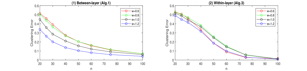
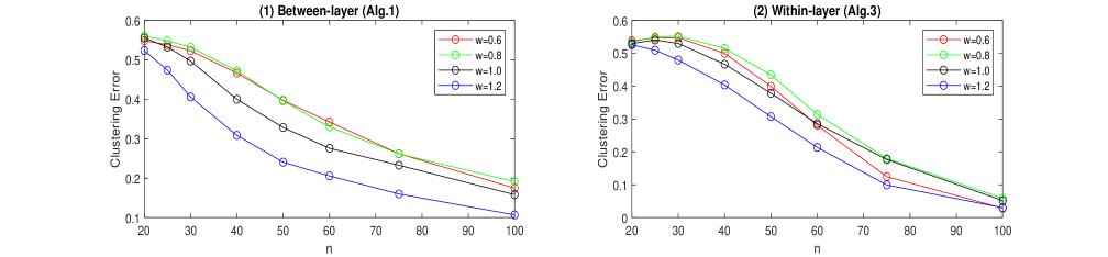
Figure 1: The between-layer clustering error rates of Algorithm 1 (left) and the within-layer error rates of Algorithms 3 (right), averaged over 500 simulation runs, for the DIMPLE model with $c=0,d=0.8$ (top) and $c=0,d=0.5$ (bottom), $L=50$ and $n=20,25,30,40,50,60,75,100$. The entries of $\boldsymbol{B}^{(l)}$, $l\in[L]$, are generated as uniform random numbers between $c$ and $d$. All the non-diagonal entries of those matrices are subsequently multiplied by $w$.

In order to study performances of our methodology for various combinations of parameters, we carry out a limited simulation study with models generated from DIMPLE and DIMPLE-GDPG. We use Algorithm 1 for finding the groups of layers and Algorithms 2 and 3, respectively, for recovering the ambient subspaces in the DIMPLE-GDPG setting, and for finding communities in groups of layers for the DIMPLE model.

To obtain a multilayer network that complies with our assumptions in Section 3.1, we fix $n$, $L$, $M$, $K$, the sparsity parameters $c$ and $d$, the assortativity parameter $w$, and the Dirichlet parameter $\alpha$ used for generating a DIMPLE-GDPG network. We use the multinomial distribution with equal probabilities $1/M$ to assign group memberships to individual networks.

In the case of the DIMPLE model, we generate $K$ communities in each of the groups of layers using the multinomial distribution with equal probabilities $1/K$. In this manner, we obtain community assignment matrices $\mathbf{Z}{{}^{(m)}}$, $m\in[M]$, in each layer $l$ with $c(l)=m$, where $c:[L]\to[M]$ is the layer assignment function. Next, we generate the entries of $\boldsymbol{B}^{(l)}$, $l\in[L]$, as uniform random numbers between $c$ and $d$, and then multiply all the non-diagonal entries of those matrices by $w$. In this manner, if $w<1$ is small, then the network is strongly assortative, i.e., there is a higher probability for nodes in the same community to connect. If $w>1$ is large, then the network is disassortative, i.e., the probability of connection for nodes in different communities is higher than for nodes in the same community. Finally, since entries of matrices $\boldsymbol{B}^{(l)}$ are generated at random, when $w$ is close to one, the networks in all layers are neither assortative or disassortative. After the community assignment matrices $\mathbf{Z}{{}^{(m)}}$ and the block probability matrices $\boldsymbol{B}^{(l)}$ have been obtained, we construct the probability tensor ${\mathcal{P}}$ with layers ${\mathcal{P}}(:,:,l)=\mathbf{Z}{{}^{(m)}}\boldsymbol{B}^{(l)}(\mathbf{Z}{{}^{(m)}})^{T}$, where $m=c(l)$, $l\in[L]$.

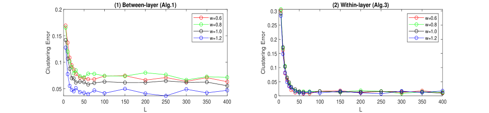
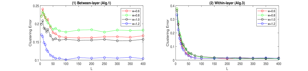
Figure 2: The between-layer clustering error rates of Algorithm 1 (left) and the within-layer error rates of Algorithms 3 (right), averaged over 500 simulation runs, for the DIMPLE model with $c=0,d=0.8$ (top) and $c=0,d=0.5$ (bottom), $n=100$ and $L=5,10,15,20,25,30,40,50,60,75,100,150,200,250,300,350,400$. The entries of $\boldsymbol{B}^{(l)}$, $l\in[L]$, are generated as uniform random numbers between $c$ and $d$. All the non-diagonal entries of those matrices are subsequently multiplied by $w$.

In the case of the DIMPLE-GDPG setting, we obtain matrices $\mathbf{X}^{(m)}\in[0,1]^{n\times K}$, $m\in[M]$, with independent rows, generated using the Dirichlet distribution with parameter $\alpha$. We obtain matrices $\boldsymbol{B}^{(l)}$, in exactly the same manner as in the case of the DIMPLE model and construct ${\mathcal{P}}$ with layers ${\mathcal{P}}(:,:,l)=\mathbf{X}{{}^{(m)}}\boldsymbol{B}^{(l)}(\mathbf{X}{{}^{(m)}})^{T}$, where $m=c(l)$, $l\in[L]$. In this case, the matrices $\mathbf{V}^{(m)}$ are obtained from the SVD $\mathbf{X}^{(m)}=\mathbf{V}^{(m)}\mbox{$\Lambda$}_{X}^{(m)}\mathbf{W}_{X}^{(m)}$ of $\mathbf{X}^{(m)}$. Matrices $\mathbf{Q}^{(l)}$ are defined as $\mathbf{Q}^{(l)}=\mbox{$\Lambda$}_{X}^{(m)}\mathbf{W}_{X}^{(m)}\boldsymbol{B}^{(l)}(\mathbf{W}_{X}^{(m)})^{T}\mbox{$\Lambda$}_{X}^{(m)}$ in (1), $l\in[L]$.

After the probability tensor ${\mathcal{P}}$ is generated, the layers $\mathbf{A}^{(l)}$ of the adjacency tensor ${\mathcal{A}}$ are obtained as symmetric matrices with zero diagonals and independent Bernoulli entries $\mathbf{A}^{(l)}(i,j)$ for $1\leq i<j\leq n$. Subsequently, we use Algorithm 1 for finding the groups of layers for both models, followed by Algorithm 2 for estimating matrices $\mathbf{V}^{(m)}$ in the case of the DIMPLE-GDPG network, or Algorithm 3 for clustering nodes in each group of layers of the network into communities for the DIMPLE model. In both cases, we have two sets of simulations, one with fixed $L$ and varying $n$, another with the fixed $n$ and varying $L$. In all simulations, we set $M=3$ and $K_{m}=3$ for $m=1,2,3$, and study two sparsity scenarios, $c=0$, $d=0.8$ or $c=0$, $d=0.5$, with four values of assortativity parameter $w=0.6,0.8,1.0$ and $1.2$. In all simulations, we set $\alpha=0.1$. We report the average between-layer clustering errors $R_{BL}$ defined in (19), and also the average within-layer clustering error $R_{WL}$ defined in (21) in the case of the DIMPLE setting and the average $\sin\Theta$ distance $R_{S,ave}$ defined in (23) between the true and the estimated subspaces in the case of the DIMPLE-GDPG network. We first present simulations results for the DIMPLE model followed by the study of the DIMPLE-GDPG model.

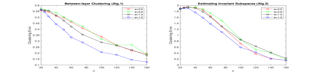
Figure 3: The between-layer clustering error rates of Algorithm 1 (left) and the $\sin\Theta$ distances $R_{S,ave}$ of Algorithms 2 (right), averaged over 100 simulation runs, for the DIMPLE-GDPG model with $\alpha=0.1$, $c=0,d=0.8$ (top) and $c=0,d=0.5$ (bottom), $L=50$ and $n=20,25,30,40,50,60,75,100,120,140,160$. The entries of $\boldsymbol{B}^{(l)}$, $l\in[L]$, are generated as uniform random numbers between $c$ and $d$. All the non-diagonal entries of those matrices are subsequently multiplied by $w$.

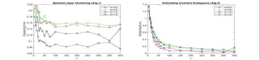
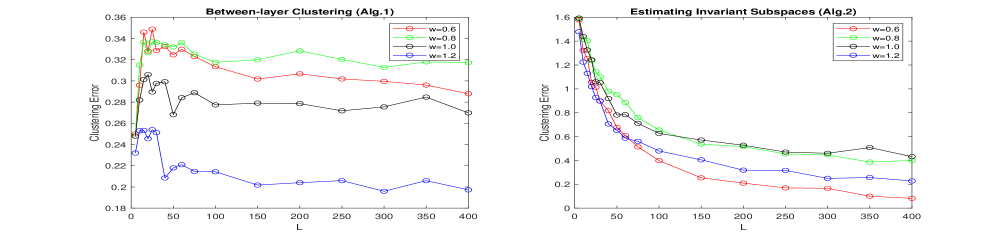
Figure 4: The between-layer clustering error rates of Algorithm 1 (left) and the $\sin\Theta$ distances $R_{S,ave}$ of Algorithms 2 (right), averaged over 100 simulation runs, for the DIMPLE-GDPG model with $\alpha=0.1$, $c=0,d=0.8$ (top) and $c=0,d=0.5$ (bottom), $n=100$ and $L=5,10,15,20,25,30,40,50,60,75,100,150,200,250,300,350,400$. The entries of $\boldsymbol{B}^{(l)}$, $l\in[L]$, are generated as uniform random numbers between $c$ and $d$. All the non-diagonal entries of those matrices are subsequently multiplied by $w$.

Simulations results for the DIMPLE and DIMPLE-GDPG models are summarized in Figures 1–2 and Figures 3–4, respectively. Note that, while the between-layer clustering errors (left panels in Figures 1–4), as well as the within-layer clustering errors (right panels in Figures 1–2) are between 0 and 1, the average errors of estimation of subspaces $R_{S,ave}$ defined in (23) (right panels in Figures 3–4) lie between 0 and $K$, so they are on a different scale.

As it is expected, both estimation and clustering are harder when a network is more sparse, therefore, all errors are smaller when $d=0.8$ (top panels) than when $d=0.5$ (bottom). Figures 1–4 show that the value of the assortativity parameter does not play a significant role in the between-layer clustering. Indeed, as the left panels in all figures show, the smallest between-layer clustering errors occur for $w=1.2$ followed by $w=1.0$. The latter confirms that the difficulty of the between-layer clustering is predominantly controlled by the sparsity of the network. The results are somewhat different for the community detection errors and the subspace estimation errors in, respectively, the DIMPLE and the DIMPLE-GDPG models. Indeed, as the right panels in Figures 1–4 show, the smallest errors occur in the more assortative/disassortative models with $w=0.6$ and $w=1.2$.

One can see from Figures 1 and 3 that, when $n$ grows, all errors decrease. The influence of $L$ on the error rates is more complex. As Theorem 1 implies, the between-layer clustering errors are of the order $(n\rho_{n})^{-1}$ for fixed values of $M$ and $K$. This agrees with the left panels in Figures 2 and 4 where curves exhibit constant behavior for when $L$ grows (small fluctuations are just due to random errors). For the right panels in Figures 2 and 4 this, however, happens only when $L$ is relatively large.

The explanation for such behavior lies in the fact that the between-layer clustering error (corresponding to the left panels in Figures 2 and 4) is of the order $K^{2}\,(n\rho_{n})^{-1}$ and is independent of $L$. On the other hand, for fixed $K$ and $M$, the errors $R_{WL}$ and $R_{S,ave}$ (corresponding to the right panels in, respectively, Figures 2 and 4) are of the order $(n\,\rho_{n})^{-1}+\log n\,(n\,\rho_{n}\,L)^{-1}$. While $L$ is small the second term is dominant but, as $L$ grows. the first term becomes dominant and the errors stop declining as $L$ grows.

5 Application to the Real World Data

In this section, we consider applications of the DIMPLE and the DIMPLE-GDPG models to real-life data, and its comparison with the MMLSBM. Note that the between-layer clustering is carried out by Algorithm 1 for both the DIMPLE and the DIMPLE-GDPG models, so one can decide which of the models to use later in the analysis.

In our examples, the DIMPLE model with its SBM-imposed structures provided better descriptions of the organization of layers in each group than its GDPG-based DIMPLE-GDPG counterpart. Furthermore, we compared our between layer clustering partitions with the ones obtained on the basis of the MMLSBM setting.

5.1 Worldwide Food Trading Network Data

In this subsection, we consider applying our clustering algorithms to the Worldwide Food Trading Networks data collected by the Food and Agriculture Organization of the United Nations. The data have been described in De Domenico et al. (2015), and it is available at https://www.fao.org/faostat/en/#data/TM. The data includes export/import trading volumes among 245 countries for more than 300 food items. These data can be modeled as a multiplex network, in which layers represent different products, nodes are countries, and edges at each layer represent trading relationships of a specific food product among countries. A part of the data set was analyzed in Jing et al. (2021) and Fan et al. (2022).

Similarly to Jing et al. (2021) and Fan et al. (2022), we used data for the year 2010. We start with pre-processing the data by adding the export and import volumes for each pair of countries in each layer of the network, to produce undirected networks that fit in our model. To avoid sparsity, we select 104 countries, whose total trading volumes are higher than the median among all countries. We choose 58 meat/dairy and fruit/vegetable items and constructed a network with 104 nodes and 58 layers.

While pre-processing the data, we observe that global trading patterns are different for the meat/dairy and the fruit/vegetable groups. Specifically, the trading volumes in meat/dairy group are much smaller than the trading volumes in the fruit/vegetable group. For this reason, we choose the thresholds that keep similar sparsity levels for the adjacency matrices. In particular, we set threshold to be equal to 1 unit for the meat/dairy group and 300 units for the fruit/vegetable group, and draw an edge between two nodes (countries) if the total trading volume between them is at or above the threshold.

We scramble the 58 layers and apply Algorithm 1 for the between-layer clustering. Since the food items consist of a meat/dairy and a fruit/vegetable group, we set $M=2$. Due to the fact that there are five food regions (continents) in the world, Asia, America, Europe, Africa and Australia, we start with the number of communities in each layer to be $K=5$. However, the latter leads to an unbalanced community structure, specifically, two communities that consists of only one country. For this reason, after experimenting, we set $K=3$. Results of the between-layer clustering are presented in Figure 5. As it is evident from Figure 5, Algorithm 1 separates the food items into the meat/dairy and the fruit/vegetable groups.

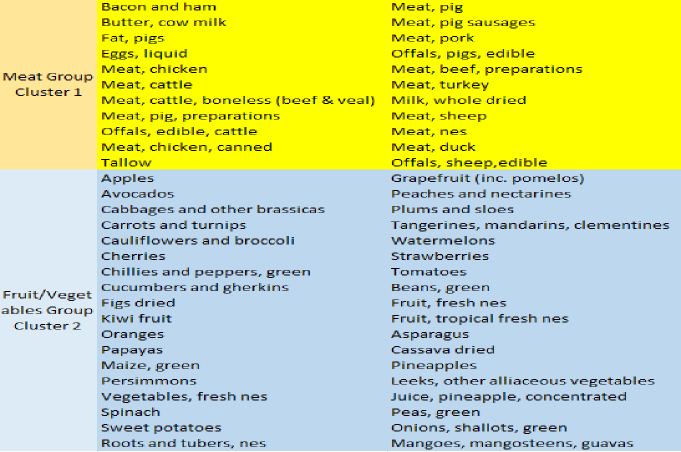
Figure 5: Results of clustering of food networks layers into $M=2$ clusters by Algorithm 1 in the paper

Figure 6: Trading communities for the meat/dairy (top) and the fruit/vegetable (bottom) groups. Left panels: community sizes; right panels: community memberships

Figure 7: Results of clustering of food networks layers into $M=2$ clusters by ALMA algorithm of Fan et al. (2022)

Furthermore, we investigate the communities of countries that form trade clusters in each of the two layers. We use Algorithm 3 in the paper, and exhibit results of the within-layer clustering in Figure 6. The left panels in Figure 6 show the number of nodes (countries) in communities 1,2 and 3 in the meat/dairy and the fruit/vegetable group, respectively. The right panels in Figure 6 project those countries onto the world map. Here, the red color is used for community 1, the yellow color for community 2 and the green color for for community 3. Since we only select 104 countries to be a part of the network, some regions in the map are colored grey.

In order to justify application of the DIMPLE model, we also carry out data analysis assuming that data were generated using the MMLSBM. Specifically, we applied ALMA algorithm of Fan et al. (2022) for the layer clustering with the same parameters $M=2$ and $K=3$. Results are presented in Figure 7. It is easy to notice that ALMA algorithm places some of the meat/dairy items into the fruit/vegetable group. We believe that this is due to the fact that MMLSBM is sensitive to the probabilities of connections rather than connection patterns.

5.2 Global Flights Network Data

Airlines Groups under the DIMPLE-GDPG Model
Group 1		Group 2
China	Hainan Airlines	New Zealand	Air New Zealand
China	Air China	Republic of Korea	Korean Air
China	Sichuan Airlines	Singapore	Singapore Airlines
China	Shenzhen Airlines	Australia	Qantas
China	China Southern Airlines	Vietnam	Vietnam Airlines
China	Shandong Airlines	India	Air India Limited
China	China Eastern Airlines	India	IndiGo Airlines
China	Xiamen Airlines	Australia	Virgin Australia
Japan	Japan Air System	South Africa	South African Airways
Group 3		Indonesia	Garuda Indonesia
Germany	Lufthansa	Republic of Korea	Asiana Airlines
Russia	Ural Airlines	Malaysia	Malaysia Airlines
Switzerland	Swiss International Air Lines	India	Jet Airways
Morocco	Royal Air Maroc	Japan	Japan Airlines
Norway	Norwegian Air Shuttle	Japan	All Nippon Airways
Ireland	Ryanair	Qatar	Qatar Airways
Turkey	Turkish Airlines	Saudi Arabia	Saudi Arabian Airlines
Greece	Aegean Airlines	United Arab Emirates	Emirates
Algeria	Air Algerie	United Arab Emirates	Etihad Airways
Ethiopia	Ethiopian Airlines	Group 4
United Kingdom	Jet2.com	United States	JetBlue Airways
United Kingdom	Flybe	United States	US Airways
Russia	Transaero Airlines	United States	Alaska Airlines
Germany	Condor Flugdienst	United States	Southwest Airlines
Germany	TUIfly	United States	Delta Air Lines
Sweden	Scandinavian Airlines	United States	AirTran Airways
Portugal	TAP Portugal	United States	Spirit Airlines
France	Transavia France	United States	United Airlines
United Kingdom	British Airways	United States	American Airlines
Russia	S7 Airlines	United States	Frontier Airlines
Ireland	Aer Lingus	Canada	Air Canada
Germany	Germanwings	Canada	WestJet
Egypt	Egyptair	Mexico	AeroMexico
Austria	Austrian Airlines	Chile	LAN Airlines
Spain	Iberia Airlines	Brazil	TAM Brazilian Airlines
Germany	Air Berlin	South America	Avianca
Italy	Alitalia	Netherlands	KLM Royal Dutch Airlines
Hungary	Wizz Air	France	Air France
Finland	Finnair
Russia	Aeroflot
France	Air Bourbon
Netherlands	Transavia Holland
United Kingdom	easyJet

Table 1: Airlines Groups obtained using Algorithm 1 with $K=3$ and $M=4$

In this subsection, we applied our clustering algorithms to the Global Flights Network data collected by the OpenFlights. As of June 2014, the OpenFlights Database contains 67663 routes between 3321 airports on 548 airlines spanning the globe. It is available at https://openflights.org/data.html#airport.

These data can be modeled as a multiplex network, in which layers represent different airlines, nodes are airports where airlines depart and land, and edges at each layer represent existing routes of a specific airline company between two airports. To avoid sparsity, we selected 224 airports, where over 150 airline companies have rights to depart and land in. Furthermore, we chose 81 airlines that have at least 240 routes between those airports, constructing a network with 224 nodes and 81 layers.

We scrambled the 81 layers and applied Algorithm 1 for the between-layer clustering. After experimenting with various values of $M$ and $K$, we partitioned the airlines into $M=4$ groups, and used the ambient dimension $K=3$ for each of the groups. Results of the between-layer clustering are presented in Table 1.

Airlines Groups under the MMLSBM
Group 1		Group 2
Japan	Japan Air System	China	Hainan Airlines
China	Sichuan Airlines	China	Air China
China	Shandong Airlines	China	Shenzhen Airlines
China	Xiamen Airlines	China	China Southern Airlines
Republic of Korea	Korean Air	China	China Eastern Airlines
Singapore	Singapore Airlines
Vietnam	Vietnam Airlines	Group 3
India	Air India Limited	France	Air France
United States	US Airways	United States	Delta Air Lines
Australia	Qantas	United States	AirTran Airways
Mexico	AeroMexico	United States	Southwest Airlines
India	IndiGo Airlines	United States	American Airlines
South Africa	South African Airways	Netherlands	KLM Royal Dutch Airlines
Indonesia	Garuda Indonesia	Italy	Alitalia
Republic of Korea	Asiana Airlines
Saudi Arabia	Saudi Arabian Airlines	Group 4
Hong Kong	Cathay Pacific	France	Transavia France
South America	Avianca	France	Air Bourbon
Japan	Japan Airlines	United Kingdom	Jet2.com
Qatar	Qatar Airways	United Kingdom	easyJet
Australia	Virgin Australia	Ireland	Ryanair
Japan	All Nippon Airways
Malaysia	Malaysia Airlines	Group 1: Continuation
India	Jet Airways	Canada	WestJet
United Arab Emirates	Etihad Airways	United Arab Emirates	Emirates
Germany	Lufthansa	Russia	Ural Airlines
Turkey	Pegasus Airlines	Morocco	Royal Air Maroc
Switzerland	Swiss International Airlines	Turkey	Turkish Airlines
Norway	Norwegian Air Shuttle	Ethiopia	Ethiopian Airlines
Greece	Aegean Airlines	Algeria	Air Algerie
United Kingdom	Flybe	Germany	Condor Flugdienst
Germany	TUIfly	Sweden	Scandinavian Airlines
Portugal	TAP Portugal	United Kingdom	British Airways
Russia	S7 Airlines	Austria	Austrian Airlines
Ireland	Aer Lingus	Spain	Iberia Airlines
Germany	Germanwings	Russia	Aeroflot
Egypt	Egyptair	Germany	Air Berlin
Hungary	Wizz Air	Russia	Transaero Airlines
Finland	Finnair	United States	Alaska Airlines
Netherlands	Transavia Holland	Brazil	TAM Brazilian Airlines
United States	JetBlue Airways	United States	Spirit Airlines
Chile	LAN Airlines	Canada	Air Canada
New Zealand	Air New Zealand	United States	Frontier Airlines
United States	United Airlines

Table 2: Airlines Groups obtained using ALMA algorithm of Fan et al. (2022) with $K=3$ and $M=4$

We also partitioned airports in each of the groups of airlines into communities. Results are presented in Figure 8.

Figure 8: Communities for the four airlines groups. Group 1: airlines originated in China. Group 2: airlines originated in Asia, Australia,New Zealand, and Gulf States. Group 3: airlines originated in Europe and North Africa. Group 4: airlines originated in North or South America.

It is easy to see that in Table 1, the airlines are naturally grouped by geographical areas from where the flights are originated. Group 1 is constituted by Chinese airline and one Japanese airline which has flights predominantly in Far East. Group 2 consists of airlines that belong to countries in Asia, such as India, Japan, South Korea and Vietnam, Australia and New Zealand, and few big airlines in Gulf States (Saudi Arabia, United Arab Emirates, Qatar) that have a large number of flights to both Asia and Australia. Group 3 is formed by airlines originated from Europe and North Africa while Group 4 is comprised of airlines that fly in or from North or South America. Not surprisingly, this group includes two big European airlines, KLM and Air France, since those airlines are members of the SkyTeam alliance and share many flights originated in USA with Delta airlines.

We also analyzed the airline data under the assumption that they follow the MMLSBM. To this end, we applied ALMA algorithm of Fan et al. (2022) for the layer clustering, with the same parameters $M=4$ and $K=3$. Results are presented in Table 2. It is easy to see that while the DIMPLE model ensures a logical geography-based partition of the airlines, the MMLSBM does not. Indeed, the MMLSBM lumps almost all airlines into Group 1, placing few Chinese airlines into Group 2, few United States owned airlines together with Air France, Alitalia and KLM into Group 3, and Ryanair (Ireland), Transavia and Air Bourbon (France), easyJet and Jet2.com (United Kingdom) into Group 4. On the contrary, Algorithm 1 associated with the DIMPLE model delivers four balanced (similar in size) groups. This is due to the fact that MMLSBM groups airlines by the volume of operation rather than the structure of roots.

6 Discussion

In this paper, we introduce the GDPG-equipped DIMPLE-GDPG multiplex network model where layers can be partitioned into groups with similar ambient subspace structures while the matrices of connections probabilities can be all different. In the common case when each layer follows the SBM, the latter reduces to the DIMPLE model, where community affiliations are common for each group of layers while the matrices of block connection probabilities vary from one layer to another. The DIMPLE-GDPG model generalizes the COmmon Subspace Independent Edge (COSIE) random graph model of Arroyo et al. (2021) and Zheng and Tang (2022), while the DIMPLE model generalizes a multitude of the SBM-equipped multiplex network settings. Specifically, it includes, as its particular cases, the Mixture MultiLayer Stochastic Block Model (MMLSBM) of Stanley et al. (2016), Jing et al. (2021) and Fan et al. (2022), and the multitude of papers that assume that communities persist in all layers of the network (see, e.g., Bhattacharyya and Chatterjee (2020), Lei and Lin (2021), Lei et al. (2019), Paul and Chen (2016), Paul and Chen (2020)).

Our real data examples in Section 5 show that our models deliver more understandable description of data than the MMLSBM, due to the flexibility of the DIMPLE and DIMPLE-GDPG models.

If $M=1$, the DIMPLE-GDPG reduces to COSIE model, and we believe that our paper provides some improvements due to employment of a different algorithm for the matrix $\mathbf{V}$ estimation. Indeed, Arroyo et al. (2021) showed that

$${\mathbb{E}}\left\|\sin\Theta(\widehat{\mathbf{V}},\mathbf{V})\right\|\leq C\left[\frac{K^{3/2}}{\sqrt{n\,\rho_{n}\,L}}+\frac{K^{5/2}}{n\,\rho_{n}}\right],$$ (45)

while Zheng and Tang (2022), who use a different technique for recovery of $\mathbf{V}$, state that, with high probability, $\|\sin\Theta(\widehat{\mathbf{V}},\mathbf{V})\|_{2\to\infty}\leq C\,Kn^{-1}\,\sqrt{\log n}/\sqrt{\rho_{n}}$. The latter leads to $\|\sin\Theta(\widehat{\mathbf{V}},\mathbf{V})\|_{F}\leq C\,K\,\sqrt{(n\rho_{n})^{-1}\,\log n}$. Thus, the upper bound (45) is similar to our upper bound (42), which is derived for the (larger) Frobenius norm and holds not only in expectation but with the high probability. The upper bound of Zheng and Tang (2022) is larger (if one uses the Frobenius norm) and, in addition, does not decline when $L$ grows.

As our theory (Theorems 1 and 2, and also Corollary 1) the simulation results imply, when $K$ and $M$ are fixed constants, the clustering precision in both algorithms cease to decrease for a given number of nodes $n$ when $L$ grows:

$$R_{BL}\lesssim C\rho_{n}^{-1}n^{-1},\quad R_{S,max}\asymp R_{S,ave}\asymp R_{WL}\lesssim C\left(\rho_{n}^{-1}n^{-1}+n^{-1}\,L^{-1}\,\rho_{n}^{-1}\,\log n\right)$$

We believe that this is not caused by the deficiency of our methodology but is rather due to the fact, that the number of parameters in the model grows linearly in $L$ for a fixed $n$. Indeed, even in the case of the simplest, SBM-based DIMPLE model, the total number of independent parameters in the model is $O(K^{2}L+Mn\log K+L\log M)$, since we have $L$ matrices $\mathbf{B}^{(l)}$, $M$ clustering matrices for the SBMs in the groups of layers, and a clustering matrix of the layers, while the total number of observations is $O(n^{2}L)$. The latter implies that, while for small values of $L$, the term $(Mn\log K)/(n^{2}L)$ may dominate the error, eventually, as $L$ grows, the term $L(K^{2}+\log M)/(n^{2}L)$ becomes larger for a fixed $n$.

Incidentally, we observe that a similar phenomenon holds in the MMLSBM, where the block probability matrices are the same in all layers of each of the groups. While Stanley et al. (2016) does not produce relevant theoretical results, Jing et al. (2021) simply assume that $L\leq n$, which makes the issue of error rates for a growing value of $L$ inconsequential. Similarly, the ALMA clustering error rates in Fan et al. (2022)

$$R_{BL}^{ALMA} \lesssim C\left(\rho_{n}^{-1}\,n^{-2}+\rho_{n}^{-2}\,n^{-2}\,[\min(n,L)]^{-1}\right),$$

$$R_{WL}^{ALMA} \lesssim C\left(n^{-1}\,L^{-1}\,\rho_{n}^{-1}+\rho_{n}^{-1}\,n^{-2}+\rho_{n}^{-2}\,n^{-2}\,[\min(n,L)]^{-1}\right),$$

imply that, for given $n$ and $\rho_{n}$, as $L$ grows, the clustering errors flatten.

Our simulation study also exhibit similar dynamics. In particular, the between-layer clustering errors flatten when $n$ is fixed and $L$ grows, while the errors of subspace estimation and of the within-layer clustering, for a fixed $n$, decrease initially and then stop decreasing as $L$ become larger and larger.

We remark that, unlike the ALMA methodology in Fan et al. (2022) or the TWIST algorithm in Jing et al. (2021), all three algorithms in this paper are not iterative. It is known, that if one needs to recover a low rank tensor, then the power iterations can improve precision guarantees. This has been shown in the context of estimation of a low rank tensor in, e.g., Zhang and Xia (2018a), and in the context of the clustering in the tensor block model in Han et al. (2021). While both ALMA and TWIST are designed for the MMLSBM, which results in a low rank probability tensor, the DIMPLE model does not lead to a low rank probability tensor. Therefore, it is not clear whether iterative techniques are advantageous in the DIMPLE setting. Our very limited experimentation with iterative algorithms did not lead to significant improvement of clustering precision. Investigation of this issue is a matter of future research.

7 Appendix: proofs and additional simulations

7.1 Proof of Theorem 1

Use notations of the paper, note that

$$\left\|\widehat{\mathbf{U}}_{A,l}(\widehat{\mathbf{U}}_{A,l})^{T}-\mathbf{U}_{P,l}(\mathbf{U}_{P,l})^{T}\right\|^{2}_{F}=2\,\left\|\sin\mbox{$\Theta$}(\mathbf{U}_{P,l},\widehat{\mathbf{U}}_{A,l})\right\|^{2}_{F}$$

where $\widehat{\mathbf{U}}_{A,l}$ and $\mathbf{U}_{P,l}$ are defined in (13) and (9), respectively. By Davis-Kahan Theorem,

$$\left\|\widehat{\mathbf{U}}_{A,l}(\widehat{\mathbf{U}}_{A,l})^{T}-\mathbf{U}_{P,l}(\mathbf{U}_{P,l})^{T}\right\|_{F}\leq\frac{2\,\sqrt{K_{m}}\left\|\mathbf{A}^{(l)}-\mathbf{P}^{(l)}\right\|}{\sigma_{K_{m}}(\mathbf{P}^{(l)})},\quad m=c(l)$$

By Theorem 5.2 of Lei and Rinaldo (2015), if $n\rho_{n}\geq C_{\rho}\log n$, then, for any $\tau>0$, there exists a constant $C_{\tau}$, such that

$${\mathbb{P}}\left\{\|\mathbf{A}^{(l)}-\mathbf{P}^{(l)}\|\leq C_{\tau}\sqrt{n\rho_{n}}\right\}\geq 1-n^{-\tau}$$

Then

$${\mathbb{P}}\left\{\max_{l\in[L]}\ \|\mathbf{A}^{(l)}-\mathbf{P}^{(l)}\|\leq C_{\tau}\sqrt{n\rho_{n}}\right\}\geq 1-Ln^{-\tau}$$

In order to construct a lower bound for $\sigma_{K_{m}}(\mathbf{P}^{(l)})$, note that under Assumptions A1–A6, one has

$$\sigma_{K_{m}}(\mathbf{P}^{(l)})=\sigma_{K_{m}}(\mathbf{Q}^{(l)})\geq C_{\lambda}\,K_{m}^{-1/2}\,\|\mathbf{Q}^{(l)}\|\geq\underline{c}_{\rho}C_{\lambda}\,K^{-1/2}\,\rho_{n}\,\|\mathbf{P}_{0}^{(l)}\|\geq\underline{c}_{\rho}C_{\lambda}C_{0,P}\,n\,\rho_{n}\,K^{-1}$$ (46)

Combining the formulas and taking into account that

$$\|\widehat{\mbox{$\Theta$}}-\mbox{$\Theta$}\|^{2}_{F}\leq L\max_{l\in[L]}\ \left\|\widehat{\mathbf{U}}_{A,l}(\widehat{\mathbf{U}}_{A,l})^{T}-\mathbf{U}_{P,l}(\mathbf{U}_{P,l})^{T}\right\|_{F}^{2},$$

obtain

$${\mathbb{P}}\left\{\left\|\widehat{\mbox{$\Theta$}}-\mbox{$\Theta$}\right\|^{2}_{F}\leq C\,\frac{LK^{3}}{n\rho_{n}}\right\}\geq 1-Ln^{-\tau}$$

Also, by Davis-Kahan Theorem,

$$\|\sin\mbox{$\Theta$}(\widehat{\mbox{${\mathcal{W}}$}},\mbox{${\mathcal{W}}$})\|_{F}\leq\frac{\left\|\widehat{\mbox{$\Theta$}}-\mbox{$\Theta$}\right\|_{F}}{\sigma_{M}(\mbox{$\Theta$})}$$

By formula (35) and (36),

$$\sigma_{M}(\mbox{$\Theta$})\geq\sqrt{\frac{\underline{c}}{\bar{c}}}\,\frac{1}{\kappa_{0}^{2}}\,\left\|\mbox{$\Theta$}\right\|\geq\sqrt{\frac{\underline{c}}{\bar{c}}}\,\frac{1}{\kappa_{0}^{2}}\,\frac{\left\|\mbox{$\Theta$}\right\|_{F}}{\sqrt{M}}\geq\sqrt{\frac{\underline{c}}{\bar{c}}}\,\frac{\sqrt{KL}}{\kappa_{0}^{2}\sqrt{M}}$$

Hence,

$${\mathbb{P}}\left\{\left\|\sin\mbox{$\Theta$}(\widehat{\mbox{${\mathcal{W}}$}},\mbox{${\mathcal{W}}$})\right\|^{2}_{F}\leq\frac{CK^{2}M}{n\rho_{n}}\right\}\geq 1-Ln^{-\tau}$$

Use Lemma C.1 of Lei and Lin (2021):

Lemma 2.

( Lemma C.1 of Lei and Lin (2021)). Let $\mathbf{X}$ be an $m\times d$ matrix with $K$ distinct rows and minimum pairwise Euclidean norm separation $\gamma$. Let $\widehat{\mathbf{X}}$ be another $(m\times d)$ matrix and $(\widehat{\mbox{$\Theta$}},\widehat{\mathbf{Q}})$ be an $(1+\epsilon)$-approximate solution to $K$-means problem with input $X$. Then, the number of errors in $\widehat{\mbox{$\Theta$}}$ as an estimate number of errors in $\widehat{\mbox{$\Theta$}}$ as an estimate of row clusters of $X$ is no larger than $\mathbf{C}_{\epsilon}\left\|\sin\mbox{$\Theta$}(\widehat{\mathbf{X}},\mathbf{X})\right\|^{2}_{F}\gamma^{-2}$, where $\mathbf{C}_{\epsilon}$ depends only on $\epsilon$.

Since the row separation of ${\mathcal{W}}$ is at least $1/\sqrt{L_{m}}\geq\sqrt{M}/(\bar{c}\sqrt{L})$, the number of errors is bounded above by $CK^{2}L\,(n\rho_{n})^{-1}$, with probability at least $1-Ln^{-\tau}$. The latter, in combination with (31), implies (38).

7.2 Proof of Theorem 2

The proof requires the following lemma.

Lemma 3.

Let $\mathbf{W}$ and $\widehat{\mathbf{W}}$ be defined as in (11) and (16), respectively. Let assumptions of Theorem 2 hold. Then, on the set $\Omega$, with ${\mathbb{P}}(\Omega)\geq 1-L\,n^{-\tau}$, on which (38) holds, one has

$$0.5\,L_{m}^{-1}\leq\widehat{L}_{m}\leq 2\,L_{m}^{-1},\quad m\in[M]$$ (47)

$$|\widehat{L}_{m}^{-1/2}-L_{m}^{-1/2}|\leq C(n\rho_{n}\sqrt{L_{m}})^{-1}\,MK^{2},\quad m\in[M]$$ (48)

$$\min_{\mathscr{P}\in\mathfrak{F}(M)}\ \|\widehat{\mathbf{W}}-\mathbf{W}\,\mathscr{P}\|^{2}_{F}\leq C(n\rho_{n})^{-1}\,MK^{2}$$ (49)

Consider tensors ${\mathcal{G}}\in{\mathbb{R}}^{n\times n\times L}$ and ${\mathcal{H}}={\mathcal{G}}\times_{3}\mathbf{W}^{T}\in{\mathbb{R}}^{n\times n\times M}$ with layers, respectively, $\mathbf{G}^{(l)}={\mathcal{G}}(:,:,l)$ and $\mathbf{H}^{(m)}={\mathcal{H}}(:,:,m)$ of the forms

$$\mathbf{G}^{(l)}=(\mathbf{P}^{(l)})^{2},\quad\mathbf{H}^{(m)}=L_{m}^{-1/2}\,\sum_{c(l)=m}\,\mathbf{G}^{(l)},\quad l\in[L],\ m\in[M]$$ (50)

In order to assess $R_{S,max}$ and $R_{S,ave}$, one needs to examine the spectral structure of matrices $\mathbf{H}^{(m)}$ and their deviation from the sample-based versions $\widehat{\mathbf{H}}^{(m)}=\widehat{{\mathcal{H}}}(:,:,m)$. We start with the first task.

It follows from (7) and (8) that

$$\mathbf{H}^{(m)}=\mathbf{V}^{(m)}\,\overline{\mathbf{Q}}^{(m)}\,(\mathbf{V}^{(m)})^{T}\quad\mbox{with}\quad\overline{\mathbf{Q}}^{(m)}=L_{m}^{-1/2}\,\sum_{c(l)=m}\,\left(\mathbf{Q}^{(l)}\right)^{2}$$ (51)

Here, by (7), one has $(\mathbf{Q}^{(l)})^{2}=\mathbf{O}_{Q}^{(l)}(\mathbf{S}_{Q}^{(l)})^{2}(\mathbf{O}_{Q}^{(l)})^{T}$, so that all eigenvalues of $(\mathbf{Q}^{(l)})^{2}$ are positive. Applying the Theorem in Complement 10.1.2 on page 327 of Rao and Rao (1998) and Assumptions A1–A6, obtain

$$\sigma_{K_{m}}(\mathbf{H}^{(m)}) =\sigma_{K_{m}}\left(\overline{\mathbf{Q}}^{(m)}\right)\geq L_{m}^{-1/2}\,\sum_{c(l)=m}\sigma_{K_{m}}\left((\mathbf{Q}^{(l)})^{2}\right)$$

$$\geq C_{\lambda}^{2}\,L_{m}^{-1/2}\,K_{m}^{-1}\,\sum_{c(l)=m}\|\mathbf{Q}^{(l)}\|^{2}_{F}\geq C_{\lambda}^{2}\,L_{m}^{-1/2}\,K^{-1}\,\sum_{c(l)=m}\rho_{n,l}^{2}\,\|\mathbf{P}_{0}^{(l)}\|^{2}_{F}$$

$$\geq C_{\lambda}^{2}\,\underline{c}_{\rho}^{2}\,C_{0,P}^{2}\,L_{m}^{-1/2}\,K^{-2}\,n^{2}\ \rho_{n}^{2}\,L_{m}$$

so that

$$\sigma_{K_{m}}\left(\mathbf{H}^{(m)}\right)\geq C\,(K^{2}\sqrt{M})^{-1}\,n^{2}\ \rho_{n}^{2}\,\sqrt{L}$$ (52)

Using Davis-Kahan theorem, Lemma 1 of Cai and Zhang (2018b) and formula (52), obtain

$$\left\|\sin\Theta\left(\widehat{\mathbf{V}}^{(m)},\mathbf{V}^{(m)}\right)\right\|_{F}\leq\frac{2\,\sqrt{2K_{m}}\,\|\widehat{\mathbf{H}}^{(m)}-\mathbf{H}^{(m)}\|}{\sigma_{K_{m}}(\mathbf{H}^{(m)})}\leq\frac{C\,K^{5/2}\,M^{1/2}\,\|\widehat{\mathbf{H}}^{(m)}-\mathbf{H}^{(m)}\|}{n^{2}\,\rho_{n}^{2}\,\sqrt{L}}$$ (53)

Recall that $\mathbf{H}^{(m)}=[{\mathcal{G}}\times_{3}\mathbf{W}^{T}](:,:,m)$ and $\widehat{\mathbf{H}}^{(m)}=[\widehat{{\mathcal{G}}}\times_{3}\widehat{\mathbf{W}}^{T}](:,:,m)$. Denote

$$\overline{\mathbf{G}}^{(m)}=\displaystyle\sum_{c(l)=m}\mathbf{G}^{(l)}=\sqrt{L_{m}}\,\mathbf{H}^{(m)},\quad\overline{\widehat{\mathbf{G}}}^{(m)}=\sqrt{L_{m}}\,\left[\widehat{{\mathcal{G}}}\times_{3}\mathbf{W}^{T}\right](:,:,m)=\displaystyle\sum_{c(l)=m}\widehat{\mathbf{G}}^{(l)}$$ (54)

Observe that

$$\|\widehat{\mathbf{H}}^{(m)}-\mathbf{H}^{(m)}\|\leq\Delta_{1}^{(m)}+\Delta_{2}^{(m)},\quad\sum_{m=1}^{M}\|\widehat{\mathbf{H}}^{(m)}-\mathbf{H}^{(m)}\|^{2}\leq 2(\Delta_{1}+\Delta_{2})$$ (55)

where

$$\Delta_{1}^{(m)} =L_{m}^{-1/2}\left\|\overline{\widehat{\mathbf{G}}}^{(m)}-\overline{\mathbf{G}}^{(m)}\right\|,\quad\Delta_{2}^{(m)}=\left\|[\widehat{{\mathcal{G}}}\times_{3}(\widehat{\mathbf{W}}-\mathbf{W})^{T}](:,:,m)\right\|,$$

$$\Delta_{i} =\sum(\Delta_{i}^{(m)})^{2},\quad i=1,2$$

To upper-bound $\Delta_{1}^{(m)}$ and $\Delta_{2}^{(m)}$, we use the following lemma that modifies upper bounds in Theorem 3 of Lei and Lin (2021) in the absence of the sparsity assumption $\rho_{n}n\leq C$:

Lemma 4.

Let Assumptions A1–A6 hold, $\mathbf{G}^{(l)}=(\mathbf{P}^{(l)})^{2}$ and $\widehat{\mathbf{G}}^{(l)}=(\mathbf{A}^{(l)})^{2}-{\rm diag}(\mathbf{A}^{(l)}\mathbf{1})$, where $c(l)=m$, $l\in[\widetilde{L}]$. Let

$$\mathbf{G}=\sum_{l=1}^{\widetilde{L}}\,\mathbf{G}^{(l)},\quad\widehat{\mathbf{G}}=\sum_{l=1}^{\widetilde{L}}\,\widehat{\mathbf{G}}^{(l)}$$

Then, for any $\tau>0$, there exists a constant $C$ that depends only on constants in Assumptions A1–A6, and a constant $\widetilde{C}_{\tau,\epsilon}$ which depends only on $\tau$ and $\epsilon$, such that one has

$${\mathbb{P}}\left\{\|\widehat{\mathbf{G}}-\mathbf{G}\|\leq C\,\left[\rho_{n}^{3/2}n^{3/2}\sqrt{\widetilde{L}\,\log(\widetilde{L}+n)}+\rho_{n}^{2}n\widetilde{L}\right]\right\}\geq 1-\widetilde{C}_{\tau,\epsilon}n^{1-\tau}$$ (56)

Applying Lemma 4 with $\widetilde{L}=L_{m}$ and taking into account that, by assumption (31), one has $\log n\leq\log(L+n)\leq(1+\tau_{0})\log n$, obtain that, with probability at least $1-\widetilde{C}_{\tau,\epsilon}n^{1-\tau}$, one has $\Delta_{1}^{(m)}\leq\widetilde{C}[\rho_{n}^{3/2}n^{3/2}\sqrt{\log n}+\rho_{n}^{2}\,n\sqrt{L_{m}}]$. Therefore,

$${\mathbb{P}}\left\{\max_{m\in[M]}\Delta_{1}^{(m)}\leq C\left[\rho_{n}^{3/2}n^{3/2}\sqrt{\log n}+\rho_{n}^{2}\,n\sqrt{L/M}\right]\right\}\geq 1-\widetilde{C}_{\tau,\epsilon}\,M\,n^{1-\tau}$$ (57)

and $\Delta_{1}\leq C[\rho_{n}^{3/2}n^{3/2}\,M\sqrt{\log n}+\rho_{n}^{2}\,n\sqrt{L\,M}]$ with the same probability.

In the case of $\Delta_{2}^{(m)}$, we start with an upper bound for $\Delta_{2}$. Note that, by Cauchy inequality and Lemma 3, with probability at least $1-L\,n^{-\tau}$, one has

$$\Delta_{2} = \sum_{m=1}^{M}\left\|\sum_{l=1}^{L}\widehat{\mathbf{G}}^{(l)}(\widehat{\mathbf{W}}_{l,m}-\mathbf{W}_{l,m})\right\|^{2}\leq\sum_{m=1}^{M}\left[\sum_{l=1}^{L}\left\|\widehat{\mathbf{G}}^{(l)}\right\|\,\left|\widehat{\mathbf{W}}_{l,m}-\mathbf{W}_{l,m}\right|\right]^{2}$$ (58)

$$\leq \|\widehat{\mathbf{W}}-\mathbf{W}\|_{F}^{2}\ \sum_{l=1}^{L}\|\widehat{\mathbf{G}}^{(l)}\|^{2}\leq C(n\rho_{n})^{-1}\,M\,K^{2}\ \sum_{l=1}^{L}\|\widehat{\mathbf{G}}^{(l)}\|^{2}$$

In order to obtain an upper bound for the sum of $\|\widehat{\mathbf{G}}^{(l)}\|^{2}$, use Lemma 4 with $\widetilde{L}=1$. Derive

$${\mathbb{P}}\left\{\max_{l\in[L]}\ \|\widehat{\mathbf{G}}^{(l)}-\mathbf{G}^{(l)}\|^{2}\leq C\,\left[\rho_{n}^{3}n^{3}\,\log n+\rho_{n}^{4}n^{2}\right]\right\}\geq 1-\widetilde{C}_{\tau,\epsilon}L\,n^{1-\tau}$$

On the other hand,

$$\|\mathbf{G}^{(l)}\|\leq\|\mathbf{P}^{(l)}\|^{2}\leq C_{\lambda}^{-2}\,[\sigma_{K_{m}}(\mathbf{P}^{(l)})]^{2}\leq C_{\lambda}^{-2}\,K_{m}^{-1}\|\mathbf{P}^{(l)}\|^{2}_{F}\leq C_{\lambda}^{-2}\,C_{K}^{-1}\,K^{-1}(n\rho_{n})^{2}$$

Since $\|\widehat{\mathbf{G}}^{(l)}\|\leq\|\mathbf{G}^{(l)}\|+\|\widehat{\mathbf{G}}^{(l)}-\mathbf{G}^{(l)}\|$, with probability at least $1-\widetilde{C}_{\tau,\epsilon}L\,n^{1-\tau}$, obtain

$$\max_{l\in[L]}\ \|\widehat{\mathbf{G}}^{(l)}\|^{2}\leq C\left(K^{-2}\,n^{4}\,\rho_{n}^{4}+\rho_{n}^{3}n^{3}\,\log n+\rho_{n}^{4}n^{2}\right)\leq CK^{-2}\,n^{4}\,\rho_{n}^{4}\left(1+(n\rho_{n})^{-1}\,K^{2}\log n\right)$$

Plugging the latter upper bound into (58), obtain

$${\mathbb{P}}\left\{\Delta_{2}\leq Cn^{3}\rho_{n}^{3}\,L\,M\,\left(1+(n\rho_{n})^{-1}\,K^{2}\log n\right)\right\}\geq 1-\widetilde{C}_{\tau,\epsilon}\,L\,n^{1-\tau}$$ (59)

To complete the proof, combine formulas (53), (55), (57) and (59) take into account that $\Delta_{2}^{(m)}\leq\sqrt{\Delta_{2}}$ for any $m\in[M]$.

7.3 Proof of Corollary 1

To find the clustering errors for each group of clusters, we again use Lemma 2 which yields that the number of clustering errors in the layer $m\in[M]$ is bounded above by $\mathbf{C}_{\epsilon}\left\|\sin\mbox{$\Theta$}(\widehat{\mathbf{V}}^{(m)},\mathbf{V}^{(m)})\right\|^{2}_{F}\gamma_{m}^{-2}$, where $\gamma_{m}$ is the minimum pairwise Euclidean norm separation between rows of matrix $\mathbf{V}^{(m)}$. It is easy to see that under Assumptions A1–A6, one has

$$\gamma_{m}^{2}\geq 2\min(n_{k,m}^{-1})\geq 2\,C_{K}\,K/(\bar{c}\,n),$$ (60)

so that the total number of errors is bounded above by $C\,M\,K^{-1}\,n\,R_{S,ave}$ where $R_{S,ave}$ is given by (41). Then, the average within layer clustering error is bounded above by $K^{-1}\,R_{S,ave}$, which completes the proof.

7.4 Proof of supplementary lemmas

Proof of Lemma 1 Note that, due to the structure of the tensor ${\mathcal{B}}$, for some $s>0$, one has $\sigma_{\min}(\overline{\mathbf{R}})=\sigma_{\max}(\overline{\mathbf{R}})=s$, so that

$$\sigma_{1}(\mathbf{F})\leq\sigma_{1}^{2}(\overline{\mathbf{D}})\,s\,\sqrt{\max_{m\in[M]}L_{m}},\quad\sigma_{M}(\mathbf{F})\geq\sigma_{M}^{2}(\overline{\mathbf{D}})\,s\,\sqrt{\min_{m\in[M]}L_{m}}.$$

Then, by Assumptions A1 and A4, $\sigma_{1}^{2}(\mathbf{F})\leq\kappa_{0}^{4}\sigma_{M}^{2}(\mathbf{F})\bar{c}/\underline{c}$. Therefore, the first inequality in (36) holds. To prove the second inequality, observe that

$$\|\mbox{$\Theta$}\|^{2}_{F}=\mbox{Tr}(\mathbf{F}\mathbf{F}^{T}(\overline{\mathbf{U}}^{T}\overline{\mathbf{U}}\otimes\overline{\mathbf{U}}^{T}\overline{\mathbf{U}}))=\|\mathbf{F}\|^{2}_{F}$$

and, on the other hand,

$$\|\mbox{$\Theta$}\|^{2}_{F}=\sum_{l=1}^{L}\|\mathbf{U}_{P,l}(\mathbf{U}_{P,l})^{T}\|^{2}_{F}=\sum_{m=1}^{M}L_{m}\|\mathbf{V}^{(m)}(\mathbf{V}^{(m)})^{T}\|^{2}_{F}=\sum_{m=1}^{M}L_{m}K_{m}\geq C_{K}KL,$$ (61)

which together complete the proof.

Proof of Lemma 3 Note that, for $m\in[M]$, $|\widehat{L}_{m}-L_{m}|\leq LR_{BL}\leq C(n\rho_{n})^{-1}\,L\,K^{2}$. Then,

$$\left|\frac{1}{\widehat{L}_{m}}-\frac{1}{L_{m}}\right|=\frac{|\widehat{L}_{m}-L_{m}|}{\widehat{L}_{m}\,L_{m}}\leq\frac{CMK^{2}}{n\rho_{n}}\ \frac{1}{\widehat{L}_{m}}$$

Then, due to assumption (39), the coefficient in front of $\widehat{L}_{m}^{-1}$ is bounded by $1/2$ and, hence, (47) holds. Inequality (48) follows directly from the upper bound on $|\widehat{L}_{m}-L_{m}|$ and (47).

To prove (49), recall that formulas (11) and (16) imply that

$$\|\widehat{\mathbf{W}}-\mathbf{W}\|^{2}_{F} \leq \left\|\widehat{\mathbf{C}}(\widehat{\mathbf{D}}_{\hat{c}})^{-1/2}-\mathbf{C}(\mathbf{D}_{c})^{-1/2}\right\|^{2}_{F}$$

$$\leq 2\left\|\widehat{\mathbf{C}}(\widehat{\mathbf{D}}_{\hat{c}})^{-1/2}\right\|^{2}\ \left\|\mathbf{I}_{M}-(\widehat{\mathbf{D}}_{\hat{c}})^{1/2}(\mathbf{D}_{c})^{-1/2}\right\|^{2}_{F}+2\left\|\widehat{\mathbf{C}}-\mathbf{C}\right\|^{2}_{F}\ \left\|(\mathbf{D}_{c})^{-1/2}\right\|^{2}$$

where $\mathbf{D}_{c}={\rm diag}(L_{1},...,L_{M})$ and $\widehat{\mathbf{D}}_{\hat{c}}={\rm diag}(\widehat{L}_{1},...,\widehat{L}_{M})$. It is easy to see that $\|\widehat{\mathbf{C}}(\widehat{\mathbf{D}}_{\hat{c}})^{-1/2}\|=1$ in (7.4), and that, by Assumption A1, $\|(\mathbf{D}_{c})^{-1/2}\|^{2}\leq(\min L_{m})^{-1}\leq M/(\underline{c}\,L)$. Also, $\|\widehat{\mathbf{C}}-\mathbf{C}\|^{2}_{F}\leq 2L\ R_{BL}$, and

$$\|\mathbf{I}_{M} -(\widehat{\mathbf{D}}_{\hat{c}})^{1/2}(\mathbf{D}_{c})^{-1/2}\|^{2}_{F}=\mbox{Tr}(\mathbf{I}_{M}+\widehat{\mathbf{D}}_{\hat{c}}\mathbf{D}_{c}^{-1}-2(\widehat{\mathbf{D}}_{\hat{c}})^{1/2}(\mathbf{D}_{c})^{-1/2})$$

$$=\sum_{m=1}^{M}\frac{\left(\widehat{L}_{m}^{1/2}-L_{m}^{1/2}\right)^{2}}{L_{m}}\leq\sum_{m=1}^{M}\frac{|\widehat{L}_{m}-L_{m}|}{L_{m}}\leq\frac{M}{\underline{c}\,L}\ \sum_{m=1}^{M}|\widehat{L}_{m}-L_{m}|,$$

due to Assumption A1, and $(\sqrt{a}-\sqrt{b})^{2}\leq|a-b|$ for any $a,b>0$. Since $\sum|\widehat{L}_{m}-L_{m}|$ is dominated by the number of clustering errors $L\,R_{BL}$, plugging all components into (7.4), obtain (49).

Proof of Lemma 4 Let $\mathbf{X}^{(l)}=\mathbf{A}^{(l)}-\mathbf{P}^{(l)}$, $l=1,...,\widetilde{L}$. With some abuse of notations, for any square matrix $\mathbf{Q}$, let ${\rm diag}(\mathbf{Q})$ be the diagonal matrix which diagonal entries are equal to the diagonal entries of $\mathbf{Q}$, while for any vector $\mathbf{q}$, let ${\rm diag}(\mathbf{q})$ be the diagonal matrix with the vector $\mathbf{q}$ on the diagonal. Then, $\widehat{\mathbf{G}}-\mathbf{G}=\mathbf{S}_{1}+\mathbf{S}_{2}+\mathbf{S}_{3}$ where

$$\mathbf{S}_{1}=\sum_{l=1}^{\widetilde{L}}\,(\mathbf{P}^{(l)}\mathbf{X}^{(l)}+\mathbf{X}^{(l)}\mathbf{P}^{(l)}),\quad\mathbf{S}_{2}=\sum_{l=1}^{\widetilde{L}}\,\left[(\mathbf{X}^{(l)})^{2}-{\rm diag}((\mathbf{X}^{(l)})^{2})\right],$$

$$\mathbf{S}_{3}=\sum_{l=1}^{\widetilde{L}}\,\left[{\rm diag}((\mathbf{X}^{(l)})^{2})-{\rm diag}(\mathbf{A}^{(l)}\mathbf{1})\right]$$

Therefore, $\|\widehat{\mathbf{G}}-\mathbf{G}\|^{2}\leq 3(\|\mathbf{S}_{1}\|^{2}+\|\mathbf{S}_{2}\|^{2}+\|\mathbf{S}_{3}\|^{2})$.

To bound above $\|\mathbf{S}_{1}\|^{2}$, $\|\mathbf{S}_{2}\|^{2}$ and $\|\mathbf{S}_{3}\|^{2}$, apply Theorems 2 and 3 of Lei and Lin (2021) with $v_{1}=v_{2}=2\bar{c}_{\rho}\rho_{n}$, $R_{1}=R_{2}=R_{2}^{\prime}=1$ and $v_{2}^{\prime}=2\bar{c}_{\rho}^{2}\rho_{n}^{2}$. Using Theorems 2 with $m=r=n$ and $t^{2}=\tau\bar{c}_{\rho}^{2}C_{\rho}\rho_{n}^{3}n^{3}\widetilde{L}\log n$, obtain

$${\mathbb{P}}\left\{\|\mathbf{S}_{1}\|^{2}\leq\widetilde{C}\rho_{n}^{3}n^{3}\widetilde{L}\log n\right\}\geq 1-4n^{1-\tau}$$

The first part of Theorem 3 yields that, due to Assumption A3,

$${\mathbb{P}}\left\{\|\mathbf{S}_{2}\|^{2}\leq\widetilde{C}\rho_{n}^{2}n^{2}\widetilde{L}\log^{2}(n+\widetilde{L})\right\}\geq 1-C(n+\widetilde{L})^{1-\tau}$$

Now, $\|\mathbf{S}_{3}\|\leq\|\mathbf{S}_{3}-{\mathbb{E}}(\mathbf{S}_{3})\|+\displaystyle\max_{i}|({\mathbb{E}}\mathbf{S}_{3})(i,i)|$, since $\mathbf{S}_{3}$ is a diagonal matrix. Applying second part of Theorem 3 with $\sigma_{2}=1$ and $\sigma^{\prime}_{2}=\sqrt{\widetilde{L}n}$, obtain

$${\mathbb{P}}\left\{\|\mathbf{S}_{3}-{\mathbb{E}}(\mathbf{S}_{3})\|^{2}\leq\widetilde{C}\rho_{n}n\widetilde{L}\log^{2}(n+\widetilde{L})\right\}\geq 1-C(n+\widetilde{L})^{1-\tau}$$

Finally,

$$|({\mathbb{E}}\mathbf{S}_{3})(i,i)|=\left|\sum_{l=1}^{\widetilde{L}}\left[{\mathbb{E}}\sum_{j=1}^{n}[\mathbf{X}^{(l)}(i,j)]^{2}-\sum_{j=1}^{n}\mathbf{P}^{(l)}(i,j)\right]\right|=\sum_{l=1}^{\widetilde{L}}\sum_{j=1}^{n}[\mathbf{P}^{(l)}(i,j)]^{2}\leq\rho_{n}^{2}n\widetilde{L},$$

which completes the proof.

7.5 The DIMPLE model versus the MMLSBM

As we have previously mentioned, in this paper we consider the DIMPLE model, which is a more general model than the MMLSBM. Specifically, the MMLSBM has only $M$ types of layers in the tensor and, therefore, results in a low rank tensor. On the other hand, all tensor layers in the DIMPLE model can be different and, therefore, the tensor is not of low rank. In this section, we carry out a limited simulation study, the purpose of which is to convince a reader that, while our algorithms work in the case of the MMLSBM, the algorithms designed for the MMLSBM produce poor results when data are generated according to the DIMPLE models.

In particular, in both scenarios, we first fix $n$, $L$, $M$, $K$ and generate $M$ groups of layers using the multinomial distribution with equal probabilities $1/M$. Similarly, we generate $K$ communities in each of the groups of layers using the multinomial distribution with equal probabilities $1/K$. In this manner, we obtain community assignment matrices $\mathbf{Z}{{}^{(m)}}$, $m=1,...,M$, in each layer $l$ with $c(l)=m$, where $c:[L]\to[M]$ is the layer assignment function. Next, we choose sparsity parameters $c$ and $d$ and assortativity parameter $w$.

Figure 9: The between-layer clustering error rates of Algorithm 1 and Alternative Minimization Algorithm of Fan et al. (2022). Data are generated using DIMPLE model with $L=50$, $c=0$, $d=0.8$ (top) and $c=0$, $d=0.5$ (bottom), and $w=0.7$ (left panel) or $w=1$ (right panel).

Figure 10: The between-layer clustering error rates of Algorithm 1 and Alternative Minimization Algorithm of Fan et al. (2022). Data are generated using DIMPLE model with $L=100$, $c=0$, $d=0.8$ (top) and $c=0$, $d=0.5$ (bottom), $n=20,40,60,80,100,120,140,160$ and $w=0.7$ (left panel) or $w=1$ (right panel).

In order to generate data according to the DIMPLE model, we obtain the entries of $\boldsymbol{B}^{(l)}$, $l=1,...,L$, as uniform random numbers between $c$ and $d$, and then multiply all the non-diagonal entries of those matrices by $w$. Therefore, if $w<1$ is small, then the network is strongly assortative, i.e., there is higher probability for nodes in the same community to connect.

The next four figures present simulation results for $K=5$, $M=3$ and various values of $L$, $n$, $c$, $d$ and $w$. We present only the between layer clustering errors since, in the presence of the assortativity assumption, the within-layer clustering in the MMLSBM and the DIMPLE model can be carried out in a similar way. We compare the performances of Algorithm 1 in this paper with the Alternative Minimization Algorithm (ALMA) of Fan et al. (2022).

As our simulations show, when data are generated according to the DIMPLE model, Algorithm 1 in our paper allows to reliably separate layers of the network into $M$ types, while ALMA fails to do so. The reason for this is that ALMA expects the matrices of probabilities to be identical in those layers, although, in reality, they are not. As a result, when $n$ grows, the clustering errors do not tend to zero but just flatten.

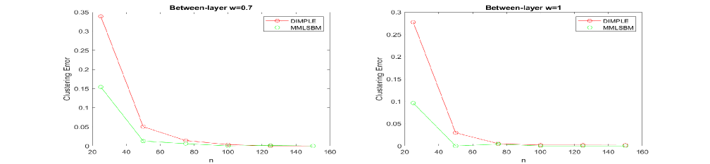
Figure 11: The between-layer clustering error rates of Algorithm 1 and Alternative Minimization Algorithm of Fan et al. (2022). Data are generated using MMLSBM with $L=50$, $c=0$, $d=0.8$ (top) and $c=0$, $d=0.5$ (bottom), $n=20,40,60,80,100,120,140,160$ and $w=0.7$ (left panel) or $w=1$ (right panel).

Next, we generate data according to the MMLSBM. Note that the main difference between the MMLSBM and the DIMPLE model is that in MMLSBM one has only $M$ distinct matrices $\boldsymbol{B}^{(l)}$, since $\boldsymbol{B}^{(l)}=\boldsymbol{B}^{(c(l))}$, $l=1,...,L$. So, in order to generate MMLSBM, we generate $M$ matrices $\boldsymbol{B}^{(m)}$, $m=1,...,M$, and then set $\boldsymbol{B}^{(l)}=\boldsymbol{B}^{(c(l))}$, $l=1,...,L$. Figures 9–12 exhibit results of application of Algorithm 1 and ALMA of Fan et al. (2022) to the generated data sets. As it is expected, for small values of $n$, ALMA of Fan et al. (2022) leads to a better clustering precision. The latter is due to the fact that Algorithm 1 relies on the SVDs of the layers of the adjacency tensor ${\mathcal{A}}$, that are not reliable for small values of $n$. In addition, Algorithm 1 cannot take into account that the probability tensor is of a low rank since this is not true for the DIMPLE model. However, these advantages become less and less significant as $n$ grows. As Figures 9–12 show, both algorithms have similar clustering precision for larger values of $n$, specifically, for $n\geq n_{0}$, where $n_{0}$ is between 60 and 100, depending on a particular simulations setting.

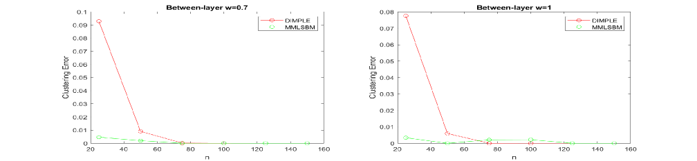
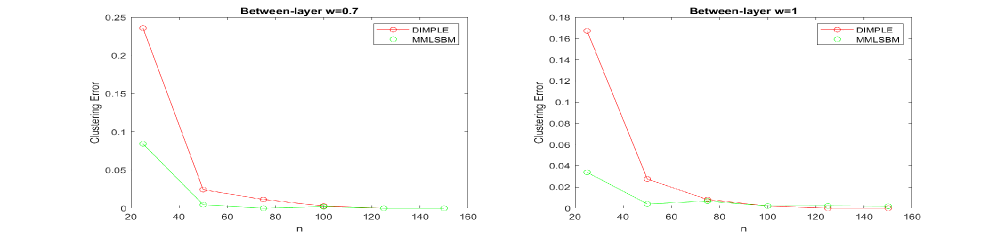
Figure 12: The between-layer clustering error rates of Algorithm 1 and Alternative Minimization Algorithm of Fan et al. (2022). Data are generated using MMLSBM with $L=100$, $c=0$, $d=0.8$ (top) and $c=0$, $d=0.5$ (bottom), and $w=0.7$ (left panel) or $w=1$ (right panel).

References

- Aleta and Moreno (2019) Alberto Aleta and Yamir Moreno. Multilayer networks in a nutshell. Annual Review of Condensed Matter Physics, 10(1):45–62, Mar 2019. doi: 10.1146/annurev-conmatphys-031218-013259. URL http://dx.doi.org/10.1146/annurev-conmatphys-031218-013259.
- Arroyo et al. (2021) Jesus Arroyo, Avanti Athreya, Joshua Cape, Guodong Chen, Carey E. Priebe, and Joshua T. Vogelstein. Inference for multiple heterogeneous networks with a common invariant subspace. Journal of Machine Learning Research, 22(142):1–49, 2021. URL http://jmlr.org/papers/v22/19-558.html.
- Athreya et al. (2018) Avanti Athreya, Donniell E. Fishkind, Minh Tang, Carey E. Priebe, Youngser Park, Joshua T. Vogelstein, Keith Levin, Vince Lyzinski, Yichen Qin, and Daniel L Sussman. Statistical inference on random dot product graphs: a survey. Journal of Machine Learning Research, 18(226):1–92, 2018. URL http://jmlr.org/papers/v18/17-448.html.
- Bhattacharyya and Chatterjee (2020) Sharmodeep Bhattacharyya and Shirshendu Chatterjee. General community detection with optimal recovery conditions for multi-relational sparse networks with dependent layers. ArXiv:2004.03480, 2020.
- Brodka et al. (2018) Piotr Brodka, Anna Chmiel, Matteo Magnani, and Giancarlo Ragozini. Quantifying layer similarity in multiplex networks: a systematic study. Royal Society Open Science, 5(8):171747, 2018. doi: 10.1098/rsos.171747. URL https://royalsocietypublishing.org/doi/abs/10.1098/rsos.171747.
- Buckner and DiNicola (2019) Randy L. Buckner and Lauren M. DiNicola. The brains default network: updated anatomy, physiology and evolving insights. Nature Reviews Neuroscience, pages 1–16, 2019.
- Cai and Zhang (2018a) T. Tony Cai and Anru Zhang. Rate-optimal perturbation bounds for singular subspaces with applications to high-dimensional statistics. The Annals of Statistics, 46(1):60 – 89, 2018a. doi: 10.1214/17-AOS1541. URL https://doi.org/10.1214/17-AOS1541.
- Cai and Zhang (2018b) T. Tony Cai and Anru Zhang. Rate-optimal perturbation bounds for singular subspaces with applications to high-dimensional statistics. Ann. Statist., 46(1):60–89, 02 2018b. doi: 10.1214/17-AOS1541. URL https://doi.org/10.1214/17-AOS1541.
- Chen et al. (2016) Xiaobo Chen, Han Zhang, Yue Gao, Chong-Yaw Wee, Gang Li, Dinggang Shen, and the Alzheimer’s Disease Neuroimaging Initiative. High-order resting-state functional connectivity network for mci classification. Human Brain Mapping, 37(9):3282–3296, 2016. doi: 10.1002/hbm.23240. URL https://onlinelibrary.wiley.com/doi/abs/10.1002/hbm.23240.
- Chi et al. (2020) Eric C. Chi, Brian J. Gaines, Will Wei Sun, Hua Zhou, and Jian Yang. Provable convex co-clustering of tensors. Journal of Machine Learning Research, 21(214):1–58, 2020. URL http://jmlr.org/papers/v21/18-155.html.
- Crossley et al. (2013) Nicolas A Crossley, Andrea Mechelli, Petra E Vértes, Toby T Winton-Brown, Ameera X Patel, Cedric E Ginestet, Philip McGuire, and Edward T Bullmore. Cognitive relevance of the community structure of the human brain functional coactivation network. Proceedings of the National Academy of Sciences, 110(28):11583–11588, 2013.
- De Domenico et al. (2015) Manlio De Domenico, Vincenzo Nicosia, Alexandre Arenas, and Vito Latora. Structural reducibility of multilayer networks. Nature Communications, 6(6864), 2015. doi: doi:10.1038/ncomms7864.
- Durante et al. (2017) Daniele Durante, Nabanita Mukherjee, and Rebecca C. Steorts. Bayesian learning of dynamic multilayer networks. Journal of Machine Learning Research, 18(43):1–29, 2017. URL http://jmlr.org/papers/v18/16-391.html.
- Fan et al. (2022) Xing Fan, Marianna Pensky, Feng Yu, and Teng Zhang. Alma: Alternating minimization algorithm for clustering mixture multilayer network. Journal of Machine Learning Research, 23(330):1–46, 2022. URL http://jmlr.org/papers/v23/21-0182.html.
- Faskowitz et al. (2018) Joshua Faskowitz, Xiaoran Yan, Xi-Nian Zuo, and Olaf Sporns. Weighted stochastic block models of the human connectome across the life span. Scientific Reports, 8(1):12997, 2018. doi: 10.1038/s41598-018-31202-1. URL https://app.dimensions.ai/details/publication/pub.1106343698andhttps://www.nature.com/articles/s41598-018-31202-1.pdf.
- Gao et al. (2017) Chao Gao, Zongming Ma, Anderson Y. Zhang, and Harrison H. Zhou. Achieving optimal misclassification proportion in stochastic block models. J. Mach. Learn. Res., 18(1):1980–2024, January 2017. ISSN 1532-4435.
- Gao et al. (2018) Chao Gao, Zongming Ma, Anderson Y. Zhang, and Harrison H. Zhou. Community detection in degree-corrected block models. Ann. Statist., 46(5):2153–2185, 10 2018. doi: 10.1214/17-AOS1615.
- Han et al. (2021) Rungang Han, Yuetian Luo, Miaoyan Wang, and Anru R. Zhang. Exact clustering in tensor block model: Statistical optimality and computational limit. ArXiv:2012.09996, 2021.
- Han and Dunson (2018) Shaobo Han and David B. Dunson. Multiresolution tensor decomposition for multiple spatial passing networks. ArXiv:1803.01203, 2018.
- Jing et al. (2021) Bing-Yi Jing, Ting Li, Zhongyuan Lyu, and Dong Xia. Community detection on mixture multilayer networks via regularized tensor decomposition. The Annals of Statistics, 49(6):3181 – 3205, 2021. doi: 10.1214/21-AOS2079. URL https://doi.org/10.1214/21-AOS2079.
- Kao and Porter (2017) Ta-Chu Kao and Mason A. Porter. Layer communities in multiplex networks. Journal of Statistical Physics, 173(3-4):1286–1302, Aug 2017. ISSN 1572-9613. doi: 10.1007/s10955-017-1858-z. URL http://dx.doi.org/10.1007/s10955-017-1858-z.
- Kivela et al. (2014) Mikko Kivela, Alex Arenas, Marc Barthelemy, James P. Gleeson, Yamir Moreno, and Mason A. Porter. Multilayer networks. Journal of Complex Networks, 2(3):203–271, 07 2014. ISSN 2051-1329. doi: 10.1093/comnet/cnu016. URL https://doi.org/10.1093/comnet/cnu016.
- Kolda and Bader (2009) Tamara G. Kolda and Brett W. Bader. Tensor decompositions and applications. SIAM REVIEW, 51(3):455–500, 2009.
- Kumar et al. (2004) A. Kumar, Y. Sabharwal, and S. Sen. A simple linear time (1 + epsiv;)-approximation algorithm for k-means clustering in any dimensions. In 45th Annual IEEE Symposium on Foundations of Computer Science, pages 454–462, Oct 2004. doi: 10.1109/FOCS.2004.7.
- Le and Levina (2015) Can M. Le and E. Levina. Estimating the number of communities in networks by spectral methods. ArXiv:1507.00827, 2015.
- Lei and Lin (2021) Jing Lei and Kevin Z. Lin. Bias-adjusted spectral clustering in multi-layer stochastic block models. ArXiv:2003.08222, 2021.
- Lei and Rinaldo (2015) Jing Lei and Alessandro Rinaldo. Consistency of spectral clustering in stochastic block models. Ann. Statist., 43(1):215–237, 02 2015. doi: 10.1214/14-AOS1274.
- Lei et al. (2019) Jing Lei, Kehui Chen, and Brian Lynch. Consistent community detection in multi-layer network data. Biometrika, 107(1):61–73, 12 2019. ISSN 0006-3444. doi: 10.1093/biomet/asz068. URL https://doi.org/10.1093/biomet/asz068.
- Luo et al. (2021) Yuetian Luo, Garvesh Raskutti, Ming Yuan, and Anru R. Zhang. A sharp blockwise tensor perturbation bound for orthogonal iteration. Journal of Machine Learning Research, 22(179):1–48, 2021. URL http://jmlr.org/papers/v22/20-919.html.
- MacDonald et al. (2021) Peter W. MacDonald, Elizaveta Levina, and Ji Zhu. Latent space models for multiplex networks with shared structure. ArXiv:2012.14409, 2021.
- Mercado et al. (2018) Pedro Mercado, Antoine Gautier, Francesco Tudisco, and Matthias Hein. The power mean laplacian for multilayer graph clustering. ArXiv:1803.00491, 2018.
- Munsell et al. (2015) B.C. Munsell, C.-Y. Wee, S.S. Keller, B. Weber, C. Elger, L.A.T. da Silva, T. Nesland, M. Styner, D. Shen, and L. Bonilha. Evaluation of machine learning algorithms for treatment outcome prediction in patients with epilepsy based on structural connectome data. NeuroImage, 118:219–230, 2015.
- Nicolini et al. (2017) Carlo Nicolini, Cécile Bordier, and Angelo Bifone. Community detection in weighted brain connectivity networks beyond the resolution limit. Neuroimage, 146:28–39, 2017.
- Olhede and Wolfe (2014) Sofia C. Olhede and Patrick J. Wolfe. Network histograms and universality of blockmodel approximation. Proceedings of the National Academy of Sciences, 111(41):14722–14727, 2014. ISSN 0027-8424. doi: 10.1073/pnas.1400374111. URL https://www.pnas.org/content/111/41/14722.
- Paul and Chen (2016) Subhadeep Paul and Yuguo Chen. Consistent community detection in multi-relational data through restricted multi-layer stochastic blockmodel. Electron. J. Statist., 10(2):3807–3870, 2016. doi: 10.1214/16-EJS1211. URL https://doi.org/10.1214/16-EJS1211.
- Paul and Chen (2020) Subhadeep Paul and Yuguo Chen. Spectral and matrix factorization methods for consistent community detection in multi-layer networks. Ann. Statist., 48(1):230–250, 02 2020. doi: 10.1214/18-AOS1800. URL https://doi.org/10.1214/18-AOS1800.
- Pensky and Wang (2021) Marianna Pensky and Yaxuan Wang. Clustering of diverse multiplex networks. arXiv:2110.05308, 2021. doi: 10.48550/ARXIV.2110.05308. URL https://arxiv.org/abs/2110.05308.
- Rao and Rao (1998) C.R. Rao and M.B. Rao. Matrix Algebra and its Applications to Statistics and Econometrics. World Scientific Publishing Co., 1st edition, 1998.
- Rubin-Delanchy et al. (2022) Patrick Rubin-Delanchy, Joshua Cape, Minh Tang, and Carey E. Priebe. A statistical interpretation of spectral embedding: The generalised random dot product graph. Journ. Royal Stat. Soc., Ser. B, ArXiv.1709.05506, 2022.
- Sporns (2018) Olaf Sporns. Graph theory methods: applications in brain networks. Dialogues in Clinical Neuroscience, 20(2):111–121, 2018.
- Stam (2014) Cornelis J. Stam. Modern network science of neurological disorders. Nature Reviews Neuroscience, 15(10):683–695, 2014. doi: 10.1038/nrn3801. URL https://app.dimensions.ai/details/publication/pub.1037745277.
- Stanley et al. (2016) Natalie Stanley, Saray Shai, Dane Taylor, and Peter J. Mucha. Clustering network layers with the strata multilayer stochastic block model. IEEE Transactions on Network Science and Engineering, 3(2):95–105, 2016. doi: 10.1109/TNSE.2016.2537545.
- Stanley et al. (2019) Natalie Stanley, Thomas Bonacci, Roland Kwitt, Marc Niethammer, and Peter J. Mucha. Stochastic block models with multiple continuous attributes. Applied Network Science, 4(1):54, Aug 2019. ISSN 2364-8228. doi: 10.1007/s41109-019-0170-z. URL https://doi.org/10.1007/s41109-019-0170-z.
- von Luxburg (2007) Ulrike von Luxburg. A tutorial on spectral clustering. Statistics and Computing, 17(4):395–416, Dec 2007. ISSN 1573-1375. doi: 10.1007/s11222-007-9033-z. URL https://doi.org/10.1007/s11222-007-9033-z.
- Wang and Zeng (2019) Miaoyan Wang and Yuchen Zeng. Multiway clustering via tensor block models. In H. Wallach, H. Larochelle, A. Beygelzimer, F. Alché-Buc, E. Fox, and R. Garnett, editors, Advances in Neural Information Processing Systems, volume 32. Curran Associates, Inc., 2019. URL https://proceedings.neurips.cc/paper/2019/file/9be40cee5b0eee1462c82c6964087ff9-Paper.pdf.
- Zhang and Xia (2018a) Anru Zhang and Dong Xia. Tensor svd: Statistical and computational limits. IEEE Transactions on Information Theory, 64(11):7311–7338, 2018a. doi: 10.1109/TIT.2018.2841377.
- Zhang and Xia (2018b) Anru Zhang and Dong Xia. Tensor svd: Statistical and computational limits. IEEE Transactions on Information Theory, 64(11):7311–7338, 2018b. doi: 10.1109/TIT.2018.2841377.
- Zhang et al. (2012) Teng Zhang, Arthur Szlam, Yi Wang, and Gilad Lerman. Hybrid linear modeling via local best-fit flats. International Journal of Computer Vision, 100(3):217–240, Dec 2012. ISSN 1573-1405. doi: 10.1007/s11263-012-0535-6. URL https://doi.org/10.1007/s11263-012-0535-6.
- Zheng and Tang (2022) Runbing Zheng and Minh Tang. Limit results for distributed estimation of invariant subspaces in multiple networks inference and pca. ArXiv: 2206.04306, 2022. doi: 10.48550/ARXIV.2206.04306.
- Zhu and Ghodsi (2006) Mu Zhu and Ali Ghodsi. Automatic dimensionality selection from the scree plot via the use of profile likelihood. Computational Statistics & Data Analysis, 51(2):918–930, 2006. ISSN 0167-9473. doi: https://doi.org/10.1016/j.csda.2005.09.010. URL https://www.sciencedirect.com/science/article/pii/S0167947305002343.