On a Benefit of Mask Language Modeling:
Robustness to Simplicity Bias

Abstract

Despite the success of pretrained masked language models (MLM), why MLM pretraining is useful is still a qeustion not fully answered. In this work we theoretically and empirically show that MLM pretraining makes models robust to lexicon-level spurious features, partly answer the question. We theoretically show that, when we can model the distribution of a spurious feature $\Pi$ conditioned on the context, then (1) $\Pi$ is at least as informative as the spurious feature, and (2) learning from $\Pi$ is at least as simple as learning from the spurious feature. Therefore, MLM pretraining rescues the model from the simplicity bias caused by the spurious feature. We also explore the efficacy of MLM pretraing in causal settings. Finally we close the gap between our theories and the real world practices by conducting experiments on the hate speech detection and the name entity recognition tasks.

1 Introduction

Large-scale pretrained masked language models (MLM) is to pretrain a model that can predict tokens based on the context. It has been shown useful for natural language processing (NLP) (Devlin et al., 2019; Liu et al., 2019). Especially, Gururangan et al. (2020) shows that continuing the MLM pretraining with unlabeled target data can further improve the performance on downstream tasks. However, the question ”why is masked language model pretraining useful?” has not been totally answered. In this work, as a initial step toward the answer, we show and explain that MLM pretraining makes the model robust to lexicon-level spurious features.

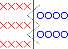
Figure 1: The pitfall of simplicity bias: The solid line is a simple (linear) decision boundary that utilizes only one dimension, while the dashed line is a more complex decision boundary that utilizes two dimensions and maximizes the margin.

Previous studies have empirically shown the robustness of MLM pretrained models. Hao et al. (2019) show that MLM pretraining leads to wider optima and better generalization capability. Hendrycks et al. (2020) and Tu et al. (2020) show that pretrained models are more robust to out-of-distribution data and spurious features. However, it remains unanswered why pretrained models are more robust.

We conjecture that models trained from scratch suffer from the pitfall of simplicity bias Shah et al. (2020) (Figure 1). Shah et al. (2020) and Kalimeris et al. (2019) show that deep networks tend to converge to a simple decision boundary that involves only few features. The networks may not utilize all the features and thus may not maximize the margin, which results in worse robustness. A consequence of this could be that a model may excessively rely on a feature that has spurious association with the label and ignore the other features that are more robust. While Shah et al. (2020) and Kalimeris et al. (2019) investigate networks with continuous input, in Section 2 we demonstrate how spurious features cause problems when the inputs are discrete. Our experimental setting is more related to NLP, where the inputs are discrete.

We start the exploration with the following assumptions: Let the sentence, label pair be $X,Y$.

Assumption 1.

We assume that from $X$, we can extract two features $X_{1}$ and $X_{2}$.

Assumption 2.

$X_{1}$ is a spurious feature that has strong association with $Y$. Specifically, it means that, solely relying on $X_{1}$, one can predict with high accuracy, but cannot be 100% correctly.

Assumption 3.

$X_{2}$ is a robust feature based on which $Y$ can be predicted with 100% accuracy. Namely, there exists a deterministic mapping $f_{X_{2}\to Y}$ that maps $X_{2}$ to $Y$.

The assumptions above are realistic in some NLP tasks. In NLP tasks, the input $X$ is a sequence of tokens. Some tasks satisfy Assumption 1: $X$ can be decomposed into $X_{1}$ and $X_{2}$, where $X_{1}$ is the presence of certain tokens, and $X_{2}$ is the context of the token. As a result, $X_{2}$ has much higher dimensionality than $X_{1}$. Therefore, when Assumption 2 is true, due to the simplicity bias, a deep model is likely to excessively rely on $X_{1}$ and to rely on $X_{2}$ less. However, if Assumption 3 is true, we would desire the model to rely on $X_{2}$, which contains the semantic of the input $X$.

With these assumptions, in Section 3.1 and Section 3.2 we provide a theoretical explanation how MLM pretraining makes a model robust to spurious features. Let $\Pi^{(1)}$ be the conditional probability $P(X_{1}|X_{2})$. We show (1) the relation between the mutual information $I(\Pi^{(1)};Y)\geq I(X_{1};Y)$ and that (2) the convergence rate of learning from $\Pi^{(1)}$ is of the same order as learning from $X_{1}$. That is, when the MLM model can perfectly model the probability $P(X_{1}|X_{2})$ and thus generate perfect $\Pi^{(1)}$, learning from $\Pi^{(1)}$ is as easy as learning from $X_{1}$. As a result, the model will be more likely to avoid the pitfall of simplicity of bias and to rely on $\Pi^{(1)}$. Since $\Pi^{(1)}$ is estimated based on $X_{2}$, higher reliance on $\Pi^{(1)}$ also implies higher reliance on the robust feature $X_{2}$. To relax Assumption 3, we make one step further by considering causal settings in Section 3.3.

The above results partly explain why MLM pretrining is useful for NLP. Denote a sequence of tokens as $X=\langle X_{1},X_{2},\cdots,X_{L}\rangle$. During the MLM pretraining process, each token is masked randomly at certain probability, and the training objective is to predict the masked tokens with maximum likelihood loss. As a result, the model is capable of estimating the conditional probability $P(X_{i}|X\setminus X_{i})$ for all $i=1,2,\cdots,L$. Even though which of the tokens is spurious is unknown, as long as the spurious token has non-zero probability to be masked during pretraining, MLM can estimated its distribution conditioned on the context and thus can reduce the reliance on it.

Finally, we close the gap between our theories and reality. One major gap is that, in reality, we do not use the conditional probability for downstream tasks. Instead, we feed the input $X$ without masking any token and fine-tune the model along with a shallow layer over its output. Regardless of that, we hypothesize that the robustness to spurious tokens brought by MLM pretraining still exists. To prove that, in Section 4 we use the toy example and verify the effect of MLM pretraining when using the common practice for fine-tuning. In Section 5 we validate our theories with two real world NLP tasks.

To sum up, our study leads to new research directions. Firstly, we provide a new explanation of MLM pretraiing’s efficacy. Unlike the previous purely theoretical studies Saunshi et al. (2021); Wei et al. (2021), our assumptions are milder and more realistic. Secondly, we study NLP robustness in a new perspective. Many of the previous studies on robust NLP focus on supervised learning Wang et al. (2021); Utama et al. (2020b; a); Karimi Mahabadi et al. (2020); Chang et al. (2020); He et al. (2019); Sagawa* et al. (2020); Kennedy et al. (2020). However, without self-supervised learning, a model can impossibly extrapolate to out-of-distribution data when the domain shifts. Our work complement previous studies that focus on the bias or robustness of a model generated by the pretraining process Kumar et al. (2020); Hawkins et al. (2020); Vargas & Cotterell (2020); Liu et al. (2020); Gonen & Goldberg (2019); Kurita et al. (2019); Zhao et al. (2019). In this work we investigate the pretraining process itself. Better understanding of pretraining should be important for future research.

2 A Toy Example

With the assumptions, the following toy example and experiment will show that spurious features can cause the difficulty of convergence. Denote the one-hot vector whose $i$th element is $1$ as $e_{i}$. Define $\nu<0.5$ as a flip rate, and let the dimension of the random variables $X_{1}$ and $X_{2}$ be $2$ and $d_{2}$ respectively. Their value $x_{1}\in\{e_{1},e_{2}\}$ and $x_{2}\in\{e_{1},e_{2},\cdots,e_{d_{2}}\}$. Let the middle part of $X_{2}$, the dimensions from $d_{2}/2-\nu d_{2}$ to $d_{2}/2+\nu d_{2}$, be $\dot{X}_{2}$. We consider a joint distribution where $X_{1}=Y$ with probability $1-\nu$, and $X_{1}=1-Y$ when $\dot{X}_{2}\neq 0$. Specifically, we consider the following random process:

$$\begin{split}&X_{2}=e_{i},i\sim\mathrm{Uniform}(1,d_{2})\\ &Y=\begin{cases}-1&\text{if $X_{2}=e_{i}$ for some even $i$}\\ +1&\text{otherwise}\end{cases}\\ &X_{1}=\begin{cases}X_{2}&\text{If $X_{2}=e_{i}$ for some $i$ such that $\lvert i-d_{2}/2\rvert>\nu d_{2}/2$}\\ e_{i},i\sim\mathrm{Uniform}(1,2)&\text{otherwise}\end{cases}\end{split}$$ (1)

Namely $X_{1}$ is flipped with probability 0.5 when the index of the none-zero element of $X_{1}$ is within $d_{2}/2-\lceil d_{2}\nu\rceil$ and $d_{2}/2+\lceil d_{2}\nu\rceil$. In this case, predicting $Y$ solely based on the spurious feature $X_{1}$ can only achieve accuracy $1-\nu$.

We conduct experiments to inspect the effect of the spurious feature $X_{1}$ in this toy model. We train linear networks by drawing batches of i.i.d. $([X_{1};X_{2}],Y)$ pairs from the random process defined in 1. We use Adam optimization with learning rate 0.001 and the cross-entropy loss. In addition to single-layer linear networks, we also try over-parameterized 2-layer and 3-layer linear networks. The hidden size is [10, 32]. Since it is a linear separable problem, we can check whether the learned weight can lead to 100% accuracy in the defined distribution. We check it every 25 iterations. We say a model has converged if it is 100% accurate for 5 consecutive checks. We report the number of the iterations required before it converges for different $\nu$ and $d_{2}$.

Even though it is a linear-separable convex optimization problem, our results in Table 1 show that the spurious feature can impact the number of iterations required to converge. We observe that when $\nu<0.5$, the models tend to be trapped by the spurious feature, sticking at accuracy $1-\nu$ for iterations. When the spurious relation between $X_{1}$ and $Y$ is stronger, i.e. $\nu$ is smaller, the number of iterations required to converge is larger. In addition, the number of iterations is also larger when the $d_{2}$ is larger. An intuitive explanation is that the learning signal from $X_{2}$ is more sparse when $d_{2}$ is larger.

3 A Theoretical Explanation of the Efficacy of MLM Pretraining

3.1 $P(X_{1}|X_{2})$ is More Informative Than $X_{2}$

The toy example above motivate us to consider the information contained in $P(X_{1}|X_{2})$. In the toy example, when predicting $P(Y=0|X)$, if we simply output $P(X_{1}=(1,0)|X_{2})$, then the accuracy of our prediction of $Y$ will be as high as predicting $Y$ solely based on $X_{2}$. It motivates us to inspect the ”reliability” of the estimated $P(X_{1}|X_{2})$ as a feature for the prediction of $Y$ compared to $X_{1}$. Let $\Pi_{1}=P(X_{1}|X_{2})$ be a $|\mathcal{X}_{1}|$-dimensional random variable . In this section we prove that when $P(X_{1}|X_{2})$ is estimated perfectly, $\Pi_{1}$ is at least as informative as $X_{1}$.

Lemma 1.

If it $\Pi_{1}$ perfect, namely $\Pi_{1}=P(\cdot|X_{2})$, then the mutual information $I(X_{1};\Pi_{1})=I(X_{1};X_{2})$.

Proof.

Since $X_{2}$ is discrete, $\Pi_{1}$ is discrete too.

$$H(X_{1}|\Pi_{1})= \sum_{x_{1},\pi_{1}}P(X_{1},\pi_{1})\log P(x_{1}|\pi_{1})$$

$$= \sum_{x_{1},\pi_{1}}\sum_{x_{2}:P(X_{1}|x_{2})=\pi_{1}}P(x_{1},x_{2})\log P(x_{1}|x_{2})=H(X_{1}|X_{2})$$

∎

Compared to previous works Hjelm et al. (2019); Belghazi et al. (2018); Oord et al. (2018) that show some training objectives similar to MLM’s are lower bounds of the mutual information $I(X_{1};X_{2})$, we directly show that the output of the MLM, $\Pi$, maximizes the mutual information, since $I(X_{1};f(X_{2}))\leq I(X_{1};X_{2})$ for any $f$. Moreover, instead of explaining the efficacy of pretraining with the infomax principle Linsker (1988); Bell & Sejnowski (1995), our theories below provide a different perspective.

Theorem 1.

If $\Pi$ is perfect,

$$I(\Pi;Y)\geq I(X_{1};Y)$$ (2)

Proof.

Since $\Pi$ is perfect, by Lemma 1, we have

$$I(X_{1},X_{2})=I(\Pi,X_{2}).$$ (3)

By data processing inequality, the first equality in Equation 3 implies $I(X_{1},X_{2}|\Pi)=0$. By Assumption 3, a deterministic mapping $f_{X_{2}\to Y}$ from $X_{2}$ to $Y$ exists. Applying data processing inequality again, we have

$$\begin{split}I(X_{1},X_{2}|\Pi)\geq I(f_{X_{1}\to Y}(X_{1}),X_{2}|\Pi)=I(Y,X_{2}|\Pi)\geq 0,\end{split}$$ (4)

which implies $I(Y,X_{2}|\Pi)=0$. Accordingly,

$$H(Y|\Pi)=H(Y|X_{2},\Pi)\leq H(Y|X_{2})$$ (5)

∎

Theorem 1 shows that $\Pi$ is a more informative feature than $X_{1}$. However, a model does not necessarily rely more on a more informative feature. We will discuss more in the next section.

		1 layer	2 layers		3 layers
$d1$	$\nu$	w/o	w/o pre	w/ pre	w/o pre	w/ pre
50	0.04	3680 (189.5)	691 (55.8)	614 (169.1)	302 (47.2)	249 (53.7)
50	0.10	2664 (121.2)	530 (30.6)	441 (134.9)	242 (27.6)	180 (37.5)
50	0.25	1420 (96.0)	352 (23.8)	300 (62.0)	179 (13.8)	148 (28.7)
50	0.50	306 (79.8)	141 (40.7)	118 (33.4)	106 (23.1)	89 (24.0)
100	0.04	5466 (170.1)	945 (57.2)	689 (225.3)	431 (51.1)	275 (72.1)
100	0.10	3789 (99.2)	677 (32.2)	478 (142.9)	317 (30.3)	208 (44.3)
100	0.25	1952 (64.9)	428 (13.1)	330 (85.0)	214 (16.2)	169 (32.5)
100	0.50	330 (78.0)	156 (34.0)	133 (41.2)	128 (28.2)	112 (36.1)
500	0.04	11127 (265.9)	1953 (112.5)	857 (442.6)	792 (69.8)	431 (88.4)
500	0.10	7912 (169.2)	1279 (67.5)	657 (234.9)	550 (46.7)	402 (97.0)
500	0.25	4321 (152.3)	772 (35.5)	501 (133.5)	399 (42.3)	391 (66.0)
500	0.50	576 (150.0)	392 (70.2)	407 (81.1)	367 (69.1)	386 (80.0)

Table 1: The number of iterations required to converge. The number is the average of 25 runs with different random seeds, and the number in parentheses is the standard deviation.

3.2 Learning from $\Pi$ is Easy

It is important that learning from $\Pi$ is easy. Because of simplicity bias, a neural network model is likely to rely on the easy-to-learn features due to the simplicity bias Shah et al. (2020); Kalimeris et al. (2019). We conjecture that a model excessively relies on the spurious feature $X_{1}$ when learning from $X_{1}$ is easier than learning from the robust feature $X_{2}$. If learning from $\Pi$ is easy, then the model will rely on $\Pi$ more and thus will rely on $X_{1}$ less. However, features with higher mutual information to $Y$ are not necessarily easy to learn. For instance, models tend to rely on $X_{1}$ instead of $X_{1}$ at the beginning of the training process. MLM can possibly mitigate the issue of spurious features if learning from $\Pi$ is easy.

We show that learning from $\Pi$ is at least as easy as learning from $X_{1}$ by proving the following theorem:

Theorem 2.

Let $\tilde{h}^{(D_{n})}_{X_{1}}$ be the classifier trained with MLE loss using $n$ data pairs $(x^{(1)}_{1},y^{(1)}),(x^{(2)}_{1},y^{(2)}),\cdots(x^{(n)}_{1},y^{(n)})$, and the converged classifier be $\tilde{h}^{*}_{X_{1}}$. Given $P(Y)$, there exists a learning algorithm. It generates $\tilde{h}^{(D_{n})}_{\Pi}$ using $(\pi^{(1)},y^{(1)})$, $(\pi^{(2)},y^{(2)})$, $\cdots$, $(\pi^{(n)},y^{(n)})$ and satisfies the following three properties: (1) $\tilde{h}^{(D_{n})}_{\Pi}$ converges asymptotically no slower than $\tilde{h}^{(D_{n})}_{X_{1}}$ does. (2) Over the distribution of $(X,Y)$, the loss expectation of the converged classifier $\tilde{h}^{*}_{\Pi}$ is no more the expectation of $\tilde{h}^{*}_{X_{1}}$. (3) $\tilde{h}^{*}_{\Pi}$ is a linear model.

Proof.

Proof sketch: The classifier that maximizes the likelihood of $(x^{(1)}_{1},y^{(1)}),(x^{(2)}_{1},y^{(2)}),\cdots(x^{(n)}_{1},y^{(n)})$ can be attained by counting the co-occurrence of $X_{1}$ and $Y$. It converges to

$$\tilde{h}^{*}_{X_{1}}(y|X_{1}=x)=P(y|X_{1}=x).$$ (6)

Based on $\Pi_{1}$, a classifier can be attained by first estimating $P(Y)$ and $P(x_{1}|y)$ for all $x_{1}$ and $y$:

$$\rho_{y}=\frac{\left\lvert\left\{i|y^{(i)}=y\right\}\right\rvert}{n}\quad\rho_{X_{1}|y}^{(n)}=\frac{\sum_{\{i|y^{(i)}=y\}}\pi^{(i)}}{\left\lvert\left\{i|y^{(i)}=y\right\}\right\rvert},$$ (7)

and then we can construct a classifier that converges to

$$\tilde{h}^{*}_{\Pi}(y|\pi)=\sum_{x_{1}}P(y|x_{1})\pi.$$ (8)

For both $\tilde{h}^{*}_{X_{2}}$ and $\tilde{h}^{*}_{\Pi}(y|\pi)$ the $l_{2}$ error converges to $0$ at a rate of $O(\frac{1}{n})$.

Then we show that $\tilde{h}^{*}_{\Pi}(y|\pi)$ is at least as good as $\tilde{h}^{*}_{X_{2}}(y|\pi)$ by showing $D_{KL}[P(Y|X)\;||\;\tilde{h}^{*}_{X_{1}}(Y|X_{1},X_{2},\Pi)]\geq D_{KL}[P(Y|X)\;||\;\tilde{h}^{*}_{\Pi}(Y|X)]$ with convexity:

$$\sum_{x_{1}}P(x_{1}|x_{2})D_{KL}[P(Y|x_{2})\;||\;P(Y|x_{1})]\geq D_{KL}[P(Y|x_{2})\;||\;\sum_{x_{1}}P(Y|x_{1})P(x_{1}|x_{2})].$$ (9)

∎

The remaining question is whether a deep learning model used in common practices can perform at least as well as the algorithm in Theorem 2. Indeed, without any knowledge of deep learning models, it is impossible to theoretically prove that a model will necessarily rely on $\Pi$ instead of $X_{1}$. Therefore, in Section 4 and Section 5 we will empirically validate that our theorems are applicable in the real world scenarios.

3.3 Extending with Causal Models

Before we validate our theories with empiricially, we make a step further by relaxing Assumption 3. We can do so by treating $X_{2}$ as a confounder, and then we can see how MLM pre-training is helpful in the causal and anticausal settings.

Theorem 3.

Even if Assumption 3 is not true, Theorem 1 still holds if $X_{1},X_{2},Y$ follow the causal setting in Figure 3a.

Proof.

By the structure of $X_{1},X_{2},Y$, inequality 4 holds even if the deterministic mapping $f_{X_{2}\to Y}$ does not exist. ∎

Theorem 4.

Assume that the set of vectors $\{P(X_{1}|Y=y)|y\in\mathcal{Y}\}$ is linear independent, and if $X_{1},X_{2},Y$ follow the anticausal setting in Figure 3b, then $I(\Pi,Y)=I(X_{2},Y)$.

Proof.

The assumption is a special case of the one in Lee et al. (2020), so similar techniques can be used: According to the structure of $X_{1},X_{2},Y$, we have

$$P(X_{1}|X_{2})=\sum_{y}P(X_{1}|y)P(y|X_{2}).$$ (10)

Therefore, if $\{P(X_{1}|Y=y)|y\in\mathcal{Y}\}$ is linearly independent, $P(y|X_{2})$ can be recovered from $\Pi=P(X_{1}|X_{2})$. ∎

Note that this theorem is very similar to Theorem 3.3 in Wei et al. (2021). However, the assumptions required in ours are weaker and more realistic, and the implication is very similar. The assumption in Wei et al. (2021) that $X$ is generated from a HMM process with hidden variables $H_{0},H_{1},\cdots$ is a assumption stronger than our assumption that $X_{1},X_{2}$ follows the anticausal setting. The assumption in Wei et al. (2021) that the vectors in $\{P(X_{0}|H_{0}=h)|h\in\mathcal{H}\}$ need to be linearly independent is also less realistic than our independence assumption that requires only the independence in $\{P(X_{1}|Y=y)|y\in\mathcal{Y}\}$, because the number of hidden states $\lvert\mathcal{H}\rvert$ must be very large if $X$ is generated from the HMM model. However, $\lvert\mathcal{Y}\rvert$ tends to be much smaller. For binary classification cases, our assumption holds as long as $P(X_{1})$ is not independent of $P(Y)$. If we further assume that $I(X_{2};Y)=I(X;Y)$, then we reach a similar conclusion that $P(Y|X)$ can be recovered from $\Pi=P(X_{1}|X_{2})$ by applying a linear function.

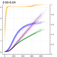
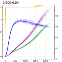
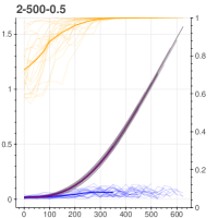
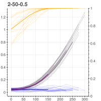
Figure 2: The average weights over the features during training a two-layer model. The upper and the lower rows are the curves of model without and with pretraining respectively. From left to right, $(d_{1},\nu)=(50,0.04),(50,0.5),(500,0.04),(500,0.5)$. Blue, green, purple curves represent the average weights over features in $X_{1}$, $X_{2}$, and $\dot{X}_{2}$ (the middle part of $X_{2}$) respectively. The orange curve represents the accuracy. Note that the scales of the $x$-axis are different in the plots.

3.4 Limitations of Our Theorems

Our theories do not ensure that $\Pi_{1}$ is the most informative feature to learn. Consider tokens in a sentence $X=\langle X_{1},X_{2},\cdots,X_{L}\rangle$ and let $\Pi_{i}$ be the conditional probability $P(X_{i}|X\setminus X_{i})$. A token with spurious association with the label can locate arbitrary position in the sentence, and its location is unknown during pretraining. That is, the pretrained model is able to generate $\Pi_{i}$ for all $i$. Without loss of generality, assume $X_{1}$ is the spurious token. It is possible that there exists some $i$ such that $I(\Pi_{1};Y)<I(\Pi_{i};Y)$, and that $\Pi_{i}$ is predicted relying on $X_{1}$. Concretely, here is an example for the causal setting with three features: $X_{3}$ is independent of $X_{1}$ and $X_{2}$ given $Y$ (Figure 3c). Using the results in Theorem 4, there is a linear mapping that can recover $P(Y|X_{1},X_{2})$ from $\Pi_{3}$. Therefore, it is possible that $I(\Pi_{3};Y)>I(\Pi_{1};Y)$ if $I(X_{1},X_{2};Y)>I(\Pi_{1};Y)$ depending on the distribution of the data. We leave the study of $I(\Pi_{i};Y)$ for future work.

Another limitation is that, in practice, NLP practitioners do not use the conditional probability predicted by the pretrained model. Instead, people stack a simple layer over the pretrained model, and fine-tune the whole model on downstream task. Regardless of this, we conjecture that the outputs generated by feeding the whole sentence without masking also contain the information of $\{\Pi_{i}\}_{i=1}^{n}$ and thus are robust to spurious token-level feature.

4 Toy Example with a Pretrained Model

As the first step to close the gap between our theories and real world, we pretrain the experiment with the toy example. We use the two-layer and three-layer MLP architectures same as in Section 2. Before fitting the model with $Y$, we first pretrain the first layer to predict $X_{1}$ based on $X_{2}$. Specifically, we mask $X_{1}$ when pretraining, so the inputs are $[0,0;X_{2}]$, and the first two dimensions of the outputs are used to compute cross entropy loss. After pretraining, we conjecture that the first two dimensions of the outputs have the equivalent role of $\Pi_{1}$. In order to allow the information from $X_{1}$ to compete with the output of the pretrained part fairly, we manually initialize the weights of the third and fourth dimension of the outputs with $[k,-k,0,\cdots,0]$ and $[-k,k,\cdots,0,0]$ respectively, where $k$ is the average of the absolute value of the weights in the pretrained part. This ensures that the scales of the first four dimensions of the outputs are the same before fine-tuning it with the label $Y$. Finally, we fine-tune the pretrained model with $([X_{1};X_{2}],Y)$ pairs, and report the average number of iterations required to converge for 25 different random seeds.

Table 1 shows that pretraining can always reduce the number of iterations required to converge, when $\nu<0.50$. The effect is more significant when $d_{2}$ equals 100 and 500. It could be because of the higher sparsity of the learning signal.

We further inspect how the product of the weights in the layers change in the process of training. We observe that if the model is not pretrained, the weights over $X_{1}$ grow faster than the weights over $X_{2}$ at the beginning (the first row Figure 2). The model cannot converge to 100% accuracy until weights on $\dot{X}_{2}$, the central $\lceil\nu\times d_{2}\rceil$ dimensions of $X_{2}$, become greater than the weights on $X_{1}$. In addition, after the model converges, weights over $X_{1}$ is still greater than weights over $X_{2}$. On the other hand, if the model is pretrained, weights over $X_{1}$ stop growing after a few steps (the second row in Figure 2). The above observations are aligned with our theorems that pretraining help the model avoid the simplicity bias.

(a) Causal setting

(b) Anticausal setting

(c) A case where $I(\Pi_{3};Y)\geq I(\Pi_{1};Y)$ is possible.

Figure 3: The causal settings of the $(X,Y)$ pairs.

5 Experiments

To further validate our theories, we experiment on real world NLP tasks. We facilitate datasets that have known spurious features. We first pretrain models on the training dataset with different MLM settings. In different settings, the probabilities of masking the spurious tokens are different. Afterward, we fine-tune the model using the target label. We show that the models will be less robust on downstream tasks if spurious tokens are not masked during pretraining, and always masking the spurious token during pretraining improving the robstness. The results validate our theories.

5.1 Dowstream Tasks

Hate Speech Detection

Previous study has shown that hate speech detection datasets tend to have lexical bias Dixon et al. (2018). That is, models rely excessively on the presence or the absence of certain words when predicting the label. Here we follow the formulation of lexical bias in hate speech detection proposed by Zhou et al. (2021). We focus on the effect of non-offensive minority identity (NOI) mentions, such as ”woman”, ”gay”, ”black”. Those mentions are often highly associative with hateful instances. However, it is more desirable that a model does not rely on those mentions. Therefore, we can see the presence of NOI as a spurious feature.

Name Entity Recognition (NER)

Lin et al. (2020) has shown that name entity recognition (NER) models perform worse when the name entities are not seen in the training data. In this case, the content of the name entities can be seen as a spurious feature. Models may learn to memorize the content when fitting the training data, while we may desire the model to recognize name entities according to the context.

5.1.1 Datasets

Hate Speech Detection

We use a portion of the dataset proposed by Zhou et al. (2021). In their original dataset, only a small number of hateful instances contain NOI. Our preliminary experiments show that model without pretraining does not suffer much from the bias of NOI when using the full data. Therefore, we create a dataset of which positive (hateful) samples are all the positive samples in the original dataset that contain NOI, negative samples are negative samples randomly sampled from the original training set. We control the number of negative samples so the ratio of positive and negative samples is the same as the original dataset. We create both the training and the validation splits in this way, and use the original full testing set for evaluation. We also evaluate the models on a NOI subset where all the instances contain NOI.

NER

We use the standard NER dataset Conll-2003 Tjong Kim Sang & De Meulder (2003). To create a testing set with unseen name entities, we replace the name entities in the original validation and testing splits with the entities from WNUT-17 Derczynski et al. (2017). Specifically, we replace the LOC, ORG, PER entities with the corresponding type of entities in WNUT-17, while the MISC entities remain untouched.

5.2 Masking Policies

For each sentence with $n_{s}$ spurious tokens, we experiment with different masking policies: (1) scratch: We do not pretrain the model before fine-tuning. (2) vanilla: During pretraining, we mask each token with 15% probability, which is same as the original setting in Devlin et al. (2019). (3) unmask random: This is similar to vanilla MLM, but we uniformly randomly select $n_{s}$ tokens from the whole sentence and unmask them if they have been masked. (4) unmask spurious: This is similar to vanilla MLM, but we unmask all the spurious tokens. (5) unknown spurious: We replace spurious tokens with a special ”[unk]” token, and we unmask them. Note that this setting can be seen as an oracle setting, since in most applications the spurious features are unknown.

Note that setting (3), (4), (5) have the same expected number of masked tokens. Therefore, it rules out the possibility that the difference between their downstream performance is due to the number of masked tokens. Instead, the difference should be resulted from whether spurious tokens are masked.

Mask Policy	NER		Hate Speech Detection
	Origin	Unseen	All (12893)		NOI (602)
	F1 $\uparrow$	F1 $\uparrow$	Accuracy $\uparrow$	F1 $\uparrow$	Accuracy $\uparrow$	FPR $\downarrow$
scratch	61.5 0.5	38.7 0.6	83.9 1.6	80.3 1.4	74.8 1.5	46.3 7.2
random	74.2 0.4	56.5 1.3	83.1 0.8	78.5 0.8	75.8 0.5	25.1 1.8
unmask random	72.7 0.6	56.5 0.8	83.3 1.1	78.9 1.1	75.8 0.9	25.7 2.3
unmask spurious	72.9 0.5	53.2 0.8	84.1 0.7	79.8 0.6	73.7 1.0	32.5 2.1
unkown spurious	69.8 0.5	56.7 0.8	82.4 1.0	77.8 1.0	77.3 0.6	21.7 2.0

Table 2: The performance on downstream tasks. For the hate speech detection task, we also report false positive detection (FPR) on the NOI subset, which is a set of instances containing non-offensive minority identity mentions, e.g. ”women”, ”black”.

5.3 Implementation Details

For both of the tasks and all the MLM settings, we tokenize the input with the bert-base-uncased tokenizer. We reinitialize all layers except the embedding layer before pretraining, and the embedding layer is frozen through the pretraining process. We train the models until they converge, and choose the one with the lowest MLM loss on the validation set. For the hate speech detection task, we use the implementation provided by Zhou et al. (2021). Except that we use bert-base-uncased instead of roberta-large, we use the other hyper parameters provided in their script. For the NER task, we use the implementation by Hugging Face .

5.4 Result and Discussion

Results in Table 2 validate our theorems. For both of the tasks, unmask random performs better than unmask spurious. Specifically, unmask random has higher F1 on the unseen set of the NER task, and unmask random has low false positive rate (FPR) on the NOI set. Also, unmask random performs similarly to random. This implies that modeling the condition distribution of spurious tokens in the original random masking pretraining can reduce models’ reliance on them. Note that unmask random and unmask spurious have similar in-distribution performance, so the performance difference is not due to better in-distribution generalization suggested by Miller et al. (2021).

We also compare unmask random with the oracle setting unknown spurious. We notice that even though unknown spurious performs as well as random, unknown spurious hurts the performance in the seen set. It indicates that modeling the conditional distribution of spurious tokens has effects beyond simply removing them from the model. On the other hand, unknown spurious performs better in the hate speech detection task. A possible explanation is that NOI mentions contain little useful information for the task.

6 Related Work

Recently, there are efforts attempting to explain the effectiveness of massive language modeling pretraining. Theoretically, Saunshi et al. (2021) explores why auto-regressive language models help solve downstream tasks. However, their explanation is based on the assumption that the downstream tasks are natural tasks, i.e. tasks that can be reformulated as sentence completion tasks. Their explanation also requires the pretrain language model to perform well for any sentence completion tasks, which is not likely to be true in the real world. Wei et al. (2021) analyzes the effect of fine-tuning a pretrained MLM model. Nonetheless, they assume that sentences in natural language are generated by an HMM process, and that the latent state distribution can be recovered from the conditional probability of a token given the context. With a milder assumption, in this work we achieve similar results. Aghajanyan et al. (2020) shows that pretrained models have lower intrinsic dimension, and provides a generalization bound based on Arora et al. (2018). However, why pretrained models have lower intrinsic dimension is still unknown. Empirically, Zhang & Hashimoto (2021) shows that the effectiveness of MLM pretraining cannot be explained by formulating the downstream tasks as sentence completion problems. Sinha et al. (2021) finds evidence supporting the hypothesis that masked language models benefit from modeling high-order word co-occurrence instead of word order. There are also some theories explaining the effective pretraining not specific to MLM Lee et al. (2020); Saunshi et al. (2019); Zhang & Stratos (2021).

7 Implication

Our results provide possible explanations for some common practices that are found effective empirically. First, it could explain why continue pretraining on target dataset is useful. It may be because continue pretraining allows the MLM model to better model the distribution of spurious features in the target dataset. Thus the model can better avoid the simplicity pitfall and converges to a better solution. Second, it provides reasons for more complex masking policies, such as masking a multi-token proper noun at the same time. It may improve the robustness to spurious features that contain more than one token. Third, if MLM can alleviate the simplicity bias and help the model to achieve a greater margin, it may also imply that the model has wider optima. This explains the finding in Hao et al. (2019).

8 Conclusion

In this work, we show an advantage of MLM pretraining, which partly explains its efficacy. We first show the issue of simplicity bias when the input is discrete, and then theoretically and empirically prove that MLM pretraining can alleviate it. Finally, our experiments on real world data also support our theories. Our results shed light on future research on robustness and self-supervised learning.

Appendix A Appendix

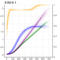
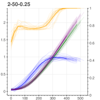
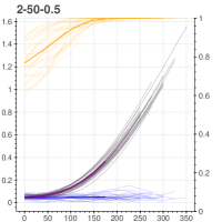
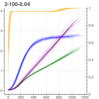
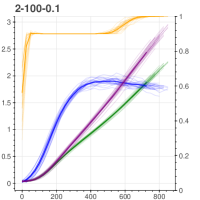
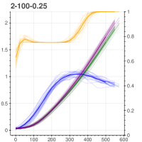
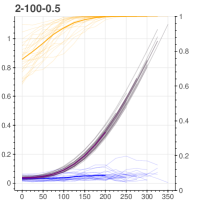
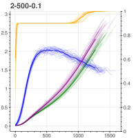
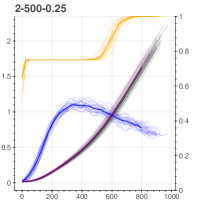
Figure 4: The average weights over the features during training a two-layer model without pretraining. From left to right, $\nu=0.04,0.10,0.25,0.5$. From top to bottom, $d_{1}=50,100,500$. Blue, green, purple curves represent the average weights over features in $X_{1}$, $X_{2}$, and $\dot{X}_{2}$ (the middle part of $X_{2}$) respectively. The orange curve represents the accuracy.

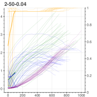
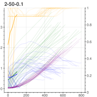
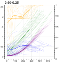
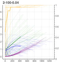
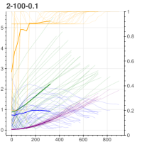
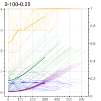
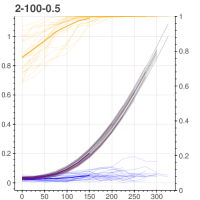
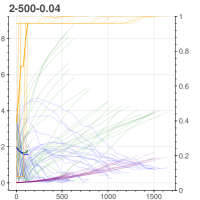
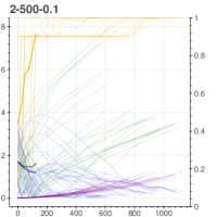
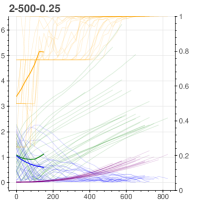
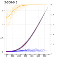
Figure 5: The average weights over the features during training a two-layer model with pretraining. From left to right, $\nu=0.04,0.10,0.25,0.5$. From top to bottom, $d_{1}=50,100,500$. Blue, green, purple curves represent the average weights over features in $X_{1}$, $X_{2}$, and $\dot{X}_{2}$ (the middle part of $X_{2}$) respectively. The orange curve represents the accuracy.

References

- Aghajanyan et al. (2020) Armen Aghajanyan, Luke Zettlemoyer, and Sonal Gupta. Intrinsic dimensionality explains the effectiveness of language model fine-tuning. arXiv preprint arXiv:2012.13255, 2020.
- Arora et al. (2018) Sanjeev Arora, Rong Ge, Behnam Neyshabur, and Yi Zhang. Stronger generalization bounds for deep nets via a compression approach. In International Conference on Machine Learning, pp. 254–263. PMLR, 2018.
- Belghazi et al. (2018) Mohamed Ishmael Belghazi, Aristide Baratin, Sai Rajeshwar, Sherjil Ozair, Yoshua Bengio, Aaron Courville, and Devon Hjelm. Mutual information neural estimation. In Jennifer Dy and Andreas Krause (eds.), Proceedings of the 35th International Conference on Machine Learning, volume 80 of Proceedings of Machine Learning Research, pp. 531–540. PMLR, 10–15 Jul 2018. URL https://proceedings.mlr.press/v80/belghazi18a.html.
- Bell & Sejnowski (1995) Anthony J Bell and Terrence J Sejnowski. An information-maximization approach to blind separation and blind deconvolution. Neural computation, 7(6):1129–1159, 1995.
- Chang et al. (2020) Shiyu Chang, Yang Zhang, Mo Yu, and Tommi Jaakkola. Invariant rationalization. In International Conference on Machine Learning, pp. 1448–1458. PMLR, 2020.
- Derczynski et al. (2017) Leon Derczynski, Eric Nichols, Marieke van Erp, and Nut Limsopatham. Results of the WNUT2017 shared task on novel and emerging entity recognition. In Proceedings of the 3rd Workshop on Noisy User-generated Text, pp. 140–147, Copenhagen, Denmark, September 2017. Association for Computational Linguistics. doi: 10.18653/v1/W17-4418. URL https://www.aclweb.org/anthology/W17-4418.
- Devlin et al. (2019) Jacob Devlin, Ming-Wei Chang, Kenton Lee, and Kristina Toutanova. BERT: Pre-training of deep bidirectional transformers for language understanding. In Proceedings of the 2019 Conference of the North American Chapter of the Association for Computational Linguistics: Human Language Technologies, Volume 1 (Long and Short Papers), pp. 4171–4186, Minneapolis, Minnesota, June 2019. Association for Computational Linguistics. doi: 10.18653/v1/N19-1423. URL https://www.aclweb.org/anthology/N19-1423.
- Dixon et al. (2018) Lucas Dixon, John Li, Jeffrey Sorensen, Nithum Thain, and Lucy Vasserman. Measuring and mitigating unintended bias in text classification. In Proceedings of the 2018 AAAI/ACM Conference on AI, Ethics, and Society, pp. 67–73, 2018.
- Gonen & Goldberg (2019) Hila Gonen and Yoav Goldberg. Lipstick on a pig: Debiasing methods cover up systematic gender biases in word embeddings but do not remove them. In Proceedings of the 2019 Workshop on Widening NLP, pp. 60–63, Florence, Italy, August 2019. Association for Computational Linguistics. URL https://www.aclweb.org/anthology/W19-3621.
- Gururangan et al. (2020) Suchin Gururangan, Ana Marasović, Swabha Swayamdipta, Kyle Lo, Iz Beltagy, Doug Downey, and Noah A. Smith. Don’t stop pretraining: Adapt language models to domains and tasks. In Proceedings of the 58th Annual Meeting of the Association for Computational Linguistics, pp. 8342–8360, Online, July 2020. Association for Computational Linguistics. doi: 10.18653/v1/2020.acl-main.740. URL https://www.aclweb.org/anthology/2020.acl-main.740.
- Hao et al. (2019) Yaru Hao, Li Dong, Furu Wei, and Ke Xu. Visualizing and understanding the effectiveness of BERT. In Proceedings of the 2019 Conference on Empirical Methods in Natural Language Processing and the 9th International Joint Conference on Natural Language Processing (EMNLP-IJCNLP), pp. 4143–4152, Hong Kong, China, November 2019. Association for Computational Linguistics. doi: 10.18653/v1/D19-1424. URL https://www.aclweb.org/anthology/D19-1424.
- Hawkins et al. (2020) Robert Hawkins, Takateru Yamakoshi, Thomas Griffiths, and Adele Goldberg. Investigating representations of verb bias in neural language models. In Proceedings of the 2020 Conference on Empirical Methods in Natural Language Processing (EMNLP), pp. 4653–4663, Online, November 2020. Association for Computational Linguistics. doi: 10.18653/v1/2020.emnlp-main.376. URL https://www.aclweb.org/anthology/2020.emnlp-main.376.
- He et al. (2019) He He, Sheng Zha, and Haohan Wang. Unlearn dataset bias in natural language inference by fitting the residual. In Proceedings of the 2nd Workshop on Deep Learning Approaches for Low-Resource NLP (DeepLo 2019), pp. 132–142, Hong Kong, China, November 2019. Association for Computational Linguistics. doi: 10.18653/v1/D19-6115. URL https://www.aclweb.org/anthology/D19-6115.
- Hendrycks et al. (2020) Dan Hendrycks, Xiaoyuan Liu, Eric Wallace, Adam Dziedzic, Rishabh Krishnan, and Dawn Song. Pretrained transformers improve out-of-distribution robustness. In Proceedings of the 58th Annual Meeting of the Association for Computational Linguistics, pp. 2744–2751, Online, July 2020. Association for Computational Linguistics. doi: 10.18653/v1/2020.acl-main.244. URL https://www.aclweb.org/anthology/2020.acl-main.244.
- Hjelm et al. (2019) R Devon Hjelm, Alex Fedorov, Samuel Lavoie-Marchildon, Karan Grewal, Phil Bachman, Adam Trischler, and Yoshua Bengio. Learning deep representations by mutual information estimation and maximization. In International Conference on Learning Representations, 2019. URL https://openreview.net/forum?id=Bklr3j0cKX.
- Kalimeris et al. (2019) Dimitris Kalimeris, Gal Kaplun, Preetum Nakkiran, Benjamin Edelman, Tristan Yang, Boaz Barak, and Haofeng Zhang. Sgd on neural networks learns functions of increasing complexity. Advances in Neural Information Processing Systems, 32:3496–3506, 2019.
- Karimi Mahabadi et al. (2020) Rabeeh Karimi Mahabadi, Yonatan Belinkov, and James Henderson. End-to-end bias mitigation by modelling biases in corpora. In Proceedings of the 58th Annual Meeting of the Association for Computational Linguistics, pp. 8706–8716, Online, July 2020. Association for Computational Linguistics. doi: 10.18653/v1/2020.acl-main.769. URL https://www.aclweb.org/anthology/2020.acl-main.769.
- Kennedy et al. (2020) Brendan Kennedy, Xisen Jin, Aida Mostafazadeh Davani, Morteza Dehghani, and Xiang Ren. Contextualizing hate speech classifiers with post-hoc explanation. In Proceedings of the 58th Annual Meeting of the Association for Computational Linguistics, pp. 5435–5442, Online, July 2020. Association for Computational Linguistics. doi: 10.18653/v1/2020.acl-main.483. URL https://www.aclweb.org/anthology/2020.acl-main.483.
- Kumar et al. (2020) Vaibhav Kumar, Tenzin Singhay Bhotia, Vaibhav Kumar, and Tanmoy Chakraborty. Nurse is closer to woman than surgeon? mitigating gender-biased proximities in word embeddings. Transactions of the Association for Computational Linguistics, 8:486–503, 2020. doi: 10.1162/tacl˙a˙00327. URL https://www.aclweb.org/anthology/2020.tacl-1.32.
- Kurita et al. (2019) Keita Kurita, Nidhi Vyas, Ayush Pareek, Alan W Black, and Yulia Tsvetkov. Measuring bias in contextualized word representations. In Proceedings of the First Workshop on Gender Bias in Natural Language Processing, pp. 166–172, Florence, Italy, August 2019. Association for Computational Linguistics. doi: 10.18653/v1/W19-3823. URL https://www.aclweb.org/anthology/W19-3823.
- Lee et al. (2020) Jason D Lee, Qi Lei, Nikunj Saunshi, and Jiacheng Zhuo. Predicting what you already know helps: Provable self-supervised learning. arXiv preprint arXiv:2008.01064, 2020.
- Lin et al. (2020) Hongyu Lin, Yaojie Lu, Jialong Tang, Xianpei Han, Le Sun, Zhicheng Wei, and Nicholas Jing Yuan. A rigorous study on named entity recognition: Can fine-tuning pretrained model lead to the promised land? In Proceedings of the 2020 Conference on Empirical Methods in Natural Language Processing (EMNLP), pp. 7291–7300, Online, November 2020. Association for Computational Linguistics. doi: 10.18653/v1/2020.emnlp-main.592. URL https://www.aclweb.org/anthology/2020.emnlp-main.592.
- Linsker (1988) R. Linsker. Self-organization in a perceptual network. Computer, 21(3):105–117, 1988. doi: 10.1109/2.36.
- Liu et al. (2020) Haochen Liu, Wentao Wang, Yiqi Wang, Hui Liu, Zitao Liu, and Jiliang Tang. Mitigating gender bias for neural dialogue generation with adversarial learning. In Proceedings of the 2020 Conference on Empirical Methods in Natural Language Processing (EMNLP), pp. 893–903, Online, November 2020. Association for Computational Linguistics. doi: 10.18653/v1/2020.emnlp-main.64. URL https://www.aclweb.org/anthology/2020.emnlp-main.64.
- Liu et al. (2019) Yinhan Liu, Myle Ott, Naman Goyal, Jingfei Du, Mandar Joshi, Danqi Chen, Omer Levy, Mike Lewis, Luke Zettlemoyer, and Veselin Stoyanov. Roberta: A robustly optimized bert pretraining approach. arXiv preprint arXiv:1907.11692, 2019.
- Miller et al. (2021) John P Miller, Rohan Taori, Aditi Raghunathan, Shiori Sagawa, Pang Wei Koh, Vaishaal Shankar, Percy Liang, Yair Carmon, and Ludwig Schmidt. Accuracy on the line: on the strong correlation between out-of-distribution and in-distribution generalization. In International Conference on Machine Learning, pp. 7721–7735. PMLR, 2021.
- Oord et al. (2018) Aaron van den Oord, Yazhe Li, and Oriol Vinyals. Representation learning with contrastive predictive coding. arXiv preprint arXiv:1807.03748, 2018.
- Sagawa* et al. (2020) Shiori Sagawa*, Pang Wei Koh*, Tatsunori B. Hashimoto, and Percy Liang. Distributionally robust neural networks. In International Conference on Learning Representations, 2020. URL https://openreview.net/forum?id=ryxGuJrFvS.
- Saunshi et al. (2019) Nikunj Saunshi, Orestis Plevrakis, Sanjeev Arora, Mikhail Khodak, and Hrishikesh Khandeparkar. A theoretical analysis of contrastive unsupervised representation learning. In Kamalika Chaudhuri and Ruslan Salakhutdinov (eds.), Proceedings of the 36th International Conference on Machine Learning, volume 97 of Proceedings of Machine Learning Research, pp. 5628–5637. PMLR, 09–15 Jun 2019. URL https://proceedings.mlr.press/v97/saunshi19a.html.
- Saunshi et al. (2021) Nikunj Saunshi, Sadhika Malladi, and Sanjeev Arora. A mathematical exploration of why language models help solve downstream tasks. In International Conference on Learning Representations, 2021. URL https://openreview.net/forum?id=vVjIW3sEc1s.
- Shah et al. (2020) Harshay Shah, Kaustav Tamuly, Aditi Raghunathan, Prateek Jain, and Praneeth Netrapalli. The pitfalls of simplicity bias in neural networks. In NeurIPS, 2020.
- Sinha et al. (2021) Koustuv Sinha, Robin Jia, Dieuwke Hupkes, Joelle Pineau, Adina Williams, and Douwe Kiela. Masked language modeling and the distributional hypothesis: Order word matters pre-training for little. arXiv preprint arXiv:2104.06644, 2021.
- Tjong Kim Sang & De Meulder (2003) Erik F. Tjong Kim Sang and Fien De Meulder. Introduction to the CoNLL-2003 shared task: Language-independent named entity recognition. In Proceedings of the Seventh Conference on Natural Language Learning at HLT-NAACL 2003, pp. 142–147, 2003. URL https://www.aclweb.org/anthology/W03-0419.
- Tu et al. (2020) Lifu Tu, Garima Lalwani, Spandana Gella, and He He. An empirical study on robustness to spurious correlations using pre-trained language models. Transactions of the Association for Computational Linguistics, 8:621–633, 2020. doi: 10.1162/tacl˙a˙00335. URL https://www.aclweb.org/anthology/2020.tacl-1.40.
- Utama et al. (2020a) Prasetya Ajie Utama, Nafise Sadat Moosavi, and Iryna Gurevych. Mind the trade-off: Debiasing NLU models without degrading the in-distribution performance. In Proceedings of the 58th Annual Meeting of the Association for Computational Linguistics, pp. 8717–8729, Online, July 2020a. Association for Computational Linguistics. doi: 10.18653/v1/2020.acl-main.770. URL https://www.aclweb.org/anthology/2020.acl-main.770.
- Utama et al. (2020b) Prasetya Ajie Utama, Nafise Sadat Moosavi, and Iryna Gurevych. Towards debiasing NLU models from unknown biases. In Proceedings of the 2020 Conference on Empirical Methods in Natural Language Processing (EMNLP), pp. 7597–7610, Online, November 2020b. Association for Computational Linguistics. doi: 10.18653/v1/2020.emnlp-main.613. URL https://www.aclweb.org/anthology/2020.emnlp-main.613.
- Vargas & Cotterell (2020) Francisco Vargas and Ryan Cotterell. Exploring the linear subspace hypothesis in gender bias mitigation. In Proceedings of the 2020 Conference on Empirical Methods in Natural Language Processing (EMNLP), pp. 2902–2913, Online, November 2020. Association for Computational Linguistics. doi: 10.18653/v1/2020.emnlp-main.232. URL https://www.aclweb.org/anthology/2020.emnlp-main.232.
- Wang et al. (2021) Liwen Wang, Yuanmeng Yan, Keqing He, Yanan Wu, and Weiran Xu. Dynamically disentangling social bias from task-oriented representations with adversarial attack. In Proceedings of the 2021 Conference of the North American Chapter of the Association for Computational Linguistics: Human Language Technologies, pp. 3740–3750, Online, June 2021. Association for Computational Linguistics. URL https://www.aclweb.org/anthology/2021.naacl-main.293.
- Wei et al. (2021) Colin Wei, Sang Michael Xie, and Tengyu Ma. Why do pretrained language models help in downstream tasks? an analysis of head and prompt tuning. arXiv preprint arXiv:2106.09226, 2021.
- Zhang & Hashimoto (2021) Tianyi Zhang and Tatsunori Hashimoto. On the inductive bias of masked language modeling: From statistical to syntactic dependencies. In Proceedings of the 2021 Conference of the North American Chapter of the Association for Computational Linguistics: Human Language Technologies, pp. 5131–5146, Online, June 2021. Association for Computational Linguistics. URL https://www.aclweb.org/anthology/2021.naacl-main.404.
- Zhang & Stratos (2021) Wenzheng Zhang and Karl Stratos. Understanding hard negatives in noise contrastive estimation. In Proceedings of the 2021 Conference of the North American Chapter of the Association for Computational Linguistics: Human Language Technologies, pp. 1090–1101, Online, June 2021. Association for Computational Linguistics. URL https://www.aclweb.org/anthology/2021.naacl-main.86.
- Zhao et al. (2019) Jieyu Zhao, Tianlu Wang, Mark Yatskar, Ryan Cotterell, Vicente Ordonez, and Kai-Wei Chang. Gender bias in contextualized word embeddings. In Proceedings of the 2019 Conference of the North American Chapter of the Association for Computational Linguistics: Human Language Technologies, Volume 1 (Long and Short Papers), pp. 629–634, Minneapolis, Minnesota, June 2019. Association for Computational Linguistics. doi: 10.18653/v1/N19-1064. URL https://www.aclweb.org/anthology/N19-1064.
- Zhou et al. (2021) Xuhui Zhou, Maarten Sap, Swabha Swayamdipta, Yejin Choi, and Noah Smith. Challenges in automated debiasing for toxic language detection. In Proceedings of the 16th Conference of the European Chapter of the Association for Computational Linguistics: Main Volume, pp. 3143–3155, Online, April 2021. Association for Computational Linguistics. URL https://www.aclweb.org/anthology/2021.eacl-main.274.