Graph Neural Network Guided Local Search for the Traveling Salesperson Problem

Abstract

Solutions to the Traveling Salesperson Problem (TSP) have practical applications to processes in transportation, logistics, and automation, yet must be computed with minimal delay to satisfy the real-time nature of the underlying tasks. However, solving large TSP instances quickly without sacrificing solution quality remains challenging for current approximate algorithms. To close this gap, we present a hybrid data-driven approach for solving the TSP based on Graph Neural Networks (GNNs) and Guided Local Search (GLS). Our model predicts the regret of including each edge of the problem graph in the solution; GLS uses these predictions in conjunction with the original problem graph to find solutions. Our experiments demonstrate that this approach converges to optimal solutions at a faster rate than three recent learning based approaches for the TSP. Notably, we reduce the mean optimality gap on the 100-node problem set from 1.534% to 0.705%, a 2$\times$ improvement. When generalizing from 20-node instances to the 100-node problem set, we reduce the optimality gap from 18.845% to 2.622%, a 7$\times$ improvement.

1 Introduction

Sixty years ago, the route of a delivery truck would have been fixed well before the truck departed the warehouse. Today, thanks to the availability of real-time traffic information, and the option to transmit instructions to the driver to add or remove delivery locations on-the-fly, the route is no longer fixed. Nevertheless, minimizing the length or duration of the route remains an important problem. This is an instance of the Traveling Salesperson Problem (TSP), and one of a growing number of practical applications which require solving combinatorial optimization problems in real time. In these problems, there is often a cost attributed to waiting for an optimal solution or hard deadlines at which decisions must be taken. For example, the driver cannot wait for a new solution to be computed – they may miss their deliveries, or the traffic conditions may change again. There is a need for general, anytime combinatorial optimization algorithms that produce high-quality solutions under restricted computation time. This remains challenging for current approaches, as they are specialized for a specific problem (with specific assumptions and constraints), or fail to produce good solutions quickly.

Contributions   We present a hybrid data-driven approach for approximately solving the Euclidean TSP based on Graph Neural Networks (GNNs) and Guided Local Search (GLS), which we demonstrate converges to optimal solutions more quickly than three recent learning based approaches. We provide the following contributions:

• Our GLS algorithm is guided by the global regret of each edge in the problem graph. This allows the algorithm to differentiate edges that are very costly to include in the solution from ones that are not so costly, whether or not they are part of the optimal solution. Thus, using regret allows us to find high-quality, rather than optimal, solutions very quickly. We are the first to use a measure of global regret, which we define as the cost of enforcing a decision relative to the cost of an optimal solution.

• We make this computationally tractable by approximating regret with a learned representation. Our GNN-based model operates on the line graph of the problem graph, which allows us to build a network without node features, focusing only on edge weight.

• We present experimental results for our approach and several learning based approaches that are aligned with recent guidelines for computational testing of learning based approaches for the TSP. Our experiments emphasize the trade-off between solution quality and time.

• We reduce the mean optimality gap on the 50-node problem set from 0.268% to 0.009%, a 30$\times$ times improvement, and on the 100-node problem set from 1.534% to 0.705%, a 2$\times$ improvement. When generalizing from 20-node instances to the 100-node problem set, we reduce the mean optimality gap from 18.845% to 2.622%, a 7$\times$ improvement.

2 Related Work

The Operations Research (OR) community is responsible for the majority of research in algorithms for solving combinatorial optimization problems. Concorde (Applegate et al., 2006) is widely regarded as the best exact TSP solver. As an exact solver, it can guarantee the level of optimality of the solutions it finds. It uses cutting plane algorithms (Dantzig et al., 1954; Padberg & Rinaldi, 1990; Applegate et al., 2003) and branch-and-cut methods to iteratively prune away parts of search space that will not contain an optimal solution. LKH-3 (Helsgaun, 2017), and its predecessor, LKH-2 (Helsgaun, 2009), are approximate TSP and Capacitated Vehicle Routing Problem (CVRP) solvers based on the $\kappa$-opt heuristic (Lin & Kernighan, 1973). While these solvers do not provide any guarantees, experimentation has demonstrated that they are extremely effective. Concorde, LKH-2 and LKH-3 are highly specialized and efficient solvers which can solve challenging TSPs in seconds.

However, practical real-time routing problems often impose constraints on top of the basic TSP or CVRP problem definitions. Highly-specialized solvers are difficult to adapt to these new constraints. Thus, there is a need for general algorithmic frameworks that can produce high-quality solutions with minimal computation time. To address this, Arnold & Sörensen (2019a) introduce KGLS, a GLS algorithm for the CVRP that is guided by three engineered features. They demonstrate that their algorithm can find solutions almost as good as those found by state-of-the-art metaheuristics in a fraction of the time. Our work also aims to address this gap.

Machine learning offers a way to construct flexible, yet effective combinatorial optimization algorithms. This area of research has existed for more than three decades (Smith, 1999), yet new neural architectures, especially GNNs, have driven a surge of activity in this area. As noted by Bengio et al. (2021); Cappart et al. (2021), classical combinatorial optimization approaches solve each problem instance in isolation, overlooking the fact that in practice, problems and their solutions stem from related data distributions. Machine learning offers a way to exploit this observation. We classify learning based approaches for solving the TSP into the three categories identified by Bengio et al. (2021); our approach belongs to the second category, described below.

ML alone provides a solution.   These approaches use a machine learning model to output solutions directly from the problem definition. Vinyals et al. (2015) propose PtrNet, a sequence-to-sequence model based on LSTMs, which iteratively constructs a solution by outputting the permutation of the input nodes. They train their model using expert solutions from Concorde. They use beam search (Reddy, 1977) to produce better solutions than those sampled from their model directly. Bello et al. (2016) present a method of training PtrNet without supervision using policy gradients. Their “active search” method resembles early neural network-based approaches to combinatorial optimization, in which a model was trained online to solve a particular problem instance (Smith, 1999). This method effectively solves each problem in isolation, thus it does not leverage expertise extracted from distribution of training problem instances. Kool et al. (2018) take a similar approach to Bello et al. (2016) but use a Transformer architecture (Vaswani et al., 2017) rather than an LSTM. Their model can also be seen as a Graph Attention Network (GAT) (Veličković et al., 2017) applied to a complete graph. Kwon et al. (2021) also take a similar approach but leverage the symmetry of many combinatorial optimization problems to improve performance.

Joshi et al. (2019) train a model to produce a heatmap of which edges in the TSP graph are likely to be part of the optimal solution, and reconstruct valid tours using beam search. Similar to Vinyals et al. (2015), they train their model using expert solutions from Concorde. Kool et al. (2021) extend the work of Joshi et al. (2019) to VRPs, and use a dynamic programming method to construct tours. Also in this category, Fu et al. (2021) train a model to output a heatmap for small TSP instances to and sample small sub-graphs from large instances to construct heatmaps for large instances. They train their approach using reinforcement learning, and use Monte Carlo tree search (MCTS) to construct valid tours.

ML provides information to an OR algorithm.   Machine learning may not be suitable to solve a combinatorial optimization problem alone. Instead, it can provide information to augment a combinatorial optimization algorithm. Deudon et al. (2018) use a model based on the Transformer architecture to construct solutions iteratively and train it using policy gradients (they take a similar approach to Kool et al., 2018). They apply a 2-opt local search heuristic to solutions sampled from their model. In contrast to prior work, we are the first to use a machine learning model to approximate regret. Furthermore, many previous works that produce predictions on edges (Joshi et al., 2019; Kool et al., 2021; Fu et al., 2021) construct tours using heuristics, whereas to our knowledge, we are the first to use predictions to inform a metaheuristic (GLS).

ML makes decisions within an OR algorithm.   Finally, a machine learning model can be embedded inside a combinatorial optimisation algorithm. In this paradigm, a master algorithm controls the high-level procedure while repeatedly calling a machine learning model to make lower level decisions. Dai et al. (2017) present a model that uses a GNN to learn an embedding of the current partial solution and a DQN (Mnih et al., 2015) to iteratively select nodes to insert using a cheapest insertion heuristic. They also use an “active search” method when solving the TSP. Wu et al. (2020) and da Costa et al. (2020) present policy gradient algorithms to learn policies to apply 2-opt operations to existing feasible solutions. Wu et al. (2020) use a Transformer architecture. da Costa et al. (2020) use a combination of GCN and RNN modules, and acheive better results. These approaches can either be seen as end-to-end learning approaches belonging to the first category, or as local search procedures where an ML model decides where to apply an operator.

3 Preliminaries

Traveling Salesperson Problem   We focus on the Euclidean TSP, although our approach can be applied to other routing problems, such as the CVRP. A problem with $n$ cities, typically denoted TSP$n$, is represented as a complete, undirected, weighted graph $G=(V,E)$ with $n$ nodes. The edges $E$ represent connections between cities and are weighted by the Euclidean distance between the adjacent nodes. A solution, or tour, is a Hamiltonian cycle: a closed path through the graph that visits every node exactly once. An optimal solution is a cycle of minimum weight.

Regret   Regret measures the future cost of an action that also yields an immediate reward, and is typically used to make greedy combinatorial optimization algorithms less myopic. Generally, regret is computed over a fixed horizon. For example, Potvin & Rousseau (1993) evaluate the cost of inserting a node in the best versus second-best position when constructing a CVRP solution. Hassin & Keinan (2008) solve the TSP using regret, allowing a greedy construction heuristic to remove the most recently inserted node. It is not computationally feasible to calculate regret over a global horizon, for example, for all possible insertion sequences. However, if it were possible, a greedy algorithm could compute an optimal solution by selecting the lowest regret decision at each step.

Local Search   Local Search (LS) is a general improvement heuristic. Starting from an initial solution, local search iteratively moves to neighboring solutions that are lower cost than the current solution according to the objective function $g(s)$. Neighboring solutions are solutions that are reachable from a given solution by applying a certain function, or operator. The set of all solutions reachable from another solution by applying an operator define the neighborhood of that operator. The algorithm terminates when all neighboring solutions are inferior to the current solution, meaning the search has reached a local optimum.

Guided Local Search   Guided Local Search (GLS) is a metaheuristic that sits on top of LS and allows it to escape local optima (Voudouris & Tsang, 1996). To apply GLS, the designer must define some aspects of a solution. When trapped in a local optimum, the algorithm penalizes certain aspects of the current solution which are considered to be unfavorable. The underlying LS procedure searches using an objective function that is augmented by these penalties, thus it is incentivized to remove heavily penalized aspects from the solution. The augmented objective function $h(s)$ is

$$h(s)=g(s)+\lambda\sum_{i=0}^{M}p_{i}I_{i}(s),$$ (1)

where $s$ is a solution, $g(s)$ is the objective function, $\lambda$ is a scaling parameter, $i$ indexes the aspects, $M$ is the number of aspects, $p_{i}$ is the current number of penalties assigned to aspect $i$, and $I_{i}$ is an indication of whether $s$ exhibits aspect $i$, i.e.

$$I_{i}(s)=\begin{cases}1&\text{if }s\text{ exhibits aspect }i,\\ 0&\text{otherwise.}\end{cases}$$ (2)

For the TSP, aspects of the solution are often defined as the edges in the problem graph. Therefore, $I_{i}(s)$ indicates if an edge is in the solution $s$. Upon reaching a local optimum, which aspects are penalized is determined by a utility function. The utility of penalising aspect $i$, $\text{util}_{i}$, is defined as

$$\text{util}_{i}(s_{*})=I_{i}(s_{*})\frac{c_{i}}{1+p_{i}},$$ (3)

where $s_{*}$ is the solution at a local optimum, $I_{i}(s_{*})$ indicates if the solution exhibits aspect $i$, and $c_{i}$ is the cost of the aspect $i$. The cost of an aspect measures how unfavorable it is. The higher the cost, the greater the utility of penalizing that aspect. In the context of the TSP, the cost can be the weight of the edge (Voudouris & Tsang, 1999), or a combination of various features (Arnold & Sörensen, 2019a). Conversely, the more penalties assigned to that aspect, the lower the utility of penalising it again. The aspects with the maximum utility are always penalized, which means increasing $p_{i}$ by one. This penalization mechanism distributes the search effort in the search space, favoring areas where a promise is shown (Voudouris & Tsang, 1996).

We use a variation of the classical GLS algorithm (see Voudouris & Tsang, 1999) that applies alternating optimisation and perturbation phases (see Arnold & Sörensen, 2019a). During an optimization phase, the local search procedure is guided by the original objective function $g$. During a perturbation phase, it is guided by the augmented objection function $h$. After an edge is penalized, the local search is applied only on the penalized edge. That is, only operations that would remove the penalized edge are considered. This differs from the local search during the optimization phase, which considers all solutions in the neighborhood of the given operator. The perturbation phase continues until $K$ operations (operations that improve the solution according to the augmented objective function $h$) have been applied to the current solution. These operations perturb the solution enough for the local search to escape a local minimum. The alternating phases continue until the stopping condition is met.

4 Method

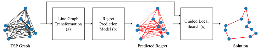
Figure 1: From a TSP formulated as a graph, we take the line graph (a) and input it into our regret approximation model (b), which predicts the regret of including each edge in the solution. GLS (c) uses these predictions in conjunction with the original problem graph to quickly find a high-quality solution.

Our hybrid method, shown in Figure 1, combines a machine learning model and a metaheuristic. Our GNN-based model learns an approximation of the global regret of including each edge of the problem graph in the solution. The metaheuristic, GLS, uses this learned regret conjunction with the original problem graph to quickly find high-quality solutions. The learned regret allows the algorithm to differentiate between edges which are costly to include in the solution and ones that are not so costly, thus improving its ability to steer the underlying local search procedure out of local minima and towards promising areas of the solution space.

4.1 Global Regret

We define global regret as the cost of requiring a certain decision to be part of the solution relative to the cost of a globally optimal solution. Unlike previous heuristics using regret, which calculate the cost of a decision relative to some fixed number of alternatives (for example, the next best, or two next best options), our regret is measured relative to a global optimal solution. Decisions that are part of an optimal solution have zero regret, and all other decisions have positive regret. Mathematically,

$$r_{i}=\frac{g(s_{i}^{*})}{g(s^{*})}-1,$$ (4)

where $r_{i}$ is the regret of decision $i$, $g$ is the objective function, $s_{i}^{*}$ is an optimal solution with $i$ fixed, and $s^{*}$ a globally optimal solution. With perfect information, a greedy algorithm could construct an optimal solution by sequentially selecting the lowest-regret decisions.

In the TSP, decisions correspond to which edges are included in the solution, thus regret is defined as the cost of requiring that a certain edge be part of the solution. We posit that using regret is preferable to directly classifying which edges are part of the optimal solution (which is the approach taken by Joshi et al., 2019). Where classification can produce a probability that the edge is part of optimal solution, regret can differentiate between edges that are very costly to have as part of the solution and ones that are not so costly, whether or not they are part of the optimal solution. Thus, using regret furthers our goal of finding high-quality, rather than optimal, solutions with minimal computation time.

4.2 Regret Approximation Model

Calculating the global regret of an edge in the TSP graph requires solving the TSP itself, which is computationally intractable. Instead, we aim to learn a function $\hat{r}_{ij}$ that approximates the regret of an edge $r_{ij}$. We use GNNs to achieve this, as they are universal function approximators that operate on graph-structured data.

Input transformation   Typically, GNNs aggregate messages and store states on the nodes of a graph (Gilmer et al., 2017). Instead, we input the line graph of the original problem graph into our model. The line graph $L(G)$ of an undirected graph $G$ is a graph such that there exists a node in $L(G)$ for every edge in $G$, and that for every two edges in $G$ that share a node, there exists an edge between their corresponding nodes $L(G)$. Figure 2 illustrates this transformation for a simple graph. The result is that our model aggregates messages and stores states on the edges of the problem graph (the nodes of the line graph). Primarily, this allows us to build models with no node features, which is advantageous as the edge weights, not the specific node locations, are relevant when solving the TSP. For a complete, undirected graph $G$ with $n$ nodes, there are $n(n-1)/2$ nodes and $n(n-1)(n-2)$ edges in $L(G)$. Thus, although $G$ is complete, $L(G)$ can be very sparse.

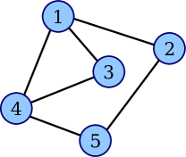
(a) $G$

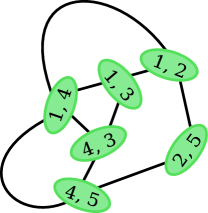
(b) $L(G)$

Figure 2: An example of a graph and the corresponding line graph. The edges in $G$ are the nodes in $L(G)$, and vice-versa.

Model architecture   Our model consists of an embedding layer, several GNN layers, and an output layer. The embedding layer is an edge-wise fully connected layer that computes $d_{h}$-dimensional edge embeddings from $d_{x}$-dimensional edge features. Node features, if used, are concatenated onto the feature set of the adjacent edges. The forward pass of the embedding layer is written as

$$\mathbf{h}_{ij}^{0}=\mathbf{Wx}_{ij}+\mathbf{b},$$ (5)

where $\mathbf{h}_{ij}^{0}$ is the initial embedding of edge $ij$, $\mathbf{W}$ is a learnable weight matrix, $\mathbf{x}_{ij}$ are the input features of edge $ij$ (including any node features), and $\mathbf{b}$ is a set of learnable biases. We use $d_{x}=1$ and $d_{h}=128$. The edge embeddings are updated using $T$ message passing layers. Inspired by the encoder layer of Kool et al. (2018), each layer consists of multiple sublayers. The forward pass is given by

$$\dot{\mathbf{h}}_{ij}^{t+1} =f_{\text{BN}}^{t}(\mathbf{h}_{ij}^{t}+f_{\text{MHA}}^{t}(\mathbf{h}_{ij}^{t},L(G))),$$ (6)

$$\mathbf{h}_{ij}^{t+1} =f_{\text{BN}}^{t}(\dot{\mathbf{h}}_{ij}^{t+1}+f_{\text{FF}}^{t}(\dot{\mathbf{h}}_{ij}^{t+1})),$$ (7)

where $f_{\text{MHA}}$ is a multi-headed GAT layer (Veličković et al., 2017), $f_{\text{FF}}$ is a feedforward layer, $f_{\text{BN}}$ is batch normalisation (Ioffe & Szegedy, 2015), and $\dot{\mathbf{h}}_{u}^{t+1}$ is a hidden state. The layers do not share parameters. The GAT layer uses $M=8$ heads and dimensionality $d_{h}/{M}=16$, and the FF layer uses one hidden sublayer with dimensionality 512 and ReLU activation. Finally, the output layer is a single edge-wise fully connected layer that computes a one-dimensional output from the $d_{h}$-dimensional node embeddings computed by the final message passing layer. This is written as

$$\hat{r}_{ij}=\mathbf{Wh}_{ij}^{T}+\mathbf{b},$$ (8)

where $\hat{r}_{ij}$ is the output for edge $ij$ and $\mathbf{h}_{ij}^{T}$ is the final embedding of that edge.

4.3 Regret-Guided Local Search

We adapt GLS to use regret to solve the TSP, including how the initial solution is built, the local search procedure, and the perturbation strategy. Our GLS uses alternating optimization and perturbation phases. During an optimization phase, the local search procedure greedily accepts changes to the solution until it reaches a local minimum. During a perturbation phase, the algorithm penalizes and attempts to remove edges in the current solution with high regret, thus allowing it to escape local minima while simultaneously guiding it towards promising areas of the solution space, i.e., those with low regret. Effectively, the regret predictions produced by our model allow our GLS algorithm to undo costly decisions made during the greedy optimization phase.

Initial solution   We use a greedy nearest neighbor algorithm to construct an initial solution. Beginning from the origin node we iteratively select the lowest-regret edge leading to an unvisited node, until all nodes have been visited.

Local Search neighborhoods   Our LS procedure uses two solution operators for the TSP, relocate and 2-opt. It alternates between using either operator, and uses a “best improvement” strategy, meaning that it exhaustively searches the neighborhood corresponding with the current operator and accepts the solution that improves the objective function the most before continuing with the other operator. The algorithm terminates when no improvement can be found in either neighborhood. The relocate operator simply changes the position of a single node in the tour. The 2-opt operator selects two nodes in the tour to swap. This divides the tour into three segments: an initial segment, an intermediate segment, and a final segment. The tour is reassembled beginning with the initial segment, the intermediate segment in reverse order, and the final segment. It is a special case of the $\kappa$-opt operator (Lin & Kernighan, 1973), although it was introduced earlier (Croes, 1958).

Perturbation strategy   We define the cost of an edge as the predicted regret $\hat{r}_{ij}$ of that edge. The utility of penalizing edge $ij$, $\text{util}_{ij}$, is therefore defined as

$$\text{util}_{ij}(s_{*})=I_{ij}(s_{*})\frac{\hat{r}_{ij}}{1+p_{ij}},$$ (9)

where we remind the reader that $s_{*}$ is the solution at a local optimum, $I_{ij}(s_{*})$ indicates if the solution contains edge $ij$, and $p_{ij}$ is the number of penalties assigned to that edge. The edges of maximum utility are penalized. Afterward, the local search is applied only on the penalized edge. That is, only operations that would remove the penalized edge are considered.

5 Experiments

We train our model using supervised learning. It uses a single input feature, edge weight (i.e. the Euclidean distance between adjacent nodes), to predict the regret of the edges in the problem graph. Further details of our implementation are found in Appendix A. While further input features could be considered, they come at a computational cost, as seen in Table 4. In Appendix D, we compare 11 input features, and demonstrate that edge weight is the most important feature when predicting the regret of an edge.

Evaluation   We evaluate the trade-off between solution quality and computation time when solving randomly generated TSPs as well as TSPLIB instances. Where available, we use publicly available implementations and pre-trained models. There is no publicly available implementation of Arnold & Sörensen (2019a), so we use the GLS implementation described in section 4.3 with the guides described in their paper.

We compare our approach to the following methods, the first six of which are non-learning based, and the other three are learning based:

1. Nearest Neighbour

2. Farthest Insertion

3. Local Search (as described in section 4.3)

4. Concorde (Applegate et al., 2006)

5. LKH-3 (Helsgaun, 2017)

6. kglstitle (Arnold & Sörensen, 2019a)

7. attentionlearntosolvetitle (Kool et al., 2018)

8. gcntsptitle (Joshi et al., 2019)

9. learn2opttitle (da Costa et al., 2020)

Following comp_guidelinestitle (Accorsi et al., 2021), we conduct two types of experiments. 1) we leave both computation time and solution quality unfixed. We measure the mean optimality gap and computation time per instance across the entire problem set. We use implementations as-described. 2) we fix computation time and measure the solution quality, in terms of mean optimality gap and the number of instances solved optimally. This allows for a direct comparison of approaches that was impossible in the first experiments and previous works. Where possible, we modified implementations to run continuously until the computation time limit is reached. We allow up to 10 seconds to solve each problem, including the time required to calculate input features, evaluate a model, or to construct an initial solution.

We evaluate the problem sets one instance at a time, which allows us to accurately measure computation time per instance. We allow parallelism in the GPU to sample multiple solutions to a single problem at once, where implementations are configured to do so. We use a common, single CPU and single GPU setup for all experiments. More details on the experimental setup and the hyperparameters of different approaches are given in Appendix A.

We conduct both types of experiments on three problem sets, TSP20, TSP50, and TSP100, consisting of one thousand 20, 50, and 100-node 2D Euclidean TSP instances, respectively. We generate the instances by uniform-randomly sampling node locations in the unit square $[0,1]^{2}$, which is in line with the methods used by Kool et al. (2018); Joshi et al. (2019); da Costa et al. (2020). In the second type of experiment (fixed computation time), we focus on the learning based approaches and keep Concorde as a benchmark. Furthermore, we evaluate the generalization performance of the learning based approaches from smaller to larger problem sets, and from the randomly generated instances to TSPLIB instances, which are meant to represent real-world problems.

Results   The performance of each approach when computation time and solution quality are unfixed is shown in Table 1. Approaches that are not dominated by others (i.e. they produce higher-quality solutions or are faster) are bolded. These values form a Pareto front for the trade-off between solution quality and computation time. Non-learning and learning approaches are considered separately. Our approach always lies on the Pareto front. These results are visualized in Figure 3 in Section B.1. The results presented for Joshi et al. (2019) differ from the results presented by the authors, due to an implementation error we found in their code (see Appendix A for the correction).

Problem	Method	Computation time (s)	Optimality gap (%)
TSP20	Nearest Neighbor	0.000±0.000	17.448±10.209
	Farthest Insertion	0.005±0.000	2.242±2.536
	Local Search	0.007±0.003	1.824±3.254
	Arnold et al.	10.009±0.008	0.000±0.000
	Concorde	0.119±0.083	0.000±0.000
	LKH-3	0.020±0.019	0.000±0.000
	Kool et al.	0.038±0.005	0.069±0.255
	Joshi et al.	1.344±0.106	2.031±2.928
	O. da Costa et al.	21.120±0.352	0.001±0.025
	Ours	10.010±0.008	0.000±0.000
	Kwon et al.*	–	0.00
	Fu et al.*	–	0.000
TSP50	Nearest Neighbor	0.002±0.000	23.230±7.968
	Farthest Insertion	0.065±0.001	7.263±3.072
	Local Search	0.101±0.031	3.357±2.603
	Arnold et al.	10.035±0.039	0.040±0.180
	Concorde	0.258±0.197	0.000±0.000
	LKH-3	0.069±0.030	0.000±0.012
	Kool et al.	0.124±0.006	0.494±0.655
	Joshi et al.	3.080±0.182	0.884±1.700
	O. da Costa et al.	24.338±0.523	0.136±0.314
	Ours	10.037±0.039	0.009±0.069
	Kwon et al.*	–	0.03
	Fu et al.*	–	0.0145
TSP100	Nearest Neighbor	0.010±0.000	25.104±6.909
	Farthest Insertion	0.444±0.010	12.456±2.944
	Local Search	0.727±0.165	4.169±2.047
	Arnold et al.	10.128±0.194	1.757±1.240
	Concorde	0.573±0.771	0.000±0.000
	LKH-3	0.118±0.022	0.011±0.058
	Kool et al.	0.356±0.007	2.368±1.185
	Joshi et al.	6.127±0.081	1.880±4.097
	O. da Costa et al.	30.656±0.734	0.773±0.717
	Ours	10.108±0.175	0.698±0.801
	Kwon et al.*	–	0.14
	Fu et al.*	–	0.037

Table 1: Solution quality and computation time for various approaches. Means and standard deviations are reported, calculated across the entire problem set. Pareto optimal values (i.e. faster or better solutions) are bolded. Some results (*) are taken directly from papers that do not report computation time per instance, and thus cannot be compared.

To better evaluate this trade-off, the second experiment fixes computation time and measures the solution quality as it evolves over time. Figure 4 in Section B.2 visualizes the performance as a function of time, which provides a rich understanding of the trade-off made by each approach. Table 2 shows the performance of the learning based approaches after 10 seconds of computation time per instance. Our approach finds better solutions on average than the other approaches for all problem sets. Notably, we reduce the mean optimality gap on the 50-node problem set from 0.268% to 0.009%, a 30$\times$ times improvement, and on the 100-node problem set from 1.534% to 0.705%, a 2$\times$ improvement. Joshi et al. (2019) finds more optimal solutions to the TSP100 problem set, but has worse average performance than our approach. Our approach finds more optimal solutions to the TSP20 and TSP50 problem sets than the other approaches.

Problem	Method	Optimality gap (%)	Optimal solutions (%)
TSP20	Concorde	0.000±0.000	100.0000
	Kool et al.	0.069±0.255	84.6000
	Joshi et al.	1.000±12.492	97.4000
	O. da Costa et al.	0.002±0.027	99.0000
	Ours	0.000±0.000	100.0000
TSP50	Concorde	0.000±0.000	100.0000
	Kool et al.	0.494±0.655	29.5000
	Joshi et al.	1.206±18.066	86.3000
	O. da Costa et al.	0.268±0.492	48.7000
	Ours	0.009±0.069	96.2000
TSP100	Concorde	0.000±0.000	100.0000
	Kool et al.	1.958±1.064	0.3000
	Joshi et al.	1.559±4.071	51.6000
	O. da Costa et al.	1.534±1.098	1.4000
	Ours	0.705±0.807	20.5000

Table 2: Solution quality measured after after 10 seconds of computation time per instance. The mean optimality gap and standard deviation, as well as the percentage of optimally solved problems are reported. Our approach converges to better solutions at a faster rate than the other approaches.

We evaluate the performance of our approach and other learning based approaches when generalizing from smaller instances to larger ones, and from randomly generated instances to TSPLIB instances, which are meant to represent real-world instances. These results are summarized in Section C.1 and Section C.2 respectively. Our approach generalizes well. Notably, when generalizing from 20-node instances to the 100-node problem set, we reduce the mean optimality gap from 18.845% to 2.622%, a 7$\times$ improvement.

6 Discussion

Our approach generalizes to larger problems and to real-world problems well, which may be due to the unique input transformation we apply to the problem graph. We input the line graph $L(G)$ of the problem graph $G$, which allows the model to aggregate messages and store states on edges rather than nodes. This allows us to build models without node features, which is advantageous as the edge weights, not the specific node positions, are relevant when solving the TSP. Including the node positions as features, as done by Kool et al. (2018); Joshi et al. (2019); da Costa et al. (2020) may hinder the learned policy’s ability to generalize. Deudon et al. (2018) apply PCA on the node positions before inputting them into their model so they are rotation invariant, yet they do not report generalization performance. For a Euclidean TSP problem graph with $n$ nodes, $L(G)$ has $n(n-1)/2$ nodes, meaning that although $G$ is complete, $L(G)$ can be very sparse, which may help learning (Cappart et al., 2021). However, the model consumes more GPU memory than models using the problem graph $G$.

Many approaches that learn construction heuristics (for example Kool et al., 2018) treat the tour as a permutation of the input nodes. By considering the solution as a sequence, these approaches miss out on its symmetry: a TSP solution is invariant to the origin city. Outputting the correct sequence becomes increasingly difficult as the number of cities increases. This has recently been addressed by Kwon et al. (2021), who leverage the symmetry of the TSP in their approach. Our model learns the regret of including a given edge in the solution based on its features and those of its neighbors, which implicitly assumes the symmetry of a TSP solution.

We argue that our hybrid architecture is more general than others, as our global regret is defined for most routing problems. When applying our method to a new routing problem, the designer need only plug-and-play a local search procedure that is appropriate for the problem. In contrast, methods which learn heuristics cannot always be transferred to other problems. For example, 2-opt cannot be used on routing problems that include pickup and drop-off constraints (Pacheco et al., 2021). A drawback of our approach is that it relies on supervised learning. In future work, our regret approximation model could be trained end-to-end.

7 Conclusion

We present a hybrid data-driven approach for solving the TSP based on Graph Neural Networks (GNNs) and Guided Local Search (GLS). To inform GLS, we use a GNN-based model to compute fast, generalizable approximations of the global regret of each edge. Our model operates on the line graph of the TSP graph, which allows us to build a network that uses edge weight as the only input feature. This approach allows our algorithm to escape local minima and find high-quality solutions with minimal computation time. Finally, we present experimental results for our approach and several recent learning based approaches that emphasize the trade-off between solution quality and computation time. We demonstrate that our approach converges to optimal solutions at a faster rate than the evaluated learning based approaches.

Appendix A Implementation details

We conduct all computational experiments on virtual machines using a single core of an Intel Xeon E5-2650 v4 processor, 24 GB of RAM, and a single Tesla P100 GPU with 16 GB of VRAM. We evaluate the various approaches one-at-a-time, to ensure they do not compete for computational resources. When evaluating the various approaches, we record actual tours and use a common method of calculating tour cost and optimality gap, as we found that small discrepancies in cost calculations between implementations led to skewed results. We recommend this approach when comparing different approaches for solving the TSP. Based on approximately 200,000 TSP solutions, we determined that an absolute threshold of $10^{-7}$ on the value of the objective function is sufficient to separate optimal and sub-optimal solutions.

We train our model on sets of one hundred thousand 20, 50, and 100-node 2D Euclidean TSP instances. We generate all instances by uniform-randomly sampling node locations in the unit square $[0,1]^{2}$. We calculate the target output, the regret of including each edge in the solution, according to eq. 4. We use Concorde to find an optimal solution and LKH-3 with 100 trials and 10 runs to solve find an optimal solution with a given edge fixed. We empirically validate that this configuration for LKH-3 is sufficient to find optimal solutions for problems with 100 nodes or less. We scale the input features and target outputs to a range of $[0,1]$.

We train our model by minimizing the $l^{2}$ loss to the target output using the Adam optimizer (Kingma & Ba, 2014) and an exponentially decaying learning rate $\gamma=10^{-3}\times(0.99)^{e}$, where $e$ is the epoch. We train the model for 100 epochs with early stopping. We use a training batch size $B=32$ for the 20 and 50-node training sets, and a training batch size of $B=15$ for the 100-node training set due to limited GPU memory. Our model uses $T=3$ message passing layers and our GLS algorithm uses $K=20$ perturbation moves. Our approach is implemented using Python 3.8.11, PyTorch 1.9.0 (Paszke et al., 2019), DGL 0.7.1 (Wang et al., 2019), and CUDA 10.2, and is open-source.

We use the open-source implementation of Kool et al. (2018) with the best configuration, which samples 1280 solutions in parallel. We use this implementation as-is for experiments where computation time is not fixed. We modified the implementation to continuously sample 1280 solutions until the computation time limit is reached for experiments where computation time is fixed. We use the open-source implementation of da Costa et al. (2020) with the best configuration, which uses 2000 iterations. We use this implementation as-is for experiments where computation time is not fixed. We modified the implementation to iterate until the computation time limit is reached for experiments where computation time is fixed. We used the open-source implementation of Joshi et al. (2019). We found a programming error in their beamsearch implementation that caused invalid tours to be reported. We modified their implementation to detect invalid tours and discarded them when they are produced. Our changes are shown in Listing LABEL:lst:fix. Therefore, our results may differ from those originally reported by the authors.

Listing 1: Programming error fix for Joshi et al. (2019)

⬇

1diff --git a/utils/model_utils.py b/utils/model_utils.py

2index 491b630..ad554c0 100644

3--- a/utils/model_utils.py

4+++ b/utils/model_utils.py

5@@ -5,6 +5,12 @@ import torch.nn as nn

6 from utils.beamsearch import *

7 from utils.graph_utils import *

8

9+def is_valid(tour):

10+ nodes = set(tour)

11+ for n in nodes:

12+ if tour.count(n) != 1:

13+ return False

14+ return True

15

16 def loss_nodes(y_pred_nodes, y_nodes, node_cw):

17 """

18@@ -143,7 +149,12 @@ def beamsearch_tour_nodes_shortest(y_pred_edges, x_edges_values, beam_size, batc

19 if hyp_len < shortest_lens[idx] and is_valid_tour(hyp_nodes, num_nodes):

20 shortest_tours[idx] = hyp_tours[idx]

21 shortest_lens[idx] = hyp_len

22- return shortest_tours

23+

24+ shortest_tours_list = shortest_tours.cpu().numpy().tolist()

25+ tour_is_valid = np.array([is_valid(tour) for tour in shortest_tours_list])

26+ if not tour_is_valid.all():

27+ print(shortest_tours, tour_is_valid)

28+ return shortest_tours, tour_is_valid

29

30

31 def update_learning_rate(optimizer, lr):

Appendix B Comparison to other approaches

B.1 Performance charts

Following the guidelines in Accorsi et al. (2021), we measure the mean optimality gap and computation time per instance, while both are unfixed. Figure 3 depicts the performance of the evaluated non-learning and learning based approaches averaged across the entire 20, 50, and 100-node problem sets. The axes are scaled so the plots are easily readable. Results that fall outside the plot limits are shown with an arrow pointing towards the horizontal axis at the mean computation time. These plots clearly identify Pareto optimal approaches and dominated ones.

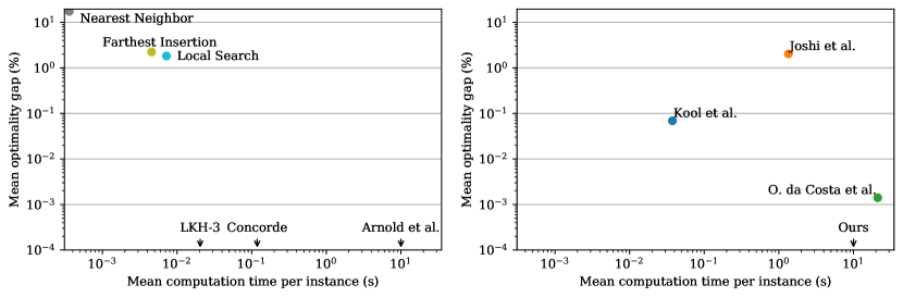
(a) TSP20

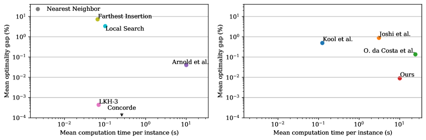
(b) TSP50

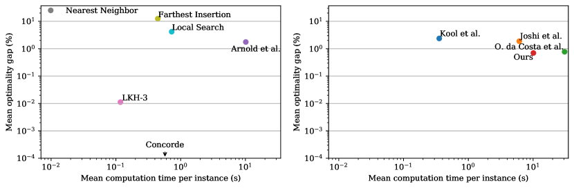
(c) TSP100

Figure 3: Mean optimality gap and computation time per instance for three increasingly difficult problem sets. The left plot shows non-learning based approaches, where the Nearest Neighbour heuristic, LKH-3, and Concorde typically form the Pareto front. The right plot shows learning based approaches, where Kool et al. (2018) and our approach form the Pareto front.

B.2 Convergence profile charts

We evaluate the solution quality, in terms of mean optimality gap and number of problems solved optimally, as a function of computation time over a fixed computation time. The resulting convergence profile provides a detailed view of how each approach trades off between solution quality and computation time. Figure 4 depicts convergence profiles for our approach and several recent learning based approaches, for models trained and evaluated on 20, 50, and 100-node problem instances. Computation time required to compute input features, evaluate a model, or to construct an initial solution is visible as a gap between the trace and the vertical axis, and is especially noticeable for Joshi et al. (2019).

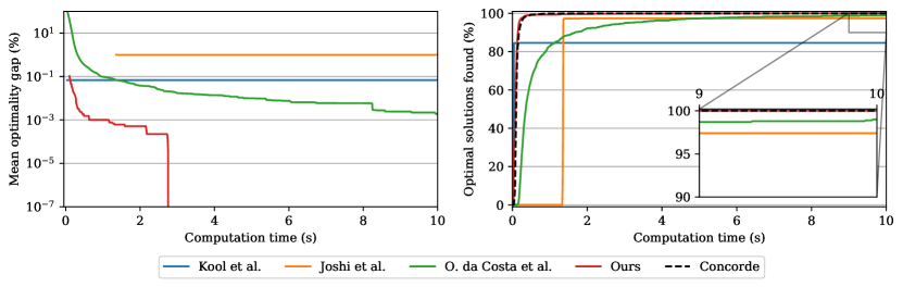
(a) TSP20

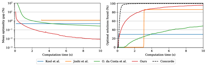
(b) TSP50

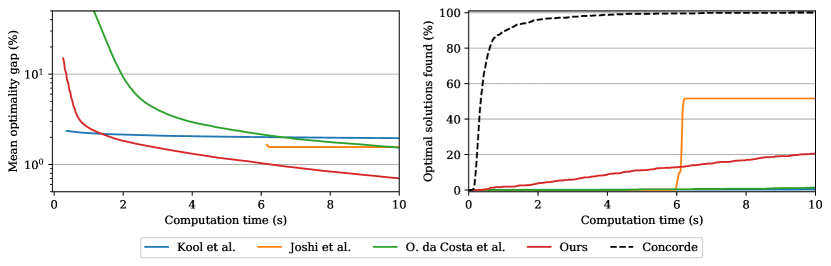
(c) TSP100

Figure 4: Solution quality as a function of computation time for three increasingly difficult problem sets, demonstrating that our method converges to optimal solutions at a faster rate than the evaluated learning based approaches. The left plot shows the mean optimality gap. The right plot shows the percentage of optimally solved problems.

Appendix C Generalization performance

C.1 Generalization to larger instances

Figure 5 depicts convergence profiles for the learning based approaches when generalizing from smaller problem instances to larger ones. The plots are arranged in order of increasing difference in size between the training and test problem sets.

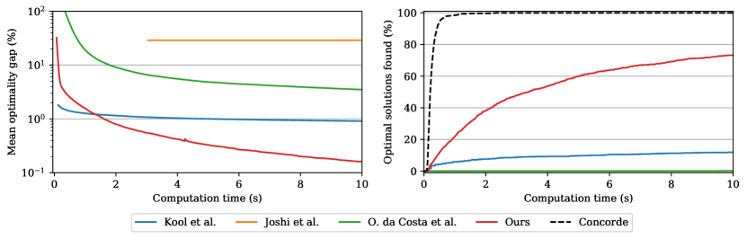
(a) Models trained on 20-node TSPs solving the TSP50 problem set.

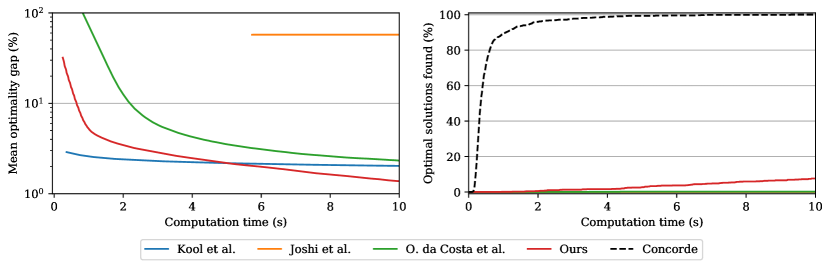
(b) Models trained on 50-node TSPs solving the TSP100 problem set.

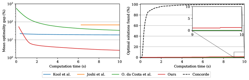
(c) Models trained on 20-node TSPs solving the TSP100 problem set.

Figure 5: Solution quality as a function of computation time for three increasingly difficult generalization tasks, demonstrating that our method is able to generalize from smaller to larger problem instances better than several learning based approaches. The left plot shows the mean optimality gap. The right plot shows the percentage of optimally solved problems.

C.2 Generalization to real-world instances

In many cases there may be insufficient examples of real-world problem instances to train a model, meaning it must be trained on synthetic data. Therefore, it is important to evaluate this “sim-to-real” transfer. Table 3 shows mean optimality gap and computation time for the evaluated learning based methods using models trained on random 100-node TSPs and evaluated on TSPLIB instances with 50 to 200 nodes and 2D Euclidean distances (29 instances).

Method	Kool et al.		Joshi et al.		O. da Costa et al.		Ours
Instance	Time (s)	Gap (%)	Time (s)	Gap (%)	Time (s)	Gap (%)	Time (s)	Gap (%)
eil51	0.125±0.000	1.628±0.125	3.026±0.012	8.339±0.000	28.051±0.040	0.067±0.097	10.074±0.068	0.000±0.000
berlin52	0.129±0.001	4.169±1.289	3.068±0.022	33.225±0.000	31.874±0.388	0.449±0.421	10.103±0.048	0.142±0.000
st70	0.200±0.001	1.737±0.093	4.037±0.009	24.785±0.000	23.964±0.122	0.040±0.085	10.053±0.078	0.764±0.000
eil76	0.225±0.000	1.992±0.004	4.303±0.021	27.411±0.000	26.551±0.065	0.096±0.237	10.155±0.067	0.163±0.000
pr76	0.226±0.002	0.816±0.130	4.378±0.023	27.793±0.000	39.485±0.152	1.228±0.908	10.049±0.023	0.039±0.000
rat99	0.347±0.000	2.645±0.103	5.559±0.016	17.633±0.000	32.188±0.064	0.123±0.000	9.948±0.013	0.550±0.000
kroA100	0.352±0.001	4.017±0.043	5.705±0.018	28.828±0.000	42.095±0.109	18.313±0.000	10.255±0.045	0.728±0.000
kroB100	0.352±0.002	5.142±0.269	5.712±0.018	34.686±0.000	35.137±0.078	1.119±0.060	10.317±0.150	0.147±0.000
kroC100	0.352±0.001	0.972±0.095	5.641±0.013	35.506±0.000	34.333±0.168	0.349±0.191	10.172±0.208	1.571±0.000
kroD100	0.352±0.001	2.717±0.327	5.621±0.024	38.018±0.000	25.772±0.090	0.866±0.447	10.375±0.155	0.572±0.000
kroE100	0.352±0.001	1.470±0.109	5.650±0.026	26.589±0.000	34.475±0.166	1.832±0.453	10.270±0.171	1.216±0.000
rd100	0.352±0.001	3.407±0.092	5.737±0.033	50.432±0.000	28.963±0.077	0.003±0.005	10.125±0.039	0.459±0.000
eil101	0.359±0.001	2.994±0.230	5.790±0.018	26.701±0.000	23.842±0.075	0.387±0.096	10.276±0.036	0.201±0.000
lin105	0.380±0.001	1.739±0.125	5.938±0.040	34.902±0.000	39.517±0.145	1.867±0.648	10.330±0.037	0.606±0.000
pr107	0.391±0.001	3.933±0.352	5.964±0.048	80.564±0.000	29.039±0.107	0.898±0.345	9.977±0.050	0.439±0.000
pr124	0.499±0.002	3.677±0.523	7.059±0.031	70.146±0.000	29.570±0.038	10.322±4.603	10.360±0.190	0.755±0.000
bier127	0.522±0.001	5.908±0.414	7.242±0.022	45.561±0.000	39.029±0.146	3.044±0.272	10.260±0.124	1.948±0.000
ch130	0.550±0.001	3.182±0.182	7.351±0.074	39.090±0.000	34.436±0.160	0.709±0.762	10.032±0.063	3.519±0.000
pr136	0.585±0.000	5.064±0.998	7.727±0.026	58.673±0.000	31.056±0.081	0.000±0.000	10.379±0.077	3.387±0.000
pr144	0.638±0.001	7.641±0.516	8.132±0.017	55.837±0.000	28.913±0.093	1.526±0.276	10.276±0.080	3.581±0.000
ch150	0.697±0.002	4.584±0.324	8.546±0.048	49.743±0.000	35.497±0.117	0.312±0.084	10.109±0.060	2.113±0.000
kroA150	0.695±0.001	3.784±0.336	8.450±0.017	45.411±0.000	29.399±0.059	0.724±0.198	10.331±0.281	2.984±0.000
kroB150	0.696±0.002	2.437±0.188	8.573±0.021	56.745±0.000	29.005±0.071	0.886±0.347	10.018±0.103	3.258±0.000
pr152	0.708±0.001	7.494±0.265	8.632±0.035	33.925±0.000	29.003±0.106	0.029±0.018	10.267±0.096	3.119±0.000
u159	0.764±0.001	7.551±1.581	9.012±0.019	38.338±0.000	28.961±0.096	0.054±0.000	10.428±0.078	1.020±0.000
rat195	1.114±0.003	6.893±0.505	11.236±0.028	24.968±0.000	34.425±0.054	0.743±0.312	12.295±0.087	1.666±0.000
d198	1.153±0.052	373.020±45.415	11.519±0.091	62.351±0.000	30.864±0.066	0.522±0.297	12.596±0.043	4.772±0.000
kroA200	1.150±0.000	7.106±0.391	11.702±0.036	40.885±0.000	33.832±0.402	1.441±0.068	11.088±0.075	2.029±0.000
kroB200	1.150±0.001	8.541±0.565	11.689±0.041	43.643±0.000	31.951±0.128	2.064±0.419	11.267±0.245	2.589±0.000
Mean	0.532±0.300	16.767±67.953	7.000±2.415	40.025±15.702	31.766±4.543	1.725±3.767	10.420±0.630	1.529±1.328

Table 3: Solution quality and computation time for for learning based methods using a model trained on random 100-node problems and evaluated on TSPLIB instances with 50 to 200 nodes and 2D Euclidean distances. Means and standard deviations are reported, calculated across 10 runs per problem instance. Pareto optimal values (i.e. faster or better solutions) are bolded.

Appendix D Analysis of additional input features

We evaluate the potential benefit of adding additional features to our regret approximation model. While more features can help produce better predictions, they come at the cost of additional computation time. We consider a total of ten additional features, described in Table 4. We use a Gaussian process-based surrogate model to conduct global sensitivity analysis (Gratiet et al., 2016) of the input features on the validation loss of the model after training. We assume that better regret predictions will equate to better guidance by the GLS algorithm, ultimately resulting in better performance to the problem sets.

Name	Description	Complexity
Node width	Perpendicular distance from a node to a line from the depot node through the centroid of the nodes (Arnold & Sörensen, 2019b).	$\Theta(n)$
Edge width	Absolute difference between the width of two nodes.	$\Theta(n^{2})$
Depot weight	Weight from a node to the depot node.	$\Theta(n)$
Neighbor rank	$k$ where node $j$ is the $k$-nearest neighbor of $i$. There are two features for a given edge, the rank of $i$ w.r.t. $j$ and the rank of $j$ w.r.t. $i$.	$\Theta(n^{2})$
30%-NN graph	If the edge is part of the $k$-nearest neighbor graph, where $k$ is 0.3$n$.	$\Theta(n^{2})$
20%-NN graph	If the edge is part of the $k$-nearest neighbor graph, where $k$ is 0.2$n$.	$\Theta(n^{2})$
10%-NN graph	If the edge is part of the $k$-nearest neighbor graph, where $k$ is 0.1$n$.	$\Theta(n^{2})$
MST	If the edge is part of the minimum spanning tree, calculated using Prim’s algorithm (Prim, 1957).	$\Theta(n^{2})$
NN solution	If the edge is part of solution constructed by the nearest neighbor heuristic.	$\Theta(n)$
NI solution	If the edge is part of solution constructed by the nearest insertion heuristic.	$\Theta(n^{3})$

Table 4: Summary of additional input features evaluated. While more features can help produce better predictions, and thus better guidance for the GLS algorithm, they come at the cost of additional computation time.

We semi-randomly sample 100 input feature sets using Latin hypercube sampling (McKay et al., 1979). We train a model using each of these feature sets for 35 epochs without early stopping and record the final validation loss. Using these results, we fit a Gaussian process to emulate the mapping between the feature set $F=\{f_{0},f_{1},\dots,f_{10}\}$, and the validation loss $l$ achieved by our model after training, where $f_{n}$ indicates whether or not feature $n$ is used. We then compute Monte-Carlo estimates of the main and total effects of each input feature on the model’s validation loss (Saltelli, 2002). Our implementation uses Emukit (Paleyes et al., 2019). Figure 6 depicts the estimated total effect for each input feature. Edge weight is the most important feature, followed by neighbor rank, depot weight, edge width, and node width. The remaining features have little to no importance.

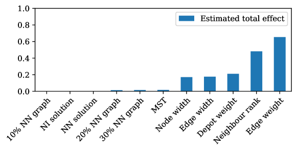
Figure 6: The estimated total effect of edge weight and ten additional features on model validation loss after training based on 100 randomly-sampled feature sets, using Gaussian process-based global sensitivity analysis. A small effect implies that the feature is not important when predicting regret, and vice-versa.

We train a model using these top five features on 20-node problems and compare its performance to the equivalent model using edge weight as the only feature when solving the 20, 50, and 100-node problem sets. The performance of both models at the computation time limit is shown in Table 5. While the model using additional input features produces slightly more accurate regret predictions, any benefit is cancelled out by the additional time required to compute these features. Note that the results are slightly different from those reported in Figure 5 due to different training hyperparameters.

Problem	Method	Optimality gap (%)	Optimal solutions (%)
TSP20	Local search only	1.824±3.252	54.7000
	Edge weight only	0.000±0.000	100.0000
	Top 5 features	0.000±0.003	99.9000
TSP50	Local search only	3.357±2.602	6.4000
	Edge weight only	0.082±0.254	82.1000
	Top 5 features	0.080±0.295	83.2000
TSP100	Local search only	4.169±2.046	0.3000
	Edge weight only	2.183±1.383	2.2000
	Top 5 features	2.228±1.421	2.2000

Table 5: Ablation analysis of our method using local search alone (no guidance), a model using edge weight alone, and model using additional features. Both models are trained on 20-node problems and evaluated on the 20, 50, and 100-node problem sets. The mean optimality gap and standard deviation, as well as the percentage of optimally solved problems are reported after 10 seconds of computation time per instance. While the model using additional input features produces slightly more accurate regret predictions, any benefit is cancelled out by the additional time required to compute these features.

References

- Accorsi et al. (2021) Luca Accorsi, Andrea Lodi, and Daniele Vigo. Guidelines for the computational testing of machine learning approaches to vehicle routing problems, 2021.
- Applegate et al. (2003) David Applegate, Robert Bixby, Vašek Chvátal, and William Cook. Implementing the Dantzig-Fulkerson-Johnson algorithm for large traveling salesman problems. Mathematical Programming, 97(1):91–153, 2003.
- Applegate et al. (2006) David Applegate, Robert Bixby, Vašek Chvatál, and William Cook. The Traveling Salesman Problem: A Computational Study. Princeton University Press, Princeton, NJ, 2006.
- Arnold & Sörensen (2019a) Florian Arnold and Kenneth Sörensen. Knowledge-guided local search for the vehicle routing problem. Computers & Operations Research, 105:32–46, 2019a.
- Arnold & Sörensen (2019b) Florian Arnold and Kenneth Sörensen. What makes a VRP solution good? The generation of problem-specific knowledge for heuristics. Computers & Operations Research, 106:280–288, 2019b.
- Bello et al. (2016) Irwan Bello, Hieu Pham, Quoc V Le, Mohammad Norouzi, and Samy Bengio. Neural combinatorial optimization with reinforcement learning. arXiv preprint arXiv:1611.09940, 2016.
- Bengio et al. (2021) Yoshua Bengio, Andrea Lodi, and Antoine Prouvost. Machine learning for combinatorial optimization: A methodological tour d’horizon. European Journal of Operational Research, 290(2):405–421, 2021.
- Cappart et al. (2021) Quentin Cappart, Didier Chételat, Elias Khalil, Andrea Lodi, Christopher Morris, and Petar Veličković. Combinatorial optimization and reasoning with graph neural networks. arXiv preprint arXiv:2102.09544, 2021.
- Croes (1958) G. A. Croes. A method for solving traveling-salesman problems. Operations Research, 6(6):791–812, 1958.
- da Costa et al. (2020) Paulo R de O da Costa, Jason Rhuggenaath, Yingqian Zhang, and Alp Akcay. Learning 2-opt heuristics for the traveling salesman problem via deep reinforcement learning. arXiv preprint arXiv:2004.01608, 2020.
- Dai et al. (2017) Hanjun Dai, Elias B. Khalil, Yuyu Zhang, Bistra Dilkina, and Le Song. Learning combinatorial optimization algorithms over graphs. In International Conference on Neural Information Processing Systems, pp. 6351–6361, 2017.
- Dantzig et al. (1954) G. Dantzig, R. Fulkerson, and S. Johnson. Solution of a large-scale traveling-salesman problem. Journal of the Operations Research Society of America, 2(4):393–410, 1954.
- Deudon et al. (2018) Michel Deudon, Pierre Cournut, Alexandre Lacoste, Yossiri Adulyasak, and Louis-Martin Rousseau. Learning heuristics for the TSP by policy gradient. In Integration of Constraint Programming, Artificial Intelligence, and Operations Research, pp. 170–181, 2018.
- Fu et al. (2021) Zhang-Hua Fu, Kai-Bin Qiu, and Hongyuan Zha. Generalize a small pre-trained model to arbitrarily large tsp instances, 2021.
- Gilmer et al. (2017) Justin Gilmer, Samuel S Schoenholz, Patrick F Riley, Oriol Vinyals, and George E Dahl. Neural message passing for quantum chemistry. In International Conference on Machine Learning, pp. 1263–1272. PMLR, 2017.
- Gratiet et al. (2016) Loïc Le Gratiet, Stefano Marelli, and Bruno Sudret. Metamodel-based Sensitivity Analysis: Polynomial Chaos Expansions and Gaussian Processes, pp. 1–37. Springer International Publishing, Cham, 2016.
- Hassin & Keinan (2008) Refael Hassin and Ariel Keinan. Greedy heuristics with regret, with application to the cheapest insertion algorithm for the TSP. Operations Research Letters, 36(2):243–246, 2008.
- Helsgaun (2009) Keld Helsgaun. General k-opt submoves for the Lin–Kernighan TSP heuristic. Mathematical Programming Computation, 1(2):119–163, 2009.
- Helsgaun (2017) Keld Helsgaun. An extension of the Lin-Kernighan-Helsgaun TSP solver for constrained traveling salesman and vehicle routing problems. Technical report, Roskilde University, 2017.
- Ioffe & Szegedy (2015) Sergey Ioffe and Christian Szegedy. Batch normalization: Accelerating deep network training by reducing internal covariate shift. In International Conference on Machine Learning, pp. 448–456. PMLR, 2015.
- Joshi et al. (2019) Chaitanya K Joshi, Thomas Laurent, and Xavier Bresson. An efficient graph convolutional network technique for the travelling salesman problem. arXiv preprint arXiv:1906.01227, 2019.
- Kingma & Ba (2014) Diederik P Kingma and Jimmy Ba. Adam: A method for stochastic optimization. arXiv preprint arXiv:1412.6980, 2014.
- Kool et al. (2018) Wouter Kool, Herke Van Hoof, and Max Welling. Attention, learn to solve routing problems! arXiv preprint arXiv:1803.08475, 2018.
- Kool et al. (2021) Wouter Kool, Herke van Hoof, Joaquim Gromicho, and Max Welling. Deep policy dynamic programming for vehicle routing problems, 2021.
- Kwon et al. (2021) Yeong-Dae Kwon, Jinho Choo, Byoungjip Kim, Iljoo Yoon, Youngjune Gwon, and Seungjai Min. Pomo: Policy optimization with multiple optima for reinforcement learning, 2021.
- Lin & Kernighan (1973) S. Lin and B. W. Kernighan. An effective heuristic algorithm for the traveling-salesman problem. Operations Research, 21(2):498–516, 1973.
- McKay et al. (1979) M. D. McKay, R. J. Beckman, and W. J. Conover. A comparison of three methods for selecting values of input variables in the analysis of output from a computer code. Technometrics, 21(2):239–245, 1979.
- Mnih et al. (2015) Volodymyr Mnih, Koray Kavukcuoglu, David Silver, Andrei A. Rusu, Joel Veness, Marc G. Bellemare, Alex Graves, Martin Riedmiller, Andreas K. Fidjeland, Georg Ostrovski, Stig Petersen, Charles Beattie, Amir Sadik, Ioannis Antonoglou, Helen King, Dharshan Kumaran, Daan Wierstra, Shane Legg, and Demis Hassabis. Human-level control through deep reinforcement learning. Nature, (508):529–533, 2015.
- Pacheco et al. (2021) Toni Pacheco, Rafael Martinelli, Anand Subramanian, Túlio A. M. Toffolo, and Thibaut Vidal. Exponential-size neighborhoods for the pickup-and-delivery traveling salesman problem. arXiv preprint arXiv:2107.05189, 2021.
- Padberg & Rinaldi (1990) Manfred Padberg and Giovanni Rinaldi. A branch-and-cut algorithm for the resolution of large-scale symmetric traveling salesman problems. Society for Industrial and Applied Mathematics, 33(1):60–100, 1990.
- Paleyes et al. (2019) Andrei Paleyes, Mark Pullin, Maren Mahsereci, Neil Lawrence, and Javier Gonzalez. Emulation of physical processes with emukit. In Second Workshop on Machine Learning and the Physical Sciences. NeurIPS, 2019.
- Paszke et al. (2019) Adam Paszke, Sam Gross, Francisco Massa, Adam Lerer, James Bradbury, Gregory Chanan, Trevor Killeen, Zeming Lin, Natalia Gimelshein, Luca Antiga, et al. Pytorch: An imperative style, high-performance deep learning library. In Advances in Neural Information Processing Systems, pp. 8026–8037, 2019.
- Potvin & Rousseau (1993) Jean-Yves Potvin and Jean-Marc Rousseau. A parallel route building algorithm for the vehicle routing and scheduling problem with time windows. European Journal of Operational Research, 66(3):331–340, 1993.
- Prim (1957) Robert C. Prim. Shortest connection networks and some generalizations. The Bell System Technical Journal, 36(6):1389–1401, 1957.
- Reddy (1977) Dabbala Raj Reddy. Speech understanding systems: Summary of results of the five-year research effort at Carnegie-Mellon University. Technical report, Carnegie Mellon University, 1977.
- Saltelli (2002) Andrea Saltelli. Making best use of model evaluations to compute sensitivity indices. Computer Physics Communications, 145(2):280–297, 2002.
- Smith (1999) Kate Smith. Neural networks for combinatorial optimization: A review of more than a decade of research. INFORMS Journal on Computing, 11(1):15–34, 1999.
- Vaswani et al. (2017) Ashish Vaswani, Noam Shazeer, Niki Parmar, Jakob Uszkoreit, Llion Jones, Aidan N Gomez, Łukasz Kaiser, and Illia Polosukhin. Attention is all you need. In Advances in Neural Information Processing Systems, pp. 5998–6008, 2017.
- Veličković et al. (2017) Petar Veličković, Guillem Cucurull, Arantxa Casanova, Adriana Romero, Pietro Lio, and Yoshua Bengio. Graph attention networks. arXiv preprint arXiv:1710.10903, 2017.
- Vinyals et al. (2015) Oriol Vinyals, Meire Fortunato, and Navdeep Jaitly. Pointer networks. arXiv preprint arXiv:1506.03134, 2015.
- Voudouris & Tsang (1996) Chris Voudouris and Edward Tsang. Partial constraint satisfaction problems and guided local search. Technical report, Department of Computer Science, University of Essex, 1996.
- Voudouris & Tsang (1999) Christos Voudouris and Edward Tsang. Guided local search and its application to the traveling salesman problem. European Journal of Operational Research, 113(2):469–499, 1999.
- Wang et al. (2019) Minjie Wang, Da Zheng, Zihao Ye, Quan Gan, Mufei Li, Xiang Song, Jinjing Zhou, Chao Ma, Lingfan Yu, Yu Gai, Tianjun Xiao, Tong He, George Karypis, Jinyang Li, and Zheng Zhang. Deep graph library: A graph-centric, highly-performant package for graph neural networks. arXiv preprint arXiv:1909.01315, 2019.
- Wu et al. (2020) Yaoxin Wu, Wen Song, Zhiguang Cao, Jie Zhang, and Andrew Lim. Learning improvement heuristics for solving routing problems. arXiv preprint arXiv:1912.05784, 2020.