Stability of Floquet Majorana box qubits

Abstract

In one-dimensional topological superconductors driven periodically with the frequency $\omega$, two types of topological edge modes may appear, the well-known Majorana zero mode and a Floquet Majorana mode located at the quasi-energy $\hbar\omega/2$. We investigate two Josephson-coupled topological quantum wires in the presence of Coulomb interactions, forming a so-called Majorana box qubit. An oscillating gate voltage can induce Floquet Majorana modes in both wires. This allows encoding 3 qubits in a sector with fixed electron parity. If such a system is prepared by increasing the amplitude of oscillations adiabatically, it is inherently unstable as interactions resonantly create quasi particles. This can be avoided by using instead a protocol where the oscillation frequency is increased slowly. In this case, one can find a parameter regime where the system remains stable.

Majorana zero modes (MZMs) arise at the edges of one-dimensional topological superconductor (TS) [1]. A pair of MZMs can encode a qubit. MZMs allow to store quantum information non-locally, and are thus protected against local noise. In combination with their non-Abelian braiding statistics [2, 3], MZMs are promising candidates for topological quantum computation. Such systems can be realized in different physical setups, such as semiconducting quantum wires with strong spin-orbit coupling or from topological insulators, proximity coupled to conventional superconductors [4, 5, 6, 7, 8, 9, 10, 11].

Two Majoranas at the ends of a single quantum wire, however, do not define a useful qubit. In this case, the quantum information is encoded in the electron number parity of the system. It is very difficult to create coherent superpositions of such states and, furthermore, if the system is not grounded, the long-ranged Coulomb interaction leads to an energetic splitting between the two parity states. Therefore, a different setup - the Majorana box qubit - has been introduced [12, 13, 14, 11]. As shown in Fig. 1, two topological superconducting quantum wires on a floating superconducting island are coupled by Josephson junctions. Charging one wire relative to the other costs a finite energy. Due to this charging energy, the four-dimensional low-energy Hilbert space splits into two sectors with even and odd parity. Thus one obtains a single qubit, which can be embedded in larger quantum circuits [13].

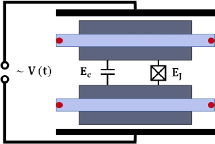
Figure 1: Schematic of the Floquet Majorana Box Qubit: Two topological superconducting nanowires (light blue) proximity coupled to two bulk superconductors (dark blue).The bulk superconductors are Josephson coupled with energy $E_{J}$ and in the Coulomb blockage regime with large $E_{c}$. The bulk superconductors are driven by a capacitively coupled voltage $V(\tau)$.

In this paper, we combine the idea of a Majorana box qubit with another powerful concept. In periodically driven systems, one can realize topological phases with no equilibrium equivalent [15, 16, 17, 18, 19, 20, 21, 22, 23, 24, 25]. It has been shown that driving a single topological superconductor periodically leads to the emergence of an extra pair of topologically protected Majorana modes [26, 27, 28, 29, 30, 31] or even more Majorana states, when multiple incommensurate driving frequencies are used [32]. Similarly to MZMs in static systems, Floquet Majorana modes, also called Majorana $\pi$ modes (MPM), are localized to the ends of the system. However, their quasi-energy is $\pi\frac{\hbar}{T}=\frac{\hbar\omega}{2}$, where $\omega=\frac{2\pi}{T}$ is the driving frequency and $T$ the period of driving. As Floquet Majoranas and ordinary MZMs have different quasi-energies, they do not hybridize.

This allows for a topologically protected braiding operation [33] even in a one-dimensional wire, given that the time-dependent Hamiltonian is nearly perfectly periodic in time.

We will show how this principle can be used to construct a “Floquet Majorana box” by simply driving the system with an AC voltage which is applied via gates to the two superconducting islands as shown in Fig. 1.

The device hosts a total of three logical qubits in each subspace of fixed electron parity. A similar device based on the corner modes of a second-order topological superconductor was recently considered by Bomantara and Gong [34]. They showed that such a setup allows for all Clifford gate operations, both for one and two qubits, in a topologically protected way and can be used for braiding experiments.

The main goal of our study is to explore interaction effects, which are unavoidable in a device based on Coulomb blockade. We will first derive an effective low-energy theory for the Floquet Majorana box qubit which allows us to study the emergence of Floquet Majoranas. Using perturbation theory, we explore interaction effects and show that the stability of the system depends decisively on the preparation protocol of the driven system.

Model: To obtain a minimal model for the physics of the device shown in Fig. 1, we consider two Kitaev chains, $\alpha=1,2$, coupled to two superconducting islands.

$$H=\frac{E_{c}}{2}\hat{Q}^{2}-E_{J}\cos(\hat{\phi})+\hat{Q}V(\tau)-\sum_{i,\alpha}\mu c_{i,\alpha}^{\dagger}c_{i,\alpha}+\sum_{i,\alpha}\left(-\frac{t}{2}c_{i,\alpha}^{\dagger}c_{i+1,\alpha}+\frac{\Delta}{2}e^{(-1)^{\alpha}i\hat{\phi}/2}c_{i,\alpha}^{\dagger}c_{i+1,\alpha}^{\dagger}+h.c.\right)$$ (1)

Here $\hat{\phi}=\hat{\phi}_{1}-\hat{\phi}_{2}$ is the phase difference of the two superconducting islands and the operator $\hat{Q}=\hat{Q}_{1}-\hat{Q}_{2}$ counts the difference in the number of cooper pairs on the two islands. $E_{c}$ is the charging energy associated with this charge imbalance and $E_{J}$ denotes the Josephson coupling arising from Cooper pair tunneling, with $[\hat{Q},e^{\pm i\hat{\phi}/2}]=\pm e^{\pm i\hat{\phi}/2}$. The system is driven by a time-dependent ac voltage, $V(\tau)=V_{0}\cos(\omega\tau)$ where we denote time by $\tau$. For simplicity, we model the interactions here by the charging term $\frac{E_{c}}{2}\hat{Q}^{2}$ only (omitting further interactions both within each Majorana chain and between the chains and the superconducting islands), but we will argue below that all qualitative results remain valid when further weak interactions are included. Furthermore, the global charging energy $Q_{\rm{tot}}^{2}/(2C)$ has been omitted as we consider only processes where the total charge $Q_{\rm{tot}}$ is conserved.

We assume that all energy scales associated with the quantum wires and the driving frequency $\omega$ are much smaller than the driving amplitude $V_{0}$ and the energy scales associated with the large superconducting islands, $\omega,\Delta,t,\mu\ll E_{c}\ll E_{J},V_{0}$. The limit $E_{c}\ll E_{J}$ is necessary for the operation of the box qubit, exponentially suppressing the relative charging energy between the quantum wires and the sensitivity to charge noise [35, 13]. Since $E_{c}\ll E_{J}$, phase fluctuations are small, $\cos\hat{\phi}\approx 1-\frac{\hat{\phi}^{2}}{2}$, and the superconducting islands are well described by a time-dependent harmonic oscillator

$$H_{SC}(\tau)=\frac{E_{c}}{2}\hat{Q}^{2}+\frac{E_{J}}{2}\hat{\phi}^{2}+\hat{Q}V(\tau).$$ (2)

To derive an effective low-energy Hamiltonian for the driven Kitaev chains, we apply three unitary transformations (see Appendix A for details): We shift the $\hat{Q}$ coordinate of the harmonic oscillator to absorb the linear term $\hat{Q}V(\tau)$ by the unitary $U_{1}(\tau)=e^{-i\hat{\phi}V(\tau)/(2E_{c})}$. The resulting time-dependence of $\hat{Q}$ induces a time dependent phase, $\hat{\phi}\sim\partial_{\tau}Q/E_{J}$ , which we eliminate by a second transformation $U_{2}=e^{-i\hat{Q}\partial_{\tau}V(\tau)/(4E_{J}E_{c})}$. Finally, we use a Schrieffer-Wolff transformation $U_{3}=e^{-i\hat{Q}\frac{\Delta}{8E_{J}}T}$ to eliminate perturbatively transitions to excited states of $H_{SC}$ triggered by $e^{\pm i\hat{\phi}/2}$ in Eq. (1). All approximations are well-controlled for $\Delta\ll E_{J}$, $E_{c}\ll E_{J}$, and $V_{0}\ll\frac{E_{c}E_{J}}{\omega}$, see App. A. We thus arrive at the time-dependent low-energy Hamiltonian

$$H_{\rm eff}(\tau) =-\sum_{i,\alpha}\mu c^{\dagger}_{i,\alpha}c_{i,\alpha}+\sum_{i,\alpha}\left(-\frac{t}{2}c^{\dagger}_{i,\alpha}c_{i+1,\alpha}+\frac{\Delta}{2}e^{-(-1)^{\alpha}i\frac{\dot{V}(\tau)}{2E_{c}E_{J}}}c^{\dagger}_{i,\alpha}c^{\dagger}_{i+1,\alpha}+h.c.\right)+\frac{\Delta^{2}}{32E_{J}}T^{2},$$ (3)

$$T =ie^{-i(-1)^{\alpha}\frac{\dot{V}(\tau)}{2E_{c}E_{J}}}\sum_{i,\alpha}c^{\dagger}_{i,\alpha}c^{\dagger}_{i+1,\alpha}+h.c.$$

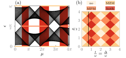
Figure 2: (a) Floquet spectrum as a function of the static chemical potential $\mu$ ($N=60$, $\delta\mu=3\pi$, $t=\pi$, $T=1.4$, $N_{\text{steps}}=100$, $\Delta=-\pi$). The Majorana zero mode (MZM) and the Majorana $\pi$ modes (MPM) are depicted in light orange and orange, respectively. Areas of co-existing MZM and MPM are shaded in red. (b) Phase diagram of the driven Kitaev chain as function of $\frac{t}{\omega}=\frac{\Delta}{\omega}$ and $\frac{\mu}{\omega}$. It shows the four different phases: trivial, only MZM, only MPM and both modes.

We first study the non-interacting part of $H_{\rm eff}$ considering the small interaction effects encoded in the last term of Eq. (3) only later. The time-dependent phase can be absorbed by a gauge transformation and rewritten as a time-dependent chemical potential

$$H^{0}_{\text{eff}}= \sum_{i,\alpha}-\left(\mu-(-1)^{\alpha}\delta\mu\,\cos(\omega\tau)\right)c^{\dagger}_{i,\alpha}c_{i,\alpha}$$

$$\quad-\frac{t}{2}c^{\dagger}_{i,\alpha}c_{i+1,\alpha}+\frac{\Delta}{2}c^{\dagger}_{i,\alpha}c^{\dagger}_{i+1,\alpha}+h.c.$$ (4)

with $\delta\mu=V_{0}\frac{\omega^{2}}{E_{c}E_{J}}$ for an oscillating gate voltage, $V(\tau)=V_{0}\cos(\omega\tau)$. The spectrum and the topological Floquet phases of this non-interacting Hamiltonian, which have been studied before [33, 26, 27], are shown in Fig. 2. Since energy is only conserved modulo the driving frequency $\omega$, this so called quasi-energy is shown in the Floquet spectrum in Fig. 2. Importantly, one obtains phases (red shaded regions in Fig. 2a) where Majorana zero modes and Floquet Majorana modes at quasi-energy $\pi/T=\omega/2$ coexist. The spectrum was obtained numerically by calculating the Floquet time evolution operator $U_{F}$ for a finite-size system over one period $T$ by a Suzuki-Trotter decomposition using the Floquet Hamiltonian $H_{F}=i\log(U_{F})/T$. Equivalently, the spectrum can be obtained by solving the Floquet matrix, see App. D. The phase diagram of Fig. 2 is obtained from the topological charges of the bulk bands, see [26, 33].

Importantly, the Floquet spectrum is not sufficient to describe the system, as it does not specify the many-body (Floquet-) state, which may depend on the way the system is prepared. We first consider the standard setup for adiabatic state preparation by assuming that system is initially in the ground state of the Hamiltonian (1) with $V_{0}=0$. The oscillating gate voltage is then switched on slowly. In the following, we will focus on the bulk problem but we have checked numerically that the same physics also governs finite-size system. The initial state (with $V(\tau)=0$ ) is the ground state $|GS\rangle$, and the excited states $a^{\dagger}_{k}|GS\rangle$ have positive energies, $E_{k}\geq 0$, while $a_{k}|GS\rangle=0$. Within the Bogoliubov theory, one formally introduces negative energy states using $E_{k}a_{k}^{\dagger}a_{k}=-E_{k}a_{k}a^{\dagger}_{k}$. We call these negative energies $-E_{k}$ ‘Bogoliubov shadows’ to emphasize that the physical excitations have positive energies.

Within the Floquet formalism, however, energies are only defined modulo $\omega$. Thus it is not possible to distinguish physical excitations and their Bogoliubov shadows simply by their quasi-energy. Fig. 3a shows the spectrum of the undriven system folded into the first Floquet zone, $0\leq E<\omega$. Here the red line is the physical excitation, the blue dashed line the Bogoliubov shadow $-E_{-k}+\omega$ projected into the Floquet zone $0<E\leq\omega$. The modes touch at $k_{0}$ with $E_{k_{0}}=-E_{-k_{0}}+\omega$, i.e., $E_{k_{0}}=\omega/2$. When the oscillating field is switched on, the modes hybridize, which is a necessary condition to create the $\pi$ Majorana mode at this quasi-energy, $\omega/2=\pi/T$.

Importantly, one has to track which of the hybridized modes describes a physical excitation and which describes only its Bogoliubov shadow. We can simply use adiabatic continuity to track whether an excitation is physical or a shadow excitation, see App. D. This is shown in Fig. 3b, where physical excitations are again shown in dark red while Bogoliubov shadows are depicted as dashed lines in light blue. For $k<k_{0}$ ($k>k_{0}$) the mode with quasi-energy smaller (larger) than $\omega/2$ has to be identified as a physical excitation shown in dark red. At the crossing point $k_{0}$ a singularity develops leading to a jump in the nature of the excitation (and the excitation energy), see Fig. 3. An alternative, but equivalent, way to describe the same physics is to investigate the nature of the many-particle state created by the adiabatic evolution. The BCS wave function is written as $\prod_{k}(u_{k}+v_{k}a_{k}^{\dagger}a^{\dagger}_{-k})|0\rangle$. Here the parameters $u_{k}$ and $v_{k}$ develop a singularity at $k=k_{0}$ where they exchange their role.

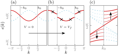
Figure 3: Bulk Floquet spectrum as a function of momentum $k$ ($\mu=0.1\pi$, $t=-\Delta=\pi$, $\omega=\pi$, $\delta\mu_{f}=0.2$) prepared by adiabatically switching on the oscillating voltage $V$. A band gap opens at energy $\omega/2$ (panel (a): undriven, panel (b): driven system). The quasi-energy of physical excitation, $\tilde{a}_{k}^{\dagger}\ket{\text{GS}}$, is marked as a red solid line, their ‘Bogoliubov shadow’ as a blue dashed line. As physical excitations transform always into physical excitations under adiabatic evolution, the red solid line develops a jump at $\pm k_{0}$. This adiabatic evolution is shown in an enlarged view in panel (c). The resulting state is highly unstable as it allows the resonant creation of four quasi particles with total quasi-energy $\omega$. The 4 crosses give an example of such a process.

To investigate the stability of the resulting state, we expand the interaction (last term in Eq. (3)) in creation and annihilation operators of the Floquet-Bogoliubov eigenmodes, $\tilde{a}^{\dagger}_{\nu}$ with quantum numbers $\nu$ (with $\nu=k$ for the translationally invariant bulk system considered above). The interactions may trigger the creation of four quasi- particle due to the term

$$\Delta H_{\text{int}}=\sum V^{m}_{\nu_{1},\nu_{2},\nu_{3},\nu_{4}}e^{im\omega\tau}\tilde{a}^{\dagger}_{\nu_{1}}\tilde{a}^{\dagger}_{\nu_{2}}\tilde{a}^{\dagger}_{\nu_{3}}\tilde{a}^{\dagger}_{\nu_{4}},$$ (5)

where $V^{m}_{\nu_{1},\nu_{2},\nu_{3},\nu_{4}}\sim\Delta^{2}/E_{J}$ is defined in App. B. The corresponding creation rate of quasi particles can then be estimated using Fermi’s golden rule

$$\gamma_{qp}=4\frac{2\pi}{\hbar}\sum_{\nu_{i},m}\delta(E_{\nu_{1}}+E_{\nu_{2}}+E_{\nu_{3}}+E_{\nu_{4}}+m\omega)|V^{m}_{\nu_{1}\nu_{2}\nu_{3}\nu_{4}}|^{2},$$ (6)

where $E_{\nu_{i}}\geq 0$ are excitation energies obtained by diagonalizing the non-interacting Bogoliubov-Floquet system and the factor $4$ originates from the fact that four quasi-particles are created by the interaction. In our numerical calculations described below for finite-size systems with a discreet spectrum, we broaden the $\delta$-function slightly by a box function of width $\Delta E$ to account for finite-lifetime effects, not captured by the golden-rule formula.

Applying Eq. (6) to the bulk energies, one realizes immediately that the jump in the quasi-energy of physical excitations enforces physical excitation both below and above $\frac{\omega}{2}$ (depicted in red in Fig. 3). With the discontinuity, there is an abundance of resonant quasi-particle creation processes of the type depicted by four crosses in Fig. 3, namely when quasi-energies add up to (multiples of) $\omega$. In the bulk system, the total rate $\gamma_{qp}$ even diverges logarithmically due to processes occurring close to the location of the jump, $k_{0}$. We, therefore, conclude that the system is completely unstable when one prepares a system with $\pi$ Majoranas simply by adiabatically switching on of the oscillating gate voltage. We expect that a similar statement applies to a wide range of models with $\pi$ Majoranas which naturally emerge from the crossing of Bogoliubov modes at energy $\omega/2$.

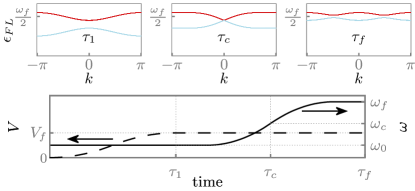
Figure 4: A ‘frequency sweep protocol’ can be used to create a stable topological Floquet state. First, the amplitude of the oscillating voltage is increased slowly using a small frequency $\omega_{0}$. Then the frequency is increased up to $\omega_{f}$. At $\tau=\tau_{c}$ one enters the topological phase ($\mu=0.1\pi$, $t=-\pi$, $\Delta=\pi$, $V_{f}=0.2$, $\omega_{0}=0.8\pi$, $\omega_{c}=0.9\pi$, $\omega_{f}=\pi$). The Floquet spectra for $\tau=\tau_{1}$, $\tau_{c}$ and $\tau_{f}$ are shown on top. The final Floquet spectrum is identical to the one shown in Fig. 3, but differs by the identification of physical excitations (red) vs. Bogoliubov shadows (blue).

Luckily, one can avoid this instability using a different preparation protocol, sketched in Fig. 4. The main idea is simply to avoid entering the topological Floquet phase directly by ramping up the oscillating field. Instead, we choose initially a frequency smaller than the band gap of the system while increasing the amplitude of the drive. Thus we avoid crossings of excitation energies and Bogoliubov shadows while preparing a non-topological Floquet state. Only at a second step, we slowly increase the frequency to reach the Floquet phase. Level repulsion ensures that one never obtains a crossing of excitation- and shadow modes. Instead, they only touch at the quantum critical point (QCP), see Fig. 4. Close to this point quasi-particle excitations are created by the Kibble-Zurek mechanism [36, 37, 38, 39]. Using the Landau-Zener formula for the Dirac Hamiltonian $m(t)\sigma_{z}+vk\sigma_{x}$, we estimate the density $n_{\text{KZ}}$ of these quasi particles by $n_{\text{KZ}}=\frac{\sqrt{\partial_{t}m}}{v}$[40, 41]. For a system size of 10 in units of the correlation length $m/v$, one can easily reach a regime where in total less than one quasi particle is created for $\partial_{t}m<0.01\,m^{2}$.

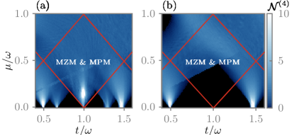
Figure 5: Normalized phase space density $\mathcal{N}^{(4)}=\frac{1}{N^{4}}\sum_{\nu_{i},m}\delta(E_{\nu_{1}}+E_{\nu_{2}}+E_{\nu_{3}}+E_{\nu_{4}}+m\omega)$ for the creation of four quasi particles out of the vacuum ($N=20$, $\delta E=0.02$, $t=-\Delta=\pi,\delta\mu=1$) Left: The Floquet state is prepared by adiabatically switching on the oscillating field. In this case the topological phase located inside the square is always unstable. Right: Preparation by the frequency-sweep protocol of Fig. 4 (right). Here large parts of the topological phase remain stable as indicated by the black color.

With this protocol, the resulting Floquet phase is much more long-lived. In Fig. 5 we show the phase space for the spontaneous creation of four quasi particles out of the vacuum for both types of protocols for a finite-size system. The topological Floquet phase is always unstable if the state is prepared simply by an increase of the oscillating voltage. In contrast, there is a wide range of parameters where the topological phase is stable to leading order in the interaction if one uses the frequency-sweep protocol of Fig. 4. This analysis holds both for the long-ranged interactions derived in Eq. (3) and for short-ranged interactions, see App. C for a numerical evaluation of the quasi-particle creation rate $\gamma_{qp}$, Eq. (6). We have checked that the region of stability is not enlarged when one considers only momentum-conserving bulk processes. As there is gap in the total 4-particle density of states, the frequency-sweep protocol is furthermore stable against weak spatial disorder. Possible processes of 4th and higher order in the interactions, which involve the simultaneous creation of six or more quasi particles, may still exist but their prefactors will be strongly suppressed.

Conclusion: We have shown that by simply using an oscillating gate voltage, one can boost a Majorana box qubit into its Floquet version, thus increasing the number of logical qubits (in the fixed parity sector) from 1 to 3 combining Majorana zero modes and Majorana $\pi$ modes. Just increasing the oscillating field creates, however, a state which is completely unstable in the presence of interactions. To avoid this, one has to use a protocol that takes a detour: one first creates a non-topological Floquet state before entering the topological Floquet phase. This can, e.g., be realized by a frequency sweep.

A Floquet Majorana box qubit provides with its three qubits a rich playground for quantum operations as outlined by Bomantara and Gong [34]. Using a tunnel coupling of the edge modes via gated quantum dots one can realize a full set of Clifford gates, perform two-qubit operations with a help of an ancilla qubit, and test the braiding statistics of Majorana modes.

To summarize, our work shows that such Floquet devices can be operated despite the presence of interactions.

Acknowledgements: We acknowledge funding from the German Research Foundation (DFG) through CRC 183 (project number 277101999, A01) and – under Germany’s Excellence Strategy – by the Cluster of Excellence Matter and Light for Quantum Computing (ML4Q) EXC2004/1 390534769. Furthermore, A.M. thanks the BCGS (Bonn-Cologne Graduate School of Physics and Astronomy) for support. E.B. acknowledges support from the Israel Science Foundation Quantum Science and Technology (grant no. 2074/19) and from a research grant from Irving and Cherna Moskowitz.

Appendix A Effective low-energy Hamiltonian

In the following, we show how an effective low-energy Hamiltonian can be obtained starting from Eq. (1) of the main text. We first apply the harmonic oscillator approximation $-E_{J}\cos\hat{\phi}\approx E_{J}(-1+\frac{1}{2}{\hat{\phi}}^{2})$ in the limit $E_{J}\gg E_{c}$ such that $\hat{\phi}$ is pinned to one of the minima of $\cos(\hat{\phi})$ and weakly fluctuates around the minimum. We then apply a series of unitary transformations to the Hamiltonian

$$H_{0}(\tau) =\frac{E_{c}}{2}\hat{Q}^{2}+\frac{E_{J}}{2}{\hat{\phi}}^{2}+\hat{Q}V(\tau)+\frac{\Delta}{2}\left(\sum_{i}c^{\dagger}_{i}c^{\dagger}_{i+1}e^{-i\hat{\phi}/2}+h.c.\right),$$ (7)

where we omitted in Eq. (7) all terms from Eq. (1) of the main text not affected by the transformations considered below. Furthermore, we consider only one of the chains (the result can easily be generalized to the two chain case).

To eliminate the time-dependent term linear in $\hat{Q}$, we apply the transformation $U_{1}(\tau)=e^{-i\hat{\phi}V(\tau)/(2E_{c})}$ and arrive at

$$H_{1}(\tau) =U^{\dagger}_{1}(\tau)H_{0}(\tau)U_{1}(\tau)-iU^{\dagger}_{1}(\tau)\partial_{\tau}U_{1}(\tau)$$

$$=\frac{E_{c}}{2}\hat{Q}^{2}+\frac{E_{J}}{2}\hat{\phi}^{2}+\frac{\Delta}{2}\left(\sum_{i}c^{\dagger}_{i}c^{\dagger}_{i+1}e^{-i\hat{\phi}/2}+h.c.\right)-\hat{\phi}\frac{\dot{V}(\tau)}{2E_{c}}+\text{const.}.$$ (8)

Now we eliminate the offset in $\hat{\phi}$ with a second transformation $U_{2}(\tau)=e^{-i\hat{Q}\frac{\dot{V}(\tau)}{4E_{c}E_{J}}}$ and obtain

$$H_{2}(\tau) =U^{\dagger}_{2}(\tau)H_{1}(\tau)U_{2}(\tau)-iU_{2}^{\dagger}(\tau)\partial_{\tau}U_{2}(\tau)$$

$$=\frac{E_{c}}{2}\hat{Q}^{2}+\frac{E_{J}}{2}\hat{\phi}^{2}+\frac{\Delta}{2}\left(\sum_{i}c^{\dagger}_{i}c^{\dagger}_{i+1}e^{-i(\hat{\phi}/2+\frac{\dot{V}(\tau)}{2E_{c}E_{J}})}+h.c.\right)-\hat{Q}\frac{V^{\prime\prime}(\tau)}{4E_{c}E_{J}}+\text{const.}.$$ (9)

Hereafter, we simply neglect the tiny term proportional to $\frac{V^{\prime\prime}(\tau)}{E_{c}E_{J}}\sim\frac{\omega^{2}V_{0}}{E_{c}E_{J}}\ll\omega\ll E_{c},E_{J}$. Next we expand $e^{-i\hat{\phi}/2}\approx 1-i\frac{\hat{\phi}}{2}$ and obtain

$$H_{3}(\tau) =\frac{E_{c}}{2}\hat{Q}^{2}+\frac{E_{J}}{2}\hat{\phi}^{2}+\frac{\Delta}{2}\left(\sum_{i}c^{\dagger}_{i}c^{\dagger}_{i+1}e^{-i\frac{\dot{V(\tau)}}{2E_{c}E_{J}}}+h.c.\right)-\frac{\Delta}{4}T\hat{\phi}+\text{const.}$$ (10)

with

$$T=i\left(e^{-i\frac{\dot{V}(\tau)}{2E_{c}E_{J}}}\sum_{i}c^{\dagger}_{i}c^{\dagger}_{i+1}-e^{i\frac{\dot{V}(\tau)}{2E_{c}E_{J}}}\sum_{i}c_{i+1}c_{i}\right).$$ (11)

The displacement of $\hat{\phi}$ is eliminated by a last transformation $U_{3}=e^{-i\hat{Q}\frac{\Delta}{8E_{J}}T}$. Since $U_{3}$ does not commute with the Kitaev Hamiltonian $H_{k}=\mu\sum_{i}c^{\dagger}_{i}c_{i}-\sum_{i}\left(\frac{t}{2}c^{\dagger}_{i}c_{i+1}+\frac{\Delta}{2}c^{\dagger}_{i}c^{\dagger}_{i+1}e^{-i\frac{\dot{V}(\tau)}{2E_{c}E_{J}}}+h.c.\right)$, we again include all terms in the Hamiltonian $\tilde{H}_{3}$

$$H_{4}(\tau) =U^{\dagger}_{3}(\tau)\tilde{H}_{3}(\tau)U_{3}(\tau)-iU_{3}^{\dagger}(\tau)\partial_{\tau}U_{3}(\tau)$$

$$=\frac{E_{c}}{2}\hat{Q}^{2}+\frac{E_{J}}{2}\hat{\phi}^{2}+H_{k}+\frac{\Delta^{2}}{32E_{J}}T^{2}+\frac{\Delta}{8E_{J}}[T,H_{k}]\hat{Q}+\mathcal{O}(\frac{1}{E_{J}^{2}})+\text{const.}.$$ (12)

We first neglect the terms of order $\frac{1}{E_{J}^{2}}$. The fifth term correspond to a small shift in $\hat{Q}$ which is of order $\sim\frac{\Delta^{2}}{E_{J}E_{c}}\ll E_{c}$, and thus can be neglected as well. Finally, we arrive at the low energy Hamiltonian $H_{\rm eff}$ (Eq. 3 in the main text)

$$H_{\rm eff}=\mu\sum_{i}c^{\dagger}_{i}c_{i}-\frac{t}{2}\sum_{i}c^{\dagger}_{i}c_{i+1}+\frac{\Delta}{2}e^{-i\frac{\dot{V}(\tau)}{2E_{c}E_{J}}}\sum_{i}c^{\dagger}_{i}c^{\dagger}_{i+1}+h.c.+\frac{\Delta^{2}}{32E_{J}}T^{2}.$$ (13)

Appendix B Floquet Fermi Golden Rule

To study the interaction effects, we look at the Floquet Fermi Golden rule [42, 43, 44]. First the creation (annihilation) operators $c^{\dagger}_{i}$ ($c_{i}$) are expressed in terms of the Floquet operators $\tilde{a}^{\dagger}_{\nu}$ ($\tilde{a}_{\nu}$) where $\tilde{a}^{\dagger}_{\nu}(\tau)\ket{0}=\ket{\phi_{\nu}(\tau)}$ creates a fermion in a Floquet eigenstate. Here $\ket{0}$ is the quasi-particle vacuum. We use that the single-particle Floquet eigenstates of our Hamiltonian $\ket{\phi_{\nu}(\tau)}$ at equal times form a complete set in the physical Hilbert space $\mathbb{1}=\sum_{\nu}\ket{\phi_{\nu}(\tau)}\bra{\phi_{\nu}(\tau)}$, where the sum runs only over states of the first Floquet zone. Therefore,

$$c_{j}^{\dagger}\ket{0}=\sum_{\nu}\ket{\phi_{\nu}(\tau)}\bra{\phi_{\nu}(\tau)}\ket{j}=\sum_{\nu}\bra{\phi_{\nu}(\tau)}\ket{j}\tilde{a}^{\dagger}_{\nu}(\tau)\ket{0}$$ (14)

and $c^{\dagger}_{j}=\sum_{\nu}\bar{\phi}_{\nu}(t,j)\tilde{a}^{\dagger}_{\nu}(\tau)$ with $\bar{\phi}_{\nu}(t,j)=\bra{\phi_{\nu}(\tau)}\ket{j}$. Now we can use the mode expansion of Floquet states $\ket{\phi_{\nu}(\tau)}=\sum_{n}e^{-in\omega\tau}\ket{\phi_{\nu}^{n}}$ and see that the Floquet operators have an explicit time dependence in the Schrödinger picture. However, we are looking for an expression for the creation (annihilation) operators in terms of the Floquet operators. Therefore, let us expand the $\bar{\phi}_{\nu}(t,i)$ and we get with $\bar{\phi}_{\nu}^{n}(j)=\bra{\phi^{n}_{\nu}}\ket{j}$:

$$c^{\dagger}_{j}=\sum_{\nu}e^{in\omega\tau}\bar{\phi}_{\nu}^{n}(j)\tilde{a}^{\dagger}_{\nu}(\tau)$$ (15)

with $\tilde{a}^{\dagger}_{\nu}(\tau)=e^{i\epsilon_{\nu}\tau}\tilde{a}^{\dagger}_{\nu}$. Now we can write

$$A(i\rightarrow f,\tau) =\bra{\psi_{f}(\tau)}U(0,\tau)\ket{\psi_{i}(\tau=0)}$$ (16)

$$=-\frac{i}{\hbar}\int_{0}^{\tau}d\tau^{\prime}\bra{\psi_{f}(0)}U(\tau^{\prime},0)\Delta H_{\text{int}}U(0,\tau^{\prime})\ket{\psi_{i}(0)}$$

$$=-\frac{i\Delta^{2}}{32\hbar E_{J}}\sum_{j,k}\sum_{n_{1},n_{2},n_{3},n_{4}}\sum_{\nu_{1},\nu_{2},\nu_{3},\nu_{4}}\int_{0}^{\tau}d\tau^{\prime}e^{i(n_{1}+n_{2}+n_{3}+n_{4})\omega\tau^{\prime}}e^{i(\epsilon_{\nu_{1}}+\epsilon_{\nu_{2}}+\epsilon_{\nu_{3}}+\epsilon_{\nu_{4}})\tau^{\prime}}$$

$$\times\bar{\phi}_{\nu_{1}}^{n_{1}}(j)\bar{\phi}_{\nu_{2}}^{n_{2}}(j+1)\bar{\phi}_{\nu_{3}}^{n_{3}}(k)\bar{\phi}_{\nu_{4}}^{n_{4}}(k+1)\bra{\psi_{f}(0)}\tilde{a}^{\dagger}_{\nu_{1}}\tilde{a}^{\dagger}_{\nu_{2}}\tilde{a}^{\dagger}_{\nu_{3}}\tilde{a}^{\dagger}_{\nu_{4}}\ket{\psi_{i}(0)}$$

$$=\frac{\Delta^{2}}{32E_{J}}\sum_{j,k}\sum_{n_{1},n_{2},n_{3},n_{4}}\sum_{\nu_{1},\nu_{2},\nu_{3},\nu_{4}}\frac{e^{i((n_{1}+n_{2}+n_{3}+n_{4})\omega+\epsilon_{\nu_{1}}+\epsilon_{\nu_{2}}+\epsilon_{\nu_{3}}+\epsilon_{\nu_{4}})\tau}-1}{(n_{1}+n_{2}+n_{3}+n_{4})\omega+\epsilon_{\nu_{1}}+\epsilon_{\nu_{2}}+\epsilon_{\nu_{3}}+\epsilon_{\nu_{4}}}$$

$$\times\bar{\phi}_{\nu_{1}}^{n_{1}}(j)\bar{\phi}_{\nu_{2}}^{n_{2}}(j+1)\bar{\phi}_{\nu_{3}}^{n_{3}}(k)\bar{\phi}_{\nu_{4}}^{n_{4}}(k+1)\bra{\psi_{f}(0)}\tilde{a}^{\dagger}_{\nu_{1}}\tilde{a}^{\dagger}_{\nu_{2}}\tilde{a}^{\dagger}_{\nu_{3}}\tilde{a}^{\dagger}_{\nu_{4}}\ket{\psi_{i}(0)},$$

where $U$ is the time-evolution operator and $\Delta H_{\text{int}}=\frac{\Delta^{2}}{32E_{J}}T^{2}$ describes the interaction meditated by the bulk superconductor. Starting from the adiabatic groundstate, only terms contribute where four quasi particles are created. With $\gamma_{i\rightarrow f}=\lim_{\tau\rightarrow\infty}\frac{P(i\rightarrow f,\tau)}{\tau}$ and the transition probability $P(i\rightarrow f,\tau)=|A(i\rightarrow f,\tau)|^{2}$, we obtain

$$\gamma_{i\rightarrow f} =\frac{2\pi}{\hbar}\sum_{\nu_{1},\nu_{2},\nu_{3},\nu_{4},n}\delta(\epsilon_{\nu_{1}}+\epsilon_{\nu_{2}}+\epsilon_{\nu_{3}}+\epsilon_{\nu_{4}}+n\omega)|V^{n}_{\nu_{1}\nu_{2}\nu_{3}\nu_{4}}|^{2}$$ (17)

with $V^{n}_{\nu_{1}\nu_{2}\nu_{3}\nu_{4}}=\frac{\Delta^{2}}{32E_{J}}\sum_{j,k}\sum_{n_{1},n_{2},n_{3},n_{4}}\delta(n-(n_{1}+n_{2}+n_{3}+n_{4}))\bar{\phi}_{\nu_{1}}^{n_{1}}(j)\bar{\phi}_{\nu_{2}}^{n_{2}}(j+1)\bar{\phi}_{\nu_{3}}^{n_{3}}(k)\bar{\phi}_{\nu_{4}}^{n_{4}}(k+1)$. As four quasi particles are created in the process described above, the quasi-particle creation rate $\gamma_{qp}$, Eq. 6, is given by $\gamma_{qp}=4\gamma_{i\rightarrow f}$.

Appendix C Numerical calculation of the quasi-particle creation rates

In this section, we use Eq. (6) to calculate $\gamma_{qp}$ numerically, which describes the rate at which quasi particles are created in a finite size system. Our calculation thus includes both bulk and boundary processes. We replace the $\delta$ function in Eq. (6) by a box with width $\delta E$ of the order of the single-particle level spacing to account for spectral broadening. The Floquet states and the resulting matrix elements are calculated by numerical diagonalization typically taking into account 7 Floquet modes, which turns out to be sufficient for convergence of the eigenenergies in the investigated parameter ranges. In Fig. 6 we show $\gamma_{qp}$ for a protocol where the initial state is either prepared by adiabatically switching on the oscillating gate voltage (red triangles) or by the frequency-sweep protocol discussed in the main text (black circles). In the grey-shaded regime, where both Majorana zero modes and Majorana $\pi$ modes exist, the adiabatic protocol prepares a highly instable state with a large quasi-particle creation rate. In contrast, the system remains stable within the frequency-sweep protocol. In this case, $\gamma_{qp}$ calculated within the Golden-Rule approximation vanishes exactly in the topological phase for the chosen parameters. Note that higher-order processes involving the simultaneous creation of 6 or 8 quasi particles may still occur with a strongly suppressed prefactor.

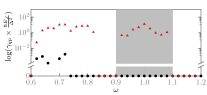
Figure 6: Quasi-particle creation rate $\gamma_{qp}$, computed for $N=20$ by replacing the $\delta$ function by a box of width $\delta E=0.02$, $t=-\Delta=\pi,\delta\mu=1,m_{max}=3$) for creating four quasi particles out of the vacuum using an adiabatically prepared Floquet system (red) and a system prepared by the frequency-sweep protocol of Fig. 4 (black). The grey shaded area shows the range where both Majorana zero modes and Majorana $\pi$ modes are available.

Appendix D Physical excitations and adiabatic continuity

In this section, we calculate analytically the Floquet-Bogoliubov spectrum in the bulk for small amplitudes of the oscillating potential. Our starting point is the static BCS Hamiltonian describing a single wire in the absence of the oscillating gate voltage.

$$H_{\text{BdG}}=\frac{1}{2}\sum_{k}(c^{\dagger}_{k},c_{-k})\left(\begin{array}[]{cc}-(\mu+t\cos k)&-i\Delta\sin k\\ i\Delta\sin k&\mu+t\cos k\\ \end{array}\right)\left(\begin{array}[]{c}c_{k}\\ c^{\dagger}_{-k}\end{array}\right)$$ (18)

Using a Bogoliubov transformation, we diagonalize the Hamiltonian

$$H_{BdG}=\frac{1}{2}\sum_{k}(a^{\dagger}_{k},a_{-k})\left(\begin{array}[]{cc}E_{k}&0\\ 0&-E_{k}\\ \end{array}\right)\left(\begin{array}[]{c}a_{k}\\ a^{\dagger}_{-k}\end{array}\right)=\sum_{k}E_{k}a^{\dagger}_{k}a_{k}$$ (19)

with $E_{k}=\sqrt{(\mu+t\cos k)^{2}+\Delta^{2}}$. The groundstate $|0\rangle$ is obtained from the condition $a_{k}|0\rangle=0$.

The oscillating gate voltage induces an oscillating potential $V(\tau)=\delta\mu\cos(\omega\tau)$ described by

$$H_{\text{drive}}(\tau)=-V(\tau)\sum_{k}c^{\dagger}_{k}c_{k}=\frac{1}{2}\sum_{k}\frac{V(\tau)}{E_{k}}\,(a^{\dagger}_{k},a_{-k})\left(\begin{array}[]{cc}-\mu-t\cos k&i\Delta\sin k\\ -i\Delta\sin k&\mu+t\cos k\\ \end{array}\right)\left(\begin{array}[]{c}a_{k}\\ a^{\dagger}_{-k}\end{array}\right).$$ (20)

Here we switch to the Floquet formalism [45]. In the Heisenberg picture, we make the following Floquet-Bogoliubov ansatz for new Floquet quasi-particle operators,

$$\tilde{a}_{k}^{\dagger}(\tau)=\sum_{n=-N}^{N}u_{k,n}\,e^{i(E_{k}^{\text{FL}}+n\omega)\tau}\,a_{k}^{\dagger}+v_{k,n}\,e^{-i(E_{k}^{\text{FL}}+n\omega)\tau}\,a_{-k}.$$ (21)

where $E_{k}^{\text{FL}}$ are the Floquet quasi-energies, defined modulo $\omega$. We choose the Floquet energies to be in the interval $0\leq E_{k}^{\text{FL}}<\omega$ and $N$ determines the number of Floquet modes. For an exact solution, one has to take the limit $N\to\infty$, but for small $\delta\mu$, the result converges rapidly even for small $N$. The $u_{k,n}$ and $v_{k,n}$ are determined from the condition (i) that the new operators obey the canonical anti-commutation relations of fermions and (ii) that $\tilde{a}_{k}^{\dagger}$ and $\tilde{a}_{-k}$ fulfill the Heisenberg equations of motion. This results in a matrix equation, $E_{k}^{\text{FL}}w^{\text{FL}}=H_{k}^{\text{FL}}w^{\text{FL}}$ where $H_{k}^{\text{FL}}$ is the (single-particle) Floquet Hamilitonian (or “Floquet matrix”) for fixed momentum $k$ and the vector $w^{\text{FL}}$ has the $2(2N+1)$ components $u_{k,n}$ and $v_{k,n}$, $-N\leq n\leq N$. Importantly, these conditions do not completely fix the quasi-particle operators as one can always perform a particle-hole transformation (not to be confused with a particle-hole symmetry operation [46])

$$\tilde{a}_{k}^{\dagger}\longleftrightarrow\tilde{a}_{-k},\qquad E_{k}^{\text{FL}}\longleftrightarrow-E_{k}^{\text{FL}}+\omega.$$ (22)

We added $+\omega$ in the last equation to ensure that the quasi-energy remains in the Floquet zone, $0\leq-E_{k}^{\text{FL}}+\omega<\omega$. In a more general setup where the $k\to-k$ symmetry is absent, one can, equivalently, consider the discrete transformation $\tilde{a}_{m}^{\dagger}\leftrightarrow\tilde{a}_{m}$ and $E_{m}^{\text{FL}}\longleftrightarrow-E_{m}^{\text{FL}}+\omega$ for Floquet-Bogoliubov states with quantum number $m$.

The ambiguity of Eq. (22) can be fixed by observing that the annihilation operators have to fulfill an extra condition: they should annihilate the adiabatically prepared initial state $|\psi_{0}\rangle$,

$$\tilde{a}_{k}|\psi_{0}\rangle=0.$$ (23)

Thus the preparation protocol of the state $|\psi_{0}\rangle$ is needed to identify correct annihilation and creation operators and to resolve the discrete ambiguity in the operators and quasi-energies expressed in Eq. (22). For any adiabatic preparation protocol there is a simple and unique way to identify the correct ground state and thus the correct quasi energies of excitations, $\tilde{a}_{k}|\psi_{0}\rangle$. The starting point is the groundstate of a static Hamiltonian, where all (physical) excitation energies are by definition positive. Then we can simply use the principle of adiabatic continuity to track the operators: a creation operator stays a creation operator during adiabatic evolution.

As we have shown in the main text, different adiabatic protocols (frequency sweep vs. amplitude sweep) with the same final $H(\tau)=H_{\text{BdG}}+H_{\text{drive}}(\tau)$ lead to different sets of creation and annihilation operators and thus different physical excitation energies.

We have done this adiabatic tagging of operators numerically for the system with open boundary conditions simply by tracking the evolution of excitation energies during the adiabatic evolution. Below, we give an analytically tractable example by considering weak oscillations, $\delta\mu\ll\omega,\Delta$, in an infinite system. In this case one can focus on approximately resonant processes with $E_{k}\approx-E_{k}+\omega$. Ignoring all non-resonant processes, the infinitely large Floquet matrix can be reduced to a simple $2\times 2$ matrix,

$$H^{\text{FL}}_{k}=\left(\begin{array}[]{cc}-E_{k}+\omega&\delta\mu\,f_{k}\\ \delta\mu\,f^{*}_{k}&E_{k}\\ \end{array}\right)$$ (24)

with $f_{k}=-i\frac{\Delta\sin k}{2\sqrt{(\mu+t\cos k)^{2}+\Delta^{2}\sin^{2}k}}$. The eigenvalues of this $2\times 2$ matrix are thus $\frac{\omega}{2}\pm\sqrt{\left(\delta\mu|f_{k}|\right)^{2}+\left(E_{k}-\omega/2\right)^{2}}$ where one of the energies is a physical excitation quasi-energy (multiplying $\tilde{a}_{k}^{\dagger}\tilde{a}_{k}$ in the second-quantized formula) while the other quasi-energy is the Bogoliubov shadow (multiplying $\tilde{a}_{k}\tilde{a}_{k}^{\dagger}$). Which one is which, depends on the protocol.

Let us consider the protocol where $\delta\mu$ is increased adiabatically at fixed frequency $\omega$. We track the energies back to $\delta\mu=0$ and demand that the physical excitation quasi-energy matches the physical excitation energy $E_{k}$ of the initial state

$$\lim_{\delta\mu\to 0}\frac{\omega}{2}\pm\sqrt{(\delta\mu|f_{k}|)^{2}+(E_{k}-\omega/2)^{2}}=\frac{\omega}{2}\pm|E_{k}-\omega/2|\stackrel{{\scriptstyle!}}{{=}}E_{k}.$$ (25)

Thus we should use the $+$ sign ($-$ sign) for $E_{k}>\omega/2$ ($E_{k}<\omega/2$). The physical excitation quasi-energies are then given by

$$E^{\text{FL}}_{k}=\left\{\begin{array}[]{ll}\frac{\omega}{2}+\sqrt{(\delta\mu|f_{k}|)^{2}+(E_{k}-\omega/2)^{2}}&\text{for }E_{k}>\omega/2\\[2.84526pt] \frac{\omega}{2}-\sqrt{(\delta\mu|f_{k}|)^{2}+(E_{k}-\omega/2)^{2}}&\text{for }E_{k}<\omega/2\end{array}\right..$$ (28)

There is therefore a jump in the excitation quasi-energy at $k=k_{0}$ where $E_{k_{0}}-\omega/2$ changes sign, see Fig. 3 of the main text.

Let us consider the“frequency-sweep” protocol, see Fig. 4 of the main text. Here one starts by increasing $\delta\mu$ using a small frequency where $E_{k}>\omega/2$ for all $k$. Thus, the physical excitation quasi-energy always has the $+$ sign in front of the square root. If one increases in a second step $\omega$ to reach the same final state as above, one always stays in the $+$ branch. Thus the physical excitation energies, in this case, are simply

$$E^{\text{FL}}_{k}=\frac{\omega}{2}+\sqrt{(\delta\mu|f_{k}|)^{2}+(E_{k}-\omega/2)^{2}}$$ (29)

for all momenta $k$. We would like to stress that the different excitation energies of the two protocols, Eqs. (28) and (29), arise because two very different many-particle wave functions are created in the two cases.

References

- Kitaev [2001] A. Y. Kitaev, Unpaired Majorana fermions in quantum wires, Phys. Usp. 44, 131 (2001), arXiv:cond-mat/0010440 .
- Ivanov [2001] D. A. Ivanov, Non-abelian statistics of half-quantum vortices in -wave superconductors, Phys. Rev. Lett. 86, 268 (2001).
- Read and Green [2000] N. Read and D. Green, Paired states of fermions in two dimensions with breaking of parity and time-reversal symmetries and the fractional quantum hall effect, Phys. Rev. B 61, 10267 (2000).
- Fu and Kane [2008] L. Fu and C. L. Kane, Superconducting Proximity Effect and Majorana Fermions at the Surface of a Topological Insulator, Physical Review Letters 100, 096407 (2008).
- Alicea [2010] J. Alicea, Majorana fermions in a tunable semiconductor device, Physical Review B 81, 125318 (2010).
- Oreg et al. [2010] Y. Oreg, G. Refael, and F. von Oppen, Helical Liquids and Majorana Bound States in Quantum Wires, Physical Review Letters 105, 177002 (2010).
- Lutchyn et al. [2010] R. M. Lutchyn, J. D. Sau, and S. Das Sarma, Majorana fermions and a topological phase transition in semiconductor-superconductor heterostructures, Phys. Rev. Lett. 105, 077001 (2010).
- Brouwer et al. [2011] P. W. Brouwer, M. Duckheim, A. Romito, and F. von Oppen, Topological superconducting phases in disordered quantum wires with strong spin-orbit coupling, Physical Review B 84, 144526 (2011).
- Manousakis et al. [2017] J. Manousakis, A. Altland, D. Bagrets, R. Egger, and Y. Ando, Majorana qubits in a topological insulator nanoribbon architecture, Physical Review B 95, 165424 (2017).
- Lutchyn et al. [2018] R. M. Lutchyn, E. P. A. M. Bakkers, L. P. Kouwenhoven, P. Krogstrup, C. M. Marcus, and Y. Oreg, Majorana zero modes in superconductor–semiconductor heterostructures, Nature Reviews Materials 3, 52 (2018).
- Flensberg et al. [2021] K. Flensberg, F. von Oppen, and A. Stern, Engineered platforms for topological superconductivity and Majorana zero modes, Nature Reviews Materials 10.1038/s41578-021-00336-6 (2021).
- Plugge et al. [2017] S. Plugge, A. Rasmussen, R. Egger, and K. Flensberg, Majorana box qubits, New Journal of Physics 19, 012001 (2017).
- Karzig et al. [2017] T. Karzig, C. Knapp, R. M. Lutchyn, P. Bonderson, M. B. Hastings, C. Nayak, J. Alicea, K. Flensberg, S. Plugge, Y. Oreg, C. M. Marcus, and M. H. Freedman, Scalable designs for quasiparticle-poisoning-protected topological quantum computation with majorana zero modes, Phys. Rev. B 95, 235305 (2017).
- Vijay and Fu [2016] S. Vijay and L. Fu, Teleportation-based quantum information processing with Majorana zero modes, Physical Review B 94, 235446 (2016).
- Kitagawa et al. [2010] T. Kitagawa, E. Berg, M. Rudner, and E. Demler, Topological characterization of periodically driven quantum systems, Phys. Rev. B 82, 235114 (2010).
- Wilczek [2012] F. Wilczek, Quantum time crystals, Phys. Rev. Lett. 109, 160401 (2012).
- Rudner et al. [2013] M. S. Rudner, N. H. Lindner, E. Berg, and M. Levin, Anomalous edge states and the bulk-edge correspondence for periodically driven two-dimensional systems, Phys. Rev. X 3, 031005 (2013).
- Nathan and Rudner [2015] F. Nathan and M. S. Rudner, Topological singularities and the general classification of floquet–bloch systems, New Journal of Physics 17, 125014 (2015).
- von Keyserlingk and Sondhi [2016] C. W. von Keyserlingk and S. L. Sondhi, Phase structure of one-dimensional interacting floquet systems. i. abelian symmetry-protected topological phases, Phys. Rev. B 93, 245145 (2016).
- Else and Nayak [2016] D. V. Else and C. Nayak, Classification of topological phases in periodically driven interacting systems, Phys. Rev. B 93, 201103(R) (2016).
- Else et al. [2016] D. V. Else, B. Bauer, and C. Nayak, Floquet time crystals, Phys. Rev. Lett. 117, 090402 (2016).
- Potter et al. [2016] A. C. Potter, T. Morimoto, and A. Vishwanath, Classification of interacting topological floquet phases in one dimension, Phys. Rev. X 6, 041001 (2016).
- Titum et al. [2016] P. Titum, E. Berg, M. S. Rudner, G. Refael, and N. H. Lindner, Anomalous floquet-anderson insulator as a nonadiabatic quantized charge pump, Phys. Rev. X 6, 021013 (2016).
- Roy and Harper [2016] R. Roy and F. Harper, Abelian floquet symmetry-protected topological phases in one dimension, Phys. Rev. B 94, 125105 (2016).
- von Keyserlingk et al. [2016] C. W. von Keyserlingk, V. Khemani, and S. L. Sondhi, Absolute stability and spatiotemporal long-range order in floquet systems, Phys. Rev. B 94, 085112 (2016).
- Jiang et al. [2011] L. Jiang, T. Kitagawa, J. Alicea, A. R. Akhmerov, D. Pekker, G. Refael, J. I. Cirac, E. Demler, M. D. Lukin, and P. Zoller, Majorana fermions in equilibrium and in driven cold-atom quantum wires, Phys. Rev. Lett. 106, 220402 (2011).
- Liu et al. [2012] D. E. Liu, A. Levchenko, and H. U. Baranger, Floquet Majorana Fermions for Topological Qubits, Phys. Rev. Lett. 111, 047002 (2013) (2012), arXiv:1211.1404 [cond-mat.mes-hall] .
- Kundu and Seradjeh [2013] A. Kundu and B. Seradjeh, Transport signatures of floquet majorana fermions in driven topological superconductors, Phys. Rev. Lett. 111, 136402 (2013).
- Li et al. [2014] Y. Li, A. Kundu, F. Zhong, and B. Seradjeh, Tunable floquet majorana fermions in driven coupled quantum dots, Phys. Rev. B 90, 121401(R) (2014).
- Liu et al. [2019] D. T. Liu, J. Shabani, and A. Mitra, Floquet majorana zero and modes in planar josephson junctions, Phys. Rev. B 99, 094303 (2019).
- Peng et al. [2021] C. Peng, A. Haim, T. Karzig, Y. Peng, and G. Refael, Floquet majorana bound states in voltage-biased planar josephson junctions, Phys. Rev. Research 3, 023108 (2021).
- Peng and Refael [2018] Y. Peng and G. Refael, Time-quasiperiodic topological superconductors with majorana multiplexing, Physical Review B 98, 220509(R) (2018).
- Bauer et al. [2019] B. Bauer, T. Pereg-Barnea, T. Karzig, M.-T. Rieder, G. Refael, E. Berg, and Y. Oreg, Topologically protected braiding in a single wire using floquet majorana modes, Phys. Rev. B 100, 041102(R) (2019).
- Bomantara and Gong [2020] R. W. Bomantara and J. Gong, Measurement-only quantum computation with floquet majorana corner modes, Phys. Rev. B 101, 085401 (2020).
- Jens Koch and Terri M. Yu and Jay Gambetta and A. A. Houck and D. I. Schuster and J. Majer and Alexandre Blais and M. H. Devoret and S. M. Girvin and R. J. Schoelkopf [2007] Jens Koch and Terri M. Yu and Jay Gambetta and A. A. Houck and D. I. Schuster and J. Majer and Alexandre Blais and M. H. Devoret and S. M. Girvin and R. J. Schoelkopf, Charge-insensitive qubit design derived from the cooper pair box, Physical Review A 76, 042319 (2007).
- Polkovnikov [2005] A. Polkovnikov, Universal adiabatic dynamics in the vicinity of a quantum critical point, Physical Review B 72, 161201(R) (2005).
- Zurek et al. [2005] W. H. Zurek, U. Dorner, and P. Zoller, Dynamics of a quantum phase transition, Physical Review Letters 95, 105701 (2005).
- Damski [2005] B. Damski, The simplest quantum model supporting the kibble-zurek mechanism of topological defect production: Landau-zener transitions from a new perspective, Physical Review Letters 95, 035701 (2005).
- Dziarmaga [2005] J. Dziarmaga, Dynamics of a quantum phase transition: Exact solution of the quantum ising model, Physical Review Letters 95, 245701 (2005).
- Landau [1932] L. Landau, On the theory of transfer of energy at collisions ii, Phys. Z. Sowjetunion 2, 118 (1932).
- Zener [1932] C. Zener, Non-adiabatic crossing of energy levels, Proceedings of the Royal Society of London. Series A, Containing Papers of a Mathematical and Physical Character 137, 696 (1932).
- Seetharam et al. [2015] K. I. Seetharam, C.-E. Bardyn, N. H. Lindner, M. S. Rudner, and G. Refael, Controlled Population of Floquet-Bloch States via Coupling to Bose and Fermi Baths, Phys. Rev. X 5, 041050 (2015).
- Bilitewski and Cooper [2015] T. Bilitewski and N. R. Cooper, Scattering theory for Floquet-Bloch states, Phys. Rev. A 91, 033601 (2015).
- Genske and Rosch [2015] M. Genske and A. Rosch, Floquet-Boltzmann equation for periodically driven Fermi systems, Phys. Rev. A 92, 062108 (2015).
- Rudner and Lindner [2020] M. S. Rudner and N. H. Lindner, The Floquet Engineer’s Handbook, arXiv preprint arXiv:2003.08252 (2020), arXiv:2003.08252 [cond-mat.mes-hall] .
- Zirnbauer [2021] M. R. Zirnbauer, Particle–hole symmetries in condensed matter, Journal of Mathematical Physics 62, 021101 (2021), https://doi.org/10.1063/5.0035358 .