Lattice Simulation of Multi-Stream Inflation

Abstract

We present the first lattice simulation to investigate the nature of multi-stream inflation. The simulation confirms the physical picture of multi-stream inflation, and with new findings in parameter space and field behaviors. Our simulation shows that gradient energy plays a significant role in multi-stream inflation. For a double field potential with a shifted Gaussian barrier, bifurcation probability is controlled by the shift distance with an error function relation. The bubbles created by bifurcation tend to be more spherical as bifurcation probability decreases. Also, the bifurcation is more likely to introduce oscillations of field values inside the bubbles than outside.

I introduction

Inflation has been the leading paradigm of the early universe Guth (1981); Linde (1982); Starobinsky (1980); Brout et al. (1978); Sato (1981); Fang (1980); Albrecht and Steinhardt (1982) to solve several conundrums of the Hot Big Bang, and provide origin of the density fluctuations which serve as the seeds of large scale structure.

Motivated by the string landscape Bousso and Polchinski (2000); Susskind (2003), the inflationary dynamics may be not as simple as the prototype. As illustrated in Fig. 1, in the multi-field space, if the inflationary trajectory encounters a barrier, bifurcation of the inflationary trajectory can happen. The local universes may undergo inflation along either A or B trajectories as marked in the figure. This bifurcation behavior is known as multi-stream inflation Li and Wang (2009). Bifurcation behavior in a random potential is spotted in Duplessis et al. (2012) and increasing the dimension of the random field space can increase the probability of bifurcations Liu et al. (2015).

The observational consequences of multi-stream inflation include: (i) Due to the $\delta N$ formalism Starobinsky (1985); Sasaki and Stewart (1996); Lyth and Rodriguez (2005), the e-folding number difference between multiple trajectories is an additional source of curvature perturbation at the bifurcation scale Li and Wang (2009). Depending on the scale of bifurcation, this additional perturbation may be responsible for features on the CMB, the CMB cold spot Afshordi et al. (2011), or primordial black hole formation Nakama et al. (2016) when the comoving scale corresponding to the bifurcation returns to the horizon. (ii) The local environments along different inflationary trajectories (A and B in Fig. 1) can be different. The difference can be responsible for position space anomalies of the universe, such as power asymmetries on the CMB Li and Wang (2009); Wang (2013), clustered production of primordial black holes Ding et al. (2019) and stellar bubbles Cai et al. (2021). And correlation between the bifurcation scale and the local environments introduce non-Gaussianities Li and Wang (2009); Abolhasani et al. (2011). (iii) The domain wall in between A and B can have observational effects Li et al. (2009), and the thickness of the domain wall can help evade the Sunyaev-Zeldovich effect constraints when using voids to ease the Hubble tension problem Ding et al. (2020). If the bifurcated trajectories finally combine (or merge to connected degenerate vacuum configurations in the case of multiple isocurvature directions), the tension of the domain wall finally vanish and thus it does not cause the conventional domain wall problem in cosmology.

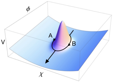
Figure 1: Multi-stream inflation: how the bifurcation in the isocurvature direction during inflation generate bubbles, inflaton for most part of the universe follows trajectory A while some follow trajectory B.

Although many observational features in multi-stream inflation can be estimated by the separate universe picture and the $\delta N$ formalism, quantitative analytical calculation is usually difficult in multi-stream inflation. This is because of the temporary domain wall in between the two trajectories. The domain wall is dynamical and introduces additional gradient energy to the field configuration. Although the observational consequences of the domain wall is discussed in the literature Li et al. (2009); Ding et al. (2020), how the domain wall affects the bifurcation dynamics was not studied. Also, the previous numerical simulations of the bifurcation probability were built upon the $\delta N$ formalism which did not take the domain wall and gradient energy into account Duplessis et al. (2012); Liu et al. (2015). Statobinsky’s stochastic approach was used to study the dynamics of bifurcation Liu et al. (2015). The difference between its analysis of bifurcation and that of lattice codes is that stochastic approach can only show the fluctuations away from the domain wall, but not the ones close to it due to the strong gradient and potential energy. Since the interplay between the domain wall and the nearby bifurcated field is nonlinear, and inhomogeneous in space, we expect that the effect has to be simulated by lattice simulation. Also, the bifurcation may introduce oscillations, which is also strongly affected by the gradient energy.

In the literature of the very early universe cosmology, lattice codes are widely used in simulating reheating after inflation. During inflation, simulations are possible (see, for example, Caravano et al. (2021)) but the computation is challenging because of the exponential expansion of the space volume. In our case, we will by-pass this difficulty by studying only a few e-folds of inflation around the bifurcation time. This suffices the study of the dynamics of the domain wall and how it affects the bifurcation. In this paper, we use a modified version of LATTICEEASY Felder and Tkachev (2008) to simulate the multi-stream inflation.

This paper is organized as follows. Sec. II provides the basic equations for the dynamics of inflation. Then we take a potential of multi-stream inflation, and simulate bifurcations in Sec. III. We discuss the effects of gradient energy, then investigate some important features of multi-stream inflation, including bifurcation probability, potential shift, bubble sphericity as well as oscillatory behaviors of trajectories corresponding to the bubble region. We conclude in Sec. IV. Some details about the calculation of background potential and bubble sphericity are presented in Appendix A and B.

We will work in Planck units, with $c=\hbar=G=1$ and the reduced Planck mass $M_{p}=1/\sqrt{8\pi}$. Dot is used to denote derivative with respect to cosmic time ($\dot{\ }=d/dt$).

II Evolution Equations

We study the dynamics of scalar fields, ignoring the backreaction by gravity. We start from the Friedmann-Lemaître-Robertson-Walker (FLRW) metric:

$$ds^{2}=-dt^{2}+a^{2}(t)(dx^{2}+dy^{2}+dz^{2}),$$ (1)

where $a$ is the scale factor. And the Friedmann equations for background evolution are:

$$3H^{2}=8\pi\rho,\ \ \frac{\ddot{a}}{a}=-\frac{4\pi}{3}(\rho+3p),$$ (2)

where $H\equiv\dot{a}/a$ is the Hubble parameter describing the expansion rate of the universe. The energy density $\rho$ and pressure $p$ for scalar fields are

$$\rho=T+G+V,\ \ p=T-\frac{1}{3}G-V,$$ (3)

with kinetic energy $T$ and gradient energy $G$:

$$T=\frac{1}{2}\dot{\phi}^{2}+\frac{1}{2}\dot{\chi}^{2},\ \ G=\frac{1}{2a^{2}}|\nabla\phi|^{2}+\frac{1}{2a^{2}}|\nabla\chi|^{2}.$$ (4)

The equations of motion for the scalar fields are

$$\begin{split}\ddot{\phi}+3H\dot{\phi}-\frac{\nabla^{2}}{a^{2}}\phi+\frac{\partial V}{\partial\phi}=0,\\ \ddot{\chi}+3H\dot{\chi}-\frac{\nabla^{2}}{a^{2}}\chi+\frac{\partial V}{\partial\chi}=0.\end{split}$$ (5)

Different from LATTICEEASY, we here uses Runge-Kutta methods to numerically solve these classical equations. We focus on the evolution of such inhomogeneous background fields in our parameter space. As for the quantum nature of the inflaton, it is described by the statistical uncertainty generated by semi-classical approximation Felder and Tkachev (2008); Caravano et al. (2021). That is to say the methods we use to determine initial conditions are the same as LATTICEEASY.

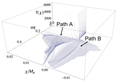
Figure 2: Simulated inflaton trajectories in the potential with a barrier. $f(\chi)$ represents probability density of $\chi$ at different time. Trajectory A rolls on one side of the barrier and B rolls on the other side of it after bifurcation and before combination of these trajectories.

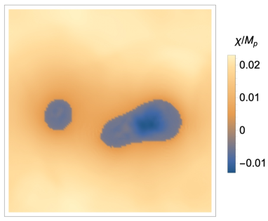
Figure 3: Two-dimensional slice of the lattice points during the bifurcation, we can see the cross-sections of the bubbles created, which are the blue parts.

III Toy Model with a barrier

We consider a potential with a barrier, around which multi-stream inflation takes place:

$$\begin{split}V(\phi,\chi&)=\frac{1}{2}m^{2}\phi^{2}+\frac{1}{2}\alpha m^{2}\chi^{2}+\\ &\beta m^{2}\text{e}^{-[\frac{(\phi-\phi_{b})^{2}}{2\sigma_{1}^{2}}+\frac{(\chi-\chi_{b})^{2}}{2\sigma_{2}^{2}}]},\end{split}$$ (6)

where $\beta$ is a constant controlling the height of the barrier. The parameters $\phi_{b},\chi_{b}$ decides barrier position and $\phi_{0}=16M_{p},\chi_{0}=0$ are the initial values of fields.

As shown in Fig. 1 and Fig. 3 the inflaton rolls down this potential, its trajectories bifurcate after hitting the barrier, creating bubbles in the universe. We then focus on some phenomena concerning such bifurcation. Fig. 2 is a series of plots of trajectory $\chi$ distributions, where we can easily see the whole process of bifurcation.

III.1 Gradient Energy

In this subsection we show the effect of gradient energy, and how it affects the dynamics of bifurcation. If we set the potential of the barrier to be a bit shifted from the center of the background potential, that is to set $0<\chi_{b}\ll 1$ in Eq. 6, then we have an asymmetric bifurcation as an example condition for simulation.

In this simulation above, the distribution of trajectories is shown as Fig. 4. While a small number of trajectories roll below the potential barrier, most of them roll above the barrier, these two kinds of trajectories correspond to trajectory B and A in Fig. 2 respectively.

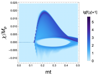
Figure 4: $\chi$ value distribution of trajectories in different time, gradient energy is included in the simulation as it should be. $f(\chi)$ is the probability distribution.

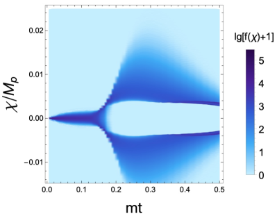
Figure 5: $\chi$ value distribution of trajectories in different time with gradient energy being set to zero. $f(\chi)$ is the probability density of distribution.

We can immediately realize that although there are both bifurcations happening in Fig. 2 and Fig. 4, there are obvious differences in the shape of trajectories. In Fig. 2 we assume the trajectories would stay close to the barrier just as the black curves show. However, in Fig. 4 where the actual trajectories are shown, it turns out that most of the trajectories roll away from the barrier before coming back due to the $\alpha m^{2}\chi^{2}/2$ term. Does gradient energy contribute to such behavior? In order to find out we run the simulation again using all the same conditions but setting the gradient energy to zero. The result of such simulation is shown as Fig. 5. Without gradient energy, the lattice points in the simulation box are independent of each other and the shapes of trajectories are fully determined by the potential, leading to the fact that before bifurcation the distribution in Fig. 5 is wider and more symmetric than that in Fig. 4. As the distributions have many differences with or without gradient energy, it surely has critical effect on the bifurcation itself. That is to say, gradient energy does contribute to the behavior of trajectories in a complicated way. It is hard to evaluate such effect analytically, so numerical simulation might be a more appropriate way.

The effects of gradient energy here is complicated, we cannot simply claim that its existence always help making the trajectories move away from the barrier, instead this is only confirmed in the parameter space that we choose. For example, what if the barrier in the potential is much larger, will the trajectories move closer from the barrier? We are unable to answer this question at the moment because the number of e-folds that lattice simulation can run is limited.

As we discuss above, the $\chi$ distribution of trajectories is wider when the potential energy is gone before bifurcation, that is because although initial value fluctuation of $\chi$ is relatively small at $(mt,\chi/M_{p})=(0,0)$, trajectories will immediately move towards different directions and apart from each other since they have different initial field derivatives $\dot{\chi}$.

Another issue is the bifurcation probability. In Fig. 4 and Fig. 5, apart from the gradient energy, we have exactly identical initial conditions and potential barrier position $\phi_{b},\chi_{b}$, yet the simulation shows that in Fig. 5 the bifurcation is nearly symmetric, while in Fig. 4, asymmetry is significant and only a small fraction of trajectories take path B (downwards) instead of path A (upwards). Clearly it is the existence of gradient energy that cause the significant asymmetry. Gradient energy creates a strong bound among the trajectories. That is to say the trajectories tend to move as a group facing a bifurcation, this is confirmed by Fig. 4 since we can see that trajectory distribution has been narrow.

As gradient energy was not considered when $\delta N$ formalism was used to estimate some features in previous works, the results were not enough to recover many of the details during bifurcation. This is no longer a problem in this paper since lattice simulation can take gradient energy into account.

III.2 Bifurcation Probability and Potential Shift

The bifurcation probability is influenced by the position of the barrier, if the barrier center is at the bottom of potential $\alpha m^{2}\chi^{2}/2$ term. In other words, if $\chi_{b}=\chi_{0}=0$ in Eq. 6, then the bifurcation is almost symmetric. When moving away from this symmetric point, the bifurcation probability becomes asymmetric.

In the separate universe picture, we expect that the bifurcation probability is an error function as a function of $\chi_{b}$. This is because the bifurcation is controlled by the fluctuation of $\chi$ exceeding a threshold, which follows an approximately Gaussian distribution.

Considering the effect of gradient energy, the relation between the bifurcation probability and $\chi_{b}$ is less obvious. Because the gradient energy affects the bifurcation probability significantly. Nevertheless, our simulation result show that this relation still takes the form of an error function.

Fig. 6 shows that for different random seeds, which means for different initial fluctuations, bifurcation probability increases smoothly as the potential barrier moves in $\chi$ direction. As displayed in Fig. 7, this function can be well fitted by the error function

$$\text{P}_{\text{bif}}=\frac{1}{2}+\frac{1}{2}\text{erf}(\frac{\delta}{\sqrt{2}\sigma}),$$ (7)

where $\delta=\chi_{b}/M_{p}$ is the rescaled potential shift distance.

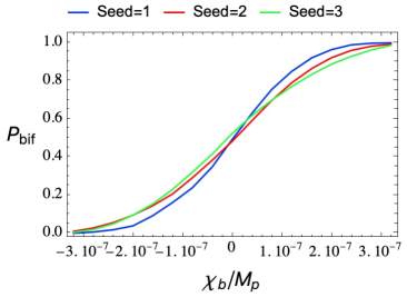
Figure 6: Simulation results of bifurcation probability as a function of shift distance, different colors represent different initial random seed. Randomness of initial fluctuation might cause small changes in the curves, but it does not change the fact that each curve is very close to error function curve.

Figure 7: One example of simulation results and fitted curve, blue dots are the simulation outputs, yellow curve is the fitted function.

It is natural to try to estimate the bifurcation probability by dividing gaussian distributions of $\chi$ field using position of barrier center $\chi_{b}$. While this indeed can lead to an error function relation, the parameter $\sigma$ of such function is significantly larger than the one obtained from simulation. The reason of it has been discussed in Sec. III.1. As gradient energy tend to connect different trajectories, a slight shift of the barrier position can cause the trajectory distribution to move as a whole, consequently reducing the value of $\sigma$ in Eq. 7

III.3 Bubble Sphericity and Bifurcation Probability

In lattice simulation we can extract bubbles and analyze their shapes. For very small bifurcation probability $\text{P}_{\text{bif}}\ll 1$, the shapes of bubbles are expected to be spherical Afshordi et al. (2011), following the peak theory Bardeen et al. (1986) (which will then be affected by the gradient energy of the field at the scale of the bifurcation), or alternatively considered as instantons in quantum field theory minimizing the Euclidean action Coleman (1977). It is thus theoretically expected for a bubble that the smaller $\text{P}_{\text{bif}}$, the more spherical.

However, if we are not talking about exponentially small $\text{P}_{\text{bif}}$, for small but still significant $\text{P}_{\text{bif}}$, the trend of sphericity is less clear. In this subsection, we test the sphericity as a function of $\text{P}_{\text{bif}}$. We confirm the trend of more spherical bubbles for a smaller bifurcation probability, but also show that the result has large variance, and the initial condition also affects the sphericity significantly. To eliminate the impact from the initial condition, we choose to focus on a certain simulation setup with fixed initial condition, while changing bifurcation probability by shifting the position of the barrier, to track how it changes sphericity.

To measure how spherical a bubble is, limited by the resolution of the lattice, we compare the bubble with a spherical bubble with the same volume, and calculate their overlapping ratio. In this definition a perfectly spherical bubble has sphericity equals to 1. We tested that this definition is robust for a calculation on the lattice. The details and benchmarks of the definition of sphericity is provided in Appendix B.

Fig. 8 reveals that for different bubbles, although their sphericity curves have can be quite different, these curves all show that sphericity tends to be smaller as bifurcation probability increases. Here we have chosen the parameter space for intermediate bifurcation probability, to have enough samples of bubbles with clear bubble identification.

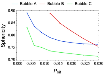
Figure 8: Sphericity as a function of bifurcation probability, different color represents different bubble.

III.4 Oscillation of the Individual Trajectories

In Fig. 4, we have plotted the $\chi$ value distributions. In Fig. 9, we investigate the dynamics of the bifurcation in more details to plot individual trajectories. It is interesting to note that oscillations generically arise in the trajectories with smaller probability, but is absent for the trajectory with larger probability. In position space, this corresponds to oscillations of field values in bubbles, but not outside bubbles.

This effect can be understood as in the more probable trajectory, the kinetic energy drives the trajectory to very large $\chi$ value in a short time, away from the potential minima. This is known as a “feature scattering” Wang and Ma (2016). There is thus lack of oscillation since the field is not around the minima. Then, the dynamics is smoother, and the Hubble fraction damps the kinetic energy.

In the literature, there have been extensive studies on the oscillations and how to extract the information of inflation from these oscillations. For example, these oscillations can behave as primordial standard clocks Chen (2012); Chen et al. (2015) to measure the evolution history of the primordial universe. Our simulation points to an interesting possibility of having primordial standard clock signals in bubbles (such as a void in the large scale structure), but not outside. The oscillations may also bring additional non-Gaussian signatures similar to that of Sugimura et al. (2012).

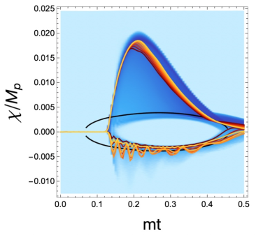
Figure 9: Samples of trajectories following the two different paths. Here the black curve is the local minima of the potential. Note that the lower trajectories with smaller probability of bifurcation in general have more significant oscillations.

This oscillatory behavior of the trajectories also shed light on the dynamics of teh temporary domain walls in multi-stream inflation. Temporary domain walls correspond to the part of position space volume between different preferred trajectories. The dynamics of the domain wall region is interesting. For example, in Ding et al. (2020), it is noted that after combination of different inflationary trajectories, the domain wall tension vanishes and the domain wall region starts to expand with the exponential expansion of the universe. This can lead to a broad and smooth intermediate region between the void and outside, which is observationally less constraining from the Sunyaev-Zeldovich effect.

Since the trajectory is oscillating, the temporary domain wall has a time-dependent tension. Since domain walls can leave signatures in density fluctuations Jazayeri et al. (2014), even if their tension disappears later, it is interesting to explore the observational effects of the oscillatory tension of the domain wall. We hope we can address these issues in a future work.

IV Conclusion

In this paper we explore some features of multi-stream inflation using lattice simulation. We study a two-field potential with a barrier and find that the trajectories of multi-stream inflation greatly depend on gradient energy. We then analyze in detail how gradient energy play such an important role in the process of bifurcation by comparing the trajectory distribution with or without gradient energy. By comparison we show that gradient energy significantly contributes to the behavior of trajectory distribution. Next, we focus on how the position of this barrier influences bifurcation probability. It turns out that there is a clear error function relation between them. This error function relation cannot be explained simply by initial Gaussian fluctuation, instead it is also related to gradient energy. We also calculate bubble sphericity for different bifurcation probability, confirming that for rare peaks, bubbles tend to be more spherical. Finally, we note that in the less probable trajectories oscillation can take place, corresponding to oscillatory behaviors of observables in bubbles and domain walls, but not outside bubbles.

With the setup of the lattice code, many other aspects of multi-stream inflation may be studied, such as the details of the curvature power spectrum (which was only estimated by the $\delta N$ formalism), the dynamics of the domain walls and possible impacts with a random potential instead of a simple barrier. We hope to return to some of these topics in future studies.

Appendix A Background Potential
without a barrier

Before simulating multi-stream inflation in a potential with a barrier, we analyze our potential without a barrier, for conventional inflation dynamics without bifurcation. We use a quadratic double field potential to be our background potential

$$V(\phi,\chi)=\frac{1}{2}m^{2}\phi^{2}+\frac{1}{2}\alpha m^{2}\chi^{2},$$ (8)

where $m$ is the inflaton mass, $\alpha$ is the $\chi$ term parameter. $\phi_{0}=16M_{p},\chi_{0}=0$ are the initial values of fields.

For such a simple potential, it is clear that the inflation will proceed very close to single field inflation $V(\phi)=m^{2}\phi^{2}/2$. By simulating such a model, we can primarily confirm the validity of our simulation by comparing it with theoretical predictions, what is more important is that it represents the general behavior of our potentials.

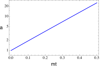
Figure 10: Evolution of scale factor.

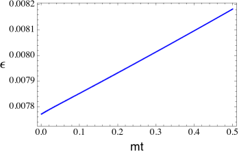
Figure 11: Evolution of slow-roll parameter $\epsilon$.

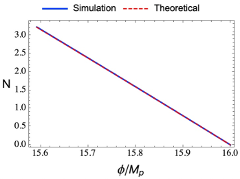
Figure 12: Number of e-folds as a function of $\phi/M_{p}$, blue curve is simulation result, yellow dashed curve is theoretical result, they match well.

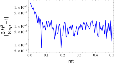
Figure 13: Fractional energy noise as a function of $mt$. It keeps increasing and reach the level of $10^{-7}$.

Fig. 10 $\sim$ 13 demonstrates some background values during inflation. We can tell that an slow-roll inflation is achieved from the evolution of scale factor and slow-roll parameter. Number of e-folds and value of $\phi$ are also plotted, the blue curve is simulation output while the yellow dashed curve is theoretical prediction, these two curves perfectly match.

To verify conservation of energy, we pay attention to the fractional energy noise $3H^{2}/(8\pi\rho)-1$ during inflation. In our case this quantity is roughly $10^{-7}$ and it tells that the computation is solid.

It is worth mentioning that when $0<mt<0.1$, the value of $|3H^{2}/(8\pi\rho)-1|$ is generally decreasing. The reason for it is that gradient energy is not taken into account during initialization, causing such anomaly at the beginning of simulation, yet such level of it is unimportant and barely affects our result.

These background values in Fig. 10 $\sim$ 13 represent a background inflation, that is to say when we add a barrier to the potential and change related parameters, the curves in are only slightly changed, approximately following the behaviors under a standard inflation. This is confirmed by actual simulation.

Appendix B Sphericity of Lattice Bubble

In Sec. III.3 we extract bubbles from the lattice and calculate sphericity. Here the challenge is to define sphericity on a lattice simulation. Since we have limited lattice resolution, we need the definition to be robust with relatively low lattice resolution. For this purpose, we define the sphericity as follows.

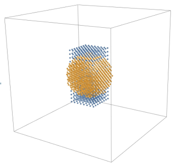
Figure 14: Calculation of sphericity. We want to calculate the sphericity of the object with blue points. Sphere with yellow points is the reference sphere that we take. Sphericity is then the ratio of number of mutual points that object and reference sphere share to number of points of object.

For an object consisting of $N_{t}$ lattice points, we average all the points separately for three coordinate directions to obtain the center point of this object, then we search the lattice points and select $N_{t}$ points closest to the center point to form a reference sphere. We define $N_{m}$ as the number of mutual points that object and reference sphere share, then

$$\text{Sphericity}=\frac{N_{m}}{N_{t}}.$$ (9)

Fig. 14 is an example of such sphericity calculation.

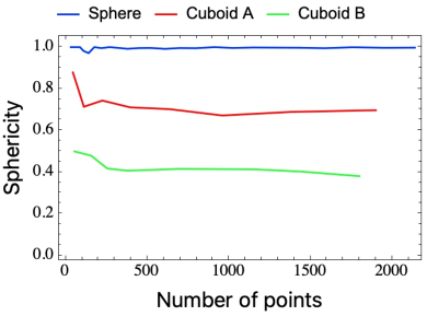
Figure 15: Sphericity as a function of number of points of the calculated object. Different colors represent different shapes of objects.

In Fig. 15 we calculate the sphericity of objects consisting of different number of lattice points. It turns out that for different objects the sphericity is stable. We set 300 as an threshold, that is to say we only take into account the sphericity of objects consisting of more than 300 lattice points. Our results in III.3 shows obvious tendency of sphericity, that is another confirmation of validity of this definition of sphericity.

References

- Guth (1981) A. H. Guth, Phys. Rev. D 23, 347 (1981).
- Linde (1982) A. D. Linde, Phys. Lett. B 108, 389 (1982).
- Starobinsky (1980) A. A. Starobinsky, Phys. Lett. B 91, 99 (1980).
- Brout et al. (1978) R. Brout, F. Englert, and E. Gunzig, Annals Phys. 115, 78 (1978).
- Sato (1981) K. Sato, Mon. Not. Roy. Astron. Soc. 195, 467 (1981).
- Fang (1980) L. Z. Fang, Phys. Lett. B 95, 154 (1980).
- Albrecht and Steinhardt (1982) A. Albrecht and P. J. Steinhardt, Phys. Rev. Lett. 48, 1220 (1982).
- Bousso and Polchinski (2000) R. Bousso and J. Polchinski, JHEP 06, 006 (2000), arXiv:hep-th/0004134 .
- Susskind (2003) L. Susskind, , 247 (2003), arXiv:hep-th/0302219 .
- Li and Wang (2009) M. Li and Y. Wang, JCAP 07, 033 (2009), arXiv:0903.2123 [hep-th] .
- Duplessis et al. (2012) F. Duplessis, Y. Wang, and R. Brandenberger, JCAP 04, 012 (2012), arXiv:1201.0029 [hep-th] .
- Liu et al. (2015) J. Liu, Y. Wang, and S. Zhou, Phys. Rev. D 91, 103525 (2015), arXiv:1501.06785 [hep-th] .
- Starobinsky (1985) A. A. Starobinsky, JETP Lett. 42, 152 (1985).
- Sasaki and Stewart (1996) M. Sasaki and E. D. Stewart, Prog. Theor. Phys. 95, 71 (1996), arXiv:astro-ph/9507001 .
- Lyth and Rodriguez (2005) D. H. Lyth and Y. Rodriguez, Phys. Rev. Lett. 95, 121302 (2005), arXiv:astro-ph/0504045 .
- Afshordi et al. (2011) N. Afshordi, A. Slosar, and Y. Wang, JCAP 01, 019 (2011), arXiv:1006.5021 [astro-ph.CO] .
- Nakama et al. (2016) T. Nakama, T. Suyama, and J. Yokoyama, Phys. Rev. D 94, 103522 (2016), arXiv:1609.02245 [gr-qc] .
- Wang (2013) Y. Wang, JCAP 10, 006 (2013), arXiv:1304.0599 [astro-ph.CO] .
- Ding et al. (2019) Q. Ding, T. Nakama, J. Silk, and Y. Wang, Phys. Rev. D 100, 103003 (2019), arXiv:1903.07337 [astro-ph.CO] .
- Cai et al. (2021) Y.-F. Cai, C. Chen, Q. Ding, and Y. Wang, (2021), arXiv:2105.11481 [astro-ph.CO] .
- Abolhasani et al. (2011) A. A. Abolhasani, H. Firouzjahi, and M. H. Namjoo, Class. Quant. Grav. 28, 075009 (2011), arXiv:1010.6292 [astro-ph.CO] .
- Li et al. (2009) S. Li, Y. Liu, and Y.-S. Piao, Phys. Rev. D 80, 123535 (2009), arXiv:0906.3608 [hep-th] .
- Ding et al. (2020) Q. Ding, T. Nakama, and Y. Wang, Sci. China Phys. Mech. Astron. 63, 290403 (2020), arXiv:1912.12600 [astro-ph.CO] .
- Caravano et al. (2021) A. Caravano, E. Komatsu, K. D. Lozanov, and J. Weller, (2021), arXiv:2102.06378 [astro-ph.CO] .
- Felder and Tkachev (2008) G. N. Felder and I. Tkachev, Comput. Phys. Commun. 178, 929 (2008), arXiv:hep-ph/0011159 .
- Bardeen et al. (1986) J. M. Bardeen, J. R. Bond, N. Kaiser, and A. S. Szalay, Astrophys. J. 304, 15 (1986).
- Coleman (1977) S. R. Coleman, Phys. Rev. D 15, 2929 (1977), [Erratum: Phys.Rev.D 16, 1248 (1977)].
- Wang and Ma (2016) Y. Wang and Y.-Z. Ma, Nucl. Phys. B 906, 367 (2016), arXiv:1501.00282 [astro-ph.CO] .
- Chen (2012) X. Chen, JCAP 01, 038 (2012), arXiv:1104.1323 [hep-th] .
- Chen et al. (2015) X. Chen, M. H. Namjoo, and Y. Wang, JCAP 02, 027 (2015), arXiv:1411.2349 [astro-ph.CO] .
- Sugimura et al. (2012) K. Sugimura, D. Yamauchi, and M. Sasaki, EPL 100, 29004 (2012), arXiv:1208.3937 [astro-ph.CO] .
- Jazayeri et al. (2014) S. Jazayeri, Y. Akrami, H. Firouzjahi, A. R. Solomon, and Y. Wang, JCAP 11, 044 (2014), arXiv:1408.3057 [astro-ph.CO] .