Abstract

The aim of this study is to search for quasi-periodical structures at moderate cosmological redshifts $z\;\raise 1.29167pt\hbox{$<$\kern-7.5pt\raise-4.73611pt\hbox{$\sim$}}\;0.5$. We mainly use the SDSS DR7 data on the luminous red galaxies (LRGs) with redshifts $0.16\leq z\leq 0.47$. At first, we analyze features (peaks) in the power spectra of radial (shell-like) distributions using separate angular sectors in the sky and calculate the power spectra within each sector. As a result, we found some signs of a large-scale anisotropic quasi-periodic structure detectable through 6 sectors out of a total of 144 sectors. These sectors are distinguished by large amplitudes of dominant peaks in their radial power spectra at wavenumbers $k$ within a narrow interval of $0.05<k<0.07$ h Mpc^-1. Then, passing from a spherical coordinate system to a Cartesian one, we found a special direction such that the total distribution of LRG projections on it contains a significant ( $>$$\sim$ 5$\sigma$) quasi-periodical component. We assume that we are dealing with a signature of a quasi-regular structure with a characteristic scale $116\pm 10$ h^-1 Mpc. Our assumption is confirmed by a preliminary analysis of the SDSS DR12 data.

statistical methods; distances and redshifts of galaxies; large-scale structure of Universe

1 Introduction

The large-scale distribution of the matter (dark and baryonic substances) in the Universe represents a very complex multi-scale structure (known as cosmic web, [1]) whose origin, evolution, dynamics and structural features have been the subject of extensive study for a few decades (e.g., [2]). The structure represents a network of high-density regions formed by galaxy clusters and superclusters, walls and filaments, delineating low-density regions $-$ giant voids, occupying the bulk of the space in the Universe (for review see, e.g. [3-5]).

The complex pattern of the cosmic web includes a huge variety of scales, ranging from units and tens of megaparsecs up to hundreds of megaparsecs. In this regard, it seems important to question the highlighted scales of inhomogeneities that appear in the largest observable structures and the related question of the possible existence of some geometric order, at least in certain parts of the cosmic web. Among the largest scales, the most frequently mentioned scales in the literature are $\;\raise 1.29167pt\hbox{$>$\kern-7.5pt\raise-4.73611pt\hbox{$\sim$}}\;100h^{-1}$ Mpc, where $h=H_{0}/100$ km s^-1 Mpc^-1 and $H_{0}$ is the present Hubble constant. These are, for instance, the characteristic scales of large voids $\sim 100\leavevmode\nobreak\ h^{-1}$ Mpc, the spatial scales (100–110) $h^{-1}$ Mpc corresponding to the Baryon Acoustic Oscillations (BAO, e.g., [6-8] and references therein), as well as somewhat larger scales found in ordered quasi-periodic formations. It is well known that the scale of the BAO is determined by the size of the horizon of sound waves in the recombination epoch and manifests itself as the presence of a weak periodic component in the 3D power spectrum of cosmological inhomogeneities (e.g., [9-11]). As a consequence of such oscillations in k-space, a significant bump is registered in the spatial 3D correlation function at the scales noted above (e.g., [12-16] and references therein).

On the other hand, we have a number of observational evidence that some areas of the cosmic web show elements of spatial regularity at scales of the order of (110–140) $h^{-1}$ Mpc. Important evidence of the existence of some order in the spatial distribution of galaxies was the detection of 1D quasi-periodicity at a scale $\sim$130 $h^{-1}$ Mpc found in the pencil-beam surveys near both Galactic poles [17]. This result was confirmed (but see note in Section 6) in further studies of pencil-beam distributions of galaxies [18-20]. This was followed by a series of works, e.g.,  [21-26], in which it was shown that the cosmological network formed by rich clusters and superclusters of galaxies and voids between them may show traces of a regular spatial (cubic-like or shell-like) structure, with characteristic scales (110–140) $h^{-1}$ Mpc.

Using a 2D Fourier transform technique (developed in [27, 28] for clustering of astrophysical objects), the authors of [29] demonstrated the possibility of the existence of quasi-periodic structures inside thin slices whose centers were directed along the right ascensions of the north and south Galactic poles. In some directions of 2D wave vectors ${\bf k}$, significant peaks in 2D power spectra were detected in selected slices, which correspond to quasi-periods of order 100 $h^{-1}$ Mpc. Somewhat later, a new method was proposed in [30] for determining the periodicity of a cubic-like lattice formed by a network of superclusters and voids. It was shown that a periodicity with periods (120–140) h^-1 Mpc can be observed along certain directions in space.

In our previous papers, we analyzed radial (shell-like) distributions of cosmologically distant matter traced by the luminous red galaxies (LRGs; [31] hereafter Papers I) or the brightest cluster galaxies (BCGs; [32]). We treated the radial distributions of matter as a sensitive way to detect possible quasi-periodic spatial distributions of cosmological objects. When using the radial statistics, the sample is characterized only by a comoving radius (light-of-sight distance) independently of its direction on the sky, which corresponds to a complete loss of tangential statistical information.

Similar approaches were applied, for instance, in [33], for searching for radial shell-like associations of main galaxies around central LRGs to visualize the BAO phenomenon in the spatial distribution of galaxies, or in [26] for searching for shell-like structures of rich galaxy clusters in the environment of central superclusters.

In the papers cited above, we found that the radial distribution of LRGs and BCGs incorporates a set of quasi-periodical components relative to the radial comoving distance. The major scale revealed in these studies turned out to be $\sim$$100\leavevmode\nobreak\ h^{-1}$ Mpc. It was shown, in particular, that the existing methods for assessing the significance of peaks in the power spectrum of radial distributions (especially in cases with complex behavior of smoothed power spectra, so-called trends in $k$-space ) can give a variety of results. Therefore, in [34] (hereafter Paper II), a special approach was proposed to assess the significance of peaks in the power spectra of radial distributions of objects (galaxies and clusters), which are subject to clustering at a variety of scales. This approach systematically reduces (in relation to Paper I and [32]) the significance of the peaks (up to $\;\raise 1.29167pt\hbox{$<$\kern-7.5pt\raise-4.73611pt\hbox{$\sim$}}\;3\sigma$) in the radial power spectra, although the peak amplitudes may appear to be quite large.

The present work also refers to the topic of searching for quasi-periodic (quasi-ordered) structures at moderate cosmological redshifts. As in Paper I, we deal with the LRG data by Kazin et al. (2010) [35] presented on the World Wide Web . We use their full flux-limited sample DR7-Full ($0.16\leq z\leq 0.47,\ -23.2\leq M_{g}\leq-21.2$) and two subsamples with a focus on volume-limited regions $-$ DR7-Dim ($0.16\leq z\leq 0.36,\ -23.2\leq M_{g}\leq-21.2$) and DR7-Bright ($0.16\leq z\leq 0.44,\ -23.2\leq M_{g}\leq-21.8$). DR7-Dim is quasi-volume-limited subsample, while DR7-Bright is closest to being volume-limited, i.e., the most homogeneous of the three (e.g., [36]). This allows studying the variations in the spatial distribution of LRGs at different sample homogeneities.

Here, we use data of the mock Large Suite of Dark Matter Simulations (LasDamas) catalog (e.g., [35, 37]) and combine these data with the procedure for estimating the peak significance, proposed in Paper II. The procedure is based on the exponential distribution of the height of random peaks in the power spectra. The LasDamas catalog was originally coordinated with the data of the SDSS DR7; therefore, in the present consideration, we mostly use the same data release (except Section 5).

Based on the SDSS DR7 data with redshifts $0.16\leq z\leq 0.47$, we found that within a wide rectangular region in the sky, there are six quite narrow restricted areas (sectors) characterized by an increase in the amplitudes of the dominant peaks in the respective radial power spectra. The significance evaluation of these peaks gives $\;\raise 1.29167pt\hbox{$>$\kern-7.5pt\raise-4.73611pt\hbox{$\sim$}}\;3-5\sigma$. The peaks lie in a narrow range of wavenumbers $0.05<k<0.07\leavevmode\nobreak\ h$ Mpc^-1 and correspond to quasi-periodical components with rather close periods ($2\pi/k$). However, the periodicities demonstrate markedly different phases and the resultant radial power spectra calculated for summarized data of all six sectors (as well as for the whole rectangular region) are essentially smoothed out.

On the other hand, specific directions (axes) in space were found such that the projections of the Cartesian coordinates of LRGs, observed through the six sectors (windows), form a one-dimensional (1D) distribution, which contains a quasi-periodic component with a characteristic scale $116\pm 10\leavevmode\nobreak\ h^{-1}$ Mpc at a high level of significance ($\;\raise 1.29167pt\hbox{$>$\kern-7.5pt\raise-4.73611pt\hbox{$\sim$}}\;5\sigma$). Given this, one can imagine that the quasi-periodic component is likely to represent a set of flat-like condensations and rarefactions transverse to a narrow beam of axes. In particular, such a structure could give rise to a moderate $(\;\raise 1.29167pt\hbox{$<$\kern-7.5pt\raise-4.73611pt\hbox{$\sim$}}\;3\sigma)$ quasi-periodicity in the radial distribution calculated for the whole region under study.

In Section 2, we determine basic quantities and definitions used in our analysis of radial distributions. In Section 3, we introduce a rectangle region in the sky and find six sectors within this region for which the significance of the peaks in the radial power spectra at $0.05<k<0.07\leavevmode\nobreak\ h$ Mpc^-1 turns out to be relatively high. In Section 4, we enter a Cartesian coordinate system (CS) and show that there is a narrow beam of axes in the comoving space such that the distributions of the coordinate projections on these axes manifest enhanced quasi-periodic components. In Section 5, we compare our results with those obtained in a similar way but based on the preliminary analysis of SDSS DR12 data. Conclusions and discussions of the results are given in Section 6.

2 Basic Definitions

The basic value of the power spectra calculations is a radial (shell-like) distribution function $N_{R}(D)$ integrated over angles $\alpha$ (right ascension) and $\delta$ (declination); $D=D(z)$ is the line-of-sight comoving distance between an observer and cosmological objects under study; $N_{R}(D)$ d$D$ is the number of objects inside an interval d$D$. The radial comoving distances are calculated in a standard way (e.g., [38, 39])

$$D(z_{i})={c\over H_{0}}\,\int_{0}^{z_{i}}{1\over\sqrt{\Omega_{\rm m}(1+z)^{3}+\Omega_{\Lambda}}}\ {\rm d}z,$$ (1)

where $i$ numerates redshifts $z_{i}$ of cosmological objects in a sample, $H_{0}=100\leavevmode\nobreak\ h$ km s^-1 Mpc^-1 is the present Hubble constant, and $c$ is the speed of light; hereafter, we use the same $\Lambda$CDM model with the relative total density of matter $\Omega_{\rm m}=0.25$ and relative dark energy density $\Omega_{\Lambda}=1-\Omega_{\rm m}=0.75$ as it is chosen in the mock LasDamas catalogs and in Paper I.

We use the binning approach and calculate the so-called normalized radial distribution function in the comoving CS as the number of redshifts (LRGs) inside concentric (spherical) non-overlapping bins:

$${\rm NN}(D_{c}^{l})={N_{R}(D_{c}^{l})-S\over\sqrt{S}},$$ (2)

where $D_{c}^{l}$ is the central radius of a concentric bin with a width $\Delta_{D}=10\leavevmode\nobreak\ h^{-1}$ Mpc, $l=1,2,\dots,{\cal N}_{b}$ is a numeration of bins, $S=\langle N_{R}\rangle$ is the mean value of the radial distribution over all bins under study . For the majority of the distances $D(z)$ analyzed hereafter (except DR7-Dim and DR7-Bright data in Section 4, as well as the extended interval of DR12 data in Sector 5) we use a fixed interval $464\leq D(z)\leq 1274$ for the redshift region $0.16\leq z\leq 0.47$, which consists of ${\cal N}_{b}=81$ spherical bins .

The values of ${\rm NN}(D_{c}^{l})$ allow one to calculate the radial power spectrum constructed according to the definition of 1D power spectra (e.g., [41, 42])

$$P_{R}(k_{m}) = |F_{R}^{1{\rm D}}(k_{m})|^{2}=$$ (3)

$$\frac{1}{{\cal N}_{b}}\left\{\left[\sum_{l=1}^{{\cal N}_{b}}{\rm NN}(D_{c}^{l})\ \cos(k_{m}D_{c}^{l})\right]^{2}+\right.\left.\left[\sum_{l=1}^{{\cal N}_{b}}{\rm NN}(D_{c}^{l})\sin(k_{m}D_{c}^{l})\right]^{2}\right\},$$

where $F_{R}^{1{\rm D}}(k_{m})=({\cal N}_{b})^{-1/2}\sum_{l=1}^{{\cal N}_{b}}{\rm NN}(D_{c}^{l})e^{-ik_{m}D_{c}^{l}}$ is the one-dimensional discrete Fourier transform, $k_{m}=2\pi m/L_{R}$ is a wavenumber corresponding to an integer harmonic number $m=1,2,\dots,{\cal M}$,  ${\cal M}=\lfloor{\cal N}_{b}/2\rfloor$ is a maximal number (the Nyquist number) of independent discrete harmonics, $\lfloor x\rfloor$ denotes the greatest integer $\leq$$x$, $x$ is an arbitrary real (positive) number, and $L_{R}$ is the whole interval in the configuration space, i.e., the so-called sampling length.

To assess the significance of the peak amplitudes in the power spectra of the normalized radial LRG distributions, we employ 80 “ns” (north–south) realizations of two mock galaxy LasDamas (LD) catalogs, “lrgFull-real” and “lrg21p8-real” . Both catalogs simulate possible clustering of the LRG distribution in accordance with the data obtained by SDSS DR7. The first one simulates DR7-Full and DR7-Dim catalogs (see Introduction), the second $-$ DR7-Bright. Employing Equations (2) and (3) or their modification (considered in Section 4), we computed a set of power spectra for ${\cal N}_{\rm LD}=80$ realizations by considering each region in the sky selected below separately.

When calculating the radial power spectra $P_{\rm LD}(k)$ for any realization of the “lrgFull-real” catalog, we need to carry out a scaling (reduction) procedure as employed in Paper I. Actually, radial smooth functions (trends) of the LD data $N_{\rm tr}^{\rm LD}(D_{c})$ and the complex trend of the LRG sample $N_{\rm tr}(D_{c})$ are quite different and mutually poorly matched. Therefore, to make two types of the samples more comparable, we apply an appropriate scaling .

For this, we perform the reduction procedure for all realizations of the LD catalog within the full available interval $0.16\leq z\leq 0.44$ or $464\leq D(z)\leq 1194\leavevmode\nobreak\ h^{-1}$ Mpc using a formula:

$$N_{fin}^{\rm LD}(D_{c}^{l})=N_{in}^{\rm LD}(D_{c}^{l})\cdot N_{\rm tr}(D_{c}^{l})/N_{\rm tr}^{\rm LD}(D_{c}^{l}),$$ (4)

where index $l$ as in (2) and (3) numerates bins, but with a slightly different bin number (${\cal N}_{b}=73$), $N_{in}^{\rm LD}(D_{c}^{l})$ and $N_{fin}^{\rm LD}(D_{c}^{l})$ are initial and final radial distributions of mock galaxies over all investigated bins, $N_{\rm tr}^{\rm LD}(D_{c}^{l})$ is a trend calculated for each mock realization, $N_{\rm tr}(D_{c}^{l})$ is a trend of the radial distribution calculated for a sample of LRGs, and both are obtained employing the least-square method with a set of parabolas. Using Equation (2), we determine the normalized radial distribution NN${}^{\rm LD}(D_{c}^{l})$, where $N_{fin}^{\rm LD}(D_{c}^{l})$ and the mean $S^{\rm LD}$ (over the whole indicated interval) stand for $N_{R}(D_{c})$ and $S$, respectively. It is worth emphasizing that all calculations of the power spectra (3) are carried out in a uniform way, avoiding the concept of a trend. This guarantees an undistorted representation of all scales in the power spectra.

Similar to [43], we calculate a power spectrum $\langle P_{\rm LD}(k)\rangle$ averaged over all 80 radial spectra $P_{\rm LD}^{n}(k)$ and construct a corresponding covariance matrix

$$C_{i,j}=\frac{\sum_{n=1}^{{\cal N}_{\rm LD}}\ [\langle P_{\rm LD}(k_{i})\rangle-P_{\rm LD}^{n}(k_{i})][\langle P_{\rm LD}(k_{j})\rangle-P_{\rm LD}^{n}(k_{j})]}{{\cal N}_{\rm LD}-1},$$ (5)

where index $n$ numerates spectra of different LD realizations, and $i$ and $j$ run over different harmonic numbers $m$ in Equation (3).

As the next step we produce fitting of the average radial power spectrum $\langle P_{\rm LD}(k)\rangle$ by a smooth model function $f(k)$, which is designed as

$$f(k)=f_{\rm CDM}(k)+1,$$ (6)

here, $f_{\rm CDM}(k)$ is a 3D power spectrum of the cold dark matter (CDM) density averaged over all directions in $k$-space (e.g., [44])

$$f_{\rm CDM}(k)=A\cdot q\,{\rm T}^{2}(q),$$ (7)

$A$ is a normalizing constant to be found, and $q$ is a dimensionless variable determined according to [45] as

$$q=\frac{k/({\rm Mpc}^{-1}\ h)}{\Omega_{\rm m}h\exp[-\Omega_{\rm b}(1+\sqrt{2h}/\Omega_{\rm m})]},$$ (8)

where $k=|{\bf k}|$, $\Omega_{\rm m}$ is introduced above, $\Omega_{\rm b}=0.04$ is the relative density of baryons (and $h=0.7$), and ${\rm T}(q)$ is a transfer function:

$${\rm T}(q)={\ln(1+2.34q)\over 2.34q}\times$$ (9)

$$[1+3.89q+(16.1q)^{2}+(5.46q)^{3}+(6.71q)^{4}]^{-1/4}.$$

The second term “1” on the right-hand side of Equation (6) stands for so-called “shot noise” (e.g., 43 (43)), which dominates at small scales (large $k$) and takes into account additional random (Poisson) distribution of point-like objects.

It was shown in Paper II by numerical calculations that $\langle P_{R}(k)\rangle=P_{3D}(k)$, where $P_{3D}(k)$ is the 3D power spectrum averaged over directions of $\vec{k}$. Considering this, we assume that the average radial power spectrum $\langle P_{\rm LD}(k)\rangle$ (ensemble averaging) provides a good approximation for the average radial power spectrum of the real sample of LRGs $\langle P_{R}(k)\rangle$, which in principle could be calculated as volume averaging. Therefore, we use the equality $\langle P_{R}(k)\rangle\simeq\langle P_{\rm LD}(k)\rangle$ in our assessments below.

Then we can employ the smooth function $f(k)$ (see Equation (6)) as an approximate substitute of $\langle P_{\rm LD}(k)\rangle$. To describe the fit quantitatively, we introduce the maximum likelihood function

$$L\propto\exp[-\frac{1}{2}\cdot\chi^{2}(A)];$$ (10)

$$\chi^{2}(A)=$$

$$[\langle P_{\rm LD}(k)\rangle-f(A,k)]^{T}\cdot\hat{C}^{-1}\cdot[\langle P_{\rm LD}(k)\rangle-f(A,k)],$$

where the upper index $T$ means transposed matrix, and $\hat{C}^{-1}$ is the inverse matrix with respect to $\hat{C}$ given in (5). Varying the constant $A$ in Equation (7), one can find the best fit at a minimal value of $\chi^{2}$.

It was also verified numerically in Paper II for a set of simulated radial power spectra $P_{R}(k)$ that the cumulative probability function of random peak amplitudes $P_{k}$ at any $k_{\rm max}$ (a central wavenumber of a peak) integrated over all values lower than a fixed value $P^{*}_{k}$ can be expressed as (see also, e.g.,  [42, 46])

$${\cal F}(P_{k}<P^{*}_{k},\ \lambda)=1-\exp(-\lambda\ \cdot P^{*}_{k})\,\,\,\,{\rm at}\,\,\,\,P^{*}_{k}\geq 0,$$ (11)

where $\lambda=\lambda(k)$ is a parameter of the exponential distribution determined by a reciprocal mean (mathematical expectation) peak amplitude M$[P_{k}]=\langle P_{R}(k)\rangle$, i.e., $\lambda(k)=\langle P_{R}(k)\rangle^{-1}\simeq f^{-1}(k)$. In this double equality, we replace $\langle P_{R}(k)\rangle$ by the value $\langle P_{\rm LD}(k)\rangle$ and, in turn, by the function $f(k)$. This estimation is valid for a single independent peak at arbitrary m and yields the probability of pure noise, generating a power $P(m)$ less than the given level $P$.

Let us emphasize also that the difference between Equation (13) of [42] or Equation (7) of [46] and Equation (11) is a constant parameter $\lambda$ of the exponential distributions in the cited papers, while we consider a variable $\lambda(k)$ in the present study .

Equation (11) allows one to build fixed confidence probabilities for various $k$ and connect them in a single smooth curve to outline an appropriate significance level. The curves obtained in this way can be used as a measure of the significance of separate independent peaks in the power spectra of real LRG samples. In Figures 1–6, dashed lines show two levels of significance ($3\sigma$ and $4\sigma$) calculated using data of all 80 LD realizations by the procedure described above with the respective (quasi-Gaussian) probabilities: $3\sigma$ $-$ $0.998$, $4\sigma$ $-$ $0.999936$. In contrast, the significance levels $5\sigma$ (probability $5\sigma$ $-$ $0.9999994$) are also shown in Figures 2–6 as narrow bands corresponding to values $A$ (Equation (7)) obtained in a similar way but within an error interval $\pm 1\sigma$.

3 Radial Distributions in Rectangle Region and Sectors

In this section, we only use the DR7-Full sample as it contains the largest amount of statistical data. The SDSS DR7 LRG regions of the sky in the equatorial coordinates are shown in the left panel of Figure 1. We restrict ourselves by considering a rectangle region highlighted in the left panel to avoid the possible effects of irregular edges of the central domain. In such a way, we choose the intervals of right ascension $140^{\circ}\leq\alpha\leq 230^{\circ}$ and declination $0\leq\delta\leq 60^{\circ}$. The sample contains 60,308 LRGs observed within the redshift interval indicated above. Note that in the left panel of Figure 1, as in the left panels of the following three Figures 2–5, the right ascension $\alpha$ is shown in a nonstandard way: east to right, west to left.

The right panel of Figure 1 represents the radial power spectrum calculated with the use of Equation (3) at $0<k\leq 0.3$ for the entire rectangle region in the sky. The dominant peaks at $k>0.04\leavevmode\nobreak\ h$ Mpc^-1 correspond to $k_{\rm max}=0.062\leavevmode\nobreak\ h$ Mpc^-1 or spatial comoving scale $(101\pm 7)\leavevmode\nobreak\ h^{-1}$ Mpc and have quite large amplitude (about 20). However, the present evaluation on the base of the mock LasDamas catalog turns out to be noticeably less than 3$\sigma$. It is not serious enough to discuss the quasi-periodicity of the radial LRG distribution. Note also that very large values of $P_{R}(k)$ at the smallest values of $k$ (largest scales), $k<0.04\leavevmode\nobreak\ h$ Mpc^-1, are associated with a large-scale trend $N_{\rm tr}(D)$, i.e., with the smoothed part of the total radial distribution function $N_{R}(D)$, and can be ignored.

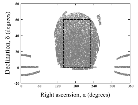
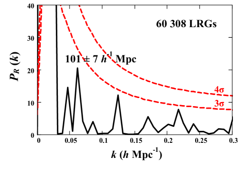
Figure 1: (Left panel): Angular distribution of LRGs over the sky from the SDSS DR7 data in the equatorial coordinate system; all grey colored regions comprise the DR7-Full sample in [35]; dashed lines delimit the rectangular region of our statistical consideration with $\alpha=140^{\circ}-230^{\circ}$ and $\delta=0^{\circ}-60^{\circ}$,  $\alpha$ and $\delta$ are defined about the axes, $\alpha$ is shown in a nonstandard way: east to right, west to left. (Right panel): Radial power spectrum $P_{R}(k)$ solid line calculated according to Equation (3) for all LRGs located in the rectangular region within the redshift interval $0.16\leq z\leq 0.47$  or distance interval $464\leq D(z)\leq 1274\leavevmode\nobreak\ h^{-1}$ Mpc. The significance levels $3\sigma$ and $4\sigma$ (dashed lines) are calculated using the mock LasDamas catalog and the exponential probability function (11) for random spectral peak amplitudes (see text)

Let us produce the next step that takes us beyond purely radial distributions. We scan the entire rectangle region by a trial sector with angular dimensions $5^{\circ}\times 25^{\circ}$ along right ascension and declination, respectively. At first, we build the radial distribution of LRGs precisely within the trial sector located in the angle range $\alpha=140^{\circ}\div 145^{\circ}$ and $\delta=0^{\circ}\div 25^{\circ}$, i.e., in the left lower corner of the rectangle region on the left panel of Figure 2. Using Equation (3), we calculate the 1D power spectrum $P_{R}(k)$ for the radial distribution of those LRGs, which were observed through this sector (as through a window) in the sky and strictly limited by the same redshift or distance intervals, as indicated in Section 2. Then we consequently shift this trial sector along the axes of right ascension or declination by five degrees and calculate the appropriate radial power spectra. In such a way, we consider 144 radial power spectra $P_{R}(k)$, which are non-overlapping along the horizontal axis but overlapping along the vertical one.

When analyzing the obtained spectra, we restrict ourselves to an interval $0.05<k<0.07$ and exploit the same procedure of significance assessment as it is described in Section 2 using the data of the mock LasDamas catalog. On the basis of these data, one can build the radial distributions and calculate power spectra within all of the outlined angular sectors. Among 144 sectors, we select only six, in which the significance of the peak amplitude exceeds $3\sigma$, and vary the angular boundaries of these sectors with a step $1^{\circ}$ to achieve maximum peak amplitudes. In this way, the appropriate angular dimensions of the six sectors were found to preserve the rectangular shape. After that, the 1D Fourier transform of the radial distributions of LRGs (already at $0<k\leq 0.3$) within their angular boundaries were produced. This allows us to calculate the scales and phases of quasi-periodic components in the selected cases.

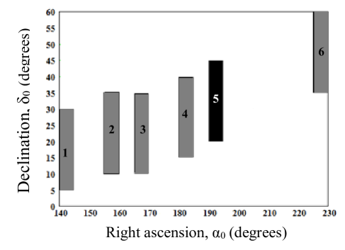
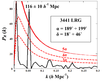
Figure 2: (Left panel): A total of 6 out of 144 sectors covering the entire rectangular area, which stand out due to their high peak amplitudes in the radial power spectra at $k_{\rm max}$, lying in a range $0.05\leq k_{\rm max}\leq 0.07\leavevmode\nobreak\ h$ Mpc^-1. (Right panel): Radial power spectrum $P_{R}(k)$ (solid line) calculated using Equation (3) for the black sector (No 5) in the left panel; dashed lines $-$ the significance levels $3\sigma$, $4\sigma$ and a narrow band $-$ $5\sigma$ calculated using the mock LasDamas catalog (see text); intervals of $\alpha$ and $\beta$ as well as the sample size are indicated in the insert

The six selected sectors are represented in the left panel of Figure 2, and their characteristics are shown in Table 1. The data include the sector numbers, the boundaries of angular variables, number of sampled LRGs, quasi-periods $\Delta D_{c}$ with errors determined as HWHM of the main spectral peaks and significance of the peaks.

Table 1: Data on six selected sectors with relatively high significance (Sign.) of the peaks in radial power spectra

No	$\alpha$	$\delta$	Number LRGs	Periods Mpc/$h$	Sign
1	$140^{\circ}$–$146^{\circ}$	$5^{\circ}$–$31^{\circ}$	2098	$101\pm 7$	$>$$3\sigma$
2	$154^{\circ}$–$160^{\circ}$	$8^{\circ}$–$39^{\circ}$	2434	$116\pm 10$	$>$$3\sigma$
3	$162^{\circ}$–$174^{\circ}$	$10^{\circ}$–$35^{\circ}$	3629	$116\pm 10$	$>$$5\sigma$
4	$182^{\circ}$–$185^{\circ}$	$15^{\circ}$–$41^{\circ}$	1121	$116\pm 10$	$>$$3\sigma$
5	$189^{\circ}$–$199^{\circ}$	$18^{\circ}$–$46^{\circ}$	3441	$116\pm 10$	$>$$5\sigma$
6	$222^{\circ}$–$230^{\circ}$	$36^{\circ}$–$60^{\circ}$	1634	$116\pm 10$	$>$$3\sigma$

Only sector No 1 in Figure 2 contains a quasi-periodical component with period $\Delta D_{c}=101\pm 7\leavevmode\nobreak\ h^{-1}$ Mpc  ($k_{\rm max}=0.062\pm 0.005\leavevmode\nobreak\ h$ Mpc^-1) at significance $>$$3\sigma$. The remaining five demonstrate significant peaks at $k_{\rm max}=0.054\pm 0.005\leavevmode\nobreak\ h$ Mpc^-1, corresponding to quasi-periodicity with a scale $\Delta D_{c}=116\pm 10\leavevmode\nobreak\ h^{-1}$ Mpc.

The right panel in Figure 2 shows the radial power spectrum calculated using the data of sector No 5 (black one in Figure 2). Note that the sector contains the north Galactic pole ($\alpha_{\rm np}=192.86^{\circ}$ and $\delta_{\rm np}=27.13^{\circ}$; see discussion in Section 6). In this case, we obtain the most prominent peak among all six sectors at the same $k_{\rm max}$ as the other five. The sample size is 3441 LRGs. The significance levels (also shown in the right panel) are estimated using the LasDamas catalog within the same sector on the sky. The dashed lines plot the significance levels $3\sigma$ and $4\sigma$, while the narrow band plots the level $5\sigma$ also calculated using (11) but for $A$ (see Equation (7)) lying within a $1\sigma$ error interval (in this case $A\simeq 160\pm 4$).

A single peak at $k=0.054\leavevmode\nobreak\ h\leavevmode\nobreak\ {\rm Mpc}^{-1}$ markedly exceeding $5\sigma$ is clearly visible in the power spectrum. This can serve as an additional justification for using Equation (11) to estimate the significance of separate peaks at different $k$ as a result of independent random fluctuations. Actually, smooth lines representing the significance levels on the right panel of Figure 2 and in the following figures are the locus of single peaks at fixed significance, calculated employing LasDamas data and the formulas (6)–(11) or their modifications (see Sections 4 and 5). On the other hand, it can be shown following [42, 46] as well as [47, 48] (and references therein) that the probability of occurrence of any number of random independent peaks for different $k$ leads to levels of significance not too different from that calculated with Equation (11) .

On the other hand, the power spectrum of the total normalized distribution of LRGs in all six selected sectors over the entire interval $0.04\leq k\leq 0.3\leavevmode\nobreak\ h$ Mpc^-1 does not contain significant peaks. This is similar to the spectrum obtained for the whole rectangle region and is plotted in the right panel of Figure 1. The small significance of the period 116 $h^{-1}$ Mpc is a consequence of the fact that these harmonics in the selected five sectors have different phases and mutually extinguish each other.

Random appearance and disappearance of the quasi-periodicity during the rotation of an observation field from sector to sector on the celestial sphere, as well as random phase shifts between the selected sectors, might indicate the existence of a sparse and ragged spatial structure at large cosmological distances. It may be assumed that radial distributions within wide angular regions are only capable of tracing such a structure indirectly. Below we develop a different approach for searching and analyzing such a possible structure and assessing its significance.

4 Cartesian Coordinate System. Preferred Direction

In this section, we refer to all three samples of LRGs presented in Section 1, DR7-Full, DR7-Dim and DR7-Bright, selected and described in [35] (see also [40]).

Let us move from spherical coordinates characterizing LRGs in Sections 2 and 3 to the distribution of the LRGs in Cartesian CS:

$$X_{i}=D(z_{i})\sin(90^{\circ}-\delta_{i})\cos\alpha_{i}$$ (12)

$$Y_{i}=D(z_{i})\sin(90^{\circ}-\delta_{i})\sin\alpha_{i}$$

$$Z_{i}=D(z_{i})\cos(90^{\circ}-\delta_{i}),$$

where $D(z_{i})$ is the radial comoving distance of $i$-th LRG with redshift $z_{i}$, $\alpha_{i}$ $-$ its right ascension and $\delta_{i}$ $-$ declination; in both the coordinate systems, an observer is at the zero point.

Following the definitions of Section 2, we use the binning approach along the axis $X$, and similar to calculations of $N_{R}(D_{c})$, we can calculate a distribution $N_{X}(X_{c})$, where $X_{c}$ is a central point of a bin, and $\Delta_{X}$ is its width. For the sample DR7-Full, we fix the same analyzed range $464\leq X\leq 1274\leavevmode\nobreak\ h^{-1}$ Mpc containing the same ${\cal N}_{b}=81$ independent bins with a width $\Delta_{X}=10\leavevmode\nobreak\ h^{-1}$ Mpc as it is used in  (2) for $D(z)$ (the intervals of DR7-Dim and DR7-Bright are considered below).

By analogy with Equation (2), we calculate the normalized 1D distribution along an axis $X$

$${\rm NN}_{X}(X_{c}^{l})={N_{X}(X_{c}^{l})-S_{X}\over\sqrt{S_{X}}},$$ (13)

where $l=1,2,\dots,{\cal N}_{b}$ is also the numeration of bins, and $S_{X}$ is a mean value of the 1D distribution $N_{X}(X_{c}^{l})$ over all bins.

Using Equations (3) and (13), one can calculate the 1D power spectrum $P_{X}(k_{m})$ replacing in (3) $D_{c}^{l}$ by $X_{c}^{l}$ and ${\rm NN}(D_{c}^{l})$ by ${\rm NN}_{X}(X_{c}^{l})$; in this case, $k_{m}=2\pi m/L_{X}$ is a wavenumber, $m=1,2,\dots,{\cal M}$ is a harmonic number, ${\cal M}=\lfloor{\cal N}_{b}/2\rfloor$ is a maximal number (the Nyquist number), and $L_{X}=810\leavevmode\nobreak\ h^{-1}$ Mpc is the whole interval along the axis $X$ (sampling length).

Then, we rotate the coordinate axes $XYZ$ at certain Euler angles so that the new axis $X^{\prime}$ would be oriented in a certain direction ($\alpha^{\prime}$ and $\delta^{\prime}$) relative to the initial Equatorial CS. Performing a sequence of such rotations, we search for the $X_{0}$-axis along which the 1D power spectrum calculated for all six sectors in total displays the most significant peak at a scale $\sim 116\leavevmode\nobreak\ h^{-1}$ Mpc.

To control the uniformity of statistics for different directions of $X$, we fix the same boundaries of the rotated axes, e.g.,  $464\leq X\leq 1274\leavevmode\nobreak\ h^{-1}$ Mpc for the sample DR7-Full. This condition strongly limits the area of analyzed directions  $160^{\circ}\leq\alpha\leq 200^{\circ}$ and $20^{\circ}\leq\delta\leq 40^{\circ}$ inside the rectangle. The same angular limits are set for the other two samples to ensure the same conditions in all cases under study. Employing the modification of Equation (3) described above, we calculate the 1D Fourier transform $F_{X}(k_{m})$ and the power spectra $P_{X}(k_{m})$ for each direction of $X$.

Actually, we deal with a discrete analog of so-called 3D Radon transform (e.g., [49]) applied to selected data, i.e., we summarize all the points from a subsample whose projections fall into each bin given along $X$. Thereafter, we exploit the two main properties of the Radon transform (i) translation invariance, which allows one to transfer the projections of the Cartesian galaxy coordinates on the given axis $X$ to another axis $\hat{X}$ parallel to the original one, (ii) linearity, which allows one to summarize the projections obtained for individual sectors in the sky into the total sum of projections to get a single Radon transform for the entire sample.

We start with an orientation of the $X$-axis along a direction with coordinates $\alpha=160^{\circ}$ and $\delta=20^{\circ}$ (lower left corner of the indicated region) and rotate the axis $X^{\prime}$ sequentially, shifting the right ascension or declination with a step $1^{\circ}$. Note that such rotations of the moving CS require only two Euler angles, $\alpha_{\rm Eu}=\Delta\alpha$ and $\beta_{\rm Eu}=\Delta\delta$, where $\Delta\alpha$ and $\Delta\delta$ are respective rotation angles. As a result, one can find an axis $X_{0}$ with Equatorial coordinates $\alpha_{0}$ and $\delta_{0}$ in the sky along which the 1D distribution of the Cartesian coordinate projections shows the maximum peak amplitude at $k$$\sim$0.05–0.06 $h$ Mpc^-1.

Table 2: SDSS LRG (DR7) and (DR12) statistics

Sample	Redshift	$X$ a   Mpc $h^{-1}$	Number LRGs	$\alpha_{0}$ b	$\delta_{0}$ b
DR7-Full c	$0.16\leq z\leq 0.47$	$464\leq X\leq 1274$	13 872	$176^{\circ}$	$24^{\circ}$
DR7-Dim c	$0.16\leq z\leq 0.36$	$464\leq X\leq 994$	8606	$177^{\circ}$	$22^{\circ}$
DR7-Bright c	$0.16\leq z\leq 0.44$	424 ${}^{f}\leq X\leq 1114$	4185	$177^{\circ}$	$23^{\circ}$
DR12-LOWZ ${}^{c,\ d}$	$0.16\leq z\leq 0.47$	$464\leq X\leq 1274$	38 880	$175^{\circ}$	$25^{\circ}$
DR12-SMASSLOWZE3 ${}^{c,\ d}$	$0.16\leq z\leq 0.72$	$464\leq X\leq 1844$	106 136	$176^{\circ}$	$27^{\circ}$
DR7-Full e	$0.16\leq z\leq 0.47$	$464\leq X\leq 1274$	57 099	$175^{\circ}$	$27^{\circ}$

a Intervals of galaxy Cartesian coordinate projections on any $X$-axis (see text).

b Equatorial coordinates of $X_{0}$-axes selected for each sample (see text).

c The data refer to the six sectors in the sky shown in Figure 2.

d Two samples from the DR12 data (see Section 5).

e The data refer to LRGs observed in the whole rectangular region

shown in Figure 1.

f Special case: $X\geq 424\leavevmode\nobreak\ h^{-1}$ Mpc at $z\geq 0.16$ (see text).

Table 2 gives the main characteristics of the subsamples used to find directions $X_{0}$ and to estimate the significance level of the main peak in each case. For all three subsamples, we perform rotations of the $X$-axis at fixed boundaries, $X_{\rm min}$ and $X_{\rm max}$ (different for each sample), providing uniformity of statistical conditions in different directions .

Figure 3 represents three distribution functions $N_{X}(X_{0})$ calculated as a number of cumulative projections on the axes $X_{0}$ (see Table 2 ) of Cartesian LRG coordinates registered through six sectors shown in the left panel of Figure 2. It is seen that all three curves have a quasi-oscillating character, i.e., represent an alternation of peaks and dips, the positions of a number of such features being mutually consistent.

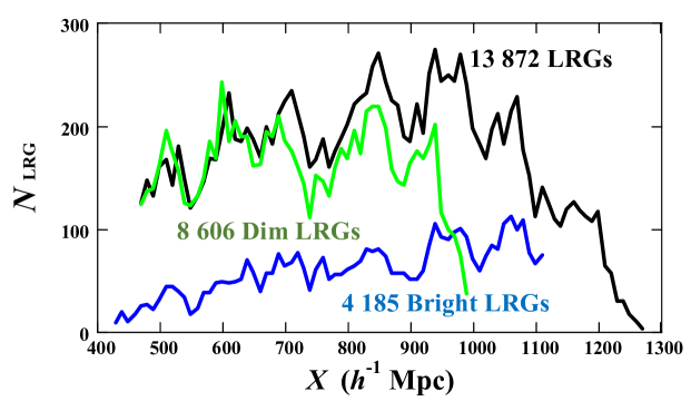
Figure 3: Three different distribution functions $N_{\rm LRG}\equiv N_{X}(X_{0})$ as a number of cumulative projections on a selected axis $X_{0}$ ($\alpha_{0}$, $\delta_{0}$; see text) of the Cartesian LRG coordinates detected through six sectors (windows) in the sky shown in Figure 2. Characteristics of all three samples, DR7-Full (black line), DR7-Dim (green line) and DR7-Bright (blue line), are given in Table 2

The results of our calculations of the 1D power spectrum are represented in Figures 4–6. The first two of them are based on data of the sample DR7-Full, while the third one — on data of the subsamples DR7-Dim and DR7-Bright. The first and third ones relate to all six sectors discussed above. The left panel in Figure 4 shows three confidence areas (shades of gray) on the sky indicating peak amplitudes (for the same scale $116\leavevmode\nobreak\ h^{-1}$ Mpc) exceeding the significance levels $3\sigma$ (light gray), $4\sigma$ (darker gray) and $5\sigma$ (dark), respectively. The maximum value of the peak is achieved along the direction of $X_{0}$ with coordinates $\alpha_{0}=176^{\circ}$ and $\delta_{0}=24^{\circ}$ (small white square).

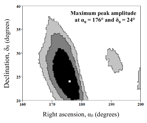
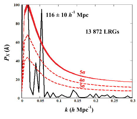
Figure 4: (Left panel): Areas of fixed confidence levels of the peaks in 1D power spectra $P_{X}(k)$ at $k_{\rm max}=0.054\leavevmode\nobreak\ h$ Mpc^-1 calculated using Cartesian LRG coordinates projected on various axes $X$; the data (corresponding to the sample DR7-Full) are collected for the six sectors shown in Figure 2; points in the $\alpha/\delta$-plane indicate the directions of axes. The colored areas are: light gray $-$ $(3\sigma)$, intermediate grey $-$ $(4\sigma)$ and dark grey $-$ $(5\sigma)$; the white square indicates the direction of the maximum spectral peak height ($\alpha_{0}$ and $\delta_{0}$). (Right panel): 1D power spectrum with maximum peak ($k=k_{\rm max}$) calculated for the projections on $X_{0}$-axis ( $\alpha_{0}$,  $\delta_{0}$) of the Cartesian LRG coordinates registered through the same six sectors; significance levels $3\sigma$ and $4\sigma$ (dashed lines) and the narrow band $5\sigma$ are plotted similarly to the levels and band in the right panel of Figure 2 (see text)

The right panel represents the power spectrum $P_{X}(k)$ calculated for normalized 1D distribution (13) of the LRG Cartesian coordinate projections on the $X_{0}$-axis with $\alpha_{0}$ and $\delta_{0}$ indicated above; the respective sample size is 13,872 LRGs. Two dashed lines show significance levels $3\sigma$ and $4\sigma$, while the narrow band (taking into account error bar $\pm 1\sigma$) corresponds to the level $5\sigma$ (in the case of Figure 4, we get $A=156\pm 6$), which are calculated in the same manner as described in Section 2 with the use of LasDamas catalog (“lrgFull-real”) for the same six sectors in the sky. We compute the ${\cal N}_{\rm LD}=80$ power spectra $P_{X}^{\rm LD}(k)$ produced for the normalized distributions (13) along the axis $X_{0}$. As a result, one can see that the dominant peak of our special interest far exceeds the level of $5\sigma$ and demonstrates an amplitude of about 100. This amplitude is noticeably larger than the similar peak in Figure 2.

Fourier analysis of these quasi-periodical components carried out separately for each selected sector shows that phases of the two most significant sectors (No 3 and 5 in the left panel of Figure 2, see also Table 1) get closer relative to the case of radial distributions. This phase convergence provides a major contribution to the cumulative spectrum of the six sectors in total.

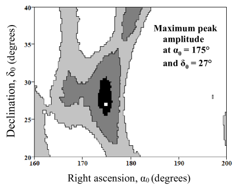
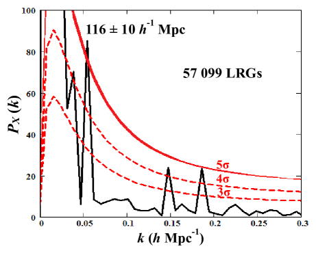
Figure 5: Same as the left and right panels of Figure 4, respectively, but for all of the data of the rectangle region shown in Figure 1. The maximum peak direction ($\alpha_{0}$ and $\delta_{0}$) practically coincides (slightly differs) with that in Figure 4 (see Table 2)

Figure 5 is organized similarly to Figure 4 but represents the results of calculations of 1D power spectra produced for the whole rectangle region shown in the left panel of Figure 1. The direction of the maximum amplitude of peaks in the power spectra $P_{X}(k)$ is only slightly shifted relative to the case of the six sectors in Figure 4, i.e., $\alpha_{0}=175^{\circ}$ and $\delta_{0}=27^{\circ}$.

The right panel represents the 1D power spectrum calculated along $X_{0}$ for a sample of 57,099 LRGs. One can see a strong peak at the same period $116\pm 10\leavevmode\nobreak\ h^{-1}$ Mpc but with an amplitude a bit lower than in the previous case. The significance levels (dashed lines and a narrow band) are constructed similar to the right panel in Figure 4 using LasDamas catalog (“lrgFull-real”) but for the whole rectangle region in the sky. This means that the proposed periodical structure oriented along $X_{0}$ can manifest itself even for the entire rectangle area under consideration (cf. with the right panel of Figure 1).

In both Figures 4 and 5, we can notice a smaller but also significant peak at lower $k<0.05\leavevmode\nobreak\ h$ Mpc^-1 and two significant peaks at $k\;\raise 1.29167pt\hbox{$<$\kern-7.5pt\raise-4.73611pt\hbox{$\sim$}}\;(0.15$–$0.2)\leavevmode\nobreak\ h$ Mpc^-1 in Figure 5. These features may indicate a more complex character of the structure under discussion than a single periodical dependence on $X$ but with a dominant role of the one highlighted component.

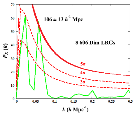
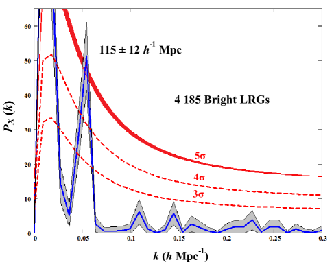
Figure 6: Same as the right panels of Figure 4 but for the subsamples DR7-Dim (left panel) and DR7-Bright (right panel); see Table 2 and text for details). The gray stripe near the power spectrum, plotted for DR7-Bright, demonstrates error bars, calculated by the jackknife technique

Figure 6 is organized in the same way as in the right panels in Figure 4 and deals only with the data of six chosen sectors. The figure is plotted for relatively more homogeneous samples DR7-Dim and DR7-Bright; the latter contains relatively fewer statistics. With this in mind, we slightly extended the low boundary of the $X_{0}$-projections in the case of DR7-Bright (at fixed $z=0.16$ as noted in the footnote No. 10), to increase the amplitude of the peak. However, we can argue that such variations of the boundary do not diminish the significance of the peak below $4\sigma$.

Moreover, following [50], we applied the jackknife procedure for the calculation of power spectrum error bands, obtained for DR7-Bright data (right panel). The stripe takes into account random variations of the data used for the calculation of the power spectrum. It can be seen that the errors cannot drastically affect the main peak significance.

Let us note that when considering the sample DR7-Bright, we do not use the reduction procedure (4) for calculating significance levels in the right panel of Figure 6, because the trend DR7-Bright turns out to be quite similar to the trend of mock LD data (catalog “lrg21p8-real”) selected under the same spatial conditions. This confirms the assumption that the reduction procedure introduced in Section 2 does not significantly affect the position and magnitude of the main peaks in the power spectra.

It is also worth noting that, based on the DR7-Bright sample, we compare two $N_{X}(X_{0})$ distributions constructed for the six sectors, as indicated in Figure 3, and for the entire rectangular region shown in Figure 1. Both distributions are similar and represent an alternation of peaks and dips; however, the amplitudes of these peaks and dips for the six sectors turned out to be a bit larger, which indicates some advantage of these sectors in tracing an assumed structure. The correlation coefficient of two curves is 0.51, which exceeds level $4\sigma$ for the considered volume of samples.

We can summarize that the celestial coordinates of the axes $X_{0}$ are quite close in all four cases under consideration (see Table 2). Moreover, the position and significance of the peaks in the right panels of Figures 4 and 5 and in both panels of Figure 6 are also mutually consistent. Thus, noticeable changes in the statistics and homogeneity of the samples do not significantly change the results, confirming their robustness.

In support of this statement, we introduce two auxiliary panels in Figure 7 showing weak dependence of the results on the degree of sample homogeneity. Indeed, the left panel of Figure 7 shows the effect of the window Fourier transform on the power spectrum obtained for the same distribution of the Cartesian coordinate projections on the axis $X_{0}$ as in the right panel of Figure 4. As a window function, we use the Hann function (e.g., [50, 51]):

$${\cal W}_{l}={1\over 2}\left[1-\cos\left({2\pi X_{c}^{l}\over L_{X}}\right)\right],$$ (14)

notations on the right-hand side are the same as in Equation (13).

The function (14) smooths the distribution of objects (points) along the edges of considered intervals, thereby suppressing the influence of sample inhomogeneities (visible, e.g., in Figure 3 for DR7-Full data) and smoothing out spurious periodicities induced by the boundaries of the intervals (e.g., [50]). On the other hand, this function strongly suppresses some of the useful information and, in particular, reduces traces of the periodic structure, if it is present, in the power spectrum (e.g., [51]).

We multiply the function (14) by the normalized distribution Equation (13), perform the Fourier transform of this product and construct the power spectrum following the modification of Equation (3) for projections onto the X-axis, as described above. Similarly, to obtain the significance levels shown in the left panel of Figure 7, we perform the same window Fourier transform of the one-dimensional distribution derived from the LasDamas data (the same catalog “lrgFull-real”).

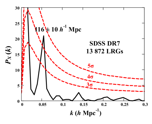
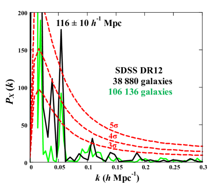
Figure 7: (Left panel): Same as the right panels in Figure 4 but with the inclusion of the Hann function (14) in the calculations of the window Fourier spectra (using the same DR7-Full data). (Right panel): Same as in the right panel of Figure 4 but using the data of SDSS DR12 related to the same six sectors in the sky. The green curve is the 1D power spectrum calculated for the extended interval $464\leq X\leq 1844\leavevmode\nobreak\ h^{-1}$ Mpc $(0.16\leq z\leq 0.72)$ of projections of the Cartesian galaxy coordinates on the axis $X_{0}$ ($\alpha_{0}=176^{\circ}$ and $\delta_{0}=27^{\circ}$, see Table 2) corresponding to the maximum peak at $k_{\rm max}=0.054\leavevmode\nobreak\ h$ Mpc^-1. The black curve is also a 1D power spectrum with the same $k_{\rm max}$ but calculated for the smaller interval $464\leq X\leq 1274\leavevmode\nobreak\ h^{-1}$ Mpc $(0.16\leq z\leq 0.47))$ used in Figures 4 and 5; in this case, $X_{0}$ is oriented along direction $\alpha_{0}=175^{\circ}$ and $\delta_{0}=25^{\circ}$; the sample sizes for both sets of data are also shown. The significance levels $3\sigma$, $4\sigma$ and $5\sigma$ (dashed lines ) are calculated for the extended sample of SDSS DR12 (see Section 5)

Comparing the left panel in Figure 7 with the right panel in Figure 4, one can notice the significant single peak at the same $k_{\rm max}=0.054\leavevmode\nobreak\ h$ Mpc^-1 but its amplitude is greatly reduced due to the influence of the window function on the power spectrum. However, the significance levels are also greatly reduced (slightly less than the peak amplitude), and the resulting significance does not fall below $4\sigma$, i.e., the peak remains quite significant.

5 Traces of Spatial Structure in SDSS DR12

To verify the results of Section 4, we probe the existence of a quasi-periodical structure on the basis of significantly expanded statistics of cosmologically distant galaxies accumulated in SDSS DR12. We consider these calculations as pure preliminary ones because here we do not take into account nonhomogeneity and selection effects of used data, do not study the wider sky area available for DR12, and in particular, are not looking for additional special sectors in the expanded region with significant spectral features, etc. Such calculations are the subject of future work. Here our task is only to establish whether there are contradictions between power spectra obtained along certain directions for quite different statistics presented in DR7 and DR12.

We employ the data of DR12 accumulated only for the northern hemisphere in the sky and collected in two files:
(1)  galaxy_ DR12v5 _ LOWZ _ North.fits.gz,  (2)  galaxy _ DR12v5 _ SMASSLOWZE3 _ North.fits.gz
which are available in the Science Archive Server . A description of the catalogs DR12 can be found, e.g., in [52-54].

One can produce calculations similar to those that are performed to plot Figure 4 using data related to the same six sectors in the sky, as presented in Table 1. We consider both an extended interval of redshifts $0.16\leq z\leq 0.72$ (SMASSLOWZE3) and the same (shorter) interval $0.16\leq z\leq 0.47$ (LOWZ) as it is studied in Sections 3 and 4. However, now our total sample contains 106,136 galaxies for the extended interval and 38,880 galaxies in the shorter interval (instead of 13,872 LRGs in Figure 4).

At first, we consider the extended redshift interval. As in the previous section, we choose the initial Cartesian CS and produce a lot of CS rotations within the same area in the sky $160^{\circ}\leq\alpha\leq 200^{\circ}$ and $20^{\circ}\leq\delta\leq 40^{\circ}$, as in Section 4. In this case, we restrict ourselves to a fixed interval $464\leq X\leq 1844\leavevmode\nobreak\ h^{-1}$ Mpc along each direction, similarly to how it is done for the DR7 data. For each direction of the $X^{\prime}$-axis, we also calculate the discrete analog of Radon transform, i.e., we summarize all the galaxies from a volumetric sample whose projections of the initial (fixed) Cartesian coordinates fall into a given bin along the rotating axis. In such a way, we obtain a 1D distribution $N_{X}(X_{c})$, where $X_{c}$ is the central point of a bin and, using Equation (13), produce the normalized distribution ${\rm NN}_{X}(X_{c})$.

This allows us to calculate the power spectra $P_{X}(k)$ for various $X^{\prime}$-axes and to find the direction of the maximum peak amplitude at $k_{\rm max}=0.054\leavevmode\nobreak\ h$ Mpc^-1. An example of such calculations for the direction of the maximum amplitude ($\alpha_{0}=176^{\circ}$ and $\delta_{0}=27^{\circ}$) is shown in the right panel of Figure 7 by the green curve. One can see that these coordinates are fairly close to the similar $\alpha_{0}$ and $\delta_{0}$ in Figure 4 (see also Table 2). The curve manifests a moderately high amplitude of the peak with a significance of $\sim$$4\sigma$.

Three dashed lines in the right panel of Figure 7 show significance levels $3\sigma$, $4\sigma$ and $5\sigma$, respectively. The calculations of these levels are carried out on the basis of the total sample (106,136 galaxies) by constructing a large number (${\cal{N}}_{X}$ = 861) of power spectra for various directions of $X^{\prime}$ evenly covering the area in the sky under investigation. Following Section 2, we obtain an averaged power spectra $\langle P_{X}(k)\rangle$, and using the Equations (5)–(7), (10) and (11), where all indices ${\rm LD}$ are replaced by $X$, we calculate the significance levels plotted in Figure 7 (right panel).

For comparison, the black curve demonstrates another example of the power spectrum calculations in the same interval $464\leq X\leq 1274\leavevmode\nobreak\ h^{-1}$ Mpc as it was used in Section 4. In this case, the full number of galaxies related to all six sectors reaches 38,880. As a result, we obtain a slightly different direction of the maximum amplitude ($\alpha_{0}=175^{\circ}$ and $\delta_{0}=25^{\circ}$) at the same $k_{\rm max}=0.054$. One can see that the amplitude of the dominant peak at the same $k_{\rm max}$ increases by approximately two times. On the other hand, the decrease of the peak amplitude for the extended interval of $X$ could be a consequence of the limited size of the quasi-periodical structure (if it exists) along the $X$-axis.

Thus, our preliminary analysis of DR12 data confirms an appearance of the significant feature at $0.05<k<0.07$ in the power spectra and thereby the possibility of existence of the quasi-periodic component oriented along the highlighted directions. Let us note that the narrow bunch of directions $X_{0}$ found in our study passes through the origin of CS (observer) by construction. However, we suppose that the real axis of periodicity could be (quasi-) parallel to the found axis (bunch of axes) and probably be shifted in space, so that the Radon transform does not change (see Section 4).

6 Conclusions and Discussion

The focus of this work is the search for traces of the anisotropic quasi-periodic structure in the spatial distribution of cosmological distant galaxies and application of a proper method for assessment of its significance. Summarizing the results obtained in Sections 3–5, we can hypothesize that at the considered redshifts, mainly at $0.16\leq z\leq 0.47$ (see also Table 2 for details), a large elongated quasi-periodic structure could exist with characteristic scale $\Delta X=116\pm 10\leavevmode\nobreak\ h^{-1}$ Mpc.

In order to specify the main axis of the structure, we perform the discrete 3D Radon transformations along various axes $X$ and calculate the power spectra for corresponding 1D distributions. One can imagine that the real axis of quasi-periodicity (if it exists) can be parallel to this axis but arbitrarily shifted in space. Such an approach may be treated as an application of the computer tomography elements to the analysis of the large-scale inhomogeneities of the matter (e.g., [55]) and possible signs of their quasi-periodicity.

Along special directions located within the narrow intervals of equatorial coordinates $\alpha_{0}\simeq 175^{\circ}-177^{\circ}$ and $\delta_{0}\simeq 22^{\circ}-27^{\circ}$, the structure is likely to have a maximum scale of  $>$$\sim$ 800 $h^{-1}$ Mpc. Our estimations show that a signal-to-noise ratio for the dominant spatial oscillations averaged over all selected directions indicated in Table 2 turned out to be $\sim$$2.0$, while a density contrast is $\sim$$0.1$ .

Among currently known large-scale structures in the spatial distribution of matter, the structure proposed here can be compared to the so-called Great Walls. To our knowledge, up to now a few Great Walls have been reliably established, and their number is constantly growing. These are the CfA Great Wall [56], Sloan Great Wall [57, 58], BOSS Great Wall [59] and Saraswati wall-like structure [60]. One can also refer to such objects as the supergalactic plane [61] in the local Universe, as well as the Sharpley Supercluster (e.g., [62, 63]), and the recently revealed South Pole Wall [64].

The structure proposed in the present work is about two or more times larger along the major axis than the appropriate scales of the Great Walls. Relative to $z$, the proposed structure is situated somewhere between the BOSS ($0.43<z<0.71$) and the Sloan Great Walls ($0.04<z<0.12$), and includes redshifts ($z\approx 0.3$) of the Saraswati Wall. The major axis of the assumed structure is directed relatively close to an area in the sky ($152^{\circ}\;\raise 1.29167pt\hbox{$<$\kern-7.5pt\raise-4.73611pt\hbox{$\sim$}}\;\alpha\;\raise 1.29167pt\hbox{$<$\kern-7.5pt\raise-4.73611pt\hbox{$\sim$}}\;170^{\circ},\ 44^{\circ}\;\raise 1.29167pt\hbox{$<$\kern-7.5pt\raise-4.73611pt\hbox{$\sim$}}\;\delta\;\raise 1.29167pt\hbox{$<$\kern-7.5pt\raise-4.73611pt\hbox{$\sim$}}\;58^{\circ}$) where the Boss Great Wall is located. The peculiarity of the structure discussed here is in its quasi-periodical character with low amplitude (or overdensity), which could be revealed only by specific techniques such as the anisotropic Fourier analysis employed in the present work.

In this regard, the question arises about the largest allowable scales of cosmological structures (huge superclusters and voids between them) consistent with the generally accepted $\Lambda$CDM cosmological model (e.g., [60]) with its extensive observation base. A possible answer to this question was given in [65], where it was shown that the largest structures of relatively low density can reach several hundred Megaparsecs without conflicting with the isotropy and uniformity of the $\Lambda$CDM model. However, in the literature, there is evidence (e.g., [66]) that the size of inhomogeneities in the distribution of cosmological matter can be much larger. Our estimates also show significantly larger dimensions of the anisotropic quasi-periodic structure. It means that the compatibility issue of such a scale with the currently dominant $\Lambda$CDM model remains open.

The same applies to the question of origin of the structure that we assume. It is quite likely, as suggested in [30], that the origin of anisotropic quasi-regular structures is associated with phase transitions during the inflation epoch or immediately after it. A possible way of solving the problem of the emergence of quasi-periodic structures in the early Universe was indicated in a recent work [67].

In addition, let us note that sector No 5 represented in the left panel of Figure 2 (see also Table 1) contains the direction to the north Galactic pole. In principle, the structure assumed here might be consistent with the pencil-beam quasi-periodicity at a scale $\sim$130 $h^{-1}$ Mpc found in the pencil-beam surveys near both Galactic poles (see [17] and a few references in the Introduction). It should be mentioned, however, that these results were criticized in the literature (e.g., in [68-70]) and perhaps the significance of periodicity was overestimated by the authors, who used the statistics available to them.

Actually, our analysis is different from the pencil-beam treatment, although in principle it may not contradict it. We analyze the projection of a volumetric array of points (LRGs) on selected directions, whereas the pencil-beam analysis has been produced for the distribution of galaxies along a set of narrow observational cones. Note that the directions along which there are significant peaks in the power spectra do not coincide with the direction to the Galactic pole. Moreover, Figure 5 shows the significant peak in the power spectrum calculated for a large number of LRG projections that were observed over the entire rectangular area in the sky, i.e., for LRGs collected from a huge spatial volume.

The structure proposed in the present work has a ragged character and can only appear in certain directions; moreover, different directions may trace over different visual space periodicities, as was found, e.g., in [29] and [30]. Nevertheless, two types of periodicities (one based on the pencil-beam analysis and the other one discussed in this article) might be interconnected, such as two different probes of the same complex quasi-regular structure.

Another point worth mentioning here is the closeness of the scale obtained in this work to both the characteristic scales of the quasi-regular structure formations and the BAO phenomenon (see Introduction). In our case, we are most likely dealing with an oriented anisotropic structure similar to those obtained in [17, 29] and [30]. Moreover, it seems to be plausible that the quasi-regular structure could manifest itself as several observed oscillations in space with a fixed scale (e.g., [17, 23, 30]), exactly as we find in this work.

As for the BAO, one can expect (see, e.g., [6]) that the primary perturbations in real space, associated with oscillations in k-space, could spread relative to their original centers (scattered isotropic) only within one acoustic wavelength. Such a concept of BAO has been confirmed to a certain degree by the calculations of [33]. Nevertheless, it is also possible that the proximity of the scales (for all their differences) of both types of phenomena under discussion is not accidental, and  they have common progenitors in primary perturbations at the early stages of the Universe evolution.

In any case, our hypothesis requires further detailed statistical studies, including an analysis of systematic errors that can lead to distortions of power spectra. This is especially true for DR12 data (Section 5), which must be used with great care. Our approach could be justified to some extent by the fact that the use of several samples with varying degrees of data heterogeneity and with varying degrees of accounting for systematic effects, leads to stable results. Nevertheless, it should be remembered that even with good statistics, low-quality data can lead to unreliable conclusions (see, e.g., [71]). In any case, all the effects considered here require further research, including the use of other catalogs of observational data. Moreover, these studies should be extended also to other areas in the sky, including the region of the south Galactic pole.

7 Acknowledgments

The authors are deeply grateful to the anonymous reviewers for many helpful and constructive comments.

References

- (1) Bond, J.R.; Kofman, L.; Pogosyan, D. How filaments of galaxies are woven into the cosmic web. Nature 1996, 380, 603–606.
- (2) Libeskind, N.I.; van de Weygaert, R.; Cautun, M.; Falck, B.; Tempel, E.; Abel, T.; Alpaslan, M.; Aragón-Calvo, M.A.; Forero-Romero, J.E.; Gonzalez, R.; et al. Tracing the cosmic web. Mon. Not. R. Astron. Soc. 2018, 473, 1195–1217.
- (3) van de Weygaert, R.; Schaap, W. The cosmic web: Geometric analysis. In Lecture Notes in Physics; Martínez, V.J., Saar, E., Martínez-González, E., Pons-Bordería, M.-J., Eds.; Data Analysis in Cosmology; Springer: Berlin, Germany, 2009; Volume 665, pp. 291–413.
- (4) Einasto, J. Dark Matter and Cosmic Web Story; Fang, L.Z., Ruffini, R., Eds.; Advanced Series in Astrophysics and Cosmology; World Scientific: Rome, Italy, 2014.
- (5) van de Weygaert, R. Voids and the Cosmic Web: Cosmic depression & spatial complexity. In The Zeldovich Universe: Genesis and Growth of the Cosmic Web; van de Weygert, R., Shandarin, S., Saar, E., Einasto, J., Eds.; IAU Symposium: Cambridge Univ. Press, 2016; Volume 308, pp. 493–523.
- (6) Eisenstein, D.J.; Seo, H.-J.; White, M. On the Robustness of the Acoustic Scale in the Low-Redshift Clustering of Matter. Astrophys. J. 2007, 664, 660–674.
- (7) Bassett, B.; Hlozek, R. Baryon acoustic oscillations. In Dark Energy; Ruiz-Lapuente, P., Eds. ; Cambridge Univ. Press, 2010; pp. 246–278.
- (8) Weinberg, D.H.; Mortonson, M.J.; Eisenstein, D.J.; Hirata, C.; Riess, A.G.; Rozo, E. Observational probes of cosmic acceleration. Phys. Rep. 2013, 530, 87–255.
- (9) Blake, C.; Glazebrook, K. Probing Dark Energy Using Baryonic Oscillations in the Galaxy Power Spectrum as a Cosmological Ruler. Astrophys. J. 2003, 594, 665–673.
- (10) Percival, W.J.; Cole, S.; Eisenstein, D.J.; Nichol, R.C.; Peacock, J.A.; Pope, A.C.; Szalay, A.S. Measuring the Baryon Acoustic Oscillation scale using the Sloan Digital Sky Survey and 2dF Galaxy Redshift Survey. Mon. Not. R. Astron. Soc. 2007, 3, 1053–1066.
- (11) Percival, W.J.; Reid, B.A.; Eisenstein, D.J.; Bahcall, N.A.; Budavari, T.; Frieman, J.A.; Fukugita, M.; Gunn, J.E.; Ivezić, Ž.; Knapp, G.R.; et al. Baryon acoustic oscillations in the Sloan Digital Sky Survey DR7 galaxy sample. Mon. Not. R. Astron. Soc. 2010, 401, 2148–2168.
- (12) Eisenstein, D.J.; Zehavi, I.; Hogg, D.W.; Scoccimarro, R.; Blanton, M.R.; Nichol, R.C.; Scranton, R.; Seo, H.-J.; Tegmark, M.; Zheng, Z.; et al. Detection of the Baryon Acoustic Peak in the Large-Scale Correlation Function of SDSS Luminous Red Galaxies. Astrophys. J. 2005, 633, 560–574.
- (13) Anderson, L.; Aubourg, É.; Bailey, S.; Beutler, F.; Bhardwaj, V.; Blanton, M.; Bolton, A.S.; Brinkmann, J.; Brownstein, J.R.; Burden, A.; et al. The clustering of galaxies in the SDSS-III Baryon Oscillation Spectroscopic Survey: baryon acoustic oscillations in the Data Releases 10 and 11 Galaxy samples. Mon. Not. R. Astron. Soc. 2014, 441, 24–62.
- (14) Kazin, E.A.; Koda, J.; Blake, C.; Padmanabhan, N.; Brough, S.; Colless, M.; Contreras, C.; Couch, W.; Croom, S.; Croton, D.J.; et al. The WiggleZ Dark Energy Survey: Improved distance measurements to z = 1 with reconstruction of the baryonic acoustic feature. Mon. Not. R. Astron. Soc. 2014, 441, 3524–3542.
- (15) Hong, T.; Han, J.L.; Wen, Z.L. A detection of Baryon Acoustic Oscillations from the distribution of galaxy clusters. Astrophys. J. 2016, 826, 154–161.
- (16) Alam, S.; Ata, M.; Bailey, S.; Beutler, F.; Bizyaev, D.; Blazek, J.A.; Bolton, A.S.; Brownstein, J.R.; Burden, A.; Chuang, C.-H.; et al. The clustering of galaxies in the completed SDSS-III Baryon Oscillation Spectroscopic Survey: cosmological analysis of the DR12 galaxy sample. Mon. Not. R. Astron. Soc. 2017, 470, 2617–2652.
- (17) Broadhurst, T.J.; Ellis, R.S.; Koo, D.C.; Szalay, A.S. Large-scale distribution of galaxies at the Galactic poles. Nature 1990, 343, 726–728.
- (18) Szalay, A.S.; Ellis, R.S.; Koo, D.C.; Broadhurst, T.J. Analysis of the large scale structure with deep pencil beam surveys. In After the First Three Minutes; Holt, S.S., Bennett, C.L., Trimble, V., Eds.; American Institute of Physics Conference Series, AIP Publishing LLC, Melvile, NY, USA ; 1991; pp. 261–275.
- (19) Szalay, A.S.; Broadhurst, T.J.; Ellman, N.; Koo, D.C.; Ellis, R.S. Redshift Survey with Multiple Pencil Beams at the Galactic Poles. Proc. Natl. Acad. Sci. USA 1994, 90, 4853–4858.
- (20) Koo, D.C.; Ellman, N.; Kron, R.G.; Munn, J.A.; Szalay, A.S.; Broadhurts, T.J.; Ellis, R.S. Deep pencil-beam redshift surveys as probes of large scale structures. In Observational Cosmology; Chincarini, G.L., Iovino, A., Maccacaro, T., Maccagni, D., Eds.; Astronomical Soc. Pac. Conf. Ser. , PASP, USA; 1993; Volume 51, pp. 112–118.
- (21) Einasto, M.; Einasto, J.; Tago, E.; Dalton, G.B.; Andernach, H. The structure of the universe traced by rich clusters of galaxies. Mon. Not. R. Astron. Soc. 1994, 269, 301–322.
- (22) Einasto, M.; Tago, E.; Jaaniste, J.; Einasto, J.; Andernach, H. The supercluster-void network I. The supercluster catalogue and large-scale distribution. Astron. Astrophys. Suppl. Ser. 1997, 123, 119–133.
- (23) Einasto, J.; Einasto, M.; Frisch, P.; Gottlober, S.; Muller, V.; Saar, V.; Starobinsky, A.A.; Tago, E.; Tucker, D.; Andernach, H. The supercluster-void network–II. An oscillating cluster correlation function. Mon. Not. R. Astron. Soc. 1997, 289, 801–812.
- (24) Einasto, J.; Einasto, M.; Frisch, P.; Gottlober, S.; Muller, V.; Saar, V.; Starobinsky, A.A.; Tucker, D. The supercluster-void network–III. The correlation function as a geometrical statistic. Mon. Not. R. Astron. Soc. 1997, 289, 813–823.
- (25) Einasto, J.; Einasto, M.; Gottlöber, S.; Müller, V.; Saar, V.; Starobinsky, A.A.; Tago, E.; Tucker, D.; Andernach, H.; Frisch, P. A 120-Mpc periodicity in the three-dimensional distribution of galaxy superclusters. Nature 1997, 385, 139–141.
- (26) Einasto, M.; Heinämäki, P.; Liivamägi, L.J.; Martínez, V.J.; Hurtado-Gil, L.; Arnalte-Mur, P.; Nurmi, P.; Einasto, J.; Saar, E. Shell-like structures in our cosmic neighbourhood. Astron. Astrophys. 2016, 587, A116–A124.
- (27) Yu, J.T.; Peebles, P.J.E. Superclusters of galaxies. Astrophys. J. 1969, 158, 103–113.
- (28) Webster, A. The clustering of radio sources–I. Mon. Not. R. Astron. Soc. 1976, 175, 61–70.
- (29) Landy, S.D.; Shectman, S.A.; Lin, H.; Kirshner, R.P.; Oemler, A.A.; Tucker, D. The Two-dimensional Power Spectrum of the Las Campanas Redshift Survey: Detection of Excess Power on 100 H -1 MPC Scales. Astrophys. J. Lett. 1996, 456, L1–L4.
- (30) Saar, E.; Einasto, J.; Toomet, O.; Starobinsky, A.A.; Andernach, H.; Einasto, M.; Kasak, E.; Tago, E. The supercluster-void network V. The regularity periodogram. Astron. Astrophys. 2002, 393, 1–23.
- (31) Ryabinkov, A.I.; Kaurov, A.A.; Kaminker, A.D. Quasi-periodical features in the distribution of Luminous Red Galaxies. Astrophys. Space Sci. 2013, 344, 219–228 (Paper I).
- (32) Ryabinkov, A.I.; Kaminker, A.D. Quasi-periodical components in the radial distributions of cosmologically remote objects. Mon. Not. R. Astron. Soc. 2014, 440, 2388–2395.
- (33) Arnalte-Mur, P.; Labatie, A.; Clerc, N.; Martínez, V.J.; Starck, J.-L.; Lachièze-Rey, M.; Saar, E.; Paredes, S. Wavelet analysis of baryon acoustic structures in the galaxy distribution. Astron. Astrophys. 2012, 542, A34–A44.
- (34) Ryabinkov, A.I.; Kaminker, A.D. Power-spectrum simulations of radial redshift distributions. Astrophys. Space Sci. 2019, 364, 129–140 (Paper II).
- (35) Kazin, E.A.; Blanton, M.R.; Scoccimarro, R.; McBride, C.K.; Berlind, A.A.; Bahcall, N.A.; Brinkmann, J.; Czarapata, P.; Frieman, J.A.; Kent, S.M.; et al. The Baryonic Acoustic Feature and Large-Scale Clustering in the Sloan Digital Sky Survey Luminous Red Galaxy Sample. Astrophys. J. 2010, 710, 1444–1461.
- (36) Berlind, A.A.; Frieman, J.; Weinberg, D.H.; Blanton, M.R.; Warren, M.S.; Abazajian, K.; Scranton, R.; Hogg, D.W.; Scoccimarro, R.; Bahcall, N.A.; et al. Percolation Galaxy Groups and Clusters in the SDSS Redshift Survey: Identification, Catalogs, and the Multiplicity Function. Astrophys. J. Suppl. Ser. 2006, 167, 1–25.
- (37) McBride, C.; Berlind, A.; Scoccimarro, R.; Wechsler, R.; Busha, M.; Gardner, J.; van den Bosch, F. LasDamas mock galaxy catalogs for SDSS. In American Astronomical Society Meeting Abstracts 213; Bulletin of the American Astronomical Society; Publishing AAS, Washington, DC, USA; 2009; Volume 41, p. 253.
- (38) Kayser, R.; Helbig, P.; Schramm, T. A general and practical method for calculating cosmological distances. Astron. Astrophys. 1997, 318, 680–686.
- (39) Hogg, D.W. Distance measures in cosmology. arXiv 1999, arXiv:astro-ph/9905116.
- (40) Zehavi, I.; Eisenstein, D.J.; Nichol, R.C.; Blanton, M.R.; Hogg, D.W.; Brinkmann, J.; Loveday, J.; Meiksin, A.; Schneider, D.P.; Tegmark, M. The Intermediate-Scale Clustering of Luminous Red Galaxies. Astrophys. J. 2005, 621, 22–31.
- (41) Jenkins, G.M.; Watts, D.G. Spectral Analysis and Its Applications; Holden-Day Series in Time Series Analysis; Holden-Day: London, UK, 1969.
- (42) Scargle, J.D. Studies in astronomical time series analysis. II–Statistical aspects of spectral analysis of unevenly spaced data. Astrophys. J. 1982, 263, 835–853.
- (43) Feldman, H.A.; Kaiser, N.; Peacock, J.A. Power-spectrum analysis of three-dimensional redshift surveys. Astrophys. J. 1994, 426, 23–37.
- (44) Bardeen, J.M.; Bond, J.R.; Kaiser, N.; Szalay, A.S. The statistics of peaks of Gaussian random fields. Astrophys. J. 1986, 304, 15–61.
- (45) Sugiyama, N. Cosmic Background Anisotropies in Cold Dark Matter Cosmology. Astrophys. J. 1995, 100, 281–305.
- (46) Frescura, F.A.M.; Engelbrecht, C.A.; Frank, B.S. Significance of periodogram peaks and a pulsation mode analysis of the Beta Cephei star V403Car. Mon. Not. R. Astron. Soc. 2008, 388, 1693–1707.
- (47) Lake, R.G.; Roeder, R.C. An analysis of the distribution of redshifts of quasars and emission-line objects. J. R. Astron. Soc. Can. 1972, 66, 111L–119L.
- (48) Newman, W.I.; Haynes, M.P.; Terzian, Y. Redshift data and statistical inference. Astrophys. J. 1994, 431, 147–155.
- (49) Deans, S.R. The Radon Transform and Some of Its Applications; Dover Publications, Inc.: New York, NY, USA, 2007.
- (50) Hawkins, E.; Maddox, S.J.; Merrifield, M.R. No periodicities in 2dF Redshift Survey data. Mon. Not. R. Astron. Soc. 2002, 336, L13–L16.
- (51) Napier, W.M.; Burbidge, G. The detection of periodicity in QSO data set. Mon. Not. R. Astron. Soc. 2003, 342, 601–604.
- (52) Bolton, A.S.; Schlegel, D.J.; Aubourg, É.; Bailey, S.; Bhardwaj, V.; Brownstein, J.R.; Burles, S.; Chen, Y.-M.; Dawson, K.; Eisenstein, D.J.; et al. Spectral Classification and Redshift Measurement for the SDSS-III Baryon Oscillation Spectroscopic Survey. Astron. J. 2012, 144, 144–166.
- (53) Alam, S.; Albareti, F.D.; Allende Prieto, C.; Anders, F.; Anderson, S.F.; Anderton, T.; Andrews, B.H.; Armengaud, E.; Aubourg, É.; Bailey, S.; et al. The Eleventh and Twelfth Data Releases of the Sloan Digital Sky Survey: Final Data from SDSS-III. Astrophys. J. Suppl. Ser. 2015, 219, 12–39.
- (54) Reid, B.; Ho, S.; Padmanabhan, N.; Percival, W.J.; Tinker, J.; Tojeiro, R.; White, M.; Eisenstein, D.J.; Maraston, C.; Ross, A.J.; et al. SDSS-III Baryon Oscillation Spectroscopic Survey Data Release 12: Galaxy target selection and large-scale structure catalogues. Mon. Not. R. Astron. Soc. 2016, 455, 1553–1573.
- (55) Starck, J.-L.; Martínez, V.J.; Donoho, D.L.; Levi, O.; Querre, P.; Saar, E. Analysis of the Spatial Distribution of Galaxies by Multiscale Methods. EURASIP J. Appl. Signal Process. 2005, 15, 2455–2469.
- (56) Geller, M.J.; Huchra, J.P. Mapping the Universe. Science 1989, 246, 897–903.
- (57) Gott, J.R., III; Jurić, M.; Schlegel, D.; Hoyle, F.; Vogeley, M.; Tegmark, M.; Bahcall, N.; Brinkmann, J. A Map of the Universe. Astrophys. J. 2005, 624, 463–484.
- (58) Einasto, M.; Lietzen, H.; Gramann, M.; Tempel, E.; Saar, E.; Liivamägi, L.J.; Heinämäki, P.; Nurmi, P.; Einasto, J. Sloan Great Wall as a complex of superclusters with collapsing cores. Astron. Astrophys. 2016, 595, A70–A82.
- (59) Lietzen, H.; Tempel, E.; Liivamägi, L.J.; Montero-Dorta, A.; Einasto, M.; Streblyanska, A.; Maraston, C.; Rubiño-Martín, J.A.; Saar, E. Discovery of a massive supercluster system at z 0̃.47. Astron. Astrophys. 2016, 588, L4–L8.
- (60) Bagchi, J.; Sankhyayan, S.; Sarkar, P.; Raychaudhury, S.; Jacob, J.; Dabhade, P. Saraswati: An Extremely Massive 200 Megaparsec Scale Supercluster. Astrophys. J. 2017, 844, 25–39.
- (61) Lahav, O.; Santiago, B.X.; Webster, A.M.; Strauss, M.A.; Davis, M.; Dressler, A.; Huchra, J.P. The supergalactic plane revisited with the Optical Redshift Survey. Mon. Not. R. Astron. Soc. 2000, 312, 166–176.
- (62) Bardelli, S.; Zucca, E.; Zamorani, G.; Moscardini, L.; Scaramella, R. A study of the core of the Shapley Concentration–IV. Distribution of intercluster galaxies and supercluster properties. Mon. Not. R. Astron. Soc. 2000, 312, 540–556.
- (63) Proust, D.; Quintana, H.; Carrasco, E.R.; Reisenegger, A.; Slezak, E.; Muriel, H.; Dünner, R.; Sodré, L.J.; Drinkwater, M.J.; Parker, Q.A.; Ragone, C.J. Structure and dynamics of the Shapley Supercluster. Velocity catalogue, general morphology and mass. Astron. Astrophys. 2006, 447, 133–144.
- (64) Pomarède, D.; Tully, R.B.; Graziani, R. Courtois, H.M.; Hoffman, Y.; Lezmy, J. Cosmicflows-3: The South Pole Wall. Astrophys. J. 2020, 897, 133–141.
- (65) Park, C.; Choi, Y.-Y.; Kim, J.; Gott, J.R., III; Kim, S.S.; Kim, K.-S. The Challenge of the Largest Structures in the Universe to Cosmology. Astrophys. J. Lett. 2012, 759, L7–L12.
- (66) Shirokov, S.I.; Lovyagin, N.Y.; Baryshev, Y.V.; Gorokhov, V.L. Large-scale fluctuations in the number density of galaxies in independent surveys of deep fields. Astron. Rep. 2016, 60, 563–577.
- (67) Voskresensky, D.N. Evolution of Quasiperiodic Structures in a Non-Ideal Hydrodynamic Description of Phase Transitions. Universe 2020, 6, 42–56.
- (68) Kaiser, N.; Peacock, J.A. Power-spectrum analysis of one-dimensional redshift surveys. Astrophys. J. 1991, 379, 482–505.
- (69) Eisenstein, D.J.; Hu, W.; Silk, J.; Szalay, A.S. Can Baryonic Features Produce the Observed 100 h-1 Mpc Clustering? Astrophys. J. Lett. 1998, 494, L1–L4.
- (70) Yoshida, N.; Colberg, J.; White, S.D.M.; Evrard, A.E.; MacFarland, T.J.; Couchman, H.M.P.; Jenkins, A.; Frenk, C.S.; Pearce, F.R.; Efstathiou, G.; et al. Simulations of deep pencil-beam redshift surveys. Mon. Not. R. Astron. Soc. 2001, 325, 803–816.
- (71) Efstathiou, G.; Lemos, P. Statistical inconsistencies in the KiDS-450 data set. Mon. Not. R. Astron. Soc. 2018, 476, 151–157.