Fluid descriptions of quantum plasmas

Abstract

Quantum fluid (or hydrodynamic) models provide an attractive alternative for the modeling and simulation of the electron dynamics in nano-scale objects. Compared to more standard approaches, such as density functional theory or phase-space methods based on Wigner functions, fluid models require the solution of a small number of equations in ordinary space, implying a lesser computational cost. They are therefore well suited to study systems composed of a very large number of particles, such as large metallic nano-objects. They can be generalized to include the spin degrees of freedom, as well as semirelativistic effects such as the spin-orbit coupling. Here, we review the basic properties, advantages and limitations of quantum fluid models, and provide some examples of their applications.

1 Introduction – Fluid models for classical and quantum plasmas

Recent decades have witnessed a remarkable surge of interest for the electronic properties of nano-scale objects, particularly when excited by electromagnetic radiation Voisin2000 ; Bigot2000 ; Manfredi2018SPIE ; Maniyara2019 . This is a very vast domain of research that encompasses all sorts of nano-objects (metallic films and nanoparticles, carbon nanotubes, semiconductor quantum dots …), new materials like graphene, as well as meta-materials whose structure can be engineered so as to display some particular electromagnetic properties. Potential applications are impressive, and range from high-performance computing (efficient storage and transfer of information), to nanoplasmonics Stockman2011 ; Moreau2012 (optical filters, waveguides), and even to the medical sciences (biomedical tests and sensors) Hainfeld2004 ; TatsuroEndo2006 .

The electronic response of such systems (often in the out-of-equilibrium and nonlinear regimes) can be assimilated to that of a one-component quantum plasma and may be treated at different levels of approximations. For systems containing many interacting electrons, condensed-matter physicists and quantum chemists have developed various theoretical strategies, such as the time-dependent density functional theory (TDDFT) and time-dependent Hartree-Fock (TDHF) methods. TDDFT and TDHF are wavefunction-based methods, but they can be reformulated in the phase-space language familiar to plasma physicists by making use of Wigner functions. In a recent work Manfredi2019 , we reviewed the use of phase-space methods for applications to condensed matter and nanophysics. The first chapters of that work also discuss some general properties of solid-state plasmas.

Both approaches (wavefunction and phase space) are rather costly in terms of run-time and memory storage, especially for systems containing thousands of electrons. A possible, less costly alternative is provided by fluid models, which can be derived from the corresponding kinetic equations (Wigner for a fully quantum approach, or Vlasov for semiclassical modeling) by taking velocity moments of the distribution function Manfredi2001 . Although some information is inevitably lost in this procedure, one can expect the fluid approach to be accurate enough to provide key insights on the underlying physical mechanisms, while at the same time remaining affordable in terms of computational cost. Like their classical counterparts, the validity of quantum fluid models is restricted to long wave lengths compared to the interparticle distance Khan2014 . However, they can deal with nonlinear effects (large excitations), quantum effects (tunnelling), Coulomb exchange (an effect related to the Pauli exclusion principle), and electron-electron correlations.

In the fluid approach, the electron dynamics is described by a set of hydrodynamic equations (continuity, momentum balance, energy balance) that include quantum effects via the so-called Bohm potential. A considerable gain in computing time can be expected in comparison to Wigner or TDDFT simulations: indeed, TDDFT methods must solve $N\gg 1$ Schrödinger-like equations, while the phase space approach doubles the number of independent variables (positions and velocities). Hydrodynamic models were used in the past in condensed-matter physics, particularly for semiconductors Muller2004 and, to a lesser extent, metal clusters Domps1998 ; Banerjee2000 . More recently, the quantum fluid description has been extended to include another important property of the electron, namely its spin Brodin2007 . The resulting fluid equations are much more involved that their spinless counterparts, but may find useful applications, in condensed-matter physics, to the emerging field of spintronics Hirohata2020 , and in plasma physics to the study of highly polarized electron beams Wu2019 ; Wu2020 . Quantum fluid theory finds further applications to the dense plasmas produced in the interaction of solid targets with intense laser beams Kremp2001 , to warm dense matter experiments Dornheim2018 ,

to quantum nanoplasmonics Ciraci2013 ; Ciraci2016 ; Ciraci2021 ; Toscano2015 , and to compact astrophysical objects such as white dwarf stars Uzdensky2014 .

The purpose of this short review is to present the results on quantum fluid models obtained in our research group at the University of Strasbourg during the last two decades. The bibliography on quantum plasmas has grown immensely during this period and it is hardly possible to do justice to all works on this topic. A recent paper Bonitz2019 has tried to summarize the status of present quantum fluid theory, as well as the prospects for future developments.

The present work is organized as follows. In section 2 we derive the fluid equations in the simplest case and describe their properties. In section 3 we discuss the range of validity of the fluid approach. In particular, the closure relations are analyzed by comparing the fluid and kinetic dispersion relations in two regimes of interest: fast Langmuir waves and slow ion acoustic waves. Section 4 contains a practical example of application of quantum fluid theory to plasmonic oscillations in a metallic nanoshell. Section 5 generalizes the fluid equations to take into account the electron spin. More advanced semirelativistic effects, such as the spin-orbit coupling, are also considered. In section 6 we discuss a variational formulation of the quantum fluid equations through an appropriate Lagrangian. The variational approach enables us to reduce the full fluid description to a set of a few ordinary differential equations, which can then be solved either analytically or numerically with little computational cost. Some applications to electronic modes in semiconductor quantum wells are also illustrated.

2 Quantum fluid models without spin

For a classical collisionless plasma, the electron dynamics is fully described by a probability distribution in the phase space $f(\bm{r},\bm{p},t)$, evolving in time according to the Vlasov equation. For a quantum electron gas, the corresponding statistical tool is the density matrix:

$$\rho(\bm{r},\bm{r}^{\prime})=\sum_{\alpha=1}^{N}p_{\alpha}\Psi_{\alpha}^{\displaystyle*}(\bm{r})\Psi_{\alpha}(\bm{r}^{\prime}),$$ (1)

where $p_{\alpha}$ is the probability to be in the state $\Psi_{\alpha}$. In order to make contact with classical plasma physics, it is useful to introduce the Wigner distribution function, defined as

$$f\left(\bm{r},\bm{p},t\right)=\frac{1}{\left(2\pi\hbar\right)^{3}}\int d\bm{\lambda}\exp\left(\frac{i\bm{p}\cdot\bm{\lambda}}{\hbar}\right)\rho\left(\bm{r}+\frac{\bm{\lambda}}{2},\bm{r}-\frac{\bm{\lambda}}{2},t\right).$$ (2)

The Wigner function evolves in time according to the following Wigner equation

$$\frac{\partial f}{\partial t}+\frac{\bm{p}}{m}\cdot\bm{\nabla}f=\displaystyle\frac{ie}{\hbar}\frac{1}{\left(2\pi\hbar\right)^{3}}\int d\bm{\lambda}d\bm{p^{\prime}}e^{\frac{i\left(\bm{p}-\bm{p^{\prime}}\right)\cdot\bm{\lambda}}{\hbar}}\left[V(\bm{r}_{+})-V(\bm{r}_{-})\right]f(\bm{r},\bm{p^{\prime}},t).$$ (3)

where $e>0$ and $m$ are the electron charge and mass respectively, the indices $\bm{\pm}$ denote the shifted positions $\bm{r}_{\pm}=\bm{r}\pm\bm{\lambda}/2$, and the potential $V(\bm{r},t)$ is either an external potential or a self-consistent potential obtained from Poisson’s equation (or the sum of both).

The Wigner approach allows one to recast the dynamics of a quantum electron gas in the familiar formalism of the classical phase space. But it should not be forgotten that the Wigner function, although real, can take negative values, and is therefore not a true probability distribution like its classical counterpart. Two comprehensive reviews of the Wigner phase-space methods applied to the description of quantum plasmas were published recently in this journal Manfredi2019 ; Melrose2020 , to which we refer the reader for further details.

Fluid, or hydrodynamic, models are usually obtained by taking moments of the relevant phase-space distribution (Vlasov or Wigner). Thus, the $k$-th order moment is defined as:

$$\textsf{m}_{k}(\bm{r},t)\equiv\int f(\bm{r},\bm{p},t)\,\underbrace{\bm{p}\otimes\bm{p}\dots\otimes\bm{p}}_{k\,\rm times}\,d\bm{p},$$ (4)

where the symbol $\otimes$ denotes the tensor product. Clearly, $\textsf{m}_{k}$ is a tensor of rank $k$. Each moment obeys an evolution equation, which can be interpreted as a conservation law for a given physical quantity (mass, momentum, energy, etc…). The evolution equation for the moment of order $k$ generally depends on the equation for the moment of order $k+1$, thus forming an infinite hierarchy of equations. Hence, some further assumptions are needed in order to close this infinite system. Here, we will essentially consider two-moment fluid systems, based on the evolution of the electron density $n(\bm{r},t)$ (zeroth order moment):

$$\int fd\bm{p}=\sum_{\alpha=1}^{N}p_{\alpha}\Psi_{\alpha}^{*}\left(\bm{r},t\right)\Psi_{\alpha}\left(\bm{r},t\right)\equiv n\left(\bm{r},t\right),$$ (5)

and the electron current $\bm{j}(\bm{r},t)$ (first order moment):

$$\int\bm{p}fd\bm{p}=\frac{i\hbar}{2}\sum_{\alpha=1}^{N}p_{\alpha}\left[\Psi_{\alpha}\left(\bm{r},t\right)\bm{\nabla}\Psi_{\alpha}^{*}\left(\bm{r},t\right)-\Psi_{\alpha}^{*}\left(\bm{r},t\right)\bm{\nabla}\Psi_{\alpha}\left(\bm{r},t\right)\right]\equiv\bm{j}\left(\bm{r},t\right).$$ (6)

A generalization of this procedure to higher order moments was also developed Haas2010 .

By integrating the Wigner equation (3) over the momentum variable, we obtain the continuity equation (conservation of mass):

$$\frac{\partial n}{\partial t}+\bm{\nabla}\cdot\left(n\bm{u}\right)=0,$$ (7)

where we used the mean velocity $\bm{u}(\bm{r},t)\equiv\bm{j}(\bm{r},t)/n(\bm{r},t)$. Multiplying the Wigner equation by $\bm{p}$ and integrating yields the evolution equation for the mean velocity (momentum conservation law):

$$\frac{\partial u_{i}}{\partial t}+u_{j}(\partial_{j}u_{i})=-\frac{1}{nm}\partial_{j}\textsf{P}_{ij}+\frac{e}{m}\partial_{i}{V},$$ (8)

where we adopted the Einstein summation convention over repeated indices (this will be used systematically in the rest of this work). Note that Eq. (8) has the same form as the Euler equation in standard hydrodynamics.

The pressure tensor $\textsf{P}_{ij}$ is a second-order moment of the distribution function defined as

$$\textsf{P}_{ij} =\int w_{i}w_{j}fd\bm{p},$$ (9)

where we separated the mean fluid velocity $\bm{u}$ from the velocity fluctuations $\bm{w}\equiv\bm{v}-\bm{u}$. To obtain the evolution equation of the pressure tensor, one should take the second order moment of the Wigner equations, which would contain the third-order moment (energy flux), and so on and so forth. As we are aiming at a two-moment fluid model, we should try to obtain some closure relation that allows us to express $\textsf{P}_{ij}$ as a function of the lower order moments $n$ and $\bm{u}$.

A simple closure can be achieved by writing the pressure tensor in terms of the electronic wave functions. Using Eqs. (2) and (9) and after some algebra, one is able to write the pressure tensor as follows:

$$\textsf{P}_{ij}= \frac{\hbar^{2}}{4m}\sum_{\alpha}p_{\alpha}\left[\left(\partial_{i}\Psi_{\alpha}^{*}\right)\left(\partial_{j}\Psi_{\alpha}\right)+\left(\partial_{j}\Psi_{\alpha}^{*}\right)\left(\partial_{i}\Psi_{\alpha}\right)-\Psi_{\alpha}^{*}\left[\partial_{i}\left(\partial_{j}\Psi_{\alpha}\right)\right]-\Psi_{\alpha}\left[\partial_{i}\left(\partial_{j}\Psi_{\alpha}^{*}\right)\right]\right]$$

$$~{}+\frac{\hbar^{2}}{4mn}\left[\sum_{\alpha}p_{\alpha}\left[\Psi_{\alpha}^{*}\left(\partial_{i}\Psi_{\alpha}\right)-\Psi_{\alpha}\left(\partial_{i}\Psi_{\alpha}^{*}\right)\right]\left[\Psi_{\alpha}^{*}\left(\partial_{j}\Psi_{\alpha}\right)-\Psi_{\alpha}\left(\partial_{j}\Psi_{\alpha}^{*}\right)\right]\right]^{2}.$$ (10)

In order to interpret this pressure tensor, we shall use the Madelung decomposition Madelung1927 :

$$\Psi_{\alpha}(\bm{r},t) =A_{\alpha}(\bm{r},t)\exp\left(\frac{iS_{\alpha}(\bm{r},t)}{\hbar}\right),$$ (11)

where $A_{\alpha}(\bm{r},t)$ is the amplitude of the wave function and $S_{\alpha}(\bm{r},t)$ its phase, both being real functions.

The individual particle density and velocity for each wave function are defined as:

$$n_{\alpha}(\bm{r},t) =A_{\alpha}^{2}(\bm{r},t),~{}~{}~{}~{}\bm{u}_{\alpha}(\bm{r},t)=\frac{1}{m}\bm{\nabla}S_{\alpha}(\bm{r},t).$$ (12)

The connection with the global fluid variables $n$ and $\bm{u}$, derived from the Wigner approach, is made by taking the statistical average of Eqs. (12), to obtain

$$n =\sum_{\alpha=1}^{N}p_{\alpha}n_{\alpha}~{}~{}~{}~{}\textrm{and}~{}~{}~{}~{}\langle\bm{u}_{\alpha}\rangle\equiv\bm{u}=\frac{1}{n}\sum_{\alpha=1}^{N}p_{\alpha}n_{\alpha}\bm{u}_{\alpha}.$$ (13)

Then using, Eqs. (11)-(13), one obtains a simpler form for the pressure tensor:

$$\textsf{P}_{ij} =mn\left(\langle u_{i}u_{j}\rangle-\langle u_{i}\rangle\langle u_{j}\rangle\right)$$

$$+\frac{\hbar^{2}}{2m}\sum_{\alpha}p_{\alpha}\left[\left(\partial_{i}\sqrt{n_{\alpha}}\right)\left(\partial_{j}\sqrt{n_{\alpha}}\right)-\sqrt{n_{\alpha}}\left(\partial_{i}\left(\partial_{j}\sqrt{n_{\alpha}}\right)\right]\right]\equiv\textsf{P}^{C}_{ij}+\textsf{P}^{Q}_{ij}.$$ (14)

The first term of the right-hand side ($\textsf{P}^{C}_{ij}$) has the form of a velocity dispersion, i.e., the same form as the standard definition of the pressure tensor in an ordinary classical gas. It is a statistical term which disappears for a pure quantum state, i.e., when only one quantum state is occupied in Eq. (1). Hence, we can use our knowledge of classical fluid dynamics to obtain appropriate closures for this “classical” pressure term. For instance, for an isotropic Maxwell-Boltzmann equilibrium at constant temperature $T_{e}$ (isothermal transformation), one would have: $\textsf{P}^{C}_{ij}=\delta_{ij}P[n]$, with $P[n]=nk_{B}T_{e}$, where $k_{B}$ is the Boltzmann constant and $\delta_{ij}$ is the Kronecker delta. For an ideal and fully degenerate electron gas, this “classical” and isotropic pressure would coincide with the Fermi degeneracy pressure Ashcroft2002 :

$$P[n]=\frac{\left(3\pi^{2}\right)^{2/3}\hbar^{2}}{5m}n^{5/3}.$$ (15)

The above examples are simple instances of equations of state (EOS).

The second term of the right side is proportional to Planck’s constant $\hbar$, hinting at its quantum origin. Indeed, this quantum pressure term $\textsf{P}^{Q}_{ij}$ has no classical counterpart and subsists even when only one state is occupied in Eq. (1), i.e. for a pure quantum state. Physically, it originates from the Heisenberg uncertainty principle, which forbids that a quantum particle possesses a definite velocity, except if its position is completely delocalized. For instance, it is in virtue of this “quantum” pressure that the ground state of a quantum harmonic oscillator has a finite velocity dispersion, unlike a classical oscillator.

An exact closure for the quantum pressure can be found under the (rather restrictive) assumption that the amplitudes of all the wave functions are identical, i.e. $n_{\alpha}(\bm{r},t)=n(\bm{r},t),\,\forall\alpha$ Manfredi2005 . In this case one obtains:

$$\textsf{P}^{Q}_{ij} =\frac{\hbar^{2}}{2m}\left[\left(\partial_{i}\sqrt{n}\right)\left(\partial_{j}\sqrt{n}\right)-\sqrt{n}\left[\partial_{i}\left(\partial_{j}\sqrt{n}\right)\right]\right].$$ (16)

To simplify even more, one can assume the isotropy of the pressure, i.e. $\textsf{P}^{Q}_{ij}=P^{Q}\,\delta_{ij}$, yielding

$$P^{Q}[n]=\frac{\hbar^{2}}{2m}\left[(\bm{\nabla}\sqrt{n})^{2}-\sqrt{n}\,\bm{\nabla}^{2}(\sqrt{n})\right]$$ (17)

where we have indeed expressed $P^{Q}$ in terms of the electron density and its derivatives. This completes the closure procedure. We also note that the quantum pressure (17) can be rewritten in the form of a potential, by noting that

$$\frac{\bm{\nabla}P^{Q}}{m}=\bm{\nabla}V_{B},$$ (18)

where $V_{B}$ is the Bohm potential Bohm1952 , defined as:

$$V_{B}=-\frac{\hbar^{2}}{2m}\frac{\bm{\nabla}^{2}\sqrt{n}}{\sqrt{n}}.$$ (19)

However, we note that the hypothesis of identical amplitudes for all the wave functions, although certainly sufficient to obtain an exact closure of the quantum pressure term, is by no means necessary for approximate closures. Indeed, the Bohm potential is in reality a quantum correction to the electron kinetic energy Michta2015 , as was already noticed by von Weizsäcker many years ago Weizsacker1935 . It can be derived from the standard Thomas-Fermi theory including gradient corrections, and it appears as the first gradient correction beyond the local density approximation. As a gradient correction, it disappears for a homogeneous density profile and is small for weak spatial modulations (long wave lengths). This suggests that the closure (17) is approximately correct for density gradients that are not too strong. A simple dimensional analysis shows that, for an electron gas at zero temperature, the scale length beyond which this closure is acceptable must be of the order of the Thomas-Fermi screening length $\lambda_{TF}=\sqrt{2\varepsilon_{0}E_{F}/(e^{2}n_{0})}$, where $e$ is the absolute electron charge, $\varepsilon_{0}$ is the dielectric constant in vacuum, $n_{0}$ is a reference number density, and $E_{F}=\frac{\hbar}{2m}\left(3\pi^{2}n_{0}\right)^{2/3}$ is the Fermi energy.

Then, using the closure relations for the classical pressure (15) and the quantum pressure (17), one can rewrite the fluid equations (7) and (8) in the closed form:

$$\begin{array}[]{lcl}\displaystyle\displaystyle\frac{\partial n}{\partial t}+\bm{\nabla}\cdot\left(n\bm{u}\right)=0,\\ \\ \displaystyle\frac{\partial u_{i}}{\partial t}+u_{j}(\partial_{j}u_{i})=\frac{\hbar^{2}}{2m^{2}}\partial_{i}\left[\frac{\bm{\nabla}^{2}\sqrt{n}}{\sqrt{n}}\right]-\frac{1}{nm}\partial_{i}P+\frac{e}{m}\partial_{i}{V}.\end{array}$$ (23)

The above quantum fluid equations (23) are usually referred to as the quantum hydrodynamic (QHD) model. The potential $V(\bm{r},t)$ can often be written as the sum of an external potential $V_{ext}$ and a self-consistent Hartree potential $V_{H}$, which is a solution of the Poisson equation

$$\bm{\nabla}^{2}V_{H}=en/\varepsilon_{0}.$$ (24)

Equations (23)-(24) constitute a useful semiclassical mean-field model to treat the electron dynamics of a degenerate electron gas, simpler to implement numerically than the corresponding Wigner equation. They were used, for instance, to study the nonlinear electrons dynamics in metallic films Crouseilles2008 or, more recently, monopole plasmon oscillations in a $\rm C_{60}$ molecule Tanjia2018 and in a metallic nanoshell Tanjia2018 .

Further, the total potential $V$ in Eq. (23) can be augmented to include non-ideal effects such as electronic correlations and the exchange interaction.

The exchange interaction stems from the fact that the many-body wave function of a system of uncorrelated fermions is not simply the product of single-particle wave functions, but rather has the form of a Slater determinant. This guarantees that the many-body wave function is antisymmetric (changes sign when two particles are interchanged), as it should be for fermions Manfredi2019 . Both exchange and correlations can be included in the fluid models, following the approach of density functional theory (DFT), by defining appropriate potentials $V_{C}[n]$ and $V_{X}[n]$ that depend functionally on the electron density. The simplest choice is the so-called local density approximation (LDA) Kohn1965 , whereby the exchange and the correlation functionals depend locally on the electron density. For instance, the LDA approximation for the exchange potential is:

$$V_{X}[n]=-\frac{e^{2}}{4\pi\epsilon_{0}}\left(\frac{3}{\pi}\right)^{1/3}n^{1/3}.$$ (25)

More sophisticated functionals have been designed to describe electron correlations in the transition region between the bulk and the outer surface of a nano-object Armiento2005 . Many other approximate functionals have been developed over the years (such as the generalized gradient approximation, GGA), making DFT methods a cornerstone of computational materials science and theoretical chemistry Jones2015 .

A recent benchmarking study compared the performances of various commonly used exchange-correlation functionals regarding their ability to describe electronic systems under external harmonic perturbations with different amplitudes and wave-numbers Moldabekov2021b . These functionals can be used in fluid models to extend their validity beyond the mean-field approximation.

Alternatively, the exchange interaction can be taken into account in a phase-space description, such as the Wigner or Vlasov equations. As the exchange is a two-body effect (beyond mean field), one must include corrections brought about by the two-body distribution function to derive a suitable kinetic equation Zamanian2013 . Next, one can follow the same moment-taking procedure as above to obtain a set of fluid equations that include the electron exchange interaction, as was done very recently in Ref. Haas2021 .

Finally, we note that the fluid equations (23) can be viewed as a time-dependent generalization of the early Thomas-Fermi theory of the atomic electron gas Thomas1926 . Indeed, taking $\partial/\partial t=0$ and $\bm{u}=0$ everywhere, and neglecting the quantum term (i.e., the Bohm potential), one gets:

$$-\frac{\nabla P}{n}+e\nabla V_{H}+e\nabla V_{ext}=0.$$

Using Eq. (15), and defining the chemical potential $\mu$ as an integration constant, we obtain

$$-\frac{\hbar^{2}}{2m}(3\pi^{2}n)^{2/3}+eV_{H}[n]+eV_{ext}=\mu,$$ (26)

which is an integral equation for the ground-state density $n$ and is identical to the standard Thomas-Fermi equation Michta2015 .

3 Validity of quantum fluid models

3.1 Closure relations

As we have seen in the preceding section, the fluid equations need two further closure relations in order to form closed system – one for the classical pressure and one for the quantum pressure (or Bohm potential). The validity of the model thus relies on the accuracy of such closure hypotheses. Several recent works have analyzed this issue and suggested procedures to improve the simple closure relations mentioned above Haas2015 ; Moldabekov2018 ; Vladimirov2011 .

In this section, we will investigate the closure relations by computing the linear dispersion relations for the fluid model and the corresponding kinetic one (Wigner-Poisson) and comparing the two results. This will be done for two extreme cases of high-frequency Langmuir waves (plasmons) and low-frequency ion acoustic waves. It will appear clearly that the closure relations are not universal, but have rather to be adapted to the physical situation under study.

To fix the ideas, we choose a polytropic EOS for the classical pressure:

$$P=P_{0}\left(n\over n_{0}\right)^{\gamma},$$ (27)

where $n_{0}$ is an equilibrium density and $P_{0}=n_{0}k_{B}T_{e}$ is the equilibrium pressure. By taking small fluctuations around the equilibrium ($n=n_{0}+n_{1}+\dots$ and $P=P_{0}+P_{1}+\dots$), one can write: $P_{1}=\gamma k_{B}T_{e}n_{1}$. Thus, for $\gamma=1$ one recovers the isothermal case for an ideal classical gas and for $\gamma=5/3$ the ideal Fermi degeneracy pressure [see Eq. (15)].

For the quantum pressure, we stick with the isotropic expression (17) – or equivalently the Bohm potential (19) – but multiply it by a (yet arbitrary) factor $\zeta>0$. It will be apparent in the forthcoming discussion that this factor need not be equal to unity.

In summary, we have constructed a two-parameter family of closure relations, spanned by the parameters $(\gamma,\zeta)$. In the next subsections, we will determine their values in two specific cases of linear wave propagation.

3.2 Linear dispersion relation: High-frequency Langmuir modes

Kinetic theory

The kinetic dispersion relation for longitudinal Langmuir waves (plasmons) is obtained by linearizing the electron Wigner equation (3) together with the Poisson equation for both electrons and fixed ions:

$$\bm{\nabla}V=e(n-n_{0})/\varepsilon_{0}.$$ (28)

The ions are supposed to be fixed and constitute a homogeneous neutralizing background with density $n_{0}$, equal to the equilibrium electron density. The linearization procedure yields the following longitudinal dielectric function Klimontovich1960 ; Tyshetskiy2011

$$\epsilon(\omega,\bm{k})=1+\frac{\omega_{p}^{2}m}{\hbar\bm{k}^{2}n_{0}}\int d\bm{v}\frac{f^{(0)}\left(\bm{v}+\hbar\bm{k}/2m\right)-f^{(0)}\left(\bm{v}-\hbar\bm{k}/2m\right)}{\omega-\bm{k}\cdot\bm{v}},$$ (29)

where $f^{(0)}(\bm{v})$ is the equilibrium electron distribution function, $n_{0}=\int f^{(0)}d\bm{v}$ is the equilibrium density, and $\omega_{p}=\sqrt{e^{2}n_{0}/(m\varepsilon_{0})}$ is the electron plasma frequency. Note that here we use the velocity $\bm{v}=\bm{p}/m$ instead of the momentum.

To simplify the analysis, we consider a one-dimensional system along the direction of propagation of the Langmuir waves, denoted $x$, and rename $v_{x}\to v$ and $k_{x}\to k$ for the wave vector. The dispersion relation $\omega(k)$ is obtained by setting $\epsilon(\omega,k)=0$, where $\omega$ and $k$ are, respectively, the complex frequency and the wave vector of the excitation modes. Finding the complete dispersion relation is in general a challenging problem , because of the presence of a singularity in the denominator of Eq. (29)

(for a recent attempt at solving this problem rigorously, see Hamann2020 ). The correct treatment of this singularity in the complex plane yields the imaginary part of the frequency, which represents Landau damping.

Here, we do not consider this effect and only focus on the real part of the frequency. Further, we make two assumptions, namely that (i) quantum effects are small and that (ii) the wavelength of the modes are large. The first assumption means that $\hbar k/(2m)\ll v$. In this case, we can perform a Taylor expansion on $f^{(0)}\left(v\pm\hbar k/2m\right)$, yielding:

$$f^{(0)}\left(v\pm\frac{\hbar k}{2m}\right)=f^{(0)}\left(v\right)\pm f^{(0)^{\prime}}\left(v\right)\frac{\hbar k}{2m}+\frac{1}{2!}f^{(0)^{\prime\prime}}\left(v\right)\left(\frac{\hbar k}{2m}\right)^{2}+\cdots~{},$$ (30)

where the apex denotes differentiation with respect to $v$. Substituting into the dielectric function, one obtains:

$$\epsilon(\omega,k)=1+\frac{\omega_{p}^{2}}{kn_{0}}\int dv\,\frac{f^{(0)^{\prime}}\left(v\right)}{\omega-kv}+\frac{\omega_{p}^{2}\hbar^{2}k}{24m^{2}n_{0}}\int dv\,\frac{f^{(0)^{\prime\prime\prime}}\left(v\right)}{\omega-kv}+\cdots~{}.$$ (31)

As expected, if we set $\hbar=0$ in the above equation, we recover the dielectric function corresponding to the Vlasov-Poisson equations Lyu2014 .

The second assumption (long wavelengths), implies that $k\ll\omega/v$, hence there is no singularity in the denominator: in this limit, the frequency is real and Landau damping vanishes. This is of course consistent with fluid models, which also contain no Landau damping. By performing the expansion up to third order in $kv/\omega$:

$$\frac{1}{\omega-kv}=\frac{1}{\omega}+\frac{kv}{\omega^{2}}+\frac{k^{2}v^{2}}{\omega^{3}}+\cdots~{},$$ (32)

the dielectric function becomes:

$$\epsilon(\omega,k)=1-\frac{\omega_{p}^{2}}{\omega^{2}}-3\frac{k^{2}\omega_{p}^{2}}{\omega^{4}}\langle v^{2}\rangle-\frac{\omega_{p}^{2}\hbar^{2}k^{4}}{2m^{2}}\frac{1}{\omega^{4}}+\cdots~{},$$ (33)

where we used the equilibrium mean square velocity, defined as

$$\langle v^{2}\rangle=\frac{1}{n_{0}}\,\int f^{(0)}v^{2}dv.$$ (34)

Keeping only terms with small wave vector $k$ (long wavelength), we obtain the dispersion relation

$$\omega^{2}=\omega_{p}^{2}+3k^{2}\langle v^{2}\rangle+\frac{\hbar^{2}k^{4}}{4m^{2}}+\cdots~{}.$$ (35)

This is a quantum extension of the well-known Bohm-Gross dispersion relation, which was found earlier by several authors Pines1961 ; Manfredi2005 . Note that for a Maxwell-Boltzmann distribution $\langle v^{2}\rangle=k_{B}T_{e}/m\equiv v_{th}^{2}$, whereas for a Fermi-Dirac at zero temperature (fully degenerate gas) $\langle v^{2}\rangle=k_{B}T_{F}/(5m)$, where $T_{F}=\frac{\hbar}{2mk_{{B}}}\left(3\pi^{2}n_{0}\right)^{2/3}$ is the Fermi temperature of the electron gas.

Fluid theory

Next, we compute the fluid dispersion relation by linearizing the continuity and Euler equations (23), together with the Poisson equation for both electrons and fixed ions (28). We use the EOS (27) for the classical pressure and, as in the Wigner-Poisson case, restrict our analysis to one spatial dimension along $x$. We expand all quantities around the equilibrium $\{n_{0},u_{0}=0,V_{0}=0\}$ by writing $n=n_{0}+n_{1}$, $u=u_{0}+u_{1}$, etc…, and neglect second order terms such as $n_{1}u_{1}$. The first-order classical pressure reads as: $P_{1}=\gamma k_{B}T_{e}n_{1}$. Then, expressing all first-order quantities in term of plane waves

$$n_{1}(x,t)=\bar{n}_{1}\exp\left(-i\omega t+ikx\right),$$ (36)

we arrive at the fluid dispersion relation:

$$\omega^{2}=\omega_{p}^{2}+\gamma k^{2}v_{th}^{2}+\zeta\frac{\hbar^{2}k^{4}}{4m^{2}}~{}.$$ (37)

For a Maxwell-Boltzmann equilibrium ($\langle v^{2}\rangle=v_{th}^{2}$), the kinetic (35) and fluid (37) dispersion relations become identical, for small wave vectors, if one chooses $\gamma=3$ and $\zeta=1$. Hence, comparison of the two models suffices to fully determine the closure relations, at least in the linear response regime. These closures can be understood as follows. For a classical ideal gas, the polytropic exponent for an adiabatic and reversible (isentropic) transformation is $\gamma=(d+2)/d$ where $d$ is the number of degrees of freedom (equal to the number of spatial dimensions for point-like particles). Then, one has to choose $d=1$ because Langmuir waves (plasmons) propagate fast in one direction, with no exchange of energy in the transverse plane, so that only one degree of freedom is effectively active. The choice $\zeta=1$ amounts to choosing the quantum propagation velocity of a free electron obeying the Schrödinger equation. Again, this choice is dictated by the fast motion of Langmuir waves, which, to lowest order in $\hbar$, do not feel the Coulomb potential.

3.3 Linear dispersion relation: Low-frequency ion acoustic modes

Here, we discuss the linear response theory of ion acoustic waves

(phonons), which are routinely observed in solid state plasmas Ma2015 . For such waves, the phase velocity is intermediate between the ion and the electron thermal speeds:

$$v_{th,i}\ll{\omega\over k}\ll v_{th,e},$$ (38)

where $v_{th,i,e}=\sqrt{k_{B}T_{i,e}/m_{i,e}}$. It will also be assumed that the ions are classical and cold, i.e. $T_{i}\ll T_{e}$, while the electrons are quantum. We shall follow the derivation detailed in Haas2003 and Haas2015 .

Kinetic theory

Under these hypotheses, and also assuming wave propagation along the $x$ direction only, the Wigner-Poisson dielectric constant reads as:

$$\epsilon(\omega,k)=1-\frac{\omega_{pi}^{2}}{\omega^{2}}+\frac{\omega_{pe}^{2}m}{\hbar k^{2}n_{0}}\int d{v}\,\frac{f_{e}^{(0)}\left({v}+\hbar k/2m\right)-f_{e}^{(0)}\left({v}-\hbar{k}/2m\right)}{\omega-kv},$$ (39)

where $\omega_{p\,i,e}^{2}=e^{2}n_{0}/(m_{i,e}\varepsilon_{0})$. The last term in Eq. (39) can be expanded in powers of $\hbar$, yielding:

$$\frac{\omega_{pe}^{2}}{kn_{0}}\int\frac{f_{e}^{(0)^{\prime}}(v)}{\omega-kv}dv+\frac{\hbar^{2}\omega_{pe}^{2}k}{24n_{0}m_{e}^{2}}\int\frac{f_{e}^{(0)^{\prime\prime\prime}}(v)}{\omega-kv}dv+\dots.$$

Because of the hypothesis (38), we can neglect the frequency $\omega$ in the above expressions. Taking a Maxwell-Boltzmann distribution

$$f_{e}^{(0)}=\frac{n_{0}}{\sqrt{2\pi}\,v_{th,e}}\,\exp\left(-\frac{v^{2}}{2v^{2}_{th,e}}\right),$$ (40)

we can compute the intergals:

$$\int\frac{f_{e}^{(0)^{\prime}}(v)}{v}dv=-\frac{n_{0}}{v^{2}_{th,e}}\,,\hskip 28.45274pt\int\frac{f_{e}^{(0)^{\prime\prime\prime}}(v)}{v}dv=\frac{2n_{0}}{v^{2}_{th,e}},$$

where we used $\langle v^{2}\rangle=v^{2}_{th,e}$.

Inserting into the dielectric constant (39) and setting $\epsilon(\omega,k)=0$, yields the kinetic dispersion relation

$$\omega_{\rm kin}^{2}=\frac{c_{s}^{2}k^{2}}{1+\left(1-\frac{H^{2}}{12}\right)k^{2}\lambda_{D}^{2}},$$ (41)

where $\lambda_{D}=v_{th,e}/\omega_{pe}$ is the Debye length, $c_{s}=\lambda_{D}\omega_{pi}=\sqrt{k_{B}T_{e}/m_{i}}$ is the sound speed, and $H=\hbar\omega_{pe}/(k_{B}T_{e})$ is a dimensionless parameter that measures the importance of quantum effects.

Fluid theory

The relevant 1D fluid equations for the ions and the electrons read as follows

$$\partial_{t}n_{i,e} + \partial_{x}(n_{i,e}u_{i,e})=0,$$ (42)

$$m_{e}(\partial_{t}u_{e} + u_{e}\partial_{x}u_{e})=e\partial_{x}V_{H}-{{\partial_{x}P_{e}}\over n_{e}}+\zeta\,{\hbar^{2}\over{2m_{e}}}\partial_{x}\left(\frac{\partial_{x}^{2}\sqrt{n_{e}}}{\sqrt{n_{e}}}\right),$$ (43)

$$m_{i}(\partial_{t}u_{i} + u_{i}\partial_{x}u_{i})=-e\partial_{x}V_{H},$$ (44)

$$\partial_{x}^{2}V_{H} = -{e\over\varepsilon_{0}}(n_{i}-n_{e}),$$ (45)

$$P_{e} = n_{0}k_{B}T_{e}\left({n_{e}\over n_{0}}\right)^{\gamma},$$ (46)

where we already neglected thermal and quantum effects for the ions. Further, we also neglect the electron inertia ($m_{e}\ll m_{i}$), so that the left-hand side of Eq. (43) vanishes.

We write all quantities as the sum of a homogeneous equilibrium term plus a small fluctuation: $n_{e,i}=n_{0}+n_{e,i\,1}(x,t)$, and similarly for $u_{e,i}$, $V_{H}$, and $P_{e}$. At equilibrium, $u_{0}=V_{H,0}=0$ and $P_{e1}=\gamma n_{0}k_{B}T_{e}$. Then, we write all fluctuations as plane waves, as was done in Eq. (36). Looking for normal modes, we obtain after some algebra:

$$\omega_{\rm fluid}^{2}=\frac{c_{s}^{2}k^{2}+\zeta{H^{2}\over 4}k^{4}\lambda_{D}^{4}\omega_{pi}^{2}}{1+\gamma k^{2}\lambda_{D}^{2}+\zeta{H^{2}\over 4}k^{4}\lambda_{D}^{4}\omega_{pi}^{2}}$$ (47)

where $c_{s}=\sqrt{\gamma k_{B}T_{e}/m_{i}}$ is the sound speed.

In order to compare the kinetic and fluid results, we expand Eqs. (41) and (47) in powers of the wave number $k$ and retain terms up to $k^{4}$. We obtain:

$$\frac{\omega_{\rm kin}^{2}}{c_{s}^{2}k^{2}} =1-\left(1-\frac{H^{2}}{12}\right)k^{2}\lambda_{D}^{2}+\dots$$ (48)

$$\frac{\omega_{\rm fluid}^{2}}{c_{s}^{2}k^{2}} =1-\left(\gamma-\zeta\frac{H^{2}}{4}\right)k^{2}\lambda_{D}^{2}+\dots,$$ (49)

which coincide for $\gamma=1$ and $\zeta=1/3$. The exponent $\gamma=1$ can be explained by the ions evolving in the thermal bath of the electron population, which is at fixed temperature $T_{e}$. Hence, the ion fluid follows an isothermal transformation, which is indeed characterized by $\gamma=1$.

3.4 Discussion

From the above examples, it appears there is no universal closure relation that is valid for all regimes. Restricting ourselves to the polytropic form (27) for the classical pressure and the expression (17) – or equivalently the Bohm potential (19) – for the quantum pressure, yields a family of closure relations that depend on the two parameters $\gamma$ and $\zeta$. In the linear regime, the values of these two parameters depend on the frequency and the wavelength of the normal modes under consideration. Here, we have seen that the extreme cases $\omega/k\gg v_{th,e}$ (Langmuir waves) and $\omega/k\ll v_{th,e}$ (ion acoustic waves) yield different values for these two parameters, as was already noticed in Haas2015 .

The closure relations adopted here are all local, ie. they depend on the value of the electron density at a certain spatial point. Moldabekov et al. Moldabekov2018 provided a general framework for such local closure relations in the various regimes of short or long wavelength, and small or large frequency. In addition, they generalized the Bohm potential to include non-local effects. Very recently, the same authors introduced the concept of many-body Bohm potential and showed how it can be used to improve the accuracy of the quantum fluid description Moldabekov2021 .

In the sections above, we discussed the closure relations for the pressure and Bohm potential for a 3D electron gas (although the problem was further reduced to 1D, the assumptions for the closure assume a 3D gas). In connection to nanophysics, there exist materials where the electron dynamics effectively occurs in lower dimensions. Examples include 2D electron gases occurring in semiconductor heterostructures Khan1992 or graphene layers Berger2004 , and 1D electron gases in nanowires and carbon nanotubes Tans1997 . For these low-dimensional configurations, the closure relations for the quantum pressure (Bohm potential) are fundamentally different from the 3D case, and the resulting dispersion relations are different too. These issues were discussed in a recent work Moldabekov2017 .

We conclude this section by noting the similarity between the quantum fluid approach and the time-dependent orbital-free density functional theory (OF-DFT) Witt2018OFDFT . The latter is a description of the electron gas that is based uniquely on the electron density $n(\bm{r})$ (like all versions of DFT), without requiring the calculation of pseudo-orbitals as is done in the more standard Kohn-Sham approach (for a brief discussion of DFT and its relationship to quantum plasmas, see Manfredi2019 ). The theorems of DFT ensure that a complete description of the electron gas can be obtained through the electron density alone, provided one is able to write down the exact energy functional

$$E[n]=T[n]+E_{ext}[n]+E_{H}[n]+E_{XC}[n],$$ (50)

where the various terms on the right-hand side represent, respectively, the kinetic, external, Hartree, and exchange-correlation energies.

Next, we suppose that the kinetic energy functional may be written as $T[n]=T_{W}[n]+T_{\theta}[n]$, i.e. the sum of a von Weizsäcker energy

$$T_{W}[n]=\int\sqrt{n}\left({-\hbar^{2}\over{2m}}\right)\nabla^{2}\sqrt{n}\,d\bm{r},$$ (51)

and a residual term $T_{\theta}[n]$ (known as the Pauli functional, which will incorporate, among others, terms that pertain to the “quantum pressure” in the fluid formalism). Then, the function $\Psi\equiv\sqrt{n}$ obeys a Schrödinger-like equation with a density-dependent effective potential

$$V_{eff}[n]=\frac{\delta}{\delta n}\Big{(}T_{\theta}[n]+E_{ext}[n]+E_{H}[n]+E_{XC}[n]\Big{)},$$ (52)

where $\frac{\delta}{\delta n}$ denotes the functional derivative Levy1984 ; Chan2001 . By generalizing to the time-dependent case and performing an inverse Madelung transformation, i.e. by writing $\Psi=\sqrt{n}\,e^{iS/\hbar}$ [see Eq. (11)], one can derive a system of equations for $n$ and $\bm{u}=\nabla S/m$ which is identical to our quantum fluid model. The theorems of DFT and TDDFT then ensure that it exists, at least in principle, an energy functional which renders the density-dependent equations exactly equivalent to the full N-body problem.

All this may seem in contradiction with the above statement that there is no universal closure relation for the fluid equations. However, for the time-dependent version of DFT, the energy functional may depend on the initial condition, hence different evolutions (Langmuir and acoustic waves, for instance) could require different functionals. Further work on the comparison between quantum fluid theory and time-dependent OF-DFT is needed to clarify those subtle issues.

4 Application: Electronic breathing modes in metallic nanoshells

Here, we apply the quantum fluid equation derived in section 2 to a particular class of nano-objects, namely metallic nanoshells, which are hollow structures with approximately spherical geometry, and radius in the range 20–100 nm.

4.1 Model

As a minimal quantum fluid model for metallic nanoshells Manfredi2018SPIE , we consider a spherically-symmetric system where all quantities depend only on the radial coordinate $r$ and the time $t$. The ion lattice is represented by a uniform continuous positive charge density (jellium), whereas the electrons are described by the following set of fluid equations. Atomic units (a.u.) are used in this section; these correspond to setting $4\pi\varepsilon_{0}=e=\hbar=1$ in the formulas written in SI units. In atomic units and spherical co-ordinates, the continuity and Euler equations read as:

$$\frac{\partial n}{\partial t}+{1\over r^{2}}\frac{\partial}{\partial r}\left(nur^{2}\right)=0\,,$$ (53)

$$\frac{\partial u}{\partial t}+u\frac{\partial u}{\partial r}=\frac{\partial V_{H}}{\partial r}+\frac{1}{2}\frac{\partial}{\partial r}\left(\frac{\nabla^{2}_{r}\sqrt{n}}{\sqrt{n}}\right)-{1\over n}\frac{\partial P}{\partial r}-\frac{\partial V_{XC}}{\partial r},\$$ (54)

where $n$ is the electron number density, $u$ is the mean radial velocity, $P$ is the (isotropic) pressure, $V_{XC}$ is the exchange and correlation potential. $V_{H}$ is the Hartree potential obtained from Poisson’s equation: $\nabla^{2}_{r}V_{H}=4\pi\left(n-n_{i}\right),$ where $n_{i}(r)$ is the density of the ion jellium and $\nabla^{2}_{r}={1\over r^{2}}\partial_{r}(r^{2}\partial_{r})$ is the radial Laplacian operator.

The second term on the right-hand side of Eq. (54) is the Bohm potential, which contains quantum effects to lowest order. For the exchange potential, we use the standard local density approximation (LDA):

$$V_{X}[n]=-\frac{(3\pi^{2})^{1/3}}{\pi}\,n^{1/3},$$ (55)

and for the correlations we employ the functional proposed by Brey et al.Brey1990 , which yields the following correlation potential:

$$V_{C}[n]=-\gamma\ln\left(1+\delta n^{1/3}\right),$$ (56)

with $\gamma=0.03349$ and $\delta=18.376$ in atomic units. We further assume the electron temperature to be much lower than the Fermi temperature of the metal, so that the pressure can be approximated by that of a fully degenerate electron gas, as in Eq. (15).

With the aim of modelling metallic nanoshells, the ion jellium density $n_{i}(r)$ is chosen to be constant and equal to $n_{0}$ inside a spherical shell of internal radius $R_{i}$ and external radius $R_{e}$, and zero outside. We further define the nanoshell mean radius $R=(R_{i}+R_{e})/2$ and the thickness $\Delta=R_{e}-R_{i}$. Assuming global charge neutrality, the total number of electrons inside the shell is:

$$N=n_{0}\,\mathcal{V}=\frac{R_{e}^{3}-R_{i}^{3}}{r_{s}^{3}},$$ (57)

where $\mathcal{V}$ is the volume of the nanoshell and $r_{s}$ is the Wigner-Seitz radius of the metal. Finally, the plasmon frequency can be written as: $\omega_{p}=\sqrt{3/r_{s}^{3}}$. In the forthcoming sections, we will consider sodium nanoshells with $r_{s}=4$.

4.2 Numerical results: ground state

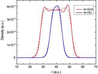
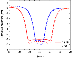
Figure 1: Ground state of two typical Na nanoshells containing $N=1919$ and $N=753$ electrons. Left panel: Electron densities computed using a DFT code (solid lines) and the fluid approach (dashed lines). Right panel: Effective potentials for the same cases. Reprinted with permission from Manfredi2018SPIE .

Before considering the dynamical response of the system, we need to compute its ground state. This can be obtained as a stationary solution of Eqs. (53)-(54) which is computed numerically using an iterative relaxation procedure Crouseilles2008 .

The electron density and effective potential profiles for two typical Na nanoshells containing respectively $N=1919$ and $N=753$ electrons are presented in Fig. 1. Both nanoshells have a central radius $R=40\,\rm a.u.$, but different thicknesses ($\Delta=10$ and $25\,\rm a.u.$). On the same figure, we also show the density profiles computed using a standard DFT code. The agreement is very good, and even more so considering that the fluid results (labeled QHD) require no more than a few minutes runtime on a standard desktop computer. In particular, the nonlocal spillout effect (electron density extending beyond the steplike ion density profile) is well described by the QHD method, even for the smaller structure ($N=753$), where the spillout is very prominent and the electron density is nowhere flat. For the larger nanoshell ($N=1919$), the two overdensities at the internal and external radii in the QHD density profile are a lower-order quantum effect, a remnant of the well-known Friedel oscillations visible in the corresponding DFT profile.

4.3 Numerical results: dynamics

Having computed the ground state of the electron system, we need to perturb it slightly in order to induce some dynamical behavior. As we are interested in plasmonic breathing modes, the perturbation will also be spherically symmetric. For the excitation, we use an instantaneous Coulomb potential applied at the initial time: $V_{ext}(r,t)=\frac{z}{r}\,\tau\,\delta(t),$ where $\delta$ is the Dirac delta function, $z$ is a fictitious charge quantifying the magnitude of the perturbation, and $\tau$ is the duration of the pulse.

In order to analyze the linear response of the system, we study the evolution of the mean radius of the electron cloud, defined as: $\langle r\rangle={1\over N}\int_{0}^{\infty}rn(r,t)\,4\pi r^{2}dr.$ The Fourier transform of $\langle r\rangle$ in the frequency domain is shown in Fig. 2, left frame. For the larger nanoshell ($N=1919$), the frequency spectrum shows a sharp peak near the plasmon frequency $\omega_{p}=\sqrt{3/r_{s}^{3}}=5.89$ eV. This behavior is compatible with the computed ground-state density profile (Fig. 1), which displays a region of almost constant density in between the inner and outer radii. In contrast, the spectrum of the smaller nanoshell ($N=753$) is much more fragmented and actually displays two principal peaks around the plasmon frequency, at about 5.6 eV and 6.2 eV, plus a number of smaller peaks at lower energies.

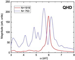
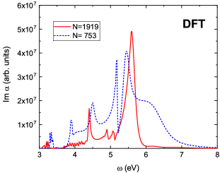
Figure 2: Linear-response frequency spectrum for two typical Na nanoshells containing $N=1919$ (red solid lines) and $N=753$ (blue dotted lines) electrons. Left frame: fluid (QHD) results; Right frame: TDDFT results. Reprinted with permission from Manfredi2018SPIE .

Still on Fig. 2 (right panel), we show the monopolar polarizability $\alpha$ computed with a linear-response TDDFT code Maurat2009 , using the same parameters and exchange-correlation functionals as for the fluid (QHD) simulations. The results compare rather favorably with the fluid ones. For $N=1919$, one dominant peak is observed at 5.6 eV, i.e. slightly redshifted compared to the pure plasmon frequency. This redshift can be understood in terms of dissipative phenomena (such as Landau damping, i.e. the coupling of the plasmon mode to single-particle modes) that are not included in the fluid description. More interestingly, the spectrum of the smaller nanoshell ($N=753$) reveals the same two-peak structure also observed in the fluid simulations, now with frequencies $\approx 5.16\,\rm eV$ and 5.45 eV, again slightly redshifted compared to corresponding peaks in the fluid spectrum. The more complex spectrum observed for $N=753$ is probably due to the shape of the ground state electron density, which looks more like a bell curve with no flat region inside the lattice jellium (see Fig. 1).

5 Fluid models with spin effects

The electrons are elementary fermions that carry not only an electric charge equal to $-e$, but also a magnetic moment (spin) equal to $\hbar/2$. The effect of the spin appears whenever the electron is immersed in a magnetic field. Even in the absence of an external field, an electron orbiting in the Coulomb potential of a positively-charged nucleus will feel the effect of a magnetic field in its own frame of reference (this “spin-orbit coupling” will be discussed in Sec. 5.4). Spin effects play an important role in many modern applications aimed at the storage and transfer of information, which go under the name of spintronics Hirohata2020 . In plasma physics, polarized electron beams can now be created and precisely manipulated in the laboratory Wu2019 ; Wu2020 ; Nie2021 ; Crouseilles2021 .

Some of the material presented in this section is taken from the PhD thesis of one of the co-authors Hurst2017phd .

5.1 General spin fluid equations

Fluid models that include spin effects are derived, as usual, from the corresponding kinetic (Wigner or Vlasov) equation by taking velocity moments. For spin-1/2 fermions, the Wigner function is no longer a scalar, but rather a $2\times 2$ matrix Arnold1989 . The fully quantum evolution equation of such matrix Wigner function is extremely complicated and hence of limited practical use. In the semiclassical limit, this equation gives rise to a matrix spin-Vlasov equation, which treats the electron motion in a classical fashion while preserving the intrinsically quantum character of the spin degrees of freedoms Hurst2014 ; Hurst2017 :

$$\frac{\partial f_{0}}{\partial t}+\bm{v}\cdot\bm{\nabla}f_{0}-\frac{e}{m}\left(\bm{E}+\bm{v}\times\bm{B}\right)\cdot\bm{\nabla_{v}}f_{0}+\frac{\mu_{B}}{2mc^{2}}\left(\bm{E}\times\bm{\nabla}\right)_{i}f_{i}$$

$$~{}-\frac{\mu_{B}}{m}\bm{\nabla}\left[B_{i}-\frac{1}{2c^{2}}\left(\bm{v}\times\bm{E}\right)_{i}\right]\cdot\bm{\nabla_{v}}f_{i}-\frac{\mu_{B}e}{2m^{2}c^{2}}\left[\bm{E}\times\left(\bm{B}\times\bm{\nabla_{v}}\right)\right]_{i}f_{i}=0.$$ (58)

$$\frac{\partial f_{i}}{\partial t}+\bm{v}\cdot\bm{\nabla}f_{i}-\frac{e}{m}\left(\bm{E}+\bm{v}\times\bm{B}\right)\cdot\bm{\nabla_{v}}f_{i}+\frac{\mu_{B}}{2mc^{2}}\left(\bm{E}\times\bm{\nabla}\right)_{i}f_{0}$$

$$~{}-\frac{\mu_{B}}{m}\bm{\nabla}\left[B_{i}-\frac{1}{2c^{2}}\left(\bm{v}\times\bm{E}\right)_{i}\right]\cdot\bm{\nabla_{v}}f_{0}-\frac{\mu_{B}e}{2m^{2}c^{2}}\left[\bm{E}\times\left(\bm{B}\times\bm{\nabla_{v}}\right)\right]_{i}f_{0}$$

$$~{}-\frac{2\mu_{B}}{\hbar}\left\{\left[\bm{B}-\frac{1}{2c^{2}}\left(\bm{v}\times\bm{E}\right)\right]\times\bm{f}\right\}_{i}=0,$$ (59)

where $(f_{0},\bm{f})$ are the four components of the $2\times 2$ matrix Wigner function, and $\bm{f}=(f_{x},f_{y},f_{z})$. The factor $\hbar$ is hidden in the definition of the Bohr magneton $\mu_{B}=e\hbar/(2m)$. The quantum corrections in Eqs. (58)- (59) (terms preceded by $\mu_{B}$) couple the orbital ($f_{0}$) and the spin ($f_{i}$) components of the Wigner function through the Zeeman effect and the spin-orbit interactions. The latter are given by those terms preceded by $1/c^{2}$, signalling that the spin-orbit coupling is a relativistic effect. There are no quantum corrections to the orbital electron dynamics because they appear only at the second order in $\hbar$.

Starting from the spin-Vlasov Eqs. (58) - (59), we derive the fluid equations by taking velocity moments of the phase-space distribution functions. At first, we will only include the Zeeman interaction. To obtain the fluid closure, we will employ a general procedure based on the maximization of entropy (see section 5.2). Fluid models with spin-orbit effects will be discussed further in section 5.4.

Going back to the Vlasov equations (58)-(59), we note that the scalar and vector distribution functions $f_{0}(\bm{r},\bm{v},t)$ and $\bm{f}(\bm{r},\bm{v},t)$ represent, respectively, the probability density for a particle to be at a point $(\bm{r},\bm{v})$ in the phase space and the probability density for that particle to have a spin directed along the direction of $\bm{f}$. Hence $f_{0}$ incorporates all the information unrelated to the spin, while $\bm{f}$ incorporates all information about the spin of the electron.

With these definitions, the particle density $n$ and the spin polarization $\bm{S}$ of the electron gas are easily expressed as moments of the distribution functions $f_{0}$ and $\bm{f}$:

$$n(\bm{r},t) = \int f_{0}(\bm{r},\bm{v},t)d\bm{v},$$ (60)

$$\bm{S}(\bm{r},t) = \frac{\hbar}{2}\int\bm{f}(\bm{r},\bm{v},t)d\bm{v}.$$ (61)

We further define the quantities

$$\bm{u} = \frac{1}{n}\int\bm{v}f_{0}d\bm{v},$$ (62)

$$J^{S}_{i\alpha} = \frac{\hbar}{2}\int v_{i}f_{\alpha}d\bm{v},$$ (63)

$$P_{ij} = m\int w_{i}w_{j}f_{0}d\bm{v},$$ (64)

$$\Pi_{ij\alpha} = \frac{\hbar}{2}m\int v_{i}v_{j}f_{\alpha}d\bm{v},$$ (65)

$$Q_{ijk} = m\int w_{i}w_{j}w_{k}f_{0}d\bm{v},$$ (66)

where we separated the mean fluid velocity $\bm{u}$ from the velocity fluctuations $\bm{w}\equiv\bm{v}-\bm{u}$. Here, $P_{ij}$ and $Q_{ijk}$ represent the pressure and the generalized energy flux tensors. They coincide with the corresponding definitions for spinless fluids with probability distribution function $f_{0}$. The spin-velocity tensor $J_{i\alpha}^{S}$ represents the mean fluid velocity along the $i$-th direction of the $\alpha$-th spin polarization vector, while $\Pi_{ij\alpha}$ represents the corresponding spin-pressure tensor. The evolution equations for the above fluid quantities are obtained by taking velocity moments of Eqs. (58) - (59):

$$\frac{\partial n}{\partial t}+\bm{\nabla}\cdot\left(n\bm{u}\right)=0,$$ (67)

$$\frac{\partial S_{\alpha}}{\partial t}+\partial_{i}J^{S}_{i\alpha}+\frac{e}{m}\left(\bm{S}\times\bm{B}\right)_{\alpha}=0,$$ (68)

$$\frac{\partial u_{i}}{\partial t}+u_{j}(\partial_{j}u_{i})+\frac{1}{nm}\partial_{j}P_{ij}+\frac{e}{m}\left[E_{i}+\left(\bm{u}\times\bm{B}\right)_{i}\right]+\frac{e}{nm^{2}}S_{\alpha}\left(\partial_{i}B_{\alpha}\right)=0,$$ (69)

$$\frac{\partial J^{S}_{i\alpha}}{\partial t}+\partial_{j}\Pi_{ij\alpha}+\frac{eE_{i}}{m}S_{\alpha}+\frac{e}{m}\epsilon_{jki}B_{k}J^{S}_{j\alpha}+\frac{e}{m}\epsilon_{jk\alpha}B_{k}J^{S}_{ij}+\frac{\mu_{B}\hbar}{2m}\left(\partial_{i}B_{\alpha}\right)n=0,$$ (70)

$$\frac{\partial P_{ij}}{\partial t}+u_{k}\partial_{k}P_{ij}+P_{jk}\partial_{k}u_{i}+P_{ik}\partial_{k}u_{j}+P_{ij}\partial_{k}u_{k}+\partial_{k}Q_{ijk}+\frac{e}{m}\big{[}\epsilon_{lki}B_{k}P_{jl}$$

$$\hskip 28.45274pt+\epsilon_{lkj}B_{k}P_{il}\big{]}+\frac{e}{m^{2}}\sum_{\alpha}\left[\partial_{i}B_{\alpha}\left(J^{S}_{j\alpha}-S_{\alpha}u_{j}\right)+\partial_{j}B_{\alpha}\left(J^{S}_{i\alpha}-S_{\alpha}u_{i}\right)\right]=0.$$ (71)

A different set of fluid equations for spin-1/2 particles was derived by Brodin and Marklund Brodin2007 using a Madelung transformation on the Pauli wave function. Another fluid theory was derived by Zamanian et al. Zamanian2010 from a Vlasov equation that includes the spin as an independent variable in an extended phase space Zamanian2010nj . More recently, a relativistic hydrodynamic model was obtained by Asenjo et al. Asenjo2011 from the Dirac equation. These approaches usually lead to cumbersome equations that are in practice very hard to solve, either analytically or numerically, even in the nonrelativistic limit.

Still another approach is based on a generalization of the Bloch equations Andreev2015 . Instead of adding “spin-dependent” moments to the usual ones as was done above – see Eqs. (61), (63), and (65) – Andreev Andreev2015 treats separately the spin-up and spin-down components in the corresponding Pauli equation. Performing a Madelung transformation for each component, one arrives at a set of four fluid equations (two continuity and two Euler equations), which are then closed using an appropriate equation of state for the pressure.

Going back to our fluid model (67)-(71), some further hypotheses are needed to close the set of equations. We first note that, by definition, the following equation is always satisfied: $\int w_{i}f_{0}d\bm{v}=0$. The same is not true, however, for the expression obtained by replacing $f_{0}$ with $f_{\alpha}$ in the preceding integral. If we assume that such a quantity indeed vanishes, i.e. $\int w_{i}f_{\alpha}d\bm{v}=0$, we immediately obtain that

$$J^{S}_{i\alpha}=u_{i}S_{\alpha}.$$ (72)

Physically, this means that the spin is simply transported along the average fluid velocity. This is of course an approximation that amounts to neglecting some spin-velocity correlations Zamanian2010 .

With this assumption, Eq. (70) is no longer necessary and the system of fluid equations reduces to

$$\frac{\partial n}{\partial t}+\bm{\nabla}\cdot\left(\bm{u}n\right)=0,$$ (73)

$$\frac{\partial S_{\alpha}}{\partial t}+\partial_{i}\left(u_{i}S_{\alpha}\right)+\frac{e}{m}\left(\bm{S}\times\bm{B}\right)_{\alpha}=0,$$ (74)

$$\frac{\partial u_{i}}{\partial t}+u_{j}(\partial_{j}u_{i})+\frac{1}{nm}\partial_{j}P_{ij}+\frac{e}{m}\left[E_{i}+\left(\bm{u}\times\bm{B}\right)_{i}\right]+\frac{e}{nm^{2}}S_{\alpha}\left(\partial_{i}B_{\alpha}\right)=0,$$ (75)

$$\frac{\partial P_{ij}}{\partial t}+u_{k}\partial_{k}P_{ij}+P_{jk}\partial_{k}u_{i}+P_{ik}\partial_{k}u_{j}+P_{ij}\partial_{k}u_{k}+\partial_{k}Q_{ijk}$$

$$\hskip 56.9055pt+\frac{e}{m}\big{[}\epsilon_{lki}B_{k}P_{jl}+\epsilon_{lkj}B_{k}P_{il}\big{]}=0.$$ (76)

Interestingly, in Eq. (74) the spin polarization is now transported by the fluid velocity $\mathbf{u}$, as in the model of Zamanian et al. Zamanian2010 . In order to complete the closure procedure, one can proceed in the same way as is usually done for spinless fluids, see section 2, for instance by assuming that the pressure is isotropic and replacing Eq. (76) with the polytropic expression (27).

5.2 Fluid closure: Maximum entropy principle

The maximum entropy principle (MEP) is a well-developed theory that has been successfully applied to various areas of gas, fluid, and solid-state physics Ali2012 ; Trovato2010 ; Romano2001 ; Anile1995 . The underlying assumption of the MEP is that, at equilibrium, the probability distribution function is given by the most probable microscopic distribution (i.e., the one that maximizes the entropy) compatible with some macroscopic constraints. The constraints are generally given by the various velocity moments, i.e., the local density, mean velocity, and temperature.

Here, we shall follow the derivation detailed in Hurst2014 . In order to illustrate the application of the MEP theory to a spin system, we write the Hamiltonian as follows

$$\mathcal{H}=m\frac{|\bm{v}|^{2}}{2}+V(\bm{r})\sigma_{0}+\mu_{B}\bm{B}\cdot\bm{\sigma},$$ (77)

where $\sigma_{0}$ is the $2\times 2$ identity matrix and $\bm{\sigma}$ is the vector of the Pauli matrices

$$\sigma_{x}=\begin{pmatrix}0&1\\ 1&0\end{pmatrix},\,\,\,\sigma_{y}=\begin{pmatrix}0&-i\\ i&0\end{pmatrix},\,\,\,\sigma_{z}=\begin{pmatrix}1&0\\ 0&-1\end{pmatrix}.$$ (78)

The relevant entropy density is

$$s(\mathcal{F})=\left\{\begin{array}[]{ll}k_{B}~{}Tr\left\{\mathcal{F}\log\mathcal{F}-\mathcal{F}\right\}&~{}~{}\textrm{(M--B)}\\[5.69054pt] k_{B}~{}Tr\left\{\mathcal{F}\log\mathcal{F}+(1-\mathcal{F})\log(1-\mathcal{F})\right\}&~{}~{}\textrm{(F--D),}\end{array}\right\},$$ (79)

for Maxwell-Boltzmann (M-B) and Fermi-Dirac (F-D) statistics, respectively. Here, $\mathcal{F}$ is the $2\times 2$ matrix Wigner function

$$\mathcal{F}=\frac{1}{2}\sigma_{0}f_{0}+\frac{1}{2}\bm{f}\cdot\bm{\sigma},$$ (80)

The detailed calculations for three- and four-moment closures are given in Hurst2014 . Here, we consider the simplest case where only three fluid moments (density $n$, mean velocity $\bm{u}$, and spin polarization $\bm{S}$) are kept,

For the M-B statistics, the pressure and the spin current at equilibrium turn out to be

$$P_{ij} = m{\rm Tr}\left(\int v_{i}v_{j}\mathcal{F}^{eq}d\bm{v}\right)-mnu^{2}=nk_{B}T\delta_{ij}$$ (81)

$$J^{S}_{i\alpha} = S_{\alpha}u_{i}.$$ (82)

Thus, considering three fluid moments and M-B statistics, leads to the standard expression for the isotropic pressure of an ideal gas, together with the “intuitive” closure condition (72) for the spin current tensor.

We repeated the above procedure for the F-D statistics and, as in the case of M-B, we recover the closure: $J^{S}_{i\alpha}=u_{i}S_{\alpha}$. For the pressure, we obtain

$$P = \frac{\hbar^{2}}{5m}\frac{\left(6\pi^{2}\right)^{2/3}}{2^{5/3}}\left[\left(n-\frac{2}{\hbar}|\bm{S}|\right)^{5/3}+\left(n+\frac{2}{\hbar}|\bm{S}|\right)^{5/3}\right].$$ (83)

When the spin polarization vanishes, Eq. (83) reduces to the usual expression of the zero-temperature pressure of a spinless Fermi gas (15). This can be interpreted as the total pressure of a plasma composed by two populations (spin-up and spin-down electrons). Due to the Zeeman splitting, the density of the particles whose spin is parallel to the magnetic field is lower than the energy of the particles whose spin is antiparallel. Equation (83) shows that the two populations provide a separate contribution to the total fluid pressure.

5.3 Linear dispersion relation

We want to compute the effect of the spin dynamics on the linear dispersion relation for Langmuir waves. To describe the electron dynamics, we use the following fluid model:

$$\frac{\partial n}{\partial t}+\bm{\nabla}\cdot\left(n\bm{u}\right)=0,$$ (84)

$$\frac{\partial S_{\alpha}}{\partial t}+\partial_{i}\left(u_{i}S_{\alpha}\right)+\frac{e}{m}\left(\bm{S}\times\bm{B}\right)_{\alpha}=0,$$ (85)

$$\frac{\partial u_{i}}{\partial t}+u_{j}\left(\partial_{j}u_{i}\right)+\frac{\partial_{i}P}{nm}+\frac{1}{m}\partial_{i}\left(-eV_{H}+V_{xc}\right)+\frac{e}{nm^{2}}S_{\alpha}\partial_{i}\left(\bm{B}+\bm{B_{xc}}\right)_{\alpha},$$ (86)

where we have used the closure relations: $J^{S}_{i\alpha}=u_{i}S^{\alpha}$ for the spin current, and $P=n_{0}k_{B}T(n/n_{0})^{\gamma}$ for the isotropic pressure. The Hartree potential is a solution of Poisson’s equation: $\bm{\nabla}^{2}V_{H}=\frac{e}{\epsilon_{0}}(n-n_{0})$, where $n_{0}$ is the homogeneous ion density.

The above equations are essentially identical to Eqs. (73)-(75), with some extra terms:

1. The magnetic field $\bm{B}(\bm{r},t)=\bm{\nabla}\times\bm{A}(\bm{r},t)$ is a solution of the quasi-static Maxwell-Ampère equation

   $$\bm{\nabla}^{2}\bm{A}(\bm{r},t)=-\frac{e}{m}\mu_{0}\bm{\nabla}\times\bm{S}(\bm{r},t).$$ (87)

   Note that we did not consider the self-consistent magnetic field created by charge currents and neglected the Lorentz force in the momentum equation (86). The reason is that we focus on plasma waves propagating in a well-defined longitudinal axis, with no coupling to the other transverse directions. Hence, the only contribution to the magnetic field arises from the spin polarization $\bm{S}$ and accounts for magnetic dipole interactions.

2. We include the exchange and correlation fields $V_{xc}[n(\bm{r},t),\bm{m}(\bm{r},t)]$ and $\bm{B}_{xc}[n(\bm{r},t),\bm{m}(\bm{r},t)]$. Here, $\bm{m}=2\bm{S}/\hbar$ is the magnetization vector, which has the same dimensions as the electron density and can be used to compute the electron polarization rate: $\eta=|\bm{m}|/n$. Exchange and correlation potentials can be taken from the vast literature on DFT (see, for instance Maurat2009 Gunnarsson1976 ) and enable us to go beyond the mean-field approximation, where the only electron-electron interactions are those modeled by the self-consistent Hartree potential. For the present derivation, it is not necessary to provide an explicit form for the exchange and correlation fields.

To obtain the dispersion relation of plasma oscillations, we study the evolution of a small deviations from the equilibrium. The equilibrium state is given by a homogeneous electron gas with density $n_{0}$ and vanishing mean velocity ($u_{0}=0$), which is initially spin-polarized along the $z$ direction ($\bm{S}=S_{0}\hat{e}_{z}$). Assuming that the perturbations are plane waves propagating in the $x$ direction, we can express the fluid quantities as follows:

$$n(\bm{r},t) =n_{0}+\delta n\exp\left[i\left(kx-\omega t\right)\right],$$ (88)

$$\bm{S}(\bm{r},t) =\bm{S}_{0}+\bm{\delta S}\exp\left[i\left(kx-\omega t\right)\right],$$ (89)

$$\bm{u}(\bm{r},t) =\bm{\delta u}\exp\left[i\left(kx-\omega t\right)\right],$$ (90)

where the subscript $0$ denotes quantities at equilibrium and the $\delta$ quantities are small perturbations. We write the self-consistent and the exchange-correlation fields in the same way as

$$\phi(\bm{r},t) =\delta\phi\exp\left[i\left(kx-\omega t\right)\right],$$ (91)

$$\bm{B}(\bm{r},t) =\bm{\delta B}\exp\left[i\left(kx-\omega t\right)\right],$$ (92)

$$V_{xc}[n,\bm{m}] =V_{xc}[n_{0},\bm{m_{0}}]+\left(\delta n\left.\frac{\partial V_{xc}}{\partial n}\right|_{\underset{\bm{m_{0}}}{n_{0}}}+\frac{2}{\hbar}\bm{\delta S}\cdot\left.\frac{\partial V_{xc}}{\partial\bm{m}}\right|_{\underset{\bm{m_{0}}}{n_{0}}}\right)e^{i(kx-\omega t)},$$ (93)

$$B_{xc}[n,\bm{m}] =B_{xc}[n_{0},\bm{m_{0}}]+\left(\delta n\left.\frac{\partial B_{xc}}{\partial n}\right|_{\underset{\bm{m_{0}}}{n_{0}}}+\frac{2}{\hbar}\bm{\delta S}\cdot\left.\frac{\partial B_{xc}}{\partial\bm{m}}\right|_{\underset{\bm{m_{0}}}{n_{0}}}\right)e^{i(kx-\omega t)}.$$ (94)

Injecting Eqs. (88)-(94) into the fluid equations (84)-(86) and retaining only first-order terms yields the following dispersion relation:

$$\omega^{2} =\omega_{p}^{2}+k^{2}\gamma\frac{k_{B}T}{m}+$$

$$k^{2}\frac{n_{0}}{m}\left(\frac{\partial V_{xc}}{\partial n}+\eta_{0}\frac{\partial V_{xc}}{\partial m_{z}}+\eta_{0}\mu_{B}\frac{\partial B_{xc}}{\partial n}+\eta_{0}^{2}\mu_{B}\frac{\partial B_{xc}}{\partial m_{z}}\right)-k^{2}\frac{\mu_{B}^{2}\mu_{0}n_{0}}{m}\eta_{0}^{2},$$ (95)

where $\eta_{0}=|\bm{m}_{0}|/n_{0}$ is the equilibrium polarization. The second term on the right-hand side is the usual thermal correction (Bohm-Gross), the next term represents the exchange-correlation corrections, and the last term derives from the self-consistent magnetic field [Maxwell-Ampère equation (87)]. Terms preceded by $\eta_{0}$ are due to the electron polarization

The above dispersion relation (95) is identical (in the small wave number $k$ regime) to that obtained from the corresponding spin-Vlasov equations in Manfredi2019 (see section 7.3), provided that the polytropic exponent is taken $\gamma=3$, as was discussed earlier in section 3.2.

5.4 Spin-orbit coupling

In the above calculations, we constructed fluids models with spin effects by only considering the Zeeman interaction. The same procedure can be carried over to the case where spin-orbit interactions are included Hurst2017 . A straightforward integration of Eqs. (58)-(59), with respect to the velocity variable, leads to the following fluid equations :

$$\frac{\partial n}{\partial t}+\bm{\nabla}\cdot\left(n\bm{\overline{u}}\right)=0,$$ (96)

$$\frac{\partial S_{\alpha}}{\partial t}+\partial_{i}\overline{J}^{S}_{i\alpha}+\frac{e}{m}\left(\bm{S}\times\bm{B}\right)_{\alpha}+\frac{e}{2mc^{2}}\epsilon_{jk\alpha}\epsilon_{rlj}E_{l}J^{S}_{rk}=0,$$ (97)

$$\frac{\partial u_{i}}{\partial t}+u_{j}(\partial_{j}u_{i})+\frac{1}{nm}\partial_{j}P_{ij}+\frac{e}{m}\left[E_{i}+\left(\bm{\widetilde{u}}\times\bm{B}\right)_{i}\right]+\frac{e}{nm^{2}}S_{\alpha}\left(\partial_{i}B_{\alpha}\right)$$

$$~{}+\frac{\mu_{B}}{2mc^{2}n}\epsilon_{jkl}\left[u_{i}\partial_{j}\left(E_{k}S_{l}\right)+E_{j}\left(\partial_{k}J^{S}_{il}\right)-\left(\partial_{i}E_{k}\right)J^{S}_{jl}-\left(\partial_{j}E_{k}\right)J^{S}_{il}\right]=0,$$ (98)

$$\frac{\partial J^{S}_{i\alpha}}{\partial t}+\partial_{j}\Pi_{ij\alpha}+\frac{eE_{i}}{m}S_{\alpha}+\frac{e}{m}\epsilon_{jki}B_{k}\widetilde{J}^{S}_{j\alpha}+\frac{e}{m}\epsilon_{jk\alpha}B_{k}J^{S}_{ij}+\frac{\mu_{B}\hbar}{2m}\left(\partial_{i}B_{\alpha}\right)n$$

$$~{}+\frac{\mu_{B}}{2mc^{2}}\epsilon_{kl\alpha}\partial_{l}\left(E_{k}nu_{i}\right)-\frac{\mu_{B}}{2mc^{2}}\epsilon_{kl\alpha}\left(\partial_{i}E_{l}\right)nu_{k}+\frac{\mu_{B}}{\hbar c^{2}}\epsilon_{kl\alpha}\epsilon_{rsk}E_{s}\Pi^{S}_{irl}=0,$$ (99)

$$\frac{\partial P_{ij}}{\partial t}+u_{k}\partial_{k}P_{ij}+P_{jk}\partial_{k}u_{i}+P_{ik}\partial_{k}u_{j}+P_{ij}\partial_{k}u_{k}+\partial_{k}Q_{ijk}+\frac{e}{m}\left[\epsilon_{kli}P_{jk}+\epsilon_{klj}P_{ik}\right]B_{l}$$

$$~{}+\frac{\mu_{B}}{m}\left[\partial_{i}B_{k}\left(J^{S}_{jk}-u_{j}S_{k}\right)+\partial_{j}B_{k}\left(J^{S}_{ik}-U_{i}S_{k}\right)\right]+\frac{\mu_{B}}{2mc^{2}}\epsilon_{rsl}\partial_{s}\left[E_{r}\left(\Pi^{S}_{ijl}-u_{i}u_{j}S_{l}\right)\right]$$

$$~{}+\frac{\mu_{B}}{2mc^{2}}\epsilon_{rkp}E_{r}\left[\epsilon_{kli}\left(J^{S}_{jp}-u_{j}S_{p}\right)+\epsilon_{klj}\left(J^{S}_{ip}-u_{i}S_{p}\right)\right]B_{l}$$

$$~{}-\frac{\mu_{B}}{2mc^{2}}\epsilon_{rsl}\left[\partial_{i}E_{s}\left(\Pi^{S}_{jrl}-u_{j}J^{S}_{rl}\right)+\partial_{j}E_{s}\left(\Pi^{S}_{irl}-u_{i}J^{S}_{rl}\right)\right]$$

$$~{}-\frac{\mu_{B}}{2mc^{2}}u_{i}\epsilon_{rsl}\partial_{s}\left[E_{r}\left(J^{S}_{jl}-u_{j}S_{l}\right)\right]-\frac{\mu_{B}}{2mc^{2}}u_{j}\epsilon_{rsl}\partial_{s}\left[E_{r}\left(J^{S}_{il}-u_{i}S_{l}\right)\right]=0,$$ (100)

where we introduced a new average velocity and a new spin current

$$\overline{\bm{u}}=\bm{u}-\frac{\mu_{B}}{2mc^{2}n}\bm{E}\times\bm{S},~{}~{}~{}~{}\overline{J}^{S}_{ij}=J^{S}_{ij}+\frac{\mu_{B}}{2mc^{2}}\epsilon_{ijk}E_{k}n.$$ (101)

Some further hypotheses are needed to close the above set of equations (96)-(100). Inspecting the evolution equation (100) for the pressure tensor, one notices that most spin-dependent terms cancel if we set

$$J^{S}_{i\alpha}=u_{i}S_{\alpha}~{}~{}~{}~{}\textrm{and}~{}~{}~{}~{}\Pi^{S}_{ij\alpha}=u_{i}J^{S}_{j\alpha}.$$ (102)

This is a generalization of the simple closure described in section 5, whereby both the spin density $S_{\alpha}$ and the spin current $J^{S}_{j\alpha}$ are transported by the mean fluid velocity $u_{i}$.

With this assumption, Eq. (99) and the definition of the spin-pressure $\Pi_{ij\alpha}$ are no longer necessary. The system of fluid equations simplifies to

$$\frac{\partial n}{\partial t}+\bm{\nabla}\cdot\left(n\bm{\overline{u}}\right)=0,$$ (103)

$$\frac{\partial S_{\alpha}}{\partial t}+\partial_{i}\left(u_{i}S_{\alpha}\right)-\frac{\mu_{B}}{2mc^{2}}\left(\bm{\nabla}\times n\bm{E}\right)_{\alpha}+\frac{e}{m}\left[\bm{S}\times\left(\bm{B}-\frac{1}{2c^{2}}\bm{u}\times\bm{E}\right)\right]_{\alpha}=0,$$ (104)

$$\frac{\partial u_{i}}{\partial t}+u_{j}(\partial_{j}u_{i})+\frac{1}{nm}\partial_{j}P_{ij}+\frac{e}{m}\left[E_{i}+\left(\bm{\overline{u}}\times\bm{B}\right)_{i}\right]+\frac{e}{nm^{2}}S_{\alpha}\left(\partial_{i}B_{\alpha}\right)$$

$$~{}+\frac{\mu_{B}}{2mc^{2}n}\epsilon_{jkl}\left[E_{j}\left(\partial_{k}u_{i}\right)-u_{k}\left(\partial_{i}E_{j}\right)\right]S_{l}=0,$$ (105)

$$\frac{\partial P_{ij}}{\partial t}+u_{k}\partial_{k}P_{ij}+P_{jk}\partial_{k}u_{i}+P_{ik}\partial_{k}u_{j}+P_{ij}\partial_{k}u_{k}+\partial_{k}Q_{ijk}+\frac{e}{m}\left[\epsilon_{kli}P_{jk}+\epsilon_{klj}P_{ik}\right]B_{l}=0.$$ (106)

Then, by supposing that the system is isotropic and adiabatic, i.e. $P_{ij}\propto n^{\frac{d+2}{d}}\delta_{ij}$ (where $d$ is the number of degrees of freedom) and $Q_{ijk}=0$, one is able to close the system of fluid equation.

In summary, Eqs. (103)-(105), together with an adapted expression of the pressure, constitute a closed system of hydrodynamic equations including spin-orbit effects.

6 Variational approach to the quantum fluid models

6.1 Basics: Lagrangian formulation of the fluid equations

We recall the quantum fluid equations considered in section 2, written here in atomic units ($4\pi\varepsilon_{0}=e=\hbar=1$):

$$\frac{\partial n}{\partial t}+\bm{\bm{\nabla}}\!\cdot(n\bm{u})=0,$$ (107)

$$\frac{\partial\bm{u}}{\partial t}+\bm{u}\cdot\!\bm{\bm{\nabla}}\bm{u}=\bm{\bm{\nabla}}\!\,V_{H}+\bm{\bm{\nabla}}\!\,V_{ext}-\frac{\bm{\bm{\nabla}}P}{n}+\frac{1}{2}\bm{\bm{\nabla}}\left(\frac{\bm{\bm{\nabla}}^{2}\sqrt{n}}{\sqrt{n}}\right),$$ (108)

$$\bm{\bm{\nabla}}^{2}V_{H}=4\pi n,$$ (109)

with the degenerate pressure $P={1\over 5}\left(3\pi^{2}\right)^{2/3}n^{5/3}.$

The above fluid equations may be represented by a Lagrangian density $\mathscr{L}(n,\theta,V_{H})$, where $\theta(\bm{r},t)$ is related to the velocity through $\bm{u}=\bm{\nabla}\theta$. The expression of such Lagrangian density reads as:

$$\mathscr{L}(n,\theta,V_{H}) =\frac{n}{2}\left(\bm{\bm{\nabla}}\theta\right)^{2}+n\frac{\partial\theta}{\partial t}+\frac{1}{8n}\left(\bm{\bm{\nabla}}n\right)^{2}+\frac{3}{10}\left(3\pi^{2}\right)^{2/3}n^{5/3}$$

$$~{}-nV_{ext}-nV_{H}-\frac{1}{8\pi}\left(\bm{\bm{\nabla}}V_{H}\right)^{2}.$$ (110)

By taking the Euler-Lagrange equations with respect to the three fields $\chi_{i}=\{n,\theta,V_{H}\}$

$$\frac{\partial\mathscr{L}}{\partial\chi_{i}}-\nabla\cdot\frac{\partial\mathscr{L}}{\partial\nabla\chi_{i}}-\frac{\partial}{\partial t}\frac{\partial\mathscr{L}}{\partial\dot{\chi}_{i}}=0,$$ (111)

one recovers exactly the quantum fluid equations (107)-(109).

So far, no approximations were made. In order to derive a tractable system of equations, one needs to specify a particular ansatz for the electron density. In general, we posit that the density depends on the position $\bm{r}$ and, parametrically, on $N$ functions of time $d_{1}(t),\cdots,d_{N}(t)$, which are not specified for the moment. Hence we write:

$$n(\bm{r},t)={\cal N}\left[\bm{r};d_{1}(t),d_{2}(t),\cdots,d_{N}(t)\right].$$ (112)

With this assumption, the time dependence of the electronic density is embedded in the dynamical variables $d_{1}(t),\cdots,d_{N}(t)$. The spatial profile ${\cal N}$ of the density can, for instance, be tuned to match the ground state of the system.

The reduced Lagrangian $L$ is obtained by integrating the Lagrangian density over all space

$$L\left(\{d_{i}(t)\},\{\dot{d}_{i}(t)\}\right)=\int\mathscr{L}\left(\bm{r},\{d_{i}(t)\},\{\dot{d}_{i}(t)\}\right)d\bm{r}.$$ (113)

Then, the Lagrangian $L$ can be used to find the dynamical equations for the parameters $d_{i}(t)$ through the Euler-Lagrange equations:

$$\frac{\partial L}{\partial d_{i}}-\frac{\textrm{d}}{\textrm{d}t}\frac{\partial L}{\partial\dot{d}_{i}}=0,$$ (114)

which yield a system of differential equations such as

$$\left\{\begin{array}[]{ccc}\ddot{d}_{1}(t)&=&f_{1}\left(d_{1}(t),\cdots,d_{N}(t)\right),\\ \ddot{d}_{2}(t)&=&f_{2}\left(d_{1}(t),\cdots,d_{N}(t)\right),\\ \vdots&&\\ \ddot{d}_{N}(t)&=&f_{N}\left(d_{1}(t),\cdots,d_{N}(t)\right).\end{array}\right.$$ (119)

In summary, thanks to the above variational approach, the very complex nonlinear many-body dynamics has been translated into a set of ordinary differential equations for the quantities $d_{i}(t)$. The latter may be easily solved with standard numerical methods, such as Runge-Kutta.

For practical applications, the variational method can be difficult to use. Indeed, to find the Lagrangian (113) one has to specify, in addition to the electron density, an analytical expression for the fields $\theta(\bm{r},t)$ and $V_{H}(\bm{r},t)$ as functions of the dynamical variables. The field $\theta(\bm{r},t)$ is related to the mean velocity and should satisfy the continuity equation (107), while the field $V_{H}$ has to obey Poisson’s equation (109). It is worth insisting on the fact that we need to find analytical expressions of $\theta$ and $V_{H}$ to make the variational approach useful for applications. However, this can be difficult to do in practice and depends mostly on the mathematical expression that we assumed for the electronic density, i.e. on the function ${\cal N}$ in Eq. (112). Nevertheless, the procedure generally yields rather robust results. For instance, it was noted in Haas2009 that, even for an approximate density profile, the resonant frequencies computed with the variational method are still very close to the exact ones, as will be shown in the forthcoming subsection.

6.2 Application I: Electronic breathing mode in a 1D quantum well

As an example of application of the variational method, we consider an electron gas trapped in a 1D harmonic potential . This is a situation that can be encountered when modeling the electron dynamics in a semiconductor quantum well. The evolution of the electron density $n(x,t)$ and mean velocity $u(x,t)$ is governed by the following 1D continuity and momentum equations

$$\frac{\partial n}{\partial t} + \frac{\partial}{\partial x}\,(nu)=0\,,$$ (120)

$$\frac{\partial\,u}{\partial\,t} + u\frac{\partial u}{\partial x}=-\frac{1}{mn}\frac{\partial P}{\partial x}-\frac{1}{m}\frac{\partial V}{\partial x}+\frac{\hbar^{2}}{2m^{2}}~{}\frac{\partial}{\partial x}\left(\frac{\partial_{x}^{2}\sqrt{n}}{\sqrt{n}}\right),$$ (121)

where $m$ is the effective electron mass, $\hbar$ is the reduced Planck constant, $P(x,t)$ is the electron pressure, and $V=V_{\rm conf}(x)+V_{H}(x,t)$ is the effective potential, which is composed of a confining and a Hartree term. The Hartree potential obeys the Poisson equation, namely $V_{H}^{\prime\prime}=-e^{2}\,n/\varepsilon$, where $\varepsilon$ is the effective dielectric permittivity of the material.

The pressure $P(x,t)$ in Eq. (121) is related to the electron density $n$ via a polytropic equation of state: $P=\overline{n}\,k_{B}\,T\,(n/\overline{n})^{\gamma}$, where $\gamma=3$ is the 1D polytropic exponent and $\overline{n}$ is the mean electron density.

The electrons are confined by a harmonic potential $V_{\rm conf}=\frac{1}{2}\omega_{0}^{2}mx^{2}$, where $\omega_{0}$ can be related to a fictitious homogeneous positive charge of density $n_{0}$ via the relation $\omega_{0}=(e^{2}n_{0}/m\epsilon)^{1/2}$. We then normalize time to $\omega_{0}^{-1}$; space to $\lambda_{0}=(k_{B}\,T/m)^{1/2}/\omega_{0}$; velocity to $\lambda_{0}\,\omega_{0}$; energy to $k_{B}T$; and the electron density to $n_{0}$. Quantum effects are encapsulated in the scaled Planck constant $H=\hbar\,\omega_{0}/k_{B}\,T$. These nondimensional units will be used in the rest of this section.

The system of Eqs. (120)–(121) corresponds to the following Lagrangian density:

$${\cal L}(n,\theta,V_{H}) = \frac{1}{2}\left(\frac{\partial V_{H}}{\partial x}\right)^{2}-n\,V_{H}-\,n\,\frac{\partial\theta}{\partial t}-\int^{n}W(n^{\prime})\,dn^{\prime}$$ (122)

$$- \frac{1}{2}\,\left(n\,\left[\frac{\partial\theta}{\partial x}\right]^{2}+\frac{H^{2}}{4n}\,\left[\frac{\partial\,n}{\partial x}\right]^{2}\right)-n\,V_{\rm conf}\,.$$

The velocity field can be written as the gradient of the ancillary function $\theta(x,t)$, as $u=\partial\theta/\partial x$. The potential $W(n)$ in Eq. (122) is a function of the pressure, $W\equiv\int^{n}\frac{dP}{dn^{\prime}}\frac{dn^{\prime}}{n^{\prime}}=(3/2)(n/\overline{n})^{2}$. The Euler-Lagrange equations with respect to $n$, $\theta$ and $V_{H}$ yield the equations of motion (120)–(121), as well as the Poisson equation for $V_{H}$.

We further assume a Gaussian profile for the electron density

$$n(x,t)=\frac{A}{\sigma}\,\exp\left[-\frac{(x-d\,)^{2}}{2\,\sigma^{2}}\right]\,,$$ (123)

where $d(t)$ and $\sigma(t)$ are time-dependent functions that represent the center-of-mass (dipole) and the spatial dispersion of the electron gas, respectively. The constant $A=N/\sqrt{2\pi}$, is defined in terms of the total number of electrons $N=\int n\,dx$.

The other fields to be inserted in the Lagrangian (122) are $\theta$ and $V_{H}$ and they are determined by requiring that the continuity and Poisson equations are satisfied. Inserting the Ansatz of Eq. (123) into the continuity equation (120), one obtains: $\theta=(\dot{\sigma}/2\sigma)(x-d)^{2}+\dot{d}(x-d)$. The solution of the Poisson equation with a Gaussian electron density is

$$V_{H}=-A\,\sigma\,e^{-\xi^{2}/2\sigma^{2}}-A\,\sqrt{\frac{\pi}{2}}\,\xi\,{\rm Erf}\left(\frac{\xi}{\sqrt{2}\,\sigma}\right)+\rm const,$$ (124)

where ${\rm Erf}$ is the error function.

Finally, one obtains the Lagrangian

$$L = \frac{1}{\sqrt{2\pi}\,A}\,\int\,{\cal L}\,dx=\frac{\dot{d}^{2}+{\dot{\sigma}}^{2}}{2}-\frac{d^{2}+\sigma^{2}}{2}$$ (125)

$$+ \frac{\sqrt{2}}{2}\,A\,\sigma-\,\frac{\sqrt{3}\,A^{2}}{6\,\overline{n}^{2}\,\sigma^{2}}-\frac{H^{2}}{8\,\sigma^{2}}\,,$$

which only depends on the dipole $d$ and the variance $\sigma$ and their time derivatives. The Euler-Lagrange equations corresponding to the Lagrangian $L$ read as

$$\ddot{d} + d=0,$$ (126)

$$\ddot{\sigma} + \sigma=\frac{\sqrt{2}\,A}{2}+\frac{\sqrt{3}\,A^{2}}{3\,\overline{n}^{2}\,\sigma^{3}}+\frac{H^{2}}{4\,\sigma^{3}}\,.$$ (127)

The confining potential $V_{\rm conf}$ appears in the harmonic forces on the left-hand side of Eqs. (126) and (127). It should be noted that the equations for $d$ and $\sigma$ decouple for purely harmonic confinement. Equation (126) describes rigid oscillations of the electron gas at the effective plasmonic frequency, the so-called Kohn mode Kohn1961 . Equation (127) describes the dynamics of the breathing mode, i.e. coherent oscillations of the width of the electron density around an equilibrium value given by $\ddot{\sigma}=0$. The three terms on the right-hand side of Eq. (127) represent respectively the Coulomb repulsion, the electron pressure, and the Bohm potential.

Figure 3: The breather frequency $\Omega$ as a function of $A$, for $H=0.5$. Solid line: analytical results from the variational method. Squares: The Wigner-Poisson simulations. The inset shows the mean electron density $\langle n\rangle$ as a function of $A$. Reprinted with permission from Haas2009 . Copyright (2009) by the American Physical Society.

The frequency $\Omega=\Omega(A,H)$ of the breathing mode can be obtained by linearizing the equation of motion (127) in the vicinity of the stable fixed point of $U(\sigma)$. The behavior of the breathing frequency with $A$ (which is proportional to the electron density) is shown in Fig. 3. For $A=0$ (i.e., when the Coulomb interaction is switched off) the exact frequency is $\Omega=2\omega_{0}$. For finite $A$, the breathing frequency decreases and approaches $\Omega=\omega_{0}$, for $A\to\infty$. This is due to the fact that, for large $A$, the electron density becomes flat and equal to $n_{0}$ (see the inset of Fig. 3), and is exactly neutralized by the ion density background. For such a spatially homogeneous system, one can use the results of the Bohm-Gross dispersion relation, which yields $\Omega=\omega_{0}$ for long wavelengths.

The above analytical results were compared to numerical simulations of the full Wigner-Poisson equations. The results of the simulations, also plotted in Fig. 3, agree very well with the theoretical curve based on the Lagrangian approach. The agreement slightly deteriorates for larger values of $A$, because the electron density deviates from the Gaussian profile due to strong Coulomb repulsion.

In summary, the variational method described here enabled us to obtain analytically the frequency of the breathing mode oscillations in the linear regime, with excellent agreement in comparison with “exact” Wigner-Poisson simulations. Nevertheless, the method is not restricted to the linear response and can be used for large perturbations as well. The only requirement is that the density ansatz (123) is approximately verified.

6.3 Application II: Chaotic electron motion in a 3D nonparabolic anisotropic well

The same approach was later extended to the case of nonparabolic and anisotropic wells Hurst2016 . The confining potential is the sum of a harmonic and an anharmonic (but isotropic) part:

$$V_{\text{conf}}=\frac{1}{2}\left(k_{x}x^{2}+k_{y}y^{2}+k_{z}z^{2}\right)+\zeta\left(x^{2}+y^{2}+z^{2}\right)^{2},$$ (128)

where $k_{i}>0$ is the stiffness in the $i$-th direction and $\zeta\geq 0$ measures the relative strength of the anharmonic part of the potential.

The algebra is much more convoluted than in the preceding 1D case, but it is still possible to obtain a Lagrangian function $L$ that depends on the six variables $\{d_{i}(t),\sigma_{i}(t)\}$ and their time derivatives, where $i=x,y,z$ denotes the Cartesian axes:

$$L[d_{i},\sigma_{i},\dot{d}_{i},\dot{\sigma}_{i}]=\frac{1}{N}\int\mathcal{L}d\bm{r}=\frac{1}{2}\sum_{i}\left(\dot{\sigma_{i}}^{2}+\dot{d_{i}}^{2}\right)-U(d_{i},\sigma_{i}),$$ (129)

where $N$ is the total number of electrons and $U(d_{i},\sigma_{i})=U_{d}(d_{i})+U_{\sigma}(\sigma_{i})+U_{d\sigma}(d_{i},\sigma_{i})$. The different potential terms read as:

$$U_{d}= \frac{1}{2}\sum_{i}k_{i}d_{i}^{2},$$ (130)

$$U_{\sigma}= \frac{1}{2}\sum_{i}k_{i}\sigma_{i}^{2}+\left(\sum_{i}\frac{1}{\sigma_{i}^{2}}\right)\left(\frac{1}{8}+\alpha_{1}N\big{[}\sigma_{x}\sigma_{y}\sigma_{z}\big{]}^{1/3}\!-\,\alpha_{2}\,\beta\bigg{[}\frac{\sigma_{x}\sigma_{y}\sigma_{z}}{N}\bigg{]}^{1/3}\right)$$

$$+\,\alpha_{3}\bigg{[}\frac{N}{\sigma_{x}\sigma_{y}\sigma_{z}}\bigg{]}^{2/3}\!\!-\,\alpha_{4}\bigg{[}\frac{N}{\sigma_{x}\sigma_{y}\sigma_{z}}\bigg{]}^{1/3},$$ (131)

$$U_{d\sigma}= \zeta\Bigg{[}\sum_{i}\Big{(}3\hskip 0.85358pt\sigma_{i}^{4}+6\hskip 0.85358ptd_{i}^{2}\sigma_{i}^{2}+d_{i}^{4}\Big{)}\,+\sum_{i\neq k}\!\!\Big{(}\sigma_{i}^{2}+d_{i}^{2}\Big{)}\Big{(}\sigma_{k}^{2}+d_{k}^{2}\Big{)}\Bigg{]},$$ (132)

and represent respectively the dipole motion ($U_{d}$), the breathing motion ($U_{\sigma}$), and the coupling between the dipole and breathing dynamics ($U_{d\sigma}$). Note that such coupling disappears for purely harmonic confinement ($\zeta=0$). The $\alpha_{j}$ are dimensionless coefficients. The equations of motion obtained from the Euler-Lagrange equations read as:

$$\ddot{d_{i}}=-\frac{\partial U_{d}}{\partial d_{i}}-\frac{\partial U_{d\sigma}}{\partial d_{i}},~{}~{}~{}~{}~{}\ddot{\sigma_{i}}=-\frac{\partial U_{\sigma}}{\partial\sigma_{i}}-\frac{\partial U_{d\sigma}}{\partial\sigma_{i}}.$$ (133)

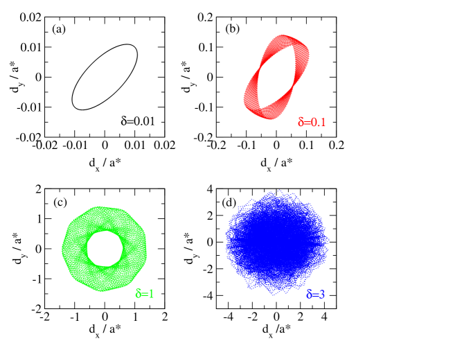
Figure 4: Poincaré sections in the plane $(d_{x},d_{y})$ for different values of the initial excitation: $\delta=0.01$ (a), 0.1 (b), 1 (c), and 3 (d). The simulations were performed for an anisotropic well with $k_{x}=k_{y}=5$, $k_{z}=1$, $N=50$, and $\zeta=0.01$; $a^{\displaystyle*}$ is a reference length. Reprinted with permission from Hurst2016 . Copyright (2016) by the American Physical Society.

Figure 4 shows the Poincaré maps in the $(d_{x},d_{y})$ plane for increasing values of the initial excitation $\delta$ [$d_{i}=\delta$, $\dot{d}_{x}=-\dot{d}_{y}=\delta$ and $\dot{d}_{z}=0$, at $t=0$]. At low excitation, the motion is periodic. When $\delta$ is increased, the phase space area progressively fills up, first in a regular way (up to $\delta=1$), and then in an irregular ergodic way. The latter behavior clearly indicates the presence of chaotic motion.

7 Conclusions and perspectives

The aim of this short review was to present the results on quantum fluid models obtained in our research group at the University of Strasbourg during the last two decades. We covered the basics of quantum fluid models for systems of spinless particles, then extended the models to include the spin degrees of freedom, as well as semirelativistic corrections. In the last part, we outlined the bases of a variational approach which enables one to reduce the complexity of the fluid models to a set of simple ordinary differential equations for macroscopic quantities such as the center of mass and the width of the electron density. Several examples taken from past works illustrated the applications of quantum fluid theory to various physical systems, mainly issued from condensed matter and nanophysics. Other areas of possible interest for these methods include laser-plasma interactions Crouseilles2021 and warm dense matter Dornheim2018 ; Fourment2014 . Applications to the astrophysics of compact objects Uzdensky2014 were not addressed here, but are surely an important area for future research.

Some care was devoted to establish the validity of the quantum fluid models under consideration (see section 3). This was done by comparing the dispersion relations obtained from the fluid models to those derived from a fully kinetic mean-field approach (Vlasov or Wigner). We analyzed in particular the limiting cases of high-frequency (Langmuir) and low-frequency (acoustic) waves. Checking the validity and limits of applicability of the various quantum fluid models is an issue that is unfortunately often neglected in the literature Bonitz2019 , and we encourage future investigators on these topics to do so systematically.

From a fundamental point of view, the relationships of the quantum fluid methods to the time-dependent density functional theory (TDDFT) Moldabekov2018 ; Manfredi2019 and Thomas-Fermi theory Michta2015 were highlighted in several past works. Much less explored is the close link to the so-called orbital-free density functional theory Witt2018OFDFT , which appears to be closely related to the present fluid theory. More work is needed to clarify the similarities and differences between the two approaches.

Finally, some effort should be directed to generalize the quantum fluid models in order to include non-ideal effects, such as dynamical correlations that lead to dissipation and damping. These effects are important on timescales going beyond the electron coherence time, which for standard metallic nano-objects is of the order of 100 fs.

In nanophysics, estimating the viscosity of a quantum electron gas is an open and interesting problem, with applications to graphene and other low dimensional materials Levitov2016 .

There have been some attempts to include potentially dissipative effects in TDDFT. The most accomplished of such attempts is the so-called time-dependent current-density-functional theory developed by Vignale and Kohn Vignale97 , which uses the electron current density $\bm{j}(\bm{r},t)$ as the basic building block, instead of the density $n(\bm{r},t)$. However, the relevant equations are mathematically very complicated and not easy to implement in practical situations.

Recently, using the Vignale and Kohn approach, Ciracì incorporated some viscosity terms in the quantum fluid equations Ciraci2017 .

For phase-space methods, the construction of dissipative terms can rely on the experience acquired in plasma physics, and some examples have been given in our earlier review Manfredi2019 . How to include such dissipative effects in quantum fluid models, both spinless and spin-dependent, is another important avenue for future research.

References

- (1) Alì, G., Mascali, G., Romano, V., Torcasio, R.C.: A Hydrodynamic Model for Covalent Semiconductors with Applications to GaN and SiC. Acta Applicandae Mathematicae (2012). DOI 10.1007/s10440-012-9747-6. URL http://link.springer.com/10.1007/s10440-012-9747-6
- (2) Andreev, P.A.: Separated spin-up and spin-down quantum hydrodynamics of degenerated electrons: spin-electron acoustic wave appearance. Physical Review E 91(3), 033111 (2015)
- (3) Anile, A.M., Muscato, O.: Improved hydrodynamical model for carrier transport in semiconductors. Physical Review B 51(23), 16728–16740 (1995). DOI 10.1103/PhysRevB.51.16728. URL http://link.aps.org/doi/10.1103/PhysRevB.51.16728
- (4) Armiento, R., Mattsson, A.E.: Functional designed to include surface effects in self-consistent density functional theory. Phys. Rev. B 72, 085108 (2005). DOI 10.1103/PhysRevB.72.085108. URL https://link.aps.org/doi/10.1103/PhysRevB.72.085108
- (5) Arnold, A., Steinrück, H.: The ’electromagnetic’ Wigner equation for an electron with spin. ZAMP Zeitschrift für angewandte Mathematik und Physik 40(6), 793–815 (1989). DOI 10.1007/BF00945803. URL http://link.springer.com/10.1007/BF00945803
- (6) Asenjo, F.A., Muñoz, V., Valdivia, J.A., Mahajan, S.M.: A hydrodynamical model for relativistic spin quantum plasmas. Physics of Plasmas 18(1), 012107 (2011). DOI 10.1063/1.3533448. URL http://scitation.aip.org/content/aip/journal/pop/18/1/10.1063/1.3533448
- (7) Ashcroft, N.W., Mermin, N.D., Biet, F., Kachkachi, H., Impr. Jouve): Physique des solides. EDP sciences (2002)
- (8) Baghramyan, H.M., Della Sala, F., Ciracì, C.: Laplacian-level quantum hydrodynamic theory for plasmonics. Phys. Rev. X 11, 011049 (2021). DOI 10.1103/PhysRevX.11.011049. URL https://link.aps.org/doi/10.1103/PhysRevX.11.011049
- (9) Banerjee, A., Harbola, M.K.: Hydrodynamic approach to time-dependent density functional theory; Response properties of metal clusters. http://dx.doi.org/10.1063/1.1290610 (2000). DOI 10.1063/1.1290610
- (10) Berger, C., Song, Z., Li, T., Li, X., Ogbazghi, A.Y., Feng, R., Dai, Z., Marchenkov, A.N., Conrad, E.H., First, P.N., et al.: Ultrathin epitaxial graphite: 2d electron gas properties and a route toward graphene-based nanoelectronics. The Journal of Physical Chemistry B 108(52), 19912–19916 (2004)
- (11) Bigot, J.Y., Halté, V., Merle, J.C., Daunois, A.: Electron dynamics in metallic nanoparticles. Chemical Physics 251(1), 181–203 (2000). DOI 10.1016/S0301-0104(99)00298-0
- (12) Bohm, D.: A Suggested Interpretation of the Quantum Theory in Terms of ”Hidden” Variables. I. Physical Review 85(2), 166–179 (1952). DOI 10.1103/PhysRev.85.166. URL http://link.aps.org/doi/10.1103/PhysRev.85.166
- (13) Bonitz, M., Moldabekov, Z.A., Ramazanov, T.: Quantum hydrodynamics for plasmas-quo vadis? Physics of Plasmas 26(9), 090601 (2019)
- (14) Brey, L., Dempsey, J., Johnson, N.F., Halperin, B.I.: Infrared optical absorption in imperfect parabolic quantum wells. Physical Review B 42(2), 1240–1247 (1990). DOI 10.1103/PhysRevB.42.1240. URL http://link.aps.org/doi/10.1103/PhysRevB.42.1240
- (15) Brodin, G., Marklund, M.: Spin magnetohydrodynamics. New Journal of Physics 9(8), 277–277 (2007). URL http://stacks.iop.org/1367-2630/9/i=8/a=277?key=crossref.225a016bdf04605951bbff2d9f42e59c
- (16) Chan, G.K.L., Cohen, A.J., Handy, N.C.: Thomas–Fermi–Dirac–von Weizsäcker models in finite systems. The Journal of Chemical Physics 114(2), 631–638 (2001)
- (17) Ciracì, C.: Current-dependent potential for nonlocal absorption in quantum hydrodynamic theory. Phys. Rev. B 95, 245434 (2017). DOI 10.1103/PhysRevB.95.245434. URL https://link.aps.org/doi/10.1103/PhysRevB.95.245434
- (18) Ciracì, C., Della Sala, F.: Quantum hydrodynamic theory for plasmonics: Impact of the electron density tail. Phys. Rev. B 93, 205405 (2016). DOI 10.1103/PhysRevB.93.205405. URL https://link.aps.org/doi/10.1103/PhysRevB.93.205405
- (19) Ciracì, C., Pendry, J.B., Smith, D.R.: Hydrodynamic model for plasmonics: A macroscopic approach to a microscopic problem. ChemPhysChem 14(6), 1109–1116 (2013). DOI https://doi.org/10.1002/cphc.201200992. URL https://chemistry-europe.onlinelibrary.wiley.com/doi/abs/10.1002/cphc.201200992
- (20) Crouseilles, N., Hervieux, P.A., Li, Y., Manfredi, G., Sun, Y.: Geometric particle-in-cell methods for the Vlasov-Maxwell equations with spin effects. Journal of Plasma Physics 87(3), 825870301 (2021). DOI 10.1017/S0022377821000532
- (21) Crouseilles, N., Hervieux, P.A., Manfredi, G.: Quantum hydrodynamic model for the nonlinear electron dynamics in thin metal films. Physical Review B 78(15), 155412 (2008). DOI 10.1103/PhysRevB.78.155412. URL http://link.aps.org/doi/10.1103/PhysRevB.78.155412
- (22) Domps, A., Reinhard, P.G., Suraud, E.: Theoretical Estimation of the Importance of Two-Electron Collisions for Relaxation in Metal Clusters. Physical Review Letters 81(25), 5524–5527 (1998). DOI 10.1103/PhysRevLett.81.5524. URL http://link.aps.org/doi/10.1103/PhysRevLett.81.5524
- (23) Dornheim, T., Groth, S., Bonitz, M.: The uniform electron gas at warm dense matter conditions. Physics Reports 744, 1–86 (2018). DOI https://doi.org/10.1016/j.physrep.2018.04.001. URL https://www.sciencedirect.com/science/article/pii/S0370157318300516
- (24) Fourment, C., Deneuville, F., Descamps, D., Dorchies, F., Petit, S., Peyrusse, O., Holst, B., Recoules, V.: Experimental determination of temperature-dependent electron-electron collision frequency in isochorically heated warm dense gold. PHYSICAL REVIEW B 89 (2014). DOI 10.1103/PhysRevB.89.161110
- (25) Gunnarsson, O., Lundqvist, B.I.: Exchange and correlation in atoms, molecules, and solids by the spin-density-functional formalism. Physical Review B 13(10), 4274–4298 (1976). DOI 10.1103/PhysRevB.13.4274. URL http://link.aps.org/doi/10.1103/PhysRevB.13.4274
- (26) Haas, F.: Exchange fluid model derived from quantum kinetic theory for plasmas. Contributions to Plasma Physics n/a(n/a), e202100046. DOI https://doi.org/10.1002/ctpp.202100046. URL https://onlinelibrary.wiley.com/doi/abs/10.1002/ctpp.202100046
- (27) Haas, F., Garcia, L., Goedert, J., Manfredi, G.: Quantum ion-acoustic waves. Physics of Plasmas 10(10), 3858–3866 (2003)
- (28) Haas, F., Mahmood, S.: Linear and nonlinear ion-acoustic waves in nonrelativistic quantum plasmas with arbitrary degeneracy. Physical Review E 92(5) (2015). DOI 10.1103/physreve.92.053112. URL http://dx.doi.org/10.1103/PhysRevE.92.053112
- (29) Haas, F., Manfredi, G., Shukla, P.K., Hervieux, P.A.: Breather mode in the many-electron dynamics of semiconductor quantum wells. Physical Review B 80(7), 073301 (2009). DOI 10.1103/PhysRevB.80.073301. URL http://link.aps.org/doi/10.1103/PhysRevB.80.073301
- (30) Haas, F., Marklund, M., Brodin, G., Zamanian, J.: Fluid moment hierarchy equations derived from quantum kinetic theory. Physics Letters A 374(3), 481–484 (2010). DOI https://doi.org/10.1016/j.physleta.2009.11.011. URL https://www.sciencedirect.com/science/article/pii/S0375960109014248
- (31) Hainfeld, J.F., Slatkin, D.N., Smilowitz, H.M.: The use of gold nanoparticles to enhance radiotherapy in mice. Phys. Med. Biol. Phys. Med. Biol 49(4904), 309–315 (2004). DOI 10.1088/0031-9155/49/18/N03. URL http://iopscience.iop.org/0031-9155/49/18/N03
- (32) Hamann, P., Vorberger, J., Dornheim, T., Moldabekov, Z.A., Bonitz, M.: Ab initio results for the plasmon dispersion and damping of the warm dense electron gas. Contributions to Plasma Physics 60(10), e202000147 (2020). DOI https://doi.org/10.1002/ctpp.202000147. URL https://onlinelibrary.wiley.com/doi/abs/10.1002/ctpp.202000147
- (33) Hirohata, A., Yamada, K., Nakatani, Y., Prejbeanu, I.L., Diény, B., Pirro, P., Hillebrands, B.: Review on spintronics: Principles and device applications. Journal of Magnetism and Magnetic Materials 509, 166711 (2020)
- (34) Hurst, J.: Ultrafast spin dynamics in ferromagnetic thin films. Ph.D. thesis, Université de Strasbourg (2017)
- (35) Hurst, J., Hervieux, P.A., Manfredi, G.: Phase-space methods for the spin dynamics in condensed matter systems. Philosophical Transactions of the Royal Society A: Mathematical, Physical and Engineering Sciences 375, 20160199 (2017). DOI 10.1098/rsta.2016.0199. URL https://doi.org/10.1098/rsta.2016.0199
- (36) Hurst, J., Lévêque-Simon, K., Hervieux, P.A., Manfredi, G., Haas, F.: High-harmonic generation in a quantum electron gas trapped in a nonparabolic and anisotropic well. Physical Review B 93(20), 205402 (2016)
- (37) Hurst, J., Morandi, O., Manfredi, G., Hervieux, P.A.: Semiclassical Vlasov and fluid models for an electron gas with spin effects. The European Physical Journal D 68(6), 176 (2014). DOI 10.1140/epjd/e2014-50205-5. URL http://arxiv.org/abs/1405.1184
- (38) Jones, R.O.: Density functional theory: Its origins, rise to prominence, and future. Reviews of Modern Physics 87(3), 897–923 (2015). DOI 10.1103/RevModPhys.87.897. URL http://link.aps.org/doi/10.1103/RevModPhys.87.897
- (39) Khan, M.A., Kuznia, J., Van Hove, J., Pan, N., Carter, J.: Observation of a two-dimensional electron gas in low pressure metalorganic chemical vapor deposited heterojunctions. Applied Physics Letters 60(24), 3027–3029 (1992)
- (40) Khan, S.A., Bonitz, M.: Quantum hydrodynamics. In: Complex Plasmas, pp. 103–152. Springer (2014)
- (41) Klimontovich, Y.L., Silin, V.P.: the spectra of systems of interacting particles and collective energy losses during passage of charged particles through matter. Soviet Physics Uspekhi 3(1), 84–114 (1960). DOI 10.1070/PU1960v003n01ABEH003260. URL http://stacks.iop.org/0038-5670/3/i=1/a=R04?key=crossref.7bb4e31b1c0804978994fa2e12197175
- (42) Kohn, W.: Cyclotron Resonance and de Haas-van Alphen Oscillations of an Interacting Electron Gas. Physical Review 123(4), 1242–1244 (1961). DOI 10.1103/PhysRev.123.1242. URL http://link.aps.org/doi/10.1103/PhysRev.123.1242
- (43) Kohn, W., Sham, L.J.: Self-Consistent Equations Including Exchange and Correlation Effects. Physical Review 140(4A), A1133–A1138 (1965). DOI 10.1103/PhysRev.140.A1133. URL http://link.aps.org/doi/10.1103/PhysRev.140.A1133
- (44) Kremp, D., Bornath, T., Hilse, P., Haberland, H., Schlanges, M., Bonitz, M.: Quantum kinetic theory of laser plasmas. Contributions to Plasma Physics 41(2-3), 259–262 (2001)
- (45) Levitov, L., Falkovich, G.: Electron viscosity, current vortices and negative nonlocal resistance in graphene. Nature Physics 12(7), 672–676 (2016)
- (46) Levy, M., Perdew, J.P., Sahni, V.: Exact differential equation for the density and ionization energy of a many-particle system. Physical Review A 30(5), 2745 (1984)
- (47) Lyu, L.H.: Elementary Space Plasma Physics. Airiti Press (2014)
- (48) Ma, W., Miao, T., Zhang, X., Kohno, M., Takata, Y.: Comprehensive study of thermal transport and coherent acoustic-phonon wave propagation in thin metal film–substrate by applying picosecond laser pump–probe method. The Journal of Physical Chemistry C 119(9), 5152–5159 (2015)
- (49) Madelung, E.: Quantentheorie in hydrodynamischer Form. Zeitschrift für Physik 40(3-4), 322–326 (1927). DOI 10.1007/BF01400372
- (50) Manfredi, G.: How to model quantum plasmas. Fields Institute Communications Series 46, 263–287 (2005). URL http://arxiv.org/abs/quant-ph/0505004
- (51) Manfredi, G., Haas, F.: Self-consistent fluid model for a quantum electron gas. Physical Review B 64(7), 075316 (2001). DOI 10.1103/PhysRevB.64.075316. URL http://link.aps.org/doi/10.1103/PhysRevB.64.075316
- (52) Manfredi, G., Hervieux, P.A., Hurst, J.: Phase-space modeling of solid-state plasmas. Reviews of Modern Plasma Physics 3(1), 1–55 (2019)
- (53) Manfredi, G., Hervieux, P.A., Tanjia, F.: Quantum hydrodynamics for nanoplasmonics. In: Plasmonics: Design, Materials, Fabrication, Characterization, and Applications XVI, vol. 10722, p. 107220B. International Society for Optics and Photonics (2018)
- (54) Maniyara, R.A., Rodrigo, D., Yu, R., Canet-Ferrer, J., Ghosh, D.S., Yongsunthon, R., Baker, D.E., Rezikyan, A., de Abajo, F.J.G., Pruneri, V.: Tunable plasmons in ultrathin metal films. Nature Photonics 13(5), 328–333 (2019). DOI 10.1038/s41566-019-0366-x. URL https://doi.org/10.1038/s41566-019-0366-x
- (55) Maurat, E., Hervieux, P.A.: Thermal properties of open-shell metal clusters. New Journal of Physics 11(10), 103031 (2009). DOI 10.1088/1367-2630/11/10/103031
- (56) Melrose, D.: Quantum kinetic theory for unmagnetized and magnetized plasmas. Reviews of Modern Plasma Physics 4(1), 1–56 (2020)
- (57) Michta, D., Graziani, F., Bonitz, M.: Quantum hydrodynamics for plasmas – a thomas-fermi theory perspective. Contributions to Plasma Physics 55(6), 437–443 (2015). DOI https://doi.org/10.1002/ctpp.201500024. URL https://onlinelibrary.wiley.com/doi/abs/10.1002/ctpp.201500024
- (58) Moldabekov, Z., Bonitz, M., Ramazanov, T.: Gradient correction and bohm potential for two- and one-dimensional electron gases at a finite temperature. Contributions to Plasma Physics 57(10), 499–505 (2017). DOI https://doi.org/10.1002/ctpp.201700113. URL https://onlinelibrary.wiley.com/doi/abs/10.1002/ctpp.201700113
- (59) Moldabekov, Z., Dornheim, T., Böhme, M., Vorberger, J., Cangi, A.: The relevance of electronic perturbations in the warm dense electron gas. arXiv preprint arXiv:2107.00631 (2021)
- (60) Moldabekov, Z., Dornheim, T., Böhme, M., Vorberger, J., Cangi, A.: The relevance of electronic perturbations in the warm dense electron gas. arXiv preprint arXiv:2107.00631 (2021)
- (61) Moldabekov, Z.A., Bonitz, M., Ramazanov, T.: Theoretical foundations of quantum hydrodynamics for plasmas. Physics of Plasmas 25(3), 031903 (2018)
- (62) Moreau, A., Ciracì, C., Mock, J.J., Hill, R.T., Wang, Q., Wiley, B.J., Chilkoti, A., Smith, D.R.: Controlled-reflectance surfaces with film-coupled colloidal nanoantennas. Nature 492(7427), 86–89 (2012). DOI 10.1038/nature11615. URL http://www.nature.com/doifinder/10.1038/nature11615
- (63) Müller, T., Parz, W., Strasser, G., Unterrainer, K.: Influence of carrier-carrier interaction on time-dependent intersubband absorption in a semiconductor quantum well. Physical Review B 70(15), 155324 (2004). DOI 10.1103/PhysRevB.70.155324. URL http://link.aps.org/doi/10.1103/PhysRevB.70.155324
- (64) Nie, Z., Li, F., Morales, F., Patchkovskii, S., Smirnova, O., An, W., Nambu, N., Matteo, D., Marsh, K.A., Tsung, F., Mori, W.B., Joshi, C.: In Situ generation of high-energy spin-polarized electrons in a beam-driven plasma wakefield accelerator. Phys. Rev. Lett. 126, 054801 (2021)
- (65) Pines, D.: Classical and quantum plasmas. Journal of Nuclear Energy. Part C, Plasma Physics, Accelerators, Thermonuclear Research 2(1), 5 (1961)
- (66) Romano, V.: Non-parabolic band hydrodynamical model of silicon semiconductors and simulation of electron devices. Mathematical Methods in the Applied Sciences 24(7), 439–471 (2001). DOI 10.1002/mma.220. URL http://doi.wiley.com/10.1002/mma.220
- (67) Stockman, M.I.: Nanoplasmonics: The physics behind the applications. Physics Today 64(2), 39–44 (2011). DOI 10.1063/1.3554315. URL http://physicstoday.scitation.org/doi/10.1063/1.3554315
- (68) Tanjia, F., Hurst, J., Hervieux, P.A., Manfredi, G.: Plasmonic breathing modes in molecules: A quantum hydrodynamic approach. Phys. Rev. A 98, 043430 (2018). DOI 10.1103/PhysRevA.98.043430
- (69) Tans, S.J., Devoret, M.H., Dai, H., Thess, A., Smalley, R.E., Geerligs, L., Dekker, C.: Individual single-wall carbon nanotubes as quantum wires. Nature 386(6624), 474–477 (1997)
- (70) Tatsuro, E., Kagan, K., Naoki, N., Ha Minh, H., Do-Kyun, K., Yuji, Y., Koichi, N., Eiichi, T.: Multiple LabelFree Detection of Antigen Antibody Reaction Using Localized Surface Plasmon Resonance Based Core Shell Structured Nanoparticle Layer Nanochip (2006). DOI 10.1021/AC0608321
- (71) Thomas, L.H.: The Motion of the Spinning Electron. Nature 117(2945), 514–514 (1926). DOI 10.1038/117514a0
- (72) Toscano, G., Straubel, J., Kwiatkowski, A., Rockstuhl, C., Evers, F., Xu, H., Mortensen, N.A., Wubs, M.: Resonance shifts and spill-out effects in self-consistent hydrodynamic nanoplasmonics. Nature communications 6(1), 1–11 (2015)
- (73) Trovato, M., Reggiani, L.: Quantum hydrodynamic models from a maximum entropy principle. Journal of Physics A: Mathematical and Theoretical 43(10), 102001 (2010). DOI 10.1088/1751-8113/43/10/102001. URL http://stacks.iop.org/1751-8121/43/i=10/a=102001?key=crossref.6b592de46bcaba2db081b3979243c99e
- (74) Tyshetskiy, Y., Vladimirov, S.V., Kompaneets, R.: On kinetic description of electromagnetic processes in a quantum plasma. Physics of Plasmas 18(11), 112104 (2011). DOI 10.1063/1.3659025. URL http://scitation.aip.org/content/aip/journal/pop/18/11/10.1063/1.3659025
- (75) Uzdensky, D.A., Rightley, S.: Plasma physics of extreme astrophysical environments. Reports on Progress in Physics 77(3), 036902 (2014)
- (76) Vignale, G., Kohn, W.: Current-dependent exchange-correlation potential for dynamical linear response theory. Phys. Rev. Lett. 77, 2037–2040 (1996). DOI 10.1103/PhysRevLett.77.2037. URL https://link.aps.org/doi/10.1103/PhysRevLett.77.2037
- (77) Vladimirov, S.V., Tyshetskiy, Y.O.: On description of a collisionless quantum plasma. Physics-Uspekhi 54(12), 1243 (2011)
- (78) Voisin, C., Christofilos, D., Del Fatti, N., Vallée, F., Prével, B., Cottancin, E., Lermé, J., Pellarin, M., Broyer, M.: Size-Dependent Electron-Electron Interactions in Metal Nanoparticles. Physical Review Letters 85(10), 2200–2203 (2000). DOI 10.1103/PhysRevLett.85.2200. URL http://link.aps.org/doi/10.1103/PhysRevLett.85.2200
- (79) von Weizsäcker, C.F.: Zur Theorie der Kernmassen. Zeitschrift für Physik 96(7-8), 431–458 (1935)
- (80) Witt, W.C., Beatriz, G., Dieterich, J.M., Carter, E.A.: Orbital-free density functional theory for materials research. Journal of Materials Research 33(7), 777–795 (2018)
- (81) Wu, Y., Ji, L., Geng, X., Thomas, J., Büscher, M., Pukhov, A., Hützen, A., Zhang, L., Shen, B., Li, R.: Spin filter for polarized electron acceleration in plasma wakefields. Phys. Rev. Applied 13, 044064 (2020)
- (82) Wu, Y., Ji, L., Geng, X., Yu, Q., Wang, N., Feng, B., Guo, Z., Wang, W., Qin, C., Yan, X., et al.: Polarized electron-beam acceleration driven by vortex laser pulse. New J. Phys. 11, 073052 (2019)
- (83) Zamanian, J., Marklund, M., Brodin, G.: Scalar quantum kinetic theory for spin-1/2 particles: mean field theory. New Journal of Physics 12(4), 043019 (2010). DOI 10.1088/1367-2630/12/4/043019. URL http://stacks.iop.org/1367-2630/12/i=4/a=043019?key=crossref.153368f55cfe1c0f5f8e618f46552dfd
- (84) Zamanian, J., Marklund, M., Brodin, G.: Exchange effects in plasmas: The case of low-frequency dynamics. Phys. Rev. E 88, 063105 (2013). DOI 10.1103/PhysRevE.88.063105. URL https://link.aps.org/doi/10.1103/PhysRevE.88.063105
- (85) Zamanian, J., Stefan, M., Marklund, M., Brodin, G.: From extended phase space dynamics to fluid theory. Physics of Plasmas 17(10), 102109 (2010). DOI 10.1063/1.3496053. URL http://scitation.aip.org/content/aip/journal/pop/17/10/10.1063/1.3496053