Capability for detection of GW190521-like binary black holes with TianQin
Abstract
The detection of GW190521 gains huge attention because it is the most massive binary that LIGO and Virgo ever confidently detected until the release of GWTC-3 (GW190426_190642 is more massive), and it is the first black hole merger whose remnant is believed to be an intermediate mass black hole. Furthermore, the primary black hole mass falls in the black hole mass gap, where the pair-instability supernova prevents the formation of astrophysical black holes in this range. In this paper, we systematically explore the prospect of TianQin on detecting GW190521-like sources. For sources with small orbital eccentricities, (i) TianQin could resolve up to a dozen of sources with signal-to-noise ratio (SNR) larger than 8. Even if the signal-to-noise ratio threshold increases to 12, TianQin could still detect GW190521-like binaries. (ii) The parameters of sources merging within several years would be precisely recovered. The precision of coalescence time and sky localization closes to and respectively. This indicates that TianQin could provide early warnings for ground-based gravitational waves detectors and electromagnetic telescopes for these sources. Furthermore, TianQin could distinguish the formation channels of these sources by measuring the orbital eccentricities with a relative precision of . (iii) TianQin could constrain the Hubble constant with a precision with GW190521-like sources. Finally, for very eccentric GW190521-like sources, although their gravitational wave signal might be too weak for TianQin to detect, even the null detection of TianQin could still present a significant contribution to the understanding of the underlying science.
I Introduction
During the first three observations of Laser Interferometer Gravitational-Wave Observatory (LIGO) and Virgo Aasi et al. (2015); Acernese et al. (2015), more than 90 gravitational wave (GW) events have been reported so far Abbott et al. (2019a, 2021a, 2021b, 2021c, 2021d), of which the event GW190521 Abbott et al. (2020, 2021a) drew great attention. This is because it is more massive than any other system detected before it (note that GW190426_190642 becomes the most massive event after GWTC-3 is released), and it is the first stellar-mass binary black hole (SBBH) event whose primary mass () falls in the mass gap, and whose remnant mass is considered to be an intermediate mass black hole (IMBH).
In the mass spectrum of stellar-mass black holes (SBHs) from the stellar evolution, it is predicted that a mass gap of about would occur, due to the process known as the pair-instability supernova Heger and Woosley (2002); Belczynski et al. (2016); Woosley (2017); Spera and Mapelli (2017); Marchant et al. (2018). If SBHs are generated by stellar collapses, then the custom wisdom predicts no existence of black holes within the mass gap. The detection of GW190521 triggered huge interest in the studying of its formation mechanism, which could be roughly divided into two categories: (i) stellar evolution from isolated binaries with zero or very low metallicity Vink et al. (2020); Tanikawa et al. (2021); Costa et al. (2021); Farrell et al. (2021) (the stars with low metallicity could keep most of their hydrogen envelope until the presupernova phase, avoid the pair-instability supernova explosions and produce SBHs within the mass gap by fallback), and (ii) pairing through dynamical processes. The SBH falling in the mass gap could be formed by mergers of SBHs/stars, i.e., hierarchical mergers, Fragione et al. (2020); Martinez et al. (2020); Samsing and Hotokezaka (2020); Anagnostou et al. (2020); Gerosa and Fishbach (2021); Wang et al. (2021); Mapelli et al. (2021); Tagawa et al. (2021); Kimball et al. (2021); Liu and Lai (2021); Di Carlo et al. (2019, 2020); Kremer et al. (2020); Renzo et al. (2020) or accretion onto SBHs Safarzadeh and Haiman (2020); Natarajan (2021); Liu and Bromm (2020); Cruz-Osorio et al. (2021); Rice and Zhang (2021), and then form a SBBH by gravitational interaction with another SBH. It is expected that the orbital eccentricities would be used to decipher the formation channels. The SBBHs formed through the binary evolution are expected to have circular orbits, while the ones formed by the dynamical process would have measurable eccentricties Samsing et al. (2014); Antonini et al. (2016); Nishizawa et al. (2016); Breivik et al. (2016); Chen and Amaro-Seoane (2017); Abbott et al. (2019b); Samsing and D’Orazio (2018); Kremer et al. (2019). Several exotic formation channels are also proposed Carr et al. (2021); De Luca et al. (2021); Clesse and Garcia-Bellido (2020); Liu and Bromm (2021); Sakstein et al. (2020); Palmese and Conselice (2021); Antoniou (2020); Bustillo et al. (2021a), e.g., primordial BHs, modified gravity. Finally, the probability that GW190521 is a SBBH straddling the mass gap is proposed Fishbach and Holz (2020).
Intermediate mass black holes are black holes with masses between , and they are speculated to exist in the center of dwarf galaxies or globular clusters (e.g. Miller and Colbert (2004); van der Marel (2003)). Since their masses locate between those of SBHs and of supermassive black holes (SMBHs), their discovery is expected to shed light on the formation of SMBHs Volonteri (2010); Greene et al. (2020). There are many different channels that could produce IMBHs, for example, the collapse of population III stars or gas clouds with low angular momentum Fryer et al. (2001); Heger et al. (2003); Spera and Mapelli (2017); Loeb and Rasio (1994); Bromm and Loeb (2003); Lodato and Natarajan (2006), mergers of SBHs Miller and Hamilton (2002); O’Leary et al. (2006); Giersz et al. (2015), and runaway collisions of stellar objects Portegies Zwart and McMillan (2002); Atakan Gurkan et al. (2004); Portegies Zwart et al. (2004). However, previous detections of IMBHs were made through indirect observations. For example, there are several candidates reported as ultraluminous x-ray sources (e.g.,Mezcua et al. (2015); Mezcua (2017); Wang et al. (2015); Kaaret et al. (2017); Lin et al. (2020)), and some are reported as associated with low luminous active galactic nuclei (e.g., Baldassare et al. (2016, 2017); Mezcua et al. (2018)). The successful observation for GW190521 has made a breakthrough in the search for IMBHs. This is because the GW observation provides a direct measurement of the remnant mass, which confirms the existence of the merger channel for IMBH formation.
Although GW190521 was observed by LIGO/Virgo at , the early inspiral GWs from such binaries could also be detectable in the lower frequencies. It has been shown that space-borne detectors, such as Laser Interferometer Space Antenna (LISA) Amaro-Seoane et al. (2017), could not only detect such systems but also measure the environment effects through their effects on waveforms Toubiana et al. (2021). Furthermore, by observing GW190521-like events with space-borne GW detectors, it is possible to distinguish the formation channels by measuring the orbital eccentricities Mandel et al. (2018); Holgado et al. (2021), test general relativity (GR) by constraining the GR deviation parameters Mastrogiovanni et al. (2021), and measure the Hubble constant by treating the system as a standard siren Chen et al. (2020); Mukherjee et al. (2020); Mastrogiovanni et al. (2021); Gayathri et al. (2021).
TianQin is a space-borne GW observatory that is planned to be launched in the 2030s Luo et al. (2016). The shorter arm length with TianQin supports a better sensitivity for higher frequencies, making it sensitive to the early inspirals of SBBHs. It has been shown that TianQin could detect up to dozens of SBBHs and recover their parameters very accurately Liu et al. (2020), and these future detections could be used to constrain the Hubble constant to a precision of in the most ideal case Zhu et al. (2021a). In this work, we will focus on the capability of TianQin for inspiral GWs from GW190521-like binaries, and how the future detections could be used to constrain cosmology.
The rest of this paper is organized as follows. In Sec. II, we estimate the detection number and parameter estimation precision for GW190521-like binaries with small eccentricities. Depending on these results, we explore the potential of TianQin to provide early warning for ground-based GW detectors/EM telescopes and distinguish the formation channels by measuring the orbital eccentricities. We explore the application of such detections on GW cosmology in Sec. III. In Sec. IV, we shift our attention to the orbital eccentricities and assess the potential of TianQin to find very eccentric GW190521-like binaries through archival search, assuming a joint observation of TianQin and the future generation ground-based GW detectors. We also discuss the possibility that GW190521-like binaries are intrinsically light systems that appear much heavier due to environmental effects. We draw the conclusion in Sec. V. Throughout the paper, we use the geometrical units () and masses in the source rest frame unless otherwise specified. Furthermore, we adopt the standard cosmological model Ade et al. (2016).
II The detection capability of TianQin
II.1 Detection number
The frequency band where TianQin is most sensitive is . At this frequency, the orbital eccentricities of SBBHs formed by the dynamical process are predicted to be accompanied with , and the SBBHs from isolated binary evolution are expected to be associated with lower eccentricities Nishizawa et al. (2016); Breivik et al. (2016); Chen and Amaro-Seoane (2017). Therefore, in this section, we carry out the following calculation assuming that GW190521-like binaries have these small eccentricities. This assumption simplifies the calculation as we can focus on the dominant harmonic Peters and Mathews (1963); Peters (1964); Chen and Amaro-Seoane (2017). It has been suggested that for space-borne detectors, the second order post-Newtonian (2PN) waveform is sufficiently accurate, in a sense that the waveform systematic error is less than the statistic error Mangiagli et al. (2019). Consequently, we adopt a 3PN waveform with eccentricity Krolak et al. (1995); Buonanno et al. (2009); Feng et al. (2019) throughout the work. The detectors we consider are as follows:
-
i.
TianQin: a regular triangle shaped space-borne detector follows a geocentric orbit. It observes in a “3months on + 3months off” scheme, which would cause gaps in the record data. In addition to the fiducial one constellation (TQ) configuration, we also consider the twin constellation (TQ I+II) configuration to remove the gaps Liu et al. (2020). We adopt the sensitivity curve is from Wang et al. (2019), and assume a fiducial operation time of five years. We do not consider the foreground noise from double white dwarfs (DWDs) throughout this work, as studies suggested that the influence of the foreground noise over 5 years is trivial for TianQin Huang et al. (2020); Liang et al. (2021).
-
ii.
LISA: a regular triangle shaped space-borne detector follows a heliocentric orbit. We adopt the sensitivity curve with foreground noise from DWDs from Robson et al. (2019), and assume a fiducial operation time of four years.
-
iii.
LIGO A+: a right angle shaped ground-based detector. We adopt the power spectral density (PSD) from LIGO documents.111https://dcc.ligo.org/LIGO-T1800042/public
- iv.
-
v.
Einstein Telescope (ET): a regular triangle shaped ground-based detector. We adopt the PSD from the ET-D configuration Hild et al. (2011). Notice that unlike TianQin or LISA, ET has three independent interferometers.
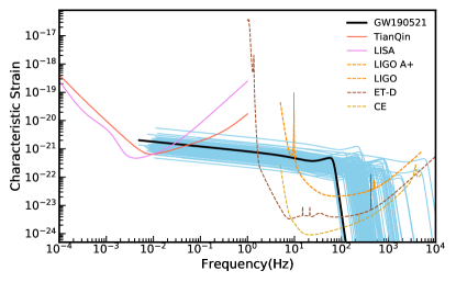
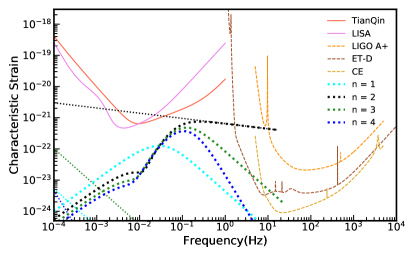
In Fig. 1, we plot the characteristic strains of compact binary coalescence from quasicircular binaries, with parameters derived from transient catalogs published by the LIGO-Virgo-KAGRA collabortion, together with the noise amplitudes listed detectors. It can be observed that although GW190521 merges in the higher bands, 10 years before the merger, the early inspiral GWs have a frequency of as low as Hz and locates above the sensitive band of TianQin. We further notice that due to the higher mass, GW190521, which is indicated with the black thick line, can extend to a lower frequency, making it easier to detect with TianQin.
The strength of a GW signal in a detector can be characterized by the signal-to-noise ratio (SNR). For one Michelson interferometer, the SNR accumulated in observation time is as follows Cutler and Flanagan (1994)
| (1) |
where is the GW waveform in frequency domain , denotes the complex conjugate, is the PSD of the interferometer, and are the initial and final GW frequenciesi, respectively, which can be obtained by Cutler and Flanagan (1994)
| (2) |
where , and are chirp mass, coalescence time, and observation time, respectively. Note that when the observation time is equal to the coalescence time, , we truncate the final frequency at the inner stable circular orbit Cutler and Flanagan (1994), with being the total mass. For the case with a signal observed by multiple interferometers simultaneously, the total SNR is
| (3) |
where is the SNR of a th interferometer and is the total number of interferometers. In order to comprehensively explore the observation potential of future space-borne GW detectors for GW190521-like events, we not only consider TQ and TQ I+II but also a joint observation of TianQin and LISA, i.e., TQ+LISA and TQ I+II+LISA. The response functions and orbital motions for TianQin and LISA are described in detail in Liu et al. (2020); Berti et al. (2005) respectively.
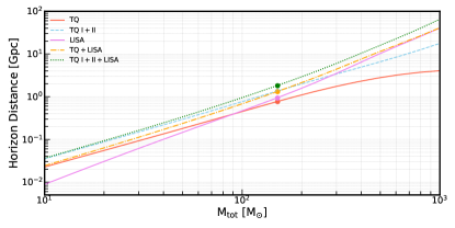
For a binary black hole, the horizion distance of a GW detector, i.e., the maximum detectable distance, could be obtained by solving the Eq. (1) under a given SNR threshold. In Fig. 2, we show the horizon distance of TianQin for the equal mass binary black hole inspirals averaged over sky localization, inclination, and polarization with a total mass between , assuming an SNR threshold for detection. We can see that the horizon distance of TQ grows with the increase of the total masses, because the GWs emitted by heavier sources are stronger, their SNRs are larger. For GW190521-like binaries with a total mass of , TianQin could reach a distance of as far as Gpc.
It is also noted that the horizon distance of TQ increases slowly at the high mass tail, the reason is that for more massive systems, the observation gaps from the “3months on + 3months off” pattern Liu et al. (2020) hinder the SNR accumulation. When TQ I+II is considered, the horizon distance would become about twice that of TQ and show a linear growth, because TQ I+II has no observation gaps. For LISA, the horizon distance is roughly the same as that of TQ I+II, with LISA being more sensitive for binaries with the total mass higher than , but less sensitive when the total mass is smaller than . For TQ+LISA and TQ I+II+LISA, the horizon distance would increase, of which the latter shows more gain. For example, it would be for GW190521, because the latter contains the most detectors. Furthermore, if we consider a further layer of the hierarchical merger model on top of two GW190521-like binaries, i.e., an equal mass binary with the total mass , it could be shown that TianQin (TianQin+LISA) would make detections for sources up to .
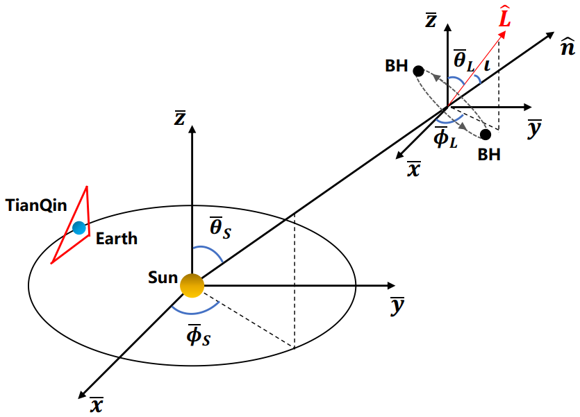
We further examine the detection number of GW190521-like sources in the range within redshift . According to the GW190521-like binary merger rate reported by the LIGO-Virgo collaboration Abbott et al. (2020), we reconstructed the probability density distribution (PDF) by fitting through a log-normal distribution, and 200 random realizations are generated according to this distribution. In each realization, the component masses are set to the median values estimated from GW190521 data. The angular parameters as described in Fig. 3 are distributed uniformly on a sphere. Which means and follow a uniform distribution , while and obey . The overline denotes that we adopt the parameters within the ecliptic coordinate system.
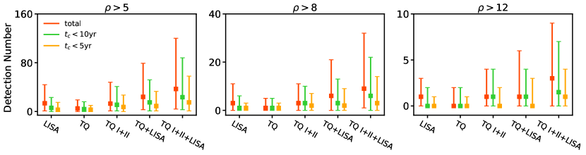
We present the expected detection number over a 5 yr operation time in Fig. 4. With the SNR threshold of TianQin of 12 Liu et al. (2020), TQ or LISA could only make detections in the optimistic scenario. The formation of a network through a number of detectors would improve the detection ability. The expected detection number increases with the order of TQ I+II, TQ+LISA, and TQ I+II+LISA, noticing that a network of TianQin and LISA could detect up to sources. Notice that the coincident observation of multiple detectors could debunk a lot of false alarms, potentially bringing down the SNR threshold Maggiore (2007). Therefore, we also consider the SNR threshold of 8. In the most optimistic scenario, as many as events could be detected. It has been proposed that future ground-based GW detectors can detect SBBH mergers, and trigger a targeted search in space-borne GW detector archive data. Such archival search will be performed in a shrunk parameter space, gaining the potential of further lowering the detection threshold for SNR 5 Wong et al. (2018); Ewing et al. (2021). In such a case, up to sources could be observed with TianQin.
It should be noted that about half of the above sources would merge into ground-based GW detector bands within 10 years, which allows the multiband GW observation. We discuss the parameter estimation precision on these sources later.
II.2 Parameters estimation precision
Assuming the noise to be Gaussian and stationary, for an unbiased estimator of the physical parameters, one can estimate the precision by looking at the covariance matrix, which can be derived with the Fisher information matrix (FIM) method. For one interferometer, the FIM matrix is as follows Cutler and Flanagan (1994)
| (4) |
where is the GW waveform determined by the parameter set . For a network of interferometers, the total FIM is the summation of individual components
| (5) |
where is the FIM of th interferometers. The root mean square of the standard deviation of the th parameter , i.e., the estimation precision, is the square root of the variance, or the component of the covariance matrix , which relates with the FIM through .
We apply the FIM estimate to simulated events with a SNR larger than 8 and will merge within five years, so that an early warning is possible and meaningful. The parameters of sources we consider are . Since the eccentricities of sources at Hz where TianQin is most sensitive are generally lower than 0.1, so we choose at 0.01Hz as a fiducial value Nishizawa et al. (2016). The precision on the sky localization is Berti et al. (2005)
| (6) |
and the error volume of a source is Liu et al. (2020)
| (7) |
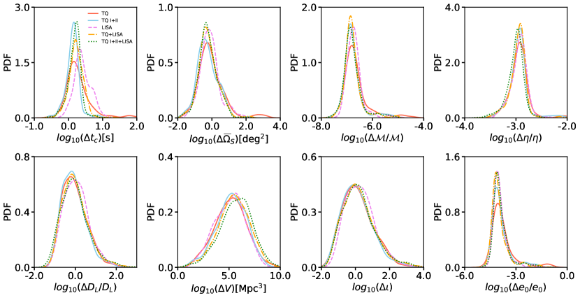
The precision distributions on these parameters are shown in Fig. 5. For TQ, the precision of coalescing time and sky localization is of the order and , respectively. Such high precision in sky localization is achieved through the modulation of the TianQin’s orbital motion Liu et al. (2020). We remark that this precision is vital to the multiband GW observation and multimessenger observation.
In addition, the mass parameters in the waveform phases could also be recovered very accurately, to a relative precision of . This is because the phase evolution is very sensitive to intrinsic parameters like mass, and the precision is inversely proportional to the number of cycles observed, or Cutler and Flanagan (1994). For the other mass parameter, such as the symmetric mass ratio, it also affects the evolution of the waveform phase. However, it is only on higher order terms, so its relative precision is worse, but still could reach .
In comparison, the current ground-based GW observation can only constrain the mass to the accuracy of , which is also prior dependant, with some studies conclude very different mass estimations Abbott et al. (2020); Fishbach and Holz (2020). The space-borne GW detection could easily erase such uncertainty and pinpoint the mass, which would also be important for reconstructing the underlying mass function if multiple events are detected.
For a BBH system, the luminosity distance could be determined to a relative precision of Cutler and Flanagan (1994). With the SNR threshold of , we expect a relative uncertainty of 10% for the luminosity distance. Combining the luminosity distance and sky localization, one could deduce the error volume with Eq. (7). Although the scarcity of the events makes most sources far away and associated with small SNR, both indicators for larger error volumes, one could still expect exceptions of relatively nearby events, with error volumes as small as . On the other hand, the average number density of Milky Way equivalent galaxies is Kyutoku and Seto (2016), which means that one could expect to pinpoint the host galaxy through the GW observation. We discuss the implication of this host galaxy identification on GW cosmology later.
We notice that although the initial orbital eccentricity is set to be a very small number of , TianQin could still observe it with very high precision, with a relative uncertainty of . This precise measurement ability on orbital eccentricity would almost definitely determine the formation channel of such GW190521-like binaries.
Finally, it should be noted that for the networks composed of multiple detectors (TQ I+II, TQ+LISA, and TQ I+II+LISA), the results are similar to those from TQ or LISA. This is because for whatever configurations adopted, the SNR threshold is kept fixed, and the distribution for detected events depends only on the threshold. More detectors are helpful only through the sense that more events can be observed and the loudest event is expected to be associated with higher SNR.
III The capability to constrain the Hubble constant
In this section, we explore the potential of TianQin on constraining cosmology through observation of GW190521-like events. Throughout the work, we assume the underlying cosmology to follow the standard CDM model, where the Hubble parameter can be expressed as
| (8) |
with km/s/Mpc and adopted Ade et al. (2016), where is the redshift, the Hubble constant describes the current expansion rate of the Universe, and and are the fractional densities for total matter and dark energy with respect to the critical density, respectively. The luminosity distance of a BBH in the Universe can be calculated with the Hubble constant and its redshift. As mentioned above, the luminosity distance of a BBH could be determined with GW observation; if the redshift of the galaxy in which the source resides is known, then the Hubble constant could be constrained by fitting the relationship between the luminosity distance and redshift .
We adopt a Bayesian analysis method to infer the Hubble constant from GW190521-like GW detection data and assisting EM observation data Chen et al. (2018); Fishbach et al. (2019); Zhu et al. (2021b). In such case, the likelihood can be written as
| (9) |
where denotes the th event detected, represents the cosmological parameters set, represents all relevant background information, , , and are the polar angle, azimuthal angle, and luminosity, respectively, denotes the galaxy hosting a source, and is the normalization coefficient.
We can factorize the integrand of the numerator in Eq. (9) as
| (10) |
where represents the prior. In this work, we work under the dark standard siren scenario, where we assume no direct observation data of EM counterpart, therefore we can set Chen et al. (2018); Fishbach et al. (2019). We define the prior which is sensitive to the cosmological model, where is the functional relationship between redshift and luminosity distance Hogg (1999). The brighter galaxies generally contain more compact objects, and we assume that the probability of a galaxy hosting a GW190521-like binary is proportional to its -band luminosity, then Fishbach et al. (2019); Gray et al. (2020); Abbott et al. (2021e); Vasylyev and Filippenko (2020). Since the horizon distances of GW190521-like events by both TianQin and LISA are only about Cui et al. (2012); Aghamousa et al. (2016); Gong et al. (2019); Gardner et al. (2006), therefore, we assume the error in the EM survey measurements in our calculations is small and can be safely ignored, , where denotes th event detected (in this work, we adopt a mock galaxy catalog from the MultiDark Planck -body cosmological simulation, obtained from the Theoretical Astrophysical Observatory 222https://tao.asvo.org.au/tao/ Klypin et al. (2016); Croton et al. (2016); Conroy et al. (2010)). Note that the redshift errors caused by the peculiar velocities of galaxies are taken into account in our cosmological analysis, and they are equivalently translated into an additional error of to the GW source in the calculation processes He (2019).
The normalization term can be used to account for selection effects and ensure that the likelihood integrates to unity Chen et al. (2018); Mandel et al. (2019). In this work, we follow the statistical method presented in the literature Zhu et al. (2021b) to evaluate the selection biases of the survey galaxies catalog and calculate the normalization term.
We adopt two methods to count the statistical redshift distribution of candidate host galaxies of GW source, as follows
-
i.
fiducial method: each galaxy in the spatial localization error box of the GW source has equal weight regardless of its position and luminosity information.
-
ii.
weighted method: the weight of a galaxy is related to both its position and -band luminosity.
We adopt the affine-invariant Markov chain Monte Carlo ensemble sampler EMCEE Foreman-Mackey et al. (2013); et al. (2019) to perform the cosmological parameter estimation. Since the detection numbers of GW190521-like events are very uncertain (see Fig. 4), we demonstrate the capability of GW190521-like events to constrain the Hubble constant in the form of the evolution of the constraint precision with the number of GW events, as shown in Fig. 6. In order to eliminate the random fluctuations caused by the specific choice of any event, we repeat this process 48 times independently for each number of GW events, and using the mean value of the constraint errors and credible interval to plot the error bars. Due to the computation limit, we only adopt the GW sources with and use to the analyses of constraining the Hubble constant, because the discarded events can provide little improvements on cosmology constraints.
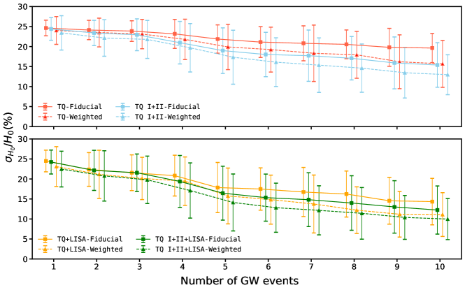
If we assume five GW190521-like events detected, then TQ could constrain the Hubble constant with precisions of about and about , using the fiducial method and weighted method, respectively. Compared with TQ, TQ I+II has a better capability to constrain the Hubble constant. Under the condition of the same number of GW events, the precision of the Hubble constant constrain from TQ I+II using fiducial method slightly outperformed TianQin using the weighted method. With five events, TQ I+II could constrain the Hubble constant with precisions of about and using the fiducial method and the weighted method, respectively.
For the network of multiple space-borne GW detectors, such as TQ+LISA or TQ I+II+LISA, it could significantly improve the capability of the same GW events of constraining the Hubble constant. If we consider the most optimistic scenario where GW190521-like events are detected, for the TQ+LISA configuration, the Hubble constant are expected to be constrained to precisions of about and using the fiducial method and the weighted method, respectively. For the TQ I+II+LISA configuration, the constraint precision of the Hubble constant is expected to achieve the level of about using the weighted method.
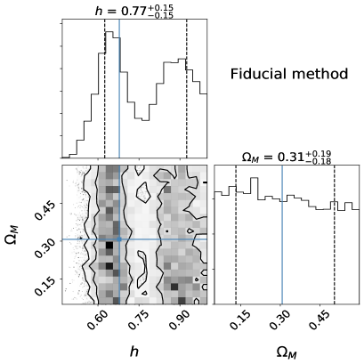
In various detector configurations, compared with the fiducial method, the weighted method could consistently improve the estimation precision of the Hubble constant. To demonstrate the effect of the weighted method on the constraint of the Hubble constant, we show an example of cosmological parameter estimation using the fiducial method and the weighted method, respectively, in Fig. 7. Notice that for the fiducial method, the contamination of galaxies other than the host can cause multiple peaks in the posterior, leading to a worse precision. On the other hand, the weighted method can reliably associate higher weights to the correct host, therefore shrinking the uncertainties.
IV Discussion
In the previous section, we discuss GW190521-like binaries with small orbital eccentricities. However, some theoretical models predict GW190521-like binaries with significant orbital eccentricities could be formed by the dynamical processes Romero-Shaw et al. (2020); Bustillo et al. (2021b); Gayathri et al. (2020). In Fig. 8 we demonstrate how strongly the binary evolution is affected by very large orbital eccentricities.
For the source with small orbital eccentricity, the harmonic is always the dominant mode. The detectability by TianQin or LISA has been demonstrated through the previous section as well as a number of studies Barack and Cutler (2004); Kremer et al. (2018); Randall and Xianyu (2019); D’Orazio and Samsing (2018); Arca-Sedda et al. (2021); Zevin et al. (2019); Chen and Amaro-Seoane (2017); Kremer et al. (2019); Banerjee (2020). However, for the system with very large eccentricity, the harmonic no longer dominates. With the radiation of GWs, the orbital is gradually circularized, harmonic dominates the GW emission at high frequencies. We remark that for such sources, the GW strain they emit at the low frequency range could be too weak for either TianQin or LISA to observe. On the other hand, although the future generation ground-based GW detectors could detect them, with SNR of and for CE and ET-D, respectively Barack and Cutler (2004); Enoki and Nagashima (2007), it would lose the ability to constrain the eccentricity due to the circularization. The expected SNR for space-borne GW detectors is generally small, but one could expect to find the signal through the archival search triggered by ground-based detectors alerts Ewing et al. (2021). Therefore, a null observation in space-borne GW missions could indicate a very high eccentricity, which still contributes significantly to revealing the formation mechanism of GW190521-like binaries.
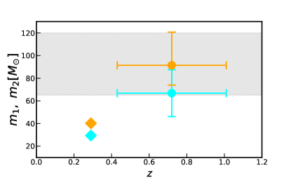
If the LIGO/Virgo estimation of the physical parameters of GW190521 is correct, then future generation ground-based detectors can certainly detect them. However, environment effects could bring a shift to the estimated parameters Chen (2020). For example, if GW190521 orbits around an SMBH, the relative motion between it and the SMBH would cause additional Doppler redshift and gravitational redshift . Such effects could bring a bias in the redshifted mass by a factor of as high as 3 Chen (2020). Under this extreme scenario, the component masses of GW190521 would become as small as and , which could avoid the mass gap issue as shown in Fig. 9. Again, due to the short duration of the signal at high frequencies, ground-based detectors could not effectively resolve degeneracy raised by such environment effects. While the long duration nature of space-borne detections could help track the evolution of redshift and decipher the environment Toubiana et al. (2021).
V Conclusion
In this work, we explore the detection capability of TianQin for GW190521-like binaries with small eccentricities, i.e., horizon distance, detection number, and parameter precision. In addition, we examine the improvement from multiple detectors (TQ I+II, TQ+LISA, and TQ I+II+LISA) compared with single detector. We also discuss the application potential of such sources to GW cosmology.
For GW190521-like binaries, the horizon distance of TianQin is , and the joint observation of TianQin and LISA could reach to . By adopting an SNR threshold of 12, TianQin or LISA could detect a few events, while the joint observation of TianQin and LISA would improve the detection number to about 10. Lowering the threshold to eight doubles the expected detection number. If we consider the scenario of merger-triggered archival search, then it is possible to further lower the threshold to five, where TianQin (TianQin+LISA) could detect dozens (up to a hundred) events. It is worth noting that about half of such sources would merge in several years, making them ideal multiband candidates.
We use FIM to estimate parameter precision, considering multiband sources with SNR greater than 8 and will merge within five years. We conclude that TQ could accurately estimate the parameters, with the coalescence time and sky localization determined to the precision of and , respectively. This implies that TQ could predict when and where these sources would merge. Such potential of early warning could help get facilities prepared to achieve multiband GW observations and multimessenger observations, bringing hope to provide a better test of GR and more detailed study on surrounding environments. We deduce that the error volumes of some loud sources could be smaller than , indicating a direct pinpointing of the host galaxies, which makes them ideal sources to perform GW cosmology study and put constraints on the Hubble constant. The orbital eccentricities could be measured to a relative precision of , which could help us to determine the formation mechanisms: from dynamical interaction in dense stellar clusters or isolated binary evolution. Finally, the relative precision for chirp mass brings hope for the measurement of the mass function of IMBHs merged from GW190521-like binaries. In the typical realization, TQ or TQ I+II could detect about five GW190521-like events, the constraint precision of the Hubble constant are around for TQ and TQ I+II. Both the weighted method and the detector network could significantly improve the capability to constrain the Hubble constant. In the optimistic scenario, if the network detects 10 GW190521-like events, using the weighted method, the constraint on the Hubble constant could reach a precision of .
We also discuss the possibility of detecting very eccentric GW190521-like binaries with TianQin or LISA. Although TianQin or LISA might miss the very eccentric binaries, the null detections could still contribute to the deeper understanding of the sources by putting stringent constraints on orbital eccentricities. TianQin could also help to break possible degeneracy raised by environment effects.
Furthermore, it should be noted that the sources whose SNRs are below a given SNR threshold would form self noise Karnesis et al. (2021), and it is not considered in our calculation. The formed noise would still be below the noise sensitivity Karnesis et al. (2021); Liang et al. (2021), so we believe that our conclusions should be robust. We will study the implication of the self noise on the detectability in future.
Acknowledgements.
This work has been supported by the fellowship of China Postdoctroral Science Foundation (Grant No. 2021TQ0389), the Natural Science Foundation of China (Grants No. 12173104, No. 11805286, No. 91636111, and No. 11690022), Guangdong Major Project of Basic and Applied Basic Research (Grant No. 2019B030302001). The authors acknowledge the uses of the calculating utilities of NUMPY van der Walt et al. (2011), SCIPY Virtanen et al. (2020), and EMCEE Foreman-Mackey et al. (2013); et al. (2019), and the plotting utilities of MATPLOTLIBHunter (2007). The authors also thank Chang Liu, Zheng-Cheng Liang, Xiang-Yu Lyu, Shun-Jia Huang, and Jian-Wei Mei for helpful discussions.References
- Aasi et al. (2015) J. Aasi et al. (LIGO Scientific), Class. Quant. Grav. 32, 074001 (2015), arXiv:1411.4547 [gr-qc] .
- Acernese et al. (2015) F. Acernese et al. (VIRGO), Class. Quant. Grav. 32, 024001 (2015), arXiv:1408.3978 [gr-qc] .
- Abbott et al. (2019a) B. P. Abbott et al. (LIGO Scientific, Virgo), Phys. Rev. X 9, 031040 (2019a), arXiv:1811.12907 [astro-ph.HE] .
- Abbott et al. (2021a) R. Abbott et al. (LIGO Scientific, Virgo), Phys. Rev. X 11, 021053 (2021a), arXiv:2010.14527 [gr-qc] .
- Abbott et al. (2021b) R. Abbott et al. (LIGO Scientific, KAGRA, VIRGO), Astrophys. J. Lett. 915, L5 (2021b), arXiv:2106.15163 [astro-ph.HE] .
- Abbott et al. (2021c) R. Abbott et al. (LIGO Scientific, VIRGO), (2021c), arXiv:2108.01045 [gr-qc] .
- Abbott et al. (2021d) R. Abbott et al. (LIGO Scientific, VIRGO, KAGRA), (2021d), arXiv:2111.03606 [gr-qc] .
- Abbott et al. (2020) R. Abbott et al. (LIGO Scientific, Virgo), Phys. Rev. Lett. 125, 101102 (2020), arXiv:2009.01075 [gr-qc] .
- Heger and Woosley (2002) A. Heger and S. E. Woosley, Astrophys. J. 567, 532 (2002), arXiv:astro-ph/0107037 .
- Belczynski et al. (2016) K. Belczynski et al., Astron. Astrophys. 594, A97 (2016), arXiv:1607.03116 [astro-ph.HE] .
- Woosley (2017) S. E. Woosley, Astrophys. J. 836, 244 (2017), arXiv:1608.08939 [astro-ph.HE] .
- Spera and Mapelli (2017) M. Spera and M. Mapelli, Mon. Not. Roy. Astron. Soc. 470, 4739 (2017), arXiv:1706.06109 [astro-ph.SR] .
- Marchant et al. (2018) P. Marchant, M. Renzo, R. Farmer, K. M. W. Pappas, R. E. Taam, S. de Mink, and V. Kalogera, (2018), 10.3847/1538-4357/ab3426, arXiv:1810.13412 [astro-ph.HE] .
- Vink et al. (2020) J. S. Vink, E. R. Higgins, A. A. C. Sander, and G. N. Sabhahit, (2020), 10.1093/mnras/stab842, arXiv:2010.11730 [astro-ph.HE] .
- Tanikawa et al. (2021) A. Tanikawa, T. Kinugawa, T. Yoshida, K. Hijikawa, and H. Umeda, Mon. Not. Roy. Astron. Soc. 505, 2170 (2021), arXiv:2010.07616 [astro-ph.HE] .
- Costa et al. (2021) G. Costa, A. Bressan, M. Mapelli, P. Marigo, G. Iorio, and M. Spera, Mon. Not. Roy. Astron. Soc. 501, 4514 (2021), arXiv:2010.02242 [astro-ph.SR] .
- Farrell et al. (2021) E. J. Farrell, J. H. Groh, R. Hirschi, L. Murphy, E. Kaiser, S. Ekström, C. Georgy, and G. Meynet, Mon. Not. Roy. Astron. Soc. 502, L40 (2021), arXiv:2009.06585 [astro-ph.SR] .
- Fragione et al. (2020) G. Fragione, A. Loeb, and F. A. Rasio, Astrophys. J. Lett. 902, L26 (2020), arXiv:2009.05065 [astro-ph.GA] .
- Martinez et al. (2020) M. A. S. Martinez et al., Astrophys. J. 903, 67 (2020), arXiv:2009.08468 [astro-ph.GA] .
- Samsing and Hotokezaka (2020) J. Samsing and K. Hotokezaka, (2020), arXiv:2006.09744 [astro-ph.HE] .
- Anagnostou et al. (2020) O. Anagnostou, M. Trenti, and A. Melatos, (2020), arXiv:2010.06161 [astro-ph.HE] .
- Gerosa and Fishbach (2021) D. Gerosa and M. Fishbach, Nature Astron. 5, 8 (2021), arXiv:2105.03439 [astro-ph.HE] .
- Wang et al. (2021) Y.-Z. Wang, S.-P. Tang, Y.-F. Liang, M.-Z. Han, X. Li, Z.-P. Jin, Y.-Z. Fan, and D.-M. Wei, Astrophys. J. 913, 42 (2021), arXiv:2104.02566 [astro-ph.HE] .
- Mapelli et al. (2021) M. Mapelli et al., Mon. Not. Roy. Astron. Soc. 505, 339 (2021), arXiv:2103.05016 [astro-ph.HE] .
- Tagawa et al. (2021) H. Tagawa, B. Kocsis, Z. Haiman, I. Bartos, K. Omukai, and J. Samsing, Astrophys. J. 908, 194 (2021), arXiv:2012.00011 [astro-ph.HE] .
- Kimball et al. (2021) C. Kimball et al., Astrophys. J. Lett. 915, L35 (2021), arXiv:2011.05332 [astro-ph.HE] .
- Liu and Lai (2021) B. Liu and D. Lai, Mon. Not. Roy. Astron. Soc. 502, 2049 (2021), arXiv:2009.10068 [astro-ph.HE] .
- Di Carlo et al. (2019) U. N. Di Carlo, N. Giacobbo, M. Mapelli, M. Pasquato, M. Spera, L. Wang, and F. Haardt, Mon. Not. Roy. Astron. Soc. 487, 2947 (2019), arXiv:1901.00863 [astro-ph.HE] .
- Di Carlo et al. (2020) U. N. Di Carlo, M. Mapelli, Y. Bouffanais, N. Giacobbo, F. Santoliquido, A. Bressan, M. Spera, and F. Haardt, Mon. Not. Roy. Astron. Soc. 497, 1043 (2020), arXiv:1911.01434 [astro-ph.HE] .
- Kremer et al. (2020) K. Kremer, M. Spera, D. Becker, S. Chatterjee, U. N. Di Carlo, G. Fragione, C. L. Rodriguez, C. S. Ye, and F. A. Rasio, Astrophys. J. 903, 45 (2020), arXiv:2006.10771 [astro-ph.HE] .
- Renzo et al. (2020) M. Renzo, M. Cantiello, B. D. Metzger, and Y. F. Jiang, Astrophys. J. Lett. 904, L13 (2020), arXiv:2010.00705 [astro-ph.SR] .
- Safarzadeh and Haiman (2020) M. Safarzadeh and Z. Haiman, Astrophys. J. Lett. 903, L21 (2020), arXiv:2009.09320 [astro-ph.HE] .
- Natarajan (2021) P. Natarajan, Mon. Not. Roy. Astron. Soc. 501, 1413 (2021), arXiv:2009.09156 [astro-ph.GA] .
- Liu and Bromm (2020) B. Liu and V. Bromm, Astrophys. J. Lett. 903, L40 (2020), arXiv:2009.11447 [astro-ph.GA] .
- Cruz-Osorio et al. (2021) A. Cruz-Osorio, F. D. Lora-Clavijo, and C. Herdeiro, JCAP 07, 032 (2021), arXiv:2101.01705 [astro-ph.HE] .
- Rice and Zhang (2021) J. R. Rice and B. Zhang, Astrophys. J. 908, 59 (2021), arXiv:2009.11326 [astro-ph.HE] .
- Samsing et al. (2014) J. Samsing, M. MacLeod, and E. Ramirez-Ruiz, Astrophys. J. 784, 71 (2014), arXiv:1308.2964 [astro-ph.HE] .
- Antonini et al. (2016) F. Antonini, S. Chatterjee, C. L. Rodriguez, M. Morscher, B. Pattabiraman, V. Kalogera, and F. A. Rasio, Astrophys. J. 816, 65 (2016), arXiv:1509.05080 [astro-ph.GA] .
- Nishizawa et al. (2016) A. Nishizawa, E. Berti, A. Klein, and A. Sesana, Phys. Rev. D 94, 064020 (2016), arXiv:1605.01341 [gr-qc] .
- Breivik et al. (2016) K. Breivik, C. L. Rodriguez, S. L. Larson, V. Kalogera, and F. A. Rasio, Astrophys. J. Lett. 830, L18 (2016), arXiv:1606.09558 [astro-ph.GA] .
- Chen and Amaro-Seoane (2017) X. Chen and P. Amaro-Seoane, Astrophys. J. Lett. 842, L2 (2017), arXiv:1702.08479 [astro-ph.HE] .
- Abbott et al. (2019b) B. P. Abbott et al. (LIGO Scientific, Virgo), Astrophys. J. Lett. 882, L24 (2019b), arXiv:1811.12940 [astro-ph.HE] .
- Samsing and D’Orazio (2018) J. Samsing and D. J. D’Orazio, Mon. Not. Roy. Astron. Soc. 481, 5445 (2018), arXiv:1804.06519 [astro-ph.HE] .
- Kremer et al. (2019) K. Kremer et al., Phys. Rev. D 99, 063003 (2019), arXiv:1811.11812 [astro-ph.HE] .
- Carr et al. (2021) B. Carr, S. Clesse, J. García-Bellido, and F. Kühnel, Phys. Dark Univ. 31, 100755 (2021), arXiv:1906.08217 [astro-ph.CO] .
- De Luca et al. (2021) V. De Luca, V. Desjacques, G. Franciolini, P. Pani, and A. Riotto, Phys. Rev. Lett. 126, 051101 (2021), arXiv:2009.01728 [astro-ph.CO] .
- Clesse and Garcia-Bellido (2020) S. Clesse and J. Garcia-Bellido, (2020), arXiv:2007.06481 [astro-ph.CO] .
- Liu and Bromm (2021) B. Liu and V. Bromm, (2021), 10.1093/mnras/stab2028, arXiv:2106.02244 [astro-ph.GA] .
- Sakstein et al. (2020) J. Sakstein, D. Croon, S. D. McDermott, M. C. Straight, and E. J. Baxter, Phys. Rev. Lett. 125, 261105 (2020), arXiv:2009.01213 [gr-qc] .
- Palmese and Conselice (2021) A. Palmese and C. J. Conselice, Phys. Rev. Lett. 126, 181103 (2021), arXiv:2009.10688 [astro-ph.GA] .
- Antoniou (2020) I. Antoniou, (2020), arXiv:2010.05354 [gr-qc] .
- Bustillo et al. (2021a) J. C. Bustillo, N. Sanchis-Gual, A. Torres-Forné, J. A. Font, A. Vajpeyi, R. Smith, C. Herdeiro, E. Radu, and S. H. W. Leong, Phys. Rev. Lett. 126, 081101 (2021a), arXiv:2009.05376 [gr-qc] .
- Fishbach and Holz (2020) M. Fishbach and D. E. Holz, Astrophys. J. Lett. 904, L26 (2020), arXiv:2009.05472 [astro-ph.HE] .
- Miller and Colbert (2004) M. C. Miller and E. J. M. Colbert, Int. J. Mod. Phys. D 13, 1 (2004), arXiv:astro-ph/0308402 .
- van der Marel (2003) R. P. van der Marel, in Carnegie Observatories Centennial Symposium. 1. Coevolution of Black Holes and Galaxies (2003) arXiv:astro-ph/0302101 .
- Volonteri (2010) M. Volonteri, Astron. Astrophys. Rev. 18, 279 (2010), arXiv:1003.4404 [astro-ph.CO] .
- Greene et al. (2020) J. E. Greene, J. Strader, and L. C. Ho, Ann. Rev. Astron. Astrophys. 58, 257 (2020), arXiv:1911.09678 [astro-ph.GA] .
- Fryer et al. (2001) C. L. Fryer, S. E. Woosley, and A. Heger, Astrophys. J. 550, 372 (2001), arXiv:astro-ph/0007176 .
- Heger et al. (2003) A. Heger, C. L. Fryer, S. E. Woosley, N. Langer, and D. H. Hartmann, Astrophys. J. 591, 288 (2003), arXiv:astro-ph/0212469 .
- Loeb and Rasio (1994) A. Loeb and F. A. Rasio, Astrophys. J. 432, 52 (1994), arXiv:astro-ph/9401026 .
- Bromm and Loeb (2003) V. Bromm and A. Loeb, Astrophys. J. 596, 34 (2003), arXiv:astro-ph/0212400 .
- Lodato and Natarajan (2006) G. Lodato and P. Natarajan, Mon. Not. Roy. Astron. Soc. 371, 1813 (2006), arXiv:astro-ph/0606159 .
- Miller and Hamilton (2002) M. C. Miller and D. P. Hamilton, Mon. Not. Roy. Astron. Soc. 330, 232 (2002), arXiv:astro-ph/0106188 .
- O’Leary et al. (2006) R. M. O’Leary, F. A. Rasio, J. M. Fregeau, N. Ivanova, and R. W. O’Shaughnessy, Astrophys. J. 637, 937 (2006), arXiv:astro-ph/0508224 .
- Giersz et al. (2015) M. Giersz, N. Leigh, A. Hypki, N. Lützgendorf, and A. Askar, Monthly Notices of the Royal Astronomical Society 454, 3150 (2015), arXiv:1506.05234 [astro-ph.GA] .
- Portegies Zwart and McMillan (2002) S. F. Portegies Zwart and S. L. W. McMillan, Astrophys. J. 576, 899 (2002), arXiv:astro-ph/0201055 .
- Atakan Gurkan et al. (2004) M. Atakan Gurkan, M. Freitag, and F. A. Rasio, Astrophys. J. 604, 632 (2004), arXiv:astro-ph/0308449 .
- Portegies Zwart et al. (2004) S. F. Portegies Zwart, H. Baumgardt, P. Hut, J. Makino, and S. L. W. McMillan, Nature 428, 724 (2004), arXiv:astro-ph/0402622 .
- Mezcua et al. (2015) M. Mezcua, T. P. Roberts, A. P. Lobanov, and A. D. Sutton, Mon. Not. Roy. Astron. Soc. 448, 1893 (2015), arXiv:1501.04897 [astro-ph.GA] .
- Mezcua (2017) M. Mezcua, Int. J. Mod. Phys. D 26, 1730021 (2017), arXiv:1705.09667 [astro-ph.GA] .
- Wang et al. (2015) S. Wang, J. Liu, Y. Bai, and J. Guo, Astrophys. J. Lett. 812, L34 (2015), arXiv:1510.00233 [astro-ph.SR] .
- Kaaret et al. (2017) P. Kaaret, H. Feng, and T. P. Roberts, Ann. Rev. Astron. Astrophys. 55, 303 (2017), arXiv:1703.10728 [astro-ph.HE] .
- Lin et al. (2020) D. Lin, J. Strader, A. J. Romanowsky, J. A. Irwin, O. Godet, D. Barret, N. A. Webb, J. Homan, and R. A. Remillard, Astrophys. J. Lett. 892, L25 (2020), arXiv:2002.04618 [astro-ph.HE] .
- Baldassare et al. (2016) V. F. Baldassare, A. E. Reines, E. Gallo, J. E. Greene, O. Graur, M. Geha, K. Hainline, C. M. Carroll, and R. C. Hickox, Astrophys. J. 829, 57 (2016), arXiv:1605.05731 [astro-ph.GA] .
- Baldassare et al. (2017) V. F. Baldassare, A. E. Reines, E. Gallo, and J. E. Greene, Astrophys. J. 836, 20 (2017), arXiv:1609.07148 [astro-ph.HE] .
- Mezcua et al. (2018) M. Mezcua, F. Civano, S. Marchesi, H. Suh, G. Fabbiano, and M. Volonteri, Mon. Not. Roy. Astron. Soc. 478, 2576 (2018).
- Amaro-Seoane et al. (2017) P. Amaro-Seoane et al. (LISA), (2017), arXiv:1702.00786 [astro-ph.IM] .
- Toubiana et al. (2021) A. Toubiana et al., Phys. Rev. Lett. 126, 101105 (2021), arXiv:2010.06056 [astro-ph.HE] .
- Mandel et al. (2018) I. Mandel, A. Sesana, and A. Vecchio, Class. Quant. Grav. 35, 054004 (2018), arXiv:1710.11187 [astro-ph.HE] .
- Holgado et al. (2021) A. M. Holgado, A. Ortega, and C. L. Rodriguez, Astrophys. J. Lett. 909, L24 (2021), arXiv:2012.09169 [astro-ph.HE] .
- Mastrogiovanni et al. (2021) S. Mastrogiovanni, L. Haegel, C. Karathanasis, I. M. n. Hernandez, and D. A. Steer, JCAP 02, 043 (2021), arXiv:2010.04047 [gr-qc] .
- Chen et al. (2020) H.-Y. Chen, C.-J. Haster, S. Vitale, W. M. Farr, and M. Isi, (2020), arXiv:2009.14057 [astro-ph.CO] .
- Mukherjee et al. (2020) S. Mukherjee, A. Ghosh, M. J. Graham, C. Karathanasis, M. M. Kasliwal, I. Magaña Hernandez, S. M. Nissanke, A. Silvestri, and B. D. Wandelt, (2020), arXiv:2009.14199 [astro-ph.CO] .
- Gayathri et al. (2021) V. Gayathri, J. Healy, J. Lange, B. O’Brien, M. Szczepanczyk, I. Bartos, M. Campanelli, S. Klimenko, C. O. Lousto, and R. O’Shaughnessy, Astrophys. J. Lett. 908, L34 (2021).
- Luo et al. (2016) J. Luo et al. (TianQin), Class. Quant. Grav. 33, 035010 (2016), arXiv:1512.02076 [astro-ph.IM] .
- Liu et al. (2020) S. Liu, Y.-M. Hu, J.-d. Zhang, and J. Mei, Phys. Rev. D 101, 103027 (2020), arXiv:2004.14242 [astro-ph.HE] .
- Zhu et al. (2021a) L.-G. Zhu, L.-H. Xie, Y.-M. Hu, S. Liu, E.-K. Li, N. R. Napolitano, B.-T. Tang, J.-d. Zhang, and J. Mei, (2021a), arXiv:2110.05224 [astro-ph.CO] .
- Ade et al. (2016) P. A. R. Ade et al. (Planck), Astron. Astrophys. 594, A13 (2016), arXiv:1502.01589 [astro-ph.CO] .
- Peters and Mathews (1963) P. C. Peters and J. Mathews, Phys. Rev. 131, 435 (1963).
- Peters (1964) P. C. Peters, Phys. Rev. 136, B1224 (1964).
- Mangiagli et al. (2019) A. Mangiagli, A. Klein, A. Sesana, E. Barausse, and M. Colpi, Phys. Rev. D 99, 064056 (2019), arXiv:1811.01805 [gr-qc] .
- Krolak et al. (1995) A. Krolak, K. D. Kokkotas, and G. Schaefer, Phys. Rev. D 52, 2089 (1995), arXiv:gr-qc/9503013 .
- Buonanno et al. (2009) A. Buonanno, B. Iyer, E. Ochsner, Y. Pan, and B. S. Sathyaprakash, Phys. Rev. D 80, 084043 (2009), arXiv:0907.0700 [gr-qc] .
- Feng et al. (2019) W.-F. Feng, H.-T. Wang, X.-C. Hu, Y.-M. Hu, and Y. Wang, Phys. Rev. D 99, 123002 (2019), arXiv:1901.02159 [astro-ph.IM] .
- Wang et al. (2019) H.-T. Wang et al., Phys. Rev. D 100, 043003 (2019), arXiv:1902.04423 [astro-ph.HE] .
- Huang et al. (2020) S.-J. Huang, Y.-M. Hu, V. Korol, P.-C. Li, Z.-C. Liang, Y. Lu, H.-T. Wang, S. Yu, and J. Mei, Phys. Rev. D 102, 063021 (2020), arXiv:2005.07889 [astro-ph.HE] .
- Liang et al. (2021) Z.-C. Liang, Y.-M. Hu, Y. Jiang, J. Cheng, J.-d. Zhang, and J. Mei, (2021), arXiv:2107.08643 [astro-ph.CO] .
- Robson et al. (2019) T. Robson, N. J. Cornish, and C. Liu, Class. Quant. Grav. 36, 105011 (2019), arXiv:1803.01944 [astro-ph.HE] .
- Abbott et al. (2017) B. P. Abbott et al. (LIGO Scientific), Class. Quant. Grav. 34, 044001 (2017), arXiv:1607.08697 [astro-ph.IM] .
- Reitze et al. (2019) D. Reitze et al., Bull. Am. Astron. Soc. 51, 035 (2019), arXiv:1907.04833 [astro-ph.IM] .
- Hild et al. (2011) S. Hild et al., Class. Quant. Grav. 28, 094013 (2011), arXiv:1012.0908 [gr-qc] .
- Cutler and Flanagan (1994) C. Cutler and E. E. Flanagan, Phys. Rev. D 49, 2658 (1994), arXiv:gr-qc/9402014 .
- Berti et al. (2005) E. Berti, A. Buonanno, and C. M. Will, Phys. Rev. D 71, 084025 (2005), arXiv:gr-qc/0411129 .
- Maggiore (2007) M. Maggiore, Gravitational Waves. Vol. 1: Theory and Experiments, Oxford Master Series in Physics (Oxford University Press, 2007).
- Wong et al. (2018) K. W. K. Wong, E. D. Kovetz, C. Cutler, and E. Berti, Phys. Rev. Lett. 121, 251102 (2018), arXiv:1808.08247 [astro-ph.HE] .
- Ewing et al. (2021) B. Ewing, S. Sachdev, S. Borhanian, and B. S. Sathyaprakash, Phys. Rev. D 103, 023025 (2021), arXiv:2011.03036 [gr-qc] .
- Kyutoku and Seto (2016) K. Kyutoku and N. Seto, Mon. Not. Roy. Astron. Soc. 462, 2177 (2016), arXiv:1606.02298 [astro-ph.HE] .
- Chen et al. (2018) H.-Y. Chen, M. Fishbach, and D. E. Holz, Nature 562, 545 (2018), arXiv:1712.06531 [astro-ph.CO] .
- Fishbach et al. (2019) M. Fishbach et al. (LIGO Scientific, Virgo), Astrophys. J. Lett. 871, L13 (2019), arXiv:1807.05667 [astro-ph.CO] .
- Zhu et al. (2021b) L.-G. Zhu, Y.-M. Hu, H.-T. Wang, J.-D. Zhang, X.-D. Li, M. Hendry, and J. Mei, (2021b), arXiv:2104.11956 [astro-ph.CO] .
- Hogg (1999) D. W. Hogg, (1999), arXiv:astro-ph/9905116 .
- Gray et al. (2020) R. Gray et al., Phys. Rev. D 101, 122001 (2020), arXiv:1908.06050 [gr-qc] .
- Abbott et al. (2021e) B. P. Abbott et al. (LIGO Scientific, Virgo), Astrophys. J. 909, 218 (2021e), arXiv:1908.06060 [astro-ph.CO] .
- Vasylyev and Filippenko (2020) S. Vasylyev and A. Filippenko, Astrophys. J. 902, 149 (2020), arXiv:2007.11148 [astro-ph.CO] .
- Cui et al. (2012) X.-Q. Cui, Y.-H. Zhao, Y.-Q. Chu, G.-P. Li, Q. Li, L.-P. Zhang, H.-J. Su, Z.-Q. Yao, Y.-N. Wang, X.-Z. Xing, X.-N. Li, Y.-T. Zhu, G. Wang, B.-Z. Gu, A. L. Luo, X.-Q. Xu, Z.-C. Zhang, G.-R. Liu, H.-T. Zhang, D.-H. Yang, S.-Y. Cao, H.-Y. Chen, J.-J. Chen, K.-X. Chen, Y. Chen, J.-R. Chu, L. Feng, X.-F. Gong, Y.-H. Hou, H.-Z. Hu, N.-S. Hu, Z.-W. Hu, L. Jia, F.-H. Jiang, X. Jiang, Z.-B. Jiang, G. Jin, A.-H. Li, Y. Li, Y.-P. Li, G.-Q. Liu, Z.-G. Liu, W.-Z. Lu, Y.-D. Mao, L. Men, Y.-J. Qi, Z.-X. Qi, H.-M. Shi, Z.-H. Tang, Q.-S. Tao, D.-Q. Wang, D. Wang, G.-M. Wang, H. Wang, J.-N. Wang, J. Wang, J.-L. Wang, J.-P. Wang, L. Wang, S.-Q. Wang, Y. Wang, Y.-F. Wang, L.-Z. Xu, Y. Xu, S.-H. Yang, Y. Yu, H. Yuan, X.-Y. Yuan, C. Zhai, J. Zhang, Y.-X. Zhang, Y. Zhang, M. Zhao, F. Zhou, G.-H. Zhou, J. Zhu, and S.-C. Zou, Research in Astronomy and Astrophysics 12, 1197 (2012).
- Aghamousa et al. (2016) A. Aghamousa et al. (DESI), (2016), arXiv:1611.00036 [astro-ph.IM] .
- Gong et al. (2019) Y. Gong, X. Liu, Y. Cao, X. Chen, Z. Fan, R. Li, X.-D. Li, Z. Li, X. Zhang, and H. Zhan, Astrophys. J. 883, 203 (2019), arXiv:1901.04634 [astro-ph.CO] .
- Gardner et al. (2006) J. P. Gardner et al., Space Sci. Rev. 123, 485 (2006), arXiv:astro-ph/0606175 .
- Klypin et al. (2016) A. Klypin, G. Yepes, S. Gottlober, F. Prada, and S. Hess, Mon. Not. Roy. Astron. Soc. 457, 4340 (2016), arXiv:1411.4001 [astro-ph.CO] .
- Croton et al. (2016) D. J. Croton, A. R. H. Stevens, C. Tonini, T. Garel, M. Bernyk, A. Bibiano, L. Hodkinson, S. J. Mutch, G. B. Poole, and G. M. Shattow, Astrophys. J. Suppl. 222, 22 (2016), arXiv:1601.04709 [astro-ph.GA] .
- Conroy et al. (2010) C. Conroy, M. White, and J. E. Gunn, Astrophys. J. 708, 58 (2010), arXiv:0904.0002 [astro-ph.CO] .
- He (2019) J.-h. He, Phys. Rev. D 100, 023527 (2019), arXiv:1903.11254 [astro-ph.CO] .
- Mandel et al. (2019) I. Mandel, W. M. Farr, and J. R. Gair, Mon. Not. Roy. Astron. Soc. 486, 1086 (2019), arXiv:1809.02063 [physics.data-an] .
- Foreman-Mackey et al. (2013) D. Foreman-Mackey, D. W. Hogg, D. Lang, and J. Goodman, Publ. Astron. Soc. Pac. 125, 306 (2013), arXiv:1202.3665 [astro-ph.IM] .
- et al. (2019) F.-M. et al., Journal of Open Source Software 4, 1 (2019), arXiv:1911.07688 [astro-ph.IM] .
- Romero-Shaw et al. (2020) I. M. Romero-Shaw, P. D. Lasky, E. Thrane, and J. C. Bustillo, Astrophys. J. Lett. 903, L5 (2020), arXiv:2009.04771 [astro-ph.HE] .
- Bustillo et al. (2021b) J. C. Bustillo, N. Sanchis-Gual, A. Torres-Forné, and J. A. Font, Phys. Rev. Lett. 126, 201101 (2021b), arXiv:2009.01066 [gr-qc] .
- Gayathri et al. (2020) V. Gayathri, J. Healy, J. Lange, B. O’Brien, M. Szczepanczyk, I. Bartos, M. Campanelli, S. Klimenko, C. Lousto, and R. O’Shaughnessy, (2020), arXiv:2009.05461 [astro-ph.HE] .
- Barack and Cutler (2004) L. Barack and C. Cutler, Phys. Rev. D 69, 082005 (2004), arXiv:gr-qc/0310125 .
- Kremer et al. (2018) K. Kremer, S. Chatterjee, K. Breivik, C. L. Rodriguez, S. L. Larson, and F. A. Rasio, Phys. Rev. Lett. 120, 191103 (2018), arXiv:1802.05661 [astro-ph.HE] .
- Randall and Xianyu (2019) L. Randall and Z.-Z. Xianyu, Astrophys. J. 878, 75 (2019), arXiv:1805.05335 [gr-qc] .
- D’Orazio and Samsing (2018) D. J. D’Orazio and J. Samsing, Mon. Not. Roy. Astron. Soc. 481, 4775 (2018), arXiv:1805.06194 [astro-ph.HE] .
- Arca-Sedda et al. (2021) M. Arca-Sedda, G. Li, and B. Kocsis, Astron. Astrophys. 650, A189 (2021), arXiv:1805.06458 [astro-ph.HE] .
- Zevin et al. (2019) M. Zevin, J. Samsing, C. Rodriguez, C.-J. Haster, and E. Ramirez-Ruiz, Astrophys. J. 871, 91 (2019), arXiv:1810.00901 [astro-ph.HE] .
- Banerjee (2020) S. Banerjee, Phys. Rev. D 102, 103002 (2020), arXiv:2006.14587 [astro-ph.HE] .
- Enoki and Nagashima (2007) M. Enoki and M. Nagashima, Prog. Theor. Phys. 117, 241 (2007), arXiv:astro-ph/0609377 .
- Chen (2020) X. Chen (2020) arXiv:2009.07626 [astro-ph.HE] .
- Karnesis et al. (2021) N. Karnesis, S. Babak, M. Pieroni, N. Cornish, and T. Littenberg, Phys. Rev. D 104, 043019 (2021), arXiv:2103.14598 [astro-ph.IM] .
- van der Walt et al. (2011) S. van der Walt, S. C. Colbert, and G. Varoquaux, Comput. Sci. Eng. 13, 22 (2011), arXiv:1102.1523 [cs.MS] .
- Virtanen et al. (2020) P. Virtanen et al., Nature Meth. 17, 261 (2020), arXiv:1907.10121 [cs.MS] .
- Hunter (2007) J. D. Hunter, Comput. Sci. Eng. 9, 90 (2007).