Evaluating generative networks using Gaussian mixtures of image features

Abstract

We develop a measure for evaluating the performance of generative networks given two sets of images. A popular performance measure currently used to do this is the Fréchet Inception Distance (FID). FID assumes that images featurized using the penultimate layer of Inception-v3 follow a Gaussian distribution, an assumption which cannot be violated if we wish to use FID as a metric. However, we show that Inception-v3 features of the ImageNet dataset are not Gaussian; in particular, every single marginal is not Gaussian. To remedy this problem, we model the featurized images using Gaussian mixture models (GMMs) and compute the $2$-Wasserstein distance restricted to GMMs. We define a performance measure, which we call WaM, on two sets of images by using Inception-v3 (or another classifier) to featurize the images, estimate two GMMs, and use the restricted $2$-Wasserstein distance to compare the GMMs. We experimentally show the advantages of WaM over FID, including how FID is more sensitive than WaM to imperceptible image perturbations. By modelling the non-Gaussian features obtained from Inception-v3 as GMMs and using a GMM metric, we can more accurately evaluate generative network performance.

(a)
$\mu=0$ $\sigma=10$

(b) $\mu_{1},\mu_{2}=-8\sqrt{5},2\sqrt{5}$ $\sigma_{1},\sigma_{2}=2\sqrt{10},\sqrt{15}$ $\pi_{1},\pi_{2}=0.2,0.8$

(c)
$a=-10\sqrt{3}$ $b=10\sqrt{3}$

(d) $\mu_{1},\mu_{2}=-4\sqrt{5},4\sqrt{5}$ $\sigma_{1},\sigma_{2}=2\sqrt{5},2\sqrt{5}$ $\pi_{1},\pi_{2}=0.5,0.5$

(e)
$\mu=0$ $b=5\sqrt{2}$

Figure 1: The FID score between each pair of the distributions shown above is zero although they are clearly different distributions. This is because Equation 1 is only defined for Gaussians, and FID treats any input distribution as Gaussian, even if it is not. We plot one dimensional distributions here for visualization purposes, but the FID score will remain zero even if we extend these distributions to their high dimensional isotrophic counterparts. All that is required for the FID score between two distributions to be zero is that their first two moments match. Figure 1(a) is the only Gaussian distribution. Figures 1(b) and 1(d) are Gaussian mixtures with two components, Figure 1(c) is a uniform distribution, and 1(e) is a Laplace distribution.

1 Introduction

Generative networks, such as generative adversarial networks (GANs) [17] and variational autoencoders [24], model distributions implicitly by trying to learn a map from a simple distribution, such as a Gaussian, to the desired target distribution. Using generative networks, one can generate new images [7, 22, 23, 21, 24], superresolve images [26, 41], solve inverse problems [5], and perform a host of image-to-image translation tasks [20, 43, 42]. However, the high dimensionality of an image distribution makes it difficult to model explicitly, that is, to estimate the moments of the distribution via some parameterization. Just estimating the covariance of a distribution requires $\frac{p(p+1)}{2}$ parameters, where $p$ is the feature dimension. For this reason, modelling distributions implicitly, using transformations of simple distributions, can be useful for high dimensional data. Since the generator network is typically nonlinear, the explicit form of the generated distribution is unknown. Nonetheless, these generative models allow one to sample from the learned distribution.

Because we only have access to samples from these generative networks, instead of explicit probability density functions, evaluating their performance can be difficult. Several ways of evaluating the quality of the samples drawn from generative networks [6] have been proposed, the most popular of which is the Fréchet Inception distance (FID) [19]. FID fits Gaussian distributions to features extracted from a set of a real images and a set of GAN-generated images. The features are typically extracted using the Inception-v3 classifier [37]. These two distributions are then compared using the $2$-Wasserstein [40, 39] metric. While FID has demonstrated its utility in providing a computationally efficient metric for assessing the quality of GAN-generated images, our examination reveals that the fundamental assumption of FID—namely, that the underlying feature distributions are Gaussian—is invalid. A more accurate model of the underlying features will capture a more comprehensive and informative assessment of GAN quality.

In this paper, we first show that the features used to calculate FID are not Gaussian, violating the main assumption in FID (Section 3). As we depict in Figure 1, this can result in an FID value of $0$ even when the data distributions are completely different. This happens because FID only captures the first two moments of the feature distribution and completely ignores all information present in the higher order moments. Thus, FID is biased toward artificially low values and invariant to information present in the higher order moments of the featurized real and generated data.

Thus, we propose a Gaussian mixture model (GMM) [30] for the features instead for several reasons. First, GMMs can model complex distributions and capture higher order moments. In fact, any distribution can be approximated arbitrarily well with a GMM [12]. Second, GMMs are estimated efficiently on both CPU and GPU. Third, there exists a Wasserstein-type metric for GMMs [12] (Section 4) which allows us to generalize FID. We use this newly developed metric from optimal transport to construct our generative model evaluation metric, WaM.

We show that WaM is not as sensitive to visually imperceptible noise as FID (Section 5). This is important because we do not want our evaluations metrics to vary widely between different generated datasets if we cannot visually see any difference between them. Since GMMs can capture more information than Gaussians, WaM more accurately identifies differences between sets of images and avoids the low score bias of FID. We therefore reduce the issue of FID being overly sensitive to various noise perturbations [6] by modelling more information in the feature distributions. We test perturbation sensitivity using additive isotropic Gaussian noise and perturbed images which specifically attempt to increase the feature means using backpropagation [29]. The ability of WaM to model more information in the feature distribution makes it a better evaluation metric than FID for generative networks.

2 Related work

2.1 Wasserstein distance

A popular metric from optimal transport [39, 40] is the $p$-Wasserstein metric. Let $X$ be a Polish metric space with a metric $d$. Given $p\in(0,\infty)$ and two distributions $P$ and $Q$ on $X$ with finite moments of order $p$, the $p$-Wasserstein metric is given by

$$\mathcal{W}_{p}(P,Q)=\left(\inf_{\gamma}\int_{X\times X}d(x,y)^{p}d\gamma(x,y)\right)^{\frac{1}{p}}$$

where the infimum is taken over all joint distributions $\gamma$ of $P$ and $Q$. Different values of $p$ yield different metric properties; in image processing, the $1$-Wasserstein metric on discrete spaces is often used and called the earth mover distance [34]. The $2$-Wasserstein metric [15, 31] is often used when comparing Gaussians since there exists a closed form solution. The formula

$$\mathcal{W}_{2}^{2}(\mathcal{N}({\bm{\mu}}_{1},\bm{\Sigma}_{1}),\mathcal{N}({\bm{\mu}}_{2},\bm{\Sigma}_{2}))=\|{\bm{\mu}}_{1}-{\bm{\mu}}_{2}\|_{2}^{2}$$ (1)

$$\hphantom{---}+\text{Tr}(\bm{\Sigma}_{1})+\text{Tr}(\bm{\Sigma}_{2})-2\text{Tr}\Big{(}\big{(}\bm{\Sigma}_{1}^{\frac{1}{2}}\bm{\Sigma}_{2}\bm{\Sigma}_{1}^{\frac{1}{2}}\big{)}^{\frac{1}{2}}\Big{)}$$

is used to calculate the Fréchet Inception distance.

2.2 FID and variants

The Fréchet Inception distance (FID) [19] is a performance measure typically used to evaluate generative networks. In order to compare two sets of images, $X_{1}$ and $X_{2}$, they are featurized using the penultimate layer of the Inception-v3 network to get sets of features $F_{1}$ and $F_{2}$. For ImageNet data, this reduces the dimension of the data from $3\times 224\times 224=$ $150528$ to $2048$. These features are assumed to be Gaussian, allowing Equation 1 to be used to obtain a distance between them.

There are several ways that FID has been improved. One work has shown that FID is biased [11], especially when it is computed using a small number of samples. They show that FID is unbiased asymptotically and show how to estimate the asymptotic value of FID to obtain an unbiased estimate. Others have used a network different from Inception-v3 to evaluate data that is not from ImageNet; for example, a LeNet-like [25] feature extractor can be used for MNIST. In this work we focus on several different ImageNet feature extractors because of their widespread use. Modelling ImageNet features has been improved due to a conditional version of FID [36] which extends FID to conditional distributions, and a class-aware Fréchet distance [27] which models the classes with GMMs. In this work, we do not consider conditional versions of FID, but our work can be extended to fit such a formulation in a straightforward manner. Moreover, we use GMMs over the feature space rather than one component per class as is done in the class-aware Fréchet distance.

The kernel Inception distance [2] is calculated by mapping the image features to a reproducing kernel Hilbert space and then using an unbiased estimate of maximum mean discrepancy to calculate a distance between sets of images. We compare to KID in Appendix B.

Another related metric is called WInD [13]. WInD uses a combination of the $1$-Wasserstein metric on discrete spaces with the $2$-Wasserstein metric on $\mathbb{R}^{p}$. For this reason, it is not a $p$-Wasserstein metric in $\mathbb{R}^{p}$ or between GMMs. For example, if $P$ and $Q$ are a mixture of Dirac delta functions, then the WInD distance between them becomes the $1$-Wasserstein distance. However, if $P$ and $Q$ are Gaussian, then the WInD distance between them becomes the $2$-Wasserstein distance. Moreover, if $P$ and $Q$ are arbitrary GMMs, the relationship between WInD and the $p$-Wasserstein metrics is not clear. This means that WInD can alternate between the $1$-Wasserstein and $2$-Wasserstein distance depending on the input distributions. In this paper, we focus on using a metric which closely follows the $2$-Wasserstein distance as is currently done with FID.

2.3 2-Wasserstein metric on GMMs: $\text{MW}_{2}$

A closed form solution for the $2$-Wasserstein distance between GMMs is not known. This is because the joint distribution between two GMMs is not necessarily a GMM. However, if we restrict ourselves to the relaxed problem of only considering joint distributions over GMMs, then the resulting $2$-Wasserstein distance of this new space is known. The restricted space of GMMs is quite large, since GMMs can approximate any distribution to arbitrary precision given enough mixture components. So given two GMMs, $P$ and $Q$, we can calculate

$$\text{MW}_{2}^{2}(P,Q)=\inf_{\gamma}\int_{X\times X}d(x,y)^{2}d\gamma(x,y)$$

where the infimum is over all joint distributions $\gamma$ which are also GMMs. Constraining the class of joint distributions is a relaxation that has been done before [3] due to the difficulty of considering arbitrary joint distributions. This metric, $\text{MW}_{2}$, appears in a few different sources in the literature [9, 8, 10] and has been studied theoretically [12]; recently, implementations of this quantity have emerged.

The practical formulation of this problem is done as follows. Let $P=\sum_{i=1}^{K_{0}}\pi_{i}\nu_{i}$ and $Q=\sum_{j=1}^{K_{1}}\alpha_{j}\mu_{j}$ be two GMMs with Gaussians $\nu_{i},\mu_{j}$ for $i\in\{1,\dots,K_{0}\},j\in\{1,\dots,K_{1}\}$. Then, we have that

$$\text{MW}_{2}^{2}(P,Q)=\min_{\gamma}\sum_{ij}\gamma_{ij}\mathcal{W}_{2}^{2}(\nu_{i},\mu_{j})$$ (2)

where $\gamma$ is taken to be the joint distribution over the two categorical distributions $\begin{bmatrix}\pi_{1}&\ldots&\pi_{K_{0}}\end{bmatrix}$ and $\begin{bmatrix}\alpha_{1}&\ldots&\alpha_{K_{1}}\end{bmatrix}$; hence, $\gamma$ in this case is actually a matrix. Thus, $\text{MW}_{2}$ can be implemented as a discrete optimal transport plan and efficient software exists to compute this [16].

$\text{MW}_{2}$ is a great candidate for modelling the distance between GMMs for several reasons; most importantly, it is an actual distance metric. Since we are restricting the joint distribution to be a GMM, we see that $\text{MW}_{2}$ must be greater than or equal to the $2$-Wasserstein distance between two GMMs. Moreover, $\text{MW}_{2}$ clearly approximates the $2$-Wasserstein metric; there are bounds showing how close $\text{MW}_{2}$ is to $\mathcal{W}_{2}$ [12]. It is also computationally efficient to compute because it can be formulated as a discrete optimal transport problem, making it practical. The strong theoretical properties and computational efficiency of $\text{MW}_{2}$ make it a prime candidate to calculate the distance between GMMs.

3 Inception-v3 has Non-Gaussian features on ImageNet

3.1 Non-Gaussian features can differ and have zero FID

The calculation of FID assumes that features from the penultimate layer of Inception-v3 [37] are Gaussian. This layer average pools the outputs of several convolutional layers which are rectified via the ReLU activation. Though an argument can be made for why the preactivations of the convolutional layers are Gaussian (using the central limit theorem), the rectified and averaged outputs are not. In fact, they are likely to be averages of rectified Gaussians [1]. Although these features are high dimensional and cannot be visualized, we plot the histograms of a randomly selected feature extracted with Inception-v3, ResNet-18, ResNet-50, and ResNeXt-101 (32$\times$8d) in Figure 2. We construct these histograms using the $50000$ images in the ImageNet validation dataset. We see that none these randomly selected features appear Gaussian.

Figure 2: Histograms showing non-Gaussianity of randomly chosen features from the ImageNet validation dataset featurized by ResNet-18, ResNet-50, ResNeXt-101 (32$\times$8d), and Inception-v3. They are non-negative because these features are passed through a ReLU layer and then average pooled; for this reason, we have a spike around $0$. These histograms are empirical distributions.

If the Gaussian assumption of FID is false, one can achieve low FID values while having drastically different distributions, as shown on Figure 1. This is true in part because FID only considers the first two moments of the distributions being compared; differences in skew and higher order moments are not taken into account in the FID calculation. This can cause FID to be extremely low when the distributions being compared are quite different.

3.2 ImageNet features are not Gaussian

Testing if Inception-v3 features are Gaussian is not trivial because they are 2048-dimensional. Even if each marginal distribution appears Gaussian, we cannot be sure that the joint distribution is Gaussian. However, if the marginals are not Gaussian, this implies that original distribution is not Gaussian. Therefore, we conducted a series of Kolmogorov–Smirnov hypothesis tests [14], a statistical nonparametric goodness-of-fit test that verifies whether an underlying probability distribution, in our case the marginals, differs from a hypothesized distribution, a Gaussian distribution.

We calculated features from the entire ImageNet validation dataset using ResNet-18, ResNet-50, ResNeXt-101 (32$\times$8d), and Inception-v3. For each set of features, we then tested each marginal using the Kolmogorov–Smirnov tests with the hypothesis that the features come from a normal distribution. Using a $p$-value of $0.01$, the test found that $100\%$ of the marginals fail to pass the hypothesis. This confirms, with high certainty, that neither the marginals nor the whole feature distribution is Gaussian.

Since the features of Inception-v3 are not Gaussian, we have a few options. The first option is to use features before the average pooling layer and ReLU operation because these features may actually be Gaussian. However, these features are extremely high dimensional ($64\times 2048=$ $131072$) and thus very hard to estimate accurately. Alternatively, we can remove the ReLU operation, but this would distort the features by removing the nonlinearity that is so critical to deep networks. Another option we have is to use a different network for feature extraction; however, most networks which perform very well on ImageNet have high dimensionality convolutional features followed by ReLU and average pooling, e.g., ResNet-18, ResNet-50, and ResNeXt-101 (32$\times$8d). Moreover, trying to obtain Gaussian features is not a general solution because even if the training data has Gaussian features, new data may not. Therefore, we decided to model these non-Gaussian features using Gaussian mixture models which can capture information past the first two moments of a distribution.

4 WaM — Model details

4.1 A Gaussian mixture model can learn more complex distributions

In this work we use the Gaussian mixture model (GMM) to model non-Gaussian features. GMMs are a generalization of Gaussian distributions (i.e., when the number of components equal $1$) and hence we can generalize FID using the formulas discussed in Section 2.3. Moreover, any distribution can be approximated to arbitrary precision using a GMM [12]. Estimation of GMM parameters are also computationally efficient and have been studied thoroughly [4, 30]. Most importantly, we can calculate the distance between GMMs using equation 2.

Figure 3: AIC curves for features used for picking the number of mixture components $K$. We choose $K=10$ for ResNet-18, $K=40$ for both ResNet-50 and ResNeXt-101 (32$\times$8d), and $K=15$ and Inception-v3.

Before modelling the image features with GMMs, we transform them using a simple element-wise natural logarithm transformation; i.e., ${\bm{x}}^{\prime}=\text{ln}({\bm{x}})$ for features ${\bm{x}}$. This squashes the peak and make the data easier to model [30] although it is still not easily modeled by just one Gaussian distribution.

We calculate our performance metric for generative models by using the $\text{MW}_{2}$ [12] metric for GMMs on GMMs estimated from extracted features of images. The procedure is summarized as follows. We first pick a network, such as Inception-v3, to calculate the features. These features are then used to estimate a GMM with $K$ components. We do this for real data and for generated data. We then calculate the FID of each combination of components, one from the real data GMM and one from the generated data GMM. Then, we solve a discrete optimal transport problem using the $2$-Wasserstein distance squared as the ground distances to obtain WaM. We use $n=$ $50000$ samples because this was shown to be an approximately unbiased [11] estimate of FID. We call our metric WaM since it is a Wasserstein-type metric on GMMs of image features.

We fit the GMM to the data using the expectation maximization algorithm implemented in scikit-learn [33] and pycave. We model the features with full covariance matrices so that we are truly generalizing FID. One can fit diagonal or spherical covariance matrices if speed is required, but this will yield simpler GMMs. We considered several GPU implementations of GMM fitting instead of the scikit-learn CPU implementation. However, the sequential nature of the expectation maximization algorithm caused the run times to be similar for GPU and CPU algorithms.

4.2 Using different networks

In addition to using Inception-v3 for feature extraction, we also use ResNet-18, ResNet-50, and ResNeXt-101 (32$\times$8d) trained on ImageNet. For each network, we use the penultimate layer for feature extraction, as was done originally for Inception-v3. We use ResNet-18 because its features are only $512$-dimensional and hence can be calculated faster than Inception-v3. ResNet-50 performs better than ResNet-18 and so we included it in some of our experiments. Finally, ResNeXt-101 (32$\times$8d) achieves the highest accuracy in the ImageNet classification task of all the pretrained classifiers on Pytorch [32].

4.3 Picking $K$ and fitting the GMM

When modelling features, we must pick the number of components we choose to have in our GMM. If we pick $K=1$ (and use Inception-v3 as our feature extractor), then we just calculate FID. The more components we pick, the better our fit will be. However, if we pick $K$ to be too large, such as $K\geq N$, then we may overfit in the sense that we can have each component centered around single data points. This is clearly not desirable, so we fit all of our GMMs with a maximum of $K=50$ components.

We use the Akaike information criterion (AIC) to choose $K$ since likelihood criteria are well suited for density estimation [30] as compared with cross validation for clustering. However, calculating AIC for multiple components will take significant computation time and power if done every time one wants to calculate WaM. For this reason, we pick a specific $K$ based on the ImageNet validation set. A value for $K$ which models the ImageNet validation dataset well should be a good $K$ for modelling similar image datasets. As shown in Figure 3, the AIC curves have varying shapes. We use the kneed method [35] for our choice of $K$ (using $S=0.5$ in the official implementation ) for the ResNet-18, ResNet-50, ResNeXt-101 (32$\times$8d), and Inception-v3 features. In the calculation of the knee, we ignore the first few points of the plots because desirable knees lie in the convex part of the plot, not the concave part.

Since GMMs have more parameters, they are computationally more expensive to train than simply modelling the data as a Gaussian. However, we use GMM training procedures that take advantage of GPU parallelization. As shown on Table 1, fitting a $20$ component GMM only takes approximately 100 seconds and calculating WaM takes an additional 60 seconds. In these calculations, we compare to a fixed reference dataset with precalculated parameters as is typically done. From empirical observations, FID takes about $20$ seconds to compute, making WaM only $140$ seconds, or about $2$ minutes, slower.

k	5	10	15	20	25	30
GMM Fitting	$51.1$	$83.3$	$78.3$	$99.8$	$143.2$	$139.2$
WaM Calc	$17.4$	$32.2$	$47.1$	$60.3$	$74.6$	$86.9$

Table 1: Average number of seconds it takes to fit a GMM and calculate WaM on one GPU. This makes WaM approximately 2 minutes slower than FID.

5 Experiments

In these experiments we find that WaM performs better than both FID and KID. The KID experiments are in Appendix B.

Original (BigGAN)	Perturbed (BigGAN)	Original (ImageNet)	Perturbed (ImageNet)
$\!\begin{aligned} \text{FID}&=55.71\\ \text{WaM}^{2}&=378.37\end{aligned}$	$\!\begin{aligned} \text{FID}&=154.19\\ \text{WaM}^{2}&=424.29\end{aligned}$	$\!\begin{aligned} \text{FID}&=3.66\\ \text{WaM}^{2}&=237.05\end{aligned}$	$\!\begin{aligned} \text{FID}&=46.63\\ \text{WaM}^{2}&=280.02\end{aligned}$
$\!\begin{aligned} R_{\text{FID}}&=2.77\\ R_{\text{WaM}}&=1.12\\ R&=2.47\end{aligned}$		$\!\begin{aligned} R_{\text{FID}}&=12.74\\ R_{\text{WaM}}&=1.18\\ R&=10.78\end{aligned}$

Figure 4: Samples of images showing targeted perturbations which target the feature means, as defined on Equation 3. The two original images above are randomly selected from a set of $50000$ images generated by BigGAN and a set of $50000$ images of the ImageNet validation dataset. We cannot visually perceive the difference between the original and perturbed images, despite the datasets from which they were selected clearly demonstrating a drastic change in FID. The FID, WaM, and $R$ values were calculated using Inception-v3.

5.1 Targeted perturbations — WaM captures more information than FID

The purpose of this experiment is to show that WaM can capture more information than FID by implicitly capturing higher order moments. Although features extracted from classifiers are not Gaussian, we do not have a perfect model for them. In fact, it is difficult to come up with distributions of features without images to start with. Thus, we start with a set of images, perturb them in order to change their first and second moments, then calculate WaM and FID on the perturbed images. Since WaM is a generalization of FID, the perturbed images will likely affect both WaM and FID. However, since WaM can capture more information than FID on the feature distributions, we hypothesize that WaM will not be as affected as FID.

We construct these perturbed sets of images by trying to maximize the following losses

$$\mathcal{L}({\bm{\mu}}) =\|{\bm{\mu}}-{\bm{\mu}}_{0}\|_{2}^{2}$$ (3)

$$\mathcal{L}(\bm{\Sigma}) =\|\bm{\Sigma}-\bm{\Sigma}_{0}\|_{F}$$ (4)

$$\mathcal{L}({\bm{\mu}},\bm{\Sigma}) =\frac{1}{2}\Big{(}\|{\bm{\mu}}-{\bm{\mu}}_{0}\|_{2}^{2}+\|\bm{\Sigma}-\bm{\Sigma}_{0}\|_{F}\Big{)}$$ (5)

$$\mathcal{L}(\bm{\Sigma}) =\text{Tr}(\bm{\Sigma})+\text{Tr}(\bm{\Sigma}_{0})-2\text{Tr}\Big{(}\big{(}\bm{\Sigma}^{\frac{1}{2}}\bm{\Sigma}_{0}\bm{\Sigma}^{\frac{1}{2}}\big{)}^{\frac{1}{2}}\Big{)}$$ (6)

using the Fast Gradient Sign Method (FGSM) [18], where ${\bm{\mu}}_{0}$ and $\bm{\Sigma}_{0}$ are the fixed first and second moment of the ImageNet training data. In addition we adversarially perturb FID and report our findings in more detail in Appendix A. In Figure 4 we show how the mean perturbation using Equation 3 affects FID significantly more than WaM even though there are no visual differences.

original	$\sigma=0.01$	$\sigma=0.05$	$\sigma=0.1$	$\sigma=0.2$	$\sigma=0.5$
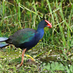
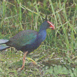
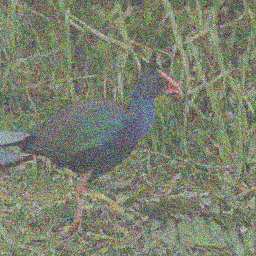
	$\sigma=0.01$	$\sigma=0.05$	$\sigma=0.1$	$\sigma=0.2$	$\sigma=0.5$
FID(orig)	24.14	24.14	24.14	24.14	24.14
FID(pert)	24.37	27.10	33.55	51.10	114.94
WaM2(orig)	504.30	504.30	504.30	504.30	504.30
WaM2(pert)	539.54	516.75	628.68	748.65	$1328.01$
$R_{\text{FID}}$	1.01	1.12	1.39	2.12	4.76
$R_{\text{WaM}}$	1.07	1.02	1.25	1.48	2.63
$R$	0.94	1.10	1.11	1.43	1.81

Figure 5: $R$ values for BigGAN-generated images using additive isotropic Gaussian noise showing that FID is slightly more sensitive than WaM to noise perturbations of generated images. The noise perturbations in this experiment are all greater in magnitude than the targeted perturbations in Section 5.1. The original image above was randomly selected from a set of $50000$ images generated by BigGAN. The FID, WaM, and $R$ values were calculated using ResNet-18.

original	$\sigma=0.01$	$\sigma=0.05$	$\sigma=0.1$	$\sigma=0.2$	$\sigma=0.5$
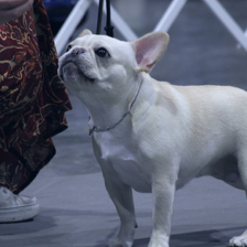
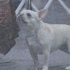
	$\sigma=0.01$	$\sigma=0.05$	$\sigma=0.1$	$\sigma=0.2$	$\sigma=0.5$
FID(orig)	3.61	3.61	3.61	3.61	3.61
FID(pert)	5.07	21.79	52.30	120.05	322.84
WaM2(orig)	208.45	208.45	208.45	208.45	208.45
WaM2(pert)	219.49	316.06	549.03	1081.28	4007.29
$R_{\text{FID}}$	1.41	6.04	14.49	33.26	89.45
$R_{\text{WaM}}$	1.05	1.52	2.63	5.19	19.22
$R$	1.34	3.98	5.50	6.41	4.65

Figure 6: $R$ values for real images (ImageNet validation data) using additive isotropic Gaussian noise showing that FID is significantly more sensitive than WaM to noise perturbations of real images. The noise perturbations in this experiment are all greater in magnitude than the targeted perturbations in Section 5.1. The original image above was randomly selected from a set of $50000$ images of the ImageNet validation dataset. In contrast to Figure 5, we see that FID is more sensitive to these perturbations when the images look more realistic. The FID and WaM values were calculated using ResNet-18.

To calculate FID or WaM, we must compare two sets of images; thus, we always compare to the ImageNet training set [7]. This allows us to calculate the FID and WaM of the ImageNet training set against real images from the ImageNet validation set, generated images from BigGAN [7], and perturbed images from each. We compare to real images because we want our metrics to work well with the most realistic images possible, given the continuously improving nature of GANs. We used $50000$ images for doing all the comparisons and the whole training set for the reference. To produce the adversarial images, we extracted the features from all the $50000$ ImageNet validation images, then ran FGSM with an $\epsilon=0.01$ and batch size of $64$ until we perturbed all $50000$ of our target images (e.g., ImageNet validation set). This means that the maximum difference per pixel is $0.25\%$. During training we calculated the gradients that maximize the losses above between the features of a batch of $64$ images and the features of the ImageNet training set.

Comparing FID and WaM is difficult because they are different metrics with different scales. For this reason, we must normalize them when comparing. Thus, we define $R_{\text{FID}}$ to be the ratio of the FID of the perturbed images over the FID of the original images. Hence, $R_{\text{FID}}$ shows how much FID has increased due to the perturbation. Similarly, we define $R_{\text{WaM}}$ to be the ratio of WaM squared of the perturbed images over WaM squared of the original images. FID is typically reported as the $2$-Wasserstein squared distance, so we square WaM so that it is also a squared distance. Then we define $R=\frac{R_{\text{FID}}}{R_{\text{WaM}}}$ to be the ratio for these two increases. Thus, for $R>1$ we have that FID increased faster than WaM due to perturbation.

When we perturb images generated from BigGAN [7] or the ImageNet training data we cannot visually perceive a difference, as shown in Figure 4. However, for the BigGAN images, FID increases by a factor of $R_{\text{FID}}=2.77$ while WaM only increases by a factor of $R_{\text{WaM}}=1.12$. This difference is even significantly more evident with real images drawn from the ImageNet training data set. We see that the FID score after perturbation increases by $R_{\text{FID}}=12.74$ times. Since WaM only increases by $R_{\text{WaM}}=1.18$ times, we see that FID increased $R=10.78$ times more than WaM for an imperceptible, but targeted, perturbation. That is an extremely large sensitivity to noise that human eyes cannot even see. A metric which reflects perceptual quality perfectly would not be affected whatsoever by these perturbations. Neither FID nor WaM are perfect, but WaM’s lower sensitivity to visually imperceptible perturbation is better aligned with the objective of assessing perceptual quality in images.

Even though these perturbations are targeted to specifically change the first two moments of the data, we note that WaM is still affected by these perturbations. This is because WaM can capture more moments of the data than FID. More specifically, WaM can learn a Gaussian distribution (e.g., if all the components are the same), yet FID and WaM yield different results in this experiment, implying that the features are not modeled well by FID and benefit from the additional information captured by WaM.

5.2 Random perturbations

In this section we show that WaM is also less sensitive than FID to additive isotropic Gaussian noise. We do this by corrupting images generated from BigGAN and the ImageNet training dataset by adding isotropic Gaussian noise with standard deviation $\sigma\in\{0.01,0.05,0.1,0.2,0.5\}$ and then calculating their features. Samples of how these noisy images compare to the original are shown in Figures 5 and 6. In these experiments, we use ResNet-18 to extract the features. The $\epsilon=0.01$ used in Section 5.1 corresponds to approximately $\sigma=0.0014$, meaning that the additive random noise in Figures 5 and 6 perturbs the images much more than the targeted noise in Figure 4.

We see that FID and WaM perform similarly when calculated using noisy BigGAN generated images, but WaM is still significantly more robust than FID (see Figure 5). Moreover, FID skyrockets when calculated using ImageNet training data. This is likely due to FID not being able to capture the differences between the ImageNet training and validation set. One can justly assume that both data sets are sampled from the same distribution; however, we are not comparing the distributions from which they are sampled. We are comparing the two sets of images from the training and validation set, which are not the same. Therefore, FID’s inability to model the correct distribution of features causes it to become extremely sensitive to this noise, even when it is barely visually perceptible. This sensitivity of FID to noise has been noted before [19, 6]. FID is affected $R=5.50$ times as much as WaM when the noise is barely visible ($\sigma=0.1$), making WaM much more desirable to use in noisy contexts (see Figure 6).

A good metric for evaluating generative network performance should be able to capture the quality of generated images at all stages. FID does not do this well. FID is sensitive to noise perturbations, especially when the images look realistic; hence, $R$ is much larger for the ImageNet training data than it is for the BigGAN generated images. As generative networks get better and better, we must use more information (not just the first and second moment) from the feature distribution in order to accurately evaluate generated samples.

6 Conclusions

We generalize the notion of FID by modeling image features with GMMs and computing a relaxed $2$-Wasserstein distance on the distributions. Our proposed metric, WaM, allows us to accurately model more complex distributions than FID, which relies on the invalid assumption that image features follow a Gaussian distribution. Moreover, we show that WaM is less sensitive to both imperceptible targeted perturbations that modify the first two moments of the feature distribution and imperceptible additive Gaussian noise. This is important because we want a performance metric which is truly reflective of the perceptual quality of images and will not vary much when visually imperceptible noise is added. We can use WaM to evaluate networks which generate new images, superresolve images, solve inverse problems, perform image-to-image translation tasks, and more. As networks continue to evolve and generate more realistic images, WaM can provide a superior model of the feature distributions, thus enabling more accurate evaluation of extremely-realistic generated images.

Appendix A Targeted perturbations (extended)

Here we show the targeted perturbation results in more detail than in Section 5.1. We don’t show figures of the images before and after perturbation besides Figure 4 because they are all imperceptible, with maximum pixel differences of $0.25\%$. All the FID, WaM, and $R$ values were calculated using Inception-v3. We use Equation 3 for Table 2, Equation 4 for Table 3, Equation 5 for Table 4, Equation 6 for Table 5, and FID for Table 6. We follow recent work [29, 28] in order to backpropagate through FID. Our results show that in every case, FID is significantly more sensitive to imperceptible perturbations of the first two moments when compared to WaM.

Original (BigGAN)	Perturbed (BigGAN)	Original (ImageNet)	Perturbed (ImageNet)
$\!\begin{aligned} \text{FID}&=55.7\\ \text{WaM}^{2}&=378.4\end{aligned}$	$\!\begin{aligned} \text{FID}&=154.2\\ \text{WaM}^{2}&=424.3\end{aligned}$	$\!\begin{aligned} \text{FID}&=3.7\\ \text{WaM}^{2}&=237.0\end{aligned}$	$\!\begin{aligned} \text{FID}&=46.6\\ \text{WaM}^{2}&=280.0\end{aligned}$
$\!\begin{aligned} R_{\text{FID}}&=2.8\\ R_{\text{WaM}}&=1.1\\ R&=\mathbf{2.5}\end{aligned}$		$\!\begin{aligned} R_{\text{FID}}&=12.7\\ R_{\text{WaM}}&=1.2\\ R&=\mathbf{10.8}\end{aligned}$

Table 2: Mean perturbations: We show that FID values are significantly more sensitive to imperceptible perturbations to the feature means (Equation 3).

Original (BigGAN)	Perturbed (BigGAN)	Original (ImageNet)	Perturbed (ImageNet)
$\!\begin{aligned} \text{FID}&=55.7\\ \text{WaM}^{2}&=378.4\end{aligned}$	$\!\begin{aligned} \text{FID}&=125.7\\ \text{WaM}^{2}&=540.8\end{aligned}$	$\!\begin{aligned} \text{FID}&=3.7\\ \text{WaM}^{2}&=237.0\end{aligned}$	$\!\begin{aligned} \text{FID}&=113.0\\ \text{WaM}^{2}&=422.5\end{aligned}$
$\!\begin{aligned} R_{\text{FID}}&=2.3\\ R_{\text{WaM}}&=1.4\\ R&=\mathbf{1.6}\end{aligned}$		$\!\begin{aligned} R_{\text{FID}}&=30.9\\ R_{\text{WaM}}&=1.8\\ R&=\mathbf{17.3}\end{aligned}$

Table 3: Covariance perturbations: We show that FID values are significantly more sensitive to imperceptible perturbations to the feature covariances (Equation 4).

Original (BigGAN)	Perturbed (BigGAN)	Original (ImageNet)	Perturbed (ImageNet)
$\!\begin{aligned} \text{FID}&=55.7\\ \text{WaM}^{2}&=378.4\end{aligned}$	$\!\begin{aligned} \text{FID}&=177.6\\ \text{WaM}^{2}&=521.3\end{aligned}$	$\!\begin{aligned} \text{FID}&=3.7\\ \text{WaM}^{2}&=237.0\end{aligned}$	$\!\begin{aligned} \text{FID}&=106.9\\ \text{WaM}^{2}&=412.2\end{aligned}$
$\!\begin{aligned} R_{\text{FID}}&=3.2\\ R_{\text{WaM}}&=1.4\\ R&=\mathbf{2.3}\end{aligned}$		$\!\begin{aligned} R_{\text{FID}}&=29.2\\ R_{\text{WaM}}&=1.7\\ R&=\mathbf{16.8}\end{aligned}$

Table 4: Mean-covariance perturbations: We show that FID values are significantly more sensitive to imperceptible perturbations to the feature means and covariances together (Equation 5).

Original (BigGAN)	Perturbed (BigGAN)	Original (ImageNet)	Perturbed (ImageNet)
$\!\begin{aligned} \text{FID}&=55.7\\ \text{WaM}^{2}&=378.4\end{aligned}$	$\!\begin{aligned} \text{FID}&=145.9\\ \text{WaM}^{2}&=578.3\end{aligned}$	$\!\begin{aligned} \text{FID}&=3.7\\ \text{WaM}^{2}&=237.0\end{aligned}$	$\!\begin{aligned} \text{FID}&=112.2\\ \text{WaM}^{2}&=444.0\end{aligned}$
$\!\begin{aligned} R_{\text{FID}}&=2.6\\ R_{\text{WaM}}&=1.5\\ R&=\mathbf{1.7}\end{aligned}$		$\!\begin{aligned} R_{\text{FID}}&=30.7\\ R_{\text{WaM}}&=1.9\\ R&=\mathbf{16.4}\end{aligned}$

Table 5: Alternative covariance perturbations: We show that FID values are significantly more sensitive to imperceptible perturbations to the feature covariances, using a different metric on the covariances than the Frobenius norm (Equation 6).

Original (BigGAN)	Perturbed (BigGAN)	Original (ImageNet)	Perturbed (ImageNet)
$\!\begin{aligned} \text{FID}&=55.7\\ \text{WaM}^{2}&=378.4\end{aligned}$	$\!\begin{aligned} \text{FID}&=166.5\\ \text{WaM}^{2}&=548.5\end{aligned}$	$\!\begin{aligned} \text{FID}&=3.7\\ \text{WaM}^{2}&=237.0\end{aligned}$	$\!\begin{aligned} \text{FID}&=112.0\\ \text{WaM}^{2}&=377.0\end{aligned}$
$\!\begin{aligned} R_{\text{FID}}&=3.0\\ R_{\text{WaM}}&=1.4\\ R&=\mathbf{2.1}\end{aligned}$		$\!\begin{aligned} R_{\text{FID}}&=30.6\\ R_{\text{WaM}}&=1.6\\ R&=\mathbf{19.2}\end{aligned}$

Table 6: FID perturbations: We show that FID values are significantly more sensitive to imperceptible perturbations when we adversarially attempt to inflate FID.

Appendix B Kernel Inception distance experiments

Kernel Inception distance (KID) [2] is a popular method to evaluate the performance of a GAN which uses embeddings from powerful classifiers, such as Inception-v3 [38]. We use the cubic polynomial kernel, i.e., $k({\bm{x}},{\bm{y}})=(\frac{1}{d}{\bm{x}}^{\top}{\bm{y}}+1)^{3}$ for ${\bm{x}},{\bm{y}}\in\mathbb{R}^{d}$, to compute similarities between featurized samples, as is typically done. We use this method to evaluate WaM’s sensitivity to imperceptible noise perturbations. To do this, we define $R_{KID}$ to be the ratio of the KID of the perturbed images over the KID of the original images. We further define

$$R^{\prime}=\frac{R_{\text{KID}}}{R_{\text{WaM}}}.$$

All the KID, WaM, and $R$ values were calculated using Inception-v3. We use Equation 3 for Table 7, Equation 4 for Table 8, Equation 5 for Table 9, Equation 6 for Table 10, and FID for Table 11. These results show that KID is is still significantly affected by these perturbations, even though some values of $R_{\text{KID}}$ are smaller than $R_{\text{WaM}}$. WaM is less sensitive than both FID and KID in the majority of these experiments, implying that it does not depend as heavily on the first two moments and can capture more higher order information than both metrics.

Original (BigGAN)	Perturbed (BigGAN)	Original (ImageNet)	Perturbed (ImageNet)
$\!\begin{aligned} \text{KID}&=0.029\\ \text{WaM}^{2}&=378.4\end{aligned}$	$\!\begin{aligned} \text{KID}&=0.139\\ \text{WaM}^{2}&=424.3\end{aligned}$	$\!\begin{aligned} \text{KID}&=0.0007\\ \text{WaM}^{2}&=237.0\end{aligned}$	$\!\begin{aligned} \text{KID}&=0.066\\ \text{WaM}^{2}&=280.0\end{aligned}$
$\!\begin{aligned} R_{\text{KID}}&=4.7\\ R_{\text{WaM}}&=1.1\\ R^{\prime}&=\mathbf{4.2}\end{aligned}$		$\!\begin{aligned} R_{\text{KID}}&=94.6\\ R_{\text{WaM}}&=1.2\\ R^{\prime}&=\mathbf{80.1}\end{aligned}$

Table 7: Mean perturbations: We show that KID values are significantly more sensitive to imperceptible perturbations to the feature means (Equation 3).

Original (BigGAN)	Perturbed (BigGAN)	Original (ImageNet)	Perturbed (ImageNet)
$\!\begin{aligned} \text{KID}&=0.029\\ \text{WaM}^{2}&=378.4\end{aligned}$	$\!\begin{aligned} \text{KID}&=0.014\\ \text{WaM}^{2}&=540.8\end{aligned}$	$\!\begin{aligned} \text{KID}&=0.0007\\ \text{WaM}^{2}&=237.0\end{aligned}$	$\!\begin{aligned} \text{KID}&=0.087\\ \text{WaM}^{2}&=422.5\end{aligned}$
$\!\begin{aligned} R_{\text{KID}}&=0.5\\ R_{\text{WaM}}&=1.4\\ R^{\prime}&=\mathbf{0.3}\end{aligned}$		$\!\begin{aligned} R_{\text{KID}}&=125.6\\ R_{\text{WaM}}&=1.8\\ R^{\prime}&=\mathbf{70.5}\end{aligned}$

Table 8: Covariance perturbations: We show that KID values are significantly more sensitive to imperceptible perturbations to the feature covariances (Equation 4).

Original (BigGAN)	Perturbed (BigGAN)	Original (ImageNet)	Perturbed (ImageNet)
$\!\begin{aligned} \text{KID}&=0.029\\ \text{WaM}^{2}&=378.4\end{aligned}$	$\!\begin{aligned} \text{KID}&=0.097\\ \text{WaM}^{2}&=521.3\end{aligned}$	$\!\begin{aligned} \text{KID}&=0.0007\\ \text{WaM}^{2}&=237.0\end{aligned}$	$\!\begin{aligned} \text{KID}&=0.100\\ \text{WaM}^{2}&=412.2\end{aligned}$
$\!\begin{aligned} R_{\text{KID}}&=3.3\\ R_{\text{WaM}}&=1.4\\ R^{\prime}&=\mathbf{2.4}\end{aligned}$		$\!\begin{aligned} R_{\text{KID}}&=143.9\\ R_{\text{WaM}}&=1.7\\ R^{\prime}&=\mathbf{80.8}\end{aligned}$

Table 9: Mean-covariance perturbations: We show that KID values are significantly more sensitive to imperceptible perturbations to the feature means and covariances together (Equation 5).

Original (BigGAN)	Perturbed (BigGAN)	Original (ImageNet)	Perturbed (ImageNet)
$\!\begin{aligned} \text{KID}&=0.029\\ \text{WaM}^{2}&=378.4\end{aligned}$	$\!\begin{aligned} \text{KID}&=0.034\\ \text{WaM}^{2}&=578.3\end{aligned}$	$\!\begin{aligned} \text{KID}&=0.0007\\ \text{WaM}^{2}&=237.0\end{aligned}$	$\!\begin{aligned} \text{KID}&=0.074\\ \text{WaM}^{2}&=444.0\end{aligned}$
$\!\begin{aligned} R_{\text{KID}}&=1.2\\ R_{\text{WaM}}&=1.5\\ R^{\prime}&=\mathbf{0.8}\end{aligned}$		$\!\begin{aligned} R_{\text{KID}}&=106.1\\ R_{\text{WaM}}&=1.9\\ R^{\prime}&=\mathbf{56.6}\end{aligned}$

Table 10: Alternative covariance perturbations: We show that KID values are significantly more sensitive to imperceptible perturbations to the feature covariances, using a different metric on the covariances than the Frobenius norm (Equation 6).

Original (BigGAN)	Perturbed (BigGAN)	Original (ImageNet)	Perturbed (ImageNet)
$\!\begin{aligned} \text{KID}&=0.029\\ \text{WaM}^{2}&=378.4\end{aligned}$	$\!\begin{aligned} \text{KID}&=0.057\\ \text{WaM}^{2}&=548.5\end{aligned}$	$\!\begin{aligned} \text{KID}&=0.0007\\ \text{WaM}^{2}&=237.0\end{aligned}$	$\!\begin{aligned} \text{KID}&=0.077\\ \text{WaM}^{2}&=377.0\end{aligned}$
$\!\begin{aligned} R_{\text{KID}}&=2.0\\ R_{\text{WaM}}&=1.4\\ R^{\prime}&=\mathbf{1.3}\end{aligned}$		$\!\begin{aligned} R_{\text{KID}}&=111.5\\ R_{\text{WaM}}&=1.6\\ R^{\prime}&=\mathbf{70.1}\end{aligned}$

Table 11: FID perturbations: We show KID values are significantly more sensitive to imperceptible perturbations when we adversarially attempt to inflate FID.

We now consider the random perturbations in Section 5.2 of the original paper and evaluate $R^{\prime}$ on them, as shown in Tables 12 and 13. We see that KID has similar sensitivity to WaM on BigGAN generated images but much higher sensitivity on real images. In fact, KID has higher sensitivity on real images than FID. We stress that the ability to evaluate realistic images is important because that is what we want to generate. Therefore, WaM provides a means to evaluate realistic images better than FID and KID under imperceptible noise perturbations.

	$\sigma=0.01$	$\sigma=0.05$	$\sigma=0.1$	$\sigma=0.2$	$\sigma=0.5$
KID(orig)	2.11	2.11	2.11	2.11	2.11
KID(pert)	2.22	2.74	3.47	4.65	5.23
WaM2(orig)	504.30	504.30	504.30	504.30	504.30
WaM2(pert)	539.54	516.75	628.68	748.65	$1328.01$
$R_{\text{KID}}$	1.05	1.29	1.64	2.2	2.47
$R_{\text{WaM}}$	1.07	1.02	1.25	1.48	2.63
$R^{\prime}$	0.98	1.26	1.31	1.49	0.94

Table 12: $R^{\prime}$ values for BigGAN-generated images using additive isotropic Gaussian noise (as explained in Section 5.2) showing that KID has similar sensitivity as WaM to noise perturbations of generated images. The original image above was randomly selected from a set of $50000$ images generated by BigGAN. The KID, WaM, and $R^{\prime}$ values were calculated using ResNet-18.

	$\sigma=0.01$	$\sigma=0.05$	$\sigma=0.1$	$\sigma=0.2$	$\sigma=0.5$
KID(orig)	0.025	0.025	0.025	0.025	0.025
KID(pert)	0.033	0.187	0.496	1.146	2.745
WaM2(orig)	208.45	208.45	208.45	208.45	208.45
WaM2(pert)	219.49	316.06	549.03	1081.28	4007.29
$R_{\text{KID}}$	1.283	7.363	19.528	45.143	108.118
$R_{\text{WaM}}$	1.05	1.52	2.63	5.19	19.22
$R^{\prime}$	1.22	4.84	7.43	8.70	5.63

Table 13: $R^{\prime}$ values for real images (ImageNet validation data) using additive isotropic Gaussian noise (as explained in Section 5.2) showing that KID is more sensitive than WaM to noise perturbations of real images. The original image above was randomly selected from a set of $50000$ images of the ImageNet validation dataset. In contrast to Figure 5, we see that KID is more sensitive to these perturbations when the images look more realistic. The FID and WaM values were calculated using ResNet-18.

References

- [1] Maxime Beauchamp. On numerical computation for the distribution of the convolution of n independent rectified gaussian variables. Journal de la Société Française de Statistique, 159(1):88–111, 2018.
- [2] Mikołaj Bińkowski, Dougal J Sutherland, Michael Arbel, and Arthur Gretton. Demystifying MMD GANs. arXiv preprint arXiv:1801.01401, 2018.
- [3] Jocelyne Bion-Nadal, Denis Talay, et al. On a wasserstein-type distance between solutions to stochastic differential equations. The Annals of Applied Probability, 29(3):1609–1639, 2019.
- [4] Christopher M Bishop. Pattern recognition and machine learning. springer, 2006.
- [5] Ashish Bora, Ajil Jalal, Eric Price, and Alexandros G Dimakis. Compressed sensing using generative models. In International Conference on Machine Learning, pages 537–546. PMLR, 2017.
- [6] Ali Borji. Pros and cons of gan evaluation measures. Computer Vision and Image Understanding, 179:41–65, 2019.
- [7] Andrew Brock, Jeff Donahue, and Karen Simonyan. Large scale GAN training for high fidelity natural image synthesis. arXiv preprint arXiv:1809.11096, 2018.
- [8] Yongxin Chen, Tryphon T Georgiou, and Allen Tannenbaum. Optimal transport for gaussian mixture models. IEEE Access, 7:6269–6278, 2018.
- [9] Yukun Chen, Jianbo Ye, and Jia Li. A distance for hmms based on aggregated wasserstein metric and state registration. In European Conference on Computer Vision, pages 451–466. Springer, 2016.
- [10] Yukun Chen, Jianbo Ye, and Jia Li. Aggregated wasserstein distance and state registration for hidden markov models. IEEE transactions on pattern analysis and machine intelligence, 42(9):2133–2147, 2019.
- [11] Min Jin Chong and David Forsyth. Effectively unbiased fid and inception score and where to find them. In Proceedings of the IEEE/CVF Conference on Computer Vision and Pattern Recognition, pages 6070–6079, 2020.
- [12] Julie Delon and Agnès Desolneux. A wasserstein-type distance in the space of gaussian mixture models. SIAM Journal on Imaging Sciences, 13(2):936–970, 2020.
- [13] P Dimitrakopoulos, G Sfikas, and Christophoros Nikou. Wind: Wasserstein inception distance for evaluating generative adversarial network performance. In ICASSP 2020-2020 IEEE International Conference on Acoustics, Speech and Signal Processing (ICASSP), pages 3182–3186. IEEE, 2020.
- [14] Yadolah Dodge. Kolmogorov–Smirnov Test, pages 283–287. Springer New York, New York, NY, 2008.
- [15] DC Dowson and BV Landau. The fréchet distance between multivariate normal distributions. Journal of multivariate analysis, 12(3):450–455, 1982.
- [16] Rémi Flamary, Nicolas Courty, Alexandre Gramfort, Mokhtar Z. Alaya, Aurélie Boisbunon, Stanislas Chambon, Laetitia Chapel, Adrien Corenflos, Kilian Fatras, Nemo Fournier, Léo Gautheron, Nathalie T.H. Gayraud, Hicham Janati, Alain Rakotomamonjy, Ievgen Redko, Antoine Rolet, Antony Schutz, Vivien Seguy, Danica J. Sutherland, Romain Tavenard, Alexander Tong, and Titouan Vayer. Pot: Python optimal transport. Journal of Machine Learning Research, 22(78):1–8, 2021.
- [17] Ian Goodfellow, Jean Pouget-Abadie, Mehdi Mirza, Bing Xu, David Warde-Farley, Sherjil Ozair, Aaron Courville, and Yoshua Bengio. Generative adversarial nets. In Advances in Neural Information Processing Systems (NIPS), pages 2672–2680, 2014.
- [18] Ian J Goodfellow, Jonathon Shlens, and Christian Szegedy. Explaining and harnessing adversarial examples. arXiv preprint arXiv:1412.6572, 2014.
- [19] Martin Heusel, Hubert Ramsauer, Thomas Unterthiner, Bernhard Nessler, and Sepp Hochreiter. GANs trained by a two time-scale update rule converge to a local nash equilibrium. In Advances in Neural Information Processing Systems (NIPS), pages 6626–6637, 2017.
- [20] Phillip Isola, Jun-Yan Zhu, Tinghui Zhou, and Alexei A Efros. Image-to-image translation with conditional adversarial networks. In Proceedings of the IEEE conference on computer vision and pattern recognition, pages 1125–1134, 2017.
- [21] Tero Karras, Timo Aila, Samuli Laine, and Jaakko Lehtinen. Progressive growing of GANs for improved quality, stability, and variation. arXiv preprint arXiv:1710.10196, 2017.
- [22] Tero Karras, Samuli Laine, and Timo Aila. A style-based generator architecture for generative adversarial networks. In Proceedings of the IEEE Conference on Computer Vision and Pattern Recognition, pages 4401–4410, 2019.
- [23] Tero Karras, Samuli Laine, Miika Aittala, Janne Hellsten, Jaakko Lehtinen, and Timo Aila. Analyzing and improving the image quality of StyleGAN. arXiv preprint arXiv:1912.04958, 2019.
- [24] Diederik P Kingma and Max Welling. Auto-encoding variational bayes. arXiv preprint arXiv:1312.6114, 2013.
- [25] Yann LeCun, Bernhard Boser, John S Denker, Donnie Henderson, Richard E Howard, Wayne Hubbard, and Lawrence D Jackel. Backpropagation applied to handwritten zip code recognition. Neural computation, 1(4):541–551, 1989.
- [26] Christian Ledig, Lucas Theis, Ferenc Huszár, Jose Caballero, Andrew Cunningham, Alejandro Acosta, Andrew Aitken, Alykhan Tejani, Johannes Totz, Zehan Wang, et al. Photo-realistic single image super-resolution using a generative adversarial network. In Proceedings of the IEEE conference on computer vision and pattern recognition, pages 4681–4690, 2017.
- [27] Shaohui Liu, Yi Wei, Jiwen Lu, and Jie Zhou. An improved evaluation framework for generative adversarial networks. arXiv preprint arXiv:1803.07474, 2018.
- [28] Alexander Mathiasen and Frederik Hvilshøj. Backpropagating through fr’echet inception distance. arXiv preprint arXiv:2009.14075, 2020.
- [29] Alexander Mathiasen and Frederik Hvilshøj. Fast fr’echet inception distance. arXiv preprint arXiv:2009.14075, 2020.
- [30] Geoffrey McLachlan and David Peel. Finite Mixture Models. John Wiley & Sons, Inc., 1 edition, 10 2000.
- [31] Ingram Olkin and Friedrich Pukelsheim. The distance between two random vectors with given dispersion matrices. Linear Algebra and its Applications, 48:257–263, 1982.
- [32] Adam Paszke, Sam Gross, Francisco Massa, Adam Lerer, James Bradbury, Gregory Chanan, Trevor Killeen, Zeming Lin, Natalia Gimelshein, Luca Antiga, Alban Desmaison, Andreas Kopf, Edward Yang, Zachary DeVito, Martin Raison, Alykhan Tejani, Sasank Chilamkurthy, Benoit Steiner, Lu Fang, Junjie Bai, and Soumith Chintala. Pytorch: An imperative style, high-performance deep learning library. In H. Wallach, H. Larochelle, A. Beygelzimer, F. d'Alché-Buc, E. Fox, and R. Garnett, editors, Advances in Neural Information Processing Systems 32, pages 8024–8035. Curran Associates, Inc., 2019.
- [33] F. Pedregosa, G. Varoquaux, A. Gramfort, V. Michel, B. Thirion, O. Grisel, M. Blondel, P. Prettenhofer, R. Weiss, V. Dubourg, J. Vanderplas, A. Passos, D. Cournapeau, M. Brucher, M. Perrot, and E. Duchesnay. Scikit-learn: Machine learning in Python. Journal of Machine Learning Research, 12:2825–2830, 2011.
- [34] Yossi Rubner, Carlo Tomasi, and Leonidas J Guibas. The earth mover’s distance as a metric for image retrieval. International journal of computer vision, 40(2):99–121, 2000.
- [35] Ville Satopaa, Jeannie Albrecht, David Irwin, and Barath Raghavan. Finding a” kneedle” in a haystack: Detecting knee points in system behavior. In 2011 31st international conference on distributed computing systems workshops, pages 166–171. IEEE, 2011.
- [36] Michael Soloveitchik, Tzvi Diskin, Efrat Morin, and Ami Wiesel. Conditional frechet inception distance. arXiv preprint arXiv:2103.11521, 2021.
- [37] Christian Szegedy, Vincent Vanhoucke, Sergey Ioffe, Jon Shlens, and Zbigniew Wojna. Rethinking the inception architecture for computer vision. In Proceedings of the IEEE conference on computer vision and pattern recognition, pages 2818–2826, 2016.
- [38] Christian Szegedy, Vincent Vanhoucke, Sergey Ioffe, Jon Shlens, and Zbigniew Wojna. Rethinking the inception architecture for computer vision. In Proceedings of the IEEE conference on computer vision and pattern recognition, pages 2818–2826, 2016.
- [39] Cédric Villani. Topics in optimal transportation. American Mathematical Soc., 2003.
- [40] Cédric Villani. Optimal transport: old and new, volume 338. Springer, 2009.
- [41] Xintao Wang, Ke Yu, Shixiang Wu, Jinjin Gu, Yihao Liu, Chao Dong, Yu Qiao, and Chen Change Loy. ESRGAN: Enhanced super-resolution generative adversarial networks. In Proceedings of the European conference on computer vision (ECCV) workshops, 2018.
- [42] Jun-Yan Zhu, Philipp Krähenbühl, Eli Shechtman, and Alexei A Efros. Generative visual manipulation on the natural image manifold. In European conference on computer vision, pages 597–613. Springer, 2016.
- [43] Jun-Yan Zhu, Taesung Park, Phillip Isola, and Alexei A Efros. Unpaired image-to-image translation using cycle-consistent adversarial networks. In Proceedings of the IEEE international conference on computer vision, pages 2223–2232, 2017.