Constraining the Hubble constant to a precision of about $1\%$ using multi-band dark standard siren detections

Abstract

Gravitational wave signal from the inspiral of stellar-mass binary black hole can be used as standard sirens to perform cosmological inference. This inspiral covers a wide range of frequency bands, from the millihertz band to the audio-band, allowing for detections by both space-borne and ground-based gravitational wave detectors. In this work, we conduct a comprehensive study on the ability to constrain the Hubble constant using the dark standard sirens, or gravitational wave events that lack electromagnetic counterparts. To acquire the redshift information, we weight the galaxies within the localization error box with photometric information from several bands and use them as a proxy for the binary black hole redshift. We discover that TianQin is expected to constrain the Hubble constant to a precision of roughly $30\%$ through detections of $10$ gravitational wave events; in the most optimistic case, the Hubble constant can be constrained to a precision of $<10\%$, assuming TianQin I+II. In the optimistic case, the multi-detector network of TianQin and LISA is capable of constraining the Hubble constant to within $5\%$ precision. It is worth highlighting that the multi-band network of TianQin and Einstein Telescope is capable of constraining the Hubble constant to a precision of about $1\%$. We conclude that inferring the Hubble constant without bias from photo-z galaxy catalog is achievable, and we also demonstrate self-consistency using the P$-$P plot. On the other hand, high-quality spectroscopic redshift information is crucial for improving the estimation precision of Hubble constant.

keywords: gravitational wave standard siren, Hubble constant, stellar-mass binary black hole, photometric luminosity, multi-band gravitational wave detection
PACS numbers: 04.30.-w, 98.80.Es, 97.60.Lf, 98.62.Qz, 04.80.Nn

I Introduction

The gravitational wave (GW) observations of compact binary coalescences can be used as standard sirens thanks to the fact that the intrinsic GW strength can be deduced from the phase evolution Schutz:1986gp . When combined with redshift data from electromagnetic (EM) measurements, such standard sirens can be used to determine cosmological parameters.

The Hubble constant can be determined using data from the late Universe measurements, represented by the type Ia supernova (SN Ia) observations, and from the early Universe measurements, represented by the cosmic microwave background (CMB) anisotropies observations. However, there is a significant inconsistency between these two measurements, and because the inconsistency has grown over $4\sigma$ Planck:2015fie ; Planck:2018vyg ; Freedman:2017yms ; Freedman:2019jwv ; Freedman:2021ahq ; Riess:2019cxk ; Riess:2020sih ; Riess:2020fzl , this discrepancy, also known as the “Hubble tension”, has become a hot topic. Although luminosity distance measurements are sometimes subject to high statistical errors, they remain an important probe as the GW observation can provide a direct measurement of the luminosity distance that is independent of the cosmic distance scale ladder. Thus, standard sirens possess the potential to clarify the Hubble tension Chen:2017rfc ; Feeney:2018mkj ; Borhanian:2020vyr ; Bian:2021ini .

The direct detection of the GW signals from compact binary coalescences by Advanced LIGO and Virgo 2016PhRvL.116f1102A ; 2016PhRvL.116x1103A ; 2017PhRvL.118v1101A ; 2017ApJ...851L..35A ; 2017PhRvL.119n1101A ; 2017PhRvL.119p1101A ; LIGOScientific:2018mvr ; LIGOScientific:2020stg ; Abbott:2020uma ; Abbott:2020tfl ; Abbott:2020khf ; Abbott:2020niy ; LIGOScientific:2021usb ; LIGOScientific:2021qlt opened an era of GW astronomy. Among different types of GW signals, the binary neutron stars and neutron star-black hole binaries mergers are ideal standard sirens since they have the potential to be detected through both the GW and the EM channels. The current ground-based GW detectors, including KAGRA Akutsu:2018axf and LIGO-India Unnikrishnan:2013qwa , is expected to detect dozens of GW events of BNSs and NSBHB during the course of the operation, and a few percent precision of the Hubble constant are expected to be reached from the GW cosmology Nissanke:2013fka ; Chen:2017rfc ; Vitale:2018wlg ; Mortlock:2018azx . The first multimessenger observations of a BNS merger event GW170817 2017PhRvL.119p1101A ; Monitor:2017mdv ; Soares-Santos:2017lru ; GBM:2017lvd provided the first standard siren measurement of the Hubble constant, $H_{0}=69_{-8}^{+17}\ {\rm km/s/Mpc}$ Abbott:2019yzh (also see Abbott:2017xzu ; Fishbach:2018gjp ; Guidorzi:2017ogy ; Hotokezaka:2018dfi ).

The stellar-mass binary black hole (SBBH) mergers should be dark in the EM channel (cf. McKernan:2019hqs, ; Graham:2020gwr, ); therefore, the cosmological constraint from SBBHs can only be derived through the “dark standard siren” Schutz:1986gp ; Soares-Santos:2019irc . In this scenario, the redshift information is provided by matching the GW source sky localization and the galaxies catalogs. It is expected that the current ground-based GW detectors will continue to constrain the Hubble constant efficiently via SBBH GW events Soares-Santos:2019irc ; Palmese:2020aof ; Vasylyev:2020hgb ; Abbott:2019yzh ; Chen:2017rfc ; Fishbach:2018gjp ; DelPozzo:2012zz ; Taylor:2011fs ; Nair:2018ign ; Farr:2019twy ; Gray:2019ksv ; Bera:2020jhx ; Finke:2021aom ; Gray:2021sew ; LIGOScientific:2021aug , and indeed constraint of the Hubble constant has already been obtained with the observation of GW170814 and GW190814, provided a measurement precision of about $57\%$ Soares-Santos:2019irc ; Palmese:2020aof ; Vasylyev:2020hgb ; Abbott:2019yzh .

Future ground-based GW detectors, such as the Einstein Telescope (ET) Punturo:2010zz ; Sathyaprakash:2012jk and Cosmic Explorer Dwyer:2014fpa ; Evans:2016mbw , will be much more sensitive and capable of detecting GW events at higher redshift. This enables the potential of not only measuring the Hubble constant but also constraining other cosmological parameters Zhao:2010sz ; Zhao:2017cbb ; Taylor:2012db ; Seikel:2012uu ; Messenger:2011gi ; Messenger:2013fya ; DelPozzo:2015bna ; Cai:2016sby ; Du:2018tia ; Zhang:2018byx ; Mendonca:2019yfo ; Zhang:2019loq ; Jin:2020hmc; Yu:2020vyy ; You:2020wju ; Bonilla:2021dql . Space-borne GW detectors operating in the millihertz band, such as TianQin Luo:2015ght and LISA LISA:2017pwj , can observe GW signals at cosmological distances, including massive black hole binaries (MBHBs) Klein:2015hvg ; Barausse:2020mdt ; Wang:2019 , extreme mass ratio inspirals Babak:2017tow ; Gair:2017ynp ; Fan:2020zhy , and SBBHs Kyutoku:2016ppx ; Liu:2020eko ; Liu:2021yoy . Space-borne GW detectors are expected to have excellent capability for sky localization, which will also enable them to constrain the Hubble constant as well as other cosmological parameters Holz:2005df ; Babak:2010ej ; Petiteau:2011we ; Tamanini:2016zlh ; Caprini:2016qxs ; Cai:2017yww ; Wang:2019tto ; Zhu:2021aat ; Wang:2020dkc ; Wang:2021srv ; MacLeod:2007jd ; Laghi:2021pqk ; Kyutoku:2016zxn ; DelPozzo:2017kme .

SBBHs are very interesting GW sources due to the vast frequency range of their GW signals, which cover a wide frequency range from millihertz to kilohertz. This feature enables the SBBHs to be detectable in multiple band GW detectors Sesana:2016ljz ; Sesana:2017vsj . Space-borne GW detectors can observe the early inspiral signal while ground-based GW detectors can study the final merger. Both low and high frequency can be complimentary, with space-borne detectors capable of more precise phase information Kyutoku:2016ppx ; Liu:2020eko and ground-based detectors can accumulate higher signal-to-noise ratios Zhao:2017cbb , thus improving the overall parameter estimation precision of the GW source Vitale:2016rfr ; Moore:2019pke ; Ewing:2020brd ; Grimm:2020ivq , in order to facilitate the extraction of physical/astronomical information Barausse:2016eii ; Vitale:2016rfr ; Wong:2018uwb ; Gerosa:2019dbe ; Cutler:2019krq ; Liu:2020nwz and measurement of the expansion of the Universe Muttoni:2021veo .

We study the potential of constraining the Hubble constant with TianQin using the SBBH GW sources. Furthermore, the anticipated operation time of the various detectors allows simultaneous observation through a multi-detector network of TianQin Luo:2020bls ; Mei:2020lrl and LISA LISA:2017pwj , as well as a multi-band network of TianQin and ET Maggiore:2019uih . Thus, we study how such networks might be used to better constrain the Hubble constant.

This paper is organized as follows. In Section II, we present the cosmological analytical framework and the methods needed to spatially localize GW sources and weight candidate host galaxies. In Section III, we introduce the necessary astrophysical context for the simulations and present the method for simulating observational data. In Section IV, we illustrate the constraint processes of the cosmological parameters and show the constraint results on the Hubble constant. In Section V, we discuss several critical concerns raised by the analyses and simulations. In Section VI, we summarize our results and discuss the need for additional research.

II Methodology

Throughout the work, we adopt a spatially-flat Lambda cold dark matter ($\Lambda$CDM) cosmology. The Hubble parameter, which describes the expansion rate of the scale factor in the late Universe, can be expressed as

$$H(z)=H_{0}\sqrt{\Omega_{M}(1+z)^{3}+\Omega_{\Lambda}},$$ (1)

where $H_{0}\equiv H(z=0)$ is the Hubble constant that describing the current rate of expansion, and $\Omega_{M}$, $\Omega_{\Lambda}=1-\Omega_{M}$ are the fractional densities of total matter and dark energy with respect to the critical density $\rho_{c}=3H_{0}^{2}/(8\pi G)$ (where $G$ is Newton’s gravitational constant). According to this cosmology predicts that the luminosity distance $D_{L}$ of a source with redshift $z$ is

$$D_{L}=c(1+z)\int_{0}^{z}\frac{1}{H(z^{\prime})}\mathrm{d}z^{\prime},$$ (2)

where $c$ is the speed of light in a vacuum. Throughout this work, we utilize the injected true numbers $H_{0}=67.8$ km/s/Mpc and $\Omega_{M}=0.307$ Planck:2015fie .

II.1 Standard siren and dark standard siren

The two polarizations of GW signal of an inspiralling binary with component masses $m_{1}$ and $m_{2}$ can be described as Colpi:2016fup

$$h_{+}(t) =\left(\frac{G\mathcal{M}_{z}}{c^{2}}\right)^{5/3}\left(\frac{\pi f(t)}{c}\right)^{2/3}\frac{2(1+\cos^{2}\iota)}{D_{L}}\cos\big{(}\Psi(t,\mathcal{M}_{z},\eta)\big{)},$$ (3a)

$$h_{\times}(t) =\left(\frac{G\mathcal{M}_{z}}{c^{2}}\right)^{5/3}\left(\frac{\pi f(t)}{c}\right)^{2/3}\frac{4\cos\iota}{D_{L}}\sin\big{(}\Psi(t,\mathcal{M}_{z},\eta)\big{)},$$ (3b)

where $\mathcal{M}_{z}=(1+z)\mathcal{M}=(1+z)(m_{1}m_{2})^{3/5}/(m_{1}+m_{2})^{1/5}$ is the redshifted chirp mass (with a perfect degeneracy between the redshift and the physical mass), $\eta=m_{1}m_{2}/(m_{1}+m_{2})^{2}$ is the symmetric mass ratio, $\iota$ is the inclination angle of the binary orbital angular momentum relative in the line of sight, and $\Psi(t,\mathcal{M}_{z},\eta)$ is the phase of the GW signal. Notably, the overall amplitude is determined solely by the redshifted chirp mass, the inclination, and the luminosity distance. By observing the GW phase evolution, the mass parameter $\mathcal{M}_{z}$ can be reliably estimated, and the inclination angle can be determined by observing the amplitude ratio of different polarizations. Therefore, compact binary coalescences are referred to as “standard sirens”, as it is possible to infer the luminosity distance $D_{L}$ directly from the GW data.

To determine the cosmological parameters, one must still have redshift information, which the GW data analysis can only supply infrequently. The next section discusses several methods for obtaining redshift information 2018SSPMA..48g9805Z :

• The EM counterpart. The coalescence of BNS and NSBHB are frequently accompanied by EM radiation such as short Gamma ray bursts Nissanke:2009kt ; Blanchard:2017csd ; GBM:2017lvd or kilonovae Li:1998bw ; 2010MNRAS.406.2650M ; Tanvir:2017pws , the redshift can be measured directly Guidorzi:2017ogy ; Abbott:2017xzu ; Vitale:2018wlg .

• The “dark standard siren”. Galaxies are clustered on a small scale. Assuming the GW sources are linked with a host galaxy, one can obtain a statistical understanding of the redshift from galaxy information even in the absence of an EM counterpart Soares-Santos:2019irc ; Palmese:2020aof ; MacLeod:2007jd ; Petiteau:2011we ; DelPozzo:2012zz ; DelPozzo:2017kme ; Nair:2018ign ; Gray:2019ksv ; Laghi:2021pqk .

• The neutron star mass distribution. EM observations, which deduced a relatively narrow distribution for neutron star masses in BNSs. This intrinsic distribution can be exploited to overcome the mass-redshift degeneracy Kiziltan:2013oja ; Taylor:2011fs ; Taylor:2012db ; DelPozzo:2015bna .

• The tidal deformation of the neutron stars. During coalescence, a compact object with finite size will experience tidal deformation, resulting in phase correction of the GW waveform. Because the degree of tidal deformation is determined by both the intrinsic mass and the equation of the state of the neutron star, the correcting phase can overcome the mass-redshift degeneracy Messenger:2011gi ; Messenger:2013fya .

• The cross-correlation method. After EM observations have mapped the spatial distribution of the galaxies in redshift space, and GW detections can also map out the spatial distribution of the GW events in luminosity distance space, then the cross-correlation of spatial distributions between the galaxies and the GW sources can be used to extract redshift information Oguri:2016dgk ; Zhang:2018ekk ; Mukherjee:2020hyn ; Bera:2020jhx ; Diaz:2021pem .

• Other methods. There are also efforts to use the mass distribution of the SBBH population Farr:2019twy ; You:2020wju , the intrinsic redshift probability distribution of compact binary mergers Ding:2018zrk ; Leandro:2021qlc , and high-order correction of the GW waveform phase caused by cosmic acceleration Seto:2001qf ; Nishizawa:2010xx ; Nishizawa:2011eq , to break the degeneracy and obtain the redshift information.

In this work, we consider the dark standard siren scenario with SBBHs to constrain the Hubble constant $H_{0}$.

II.2 Bayesian framework

We adopt a Bayesian analytical framework to estimate cosmological parameters using the data from the dark standard siren and the catalogs of survey galaxies Chen:2017rfc ; Abbott:2017xzu ; Fishbach:2018gjp ; Zhu:2021aat . Consider a set of GW detection data composed of $N$ GW events $\mathcal{D}_{\rm GW}\equiv\{d_{\rm GW}^{1},d_{\rm GW}^{2},\ldots,d_{\rm GW}^{i},\ldots,d_{\rm GW}^{N}\}$ as well as the corresponding EM observation data set $\mathcal{D}_{\rm EM}\equiv\{d_{\rm EM}^{1},d_{\rm EM}^{2},\ldots,d_{\rm EM}^{i},\ldots,d_{\rm EM}^{N}\}$, the posterior probability distribution of the cosmological parameter set $\vec{H}\equiv\{H_{0},\Omega_{M}\}$ is given by

$$p(\vec{H}|\mathcal{D}_{\rm GW},\mathcal{D}_{\rm EM},I)=\frac{p_{0}(\vec{H}|I)p(\mathcal{D}_{\rm GW},\mathcal{D}_{\rm EM}|\vec{H},I)}{p(\mathcal{D}_{\rm GW},\mathcal{D}_{\rm EM}|I)}=\frac{p_{0}(\vec{H}|I)\prod_{i}p(d_{\rm GW}^{i},d_{\rm EM}^{i}|\vec{H},I)}{p(\mathcal{D}_{\rm GW},\mathcal{D}_{\rm EM}|I)},$$ (4)

where $p_{0}(\vec{H}|I)$ is the prior probability distribution for $\vec{H}$, $I$ indicates all the relevant background information. The normalization factor $p(\mathcal{D}_{\rm GW},\mathcal{D}_{\rm EM}|I)$ from which is independent of $\vec{H}$ is also known as Bayes evidence. Therefore, we can derive from

$$p(\vec{H}|\mathcal{D}_{\rm GW},\mathcal{D}_{\rm EM},I)\propto p_{0}(\vec{H}|I)\prod_{i}p(d_{\rm GW}^{i},d_{\rm EM}^{i}|\vec{H},I).$$ (5)

For a GW event, with the corresponding GW data $d_{\rm GW}^{i}$ and the EM data $d_{\rm EM}^{i}$, the likelihood can be expressed as

$$p(d_{\rm GW}^{i},d_{\rm EM}^{i}|\vec{H},I)=\frac{\int p(d_{\rm GW}^{i},d_{\rm EM}^{i},D_{L},z,\alpha,\delta|\vec{H},I)\mathrm{d}D_{L}\,\mathrm{d}z\,\mathrm{d}\alpha\,\mathrm{d}\delta}{\beta(\vec{H}|I)},$$ (6)

where $\alpha$ and $\delta$ represent the longitude and latitude, respectively. To eliminate systematic biases due to the selection effect, we introduced a correction term $\beta(\vec{H}|I)$ as the denominator Abbott:2017xzu ; Chen:2017rfc ; Mandel:2018mve . The integrand in the numerator of Eq. (6) can be factorized as

$$p(d_{\rm GW}^{i},d_{\rm EM}^{i},D_{L},z,\alpha,\delta|\vec{H},I)$$

$$= p(d_{\rm GW}^{i},d_{\rm EM}^{i}|D_{L},z,\alpha,\delta,\vec{H},I)p_{0}(D_{L},z,\alpha,\delta|\vec{H},I)$$

$$= p(d_{\rm GW}^{i}|D_{L},\alpha,\delta,I)p(d_{\rm EM}^{i}|z,\alpha,\delta,I)p_{0}(D_{L},z,\alpha,\delta|\vec{H},I)$$

$$= p(d_{\rm GW}^{i}|D_{L},\alpha,\delta,I)p(d_{\rm EM}^{i}|z,\alpha,\delta,I)p_{0}(D_{L}|z,\vec{H},I)p_{0}(z,\alpha,\delta|\vec{H},I).$$ (7)

where $p_{0}$ represents the prior.

Assuming that the GW noise is Gaussian and stationary, one has Finn:1992

$$p(d_{\rm GW}^{i}|D_{L},\alpha,\delta,I) =\int p(d_{\rm GW}^{i}|D_{L},\alpha,\delta,\vec{\theta}^{\prime},I)\mathrm{d}\vec{\theta}^{\prime}$$

$$\varpropto\int\exp\Big{(}-\frac{1}{2}\big{\langle}d_{\rm GW}^{i}-h(D_{L},\alpha,\delta,\vec{\theta}^{\prime})\big{|}d_{\rm GW}^{i}-h(D_{L},\alpha,\delta,\vec{\theta}^{\prime})\big{\rangle}\Big{)}\mathrm{d}\vec{\theta}^{\prime},$$ (8)

where $\langle\cdot|\cdot\rangle$ is the inner product as defined in Eq.(18), $h$ is the waveform of the GW signal, and $\vec{\theta}^{\prime}$ represents the parameters of the GW source that is unrelated to the cosmological inference. It should be noted that we marginalize over the parameters of the GW source parameters that are not directly related to the constraining cosmological parameters, such as the inclination angle $\iota$. For the dark standard siren scenario, since we assume no EM signal associated with the GW event, we set $p(d_{\rm EM}^{i}|z,\alpha,\delta,I)=\text{const.}$ Chen:2017rfc ; Fishbach:2018gjp . We assume that $p_{0}(D_{L}|z,\vec{H},I)\equiv\delta(D_{L}-\hat{D}_{L}(z,\vec{H}))$ under the cosmology, where $\hat{D}_{L}(z,\vec{H})$ is defined in Eq. (2).

In the EM observations, the sky localization of the galaxy is very accurate (relative to the sky localization of GW source), and for a galaxies catalog from a photometric sky survey, the prior $p_{0}(z,\alpha,\delta|\vec{H},I)$ in Eq. (II.2) can be expressed as

$$p_{0}(z,\alpha,\delta|\vec{H},I)=\sum_{j=1}^{N_{\rm gal}}W_{j}P(z|\bar{z}_{j},\sigma_{z;j})\delta(\alpha-\alpha_{j})\delta(\delta-\delta_{j}),$$ (9)

where $N_{\rm gal}$ is the total number of the galaxies catalog, and $P(x|\bar{x},\sigma_{x})$ is a Gaussian distribution on $x$, with expectation $\bar{x}$ and standard deviation $\sigma_{x}$, $x=\{z,L\}$, and $W_{j}$ is the weight of galaxy, reflect a priori confidence that the galaxy could host a compact binary. While the metallicity, morphology, and rate of star formation could be different by a lot, one can assume that the potential for each galaxy to host a compact binary is the same, i.e., $W_{j}=1/N_{\rm gal}$. Alternatively, one may expect the compact binary merger rate to be proportional to the galaxy stellar mass $M$, which is in turn related to its luminosities in various bands, i.e., $W_{j}\propto M_{j}\simeq\hat{M}\big{(}P(L|\bar{L}_{j}^{1},\sigma_{L;j}^{1}),P(L|\bar{L}_{j}^{2},\sigma_{L;j}^{2}),...,P(L|\bar{L}_{j}^{k},\sigma_{L;j}^{k}),...,P(L|\bar{L}_{j}^{N_{\rm band}},\sigma_{L;j}^{N_{\rm band}})\big{)}$, where $\bar{L}_{j}^{k}$ and $\sigma_{L;j}^{k}$ are the mean value and standard deviation, respectively, of the luminosity of $j$-th galaxy in $k$-th band. The variable $N_{\rm band}$ represents the total number of bands in the photometric sky surveys, and more details about the function $\hat{M}(...,P(L|\bar{L}_{j}^{k},\sigma_{L;j}^{k}),...)$ is described in Section II.4.

Taking the preceding analysis into account, substituting Eq. (II.2) into Eq. (6) and marginalizing over the parameter $D_{L}$, Eq. (6) becomes

$$p(d_{\rm GW}^{i},d_{\rm EM}^{i}|\vec{H},I)=\frac{\int p(d_{\rm GW}^{i}|\hat{D}_{L}(z,\vec{H}),\alpha,\delta,I)p_{0}(z,\alpha,\delta|\vec{H},I)\mathrm{d}z\,\mathrm{d}\alpha\,\mathrm{d}\delta}{\beta(\vec{H}|I)}.$$ (10)

Following the statistical method presented in Zhu:2021aat for evaluating the survey galaxies catalog’s selection biases, we use a smooth prior distribution of the catalog redshift as

$$p_{\textrm{c}}(z|\vec{H},I)\varpropto\frac{1}{2\Delta z}\int_{(z-\Delta z)}^{(z+\Delta z)}\int\!\!\!\!\int_{4\pi}\int p_{0}(z^{\prime},\alpha,\delta|\vec{H},I)\mathrm{d}\alpha\,\mathrm{d}\delta\,\mathrm{d}z^{\prime},$$ (11)

where $\Delta z$ is chosen to be much larger than the redshift interval of the galaxy clusters. The correction term $\beta(\vec{H}|I)$ in Eq. (10) can be written approximately as

$$\beta(\vec{H}|I)\approx\int p(d_{\rm GW}^{i}|\hat{D}_{L}(z,\vec{H}),I)p_{\textrm{c}}(z|\vec{H},I)\mathrm{d}z.$$ (12)

Notice that for catalogs that are composed of from multiple sources, like the GLADE catalog Dalya:2018cnd , in order to maintain self-consistency, one needs to take extra care to deal with the selection effects $p_{\rm c}(z|\vec{H},I)$ separately for different sources.

II.3 Localization and distance of GW source

For regular triangular space-borne GW detectors like TianQin and LISA, the recorded signal can be expressed as Klein:2015hvg ; Liu:2020eko

$$h(t) =\frac{\sqrt{3}}{2}\left(F^{+}(t)h_{+}(t+t_{D})+F^{\times}(t)h_{\times}(t+t_{D})\right),$$ (13)

$$t_{D} \approx-\frac{R_{0}}{c}\sin\theta^{\prime}_{S}\cos\big{(}\phi_{\rm d}(t)-\phi^{\prime}_{S}\big{)},$$ (14)

where $t$ is the heliocentric coordinate system (HCS) time, $t_{D}$ is the time delay between the solar system barycenter to the detector, $R_{0}=1\rm AU$, the primed angles $\theta^{\prime}_{S}$ and $\phi^{\prime}_{S}$ are the altitude and azimuth of the GW source in the HCS respectively, quantities related to the source are labeled with subscript “S”, the ones related to the detector are labeled with subscript “d”. We have $\phi_{\rm d}(t)=2\pi t/T+\phi_{0}$, where $T=1\rm yr$ is the orbital period of the detector around the Sun, $\phi_{0}$ is the initial orbital phase of the detector at $t=0$. In the relatively low frequency region, $f\ll f_{*}=c/(2\pi L)$ (where $L$ is the arm length of the interferometer), the antenna pattern functions $F^{+,\times}(t)$ can be approximately expressed as Thorne:1989lfp

$$F^{+}(t) =\frac{1}{2}\left(1+\cos^{2}\theta_{S}(t)\right)\cos 2\phi_{S}(t)\cos 2\psi_{S}(t)-\cos\theta_{S}(t)\sin 2\phi_{S}(t)\sin 2\psi_{S}(t),$$ (15a)

$$F^{\times}(t) =\frac{1}{2}\left(1+\cos^{2}\theta_{S}(t)\right)\cos 2\phi_{S}(t)\sin 2\psi_{S}(t)+\cos\theta_{S}(t)\sin 2\phi_{S}(t)\cos 2\psi_{S}(t),$$ (15b)

where $\theta_{S}(t)$, $\phi_{S}(t)$, and $\psi_{S}(t)$ are the altitude, azimuth, and polarization angles, respectively, in the detector-based coordinate system at $t$. In comparison to Eq. (15a, 15b), the azimuth angle of the antenna pattern functions the second independent channel differ by $+\pi/4$ for TianQin and LISA; and by $+2\pi/3$ and $+4\pi/3$ for the second and third independent laser interferometer, respectively, for ET reference Freise:2008dk . This difference is due to the fact that ET unlike space-borne detectors, uses an independent interferometer. The variation of $\theta_{S}(t)$, $\phi_{S}(t)$, and $\psi_{S}(t)$ with time dependent on the motion of the detector in space, the detailed description of the detector’s response to the GW signals can be found in Liu:2020eko ; Hu:2018yqb for TianQin, in Cutler:1997ta ; Cornish:2002rt for LISA, and in Jaranowski:1998qm ; Sathyaprakash:2012jk for ET.

Notice that although in the relatively high frequency range of $f\gtrsim f_{*}$, the low frequency limit is no longer valid for TianQin and LISA, and the sensitivity would drop in higher frequencies. It will cause some complexity for data analysis. However, as long as we absorb the effect into the sensitivity curve, the majority of the conclusions discussed in our study remain intact Wang:2019 ; Liu:2020eko ; Robson:2019 . Moreover, a full analytical formula for the frequency response of a space-based detector is given in Zhang:2020khm .

With $N$ independent detectors observing the same GW source, the GW signals detected by different detectors can be collectively expressed as a vector,

$$\bm{h}=\Big{[}h_{1},h_{2},\cdots,h_{k},\cdots,h_{N}\Big{]}^{\rm T},$$ (16)

where $h_{k}$ represents the GW strain recorded by the $k$-th detector. The total SNR $\rho$ of a GW source provided by multiple independent detectors is defined as

$$\rho=\sqrt{\left\langle\bm{h}|\bm{h}\right\rangle},$$ (17)

where the inner product is defined as Finn:1992 ; Cutler:1994ys

$$\left\langle\bm{h}|\bm{h}\right\rangle=\sum_{k}\left\langle h_{k}|h_{k}\right\rangle\equiv\sum_{k}4\mathfrak{Re}\int_{0}^{\infty}\frac{\widetilde{h}_{k}^{*}(f)\widetilde{h}_{k}(f)}{S_{n;k}(f)}\mathrm{d}f,$$ (18)

where $\widetilde{h}_{k}(f)$ is the Fourier transform of $h_{k}(t)$, $*$ represents complex conjugate, and $S_{n;k}(f)$ is the sensitivity curve functions of the $k$-th detector. The sensitivity curves of TianQin Wang:2019 ; Liu:2020eko , LISA Robson:2019 , and ET (ET-D) Hild:2010id ; Sathyaprakash:2012jk ; Maggiore:2019uih are shown in FIG. 1.

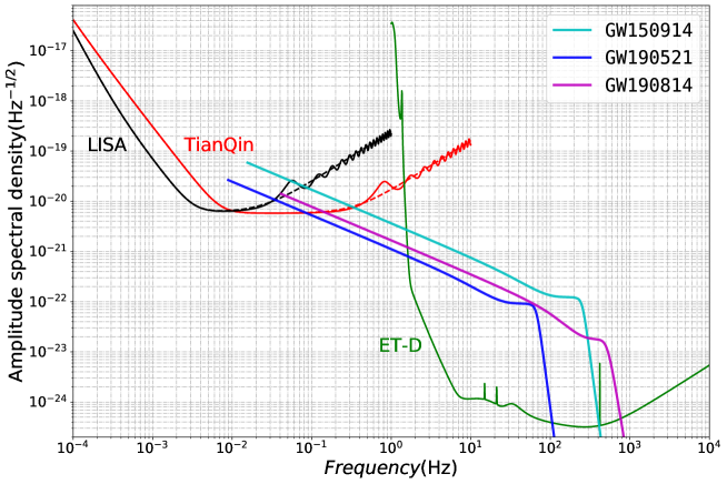
Figure 1: Anticipated sensitivity curves for TianQin (red line), LISA (black line), and ET-D (green line). Additionally, the amplitude spectra densities $\sqrt{f}|\widetilde{h}(f)|$ of GW150914 2016PhRvL.116f1102A (cyan line), GW190521 Abbott:2020tfl (blue line), and GW190814 Abbott:2020khf (magenta line) detected by Advanced LIGO and Virgo, assuming a 5 years merger time.

For a GW source characterized by a parameter set of $\vec{\theta}\equiv(\mathcal{M}_{z},\eta,D_{L},\alpha,\delta,\iota,t_{c},\Psi_{c},\psi)$ detected from multiple independent detectors, the Fisher information matrix (FIM) can provide a Cramér-Rao lower bound on the parameter estimation uncertainty Vallisneri_2008 . The FIM is defined as follows:

$$\Gamma_{mn}\equiv\left\langle\frac{\partial\bm{h}}{\partial\theta_{m}}\bigg{|}\frac{\partial\bm{h}}{\partial\theta_{n}}\right\rangle=\sum_{k}\left\langle\frac{\partial h_{k}}{\partial\theta_{m}}\bigg{|}\frac{\partial h_{k}}{\partial\theta_{n}}\right\rangle,$$ (19)

where $\theta_{m}$ indicates the $m$-th parameter of the GW event. The covariance matrix $\Sigma$ equal to the inverse of the FIM, $\Sigma=\Gamma^{-1}$, we can adopt $\Delta\theta_{m}=\sqrt{\Sigma_{mm}}=\sqrt{(\Gamma^{-1})_{mm}}$ as the estimation error of the parameter, with the sky localization error being $\Delta\Omega=2\pi|\sin\delta|\sqrt{\Sigma_{\alpha\alpha}\Sigma_{\delta\delta}-\Sigma_{\alpha\delta}^{2}}$.

II.4 Galaxy weighting

Assuming that the formation rate of the SBBH per unit stellar mass is uniform across all galaxies, we can expect that the probability of a galaxy hosting the SBBH is proportional to its total stellar mass.

The $K$-band luminosity is a commonly used parameter to account for the galaxy’s mass. The $K$-band is commonly accepted to trace the galaxy’s old stellar population and, thus, is approximately proportional to the galaxy’s stellar mass, as well as being weakly correlated with the galaxy’s color Bell:2003cj ; Lin:2004ak . Following this logic, the $K$-band luminosity weighting method was applied to the dark standard siren cosmological analysis using LIGO&Virgo data Fishbach:2018gjp ; Gray:2019ksv ; Abbott:2019yzh .

In this work, we aim to adopt a different approach to improve the galaxy weighting process in order to obtain more accurate cosmological parameter estimation. This is achieved by deriving the galaxy’s stellar masses from the multi-band photometry of the galaxy samples.

II.4.1 Galaxy sample and the completeness of the catalog

We use the Gravitational Wave Events in Sloan (GWENS) galaxy catalog Rahman:2019 ; Abbott:2019yzh , which has been assembled on purpose for the EM-GW multimessenger observations. It uses the Sloan Digital Sky Survey (SDSS) Data Release 14 (DR14) Abolfathi:2017vfu , which maps over $45$ million galaxies, covering about a quarter of the whole sky. The GWENS catalog provides photometric information in five bands of $ugriz$ for all galaxies, corresponding to cModel magnitudes (see SDSS DR14 paper Abolfathi:2017vfu ) corrected for Galactic extinction from Schlegel:1997yv . Additionally, the GWENS catalog contains photometric redshifts (photo-$z$) for the majority of the sample (about $98.5\%$) and spectroscopic redshifts for a small portion.

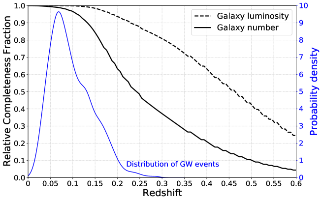
Figure 2: The solid and dashed black lines represent completeness fractions of the GWENS catalog relative to local values, in terms of number and luminosity (in $z$-band), respectively. The blue line represents the probability distribution of simulated detectable GW events, with the scales shown on the right side.

The completeness of a galaxy catalog plays a vital role in the dark standard of siren study. FIG. 2 shows the relative completeness fraction of the GWENS catalog at different redshifts. This is obtained by using the galaxy luminosity distribution within $z<0.05$ as the fiducial distribution, assuming that galaxies are distributed uniformly in the co-moving volume, and neglecting the evolution of the galaxy luminosity distribution with redshift. According to previous GW forecast studies (Liu:2020eko, ) conclude that the SBBH inspirals detectable by TianQin are mainly concentrated in the $z<0.2$, region with the highest redshift not exceeding $z=0.3$. The GWENS catalog has a relative completeness fraction of around $0.63$ at $z=0.2$ and $0.37$ at $z=0.3$ in terms of the number of galaxies; however, in terms of the total luminosity contributed by galaxies, the relative completeness fraction remains above $0.9$ at $z=0.2$ and equal to or greater than $0.8$ at $z=0.3$. These levels of relative completeness ensure that the majority of host galaxies for GW sources are included in the list, and the GWENS catalog meets our requirements. There exist other galaxy catalogs available, such as the GLADE catalog Dalya:2018cnd and the DES catalog Abbott:2021hoj ; Drlica-Wagner:2017tkk ; Abbott:2018jhe ; however, we chose the GWENS catalog due to its higher completeness and broader sky coverage.

II.4.2 Stellar masses

Galaxy masses are calculated using Le Phare, a widely used spectral energy distribution (SED) fitting software Arnouts:1999bb ; Ilbert:2006dp . Le Phare matches observed galaxy colors to predicted colors using a set of theoretical SED libraries derived from simple stellar population models, characterized by a series of stellar parameters such as age $\tau$, metallicity $Z$, and a star formation history. The SED is convolved with the filter transmission curves (including instrument efficiency) adopted for the specific observation dataset in order to provide synthetic luminosities in the chosen bands. The best-fit parameters are obtained via minimizing the $\chi^{2}$ difference between the synthetic color SED and the photometric data. The input data set is made up of multi-band photometric magnitudes from the GWENS catalog Rahman:2019 ; Abbott:2019yzh . The output data set consists of the best stellar population parameters, such as age, metallicity, rate of star formation, and stellar mass. We adopt stellar templates from Bruzual:2003tq in the simple stellar population models, together with an initial mass function from Chabrier:2003ki and an exponentially decaying star formation history. We use a diverse collection of models with three metallicities ($0.005Z_{\odot}$, $Z_{\odot}$, and $2.5Z_{\odot}$) and different ages (${\tau}\leq{\tau}_{\rm max}$), with the maximum age ${\tau}_{\rm max}$, set by the age of the Universe at the redshift of the galaxy, with a maximum value at $z=0$ of $13.5\ \rm Gyr$. We also consider internal extinction using the models from Calzetti:1994vw . Finally, in the Le Phare run, we fix the galaxy redshift to the median of the probability density function of photo-$z$ reported in the GWENS catalog to reduce degeneracies between redshift and galaxy colors. FIG. 3 shows the final distribution of stellar masses for the $45\,141\,307$ GWENS galaxies. The stellar masses range, from dwarf-like systems ($\sim 10^{7}M_{\odot}$) to massive galaxies ($\sim 10^{12}$), as do the redshifts (from $z=0$ to $z\sim 0.8$).

To check the presence of biases in our mass estimates, we compare them to those obtained for SDSS DR 12 (Portsmouth SED-fit Stellar Masses, which is a catalog of stellar masses of $1\,489\,670$ systems from the Portsmouth Group , see also Maraston:2012jf ), for which we have discovered an overlap of $\sim 53\,700$ galaxies with GWENS. The mean deviation between our estimates and the SDSS “starburst model” catalog is $\Delta_{M}=0.14$ and the scatter $\sigma_{M}=0.32$ in logarithmic space, meaning that the two stellar mass estimates are basically consistent with each other (note that in the case we compared against the Portsmouth passive model catalog, we obtained a $\Delta_{M}=-0.07$ and scatter $\sigma_{M}=0.18$). The scatter obtained by these comparisons is quite small considering the two approaches’ rather different models (e.g., Maraston:2004em and Maraston:2008nn templates, no reddening, and a different magnitude definition).

Figure 3: Distribution of total stellar masses for GWENS galaxies derived from the Le Phare software. Note that the redshift in horizontal coordinates represents the median of the posterior probability distribution of the photo-$z$ of galaxies.

III Simulations

To perform a quantitative analysis of the Hubble constant constraint imposed by GW signals using future space-borne and ground-based GW detectors, we first simulate a GW event catalog, then identify candidate host galaxies according to the spatial localization of the GW source, and finally obtain their statistical redshift information.

III.1 Stellar-mass black hole binary signals

We adopt the “Power Law + Peak” model to populate the SBBH simulation LIGOScientific:2020kqk . Based on the 50 GW events published by the first (GWTC-1) LIGOScientific:2018mvr and the second Gravitational-Wave Transient Catalog (GWTC-2) Abbott:2020niy , this mode has been associated with the highest Bayesian factor LIGOScientific:2020kqk . The model includes a power-law mass distribution for the primary component, with a smooth truncation at the lower mass limit and a Gaussian peak at the high mass end to account for the pile-up effect of pulsational pair-instability supernovae LIGOScientific:2020kqk ; Talbot:2018cva . The mass ratio $q$, which describes the ratio between the secondary component mass and the primary component mass, is modeled by a power law LIGOScientific:2018jsj ; Roulet:2018jbe ; Fishbach:2019bbm , $p(q|m_{1})\propto q^{\beta_{q}}$, and $\beta_{q}=1.3_{-1.6}^{+2.4}$ LIGOScientific:2020kqk . According to LIGOScientific:2020kqk , we adopt the associated SBBH merger rate as $R_{\rm SBBH}=58_{-29}^{+54}\ {\rm Gpc}^{-3}{\rm yr}^{-1}$ , which assumes that $m_{1}\geq 2M_{\odot}$ and includes GW190814.

Moreover, we ignore the spins of inspiralling SBBHs because the black hole spin effect has a negligible effect on the GW cosmology study Mangiagli:2018kpu ; Nishizawa:2016jji . The eccentricity of the SBBH, which is not well constrained by LIGO and Virgo observations, should have non-negligible effects on space-borne GW detections. Throughout this work, we set the eccentricity to $e_{0}=0.01$ at GW frequency equal to $0.01$ Hz as a representative value Nishizawa:2016jji ; Liu:2020eko .

Furthermore, we assume that SBBHs are uniformly distributed in the co-moving volume. Each GW event is hosted randomly in a galaxy from the GWENS catalog, assuming that the probability of each galaxy being hosted by a GW event is proportional to its total stellar mass. The orientation parameter distribution is chosen to be isotropic, i.e., $\alpha\in\textrm{U}[0,2\pi]$, $\cos\delta\in\textrm{U}[-1,1]$, $\alpha_{L}\in\textrm{U}[0,2\pi]$, and $\cos\delta_{L}\in\textrm{U}[-1,1]$; the spins are fixed at $\chi_{1,2}\equiv 0$; the remaining parameters are assumed to obey uniform distribution, $t_{c}\in\textrm{U}[0,20]\ \rm yr$, and $\Phi_{c}\in\textrm{U}[0,2\pi]$. Finally, we produce the simulated GW signals with the IMRPhenomPv2 waveform Hannam:2014 .

III.2 Detections with GW detectors

In this work, we investigate different detector configurations, including those using space-borne and ground-based GW detectors, as described below,

• TianQin: the default situation in which three satellites form a constellation and operate in a “3 months on + 3 months off” mode, with a mission life time of 5 years Luo:2015ght ;

• TianQin I+II: twin constellations of satellites with perpendicular orbital planes, that operates in a relay mode and can avoid the 3 months gap in data Wang:2019 ; Liu:2020eko ; Liang:2021bde ;

• TianQin+LISA: a multi-detector GW detector network of TianQin and LISA, we adopt LISA configuration according to LISA:2017pwj ; Robson:2019 , and considering 4 years of overlap in operation time;

• TianQin I+II+LISA: similar to above but with the TianQin I+II configuration considered;

• TianQin+ET: a multi-band GW detector network of TianQin and ET, with 5 years of overlap in operation time, we adopt ET configuration according to Punturo:2010zz ; Hild:2010id ; Maggiore:2019uih , and assume they will continue operating for 15 years after the end of the TianQin mission;

• TianQin I+II+ET: similar to TianQin+ET but with the TianQin I+II configuration considered.

In TABLE I, we list the anticipated detection rates with respect to different detection thresholds for SBBH inspirals that merge within $20$ years from the start of TianQin detection. Throughout this work, we adopt two SNR thresholds for different detector configurations, one with $\rho_{\rm thre}=8$ for space-borne GW detectors Liu:2020eko ; Kyutoku:2016ppx , including TianQin, TianQin I+II, TianQin+LISA, and TianQin I+II+LISA; and the other with $\rho_{\rm thre}=5$ for multi-band GW detections Wong:2018uwb ; Ewing:2020brd , such as TianQin+ET and TianQin I+II+ET. It is worth mentioning that, for sources with $\rho\geq 5$ detected with space-borne GW detectors/networks, they can all be detected by ET with $\rho\gtrsim 20$, as long as ET is operating when they merge. Therefore we do not list the detection rate of ET separately in TABLE I, and we do not consider GW sources that can only be detected by ET in this work.

Table I: Total detection rate of the SBBHs with $t_{c}<20\rm yr$ over the entire observation time that based on the “Power Law + Peak” SBBH population model for five detector configurations: TianQin, TianQin I+II, LISA, TianQin+LISA, and TianQin I+II+LISA.

SNR	Total detection rate
Threshold	TianQin	TianQin I+II	LISA	TianQin+LISA	TianQin I+II+LISA
$\rho\geq 5$	$44.2_{-21.1}^{+43.1}$	$111.6_{-53.3}^{+108.1}$	$74.2_{-36.2}^{+70.3}$	$155.9_{-75.7}^{+147.4}$	$245.8_{-120.1}^{+234.9}$
$\rho\geq 8$	$10.8_{-5.5}^{+10.1}$	$28.4_{-14.9}^{+26.0}$	$16.8_{-8.2}^{+16.7}$	$38.3_{-19.4}^{+36.1}$	$63.8_{-32.7}^{+58.7}$
$\rho\geq 12$	$3.0_{-1.4}^{+3.1}$	$7.8_{-3.6}^{+7.8}$	$4.6_{-1.9}^{+4.6}$	$10.6_{-5.2}^{+9.9}$	$17.5_{-8.5}^{+17.6}$

The precision of the Hubble constant constrained by GW signals from SBBHs mainly depends on the spatial localization errors of the GW sources. In FIG. 4, we illustrate the marginalized distribution on relative error of luminosity distance $\sigma_{D_{L}}/D_{L}$ and sky localization $\Delta\Omega$. Due to the fact that GW events are useful for reconstructing the ‘$D_{L}-z$ relation’ only when the luminosity distance can be reasonably estimated, we only include the GW sources with $\sigma_{D_{L}}/D_{L}<0.6$ (approximately corresponding to $\Delta D_{L}/D_{L}<1$ at the confidence level of $90\%$) for consideration in this work.

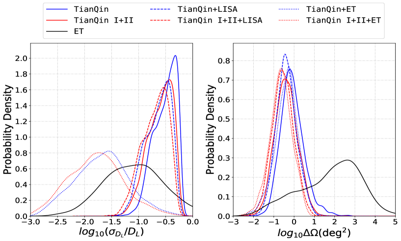
Figure 4: Spatial localization error distribution of TianQin (solid blue line), TianQin I+II (solid red line), TianQin+LISA (dashed blue line), TianQin I+II+LISA (dashed red line), TianQin+ET (dotted blue line), TianQin I+II+ET (dotted red line), and ET (solid black line).

We observe that for events detected by TianQin or TianQin I+II, the relative error of the luminosity distance for most GW sources is greater than $0.1$, but the sky position of most GW sources can be localized to better than $1\ \rm deg^{2}$. The network of TianQin (or TianQin I+II) and LISA can marginally improve the spatial localization of the GW sources. This is because TianQin has better sensitivity than LISA at higher frequencies, which is where the SBBH inspiral signals are concentrated.

On the other hand, for ET-detected events, due to the time-dependent modulation of antenna beam-pattern related to the Earth’s rotation, a typical sky localization error is at the level of $10^{2}\sim 10^{3}\ \rm deg^{2}$. Noting the strong degeneracy between sky localization and luminosity distance, because the polarization angle of a GW signal is dependent on the relative position of the GW source and the detector; such a large sky localization error results in a large uncertainty on polarization, which translates into a large uncertainty on inclination angle and eventually on luminosity distance. Although the majority of GW signals detected by ET have a high SNRs (on the order of $10^{2}\sim 10^{3}$), the typical relative error on the luminosity distance is about $0.1$.

Of course, the multi-band GW cosmology is only meaningful if one can identify the common origin of a binary from both frequency bands. Fortunately, this can be achieved thanks to the excellent parameter recovery ability in either frequency band. Two binary black hole signals that share highly consistent merging time ($\Delta t_{c}\lesssim 1\ {\rm s}$), location ($\Delta\Omega\lesssim 1\ {\rm deg}^{2}$), mass ($\Delta\mathcal{M}_{z}/\mathcal{M}_{z}\sim 10^{-7}$), and distance ($\Delta D_{L}/D_{L}\sim 10^{-1}$) can be easily identified as the same binary Liu:2020eko . Even in the pessimistic scenario that the SNR in TianQin band is too weak for independent detection, the archival search methods Wong:2018uwb ; Moore:2019pke ; Ewing:2020brd can be used to find the signal. Searching for archive data triggered by ET detections is a very practical way to achieve multi-band identification.

One remarkable conclusion we can draw from FIG. 4 is that the multi-band GW detection can significantly improve the estimation precision of the luminosity distance. Accurate GW detection from space-borne detectors can provide very precise sky localization, breaking the degeneracy between sky localization and luminosity distance for ground-based detectors. The relative error on luminosity distance can be improved by one order of magnitude compared with TianQin/LISA and by half an order of magnitude compared with ET.

III.3 Statistical redshift

The spatial localization information of the GW source cannot be directly used to select candidate host galaxies of the GW source. The possible range of luminosity distance $[D_{L}^{-},D_{L}^{+}]\equiv[(\bar{D}_{L}-2\sigma_{D_{L}}),(\bar{D}_{L}+2\sigma_{D_{L}})]$ (where $\bar{D}_{L}$ is the mean value) needs to be converted into the possible range of redshift $[z^{-},z^{+}]$ first. The candidate host galaxies are then selected from the survey galaxy catalog using the redshift-space error box. This conversion depends on both a specific cosmological model and the prior of the corresponding cosmological parameters. We convert the luminosity distance range into the redshift possible range under the standard $\Lambda$CDM model, with the prior of $H_{0}\in{\rm U}[30,120]\ \rm km/s/Mpc$ and $\Omega_{M}\in{\rm U}[0.04,0.6]$. The conversion relation is given by

$$D_{L}^{-} =c(1+z^{-})\int_{0}^{z^{-}}\frac{1}{H^{-}(z^{\prime})}\mathrm{d}z^{\prime},$$ (20a)

$$D_{L}^{+} =c(1+z^{+})\int_{0}^{z^{+}}\frac{1}{H^{+}(z^{\prime})}\mathrm{d}z^{\prime},$$ (20b)

where $H^{-}(z)$ and $H^{+}(z)$ are the specific Hubble parameter realizations that minimize and maximize Eq. (1) within the prior of both $H_{0}$ and $\Omega_{M}$.

In our simulation, we obtain the candidate host galaxies of the GW source from the GWENS catalog. To properly account for the redshift uncertainty, we consider two factors: (1) The redshift information of galaxy in the catalog is almost all photo-$z$, including non-negligible photo-$z$ error $\Delta z_{\rm photo}$; (2) Due to the peculiar velocity of galaxies, the observed spectroscopic redshift $z_{\rm obs}$ is different from the cosmological redshift $z$, and we denote this redshift error $\Delta z_{\rm pv}\equiv|z_{\rm obs}-z|$. In general, $\Delta z_{\rm photo}\gg\Delta z_{\rm pv}$, so the final boundary of the redshift of candidate host galaxies is defined as $[z_{\min},z_{\max}]=[(z^{-}-\Delta z_{\rm photo}),(z^{+}+\Delta z_{\rm photo})]$. The final spatial localization error box of candidate host galaxies is defined by $4\Delta\Omega\times[z_{\min},z_{\max}]$ (the factor of $4$ corresponds to the $2\sigma$ confidence level for the GW sky localization). For a small number of galaxies with spectroscopic redshift, we discard $\Delta z_{\rm photo}$ and approximate $\Delta z_{\rm pv}\approx(1+z_{\rm obs})\langle v_{\rm p}\rangle/c$, assuming $\langle v_{\rm p}\rangle=500\ \rm km/s$ He:2019dhl . The impact of peculiar velocities and their reconstruction on the estimation of $H_{0}$ has been studied in Refs. Howlett:2019mdh ; Nicolaou:2019cip ; He:2019dhl ; Mukherjee:2019qmm , and it is possible to eliminate the redshift error $\Delta z_{\rm pv}$ for nearby galaxies.

To obtain the statistical redshift distributions of GW sources, for each galaxy in the localization error box, we adopt the following two methods:

• fiducial method: assigning equal weight regardless of its position and luminosity;

• weighted method: assigning a weight that accounts for both its positional and luminosity-related information.

When the sky localization from GW detection is described by a covariance matrix $\Sigma_{\alpha\delta}$, the positional weight of a galaxy at location $(\alpha_{j},\delta_{j})$ is defined as $W_{\rm posi}\propto\exp\left\{-\frac{1}{2}\left[\big{(}\alpha_{j}-\bar{\alpha},\delta_{j}-\bar{\delta}\big{)}\Sigma_{\alpha\delta}^{-1}\big{(}\alpha_{j}-\bar{\alpha},\delta_{j}-\bar{\delta}\big{)}^{\rm T}\right]\right\}$, where $(\bar{\alpha},\bar{\delta})$ are the best measured values of the sky localization. Meanwhile, we apply a luminosity-related weight corresponding to total stellar mass of the galaxy, which is derived using multi-band photometric information through the Le Phare software (see Section II.4 for details).

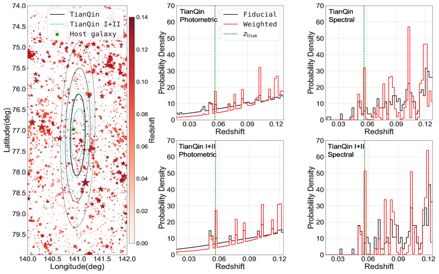
Figure 5: Sky localization and statistical redshift distribution of an example SBBH inspiral. The left panel shows sky localizations of TianQin (solid black contour lines) and TianQin I+II (dashed cyan contour lines), as well as a scatter plot of galaxies within the catalog. The green star labels the real host galaxy; the shade of the star represents its redshift, and the size of the star represents its luminosity-related weight. The center panels show the statistical photo-$z$ of TianQin (top) and TianQin I+II (bottom), respectively, using two different statistical redshift estimations with both the fiducial method (black histograms) and the weighted method (red histograms), and the vertical green dashed line represents the true redshift of the GW source. The right panels show the same as the center panels but with spectroscopic galaxy redshifts.

FIG. 5 illustrates an example localization of a SBBH GW signal and the impact of different weighting methods as well as redshift (photometric or spectroscopic) on the final redshift estimation of the SBBH. While the sky localization of GW source is insufficiently precise to uniquely identify the host galaxy in the absence of an EM counterpart; more accurate sky localization can eliminate the interference of many polluting galaxies. The left panel shows the advantage of the more accurate sky localization of TianQin I+II over TianQin in selecting the galaxies; the middle panels show the different distributions of the statistical redshifts for the two detector configurations. One can conclude that with fewer candidate host galaxies, the true host galaxy’s redshift becomes more significant. Additionally, the distribution of redshift determined by photometric data appears to be more smooth due to large photo-$z$ error, whereas the distribution determined by spectroscopic data shows larger fluctuations, implying a greater potential for constraining the Hubble constant. Notably, because the quality of the statistical redshift distribution for the host galaxy is mainly dependent on the spatial localization precision provided by the GW detection, we do not repeat the above illustration for other configurations where the sky localization is not significantly different.

It is slightly counter-intuitive that improved sky localization would result in a worse redshift estimate. This is because the photo-$z$ estimate for any single galaxy is usually accompanied by a sizeable random error. When the GW signal is localized to a larger area, it involves a greater number of galaxies, and the intrinsic clustering of galaxies effectively averages out the random error. On the other hand, such averaging is less effective for more accurate sky localization. However, we anticipate that future detections will trigger an interest in a comprehensive survey of galaxies within the GW localization error box. Therefore, we expect that for events with a spatial resolution of less than $\Delta\Omega<0.1\ {\rm deg}^{2}$, spectroscopic redshift will be available for galaxies with an apparent magnitude $m_{\rm app}\leq+21\ \rm mag$ Gong:2019yxt . In practice, we simply adopt the median value of the photo-$z$ as the “true value” of the spectroscopic redshift.

IV Results

To extract the Hubble constant from the dark standard sirens, we use a Markov chain Monte Carlo (MCMC) algorithm — emcee package, which is a Python implementation of an affine-invariant MCMC ensemble sampler ForemanMackey:2012ig ; ForemanMackey:2019ig . In FIG. 6, we illustrate how to estimate cosmological parameters using the SBBH GW detections of TianQin I+II. We demonstrate that although a single event may suffer from large uncertainties due to its inability to identify the host galaxy, but a number of events can cancel out the random error and result in a more precise estimate of the Hubble constant.

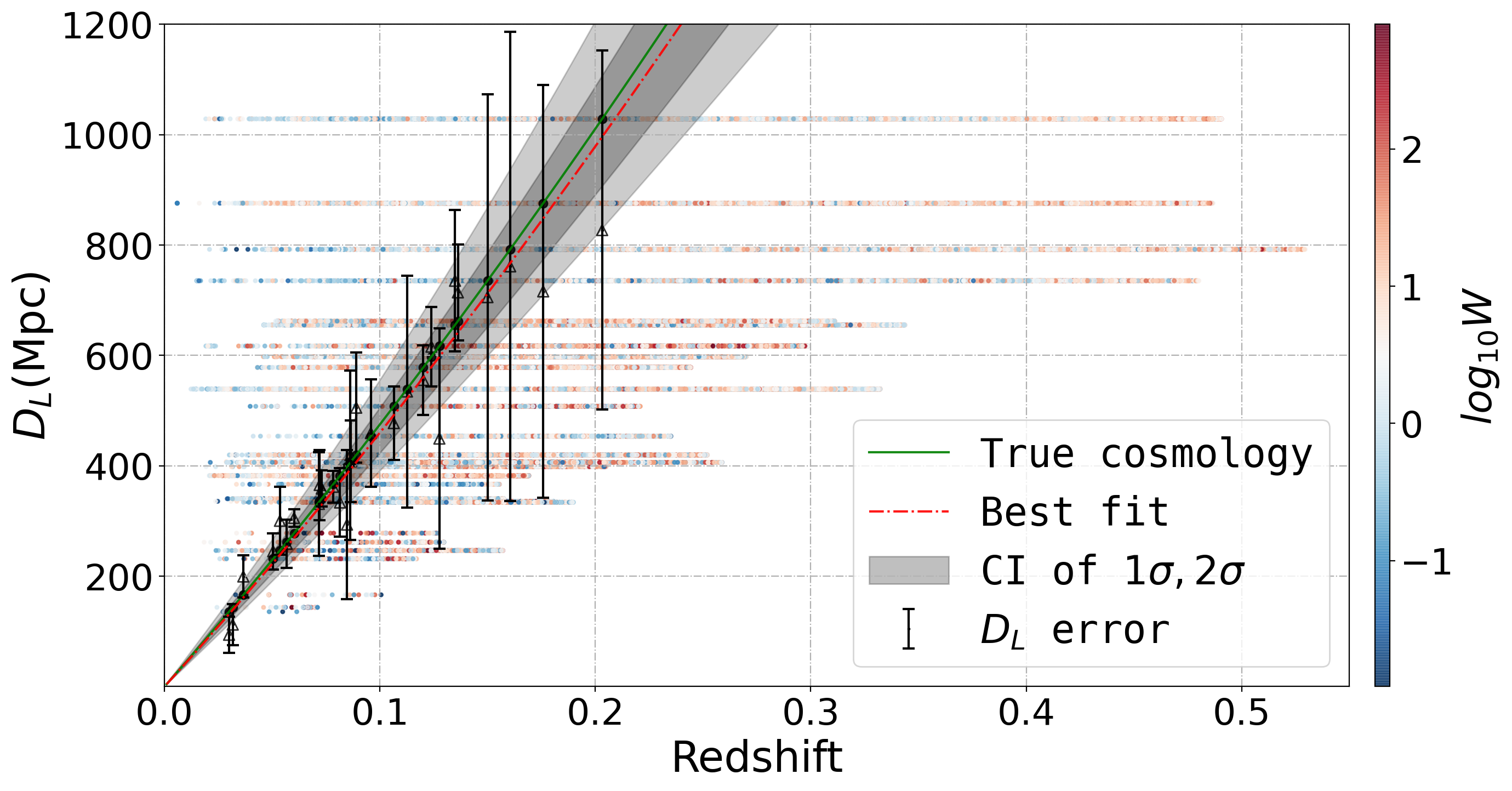
Figure 6: Example of fitting the ‘$D_{L}-z$ relation’ based on the dark standard siren observations of TianQin I+II. The solid green line represents injected cosmological parameters $H_{0}$ and $\Omega_{M}$. The dotted-dashed red line represents the most probable cosmology, while the two shaded areas represent confidence intervals of $68.27\%$ ($1\sigma$) and $95.45\%$ ($2\sigma$), respectively. The black error bars represent measurement errors in determining the luminosity distance to GW sources. The median hollow black triangles in each error bar represent the mean of the $D_{L}$ measurement with random statistical deviation, while the solid black dot represents the true value of $D_{L}$. The horizontal colored dots represent the redshift of selected galaxies for that particular source. The color hues from blue to red show the logarithms of the total weights of galaxies, and we assigned a value to the $D_{L}$ of each candidate host galaxy equal to the true $D_{L}$ of the GW source.

Because of the uncertainty related to the luminosity distance, the redshift ($\Delta z_{\rm photo}$ and $\Delta z_{\rm pv}$), and the cosmological model, a single GW event is frequently associated with a large number of galaxies with a wide range of redshifts (see Eq. (20a, 20b)), which are shown as the horizontally distributed dots in FIG. 6. After constraining cosmological parameters, the redshift range of candidate host galaxies of the GW source will be considerably reduced, which is referred to as posterior redshift. The candidate host galaxies within the posterior redshift range ultimately determine the precision with which cosmological parameters can be estimated. The other candidate host galaxies outside the posterior redshift are just interference sources, and we cannot exclude them when the cosmological parameters are not constrained.

The results of constraints on $H_{0}$ using SBBH GW signals are shown in this section for different detector configurations, including TianQin, TianQin I+II, TianQin+LISA, TianQin I+II+LISA, TianQin+ET, and TianQin I+II+ET. To alleviate the random effect of random realization, we repeat the calculation on 48 random realizations with different random seeds for each configuration and the two weighting methods. Furthermore, when reporting the constraining on $H_{0}$, the result is marginalized over $\Omega_{M}$ instead of being fixed at a specific $\Omega_{M}$ value.

IV.1 TianQin and TianQin I+II

The current studies of the population properties of SBBH merger events observed by LIGO and Virgo have revealed a large uncertainty in the merger rate of SBBHs LIGOScientific:2018mvr ; LIGOScientific:2018jsj ; Abbott:2020niy ; LIGOScientific:2020kqk , which also results in large uncertainty in the prediction of the detection rate of GW events derived from SBBHs. We studied the variation of the constraint precision of $H_{0}$ with the number of GW events in a range of $6$ to $120$ events to avoid the influence of the detection rate of GW events on the constraint precision of $H_{0}$ and fully display the potential of detectors. The constraints on $H_{0}$ for TianQin and TanQin I+II are shown in FIG. 7. The uncertainty of $H_{0}$ shrinks as the number of detected GW events increases. In comparison to the fiducial method, the weighted method can improve the constraining precision of $H_{0}$ by a factor of about $2$.

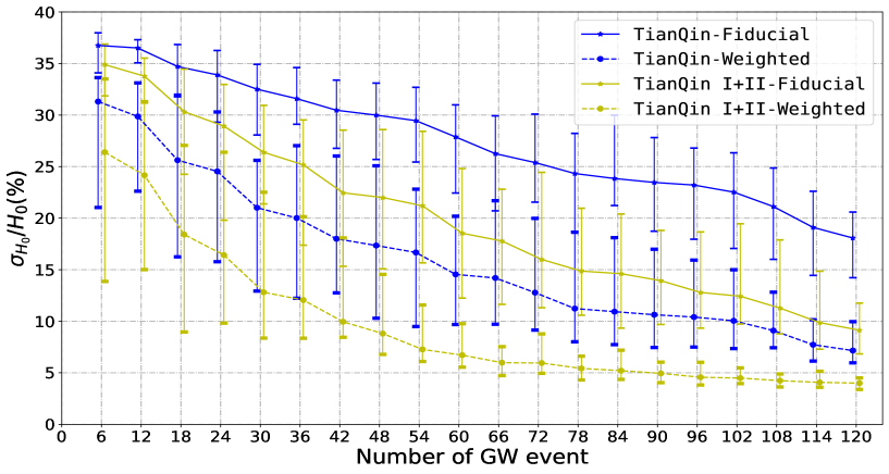
Figure 7: Dependence of constraint precision of $H_{0}$ on the numbers of GW events for TianQin (blue) and TianQin I+II (yellow). The fiducial method and the weighted method are shown in solid and dashed lines, respectively. Each error bar represents a $68.27\%$ interval from 48 independent simulations. The lines have been slightly shifted to improve the visual presentation.

TianQin can detect approximately $11$ SBBH GW events over 5 years of operation (as illustrated in TABLE I), with which one can constrain $H_{0}$ to a precision of approximately $36.8\%$ using the fiducial method and approximately $30.9\%$ using the weighted method, respectively. Due to the small number of GW events, the constraints on cosmological parameters are very imprecise. A typical constraint result of the parameters $h$ ($h\equiv\frac{H_{0}}{100\ {\rm km/s/Mpc}}$) and $\Omega_{M}$ from TianQin using the weighted method is shown in the left plot of FIG. 8.

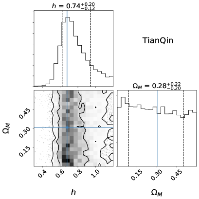
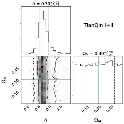
Figure 8: Example posterior probabilities of the parameters $h$ and $\Omega_{M}$ calculated using the weighted method for TianQin (left) and TianQin I+II (right). In each plot, the lower left panel shows the joint posterior probability of $h$ and $\Omega_{M}$, with the contours representing confidence levels of $1\sigma(68.27\%)$ and $2\sigma(95.45\%)$, respectively; the upper and right panels show the marginalized posterior distribution of the same parameters, with the dashed lines indicating a $1\sigma$ credible interval. In each panel, the solid cyan lines mark the true values of the parameters.

The constraint on $H_{0}$ with TianQin I+II is tighter than that with TianQin, as shown in FIG. 7. Given the same number of GW events and the weighting method of candidate host galaxies, TianQin I+II can significantly improve the constraint of $H_{0}$. This improvement is mainly due to the more accurate spatial localization provided by TianQin I+II, as shown in FIG. 4. Using the fiducial method and the weighted method, approximately $28$ GW events are expected to be detected by TianQin I+II, and the precision of $H_{0}$ is expected to be approximately $26.3\%$ and $14.4\%$, respectively. A typical cosmological parameter estimation using the weighted method for TianQin I+II is shown in the right plot of FIG. 8. The non-Gaussian tail of the posterior probability distribution of $H_{0}$ becomes shorter as the rate of GW detection increases and the spatial localization of GW sources becomes more precise. Additionally, when using SBBH GW events, either for TianQin or TianQin I+II, there are no effective constraints on $\Omega_{M}$ parameter.

It is worth noting that the precision of $H_{0}$ estimation with TianQin using the weighted method is higher than that obtained using the fiducial method with TianQin I+II, indicating that in comparison to improved spatial localization, the more accurate weighting method has a larger impact on $H_{0}$ estimation.

IV.2 Multi-detector network of TianQin and LISA

We then analyze scenarios in which LISA is added to the detector network. In FIG. 9, we show the dependence of the precision of $H_{0}$ versus detection numbers, assuming TianQin+LISA and TianQin I+II+LISA. Again we observe that increasing the number of detections results in a more precise $H_{0}$ measurement. In FIG. 10, we give a representative joint posterior probability of $h$ and $\Omega_{M}$ using the weighted method under the expected total detection rates (see TABLE I for details). We notice that TianQin+LISA has very similar constraining power to TianQin I+II because the two detection configurations have very similar localization precisions (see FIG. 4). Meanwhile, TianQin I+II+LISA can reduce uncertainty on $H_{0}$ by half as a result of improved localization. On the other hand, neither of the two detector network configurations, imposes any meaningful constraint on $\Omega_{M}$.

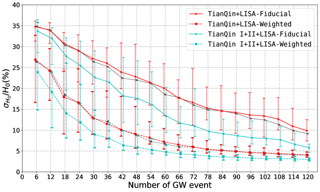
Figure 9: Dependence of constraint precision of $H_{0}$ on the numbers of GW events for TianQin+LISA (red) and TianQin I+II+LISA (cyan). The fiducial method and the weighted method are shown in solid and dashed lines, respectively. Each error bar represents a $68.27\%$ interval generated by 48 independent simulations. For comparison, similar results for TianQin I+II (gray) are also shown. The lines have been slightly shifted to improve the visual presentation.

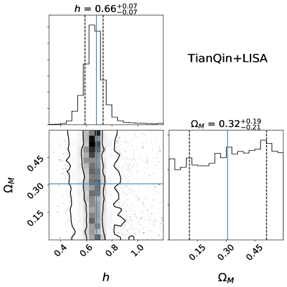
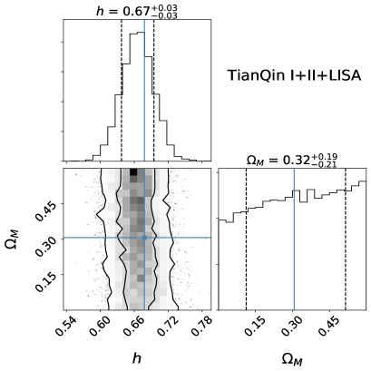
Figure 10: Example posterior probabilities of the parameters $h$ and $\Omega_{M}$ calculated using the weighted method for TianQin+LISA (left) and TianQin I+II+LISA (right). Each plot represents the joint posterior probability of $h$ and $\Omega_{M}$, with contours representing confidence levels of $1\sigma(68.27\%)$ and $2\sigma(95.45\%)$, respectively; the upper show the marginalized posterior distribution of the same parameters, with the dashed lines representing the $1\sigma$ credible interval. In each panel, the solid cyan lines mark the true values of the parameters.

For TianQin+LISA (TianQin I+II+LISA), about $38~{}(64)$ GW events are expected to be detected, and the precision of $H_{0}$ can be constrained to approximately $25.2\%~{}(12.2\%)$ and approximately $11.6\%~{}(4.1\%)$ by using the fiducial method and the weighted method, respectively. Similar to the case of TianQin and TianQin I+II, the constraint of $H_{0}$ by TianQin+LISA using the weighted method is stronger than that by TianQin I+II+LISA using the fiducial method.

Space-borne GW detectors/networks have excellent sky localizing capabilities, which enables the constraints on the Hubble constant through the observation of SBBH inspirals. However, such SBBH inspiral GW signals are relatively quieter; the relatively lower SNR leads to a larger uncertainty on luminosity distance, $\sigma_{D_{L}}/D_{L}\gtrsim 0.1$. This fact limits the expected precision of $H_{0}$ from the SBBH inspiral observation with space-borne detectors.

IV.3 Multi-band detection with TianQin and ET

A multi-band GW observation of SBBHs can significantly improve the constraining on the Hubble constant under the dark standard siren scenario since the multi-band observation combines advantages of both space-borne and ground-based detectors. Space-borne GW detectors can provide accurate sky localization, while ground-based detectors’ high SNR enables more precise luminosity distance estimation. This combination results in a smaller localization error box that is less susceptible to contamination from neighbouring galaxies, resulting in a more precise estimation of the redshift.

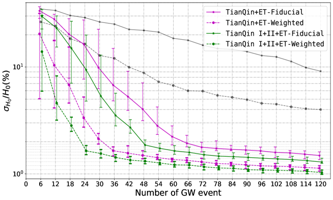
Figure 11: Dependence of constraint precision of $H_{0}$ on the numbers of GW events for TianQin+ET (magenta) and TianQin I+II+LISA (green). The fiducial method and the weighted method are shown in solid and dashed lines, respectively. Each error bar represents a $68.27\%$ interval from 48 independent simulations. Comparable results for TianQin I+II (gray) are also provided. The lines have been slightly shifted to improve the visual presentation.

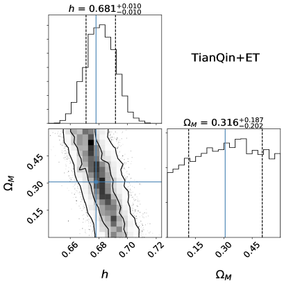
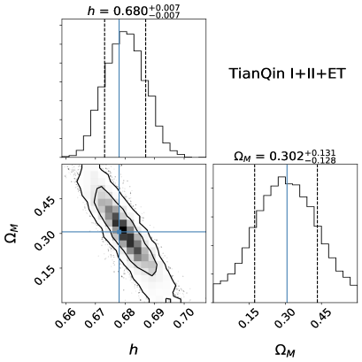
Figure 12: Example posterior probabilities of the parameters $h$ and $\Omega_{M}$ calculated using the weighted method for TianQin+ET (left) and TianQin I+II+ET (right). In each plot, the lower left panel shows the joint posterior probability of $h$ and $\Omega_{M}$, with the contours representing confidence levels of $1\sigma(68.27\%)$ and $2\sigma(95.45\%)$, respectively; the upper and right panels show the marginalized posterior distribution of the same parameters, with the dashed lines indicating a $1\sigma$ credible interval. In each panel, the solid cyan lines mark the true values of the parameters.

In FIG. 11, we present the dependence of constraint precision of $H_{0}$ versus different detection numbers, under the multi-band GW detector networks TianQin+ET and TianQin I+II+ET. Notably, the TianQin I+II lines (gray) approximate a power-law relationship, while the lines for multi-band networks indicate a saturation from relative uncertainties around $1.8\%$, which also corresponds to a turning point for the trend of the lines, respectively. We observe that the multi-band network can quickly increase the precision of $H_{0}$ as more events are observed, but after the turning point, the precision improves only by $1/\sqrt{N}$, where $N$ is the number of GW events. Moreover, the precision is hard to reach the level of $1\%$ even after 100 GW events are detected. Additionally, we notice that when adopting the weighted method, better precision leads to a quicker approach to saturation, which occurs in around 24 events for the TianQin I+II+ET network.

For TianQin+ET, about $44$ GW events are expected to be detected via multiple band observation (as illustrated in TABLE I), and the precision of $H_{0}$ can be constrained to approximately $4.7\%$ and approximately $1.5\%$ by using the fiducial method and the weighted method, respectively. Moreover, if TianQin I+II+ET is realized, approximately $112$ GW events can be detected using multi-band observations in the optimistic case, and the precision of $H_{0}$ can be constrained to $\sim 1\%$, using either the fiducial method (about $1.3\%$) or the weighted method (about $1.1\%$). Constraining $H_{0}$ to a precision of $1\%$ would be very exciting as it has the potential to shed light on the Hubble tension .

The typical constraints on $h$ and $\Omega_{M}$ using the weighted method for the multi-band networks are shown in FIG. 12. The introduction of multi-band GW observation can greatly enhance the constraining power on the cosmological parameter $\Omega_{M}$. While the fiducial method does not deliver significant and robust estimation, the weighted method can constrain $\Omega_{M}$ to a precision of $0.13$, or equivalently $42\%$ for relative uncertainty, with the TianQin I+II+ET network.

V Discussions

V.1 Important role of spectroscopic redshift

Considering that the sky localization error of almost all GW sources is less than $10\ {\rm deg}^{2}$, it may be possible to use current or future spectroscopic observation facilities, such as the Large Sky Area Multi-Object Fiber Spectroscopic Telescope 1998SPIE.3352...76S ; Cui_2012 ; 2012RAA....12..723Z , the Dark Energy Spectroscopic Instrument Aghamousa:2016zmz , the 4-meter Multi-Object Spectroscopic Telescope (4MOST) deJong:2012nj , the TAIPAN daCunha:2017wwy , the Chinese Space Station Telescope Gong:2019yxt , the James Webb Space Telescope Gardner:2006ky ; Kalirai:2018qfg , and the Wide-Field Infrared Survey Telescope Green:2012mj ; Chary:2020msh , to perform galaxy survey and provide accurate estimations of redshifts for the galaxies locate in the error box. In this section, we investigate to what extent a catalog of galaxies with spectroscopic redshifts can improve the constraint precision of $H_{0}$. TABLE II summarizes the constraint precision of $H_{0}$ under various detector configurations and under two assumptions that the survey galaxy catalog with photo-$z$ and with assumed spectroscopic redshift, respectively.

Table II: Expected constraint precision of $H_{0}$ under six detector configures, assuming the survey galaxy catalog with photo-$z$ and with spectroscopic redshift. The error represents $68.27\%$ confidence interval.

Network	Constraint precision $\sigma_{H_{0}}/H_{0}$ (%)
	Using photo-$z$ catalog		Using spectroscopic redshift catalog
configuration	Fiducial method	Weighted method	Fiducial method	Weighted method
TianQin	$36.8_{-1.8}^{+1.7}$	$30.9_{-5.1}^{+5.1}$	$29.7_{-6.2}^{+5.4}$	$22.2_{-9.8}^{+8.3}$
TianQin I+II	$26.3_{-6.9}^{+5.9}$	$14.4_{-7.6}^{+9.4}$	$15.1_{-6.9}^{+9.4}$	$7.9_{-3.2}^{+2.9}$
TianQin+LISA	$25.2_{-7.6}^{+6.4}$	$11.6_{-6.4}^{+8.2}$	$12.4_{-5.4}^{+6.2}$	$6.4_{-2.4}^{+1.6}$
TianQin I+II+LISA	$12.2_{-5.3}^{+5.3}$	$4.1_{-0.8}^{+0.8}$	$5.7_{-2.0}^{+1.5}$	$3.3_{-0.7}^{+0.7}$
TianQin+ET	$4.67_{-1.60}^{+1.80}$	$1.51_{-0.13}^{+0.13}$	$2.10_{-0.63}^{+0.25}$	$1.32_{-0.09}^{+0.10}$
TianQin I+II+ET	$1.32_{-0.09}^{+0.07}$	$1.05_{-0.06}^{+0.05}$	$1.08_{-0.09}^{+0.10}$	$0.95_{-0.08}^{+0.08}$

We observe that the constraint precision of $H_{0}$ is quite low for TianQin. This is because the expected detection rate is low; the detected events are insufficient to suppress random fluctuations, and so the effect of spectroscopic redshift is not significant. However, for a network of detectors, one might anticipate a greater number of detected GW events, which emphasizes the uncertainty associated with the galaxy redshift measurement. We observe that employing spectroscopic redshift can significantly improve the precision of $H_{0}$ by a factor of $2$. However, for TianQin I+II+ET, the saturation described in Section IV.3 allows for extremely exact estimation of $H_{0}$ even without the spectroscopic redshift. But still, by using the weighted method and the spectroscopic redshift, one can expect the $H_{0}$ to be constrained to a level better than $1\%$.

V.2 Information gained from multiple band photometry information

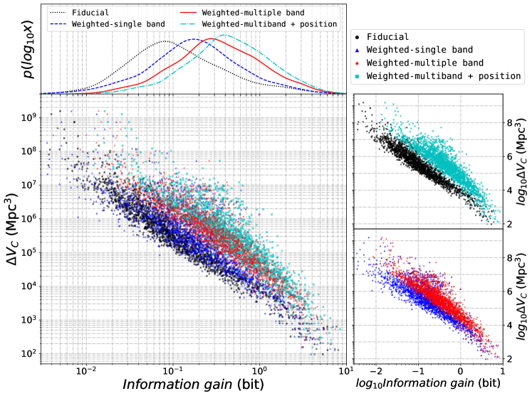
Figure 13: Distribution of statistical redshift information gains for various weighting methods. The black, blue, red, and cyan dots or lines represent the results obtained by the fiducial method, single-band luminosity weighting, multiple band luminosities weighting, and the position plus multi-band luminosity weighting methods, respectively. This figure contains 2000 mock GW events detected from TianQin. The top panel shows the distribution of information gains obtained using these four methods, the bottom left panel shows the scatter distribution of information gain $-$ localization co-moving volume of candidate host galaxies $(\Delta V_{C})$, the right panels decompose the scatters for better distinction.

The use of multi-band luminosity can aid in our comprehension of the redshift information. In this paper, we quantify the role of the multi-band luminosity information in this process. For different weighting scenarios, we calculate the information gain of statistical redshift distributions on top of the prior distribution. The information gain is defined as Sivia:2006book

$$\mathcal{H}=\int p(z|d_{\rm GW},d_{\rm survey},\vec{H},I)\log_{2}\left[\frac{p(z|d_{\rm GW},d_{\rm survey},\vec{H},I)}{p_{c}(z|\vec{H},I)}\right]\mathrm{d}z,$$ (21)

where $p(z|d_{\rm GW},d_{\rm survey},\vec{H},I)$ represents the posterior of redshift for candidate host galaxies of GW sources, $d_{\rm survey}$ represents data of galaxy survey, and $p_{c}(z|\vec{H},I)$ is the prior distribution on redshift, which is defined by Eq. (11).

We illustrate the information gains on statistical redshift in FIG. 13, for four weighting methods: (1) the fiducial method, (2) single-band luminosity weighting method, (3) multiple band luminosities weighting method, and (4) position plus multi-band luminosity weighting method. A total of 2000 mock GW events are used. As can be shown, all methods yield a greater information gain when the localization error is smaller. With more information (in terms of luminosity and position), more information about statistical redshift can be gained. The peak of the marginalized distribution (shown on the top panel) demonstrates that for the four methods, each step provides an information gain increase of roughly 0.1 bits. Moreover, the information gain from the single-band luminosity weighting method is approximately the same for any of the five bands of $ugriz$. In most cases, the weighting method of using both location and multi-band luminosities can yield an information gain of as high as about 0.5 bits.

V.3 Potential to address the Hubble tension

Astronomers are puzzled by the Hubble tension, which describes the inconsistency between the two typical Hubble constant measurement methods, reported as $74.03\pm 1.42\ {\rm km/s/Mpc}$ from SNe Ia observations Riess:2019cxk (also see Ref. Riess:2020fzl ) and $67.4\pm 0.5\ {\rm km/s/Mpc}$ from the $Planck$ CMB anisotropies measurements Planck:2018vyg . Both methods have remarkable accuracies of approximately $1.9\%$ and $0.7\%$, respectively. GW cosmology with dark standard sirens provides a fascinating new means of potentially explaining or resolving the Hubble tension, as it is expected to be much less impacted by systematic errors. However, an equally accurate measurement would be required to achieve so. With the TianQin detectors, even in the most optimal scenario where we assume TianQin I+II with the weighted method and a galaxy catalog with spectroscopic redshift, the estimated precision of $H_{0}$ can only reach $7.9\%$. When LISA is included, the precision can reach the level of $3.3\%$.

On the other hand, a multi-band GW detector network has a very prominent potential to estimate $H_{0}$ accurately. One can expect an $H_{0}$ precision of $1.51\%$ and $1.05\%$ for TianQin+ET and TianQin I+II+ET, respectively, which is very promising for addressing, or at the very least, shedding light on the nature of the Hubble tension.

According to some studies suggest that the multi-detector GW detections of MBHB mergers can also achieve precision close to (or even better than) $1\%$ for $H_{0}$ measurement. This level of precision is typically facilitated by the fact that the MBHB mergers may be registered with a very high SNR using space-borne GW missions Klein:2015hvg ; Holz:2005df ; Wang:2019 ; Feng:2019wgq ; Ruan:2020smc ; Ruan:2019tje . Meanwhile, since MBHB mergers may be detected at a very long distance, they may also be used to recover additional cosmological parameters in addition to $H_{0}$. However, the precision of $H_{0}$ with MBHB detections is highly sensitive to the detection of neighboring events, which usually have a very low detection rate; the high precision is not guaranteed Zhu:2021aat ; Wang:2020dkc . On the other hand, the higher detection rate of SBBHs indicates a highly likely prospect of using their inspiral GW signals to constrain $H_{0}$ with high precision.

V.4 P$-$P plot check

To compensate for the selection effect of galaxies observations, we adopt a correction factor in Eq. (12) with the goal of obtaining an unbiased estimate of the Hubble constant. We want to examine whether the conclusion is indeed unbiased, using both the weighted method and the fiducial method. To do this, we perform a series of P$-$P plots to ensure consistency, as shown in FIG. 14. The horizontal axis shows the credible level, while the vertical axis shows the fraction of simulations in which the true parameters are located within a certain credible interval. For a fully consistent method, we expect the P$-$P plot to be alongside the diagonal line, with some degree of random fluctuations. For a more straightforward comparison, we perform Kolmogorov-Smirnov tests for different lines versus the diagonal line and present the calculated $p$-value in TABLE III, with a larger $p$-value representing better consistency.

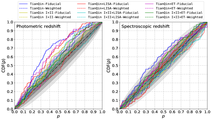
Figure 14: P$-$P plot over $96$ independent simulations on the estimation of the Hubble constant for various detector configurations. The $p$ on the $x$ axis is the credible level, and the CDF$(p)$ (cumulative distribution function, CDF) on the $y$ axis is the fraction of simulations with true parameters within the credible interval. Results with different configurations are shown in different colors, with the fiducial method, the weighted method, and the diagonal line shown in solid, dashed, and dotted-dashed lines, respectively. Different gray shadows represent $1\sigma$, $2\sigma$, and $3\sigma$ confidence intervals, respectively. The left panel makes the assumption that galaxies have photo-$z$ whereas the right panel makes the assumption that spectroscopic redshift is available.

In the left panel, assuming that just photo-$z$ is available for the galaxies, the majority of the solid lines (or the fiducial method) deviate significantly from the diagonal, with a general pessimistic tendency. This is because the posterior probability of the cosmological parameters using the fiducial method does not gain sufficient redshift information from a large number of candidate host galaxies, resulting in a large credible interval, but the true value has most likely already been enclosed. We observe, on the other hand, that the result from the weighted method (dashed lines) is more consistent with the diagonal line, fluctuating well within the $3\sigma$ confidence interval, which indicates a successful implementation of an unbiased estimator for the Hubble constant.

Table III: Meta $p$-value of the distribution of $H_{0}$ estimations obtained from multiple independent simulations under various detector configurations, in comparison to an expected uniform distribution over $[0,1]$. The null hypothesis is set so that the two distributions are consistent; therefore, a $p$-value less than $0.05$ indicates that the simulation results deviate significantly from the ideal result.

Detector	$p$-value
	Using photo-$z$ catalog		Using spectroscopic redshift catalog
configuration	Fiducial method	Weighted method	Fiducial method	Weighted method
TianQin	$5.6\times 10^{-9}$	$0.0756$	$9.8\times 10^{-3}$	$0.3756$
TianQin I+II	$3.8\times 10^{-3}$	$0.2511$	$0.1774$	$0.5081$
TianQin+LISA	$2.3\times 10^{-5}$	$0.2513$	$0.2026$	$0.2419$
TianQin I+II+LISA	$1.9\times 10^{-3}$	$0.6767$	$0.1549$	$0.4871$
TianQin+ET	$2.6\times 10^{-3}$	$0.1085$	$0.1030$	$0.2690$
TianQin I+II+ET	$0.0209$	$0.4074$	$0.2386$	$0.5599$

If galaxies have spectroscopic redshifts, both methods’ P$-$P plots are statistically consistent with the diagonal for all configurations. This finding emphasizes the importance of accurate measurement of galaxy redshifts in estimating the Hubble constant.

V.5 Effect of eccentricity on multi-band GW detection

In this work, we focus on GW sources with very small eccentricities ($e_{0}=0.01$ at $0.01$Hz). This is a reasonable assumption for binary black holes generated via an isolated binary channel, as the GW radiation is expected to circularize the orbit. However, if the SBBHs have a dynamical origin, they may retain higher eccentricities in the millihertz range OLeary:2005vqo ; Kremer:2018tzm , which may affect the multi-band GW detection Barack:2003fp ; Chen:2017gfm ; Randall:2019znp . Indeed, the observations of GW190521 by LIGO and Virgo may suggest such a possibility Abbott:2020tfl ; Gayathri:2020coq ; Gayathri:2020fbl . For extreme eccentricities, the GW signals in the millihertz band may fall below the sensitivity of space-borne GW detectors Chen:2017gfm . Fortunately, the majority of SBBHs are not expected to be associated with extreme eccentricities Nishizawa:2016jji ; Samsing:2018isx , and the general conclusion of our study should not be altered by the inclusion of eccentricities.

V.6 Other potential sources of constraint bias on the Hubble constant

Numerous factors can introduce bias into the estimation of the Hubble constant. We describe the potential sources of the bias in this work as follows.

• The detectable SBBH sources are primarily distributed in the $z\lesssim 0.2$, where Hubble’s law can be used to approximate the expansion of the Universe. Therefore, in the majority of cases, the model-dependent $\Omega_{M}$ has no effect on the outcomes of our $H_{0}$ analysis results. However, a small number of GW events with $z\gtrsim 0.2$ show a certain constraint ability on $\Omega_{M}$, such as the constraint results of TianQin+ET and TianQin I+II+ET. This implies that the cosmological model will introduce a bias when using higher redshift SBBH events to constrain $H_{0}$ with high precision.

• In the GW event catalog simulation, the GW sources are randomly assigned to one of the galaxies in the survey galaxy catalog. However, the survey galaxy catalog may not contain the true host galaxy of the GW source in the actual $H0$ estimation due to the selection effect such as the Malmquist bias. The absence of the true redshift of the GW source in the statistical redshift may also introduce a bias into the estimation of $H_{0}$.

• In the simulation setup, we use the median of photo-$z$ estimation as the true cosmological redshift of the galaxy. However, the actual photo-$z$ measurements have an intrinsic scatter and deviation in relation to the spectroscopic redshifts Abazajian:2008wr ; Abolfathi:2017vfu ; Drlica-Wagner:2017tkk ; DeVicente:2015kyp .

• If some of the detected SBBHs have a primordial black hole genesis, DeLuca:2020qqa ; Clesse:2020ghq ; DeLuca:2020sae ; DeLuca:2021wjr ; Deng:2021ezy , the concept of a host galaxy may lose relevance. Furthermore, drawing conclusions based on the assumption that all SBBHs are produced astronomically may be deceptive.

Of course, there are methods to alleviate the bias. For example, the bias of $H_{0}$ caused by the cosmological model can be avoided by fitting model-independent high-order expansion of the ‘$D_{L}-z$ relation’ Visser:2003vq ; Gong:2004sd , or using the model-independent parameter estimation method such as Gaussian processes Seikel:2012uu ; Cai:2016sby ; Li:2019nux . The selection effect in the catalog of the galaxy survey can be corrected by conducting a follow-up deeper field galaxy survey triggered by the GW detection Bartos:2014spa ; Chen:2015nlv ; Klingler:2019fbl , utilizing both ground-based DES:2005dhi ; Sevilla-Noarbe:2020jpu and space telescopes Gong:2019yxt ; Green:2012mj . By performing a follow-up spectroscopic measurement, the bias introduced by photo-$z$ can be eliminated. Although the possibility of contamination by primordial black holes requires additional investigation, an internal consistency check as introduced in Petiteau:2011we ; Zhu:2021aat may help in identifying and removing the anomaly.

VI Conclusions and Outlook

In this work, we investigate the potential of using SBBH GW events (assuming the “Power Law + Peak” model) observed by space-borne GW detectors as dark standard sirens to constrain the Hubble constant. Several different detection scenarios are considered, for instance, single detectors, such as TianQin and TianQin I+II; multiple detector networks, such as TianQin+LISA and TianQin I+II+LISA; and multi-band GW detector network, such as TianQin+ET and TianQin I+II+ET. The redshift information is obtained statistically from the photometric survey galaxy catalog by matching the sky localization and possible redshift range of the SBBH sources with the position and redshift of galaxies (we adopt the GWENS catalog in this work). Two methods are used to assign the weight of galaxies, including the fiducial method, in which each galaxy within the error box has a uniform weight, and the weighted method, in which the weight of a galaxy is proportional to the total stellar mass of the galaxy derived from the multi-band luminosity through the Le Phare method.

In comparison to single detector detection, both multi-detector networks and multi-band GW observations can significantly improve detection rates and spatial localization. As compared to the fiducial method, the weighted method can significantly improve the constraint precision of the Hubble constant. Using the fiducial method and the weighted method, in the TianQin scenario, the constraint precision of $H_{0}$ is expected to be approximately $36.8\%$ and approximately $30.9\%$, respectively; in the TianQin I+II detection scenario, the precision of $H_{0}$ is expected to be approximately $26.3\%$ and approximately $14.4\%$, respectively. Using the weighted method, the constraint precision of $H_{0}$ in the TianQin+LISA and TianQin I+II+LISA detection scenarios is expected to be approximately $11.6\%$ and approximately $4.1\%$ respectively. In the multi-band GW detection scenarios, the precision of the $H_{0}$ constrain by using the weighted method can approach around $1.5\%$ and $1.1\%$ under TianQin+ET configuration and TianQin I+II+ET configuration, respectively. It should be emphasized that both the weighted method and the multi-band GW detection significantly improve the constraint of $H_{0}$.

Apart from $H_{0}$, the space-borne GW detector can hardly constrain any other cosmological parameter, such as $\Omega_{M}$, through the detections of SBBH inspiral GW signals. However, other cosmological parameters can be constrained by other types of GW sources, such as MBHB mergers Petiteau:2011we ; Tamanini:2016zlh ; Zhu:2021aat . MBHB sources generally have a very high SNRs, and their event horizons can extend to high redshifts ($z\gg 1$). As a result, combining SBBH and MBHB GW observations enables a more thorough analysis of GW cosmology study.

Additionally, we study the extent to which spectroscopic redshift information improves the constraining power of the Hubble constant, which increases not just the precision of the Hubble constant but also the accuracy of the constraint. Finally, we evaluated the reliability of our Bayesian analysis framework and galaxy weighting method using the P$-$P plot method by performing a consistency test.

Certain concerns remain unresolved for future studies, such as incorporating a complete frequency response Zhang:2020khm or the time-delay interferometry response Zhang:2019oet . MCMC can also be used in place of the FIM method to obtain more realistic GW parameter estimations Toubiana:2020cqv . The calibration uncertainty of the laser interferometer on the ground-based GW detector might result in systematic errors in the luminosity distance measurement Karki:2016pht ; Sun:2020wke ; Estevez:2020pvj , such as for ET. We reserve such issues for future investigations.

- [1] Bernard F. Schutz. Determining the Hubble Constant from Gravitational Wave Observations. Nature, 323:310--311, 1986.
- [2] P. A. R. Ade et al. Planck 2015 results. XIII. Cosmological parameters. Astron. Astrophys., 594:A13, 2016.
- [3] N. Aghanim et al. Planck 2018 results. VI. Cosmological parameters. Astron. Astrophys., 641:A6, 2020. [Erratum: Astron.Astrophys. 652, C4 (2021)].
- [4] Wendy L. Freedman. Cosmology at a Crossroads. Nature Astron., 1:0121, 2017.
- [5] Wendy L. Freedman, Barry F. Madore, Dylan Hatt, Taylor J. Hoyt, In Sung Jang, Rachael L. Beaton, Christopher R. Burns, Myung Gyoon Lee, Andrew J. Monson, Jillian R. Neeley, M. M. Phillips, Jeffrey A. Rich, and Mark Seibert. The carnegie-chicago hubble program. VIII. an independent determination of the hubble constant based on the tip of the red giant branch. The Astrophysical Journal, 882(1):34, aug 2019.
- [6] Wendy L. Freedman. Measurements of the Hubble Constant: Tensions in Perspective. 6 2021.
- [7] Adam G. Riess, Stefano Casertano, Wenlong Yuan, Lucas M. Macri, and Dan Scolnic. Large Magellanic Cloud Cepheid Standards Provide a 1% Foundation for the Determination of the Hubble Constant and Stronger Evidence for Physics beyond CDM. Astrophys. J., 876(1):85, 2019.
- [8] Adam G. Riess. The Expansion of the Universe is Faster than Expected. Nature Rev. Phys., 2(1):10--12, 2019.
- [9] Adam G. Riess, Stefano Casertano, Wenlong Yuan, J. Bradley Bowers, Lucas Macri, Joel C. Zinn, and Dan Scolnic. Cosmic Distances Calibrated to 1% Precision with Gaia EDR3 Parallaxes and Hubble Space Telescope Photometry of 75 Milky Way Cepheids Confirm Tension with CDM. Astrophys. J. Lett., 908(1):L6, 2021.
- [10] Hsin-Yu Chen, Maya Fishbach, and Daniel E. Holz. A two per cent Hubble constant measurement from standard sirens within five years. Nature, 562(7728):545--547, 2018.
- [11] Stephen M. Feeney, Hiranya V. Peiris, Andrew R. Williamson, Samaya M. Nissanke, Daniel J. Mortlock, Justin Alsing, and Dan Scolnic. Prospects for resolving the Hubble constant tension with standard sirens. Phys. Rev. Lett., 122(6):061105, 2019.
- [12] Ssohrab Borhanian, Arnab Dhani, Anuradha Gupta, K. G. Arun, and B. S. Sathyaprakash. Dark Sirens to Resolve the Hubble–Lemaître Tension. Astrophys. J. Lett., 905(2):L28, 2020.
- [13] Ligong Bian et al. The Gravitational-Wave Physics II: Progress. Sci. China Phys. Mech. Astron., 64:120401, 2021.
- [14] B. P. Abbott, R. Abbott, T. D. Abbott, M. R. Abernathy, F. Acernese, K. Ackley, C. Adams, T. Adams, P. Addesso, R. X. Adhikari, and et al. Observation of Gravitational Waves from a Binary Black Hole Merger. Phys. Rev. Lett., 116(6):061102, February 2016.
- [15] B. P. Abbott, R. Abbott, T. D. Abbott, M. R. Abernathy, F. Acernese, K. Ackley, C. Adams, T. Adams, P. Addesso, R. X. Adhikari, and et al. GW151226: Observation of Gravitational Waves from a 22-Solar-Mass Binary Black Hole Coalescence. Phys. Rev. Lett., 116(24):241103, June 2016.
- [16] B. P. Abbott, R. Abbott, T. D. Abbott, F. Acernese, K. Ackley, C. Adams, T. Adams, P. Addesso, R. X. Adhikari, V. B. Adya, and et al. GW170104: Observation of a 50-Solar-Mass Binary Black Hole Coalescence at Redshift 0.2. Phys. Rev. Lett., 118(22):221101, June 2017.
- [17] B. P. Abbott, R. Abbott, T. D. Abbott, F. Acernese, K. Ackley, C. Adams, T. Adams, P. Addesso, R. X. Adhikari, V. B. Adya, and et al. GW170608: Observation of a 19 Solar-mass Binary Black Hole Coalescence. ApJ, 851(2):L35, December 2017.
- [18] B. P. Abbott, R. Abbott, T. D. Abbott, F. Acernese, K. Ackley, C. Adams, T. Adams, P. Addesso, R. X. Adhikari, V. B. Adya, and et al. GW170814: A Three-Detector Observation of Gravitational Waves from a Binary Black Hole Coalescence. Phys. Rev. Lett., 119(14):141101, October 2017.
- [19] B. P. Abbott, R. Abbott, T. D. Abbott, F. Acernese, K. Ackley, C. Adams, T. Adams, P. Addesso, R. X. Adhikari, V. B. Adya, and et al. GW170817: Observation of Gravitational Waves from a Binary Neutron Star Inspiral. Phys. Rev. Lett., 119(16):161101, October 2017.
- [20] B.P. Abbott et al. GWTC-1: A Gravitational-Wave Transient Catalog of Compact Binary Mergers Observed by LIGO and Virgo during the First and Second Observing Runs. Phys. Rev. X, 9(3):031040, 2019.
- [21] R. Abbott et al. GW190412: Observation of a Binary-Black-Hole Coalescence with Asymmetric Masses. Phys. Rev. D, 102(4):043015, 2020.
- [22] B. P. Abbott et al. GW190425: Observation of a Compact Binary Coalescence with Total Mass . Astrophys. J. Lett., 892(1):L3, 2020.
- [23] R. Abbott et al. GW190521: A Binary Black Hole Merger with a Total Mass of . Phys. Rev. Lett., 125(10):101102, 2020.
- [24] R. Abbott et al. GW190814: Gravitational Waves from the Coalescence of a 23 Solar Mass Black Hole with a 2.6 Solar Mass Compact Object. Astrophys. J. Lett., 896(2):L44, 2020.
- [25] R. Abbott et al. GWTC-2: Compact Binary Coalescences Observed by LIGO and Virgo During the First Half of the Third Observing Run. 10 2020.
- [26] R. Abbott et al. GWTC-2.1: Deep Extended Catalog of Compact Binary Coalescences Observed by LIGO and Virgo During the First Half of the Third Observing Run. 8 2021.
- [27] R. Abbott et al. Observation of Gravitational Waves from Two Neutron Star–Black Hole Coalescences. Astrophys. J. Lett., 915(1):L5, 2021.
- [28] T. Akutsu et al. KAGRA: 2.5 Generation Interferometric Gravitational Wave Detector. Nature Astron., 3(1):35--40, 2019.
- [29] C. S. Unnikrishnan. IndIGO and LIGO-India: Scope and plans for gravitational wave research and precision metrology in India. Int. J. Mod. Phys. D, 22:1341010, 2013.
- [30] Samaya Nissanke, Daniel E. Holz, Neal Dalal, Scott A. Hughes, Jonathan L. Sievers, and Christopher M. Hirata. Determining the Hubble constant from gravitational wave observations of merging compact binaries. 7 2013.
- [31] Salvatore Vitale and Hsin-Yu Chen. Measuring the Hubble constant with neutron star black hole mergers. Phys. Rev. Lett., 121(2):021303, 2018.
- [32] Daniel J. Mortlock, Stephen M. Feeney, Hiranya V. Peiris, Andrew R. Williamson, and Samaya M. Nissanke. Unbiased Hubble constant estimation from binary neutron star mergers. Phys. Rev. D, 100(10):103523, 2019.
- [33] B.P. Abbott et al. Gravitational Waves and Gamma-rays from a Binary Neutron Star Merger: GW170817 and GRB 170817A. Astrophys. J. Lett., 848(2):L13, 2017.
- [34] M. Soares-Santos et al. The Electromagnetic Counterpart of the Binary Neutron Star Merger LIGO/Virgo GW170817. I. Discovery of the Optical Counterpart Using the Dark Energy Camera. Astrophys. J. Lett., 848(2):L16, 2017.
- [35] B. P. Abbott et al. Multi-messenger Observations of a Binary Neutron Star Merger. Astrophys. J. Lett., 848(2):L12, 2017.
- [36] B. P. Abbott et al. A Gravitational-wave Measurement of the Hubble Constant Following the Second Observing Run of Advanced LIGO and Virgo. Astrophys. J., 909(2):218, 2021.
- [37] B. P. Abbott et al. A gravitational-wave standard siren measurement of the Hubble constant. Nature, 551(7678):85--88, 2017.
- [38] M. Fishbach et al. A Standard Siren Measurement of the Hubble Constant from GW170817 without the Electromagnetic Counterpart. Astrophys. J. Lett., 871(1):L13, 2019.
- [39] C. Guidorzi et al. Improved Constraints on from a Combined Analysis of Gravitational-wave and Electromagnetic Emission from GW170817. Astrophys. J. Lett., 851(2):L36, 2017.
- [40] Kenta Hotokezaka, Ehud Nakar, Ore Gottlieb, Samaya Nissanke, Kento Masuda, Gregg Hallinan, Kunal P. Mooley, and Adam. T. Deller. A Hubble constant measurement from superluminal motion of the jet in GW170817. Nature Astron., 3(10):940--944, 2019.
- [41] B. McKernan, K. E. S. Ford, I. Bartos, M. J. Graham, W. Lyra, S. Marka, Z. Marka, N. P. Ross, D. Stern, and Y. Yang. Ram-pressure stripping of a kicked Hill sphere: Prompt electromagnetic emission from the merger of stellar mass black holes in an AGN accretion disk. Astrophys. J. Lett., 884(2):L50, 2019.
- [42] M. J. Graham et al. Candidate Electromagnetic Counterpart to the Binary Black Hole Merger Gravitational Wave Event S190521g. Phys. Rev. Lett., 124(25):251102, 2020.
- [43] M. Soares-Santos et al. First Measurement of the Hubble Constant from a Dark Standard Siren using the Dark Energy Survey Galaxies and the LIGO/Virgo Binary–Black-hole Merger GW170814. Astrophys. J. Lett., 876(1):L7, 2019.
- [44] A. Palmese et al. A statistical standard siren measurement of the Hubble constant from the LIGO/Virgo gravitational wave compact object merger GW190814 and Dark Energy Survey galaxies. Astrophys. J. Lett., 900(2):L33, 2020.
- [45] Sergiy Vasylyev and Alex Filippenko. A Measurement of the Hubble Constant using Gravitational Waves from the Binary Merger GW190814. Astrophys. J., 902(2):149, 2020.
- [46] Walter Del Pozzo. Inference of the cosmological parameters from gravitational waves: application to second generation interferometers. Phys. Rev. D, 86:043011, 2012.
- [47] Stephen R. Taylor, Jonathan R. Gair, and Ilya Mandel. Hubble without the Hubble: Cosmology using advanced gravitational-wave detectors alone. Phys. Rev. D, 85:023535, 2012.
- [48] Remya Nair, Sukanta Bose, and Tarun Deep Saini. Measuring the Hubble constant: Gravitational wave observations meet galaxy clustering. Phys. Rev. D, 98(2):023502, 2018.
- [49] Will M. Farr, Maya Fishbach, Jiani Ye, and Daniel Holz. A Future Percent-Level Measurement of the Hubble Expansion at Redshift 0.8 With Advanced LIGO. Astrophys. J. Lett., 883(2):L42, 2019.
- [50] Rachel Gray et al. Cosmological inference using gravitational wave standard sirens: A mock data analysis. Phys. Rev. D, 101(12):122001, 2020.
- [51] Sayantani Bera, Divya Rana, Surhud More, and Sukanta Bose. Incompleteness Matters Not: Inference of from Binary Black Hole–Galaxy Cross-correlations. Astrophys. J., 902(1):79, 2020.
- [52] Andreas Finke, Stefano Foffa, Francesco Iacovelli, Michele Maggiore, and Michele Mancarella. Cosmology with LIGO/Virgo dark sirens: Hubble parameter and modified gravitational wave propagation. 1 2021.
- [53] Rachel Gray, Chris Messenger, and John Veitch. A Pixelated Approach to Galaxy Catalogue Incompleteness: Improving the Dark Siren Measurement of the Hubble Constant. 11 2021.
- [54] R. Abbott et al. Constraints on the cosmic expansion history from GWTC-3. 11 2021.
- [55] M. Punturo et al. The Einstein Telescope: A third-generation gravitational wave observatory. Class. Quant. Grav., 27:194002, 2010.
- [56] B. Sathyaprakash et al. Scientific Objectives of Einstein Telescope. Class. Quant. Grav., 29:124013, 2012. [Erratum: Class.Quant.Grav. 30, 079501 (2013)].
- [57] Sheila Dwyer, Daniel Sigg, Stefan W. Ballmer, Lisa Barsotti, Nergis Mavalvala, and Matthew Evans. Gravitational wave detector with cosmological reach. Phys. Rev. D, 91(8):082001, 2015.
- [58] Benjamin P Abbott et al. Exploring the Sensitivity of Next Generation Gravitational Wave Detectors. Class. Quant. Grav., 34(4):044001, 2017.
- [59] W. Zhao, C. Van Den Broeck, D. Baskaran, and T. G. F. Li. Determination of Dark Energy by the Einstein Telescope: Comparing with CMB, BAO and SNIa Observations. Phys. Rev. D, 83:023005, 2011.
- [60] Wen Zhao and Linqing Wen. Localization accuracy of compact binary coalescences detected by the third-generation gravitational-wave detectors and implication for cosmology. Phys. Rev. D, 97(6):064031, 2018.
- [61] Stephen R. Taylor and Jonathan R. Gair. Cosmology with the lights off: standard sirens in the Einstein Telescope era. Phys. Rev. D, 86:023502, 2012.
- [62] Marina Seikel, Chris Clarkson, and Mathew Smith. Reconstruction of dark energy and expansion dynamics using Gaussian processes. JCAP, 06:036, 2012.
- [63] C. Messenger and J. Read. Measuring a cosmological distance-redshift relationship using only gravitational wave observations of binary neutron star coalescences. Phys. Rev. Lett., 108:091101, 2012.
- [64] C. Messenger, Kentaro Takami, Sarah Gossan, Luciano Rezzolla, and B. S. Sathyaprakash. Source Redshifts from Gravitational-Wave Observations of Binary Neutron Star Mergers. Phys. Rev. X, 4(4):041004, 2014.
- [65] Walter Del Pozzo, Tjonnie G. F. Li, and Chris Messenger. Cosmological inference using only gravitational wave observations of binary neutron stars. Phys. Rev. D, 95(4):043502, 2017.
- [66] Rong-Gen Cai and Tao Yang. Estimating cosmological parameters by the simulated data of gravitational waves from the Einstein Telescope. Phys. Rev. D, 95(4):044024, 2017.
- [67] Minghui Du, Weiqiang Yang, Lixin Xu, Supriya Pan, and David F. Mota. Future constraints on dynamical dark-energy using gravitational-wave standard sirens. Phys. Rev. D, 100(4):043535, 2019.
- [68] Xuan-Neng Zhang, Ling-Feng Wang, Jing-Fei Zhang, and Xin Zhang. Improving cosmological parameter estimation with the future gravitational-wave standard siren observation from the Einstein Telescope. Phys. Rev. D, 99(6):063510, 2019.
- [69] Josiel Mendonça Soares de Souza and Riccardo Sturani. Cosmological model selection from standard siren detections by third-generation gravitational wave observatories. Phys. Dark Univ., 32:100830, 2021.
- [70] Jing-Fei Zhang, Ming Zhang, Shang-Jie Jin, Jing-Zhao Qi, and Xin Zhang. Cosmological parameter estimation with future gravitational wave standard siren observation from the Einstein Telescope. JCAP, 09:068, 2019.
- [71] Jiming Yu, Yu Wang, Wen Zhao, and Youjun Lu. Hunting for the host galaxy groups of binary black holes and the application in constraining Hubble constant. Mon. Not. Roy. Astron. Soc., 498(2):1786--1800, 2020.
- [72] Zhi-Qiang You, Xing-Jiang Zhu, Gregory Ashton, Eric Thrane, and Zong-Hong Zhu. Standard-siren cosmology using gravitational waves from binary black holes. Astrophys. J., 908(2):215, 2021.
- [73] Alexander Bonilla, Suresh Kumar, Rafael C. Nunes, and Supriya Pan. Reconstruction of the dark sectors’ interaction: A model-independent inference and forecast from GW standard sirens. 2 2021.
- [74] Jun Luo et al. TianQin: a space-borne gravitational wave detector. Class. Quant. Grav., 33(3):035010, 2016.
- [75] Pau Amaro-Seoane et al. Laser Interferometer Space Antenna. 2 2017.
- [76] Antoine Klein et al. Science with the space-based interferometer eLISA: Supermassive black hole binaries. Phys. Rev. D, 93(2):024003, 2016.
- [77] Enrico Barausse, Irina Dvorkin, Michael Tremmel, Marta Volonteri, and Matteo Bonetti. Massive Black Hole Merger Rates: The Effect of Kiloparsec Separation Wandering and Supernova Feedback. Astrophys. J., 904(1):16, 2020.
- [78] Hai-Tian Wang, Zhen Jiang, Alberto Sesana, Enrico Barausse, Shun-Jia Huang, Yi-Fan Wang, Wen-Fan Feng, Yan Wang, Yi-Ming Hu, Jianwei Mei, and Jun Luo. Science with the TianQin observatory: Preliminary results on massive black hole binaries. Phys. Rev. D, 100(4):043003, August 2019.
- [79] Stanislav Babak, Jonathan Gair, Alberto Sesana, Enrico Barausse, Carlos F. Sopuerta, Christopher P. L. Berry, Emanuele Berti, Pau Amaro-Seoane, Antoine Petiteau, and Antoine Klein. Science with the space-based interferometer LISA. V: Extreme mass-ratio inspirals. Phys. Rev. D, 95(10):103012, 2017.
- [80] Jonathan R. Gair, Stanislav Babak, Alberto Sesana, Pau Amaro-Seoane, Enrico Barausse, Christopher P. L. Berry, Emanuele Berti, and Carlos Sopuerta. Prospects for observing extreme-mass-ratio inspirals with LISA. J. Phys. Conf. Ser., 840(1):012021, 2017.
- [81] Hui-Min Fan, Yi-Ming Hu, Enrico Barausse, Alberto Sesana, Jian-dong Zhang, Xuefeng Zhang, Tie-Guang Zi, and Jianwei Mei. Science with the TianQin observatory: Preliminary result on extreme-mass-ratio inspirals. Phys. Rev. D, 102(6):063016, 2020.
- [82] Koutarou Kyutoku and Naoki Seto. Concise estimate of the expected number of detections for stellar-mass binary black holes by eLISA. Mon. Not. Roy. Astron. Soc., 462(2):2177--2183, 2016.
- [83] Shuai Liu, Yi-Ming Hu, Jian-dong Zhang, and Jianwei Mei. Science with the TianQin observatory: Preliminary results on stellar-mass binary black holes. Phys. Rev. D, 101(10):103027, 2020.
- [84] Shuai Liu, Liang-Gui Zhu, Yi-Ming Hu, Jian-dong Zhang, and Mu-Jie Ji. The capability for detection of GW190521-like binary black holes with TianQin. 10 2021.
- [85] Daniel E. Holz and Scott A. Hughes. Using gravitational-wave standard sirens. Astrophys. J., 629:15--22, 2005.
- [86] Stanislav Babak, Jonathan R. Gair, Antoine Petiteau, and Alberto Sesana. Fundamental physics and cosmology with LISA. Class. Quant. Grav., 28:114001, 2011.
- [87] Antoine Petiteau, Stanislav Babak, and Alberto Sesana. Constraining the dark energy equation of state using LISA observations of spinning Massive Black Hole binaries. Astrophys. J., 732:82, 2011.
- [88] Nicola Tamanini, Chiara Caprini, Enrico Barausse, Alberto Sesana, Antoine Klein, and Antoine Petiteau. Science with the space-based interferometer eLISA. III: Probing the expansion of the Universe using gravitational wave standard sirens. JCAP, 04:002, 2016.
- [89] Chiara Caprini and Nicola Tamanini. Constraining early and interacting dark energy with gravitational wave standard sirens: the potential of the eLISA mission. JCAP, 10:006, 2016.
- [90] Rong-Gen Cai, Nicola Tamanini, and Tao Yang. Reconstructing the dark sector interaction with LISA. JCAP, 05:031, 2017.
- [91] Ling-Feng Wang, Ze-Wei Zhao, Jing-Fei Zhang, and Xin Zhang. A preliminary forecast for cosmological parameter estimation with gravitational-wave standard sirens from TianQin. JCAP, 11:012, 2020.
- [92] Liang-Gui Zhu, Yi-Ming Hu, Hai-Tian Wang, Jian-Dong Zhang, Xiao-Dong Li, Martin Hendry, and Jianwei Mei. Constraining the cosmological parameters using gravitational wave observations of massive black hole binaries and statistical redshift information. 4 2021.
- [93] Renjie Wang, Wen-Hong Ruan, Qing Yang, Zong-Kuan Guo, Rong-Gen Cai, and Bin Hu. Hubble parameter estimation via dark sirens with the LISA-Taiji network. 10 2020.
- [94] Ling-Feng Wang, Shang-Jie Jin, Jing-Fei Zhang, and Xin Zhang. Forecast for cosmological parameter estimation with gravitational-wave standard sirens from the LISA-Taiji network. Sci. China Phys. Mech. Astron., 65:210411, 2022.
- [95] Chelsea L. MacLeod and Craig J. Hogan. Precision of Hubble constant derived using black hole binary absolute distances and statistical redshift information. Phys. Rev. D, 77:043512, 2008.
- [96] Danny Laghi, Nicola Tamanini, Walter Del Pozzo, Alberto Sesana, Jonathan Gair, and Stanislav Babak. Gravitational wave cosmology with extreme mass-ratio inspirals. 2 2021.
- [97] Koutarou Kyutoku and Naoki Seto. Gravitational-wave cosmography with LISA and the Hubble tension. Phys. Rev. D, 95(8):083525, 2017.
- [98] Walter Del Pozzo, Alberto Sesana, and Antoine Klein. Stellar binary black holes in the LISA band: a new class of standard sirens. Mon. Not. Roy. Astron. Soc., 475(3):3485--3492, 2018.
- [99] Alberto Sesana. Prospects for Multiband Gravitational-Wave Astronomy after GW150914. Phys. Rev. Lett., 116(23):231102, 2016.
- [100] Alberto Sesana. Multi-band gravitational wave astronomy: science with joint space- and ground-based observations of black hole binaries. J. Phys. Conf. Ser., 840(1):012018, 2017.
- [101] Salvatore Vitale. Multiband Gravitational-Wave Astronomy: Parameter Estimation and Tests of General Relativity with Space- and Ground-Based Detectors. Phys. Rev. Lett., 117(5):051102, 2016.
- [102] Christopher J. Moore, Davide Gerosa, and Antoine Klein. Are stellar-mass black-hole binaries too quiet for LISA? Mon. Not. Roy. Astron. Soc., 488(1):L94--L98, 2019.
- [103] Becca Ewing, Surabhi Sachdev, Ssohrab Borhanian, and B. S. Sathyaprakash. Archival searches for stellar-mass binary black holes in LISA data. Phys. Rev. D, 103(2):023025, 2021.
- [104] Stefan Grimm and Jan Harms. Multiband gravitational-wave parameter estimation: A study of future detectors. Phys. Rev. D, 102(2):022007, 2020.
- [105] Enrico Barausse, Nicolás Yunes, and Katie Chamberlain. Theory-Agnostic Constraints on Black-Hole Dipole Radiation with Multiband Gravitational-Wave Astrophysics. Phys. Rev. Lett., 116(24):241104, 2016.
- [106] Kaze W. K. Wong, Ely D. Kovetz, Curt Cutler, and Emanuele Berti. Expanding the LISA Horizon from the Ground. Phys. Rev. Lett., 121(25):251102, 2018.
- [107] Davide Gerosa, Sizheng Ma, Kaze W. K. Wong, Emanuele Berti, Richard O’Shaughnessy, Yanbei Chen, and Krzysztof Belczynski. Multiband gravitational-wave event rates and stellar physics. Phys. Rev. D, 99(10):103004, 2019.
- [108] Curt Cutler et al. What we can learn from multi-band observations of black hole binaries. 3 2019.
- [109] Chang Liu, Lijing Shao, Junjie Zhao, and Yong Gao. Multiband Observation of LIGO/Virgo Binary Black Hole Mergers in the Gravitational-wave Transient Catalog GWTC-1. Mon. Not. Roy. Astron. Soc., 496(1):182--196, 2020.
- [110] Niccolò Muttoni, Alberto Mangiagli, Alberto Sesana, Danny Laghi, Walter Del Pozzo, and David Izquierdo-Villalba. Multi-band gravitational wave cosmology with stellar origin black hole binaries. 9 2021.
- [111] Jun Luo et al. The first round result from the TianQin-1 satellite. Class. Quant. Grav., 37(18):185013, 2020.
- [112] Jianwei Mei et al. The TianQin project: current progress on science and technology. 8 2020.
- [113] Michele Maggiore et al. Science Case for the Einstein Telescope. JCAP, 03:050, 2020.
- [114] Monica Colpi and Alberto Sesana. Gravitational Wave Sources in the Era of Multi-Band Gravitational Wave Astronomy, pages 43--140. 2017.
- [115] Wen Zhao. Gravitational-wave standard siren and cosmology. Scientia Sinica Physica, Mechanica & Astronomica, 48(7):079805, July 2018.
- [116] Samaya Nissanke, Daniel E. Holz, Scott A. Hughes, Neal Dalal, and Jonathan L. Sievers. Exploring short gamma-ray bursts as gravitational-wave standard sirens. Astrophys. J., 725:496--514, 2010.
- [117] P. K. Blanchard et al. The Electromagnetic Counterpart of the Binary Neutron Star Merger LIGO/VIRGO GW170817. VII. Properties of the Host Galaxy and Constraints on the Merger Timescale. Astrophys. J. Lett., 848(2):L22, 2017.
- [118] Li-Xin Li and Bohdan Paczynski. Transient events from neutron star mergers. Astrophys. J. Lett., 507:L59, 1998.
- [119] B. D. Metzger, G. Martínez-Pinedo, S. Darbha, E. Quataert, A. Arcones, D. Kasen, R. Thomas, P. Nugent, I. V. Panov, and N. T. Zinner. Electromagnetic counterparts of compact object mergers powered by the radioactive decay of r-process nuclei. MNRAS, 406(4):2650--2662, August 2010.
- [120] N. R. Tanvir et al. The Emergence of a Lanthanide-Rich Kilonova Following the Merger of Two Neutron Stars. Astrophys. J. Lett., 848(2):L27, 2017.
- [121] Bülent Kiziltan, Athanasios Kottas, Maria De Yoreo, and Stephen E. Thorsett. The Neutron Star Mass Distribution. Astrophys. J., 778:66, 2013.
- [122] Masamune Oguri. Measuring the distance-redshift relation with the cross-correlation of gravitational wave standard sirens and galaxies. Phys. Rev. D, 93(8):083511, 2016.
- [123] Pengjie Zhang. Accurate redshift determination of standard sirens by the luminosity distance space-redshift space large scale structure cross correlation. 11 2018.
- [124] Suvodip Mukherjee, Benjamin D. Wandelt, Samaya M. Nissanke, and Alessandra Silvestri. Accurate precision Cosmology with redshift unknown gravitational wave sources. Phys. Rev. D, 103(4):043520, 2021.
- [125] Cristina Cigarran Diaz and Suvodip Mukherjee. Mapping the cosmic expansion history from LIGO-Virgo-KAGRA in synergy with DESI and SPHEREx. 7 2021.
- [126] Xuheng Ding, Marek Biesiada, Xiaogang Zheng, Kai Liao, Zhengxiang Li, and Zong-Hong Zhu. Cosmological inference from standard sirens without redshift measurements. JCAP, 04:033, 2019.
- [127] Hebertt Leandro, Valerio Marra, and Riccardo Sturani. Measuring the Hubble constant with black sirens. 9 2021.
- [128] Naoki Seto, Seiji Kawamura, and Takashi Nakamura. Possibility of direct measurement of the acceleration of the universe using 0.1-Hz band laser interferometer gravitational wave antenna in space. Phys. Rev. Lett., 87:221103, 2001.
- [129] Atsushi Nishizawa, Atsushi Taruya, and Shun Saito. Tracing the redshift evolution of Hubble parameter with gravitational-wave standard sirens. Phys. Rev. D, 83:084045, 2011.
- [130] Atsushi Nishizawa, Kent Yagi, Atsushi Taruya, and Takahiro Tanaka. Cosmology with space-based gravitational-wave detectors --- dark energy and primordial gravitational waves ---. Phys. Rev. D, 85:044047, 2012.
- [131] Ilya Mandel, Will M. Farr, and Jonathan R. Gair. Extracting distribution parameters from multiple uncertain observations with selection biases. Mon. Not. Roy. Astron. Soc., 486(1):1086--1093, 2019.
- [132] Lee S. Finn. Detection, measurement, and gravitational radiation. Phys. Rev. D, 46:5236--5249, Dec 1992.
- [133] Gergely Dálya, Gábor Galgóczi, László Dobos, Zsolt Frei, Ik Siong Heng, Ronaldas Macas, Christopher Messenger, Péter Raffai, and Rafael S. de Souza. GLADE: A galaxy catalogue for multimessenger searches in the advanced gravitational-wave detector era. Mon. Not. Roy. Astron. Soc., 479(2):2374--2381, 2018.
- [134] Kip S. Thorne. In S. W. Hawking and W. Israel, editors, Three hundred years of gravitation, pages 330--458. Cambridge University Press, Cambridge, England, 1987.
- [135] A. Freise, S. Chelkowski, S. Hild, W. Del Pozzo, A. Perreca, and A. Vecchio. Triple Michelson Interferometer for a Third-Generation Gravitational Wave Detector. Class. Quant. Grav., 26:085012, 2009.
- [136] Xin-Chun Hu, Xiao-Hong Li, Yan Wang, Wen-Fan Feng, Ming-Yue Zhou, Yi-Ming Hu, Shou-Cun Hu, Jian-Wei Mei, and Cheng-Gang Shao. Fundamentals of the orbit and response for TianQin. Class. Quant. Grav., 35(9):095008, 2018.
- [137] Curt Cutler. Angular resolution of the LISA gravitational wave detector. Phys. Rev. D, 57:7089--7102, 1998.
- [138] Neil J. Cornish and Louis J. Rubbo. The LISA response function. Phys. Rev. D, 67:022001, 2003. [Erratum: Phys.Rev.D 67, 029905 (2003)].
- [139] Piotr Jaranowski, Andrzej Krolak, and Bernard F. Schutz. Data analysis of gravitational - wave signals from spinning neutron stars. 1. The Signal and its detection. Phys. Rev. D, 58:063001, 1998.
- [140] Travis Robson, Neil J. Cornish, and Chang Liu. The construction and use of LISA sensitivity curves. Classical and Quantum Gravity, 36(10):105011, May 2019.
- [141] Chunyu Zhang, Qing Gao, Yungui Gong, Bin Wang, Alan J. Weinstein, and Chao Zhang. Full analytical formulas for frequency response of space-based gravitational wave detectors. Phys. Rev. D, 101(12):124027, 2020.
- [142] Curt Cutler and Eanna E. Flanagan. Gravitational waves from merging compact binaries: How accurately can one extract the binary’s parameters from the inspiral wave form? Phys. Rev. D, 49:2658--2697, 1994.
- [143] S. Hild et al. Sensitivity Studies for Third-Generation Gravitational Wave Observatories. Class. Quant. Grav., 28:094013, 2011.
- [144] Michele Vallisneri. Use and abuse of the fisher information matrix in the assessment of gravitational-wave parameter-estimation prospects. Physical Review D, 77(4), Feb 2008.
- [145] Eric F. Bell, Daniel H. McIntosh, Neal Katz, and Martin D. Weinberg. The optical and near-infrared properties of galaxies. 1. Luminosity and stellar mass functions. Astrophys. J. Suppl., 149:289, 2003.
- [146] Yen-Ting Lin, Joseph J. Mohr, and S. Adam Stanford. K-band properties of galaxy clusters and groups: Luminosity function, radial distribution and halo occupation number. Astrophys. J., 610:745--761, 2004.
- [147] M. Rahman, S. Nissanke, A. Williamson, et al. 2019. (in preparation).
- [148] Bela Abolfathi et al. The Fourteenth Data Release of the Sloan Digital Sky Survey: First Spectroscopic Data from the Extended Baryon Oscillation Spectroscopic Survey and from the Second Phase of the Apache Point Observatory Galactic Evolution Experiment. Astrophys. J. Suppl., 235(2):42, 2018.
- [149] David J. Schlegel, Douglas P. Finkbeiner, and Marc Davis. Maps of dust IR emission for use in estimation of reddening and CMBR foregrounds. Astrophys. J., 500:525, 1998.
- [150] T. M. C. Abbott et al. The Dark Energy Survey Data Release 2. 1 2021.
- [151] A. Drlica-Wagner et al. Dark Energy Survey Year 1 Results: Photometric Data Set for Cosmology. Astrophys. J. Suppl., 235(2):33, 2018.
- [152] T. M. C. Abbott et al. The Dark Energy Survey Data Release 1. Astrophys. J. Suppl., 239(2):18, 2018.
- [153] Stephane Arnouts, Stefano Cristiani, Lauro Moscardini, Sabino Matarrese, Francesco Lucchin, Adriano Fontana, and Emanuele Giallongo. Measuring and modeling the redshift evolution of clustering: The Hubble Deep Field North. Mon. Not. Roy. Astron. Soc., 310:540--556, 1999.
- [154] Olivier Ilbert et al. Accurate photometric redshifts for the cfht legacy survey calibrated using the vimos vlt deep survey. Astron. Astrophys., 457:841--856, 2006.
- [155] G. Bruzual and Stephane Charlot. Stellar population synthesis at the resolution of 2003. Mon. Not. Roy. Astron. Soc., 344:1000, 2003.
- [156] Gilles Chabrier. Galactic stellar and substellar initial mass function. Publ. Astron. Soc. Pac., 115:763--796, 2003.
- [157] Daniela Calzetti, Anne L. Kinney, and Thaisa Storchi-Bergmann. Dust extinction of the stellar continua in starburst galaxies: The Ultraviolet and optical extinction law. Astrophys. J., 429:582, 1994.
- [158] Claudia Maraston et al. Stellar masses of SDSS-III BOSS galaxies at z~0.5 and constraints to galaxy formation models. Mon. Not. Roy. Astron. Soc., 435:2764, 2013.
- [159] Claudia Maraston. Evolutionary population synthesis: Models, analysis of the ingredients and application to high-z galaxies. Mon. Not. Roy. Astron. Soc., 362:799--825, 2005.
- [160] Claudia Maraston, Gustav Stromback, Daniel Thomas, David A. Wake, and Robert C. Nichol. Modeling the color evolution of luminous red galaxies - improvements with empirical stellar spectra. Mon. Not. Roy. Astron. Soc., 394:107, 2009.
- [161] R. Abbott et al. Population Properties of Compact Objects from the Second LIGO-Virgo Gravitational-Wave Transient Catalog. Astrophys. J. Lett., 913(1):L7, 2021.
- [162] Colm Talbot and Eric Thrane. Measuring the binary black hole mass spectrum with an astrophysically motivated parameterization. Astrophys. J., 856(2):173, 2018.
- [163] B. P. Abbott et al. Binary Black Hole Population Properties Inferred from the First and Second Observing Runs of Advanced LIGO and Advanced Virgo. Astrophys. J. Lett., 882(2):L24, 2019.
- [164] Javier Roulet and Matias Zaldarriaga. Constraints on binary black hole populations from LIGO–Virgo detections. Mon. Not. Roy. Astron. Soc., 484(3):4216--4229, 2019.
- [165] Maya Fishbach and Daniel E. Holz. Picky Partners: The Pairing of Component Masses in Binary Black Hole Mergers. Astrophys. J. Lett., 891(1):L27, 2020.
- [166] Alberto Mangiagli, Antoine Klein, Alberto Sesana, Enrico Barausse, and Monica Colpi. Post-Newtonian phase accuracy requirements for stellar black hole binaries with LISA. Phys. Rev. D, 99(6):064056, 2019.
- [167] Atsushi Nishizawa, Emanuele Berti, Antoine Klein, and Alberto Sesana. eLISA eccentricity measurements as tracers of binary black hole formation. Phys. Rev. D, 94(6):064020, 2016.
- [168] Mark Hannam, Patricia Schmidt, Alejandro Bohé, Leïla Haegel, Sascha Husa, Frank Ohme, Geraint Pratten, and Michael Pürrer. Simple Model of Complete Precessing Black-Hole-Binary Gravitational Waveforms. Phys. Rev. Lett., 113(15):151101, October 2014.
- [169] Zheng-Cheng Liang, Yi-Ming Hu, Yun Jiang, Jun Cheng, Jian-dong Zhang, and Jianwei Mei. Science with the TianQin Observatory: Preliminary Results on Stochastic Gravitational-Wave Background. 7 2021.
- [170] Jian-hua He. Accurate method to determine the systematics due to the peculiar velocities of galaxies in measuring the Hubble constant from gravitational-wave standard sirens. Phys. Rev. D, 100(2):023527, 2019.
- [171] Cullan Howlett and Tamara M. Davis. Standard siren speeds: improving velocities in gravitational-wave measurements of . Mon. Not. Roy. Astron. Soc., 492(3):3803--3815, 2020.
- [172] Constantina Nicolaou, Ofer Lahav, Pablo Lemos, William Hartley, and Jonathan Braden. The Impact of Peculiar Velocities on the Estimation of the Hubble Constant from Gravitational Wave Standard Sirens. Mon. Not. Roy. Astron. Soc., 495(1):90--97, 2020.
- [173] Suvodip Mukherjee, Guilhem Lavaux, François R. Bouchet, Jens Jasche, Benjamin D. Wandelt, Samaya M. Nissanke, Florent Leclercq, and Kenta Hotokezaka. Velocity correction for Hubble constant measurements from standard sirens. Astron. Astrophys., 646:A65, 2021.
- [174] Yan Gong, Xiangkun Liu, Ye Cao, Xuelei Chen, Zuhui Fan, Ran Li, Xiao-Dong Li, Zhigang Li, Xin Zhang, and Hu Zhan. Cosmology from the Chinese Space Station Optical Survey (CSS-OS). Astrophys. J., 883:203, 2019.
- [175] Daniel Foreman-Mackey, David W. Hogg, Dustin Lang, and Jonathan Goodman. emcee: The MCMC Hammer. Publ. Astron. Soc. Pac., 125:306--312, 2013.
- [176] Foreman-Mackey et al. emcee v3: A Python ensemble sampling toolkit for affine-invariant MCMC. Journal of Open Source Software, 4:1--2, 2019.
- [177] Ding Qiang Su, Xiangqun Cui, Yanan Wang, and Zhengqiu Yao. Large-sky-area multiobject fiber spectroscopic telescope (LAMOST) and its key technology. In Larry M. Stepp, editor, Advanced Technology Optical/IR Telescopes VI, volume 3352 of Society of Photo-Optical Instrumentation Engineers (SPIE) Conference Series, pages 76--90, August 1998.
- [178] Xiang-Qun Cui et al. The large sky area multi-object fiber spectroscopic telescope (LAMOST). Research in Astronomy and Astrophysics, 12(9):1197--1242, aug 2012.
- [179] Gang Zhao, Yong-Heng Zhao, Yao-Quan Chu, Yi-Peng Jing, and Li-Cai Deng. LAMOST spectral survey — An overview. Research in Astronomy and Astrophysics, 12(7):723--734, July 2012.
- [180] Amir Aghamousa et al. The DESI Experiment Part I: Science,Targeting, and Survey Design. 10 2016.
- [181] Roelof S. de Jong et al. 4MOST - 4-metre Multi-Object Spectroscopic Telescope. Proc. SPIE Int. Soc. Opt. Eng., 8446:84460T, 2012.
- [182] Elisabete da Cunha et al. The Taipan Galaxy Survey: Scientific Goals and Observing Strategy. Publ. Astron. Soc. Austral., 34:47, 2017.
- [183] Jonathan P. Gardner et al. The James Webb Space Telescope. Space Sci. Rev., 123:485, 2006.
- [184] Jason Kalirai. Scientific Discovery with the James Webb Space Telescope. Contemp. Phys., 59(3):251--290, 2018.
- [185] J. Green et al. Wide-Field InfraRed Survey Telescope (WFIRST) Final Report. 8 2012.
- [186] R. Chary et al. Joint Survey Processing of Euclid, Rubin and Roman: Final Report. 8 2020.
- [187] D. S. Sivia with J. Skilling. Information gain: quantifying the worth of an experiment, chapter 7, pages 163--164. Oxford University Press, Oxford, second edition, 2006.
- [188] Wen-Fan Feng, Hai-Tian Wang, Xin-Chun Hu, Yi-Ming Hu, and Yan Wang. Preliminary study on parameter estimation accuracy of supermassive black hole binary inspirals for TianQin. Phys. Rev. D, 99(12):123002, 2019.
- [189] Wen-Hong Ruan, Chang Liu, Zong-Kuan Guo, Yue-Liang Wu, and Rong-Gen Cai. The LISA-Taiji network. Nature Astron., 4:108--109, 2020.
- [190] Wen-Hong Ruan, Chang Liu, Zong-Kuan Guo, Yue-Liang Wu, and Rong-Gen Cai. The LISA-Taiji network: precision localization of massive black hole binaries. 10 2019.
- [191] Ryan M. O’Leary, Frederic A. Rasio, John M. Fregeau, Natalia Ivanova, and Richard W. O’Shaughnessy. Binary mergers and growth of black holes in dense star clusters. Astrophys. J., 637:937--951, 2006.
- [192] Kyle Kremer, Sourav Chatterjee, Katelyn Breivik, Carl L. Rodriguez, Shane L. Larson, and Frederic A. Rasio. LISA Sources in Milky Way Globular Clusters. Phys. Rev. Lett., 120(19):191103, 2018.
- [193] Leor Barack and Curt Cutler. LISA capture sources: Approximate waveforms, signal-to-noise ratios, and parameter estimation accuracy. Phys. Rev. D, 69:082005, 2004.
- [194] Xian Chen and Pau Amaro-Seoane. Revealing the formation of stellar-mass black hole binaries: The need for deci-Hertz gravitational wave observatories. Astrophys. J. Lett., 842(1):L2, 2017.
- [195] Lisa Randall and Zhong-Zhi Xianyu. Eccentricity without Measuring Eccentricity: Discriminating among Stellar Mass Black Hole Binary Formation Channels. Astrophys. J., 914(2):75, 2021.
- [196] V. Gayathri, J. Healy, J. Lange, B. O’Brien, M. Szczepanczyk, I. Bartos, M. Campanelli, S. Klimenko, C. Lousto, and R. O’Shaughnessy. GW190521 as a Highly Eccentric Black Hole Merger. 9 2020.
- [197] V. Gayathri, J. Healy, J. Lange, B. O’Brien, M. Szczepanczyk, I. Bartos, M. Campanelli, S. Klimenko, C. Lousto, and R. O’Shaughnessy. Hubble Constant Measurement with GW190521 as an Eccentric Black Hole Merger. 9 2020.
- [198] Johan Samsing and Daniel J. D’Orazio. Black Hole Mergers From Globular Clusters Observable by LISA I: Eccentric Sources Originating From Relativistic -body Dynamics. Mon. Not. Roy. Astron. Soc., 481(4):5445--5450, 2018.
- [199] Kevork N. Abazajian et al. The Seventh Data Release of the Sloan Digital Sky Survey. Astrophys. J. Suppl., 182:543--558, 2009.
- [200] Juan De Vicente, Eusebio Sánchez, and Ignacio Sevilla-Noarbe. DNF – Galaxy photometric redshift by Directional Neighbourhood Fitting. Mon. Not. Roy. Astron. Soc., 459(3):3078--3088, 2016.
- [201] V. De Luca, G. Franciolini, P. Pani, and A. Riotto. Primordial Black Holes Confront LIGO/Virgo data: Current situation. JCAP, 06:044, 2020.
- [202] Sebastien Clesse and Juan Garcia-Bellido. GW190425, GW190521 and GW190814: Three candidate mergers of primordial black holes from the QCD epoch. 7 2020.
- [203] V. De Luca, V. Desjacques, G. Franciolini, P. Pani, and A. Riotto. GW190521 Mass Gap Event and the Primordial Black Hole Scenario. Phys. Rev. Lett., 126(5):051101, 2021.
- [204] V. De Luca, G. Franciolini, P. Pani, and A. Riotto. Bayesian Evidence for Both Astrophysical and Primordial Black Holes: Mapping the GWTC-2 Catalog to Third-Generation Detectors. JCAP, 05:003, 2021.
- [205] Heling Deng. A possible mass distribution of primordial black holes implied by LIGO-Virgo. JCAP, 04:058, 2021.
- [206] Matt Visser. Jerk, snap and the cosmological equation of state. Class. Quant. Grav., 21:2603--2616, 2004.
- [207] Yun-Gui Gong. Model independent analysis of dark energy. 1. Supernova fitting result. Class. Quant. Grav., 22:2121--2133, 2005.
- [208] En-Kun Li, Minghui Du, Zhi-Huan Zhou, Hongchao Zhang, and Lixin Xu. Testing the effect of on tension using a Gaussian process method. Mon. Not. Roy. Astron. Soc., 501(3):4452--4463, 2021.
- [209] Imre Bartos, Arlin P. S. Crotts, and Szabolcs Márka. Galaxy Survey On The Fly: Prospects of Rapid Galaxy Cataloging to Aid the Electromagnetic Follow-up of Gravitational-wave Observations. Astrophys. J. Lett., 801(1):L1, 2015.
- [210] Hsin-Yu Chen and Daniel E. Holz. Facilitating follow-up of LIGO-Virgo events using rapid sky localization. Astrophys. J., 840:88, 2017.
- [211] N. J. Klingler et al. -XRT Follow-up of Gravitational Wave Triggers in the Second Advanced LIGO/Virgo Observing Run. Astrophys. J. Suppl., 245(1):15, 2019.
- [212] T. Abbott et al. The dark energy survey. 10 2005.
- [213] I. Sevilla-Noarbe et al. Dark Energy Survey Year 3 Results: Photometric Data Set for Cosmology. 11 2020.
- [214] Chunyu Zhang, Qing Gao, Yungui Gong, Dicong Liang, Alan J. Weinstein, and Chao Zhang. Frequency response of time-delay interferometry for space-based gravitational wave antenna. Phys. Rev. D, 100(6):064033, 2019.
- [215] Alexandre Toubiana, Sylvain Marsat, Stanislav Babak, John Baker, and Tito Dal Canton. Parameter estimation of stellar-mass black hole binaries with LISA. Phys. Rev. D, 102:124037, 2020.
- [216] S. Karki et al. The Advanced LIGO Photon Calibrators. Rev. Sci. Instrum., 87(11):114503, 2016.
- [217] Ling Sun et al. Characterization of systematic error in Advanced LIGO calibration. Class. Quant. Grav., 37(22):225008, 2020.
- [218] D. Estevez, P. Lagabbe, A. Masserot, L. Rolland, M. Seglar-Arroyo, and D. Verkindt. The Advanced Virgo Photon Calibrators. Class. Quant. Grav., 38(7):075007, 2021.
- [219] Stéfan van der Walt, S. Chris Colbert, and Gaël Varoquaux. The NumPy Array: A Structure for Efficient Numerical Computation. Comput. Sci. Eng., 13(2):22--30, 2011.
- [220] Pauli Virtanen et al. SciPy 1.0--Fundamental Algorithms for Scientific Computing in Python. Nature Meth., 17:261, 2020.
- [221] LIGO Scientific Collaboration. LIGO Algorithm Library - LALSuite. free software (GPL), 2018.
- [222] John D. Hunter. Matplotlib: A 2D Graphics Environment. Comput. Sci. Eng., 9(3):90--95, 2007.
- [223] Daniel Foreman-Mackey. corner.py: Scatterplot matrices in python. The Journal of Open Source Software, 1(2):24, jun 2016.