Convex-Concave Min-Max Stackelberg Games

Abstract

Min-max optimization problems (i.e., min-max games) have been attracting a great deal of attention because of their applicability to a wide range of machine learning problems. Although significant progress has been made recently, the literature to date has focused on games with independent action sets; little is known about solving games with dependent action sets, which can be interpreted as min-max Stackelberg games, i.e., sequential two-player zero-sum games. The canonical solution concept for min-max Stackelberg games is the Stackelberg equilibrium, whose existence we establish when the objective function is continuous and the constraints satisfy appropriate convexity conditions. We then introduce two first-order methods that compute Stackelberg equilibria in a large class of convex-concave min-max Stackelberg games, and show that our methods converge in polynomial time. Min-max Stackelberg games were first studied by Wald, under the posthumous name of Wald’s maximin model, a variant of which is the main paradigm used in robust optimization, which means that our methods can likewise be used to solve many robust convex optimization problems. We observe that the computation of competitive equilibria in homothetic Fisher markets also comprises a min-max Stackelberg game. Further, we demonstrate the efficacy and efficiency of our algorithms in practice by computing competitive equilibria in homothetic Fisher markets with varying utility structures. Our experiments suggest potential ways to extend our theoretical results, by demonstrating how different smoothness properties can affect the convergence rate of our algorithms.

1 Introduction

Min-max optimization problems have attracted a great deal of attention recently because of their applicability to a wide range of machine learning problems. Examples of settings in which min-max optimization problems arise include, but are not limited to, reinforcement learning Dai et al. (2018), generative adversarial networks Goodfellow et al. (2020); Sanjabi et al. (2018a), fairness in machine learning Dai et al. (2019); Edwards and Storkey (2016); Madras et al. (2018); Sattigeri et al. (2018); Xu et al. (2018), adversarial learning Sinha et al. (2020), generative adversarial imitation learning Cai et al. (2019); Hamedani et al. (2018), and statistical learning (e.g., learning parameters of exponential families) Dai et al. (2019). These applications often require solving a constrained min-max optimization problem (with independent constraint sets), i.e., $\min_{\bm{x}\in X}\max_{\bm{y}\in Y}f(\bm{x},\bm{y})$.

A convex-concave constrained min-max optimization problem is one in which $f$ is convex in $\bm{x}$ and concave in $\bm{y}$. In the special case of convex-concave objective functions, the seminal minimax theorem holds: i.e., $\min_{\bm{x}\in X}\max_{\bm{y}\in Y}f(\bm{x},\bm{y})=\max_{\bm{y}\in Y}\min_{\bm{x}\in X}f(\bm{x},\bm{y})$ von Neumann (1928). This theorem guarantees the existence of a saddle point, i.e., a point $(\bm{x}^{*},\bm{y}^{*})\in X\times Y$ s.t. for all $\bm{x}\in X$ and $\bm{y}\in Y$, $f(\bm{x}^{*},\bm{y})\leq f(\bm{x}^{*},\bm{y}^{*})\leq f(\bm{x},\bm{y}^{*})$.

As a saddle point is simultaneously a minimum of $f$ in the $\bm{x}$-direction and a maximum of $f$ in the $\bm{y}$-direction, we can interpret such optimization problems as simultaneous-move zero-sum games between an $\bm{x}$- and $\bm{y}$-player with respective action sets $X$, $Y$, and payoff functions $-f$, $f$, in which case $\bm{y}^{*}$ (resp. $\bm{x}^{*}$) can be interpreted as a best-response of the $\bm{x}$- (resp. $\bm{y}$-) player to their opponent’s action $\bm{x}^{*}$ (resp. $\bm{y}^{*})$. As such, the optimization problem is called a convex-concave min-max (simultaneous-move) game, and any saddle point is also called a minimax point or a Nash equilibrium.

In this paper, we show that a competitive equilibrium in a Fisher market, the canonical solution of a well-studied market model in algorithmic game theory Nisan and Roughgarden (2007), can be understood as a solution to a convex-concave min-max optimization problem, albeit with dependent constraint sets. Formally, we define a constrained min-max optimization problem with dependent constraint sets as an optimization problem of the following form: $\min_{\bm{x}\in X}\max_{\bm{y}\in{\mathcal{Z}}(\bm{x})}f(\bm{x},\bm{y})$, where the objective $f:X\times Y\to\mathbb{R}$ is continuous, the constraint set $X\subset\mathbb{R}^{n}$ is non-empty and compact, and the constraint correspondence ${\mathcal{Z}}:X\rightrightarrows Y\subset\mathbb{R}^{m}$ is non-empty, compact-valued, and continuous (i.e., upper and lower hemicontinuous). As is standard in the literature (see, for instance, Facchinei et al. (2009)), we represent the constraint correspondence ${\mathcal{Z}}(\bm{x})\doteq\left\{\bm{y}\in Y\mid\bm{g}(\bm{x},\bm{y})\geq\bm{0}\right\}$ by coupling constraints $\bm{g}(\bm{x},\bm{y})\doteq\left(g_{1}(\bm{x},\bm{y}),\ldots,g_{d}(\bm{x},\bm{y})\right)^{T}$ with $g_{k}:\mathbb{R}^{n}\times\mathbb{R}^{m}\to\mathbb{R}$, for all $k\in[d]$, and often write the optimization problem as $\min_{\bm{x}\in X}\max_{\bm{y}\in Y:\bm{g}(\bm{x},\bm{y})\geq\bm{0}}f(\bm{x},\bm{y})$.

Although it is known that solutions to convex-concave min-max optimization problems with independent constraints exist when the objective $f$ is continuous and the constraint sets are non-empty and compact, existence of a solution in the dependent setting further requires the constraint correspondence to be continuous, which does not directly follow from the coupling constraints being continuous, but rather requires additional constraint qualifications set on the coupling constraints (see Theorem 3.2 and Section 3).

Perhaps more importantly, while in the independent setting the minimax theorem von Neumann (1928) is guaranteed to hold when the objective is convex-concave and the constraint sets are convex, i.e., $\min_{\bm{x}\in X}\max_{\bm{y}\in Y}f(\bm{x},\bm{y})=\max_{\bm{y}\in Y}\min_{\bm{x}\in X}f(\bm{x},\bm{y})$, a minimax theorem does not hold in the dependent setting, i.e., $\min_{\bm{x}\in X}\max_{\bm{y}\in Y:\bm{g}(\bm{x},\bm{y})\geq\bm{0}}f(\bm{x},\bm{y})\neq\max_{\bm{y}\in Y}\min_{\bm{x}\in X:\bm{g}(\bm{x},\bm{y})\geq\bm{0}}f(\bm{x},\bm{y})$, even when $g_{k}$ is affine, for all $k\in[d]$:

Example 1.1.

Consider the following constrained min-max optimization problem with dependent constraint sets: $\min_{x\in[-1,1]}\max_{y\in[-1,1]:x+y\leq 0}x^{2}+y+1$. The optimum is $x^{*}=\nicefrac{{1}}{{2}},y^{*}=-\nicefrac{{1}}{{2}}$, with value $\nicefrac{{3}}{{4}}$. Now, consider the same problem, with the order of the $\min$ and the $\max$ reversed: $\max_{y\in[-1,1]}\min_{x\in[-1,1]:x+y\leq 0}x^{2}+y+1$. The optimum is now $x^{*}=-1,y^{*}=1$, with value $3$.

Without a minimax theorem, a constrained min-max optimization problem in the dependent setting cannot be interpreted as as a simultaneous-move (pseudo-)game, nor its solutions as (generalized) Nash equilibria: Instead, they are more appropriately viewed as sequential zero-sum, i.e., min-max Stackelberg, games where the $\bm{x}$-player (or the leader) chooses $\bm{x}\in X$ before the $\bm{y}$-player (or the follower) responds with their choice of $\hat{\bm{y}}(\bm{x})\in Y$ s.t. $\bm{g}(\bm{x},\hat{\bm{y}}(\bm{x}))\geq\bm{0}$. The relevant equilibrium concept is then a Stackelberg equilibrium von Stackelberg (1934), in which the $\bm{x}$-player optimizes their choice assuming the $\bm{y}$-player will best-respond: i.e., optimize their choice in turn. We thus refer to constrained min-max optimization problems with dependent constraint sets as min-max Stackelberg games.

For such games, we define the value function $V:X\to\mathbb{R}$ as $V(\bm{x})=\max_{\bm{y}\in Y:\bm{g}(\bm{x},\bm{y})\geq\bm{0}}f(\bm{x},\bm{y})$. This function represents the $\bm{x}$-player’s loss, assuming the $\bm{y}$-player chooses a feasible best-response, so it is the function the $\bm{x}$-player seeks to minimize. The $\bm{y}$-player seeks only to maximize the objective function, given the action of the $\bm{x}$-player, subject to the coupling constraints.

In min-max simultaneous-move games, the assumption that the objective function is convex-concave implies that the function that the $\bm{x}$-player (resp. $\bm{y}$-player) seeks to optimize is convex (concave) in its action. Correspondingly, a convex-concave min-max Stackelberg game is more appropriately defined as one where $V(\bm{x})$ is convex in $\bm{x}$ and $f(\bm{x},\bm{y})$ is concave in $\bm{y}$, for all $\bm{x}\in X$. The first-order necessary and sufficient conditions for a tuple $(\bm{x}^{*},\bm{y}^{*})\in X\times Y$ to be a Stackelberg equilibrium in a convex-concave min-max Stackelberg game are given by the KKT stationarity conditions for the two players’ optimization problems, namely $\min_{\bm{x}\in X}V(\bm{x})$ for the $\bm{x}$-player, and $\max_{\bm{y}\in Y:\bm{g}(\bm{x}^{*},\bm{y})\geq\bm{0}}f(\bm{x}^{*},\bm{y})$ for the $\bm{y}$-player.

In the independent constraint set—hereafter, action set—setting, Danskin’s theorem Danskin (1966) states that $\nabla_{\bm{x}}V(\bm{x})=\nabla_{\bm{x}}f(\bm{x},\bm{y}^{*}(\bm{x}))$, where $\bm{y}^{*}(\bm{x})\in\operatorname*{arg\,max}_{\bm{y}\in Y}f(\bm{x},\bm{y})$. In other words, when there is no dependence among the players’ action sets, the gradient of the value function coincides with that of the objective function. The first-order necessary and sufficient conditions for a tuple $(\bm{x}^{*},\bm{y}^{*})$ to be an (interior) saddle point are for it to be a stationary point of $f$ (i.e., $\nabla_{\bm{x}}f(\bm{x}^{*},\bm{y}^{*})=\nabla_{\bm{y}}f(\bm{x}^{*},\bm{y}^{*})=0$). It is therefore logical for players in the independent/simultaneous-move setting to follow the gradient of the objective function. In the dependent/sequential setting, however, the direction of steepest descent (resp. ascent) for the outer (resp. inner) player is the gradient of their value function.

Example 1.2.

Consider $\min_{x\in[-1,1]}\max_{y\in[-1,1]:x+y\leq 0}x^{2}+y+1$, and recall Jin et al.’s gradient descent with max-oracle algorithm Jin et al. (2020): $\bm{x}^{(t+1)}=\bm{x}^{(t)}-\eta\nabla_{\bm{x}}f\left(\bm{x}^{t},\bm{y}^{*}(\bm{x}^{(t)})\right)$, where $\bm{y}^{*}(\bm{x}^{(t)})\in\operatorname*{arg\,max}_{\bm{y}\in Y:\bm{g}(\bm{x}^{(t)},\bm{y})\geq 0}f(\bm{x}^{(t)},\bm{y})$ for $\eta>0$. Applied to this sample problem, with $\eta=1$, this algorithm yields the following update rule: $x^{(t+1)}=x^{(t)}-2x^{(t)}=-x^{(t)}$. Thus, letting $x^{(0)}$ equal any feasible $x$, the output cycles between $x$ and $-x$, so that the average of the iterates converges to $x^{*}=0$ (with $y^{*}=0$), which is not a Stackelberg equilibrium, as the Stackelberg equilibrium of this game is $x^{*}=\nicefrac{{1}}{{2}},y^{*}=-\nicefrac{{1}}{{2}}$.

Now consider an algorithm that updates based not on gradient of the objective function, but of the value function, namely $\bm{x}^{(t+1)}=\bm{x}^{(t)}-\eta\nabla_{\bm{x}}V\left(\bm{x}^{t}\right)$. The value function is $V(x)=\max_{y\in[-1,1]:x+y\leq 0}x^{2}+y+1=x^{2}-x+1$, with gradient $V^{\prime}(x)=2x-1$. Thus, when $\eta=1$, this algorithm yields the following update rule: $x^{(t+1)}=x^{(t)}-V^{\prime}(x^{(t)})=x^{(t)}-2x^{(t)}+1=-x^{(t)}+1$. If we run this algorithm from initial point $x^{(0)}=\nicefrac{{1}}{{8}}$, we get $x^{(1)}=-\nicefrac{{1}}{{8}}+1=\nicefrac{{7}}{{8}}$, $x^{(2)}=-\nicefrac{{7}}{{8}}+1=\nicefrac{{1}}{{8}}$, and so on. The average of the iterates $\nicefrac{{1}}{{8}},\nicefrac{{7}}{{8}},\nicefrac{{1}}{{8}},\ldots$ converges to $x^{*}=\nicefrac{{1}}{{2}}\left(\nicefrac{{1}}{{8}}+\nicefrac{{7}}{{8}}\right)=\nicefrac{{1}}{{2}}$, and correspondingly $y^{*}=-\nicefrac{{1}}{{2}}$, which is indeed the Stackelberg equilibrium.

1.1 Contributions

In this paper, we study first-order methods to compute Stackelberg equilibria in min-max Stackelberg games. To this end, we start by presenting sufficient conditions (3.1) for the existence of Stackelberg equilibrium (Theorem 3.2), namely: the objective $f$ and the constraint $\bm{g}$ functions are continuous, the actions sets $X,Y$ are non-empty and compact, with $Y$ additionally convex, and the coupling constraints $\bm{g}$ are quasi-concave and satisfiable. This result makes weaker assumptions than known existence results for Stackelberg equilibrium (see, for example, Lucchetti et al. (1987)), which require uniqueness of the follower’s best response.

We then introduce two first-order (subgradient) methods that solve min-max Stackelberg games—to our knowledge the first such methods. Our approach relies on a new generalization of a series of fundamental results in mathematical economics known as envelope theorems Afriat (1971); Milgrom and Segal (2002). Envelope theorems generalize aspects of Danskin’s theorem, by providing explicit formulas for the gradient of the value function in dependent action settings, when a derivative is guaranteed to exist. To sidestep the differentiability issue, we introduce a generalized envelope theorem that gives an explicit formula for the subdifferential of the value function at any point $\bm{x}\in X$ in dependent action settings with a convex value function $V$.

Our first algorithm follows Jin et al. (2020), assuming access to a max-oracle that returns $\bm{y}^{*}(\bm{x})\in\operatorname*{arg\,max}_{\bm{y}\in Y:\bm{g}(\bm{x},\bm{y})\geq 0}f(\bm{x},\bm{y})$, given $\bm{x}\in X$. Hence, our first algorithm solves only for an optimal $\bm{x}^{*}$, while our second algorithm explicitly solves for both $\bm{x}^{*}$ and $\bm{y}^{*}(\bm{x}^{*})$. We show that under suitable assumptions (3.3) both algorithms converge in polynomial time to a Stackelberg equilibrium of any convex-concave min-max Stackelberg game (Theorem 4.2 and Theorem 4.3, respectively). In Table 1, we summarize the iteration complexities of our algorithms, i.e., the number of iterations required to achieve an $\varepsilon$-approximate equilibrium, where $\varepsilon$ is the desired precision.

Table 1: Iteration complexities of Algorithms 1 and 2 for min-max Stackelberg games. We call a min-max Stackelberg game $\mu_{\bm{x}}$-strongly-convex-$\mu_{\bm{y}}$-strongly-concave if $V(\bm{x})$ is $\mu_{\bm{x}}$-strongly-convex in $\bm{x}$, and $f(\bm{x},\bm{y})$ if $\mu_{\bm{y}}$-strongly-concave for all $\bm{x}\in X$. Here, $\mu_{\bm{x}}$ and $\mu_{\bm{y}}$ are strong convexity/concavity parameters.

Properties of the min-max Stackelberg game	Iteration Complexity
	Algorithm 1	Algorithm 2
$\mu_{\bm{x}}$-strongly-convex-$\mu_{\bm{y}}$-strongly-concave	$O\left(\varepsilon^{-1}\right)$	$\tilde{O}(\varepsilon^{-1})$
$\mu_{\bm{x}}$-strongly-convex-concave		$O(\varepsilon^{-2})$
convex-$\mu_{\bm{y}}$-strongly-concave	$O\left(\varepsilon^{-2}\right)$	$\tilde{O}(\varepsilon^{-2})$
convex-concave		$O(\varepsilon^{-3})$

Finally, we apply our results to the computation of competitive equilibria in Fisher markets. In this context, our method for solving a min-max Stackelberg game reduces to solving the market in a decentralized manner using a natural market dynamic called tâtonnement Walras (1969). We demonstrate the efficacy and efficiency of our algorithms in practice by running a series of experiments in which we compute competitive equilibria in Fisher markets with varying utility structures—specifically, linear, Cobb-Douglas, and Leontief. Although our theoretical results do not apply to all these Fisher markets—Leontief utilities, in particular, are not differentiable—tâtonnement converges in all our experiments. That said, the rate of convergence does seem to depend on the smoothness characteristics of the utility structures; we observe slower convergence for Leontief utilities, and faster convergence than our theory predicts for Cobb-Douglas utilities, which are not only differentiable, but whose value function is also differentiable.

1.2 Related Work

Our model of min-max Stackelberg games seems to have first been studied by Wald, under the posthumous name of Wald’s maximin model Wald (1945). A variant of Wald’s maximin model is the main paradigm used in robust optimization, a fundamental framework in operations research for which many methods have been proposed Ben-Tal et al. (2015); Ho-Nguyen and Kilinc-Karzan (2018); Postek and Shtern (2021). Shimizu and Aiyoshi (1981; 1980) proposed the first algorithm to solve min-max Stackelberg games via a relaxation to a constrained optimization problem with infinitely many constraints, which nonetheless seems to perform well in practice. More recently, Segundo et al. (2012) proposed an evolutionary algorithm for these games, but they provided no guarantees. As pointed out by Postek and Shtern, all prior methods either require oracles and are stochastic in nature Ben-Tal et al. (2015), or rely on a binary search for the optimal value, which can be computationally complex Ho-Nguyen and Kilinc-Karzan (2018). The algorithms we propose in this paper circumvent the aforementioned issues and can be used to solve a large class of robust convex optimization problems in a simple and efficient manner.

Extensive-form games in which players’ action sets can depend on other players’ actions have been studied by Davis et al. (2019) assuming payoffs are bilinear, and by Farina et al. (2019) for another specific class of convex-concave payoffs. Fabiani et al. (2021) and Kebriaei and Iannelli (2017) study more general settings than ours, namely general-sum Stackelberg games with more than two players. Both sets of authors derive convergence guarantees assuming specific payoff structures, but their algorithms do not converge in polynomial time.

Min-max Stackelberg games naturally model various economic settings. They are related to abstract economies, first studied by Arrow and Debreu (1954); however, the solution concept par excellence for abstract economies is generalized Nash equilibrium Facchinei and Kanzow (2007; 2010), which, like Stackelberg, is a weaker solution concept than Nash, but which makes the arguably unreasonable assumption that the players move simultaneously and nonetheless satisfy the constraint dependencies on their actions imposed by one another’s moves. See Appendix A for a more detailed discussion of generalized Nash equilibria versus Stackelberg equilibria.

Duetting et al. (2019) study optimal auction design problems. They propose a neural network architecture called RegretNet that represents optimal auctions, and train their networks using a variant of Algorithm 4.3. Optimal auction design problems can be seen as min-max Stackelberg games; however, as their objectives are non-convex-concave in general, our guarantees do not apply.

In this paper, we observe that solving for the competitive equilibrium of a Fisher market can also be seen as solving a convex-concave min-max Stackelberg game. The study of the computation of competitive equilibria in Fisher markets was initiated by Devanur et al. (2002), who provided a polynomial-time method for the case of linear utilities. Jain et al. (2005) subsequently showed that a large class of Fisher markets could be solved in polynomial-time using interior point methods. Recently, Gao and Kroer (2020) studied an alternative family of first-order methods for solving Fisher markets (only; not min-max Stackelberg games more generally), assuming linear, quasilinear, and Leontief utilities, as such methods can be more efficient when markets are large.

See Appendix G for a detailed discussion of recent progress on solving min-max Stackelberg games, both in the convex-concave case and the non-convex-concave case.

2 Preliminaries

Notation

We use Roman uppercase letters to denote sets (e.g., $X$), bold uppercase letters to denote matrices (e.g., $\bm{X}$), bold lowercase letters to denote vectors (e.g., $\bm{p}$), and Roman lowercase letters to denote scalar quantities, (e.g., $c$). We denote the $i$th row vector of a matrix (e.g., $\bm{X}$) by the corresponding bold lowercase letter with subscript $i$ (e.g., $\bm{x}_{i})$. Similarly, we denote the $j$th entry of a vector (e.g., $\bm{p}$ or $\bm{x}_{i}$) by the corresponding Roman lowercase letter with subscript $j$ (e.g., $p_{j}$ or $x_{ij}$). We denote the set of integers $\left\{1,\ldots,n\right\}$ by $[n]$, the set of natural numbers by $\mathbb{N}$, the set of real numbers by $\mathbb{R}$, the set of non-negative real numbers by $\mathbb{R}_{+}$. We denote by $\Delta_{n}=\{{\bm{x}}\in\mathbb{R}_{+}^{n}\mid\sum_{i=1}^{n}x_{i}=1\}$. We denote norms by $\|\cdot\|$, and unless otherwise noted we assume that all norms are Euclidean, i.e., $\|\cdot\|=\|\cdot\|_{2}$. We denote by $\Pi_{Y}$ the Euclidean projection operator onto the set $Y\subset\mathbb{R}^{m}$: i.e., $\Pi_{Y}(\bm{y})=\operatorname*{arg\,min}_{{\bm{z}}\in Y}\left\|\bm{y}-{\bm{z}}\right\|_{2}$. Given two vectors ${\bm{x}},{\bm{y}}\in\mathbb{R}^{n}$, we write ${\bm{x}}\geq{\bm{y}}$ or ${\bm{x}}>{\bm{y}}$ to mean component-wise $\geq$ or $>$, respectively. The linear composition of two sets $X,Y\subset\mathbb{R}^{d}$ for any constant $a,b\in\mathbb{R}$, is given by their Minkowski sum and product, i.e., $aX+bY\doteq\{a\bm{x}+b\bm{y}\mid\bm{x}\in X,\bm{y}\in Y\}$.

Mathematical Definitions

We now define several mathematical concepts that are used in our convergence proofs. Let $\left\|\cdot\right\|:{\mathcal{X}}\to\mathbb{R}_{+}$ be any norm. Given $A\subset\mathbb{R}^{n}$, the function $f:A\to\mathbb{R}$ is said to be $\ell_{f}$-Lipschitz-continuous w.r.t. norm $\left\|\cdot\right\|$ iff $\forall\bm{x}_{1},\bm{x}_{2}\in X,\left\|f(\bm{x}_{1})-f(\bm{x}_{2})\right\|\leq\ell_{f}\left\|\bm{x}_{1}-\bm{x}_{2}\right\|$. If the gradient of $f$, $\nabla f$, is $\ell_{\nabla f}$-Lipschitz-continuous, we refer to $f$ as $\ell_{\nabla f}$-Lipschitz-smooth. A function $f:A\to\mathbb{R}$ is $\mu$-strongly convex if $f(\bm{x}_{1})\geq f(\bm{x}_{2})+\left<\nabla_{\bm{x}}f(\bm{x}_{2}),\bm{x}_{1}-\bm{x}_{2}\right>+\nicefrac{{\mu}}{{2}}\left\|\bm{x}_{1}-\bm{x}_{1}\right\|^{2}$, and $\mu$-strongly concave if $-f$ is $\mu$-strongly convex.

2.1 Min-Max Stackelberg Games

A min-max Stackelberg game, denoted $(X,Y,f,\bm{g})$, is a two-player, zero-sum game, where one player, who we call the $\bm{x}$-player first commits to an action $\bm{x}\in X$ from its action space $X\subset\mathbb{R}^{n}$, after which a second player called the $\bm{y}$-player, takes an action from its action set ${\mathcal{Z}}(\bm{x})\subset Y$ given by an action correspondence ${\mathcal{Z}}(\bm{x})\doteq\left\{\bm{y}\in Y\mid\bm{g}(\bm{x},\bm{y})\geq\bm{0}\right\}$ defined by coupling constraints $\bm{g}(\bm{x},\bm{y})=\left(g_{1}(\bm{x},\bm{y}),\ldots,g_{d}(\bm{x},\bm{y})\right)^{T}$ with $g_{k}:\mathbb{R}^{n}\times\mathbb{R}^{m}\to\mathbb{R}$, for all $k\in[d]$. An action profile $(\bm{x},\bm{y})\in X\times Y$ is said to be feasible iff $\bm{g}(\bm{x},\bm{y})\geq\bm{0}$. The function $f$ maps a pair of feasible strategies taken by the players $(\bm{x},\bm{y})\in X\times Y$ to a real value (i.e., a payoff), which represents the loss (resp. the gain) of the $\bm{x}$-player (resp. $\bm{y}$-player).

We define the value function $V:X\to\mathbb{R}$ as $V(\bm{x})=\max_{\bm{y}\in Y:\bm{g}(\bm{x},\bm{y})\geq\bm{0}}$. A min-max Stackelberg game is said to be convex-concave if the objective function $f$ is concave in $\bm{y}$ for all $\bm{x}\in X$, and $V$ is convex in $\bm{x}$. Note that while a min-max game with a convex-concave objective function $f$ is a convex-concave min-max Stackelberg game, the converse is not true.

The relevant solution concept for Stackelberg games is the Stackelberg equilibrium:

Definition 2.1 (Stackelberg Equilibrium).

Consider the min-max Stackelberg game $(X,Y,f,\bm{g})$. An action profile $\left(\bm{x}^{*},\bm{y}^{*}\right)\in X\times Y$ such that $\bm{g}(\bm{x}^{*},\bm{y}^{*})\geq\bm{0}$ is a $(\varepsilon,\delta)$-Stackelberg equilibrium if

$$\max_{\bm{y}\in Y:\bm{g}(\bm{x}^{*},\bm{y})\geq 0}f\left(\bm{x}^{*},\bm{y}\right)-\delta\leq f\left(\bm{x}^{*},\bm{y}^{*}\right)\leq\min_{\bm{x}\in X}\max_{\bm{y}\in Y:\bm{g}(\bm{x},\bm{y})\geq 0}f\left(\bm{x},\bm{y}\right)+\varepsilon.$$

Intuitively, a $(\varepsilon,\delta)$-Stackelberg equilibrium is a point at which the $\bm{x}$-player’s (resp. $\bm{y}$-player’s) payoff is no more than $\varepsilon$ (resp. $\delta$) away from its optimum. A $(0,0)$-Stackelberg equilibrium is simply called a Stackelberg equilibrium.

3 Assumptions and Existence

While the continuity of $f$ together with a non-empty, compact action set $Y$ is sufficient to guarantee the existence of a solution to the $\bm{y}$-player’s maximization problem, it is not sufficient to guarantee continuity of the value function. As a result, it is likewise not sufficient to guarantee existence of a Stackelberg equilibrium, even when $X$ is also non-empty and compact. If the constraint correspondence ${\mathcal{Z}}$ is continuous, however, then the Maximum Theorem Berge (1997) guarantees the continuity of the value function $V$, and in turn the existence of a Stackelberg equilibrium with a unique value by the Weierstrass extreme value theorem Protter et al. (2012). We specialize this result to the natural representation of the constraint correspondence ${\mathcal{Z}}$ in terms of coupling constraints $\bm{g}$, by presenting assumptions on the coupling constraints $\bm{g}$ under which the value function is again guaranteed to be continuous, which again implies the existence of Stackelberg equilibria, all with a unique value, in min-max Stackelberg games. Note that Stackelberg equilibria are not guaranteed to exist under similar assumptions in general-sum Stackelberg games Lucchetti et al. (1987). (Nor are they guaranteed to be uniquely valued.)

Assumption 3.1 (Existence Assumptions).

1. $X,Y$ are non-empty and compact, with $Y$ additionally convex; 2. $f,g_{1},\ldots,g_{d}$ are continuous in $(\bm{x},\bm{y})$; and 3. $g_{1},\ldots,g_{d}$ are quasi-concave in $(\bm{x},\bm{y})$ and satisfiable, i.e., for all $\bm{x}\in X$, there exists $\widehat{\bm{y}}\in Y$ s.t. $\bm{g}(\bm{x},\widehat{\bm{y}})\geq\bm{0}$.

Theorem 3.2.

If $(X,Y,f,\bm{g})$ is a min-max Stackelberg game that satisfies 3.1, a Stackelberg equilibrium exists, and its value is unique.

The proofs of all our results appear in the appendix.

Part 3 of 3.1 can alternatively be replaced by the following two conditions (see Example 5.10 of Rockafellar and Wets (2009)): 3a. (Slater’s condition) $\forall\bm{x}\in X,\exists\widehat{\bm{y}}\in Y$ s.t. $g_{k}(\bm{x},\widehat{\bm{y}})>0$, for all $k\in[d]$; 3b. $g_{1},\ldots,g_{d}$ are concave in $\bm{y}$, for all $\bm{x}\in X$ . This fact will be useful when analyzing the algorithms we propose to compute Stackelberg equilibria in min-max Stackelberg games (Appendix E). In particular, the convergence results in this paper apply under the following necessary and sufficient assumptions, which guarantee the existence of a Stackelberg equilibrium, and are satisfied by the two examples presented thus far, as well as by homothetic Fisher markets (Section 5):

Assumption 3.3 (Convergence Assumptions).

1. $X,Y$ are non-empty, compact, and convex; 2. $\nabla_{\bm{x}}f,\nabla_{\bm{x}}g_{1},\ldots,\nabla_{\bm{x}}g_{d}$ are continuous; 3. (Slater’s condition) $\forall\bm{x}\in X,\exists\widehat{\bm{y}}\in Y$ s.t. $g_{k}(\bm{x},\widehat{\bm{y}})>0$, for all $k\in[d]$; 4. the value function $V(\bm{x})$ is convex in $\bm{x}$; and 5. $f,g_{1},\ldots,g_{d}$ are concave in $\bm{y}$, for all $\bm{x}\in X$.

Part 1 of 3.3 ensures that the projection of any actions onto $X$ and $Y$ is unique and well-defined; furthermore, the convexity of $X$ is sufficient, though not necessary, for the existence of a Stackelberg equilibrium. Part 2 can be replaced by a subgradient boundedness assumption: i.e., Lipschitz-continuity; nonetheless, for simplicity, we assume this stronger condition. Part 3, Slater’s condition, is standard in the convex programming literature Boyd et al. (2004); it is a constraint qualification condition, which ensures that the value function $V$ is Lipschitz-continuous, thereby allowing us to derive polynomial-time first-order methods for computing Stackelberg equilibria in min-max Stackelberg games, when combined with Parts 4 and 5 of 3.3 are necessary and sufficient to ensure the problem is tractable via first-order methods; without it the problem is NP-hard Tsaknakis et al. (2021).

Under 3.3, the set of Stackelberg equilibria of a min-max Stackelberg game satisfies several desirable mathematical properties:

Proposition 3.4.

Under 3.3, the set of Stackelberg equilibria of any min-max Stackelberg game $(X,Y,f,\bm{g})$ is non-empty, compact, and convex.

Observe that Part 4 of 3.3 is not a first-order assumption. Obtaining first-order necessary and sufficient conditions for the convexity of $V$ seems out of reach, even when the action sets are not dependent, e.g., $\bm{g}$ is the zero function, as this would require one to derive necessary and sufficient conditions for the intersection of two sets to be convex, which is an open question Rockafellar and Wets (2009). Consequently, we also provide the following two first-order assumptions as alternatives, each of which is sufficient to ensure the convexity of $V$. The examples and applications in this paper satisfy both of these alternative assumptions.

Assumption 3.5 (Alternative 1 to Part 4 of Assumption 3.3).

4^′a. (Convex objective) $f$ is convex in ($\bm{x},\bm{y}$); and 4^′b. (Concave constraint correspondence) ${\mathcal{Z}}$ is concave, i.e., $\bm{x},\bm{x}^{\prime}\in X,\lambda\in(0,1)$, ${\mathcal{Z}}(\lambda\bm{x}+(1-\lambda)\bm{x}^{\prime})\subseteq\lambda{\mathcal{Z}}(\bm{x})+(1-\lambda){\mathcal{Z}}(\bm{x}^{\prime})$.

The proof that 3.5 guarantees convexity of the value function $V$ can be found in Proposition 2.7 of Fiacco and Kyparisis (1986). Although it is well-known that one can guarantee the convexity of the constraint correspondence ${\mathcal{Z}}$ (i.e., for all $\bm{x},\bm{x}^{\prime}\in X$ and $\lambda\in(0,1)$, it holds that ${\mathcal{Z}}(\lambda\bm{x}+(1-\lambda)\bm{x}^{\prime})\supseteq\lambda{\mathcal{Z}}(\bm{x})+(1-\lambda){\mathcal{Z}}(\bm{x}^{\prime})$), when, $g_{k}$ is quasi-concave in $(\bm{x},\bm{y})$ for all $k\in[d]$ and $Y$ is convex, conditions that guarantee the concavity of the constraint correspondence are more specialized. In certain applications, such as homothetic Fisher markets (Section 5), $f$ is not convex in $(\bm{x},\bm{y})$; thus 4^′a is not satisfied. Thus, we also provide the following alternative set of assumptions in lieu of Part 4 of 3.3, which also guarantee that $V$ is convex, and which homothetic Fisher markets satisfy.

Assumption 3.6 (Alternative 2 to Part 4 of Assumption 3.3).

4^′a. $f$ is convex in $\bm{x}$, for all $\bm{y}\in Y$; and 4^′b. the constraints $\bm{g}$ are of the form $g_{1}(\bm{x},y_{1}),\ldots,g_{d}(\bm{x},y_{d})$; 4^′c. for all $k\in[d]$, $\bm{x}\in X$, and $\bm{y}\in Y$, $\frac{-\nabla_{y_{k}}f(\bm{x},\bm{y})}{\nabla_{{y_{k}}}g_{k}(\bm{x},y_{k})}g_{k}(\bm{x},y_{k})$ is convex in $\bm{x}$.

Remark 3.7.

The value function is guaranteed to be strongly convex under either 3.5 or 3.6, if we also assume that $f(\bm{x},\bm{y})$ is strongly convex in $\bm{x}$, for all $\bm{y}\in Y$.

4 First-Order Methods via an Envelope Theorem

The envelope theorems, popular tools in mathematical economics, allow for explicit formulas for the gradient of the value function in min-max games, even when the action sets are dependent. Afriat (1971) appears to have been the first make use of the Lagrangian to differentiate the value function, though his conclusion was later obtained under weaker assumptions by Milgrom and Segal (2002).

Milgrom and Segal (2002)’s envelope theorem provides an explicit formula for the gradient of the value function. When action sets are independent, this function is guaranteed to be differentiable under mild assumptions Nouiehed et al. (2019). When action sets are dependent, however, it is not necessarily differentiable, as seen in Example C.2. As a remedy, we present a subdifferential envelope theorem for non-differentiable but convex value functions.

Theorem 4.1 (Subdifferential Envelope Theorem).

Consider the value function $V(\bm{x})=\max_{\bm{y}\in Y:\bm{g}(\bm{x},\bm{y})\geq 0}f(\bm{x},\bm{y})$. Under 3.3, at any point $\widehat{\bm{x}}\in X$, $\partial_{\bm{x}}V(\widehat{\bm{x}})=$

$$\mathrm{conv}\left(\bigcup_{\bm{y}^{*}(\widehat{\bm{x}})\in Y^{*}(\widehat{\bm{x}})}\bigcup_{\lambda_{k}^{*}(\widehat{\bm{x}},\bm{y}^{*}(\widehat{\bm{x}}))\in\Lambda^{*}(\widehat{\bm{x}},\bm{y}^{*}(\widehat{\bm{x}}))}\left\{\nabla_{\bm{x}}f\left(\widehat{\bm{x}},\bm{y}^{*}(\widehat{\bm{x}})\right)+\sum_{k=1}^{d}\lambda_{k}^{*}(\widehat{\bm{x}},\bm{y}^{*}(\widehat{\bm{x}}))\nabla_{\bm{x}}g_{k}\left(\widehat{\bm{x}},\bm{y}^{*}(\widehat{\bm{x}})\right)\right\}\right)\enspace,$$ (1)

where $\mathrm{conv}$ is the convex hull operator and $\bm{\lambda}^{*}(\widehat{\bm{x}},\bm{y}^{*}(\widehat{\bm{x}}))=\left(\lambda_{1}^{*}(\widehat{\bm{x}},\bm{y}^{*}(\widehat{\bm{x}})),\ldots,\lambda_{d}^{*}(\widehat{\bm{x}},\bm{y}^{*}(\widehat{\bm{x}}))\right)^{T}\in\Lambda^{*}(\widehat{\bm{x}},\bm{y}^{*}(\widehat{\bm{x}}))$ are the optimal KKT multipliers associated with $\bm{y}^{*}(\widehat{\bm{x}})\in Y^{*}(\widehat{\bm{x}})$.

The envelope theorem states that the gradient of a differentiable value function is the gradient of the Lagrangian evaluated at the optimal solution. Generalizing this fact, our subdifferential envelope theorem states that every subgradient of the value function, $V(\bm{x})=\max_{\bm{y}\in Y:g(\bm{x},\bm{y})\geq 0}f(\bm{x},\bm{y})$ is a convex combination of the values of the gradient of the Lagrangian evaluated at the optimal solutions $(\bm{y}^{*}(\bm{x}),\bm{\lambda}^{*}(\bm{x},\bm{y}^{*}(\bm{x})))\in Y^{*}(\bm{x})\times\Lambda^{*}(\bm{x},\bm{y}^{*}(\bm{x}))$.

With our envelope theorem in hand, we are now ready to present two gradient-descent/ascent-type algorithms for min-max Stackelberg games, which follow the gradient of the value function.

Our first algorithm, max-oracle gradient-descent, following Jin et al. (2020), assumes access to a max-oracle, which given $\bm{x}\in X$, returns a $\delta$-best-response for the $\bm{y}$ player. That is, for all $\bm{x}\in X$, the max-oracle returns $\widehat{\bm{y}}\in Y$ s.t. $\bm{g}(\bm{x},\widehat{\bm{y}})\geq 0$ and $f(\bm{x},\widehat{\bm{y}})\geq\max_{\bm{y}\in Y:\bm{g}(\bm{x},\bm{y})\geq 0}f(\bm{x},\bm{y})-\delta$. It then runs (sub)gradient descent on the outer player’s value function, using Theorem 4.1 to compute the requisite subgradients. Inspired by the multi-step gradient-descent algorithm of Nouiehed et al. (2019) and Goodfellow et al.’s algorithm to train generative adversarial networks Goodfellow et al. (2020), our second algorithm, nested gradient-descent/ascent (Algorithm 2), computes both $\bm{x}^{*}$ and $\bm{y}^{*}$ explicitly, without oracle access. We simply replace the max-oracle in our max-oracle gradient-descent algorithm by a projected gradient-ascent procedure, which again computes a $\delta$-best-response for the $\bm{y}$ player.

Once $\widehat{\bm{y}}$ is found at iteration $t$, one can compute optimal KKT multipliers $\lambda_{1}^{*}(\bm{x}^{(t)},\widehat{\bm{y}}(\bm{x}^{(t)}))$, $\ldots$, $\lambda_{d}^{*}(\bm{x}^{(t)},\widehat{\bm{y}}(\bm{x}^{(t)}))$ for the outer player’s value function, either via a system of linear equations using the complementary slackness conditions and the value of the objective function at the optimal, namely $(\bm{x}^{(t)},\widehat{\bm{y}}(\bm{x}^{(t)}))$, or by running gradient descent on the Lagrangian for the dual variables. Additionally, most algorithms solving convex programs will return $\bm{\lambda}^{*}(\bm{x}^{(t)},\widehat{\bm{y}}(\bm{x}^{(t)}))=(\lambda_{1}^{*}(\bm{x}^{(t)},\widehat{\bm{y}}(\bm{x}^{(t)})),\ldots,\lambda_{d}^{*}(\bm{x}^{(t)},\widehat{\bm{y}}(\bm{x}^{(t)})))$ together with the optimal $\widehat{\bm{y}}(\bm{x}^{(t)}))$ without incurring any additional computational expense. As a result, we assume that the optimal KKT multipliers $\bm{\lambda}^{*}(\bm{x}^{(t)},\widehat{\bm{y}}(\bm{x}^{(t)}))$ associated with a solution $\widehat{\bm{y}}(\bm{x}^{(t)})\in\operatorname*{arg\,max}_{\bm{y}\in Y:\bm{g}(\bm{x}^{(t)},\bm{y})\geq\bm{0}}f(\bm{x}^{(t)},\bm{y})$ can be computed in constant time.

Having explained our two procedures, our next task is to derive their convergence rates. It turns out that under very mild assumptions, i.e., when 3.3 holds, the outer player’s value function is Lipschitz continuous in $\bm{x}$. More precisely, under 3.3 the value function is $\ell_{V}$-Lipschitz continuous, where $\ell_{V}=\max_{(\widehat{\bm{x}},\widehat{\bm{y}})\in X\times Y}\left\|\nabla_{\bm{x}}f\left(\widehat{\bm{x}},\bm{y}^{*}(\widehat{\bm{x}})\right)+\sum_{k=1}^{d}\lambda_{k}^{*}(\widehat{\bm{x}},\bm{y}^{*}(\widehat{\bm{x}}))\nabla_{\bm{x}}g_{k}\left(\widehat{\bm{x}},\bm{y}^{*}(\widehat{\bm{x}})\right)\right\|$. The Lipschitz-continuity of the value function in turn suggests that an $(\varepsilon,\varepsilon)$-Stackelberg equilibrium should be computable in $O(\varepsilon^{-2})$ iterations by our max-oracle gradient descent algorithm (Algorithm 1), since our method is a subgradient method.

Algorithm 1 Max-Oracle Gradient Descent

Inputs: $X,Y,f,\bm{g},\bm{\eta},T,\bm{x}^{(0)}$
Output: $(\bm{x}^{*},\bm{y}^{*})$

1:for $t=1,\ldots,T+1$ do

2:     Find $\bm{y}^{(t-1)}\in Y$ s.t. $f(\bm{x}^{(t-1)},\bm{y}^{(t-1)})\geq V(\bm{x}^{(t-1)})-\delta$ & $\bm{g}(\bm{x}^{(t-1)},\bm{y}^{(t-1)})\geq\bm{0}$

3:     Set $\bm{\lambda}^{(t-1)}\leftarrow\bm{\lambda}^{*}(\bm{x}^{(t-1)},\bm{y}^{(t-1)})$

4:     Set $\bm{x}^{(t)}\leftarrow\Pi_{X}\left(\bm{x}^{(t-1)}-\eta_{t}\left[\nabla_{\bm{x}}f(\bm{x}^{(t-1)},\bm{y}^{(t-1)})+\sum_{k=1}^{d}\lambda_{k}^{(t-1)}\nabla_{\bm{x}}g_{k}(\bm{x}^{(t-1)},\bm{y}^{(t-1)})\right]\right)$

5:end for

6:return $(\bm{x}^{(t)},\bm{y}^{(t)})_{t=1}^{T}$

Theorem 4.2.

Consider a min-max Stackelberg game $(X,Y,f,\bm{g})$ and suppose that 3.3 holds. Suppose that Algorithm 1 is run with step sizes $\{\eta_{t}\}_{t}\subset\mathbb{R}_{+}$ s.t. $\sum_{k=1}^{\infty}\eta_{k}=\infty$ and $\sum_{k=1}^{\infty}\eta_{k}^{2}\leq\infty$, and outputs $(\bm{x}^{(t)},\bm{y}^{(t)})_{t=1}^{T}$. For any $t\in\mathbb{N}_{++}$, define the best iterate $(\bm{x}^{(t)}_{\mathrm{best}},\bm{y}^{(t)}_{\mathrm{best}})\in\operatorname*{arg\,min}_{(\bm{x}^{(k)},\bm{y}^{(k)}):k\in[t]}f(\bm{x}^{(k)},\bm{y}^{(k)})$, the approximate subgradient $\bm{h}(t)=\nabla_{\bm{x}}f(\bm{x}^{(t)},\bm{y}^{(t)})+\sum_{k=1}^{d}\lambda_{k}^{*}(\bm{x}^{(t)},\bm{y}^{(t)})\nabla_{\bm{x}}g_{k}(\bm{x}^{(t)},\bm{y}^{(t)})$, and the gradient approximation error $\overline{\mathrm{err}^{(T)}}=\frac{\sum_{t=1}^{T}\eta_{t}\left\|\bm{h}(t)-\nabla V(\bm{x}^{(t)})\right\|\left\|\bm{x}^{(t)}-\bm{x}^{*}\right\|}{\sum_{t=1}^{T}\eta_{t}}$.

Then, it holds that $\lim_{T\to\infty}f(\bm{x}^{(T)}_{\mathrm{best}},\bm{x}^{(T)}_{\mathrm{best}})=f(\bm{x}^{*},\bm{y}^{*})+\overline{\mathrm{err}^{(T)}}$ where for any $\varepsilon,\delta>0$, let $(\bm{x}^{*},\bm{y}^{*})$ be a $(\varepsilon,\delta)$-Stackelberg equilibrium.

Furthermore, for $\varepsilon\in(0,1)$, there exists an iteration $T\in O(\varepsilon^{-2})$, such that for all $T^{*}\leq T$, $(\bm{x}^{(T^{*})}_{\mathrm{best}},\bm{y}^{(T^{*})}_{\mathrm{best}})$ is an $(\varepsilon+\overline{\mathrm{err}^{(T)}},\delta)$-Stackelberg equilibrium.

Note that the action profile Algorithm 1 converges to depends on how well the output of the max-oracle allows us to approximate the gradient of the value function, which is captured by the term $\overline{\mathrm{err}^{(T)}}$. Closer to the Stackelberg equilibrium action $\bm{x}^{*}$, i.e., for smaller $\left\|\bm{x}^{(t)}-\bm{x}^{*}\right\|$, the gradient approximation error, i.e., $\left\|\bm{h}(t)-\nabla V(\bm{x}^{(t)})\right\|$ matters less. Note also that $\overline{\mathrm{err}^{(T)}}$ can be further bounded as a function of the accuracy of the max-oracle $\delta$ if we assume in addition that $f$ and $\bm{g}$ are Lipschitz-smooth and $f$ is bilipschitz, i.e., for some $\ell_{f}>0$, $\forall\bm{x}_{1},\bm{x}_{2}\in X,\nicefrac{{1}}{{\ell_{f}}}\left\|\bm{x}_{1}-\bm{x}_{2}\right\|\leq\left\|f(\bm{x}_{1})-f(\bm{x}_{2})\right\|\leq\ell_{f}\left\|\bm{x}_{1}-\bm{x}_{2}\right\|$. In particular, by the Lipschitz-smoothness of $f$ and $\bm{g}$, the Lagrangian ${\mathcal{L}}(\bm{y},\bm{\lambda};\bm{x})\doteq f(\bm{x},\bm{y})+\sum_{k=1}^{d}\lambda_{k}g_{k}(\bm{x},\bm{y})$ is Lipschitz-smooth, in which case $\left\|\bm{h}(t)-\nabla V(\bm{x}^{(t)})\right\|\leq\ell_{\nabla{\mathcal{L}}}\|\bm{y}^{(t)}-\bm{y}^{*}(\bm{x})\|$, where $\ell_{\nabla{\mathcal{L}}}\in\mathbb{R}_{+}$ is the Lipschitz-smoothness coefficient of ${\mathcal{L}}$. Additionally, by the definition of the max-oracle and the bilipschitzness of $f$, it holds that $\delta\geq f(\bm{x}^{(t)},\bm{y}^{*}(\bm{x}^{(t)}))-f(\bm{x}^{(t)},\bm{y}^{(t)})\geq\nicefrac{{1}}{{\ell_{f}}}\|\bm{y}^{(t)}-\bm{y}^{*}(\bm{x})\|$. Combining these two bounds yields $\left\|\bm{h}(t)-\nabla V(\bm{x}^{(t)})\right\|\leq\ell_{\nabla{\mathcal{L}}}\ell_{f}\delta$. Finally, setting $c\doteq\max_{{\bm{x}},{\bm{x}}^{\prime}\in X}\left\|{\bm{x}}-{\bm{x}}^{\prime}\right\|$, we conclude that $c\ell_{\nabla{\mathcal{L}}}\ell_{f}\delta\geq|\overline{\mathrm{err}^{(T)}}|$.

Algorithm 2 Nested Gradient Descent

Inputs: $X,Y,f,\bm{g},{\bm{\eta}}^{\bm{x}},{\bm{\eta}}^{\bm{y}},T_{\bm{x}},T_{\bm{y}},\bm{x}^{(0)},\bm{y}^{(0)}$
Output: $\bm{x}^{*},\bm{y}^{*}$

1:for $t=1,\ldots,T_{\bm{x}}+1$ do

2:     $\bm{y}^{(t-1)}=\bm{y}^{(0)}$

3:     for $s=1,\ldots,T_{\bm{y}}$ do

4:         $\bm{y}^{(t-1)}=\Pi_{\{\bm{y}\in Y:\bm{g}(\bm{x}^{(t-1)},\bm{y})\geq\bm{0}\}}\left(\bm{y}^{(t-1)}+\eta_{s}^{\bm{y}}\left[\nabla_{\bm{y}}f(\bm{x}^{(t-1)},\bm{y}^{(t-1)})\right]\right)$

5:     end for

6:     Set $\bm{\lambda}^{(t-1)}=\bm{\lambda}^{*}(\bm{x}^{(t-1)},\bm{y}^{(t-1)})$

7:     Set $\bm{x}^{(t)}=\Pi_{X}\left(\bm{x}^{(t-1)}-\eta_{t}^{\bm{x}}\left[\nabla_{\bm{x}}f(\bm{x}^{(t-1)},\bm{y}^{(t-1)})+\sum_{k=1}^{d}\lambda_{k}^{(t-1)}\nabla_{\bm{x}}g_{k}(\bm{x}^{(t-1)},\bm{y}^{(t-1)})\right]\right)$

8:end for

9:return $(\bm{x}^{(t)},\bm{y}^{(t)})_{t=1}^{T_{\bm{x}}}$

As is expected, the $O(\varepsilon^{-2})$ iteration complexity can be improved to $O({\varepsilon}^{-1})$, if additionally, $V$ is strongly convex in $\bm{x}$. (See Appendix E, Theorem E.1). Combining the convergence results for our max-oracle gradient descent algorithm with convergence results for gradient descent Boyd et al. (2004), we obtain the following convergence rates for the nested gradient descent-ascent algorithm (Algorithm 2). We include the formal proof and statement for the case when 3.3 holds and $f$ is Lipschitz-smooth in Appendix E (Theorem E.2). The other results follow similarly.

Theorem 4.3.

Consider a min-max Stackelberg game, $(X,Y,f,\bm{g})$ and suppose that 3.3 holds. Then, under standard assumptions on the step sizes, the iteration complexities given below hold for the computation of a $(\varepsilon,\varepsilon)$-Stackelberg equilibrium:

	$f$ is $\ell_{\nabla f}$-smooth	$f$ is $\ell_{\nabla f}$-smooth
		+ $f$ strongly concave in $\bm{y}$
3.3	$O(\varepsilon^{-3})$	$O\left(\varepsilon^{-2}\log(\varepsilon^{-1})\right)$
3.3 + $V$ strongly convex in $\bm{x}$	$O(\varepsilon^{-2})$	$O(\varepsilon^{-1}\log(\varepsilon^{-1}))$

Since the value function in the convex-concave dependent setting is not guaranteed to be differentiable (see Example C.2), we cannot ensure that the objective function is Lipschitz-smooth in general. Thus, unlike previous results for the independent setting that required this latter assumption to achieve faster convergence (e.g., Nouiehed et al. (2019)), in our analysis of Algorithm 1, we assume only that the objective function is continuously differentiable, which leads to a more widely applicable, albeit slower, convergence rate. Note, however, that we assume Lipschitz-smoothness in our analysis of Algorithm 2, as it allows for faster convergence to the $\bm{y}$-player’s optimal strategy, but this assumption could also be done away with again, at the cost of a slower convergence rate.

5 An Economic Application: Fisher Markets

The Fisher market model, attributed to Irving Fisher Brainard et al. (2000), has received a great deal of attention recently, in particular by computer scientists, as its applications to fair division and mechanism design have proven useful for the design of automated markets in many online marketplaces. In this section, we argue that a competitive equilibrium in Fisher markets can be understood a Stackelberg equilibrium of a convex-concave min-max Stackelberg game. We then apply our first-order methods to compute these equilibria in various Fisher markets.

A Fisher market consists of ${n}$ buyers and $m$ divisible goods Brainard et al. (2000). Each buyer $i\in[{n}]$ has a budget $b_{i}\in\mathbb{R}_{+}$, a consumption set $C_{i}\subset\mathbb{R}^{m}_{+}$, and a utility function $u_{i}:\mathbb{R}_{+}^{m}\to\mathbb{R}_{+}$. We also define the space of joint consumption, i.e., $C\doteq\bigtimes_{i\in[{n}]}C_{i}\subset\mathbb{R}^{{n}\times m}_{+}$. As is standard in the literature, we assume that there is one divisible unit of each good in the market Nisan and Roughgarden (2007). An instance of a Fisher market is given by a tuple $({n},m,C,U,\bm{b})$, where $U=\left\{u_{1},\ldots,u_{{n}}\right\}$ is a set of utility functions, one per buyer, and $\bm{b}\in\mathbb{R}_{+}^{{n}}$ is the vector of buyer budgets, for which, without loss of generality, we assume $\sum_{i\in[{n}]}b_{i}=1$. We abbreviate a Fisher market as $(C,U,\bm{b})$ when ${n}$ and $m$ are clear from context.

A function $f:\mathbb{R}^{m}\to\mathbb{R}$ is said to be homogeneous of degree $k$ if $\forall\bm{x}\in\mathbb{R}^{m},\lambda>0,f(\lambda\bm{x})=\lambda^{k}f(\bm{x})$. A Fisher market $(C,U,\bm{b})$ is said to be homothetic if, for all buyers $i\in[{n}]$, $u_{i}$ is a continuous and homogeneous of degree 1, i.e., for all $\lambda\in\mathbb{R}_{+}$ $u_{i}(\lambda\bm{x}_{i})=\lambda u_{i}(\bm{x}_{i})$.

Goods are assigned prices $\bm{p}=\left(p_{1},\ldots,p_{m}\right)^{T}\in\mathbb{R}_{+}^{m}$. An allocation $\bm{X}=\left(\bm{x}_{1},\ldots,\bm{x}_{{n}}\right)^{T}\in\mathbb{R}_{+}^{{n}\times m}$ is a map from goods to buyers, represented as a matrix, s.t. $x_{ij}\geq 0$ denotes the amount of good $j\in[m]$ allocated to buyer $i\in[{n}]$. A tuple $(\bm{p}^{*},\bm{X}^{*})$ is said to be a competitive (or Walrasian) equilibrium of Fisher market $(C,U,\bm{b})$ if 1. buyers are utility maximizing, constrained by their budget, i.e., $\forall i\in[{n}],\bm{x}_{i}^{*}\in\operatorname*{arg\,max}_{\bm{x}\in C_{i}:\bm{x}\cdot\bm{p}^{*}\leq b_{i}}u_{i}(\bm{x})$; and 2. the market clears, i.e., $\forall j\in[m],p_{j}^{*}>0\Rightarrow\sum_{i\in[{n}]}x_{ij}^{*}=1$ and $p_{j}^{*}=0\Rightarrow\sum_{i\in[{n}]}x_{ij}^{*}\leq 1$.

We now formulate the problem of computing a competitive equilibrium $(\bm{p}^{*},\bm{X}^{*})$ of a Fisher market $(C,U,\bm{b})$, where $U$ is a set of continuous, concave, and homogeneous utility functions, as a convex-concave min-max Stackelberg game, a perspective which has not been taken before. Fisher markets can by solved via the Eisenberg-Gale convex program Eisenberg and Gale (1959). Recently, Cole and Tao (2019) derived a convex program, which differs from the dual of the Eisenberg-Gale program by a constant factor Goktas et al. (2021), namely:

$$\min_{\bm{p}\in\Delta_{m}}\sum_{j\in[m]}p_{j}+\sum_{i\in[{n}]}b_{i}\log\left(\max_{\bm{x}_{i}\in C_{i}:\bm{x}_{i}\cdot\bm{p}\leq b_{i}}u_{i}(\bm{x}_{i})\right)\enspace.$$ (2)

Rearranging, we obtain the following convex-concave min-max Stackelberg game:

$$\min_{\bm{p}\in\Delta_{m}}\max_{\bm{X}\in C:\bm{X}\bm{p}\leq\bm{b}}\sum_{j\in[m]}p_{j}+\sum_{i\in[{n}]}b_{i}\log\left(u_{i}(\bm{x}_{i})\right)\enspace.$$ (3)

This min-max game is played by a fictitious (Walrasian) auctioneer and a set of buyers, who effectively play as a team. The objective function in this game is then the sum of the auctioneer’s welfare (i.e., the sum of the prices) and the Nash social welfare of buyers (i.e., the second summation). As the buyer’s action set is dependent on the price vector $\bm{p}$ selected by the auctioneer, we cannot use existing first-order methods to solve this problem. However, we can use Algorithms 1 and 2.

Starting from Equation 3, define the auctioneer’s value function $V(\bm{p})=\max_{\bm{X}\in C_{i}:\bm{X}\bm{p}\leq\bm{b}}\sum_{j\in[m]}p_{j}+\sum_{i\in[{n}]}b_{i}\log\left(u_{i}(\bm{x}_{i})\right)$, and buyer $i$’s demand set $X_{i}^{*}(\bm{p},\bm{b})=\operatorname*{arg\,max}_{\bm{x}_{i}\in C_{i}:\bm{x}_{i}\bm{p}\leq\bm{b}}u_{i}(\bm{x}_{i})$. Theorem 4.1 then provides the relevant subgradients so that we can run Algorithms 1 and 2, namely $\partial_{\bm{p}}V(\bm{p})=\bm{1}_{m}-\sum_{i\in[{n}]}X_{i}^{*}(\bm{p},\bm{b})$ and $\nabla_{\bm{x}_{i}}\left(\sum_{j\in[m]}p_{j}+\sum_{i\in[{n}]}b_{i}\log\left(u_{i}(\bm{x}_{i})\right)\right)=\frac{b_{i}}{u_{i}(\bm{x}_{i})}\nabla_{\bm{x}_{i}}u_{i}(\bm{x}_{i})$, using the Minkowski sum to add set-valued quantities, where $\bm{1}_{m}$ is the vector of ones of size $m$.

Cheung et al. (2013) observed that solving the dual of the Eisenberg-Gale program (Equation 2) via (sub)gradient descent Devanur et al. (2002) is equivalent to solving for a competitive equilibrium in a Fisher market using an auction-like economic price adjustment process named tâtonnement that was first proposed by Léon Walras in the 1870s Walras (1969). The tâtonnement process increases the prices of goods that are overdemanded and decreases the prices of goods that are underdemanded. Mathematically, the (vanilla) tâtonnement process Arrow and Hurwicz (1958); Walras (1969) is defined as $\bm{p}(t)=\max\left\{\bm{p}(t-1)+\eta_{t}\left(\sum_{i\in[{n}]}\bm{x}_{i}^{*}(\bm{p}(t),\bm{b})-1\right),0\right\}$ for $\bm{p}(0)\in\mathbb{R}^{m}_{+}$, where $\bm{x}_{i}^{*}(\bm{p}(t),b_{i})\in X_{i}^{*}(\bm{p}(t),b_{i})=\operatorname*{arg\,max}_{\bm{x}_{i}\geq\bm{0}:\bm{x}_{i}\bm{p}(t)\leq b_{i}}u_{i}(\bm{x}_{i})$ is the demand set of buyer $i$. The max-oracle algorithm applied to Equation 3 is then equivalent to a tâtonnemement process where the buyers report a $\delta$-utility maximizing demand. Further, we have the following corollary of Theorem 4.2.

Corollary 5.1.

Let $(C,U,\bm{b})$ be a Fisher market with equilibrium price vector $\bm{p}^{*}$, where $U$ is a set of continuous, concave, homogeneous, and continuously differentiable utility functions, and the joint consumption space $C$ is bounded away from $\bm{0}$. Consider the tâtonnement process  Goktas et al. (2021).Assume that the step sizes $\eta_{t}$ satisfy the usual conditions: $\sum_{k=1}^{T}\eta_{k}^{2}\leq\infty$ and $\sum_{k=1}^{T}\eta_{k}=\infty$. If $\bm{p}^{(t)}_{\mathrm{best}}\in\operatorname*{arg\,min}_{\bm{p}^{(k)}:k\in[t]}V(\bm{p}^{(k)})$, then $\lim_{k\to\infty}V(\bm{p}^{(k)}_{\mathrm{best}})=V(\bm{p}^{*})$. Additionally, tâtonnement converges to an $\varepsilon$-competitive equilibrium in $O(\varepsilon^{-2})$ iterations.

If we also apply the nested gradient-descent-ascent algorithm to Equation 3, we arrive at an algorithm that is arguably more descriptive of market dynamics than tâtonnement itself, as it also includes the demand-side market dynamics of buyers optimizing their demands, potentially in a decentralized manner. The nested tâtonnement algorithm essentially describes a two-step trial-and-error (i.e., tâtonnement) process, where first the buyers try to discover their optimal demand by increasing their demand for goods in proportion to the marginal utility the goods provide, and then the seller/auctioneer adjusts market prices by decreasing the prices of goods that are underdemanded and increasing the prices of goods that are overdemanded. As buyers can calculate their demands in a decentralized fashion, the nested tâtonnement algorithm offers a more complete picture of market dynamics then the classic tâtonnement process.

5.1 Experiments

In order to better understand, the iteration complexity of Algorithms 1 and 2 (Appendix E), we ran a series of experiments on Fisher markets with three different classes of utility functions. Each utility structure endows Equation 3 with different smoothness properties, which allows us to compare the efficiency of the algorithms under varying conditions.

Let $\bm{v}_{i}\in\mathbb{R}^{m}$, be a vector of parameters for the utility function of buyer $i\in[{n}]$. We have the following utility function classes: Linear: $u_{i}(\bm{x}_{i})=\sum_{j\in[m]}v_{ij}x_{ij}$, Cobb-Douglas: $u_{i}(\bm{x}_{i})=\prod_{j\in[m]}x_{ij}^{v_{ij}}$, Leontief: $u_{i}(\bm{x}_{i})=\min_{j\in[m]}\left\{\frac{x_{ij}}{v_{ij}}\right\}$. Equation 3 satisfies the smoothness properties listed in Table 2 when $U$ is one of these three classes. Our goals are two-fold. First, we want to understand how the empirical convergence rates of Algorithms 1 and 2 (which, when applied to Equation 3 give rise to Algorithms 3 and 4 in Appendix F, respectively) compare to their theoretical guarantees under different utility structures. Second, we want to understand the extent to which the convergence rates of these two algorithms differ in practice. We include a more detailed description of our experimental setup in Appendix F.

	$V$ is differentiable	3.3 holds
Linear	$\times$	✓
Cobb-Douglas	✓	✓
Leontief	✓	$\times$

Table 2: Smoothness properties satisfied by Equation 3 assuming different utility functions. Note that 3.3 does not hold for Leontief utilities, because they are not differentiable.

Figure 1 describes the empirical convergence rates of Algorithms 1 and 2 for linear, Cobb-Douglas, and Leontief utilities. We observe that convergence is fastest in Fisher markets with Cobb-Douglas utilities, followed by linear, and then Leontief. We seem to obtain a tight convergence rate of $O(\nicefrac{{1}}{{\sqrt{T}}})$ for linear utilities, which seems plausible, as the value function is not differentiable assuming linear utilities, and hence we are unlikely to achieve a better convergence rate. On the other hand, for Cobb-Douglas utilities, both the value and the objective function are differentiable; in fact, they are both twice continuously differentiable, making them both Lipschitz-smooth. These factors combined seem to provide a much faster convergence rate than $O(\nicefrac{{1}}{{\sqrt{T}}})$.

Fisher markets with Leontief utilities, in which the objective function is not differentiable, are the hardest markets of the three for our algorithms to solve. Indeed, our theory does not even predict convergence. Still, convergence is not entirely surprising, as Cheung et al. (2013) have shown that buyer demand throughout tâtonnement is bounded for Leontief utilities, which means that the objective function of Equation 3 is locally Lipschitz around tâtonnement trajectories: i.e., any subgradient computed by the algorithm will be bounded. Overall, our theory suggests that differentiability of the value function is not essential to guarantee convergence of first-order methods in convex-concave games, while our experiments seem to suggest that differentiability of the objective function is more important than differentiability of the value function in regards to the convergence rate.

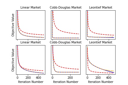
Figure 1: The first row describes the average trajectory of the value of the objective function for a randomly initialized market on each iteration of both Algorithm 3 (in blue) and Algorithm 4 (in orange) when the starting prices are high, while the second row describes the average trajectory of the objective function when starting prices are low for linear, Cobb-Douglas, and Leontief Fisher markets respectively. The dashed red line represents a convergence rate of $O(\nicefrac{{1}}{{\sqrt{T}}})$, which corresponds to an iteration complexity of $O(\nicefrac{{1}}{{\epsilon^{2}}})$.

In order to investigate whether the outputs of Algorithm 1, which uses an exact max-oracle (i.e., 0-max-oracle) are more precise than those of Algorithm 2, we solved 500 randomly initialized markets with both algorithms. We then ran a James’ first-order test Algina et al. (1994); Hernandez et al. (2021) on the mean output of both algorithms to see if their difference was statistically significant. Our calculations produced $p$-values of $0.69$, $0$, and $1.06\times 10^{-18}$, for Fisher markets with linear, Cobb-Douglas, and Leontief utilities, respectively. At a significance level of $0.05$, these results are not statistically significant for linear utilities only. This result can be attributed to the fact that the value function is not differentiable in the linear case, which makes the nested gradient descent/ascent algorithm less precise.

6 Conclusion

In this paper, we study a class of constrained convex-concave min-max optimization problems with dependent constraint sets, which we call convex-concave min-max Stackelberg games. As such games do not afford a minimax theorem in general, we focused on existence and computation of their Stackelberg equilibria. We established the existence of Stackelberg equilibria in these games, assuming continuous objective functions and suitable convexity assumptions on the players’ action sets. We then introduced a novel subdifferential envelope theorem, which formed the core of two subgradient methods with polynomial-time iteration complexity that converge to Stackelberg equilibria. Finally, we applied our theory to the computation of competitive equilibria in Fisher markets. This application yielded a new variant of the classic tâtonnement process, where, in addition to the auctioneer iteratively adjusting prices, the buyers iteratively compute their demands. A further question of interest both for Fisher market dynamics and convex-concave min-max Stackelberg games more generally is whether gradient-descent-ascent (GDA) converges in the dependent action set setting as it does in the independent action setting Lin et al. (2020a). GDA dynamics for Fisher markets correspond to myopic best-response dynamics (see, for example, Monderer and Shapley (1996)). We would expect such a result to be of computational as well as economic interest.

Appendix A Pseudo-Games and Generalized Nash Equilibria

A two-player, zero-sum pseudo-game (or abstract economy Arrow and Debreu [1954]) $(X,Y,f,\bm{g})$ comprises two players, $\bm{x}$ and $\bm{y}$, with respective payoff functions $-f(\bm{x},\bm{y})$ and $f(\bm{x},\bm{y})$, and respective action spaces given by the correspondences ${\mathcal{X}}:Y\rightrightarrows X$ and ${\mathcal{Y}}:X\rightrightarrows Y$, i.e., set-valued mappings, each of which depends on the choice the other player takes: i.e., ${\mathcal{X}}(\bm{y})=\left\{\bm{x}\in X\mid\bm{g}(\bm{x},\bm{y})\geq\bm{0}\right\}$ and ${\mathcal{Y}}(\bm{x})=\left\{\bm{y}\in Y\mid\bm{g}(\bm{x},\bm{y})\geq\bm{0}\right\}$. A generalized Nash equilibrium (GNE), the canonical solution concept in pseudo-games, is an action profile $(\bm{x}^{*},\bm{y}^{*})\in X\times Y$ s.t. $\bm{g}(\bm{x}^{*},\bm{y}^{*})\geq 0$ s.t.

$$\max_{\bm{y}\in Y:\bm{g}(\bm{x}^{*},\bm{y})\geq 0}f(\bm{x}^{*},\bm{y})\leq f(\bm{x}^{*},\bm{y}^{*})\leq\min_{\bm{x}\in X:\bm{g}(\bm{x},\bm{y}^{*})\geq 0}f(\bm{x},\bm{y}^{*})\enspace.$$ (4)

That is, at a GNE, players choose best responses to the other players’ strategies from within the space of strategies defined by the other players’ choices.

It is difficult to imagine a situation in which the players choose some $\bm{x}$ and $\bm{y}$ simultaneously and then, for some reason, it happens that the constraints $\bm{g}(\bm{x},\bm{y})\geq\bm{0}$ are satisfied Ichiishi [1983]. For this reason, a pseudo-game is not technically a game. If the players move sequentially, however, and only the inner player’s feasible set is constrained by the outer player’s choice (but not vice versa), then the pseudo-game is indeed a game—a Stackelberg game, to be precise.

When $f$ is convex-concave, and $g_{k}$ is concave for all $k\in[d]$, a GNE is guaranteed to exist Arrow and Debreu [1954]. The existence of a GNE, however, does not imply that a minimax theorem holds, which in turn means that Stackelberg equilibria of a pseudo-game need not coincide with its GNE:

Example A.1.

Consider the constrained min-max optimization problem $\min_{x\in[-1,1]}\max_{y\in[-1,1]:x+y\leq 0}x^{2}+y+1$ with optimum $x^{*}=\nicefrac{{1}}{{2}},y^{*}=-\nicefrac{{1}}{{2}}$ and value $\nicefrac{{3}}{{4}}$, as in Example 1.1. Now, consider the same problem (i.e., the same objective function and constraints), with the order of the $\min$ and the $\max$ reversed: $\max_{y\in[-1,1]}\min_{x\in[-1,1]:x+y\leq 0}x^{2}+y+1$. The optimum is now $x^{**}=-1,y^{**}=1$ with value $3$. The min-max optimum $(x^{*},y^{*})$ is not a GNE, because $x^{*}=\nicefrac{{1}}{{2}}$ is not a best response to $y^{*}=-\nicefrac{{1}}{{2}}$ over the set $\{x\in[-1,1]\mid x+y^{*}\leq 0\}$, e.g., the $\bm{x}$-player can do better by playing $x\in[-1,\nicefrac{{1}}{{2}})$. However, the max-min optimum $(x^{**},y^{**})$ is a GNE, because $y^{**}=1$ is a best response to $x^{**}=-1$ over the set $\{y\in[-1,1]\}$. In fact, this game has a set of GNEs $(x^{\prime},y^{\prime})$ given by $x^{\prime}\in[-1,0]$, and $y^{\prime}=-x^{\prime}$, with values in the set $[1,3]$ .

Because a minimax theorem does not hold for pseudo-games, the solutions to min-max Stackelberg games (i.e., Stackelberg equilibria) do not necessarily coincide with the GNE of the associated pseudo-game. Interestingly, the min-max (resp. max-min) value of the pseudo-game lower (resp. upper) bounds the value of the pseudo-game at any GNE. In other words, the payoff of the $\bm{x}$ (resp. $\bm{y}$) player at a GNE is no lower (resp. higher) than their payoff at any Stackelberg equilibrium: i.e.,

$$\min_{\bm{x}\in X}\max_{\bm{y}\in Y:\bm{g}(\bm{x},\bm{y})\geq 0}f(\bm{x},\bm{y})\leq f(\bm{x}^{*},\bm{y}^{*})\leq\max_{\bm{y}\in Y}\min_{\bm{x}\in X:\bm{g}(\bm{x},\bm{y})\geq 0}f(\bm{x},\bm{y})$$ (5)

This can be observed by taking the minimum over all $\bm{x}^{*}\in X$ on the left hand side of Equation 4:

$$\min_{\bm{x}\in X}\max_{\bm{y}\in Y:\bm{g}(\bm{x},\bm{y})\geq 0}f(\bm{x},\bm{y})\leq\max_{\bm{y}\in Y:\bm{g}(\bm{x}^{*},\bm{y})\geq 0}f(\bm{x}^{*},\bm{y})\leq f(\bm{x}^{*},\bm{y}^{*})\enspace,$$ (6)

and the maximum over all $\bm{y}^{*}\in Y$ on the right hand side of Equation 4

$$f(\bm{x}^{*},\bm{y}^{*})\leq\min_{\bm{x}\in X:\bm{g}(\bm{x},\bm{y}^{*})\geq 0}f(\bm{x},\bm{y}^{*})\leq\max_{\bm{y}\in Y}\min_{\bm{x}\in X:\bm{g}(\bm{x},\bm{y})\geq 0}f(\bm{x},\bm{y})\enspace.$$ (7)

Appendix B Omitted Proofs Section 2

See 3.2

Proof of Theorem 3.2.

By Theorem 5.9 of Rockafellar and Wets [2009], the constraint correspondence $C(\bm{x})=\left\{\bm{y}\in Y\mid\bm{g}(\bm{x},\bm{y})\geq\bm{0}\right\}$ is continuous, i.e., upper and lower hemi-continuous (see for instance chapter 5 of Rockafellar and Wets [2009]). Hence, by the Maximum Theorem Berge [1997], the outer player’s value function $V(\bm{x})=\max_{\bm{y}\in Y:\bm{g}(\bm{x},\bm{y})\geq\bm{0}}f(\bm{x},\bm{y})=\max_{\bm{y}\in C(\bm{x})}f(\bm{x},\bm{y})$ is continuous, and the inner player’s solution correspondence $Y^{*}(\bm{x})=\operatorname*{arg\,max}_{\bm{y}\in Y:\bm{g}(\bm{x},\bm{y})\geq\bm{0}}f(\bm{x},\bm{y})$ is non-empty, for all $\bm{x}\in X$. Since $V$ is continuous and $X$ is compact and non-empty, by the extreme value theorem Protter et al. [2012], there exists a minimizer $\bm{x}^{*}\in X$ of $V$. Hence $(\bm{x}^{*},\bm{y}^{*}(\bm{x}^{*}))$, with $\bm{y}^{*}(\bm{x}^{*})\in Y^{*}(\bm{x}^{*})$, is a Stackelberg equilibrium of $(X,Y,f,\bm{g})$.

Let $(\bm{x}_{1},\bm{y}_{1})$ and $(\bm{x}_{2},\bm{y}_{2})$ be two Stackelberg equilibria whose values differ. WLOG, suppose $f(\bm{x}_{1},\bm{y}_{1})>f(\bm{x}_{2},\bm{y}_{2})$, so that $V(\bm{x}_{1})=f(\bm{x}_{1},\bm{y}_{1})>f(\bm{x}_{2},\bm{y}_{2})=V(\bm{x}_{2})$, where the first and last equality follow from the definition of Stackelberg equilibrium. But then $(\bm{x}_{1},\bm{y}_{1})$ cannot be a Stackelberg equilibrium, since $\bm{x}_{1}$ is not a minimizer of the outer player’s value function. Therefore, there cannot exist two Stackelberg equilibria whose values differ, i.e., the value of all Stackelberg equilibria is unique. ∎

Proposition B.1.

Consider a min-max Stackelberg game $(X,Y,f,\bm{g})$. Suppose that 1. (Slater’s condition) $\forall\bm{x}\in X,\exists\widehat{\bm{y}}\in Y$ s.t. $g_{k}(\bm{x},\widehat{\bm{y}})>0$, for all $k\in[d]$. 2. $\nabla_{\bm{x}}f,\nabla_{\bm{x}}g_{1},\ldots,\nabla_{\bm{x}}g_{d}$ are continuous; 3^′a. $f$ is continuous and convex-concave, 3^′b. the constraints $\bm{g}$ are of the form $g_{1}(\bm{x},y_{1}),g_{2}(\bm{x},y_{2}),\ldots,g_{d}(\bm{x},y_{d})$ are continuous in $(\bm{x},\bm{y})$, and concave in $\bm{y}$, for all $\bm{x}\in X$; 3^′c. for all $k\in[d]$, $\bm{x}\in X$, and $\bm{y}\in Y$, $\frac{-\nabla_{y_{k}}f(\bm{x},\bm{y})}{\nabla_{{y_{k}}}g_{k}(\bm{x},y_{k})}g_{k}(\bm{x},y_{k})$ is convex in $\bm{x}$. Then the value function $V$ associated with $(X,Y,f,\bm{g})$ is convex.

Proof of Proposition B.1.

By the Maximum Theorem Berge [1997], the outer player’s value function is continuous.

Define ${\mathcal{L}}:Y\times\mathbb{R}_{+}^{d}\times X\to\mathbb{R}$ s.t. ${\mathcal{L}}(\bm{y},\bm{\lambda};\bm{x})=f(\bm{x},\bm{y})+\sum_{k=1}^{d}\lambda_{k}g_{k}(\bm{x},\bm{y})$ . Since Slater’s condition is satisfied, the KKT theorem Kuhn and Tucker [1951] applies, which means that for all $\bm{x}\in X$ and $\bm{y}\in Y$, the optimal KKT multipliers $\bm{\lambda}^{*}$ exist, and thus:

$$\nabla_{\bm{y}}f(\bm{x},\bm{y})+\sum_{k=1}^{d}\lambda_{k}^{*}\nabla_{\bm{y}}g_{k}(\bm{x},\bm{y})=\bm{0}$$ (8)

$$\nabla_{\bm{y}}f(\bm{x},\bm{y})+\sum_{k=1}^{d}\lambda_{k}^{*}\nabla_{\bm{y}}g_{k}(\bm{x},y_{k})=\bm{0}$$ (Assumption 3^′b) (9)

$$\nabla_{y_{k}}f(\bm{x},\bm{y})+\sum_{k=1}^{d}\lambda_{k}^{*}\nabla_{y_{k}}g_{k}(\bm{x},y_{k})=\bm{0}$$ (10)

$$\lambda_{k}^{*}=\frac{-\nabla_{y_{k}}f(\bm{x},\bm{y})}{\nabla_{y_{k}}g_{k}(\bm{x},y_{k})} \forall k\in[d]$$ (11)

Plugging the optimal KKT multipliers back into the Lagrangian, we obtain:

$$V(\bm{x})=\max_{\bm{y}\in Y}{\mathcal{L}}(\bm{y},\bm{\lambda}^{*}(\bm{x},\bm{y});\bm{x})=\max_{\bm{y}\in Y}f(\bm{x},\bm{y})+\sum_{k=1}^{d}\frac{-\nabla_{y_{k}}f(\bm{x},\bm{y})}{\nabla_{y_{k}}g_{k}(\bm{x},y_{k})}g_{k}(\bm{x},y_{k})$$ (12)

By Assumption 3^′c, for all $k\in[d]$, $\frac{-\nabla_{y_{k}}f(\bm{x},\bm{y})}{\nabla_{y_{k}}g_{k}(\bm{x},y_{k})}g_{k}(\bm{x},y_{k})$, and by Assumption 3^′a, $f(\bm{x},\bm{y})$ are convex in $\bm{x}$, for all $\bm{y}\in Y$. Therefore, $f(\bm{x},\bm{y})+\sum_{k=1}^{d}\frac{-\nabla_{y_{k}}f(\bm{x},\bm{y})}{\nabla_{y_{k}}g_{k}(\bm{x},y_{k})}g_{k}(\bm{x},y_{k})$ is convex in $\bm{x}\in X$, for all $\bm{y}\in Y$. Finally, by Danskin’s theorem, $V(\bm{x})=\max_{\bm{y}\in Y}f(\bm{x},\bm{y})+\sum_{k=1}^{d}\frac{-\nabla_{y_{k}}f(\bm{x},\bm{y})}{\nabla_{y_{k}}g_{k}(\bm{x},y_{k})}g_{k}(\bm{x},y_{k})$ is convex as well.

∎

See 3.4

Proof of Proposition 3.4.

By Theorem 3.2, the set of Stackelberg equilibria of any min-max Stackelberg game is non-empty. Additionally, under 3.3, we have that for all $\bm{x}\in{\mathcal{X}}$, $f(\bm{x},\cdot)$ is concave, and $\{\bm{y}\in Y\mid\bm{g}(\bm{x},\bm{y})\geq\bm{0}\}$ is convex. Hence, by Theorem 2.6 of Rockafeller Rockafellar and Wets [2009], the set of solutions $Y^{*}(\bm{x})=\operatorname*{arg\,max}_{\bm{y}\in Y:\bm{g}(\bm{x},\bm{y})\geq\bm{0}}f(\bm{x},\bm{y})$ is compact- and convex- valued. Similarly, by Proposition B.1, under 3.1, $\max_{\bm{y}\in Y:\bm{g}(\bm{x},\bm{y})\geq\bm{0}}f(\bm{x},\bm{y})$ is continuous and convex. Hence, the set of solutions $X^{*}=\operatorname*{arg\,min}_{\bm{x}\in X}\max_{\bm{y}\in Y:\bm{g}(\bm{x},\bm{y})\geq\bm{0}}f(\bm{x},\bm{y})$ is compact- and convex-valued. Since the composition of two compact-convex-valued correspondences is again compact-convex-valued (Proposition 5.52 of Rockafeller Rockafellar and Wets [2009]), we conclude that the set of Stackelberg equilibria, namely $X^{*}(Y^{*})$, is compact and convex. ∎

Appendix C Envelope Theorem

Danskin’s theorem Danskin [1966] offers insights into optimization problems of the form: $\max_{\bm{y}\in Y}f(\bm{x},\bm{y})$, where $Y\subset\mathbb{R}^{m}$ is compact and non-empty. Among other things, Danskin’s theorem allows us to compute the gradient of the objective function of this optimization problem with respect to $\bm{x}$.

Theorem C.1 (Danskin’s Theorem).

Consider an optimization problem of the form: $\max_{\bm{y}\in Y}f(\bm{x},\bm{y})$, where $Y\subset\mathbb{R}^{m}$ is compact and non-empty. Suppose that $Y$ is convex and that $f$ is concave in $\bm{y}$. Let $V(\bm{x})=\max_{\bm{y}\in Y}f(\bm{x},\bm{y})$ and $Y^{*}(\bm{x})=\operatorname*{arg\,max}_{\bm{y}\in Y}f(\bm{x},\bm{y})$. Then $V$ is differentiable at $\widehat{\bm{x}}$, if the solution correspondence $Y^{*}(\widehat{\bm{x}})$ is a singleton: i.e., $Y^{*}(\widehat{\bm{x}})=\{\bm{y}^{*}(\widehat{\bm{x}})\}$. Additionally, the gradient at $\widehat{\bm{x}}$ is given by $V^{\prime}(\widehat{\bm{x}})=\nabla_{\bm{x}}f(\widehat{\bm{x}},\bm{y}^{*}(\widehat{\bm{x}}))$.

Unfortunately, Danskin’s theorem does not hold when the set $Y$ is replaced by a correspondence, which occurs in min-max Stackelberg games: i.e., when the inner problem is $\max_{\bm{y}\in Y:\bm{g}(\bm{x},\bm{y})\geq\bm{0}}f(\bm{x},\bm{y})$.

Example C.2 (Danskin’s theorem does not apply to min-max Stackelberg games).

Consider the optimization problem:

$$\max_{y\in\mathbb{R}:y+x\geq 0}-y^{2}+y+2x+2\enspace.$$ (13)

The solution to this problem is unique, given any $x\in X$, meaning the solution correspondence $Y^{*}(x)$ is singleton-valued. We denote this unique solution by $y^{*}(x)$. After solving, we find that

$$y^{*}(x)=\left\{\begin{array}[]{cc}\nicefrac{{1}}{{2}}&\text{ if }x\geq-\nicefrac{{1}}{{2}}\\ -x&\text{ if }x<-\nicefrac{{1}}{{2}}\end{array}\right.$$ (16)

The value function $V(x)=\max_{y\in\mathbb{R}:y+x\geq 0}-y^{2}+y+2x+2$ is then given by:

$$V(x) =f(x,y^{*}(x))$$ (17)

$$=-y^{*}(x)^{2}+y^{*}(x)+2x+2$$ (18)

$$=\left\{\begin{array}[]{cc}-\nicefrac{{1}}{{4}}+\nicefrac{{1}}{{2}}+2x+2&\text{ if }x\geq-\nicefrac{{1}}{{2}}\\ -x^{2}-x+2x+2&\text{ if }x<-\nicefrac{{1}}{{2}}\end{array}\right.$$ (21)

$$=\left\{\begin{array}[]{cc}\nicefrac{{9}}{{4}}+2x&\text{ if }x\geq-\nicefrac{{1}}{{2}}\\ -x^{2}+x+2&\text{ if }x<-\nicefrac{{1}}{{2}}\end{array}\right.$$ (24)

The derivative of this value function is:

$$\frac{\partial V}{\partial x} =\left\{\begin{array}[]{cc}2&\text{ if }x\geq-\nicefrac{{1}}{{2}}\\ 1-2x&\text{ if }x<-\nicefrac{{1}}{{2}}\end{array}\right.$$ (27)

However, the derivative predicted by Danskin’s theorem is 2. Hence, Danskin’s theorem does not hold when the constraints are parameterized, i.e., when the problem is of the form $\min_{\bm{y}\in Y:\bm{g}(\bm{x},\bm{y})}f(\bm{x},\bm{y})$ rather than $\min_{\bm{y}\in Y}f(\bm{x},\bm{y})$, where $X\subset\mathbb{R}^{n}$, $Y\subset\mathbb{R}^{m}$, and for all $k\in[d]$, $g_{k}:X\times Y\to\mathbb{R}$ are continuous.

N.B. For simplicity, we do not assume the constraint set is compact in this example. Compactness of the constraint set can be used to guarantee existence of a solution, but as a solution to this particular problem always exists, we can do away with this assumption.

The following theorem, due to Milgrom and Segal [2002], generalizes Danskin’s theorem to handle parameterized constraints:

Theorem C.3 (Envelope Theorem Milgrom and Segal [2002]).

Consider the maximization problem

$$V(\bm{x})=\max_{\bm{y}\in Y}f(\bm{x},\bm{y}),\text{ subject to }g_{k}(\bm{x},\bm{y})\geq 0,\text{ for all }k=1,\ldots,d\enspace,$$ (28)

where $Y\subseteq\mathbb{R}^{m}$.

Define the solution correspondence $Y^{*}(\bm{x})=\operatorname*{arg\,max}_{\bm{y}\in X:\bm{g}(\bm{x},\bm{y})\geq\bm{0}}f(\bm{x},\bm{y})$. If 3.3 holds, then the value function $V$ is absolutely continuous, and at any point $\widehat{\bm{x}}\in X$ where $V$ is differentiable:

$$\nabla_{\bm{x}}V(\widehat{\bm{x}})=\nabla_{\bm{x}}L(\bm{y}^{*}(\widehat{\bm{x}}),\bm{\lambda}^{*}(\widehat{\bm{x}},\bm{y}^{*}(\widehat{\bm{x}}))),\widehat{\bm{x}})=\nabla_{\bm{x}}f\left(\widehat{\bm{x}},\bm{y}^{*}(\widehat{\bm{x}})\right)+\sum_{k=1}^{d}\lambda_{k}^{*}(\widehat{\bm{x}},\bm{y}^{*}(\widehat{\bm{x}}))\nabla_{\bm{x}}g_{k}\left(\widehat{\bm{x}},\bm{y}^{*}(\widehat{\bm{x}})\right)\enspace,$$ (29)

where $\bm{\lambda}^{*}(\widehat{\bm{x}},\bm{y}^{*}(\widehat{\bm{x}}))=\left(\lambda_{1}(\widehat{\bm{x}},\bm{y}^{*}(\widehat{\bm{x}})),\ldots,\lambda_{d}^{*}(\widehat{\bm{x}},\bm{y}^{*}(\widehat{\bm{x}}))\right)^{T}\in\Lambda^{*}(\widehat{\bm{x}},\bm{y}^{*}(\widehat{\bm{x}}))$ are the KKT multipliers associated associated with $\bm{y}^{*}(\widehat{\bm{x}})\in Y^{*}(\widehat{\bm{x}})$.

Appendix D Omitted Subdifferential Envelope Theorem Proof (Section 4)

Proof of Theorem 4.1.

As usual, let $V(\bm{x})=\max_{\bm{y}\in Y:\bm{g}(\bm{x},\bm{y})\geq 0}f(\bm{x},\bm{y})$. First, note that Proposition B.1 $V$ is subdifferentiable as it is convex Boyd and Vandenberghe [2018]. Reformulating the problem as a Lagrangian saddle point problem, for all $\widehat{\bm{x}}\in X$, it holds that:

$$V(\widehat{\bm{x}}) =\max_{\bm{y}\in Y:\bm{g}(\widehat{\bm{x}},\bm{y})\geq 0}f(\widehat{\bm{x}},\bm{y})$$ (30)

$$=\max_{\bm{y}\in Y}\min_{\bm{\lambda}\in\mathbb{R}^{d}_{++}}\left\{f(\widehat{\bm{x}},\bm{y})+\sum_{k=1}^{d}\lambda_{k}g_{k}(\widehat{\bm{x}},\bm{y})\right\}$$ (31)

Since $f$ is continuous, $Y$ is compact, and $g_{1},\ldots,g_{d}$ are continuous, for all $\widehat{\bm{x}}\in X$, there exists $\bm{y}^{*}(\widehat{\bm{x}})\in\operatorname*{arg\,max}_{\bm{y}\in Y:\bm{g}(\widehat{\bm{x}},\bm{y})\geq\bm{0}}f(\widehat{\bm{x}},\bm{y})$. Furthermore, as 3.3 ensures that an interior solution exists, the Karush-Kuhn-Tucker Theorem Kuhn and Tucker [1951] applies, so for all $\widehat{\bm{x}}\in X$ and any associated $\bm{y}^{*}(\widehat{\bm{x}})$, there exists $\bm{\lambda}(\widehat{\bm{x}},\bm{y}^{*}(\widehat{\bm{x}}))\in\mathbb{R}^{d}$ that solves Equation 31.

Define the solution correspondence $Y^{*}(\bm{x})=\operatorname*{arg\,max}_{\bm{y}\in Y:\bm{g}(\bm{x},\bm{y})\geq 0}f(\bm{x},\bm{y})$, and let $\Lambda^{*}(\bm{x},\bm{y})=\operatorname*{arg\,min}_{\bm{\lambda}\in\mathbb{R}^{d}_{+}}\left\{f(\bm{x},\bm{y})+\sum_{k=1}^{d}\lambda_{k}g_{k}(\bm{x},\bm{y})\right\}$. We can then re-express the value function at $\widehat{\bm{x}}$ as:

$$V(\widehat{\bm{x}})=f(\widehat{\bm{x}},\bm{y}^{*}(\widehat{\bm{x}}))+\sum_{k=1}^{d}\lambda_{k}^{*}(\widehat{\bm{x}},\bm{y}^{*}(\widehat{\bm{x}}))g_{k}(\widehat{\bm{x}},\bm{y}^{*}(\widehat{\bm{x}})), \forall\bm{y}^{*}(\widehat{\bm{x}})\in Y^{*}(\widehat{\bm{x}}),\lambda_{k}^{*}(\widehat{\bm{x}},\bm{y}^{*}(\widehat{\bm{x}}))\in\Lambda^{*}(\widehat{\bm{x}},\bm{y}^{*}(\widehat{\bm{x}}))\enspace.$$

Equivalently, we can take the maximum over $\bm{y}^{*}$’s and $\bm{\lambda}^{*}$’s to obtain:

$$V(\widehat{\bm{x}}) =\max_{\bm{y}^{*}(\widehat{\bm{x}})\in Y^{*}(\widehat{\bm{x}})}\max_{\lambda_{k}^{*}(\widehat{\bm{x}},\bm{y}^{*}(\widehat{\bm{x}}))\in\Lambda^{*}(\widehat{\bm{x}},\bm{y}^{*}(\widehat{\bm{x}}))}\left\{f(\widehat{\bm{x}},\bm{y})+\sum_{k=1}^{d}\lambda_{k}^{*}(\widehat{\bm{x}},\bm{y}^{*}(\widehat{\bm{x}}))g_{k}(\widehat{\bm{x}},\bm{y})\right\}\enspace.$$

Note that for fixed $\bm{y}^{*}(\widehat{\bm{x}})\in Y^{*}(\widehat{\bm{x}})$ and corresponding fixed $\lambda_{k}^{*}(\widehat{\bm{x}},\bm{y}^{*}(\widehat{\bm{x}}))\in\Lambda^{*}(\widehat{\bm{x}},\bm{y}^{*}(\widehat{\bm{x}}))$,
$f(\widehat{\bm{x}},\bm{y})+\sum_{k=1}^{d}\lambda_{k}^{*}(\widehat{\bm{x}},\bm{y}^{*}(\widehat{\bm{x}}))g_{k}(\widehat{\bm{x}},\bm{y}^{*}(\widehat{\bm{x}}))$ is differentiable, since $f,g_{1},\ldots,g_{d}$ are differentiable.

Additionally, recall the pointwise maximum subdifferential property, i.e., if $f(\bm{x})=\max_{\alpha\in{\mathcal{A}}}f_{\alpha}(\bm{x})$ for a family of functions $\{f_{\alpha}\}_{\alpha\in{\mathcal{A}}}$, then $\partial_{\bm{x}}f({\bm{a}})=\mathrm{conv}\left(\bigcup_{\alpha\in{\mathcal{A}}}\left\{\partial_{\bm{x}}f_{\alpha\in{\mathcal{A}}}({\bm{a}})\mid f_{\alpha}({\bm{a}})=f(\bm{x})\right\}\right)$, which then gives:

$$\partial_{\bm{x}}V(\widehat{\bm{x}}) =\partial_{\bm{x}}\left(\max_{\bm{y}^{*}(\widehat{\bm{x}})\in Y^{*}(\widehat{\bm{x}})}\max_{\lambda_{k}^{*}(\widehat{\bm{x}},\bm{y}^{*}(\widehat{\bm{x}}))\in\Lambda^{*}(\widehat{\bm{x}},\bm{y}^{*}(\widehat{\bm{x}}))}\left\{f(\widehat{\bm{x}},\bm{y}^{*}(\widehat{\bm{x}}))+\sum_{k=1}^{d}\lambda_{k}^{*}(\widehat{\bm{x}},\bm{y}^{*}(\widehat{\bm{x}}))g_{k}(\widehat{\bm{x}},\bm{y}^{*}(\widehat{\bm{x}}))\right\}\right)$$ (32)

$$=\mathrm{conv}\left(\bigcup_{\bm{y}^{*}(\widehat{\bm{x}})\in Y^{*}(\widehat{\bm{x}})}\bigcup_{\lambda_{k}^{*}(\widehat{\bm{x}},\bm{y}^{*}(\widehat{\bm{x}}))\in\Lambda^{*}(\widehat{\bm{x}},\bm{y}^{*}(\widehat{\bm{x}}))}\partial_{\bm{x}}\left\{f(\widehat{\bm{x}},\bm{y}^{*}(\widehat{\bm{x}}))+\sum_{k=1}^{d}\lambda_{k}^{*}(\widehat{\bm{x}},\bm{y}^{*}(\widehat{\bm{x}}))g_{k}(\widehat{\bm{x}},\bm{y}^{*}(\widehat{\bm{x}}))\right\}\right)$$ (33)

$$=\mathrm{conv}\left(\bigcup_{\bm{y}^{*}(\widehat{\bm{x}})\in Y^{*}(\widehat{\bm{x}})}\bigcup_{\lambda_{k}^{*}(\widehat{\bm{x}},\bm{y}^{*}(\widehat{\bm{x}}))\in\Lambda^{*}(\widehat{\bm{x}},\bm{y}^{*}(\widehat{\bm{x}}))}\left\{\nabla_{\bm{x}}f\left(\widehat{\bm{x}},\bm{y}^{*}(\widehat{\bm{x}})\right)+\sum_{k=1}^{d}\lambda_{k}^{*}(\widehat{\bm{x}},\bm{y}^{*}(\widehat{\bm{x}}))\nabla_{\bm{x}}g_{k}\left(\widehat{\bm{x}},\bm{y}^{*}(\widehat{\bm{x}})\right)\right\}\right)\enspace.$$ (34)

∎

Appendix E Convergence Results for Section 4

Proof of Theorem 4.2.

By our subdifferential envelope theorem (Theorem 4.1), we have:

$$\nabla_{\bm{x}}f(\bm{x}^{(t-1)},\bm{y}^{(t-1)})+\sum_{k=1}^{d}\lambda_{k}^{(t-1)}\nabla_{\bm{x}}g_{k}(\bm{x}^{(t-1)},\bm{y}^{(t-1)}) \in\partial_{\bm{x}}V(\bm{x}^{(t-1)})$$ (35)

$$=\partial_{\bm{x}}\max_{\bm{y}\in Y:\bm{g}(\bm{x}^{(t-1)},\bm{y})\geq 0}f(\bm{x}^{(t-1)},\bm{y})\enspace.$$ (36)

For notational clarity, let $\bm{h}(t-1)=\nabla_{\bm{x}}f(\bm{x}^{(t-1)},\bm{y}^{(t-1)})+\sum_{k=1}^{d}\lambda_{k}^{(t-1)}\nabla_{\bm{x}}g_{k}(\bm{x}^{(t-1)},\bm{y}^{(t-1)})$. Suppose that $\bm{x}^{*}\in\operatorname*{arg\,min}_{\bm{x}\in X}\max_{\bm{y}\in Y:\bm{g}(\bm{x},\bm{y})\geq\bm{0}}f(\bm{x},\bm{y})$. Then:

$$\left\|\bm{x}^{(T)}-\bm{x}^{*}\right\|^{2}$$ (37)

$$=\left\|\Pi_{X}\left(\bm{x}^{(T-1)}-\eta_{T}\bm{h}(T-1)\right)-\Pi_{X}\left(\bm{x}^{*}\right)\right\|^{2}$$ (38)

$$\leq\left\|\bm{x}^{(T-1)}-\eta_{T}\bm{h}(T-1)-\bm{x}^{*}\right\|^{2}$$ (39)

$$=\left\|\bm{x}^{(T-1)}-\bm{x}^{*}\right\|^{2}-2\eta_{T}\left<\bm{h}(T-1),\left(\bm{x}^{(T-1)}-\bm{x}^{*}\right)\right>+\eta_{T}^{2}\left\|\bm{h}(T-1)\right\|^{2}\enspace,$$ (40)

where the first line follows from the subgradient descent rule and the fact that $\bm{x}^{*}\in X$; the second, because the project operator is a non-expansion; and the third, by the definition of the norm.

Let for any $t\in\mathbb{N}_{+}$, $\mathrm{err}^{(t)}=\left<\bm{h}(t)-\nabla V(\bm{x}^{(t)}),\left(\bm{x}^{(t)}-\bm{x}^{*}\right)\right>$:

$$=\left\|\bm{x}^{(t-1)}-\bm{x}^{*}\right\|^{2}-2\eta_{t}\left<\nabla V(\bm{x}^{(t-1)}),\left(\bm{x}^{(t-1)}-\bm{x}^{*}\right)\right>-2\eta_{t}\left<\bm{h}(t-1)-\nabla V(\bm{x}^{(t-1)}),\left(\bm{x}^{(t-1)}-\bm{x}^{*}\right)\right>$$

$$+\eta_{t}^{2}\left\|\bm{h}(t-1)\right\|^{2}$$ (41)

$$=\left\|\bm{x}^{(t-1)}-\bm{x}^{*}\right\|^{2}-2\eta_{t}\left<\nabla V(\bm{x}^{(t-1)}),\left(\bm{x}^{(t-1)}-\bm{x}^{*}\right)\right>-2\eta_{t}\mathrm{err}^{(t-1)}+\eta_{t}^{2}\left\|\bm{h}(t-1)\right\|^{2}$$ (42)

$$\leq\left\|\bm{x}^{(t-1)}-\bm{x}^{*}\right\|^{2}-2\eta_{t}\left(V(\bm{x}^{(t-1)})-V(\bm{x}^{*})\right)-2\eta_{t}\mathrm{err}^{(t-1)}+\eta_{t}^{2}\left\|\bm{h}(t-1)\right\|^{2}\enspace,$$ (43)

where the last line follows by the definition of the subgradient, i.e., $\left<\nabla V(\bm{x}^{(t-1)}),\left(\bm{x}^{(t-1)}-\bm{x}^{*}\right)\right>\geq f(\bm{x}^{(t-1)},\bm{y}^{(t-1)})-f(\bm{x}^{*},\bm{y}^{(t-1)})$. Applying this inequality recursively, we obtain:

$$\left\|\bm{x}^{(t)}-\bm{x}^{*}\right\|^{2}\leq\left\|\bm{x}^{(0)}-\bm{x}^{*}\right\|^{2}-\sum_{t=1}^{t}2\eta_{t}\left(V(\bm{x}^{(t-1)})-V(\bm{x}^{*})\right)-\sum_{t=1}^{t}2\eta_{t}\mathrm{err}^{(t-1)}+\sum_{t=1}^{t}\eta_{t}^{2}\left\|\bm{h}(t-1)\right\|^{2}\enspace.$$ (44)

Since $\left\|\bm{x}^{(t)}-\bm{x}^{*}\right\|\geq 0$, re-organizing, we have:

$$2\sum_{t=1}^{T}\eta_{t}\left(V(\bm{x}^{(T-1)})-V(\bm{x}^{*})\right)\leq\left\|\bm{x}^{(0)}-\bm{x}^{*}\right\|^{2}-\sum_{t=1}^{T}2\eta_{T}\mathrm{err}^{(T-1)}+\sum_{t=1}^{T}\eta_{t}^{2}\left\|\bm{h}(t-1)\right\|^{2}\enspace.$$ (45)

Let $(\bm{x}^{(t)}_{\mathrm{best}},\bm{y}^{(t)}_{\mathrm{best}})=(\bm{x}^{(k^{*})},\bm{y}^{(k^{*})})$ where $k^{*}\in\operatorname*{arg\,min}_{k\in[t]}V(\bm{x}^{(k)})$. Then:

$$\sum_{t=1}^{T}\eta_{t}\left(V(\bm{x}^{(T-1)})-V(\bm{x}^{*})\right)$$ (46)

$$\geq\left(\sum_{t=1}^{T}\eta_{t}\right)\min_{t\in[T]}\left(V(\bm{x}^{(T-1)})-V(\bm{x}^{*})\right)$$ (47)

$$=\left(\sum_{t=1}^{T}\eta_{t}\right)\left(V(\bm{x}^{(T-1)}_{\mathrm{best}})-V(\bm{x}^{*})\right)$$ (48)

Combining the above inequality with Equation 44, we get the following bound:

$$V(\bm{x}^{(T-1)}_{\mathrm{best}})-V(\bm{x}^{*})\leq\frac{\left\|\bm{x}^{(0)}-\bm{x}^{*}\right\|^{2}-\sum_{t=1}^{T}2\eta_{t}\mathrm{err}^{(t-1)}+\sum_{t=1}^{T}\eta_{t}^{2}||\bm{h}(t-1)||^{2}}{2\left(\sum_{t=1}^{T}\eta_{t}\right)}$$ (49)

Now, since the value function $V$ is $\ell_{V}$-Lipschitz continuous, where $\ell_{V}=\max_{(\widehat{\bm{x}},\widehat{\bm{y}})\in X\times Y}\left\|\nabla_{\bm{x}}f\left(\widehat{\bm{x}},\bm{y}^{*}(\widehat{\bm{x}})\right)+\sum_{k=1}^{d}\lambda_{k}^{*}(\widehat{\bm{x}},\bm{y}^{*}(\widehat{\bm{x}}))\nabla_{\bm{x}}g_{k}\left(\widehat{\bm{x}},\bm{y}^{*}(\widehat{\bm{x}})\right)\right\|$ and $\bm{\lambda}^{*}(\widehat{\bm{x}},\bm{y}^{*}(\widehat{\bm{x}}))$ are the optimal KKT multipliers associated with $\bm{y}^{*}(\widehat{\bm{x}})\in\operatorname*{arg\,max}_{\bm{y}\in Y:\bm{g}(\widehat{\bm{x}},\bm{y})\geq\bm{0}}f(\bm{x},\bm{y})$, all the subgradients are bounded: i.e., for all $k\in\mathbb{N},\left\|\bm{h}(k-1)\right\|\leq\ell_{V}$. So:

$$V(\bm{x}^{(T-1)}_{\mathrm{best}})-V(\bm{x}^{*}) \leq\frac{\left\|\bm{x}^{(0)}-\bm{x}^{*}\right\|^{2}-\sum_{t=1}^{T}2\eta_{t}\mathrm{err}^{(t-1)}+\ell_{V}^{2}\sum_{t=1}^{T}\eta_{t}^{2}}{2\left(\sum_{t=1}^{T}\eta_{t}\right)}$$ (50)

$$\frac{\left\|\bm{x}^{(0)}-\bm{x}^{*}\right\|^{2}+\sum_{t=1}^{T}2\eta_{t}\left|\mathrm{err}^{(t-1)}\right|+\ell_{V}^{2}\sum_{t=1}^{T}\eta_{t}^{2}}{2\left(\sum_{t=1}^{T}\eta_{t}\right)}$$ (51)

Letting $\overline{\mathrm{err}^{(T)}}\doteq\frac{\sum_{t=1}^{T}\eta_{t}\left|\mathrm{err}^{(t-1)}\right|}{\sum_{t=1}^{T}\eta_{t}}$, we get:

$$f(\bm{x}^{(T)}_{\mathrm{best}},\bm{x}^{(T)}_{\mathrm{best}})-\min_{\bm{x}\in X}\max_{\bm{y}\in Y:\bm{g}(\bm{x},\bm{y})\geq 0}f(\bm{x},\bm{y}) \leq\frac{\left\|\bm{x}^{(0)}-\bm{x}^{*}\right\|^{2}+\ell_{V}\sum_{t=1}^{T}\eta_{t}^{2}}{2\left(\sum_{t=1}^{T}\eta_{t}\right)}+\overline{\mathrm{err}^{(T)}}$$ (52)

Recall the assumptions that the step sizes are square-summable but not summable, namely $\sum_{k=1}^{T}\eta_{k}^{2}\leq\infty$ and $\sum_{k=1}^{T}\eta_{k}=\infty$. Now as $T\to\infty$, Equation 52 becomes:

$$\lim_{k\to\infty}f(\bm{x}^{(k)}_{\mathrm{best}},\bm{y}^{(k)}_{\mathrm{best}})\leq\min_{\bm{x}\in X}\max_{\bm{y}\in Y:\bm{g}(\bm{x},\bm{y})\geq 0}f(\bm{x},\bm{y})+\overline{\mathrm{err}^{(T)}}\enspace.$$ (53)

We have thus proven the first inequality of the two that define an $(\overline{\mathrm{err}^{(T)}},\delta)$-Stackelberg equilibrium.

The second inequality follows by construction, as for all $k\in\mathbb{N}$, the max oracle returns $\bm{y}^{(k)}_{\mathrm{best}}$ that satisfies $f(\bm{x}^{(k)}_{\mathrm{best}},\bm{y}^{(k)}_{\mathrm{best}})\geq\max_{\bm{y}\in Y:\bm{g}(\bm{x},\bm{y})\geq 0}f(\bm{x}^{(k)}_{\mathrm{best}},\bm{y})-\delta$. Thus, as $k\to\infty$, the best iterate converges to an $(\overline{\mathrm{err}^{(T)}},\delta)$-Stackelberg equilibrium. Additionally, setting $\eta_{t}=\frac{\left\|\bm{x}^{(0)}-\bm{x}^{*}\right\|}{\sqrt{T}}$, we see that for all $t\in[T]$,

$$f(\bm{x}^{(T)}_{\mathrm{best}},\bm{x}^{(T)}_{\mathrm{best}})-\min_{\bm{x}\in X}\max_{\bm{y}\in Y:\bm{g}(\bm{x},\bm{y})\geq 0}f(\bm{x},\bm{y}) \leq\frac{\left\|\bm{x}^{(0)}-\bm{x}^{*}\right\|^{2}}{\sqrt{T}}+\overline{\mathrm{err}^{(T)}}\enspace.$$ (54)

Likewise, setting $\varepsilon\leq\frac{\left\|\bm{x}^{(0)}-\bm{x}^{*}\right\|^{2}}{\sqrt{T}}$, we obtain $T\leq\frac{\left\|\bm{x}^{(0)}-\bm{x}^{*}\right\|^{4}}{\varepsilon^{2}}$, implying that the best iterate converges to an $(\varepsilon+\overline{\mathrm{err}^{(T)}},\delta)$-Stackelberg equilibrium in $O(\varepsilon^{-2})$ iterations.

Finally, by the Cauchy-Schwarz inequality, $|\mathrm{err}^{(T-1)}|\leq\left\|\bm{h}(t)-\nabla V(\bm{x}^{(t)})\right\|\left\|\bm{x}^{(t)}-\bm{x}^{*}\right\|$, giving us the theorem statement.

∎

Theorem E.1.

Suppose Algorithm 1 is run on min-max Stackelberg game given by $(X,Y,f,\bm{g})$ which satisfies 3.3, and that $V$ is $\mu$-strongly convex in $\bm{x}$. Then, if $(\bm{x}^{(t)}_{\mathrm{best}},\bm{y}^{(t)}_{\mathrm{best}})\in\operatorname*{arg\,min}_{(\bm{x}^{(k)},\bm{y}^{(k)}):k\in[t]}f(\bm{x}^{(k)},\bm{y}^{(k)})$, for $\varepsilon\in(0,1)$, and for all $t\in T$ $\eta_{t}=\frac{2}{\mu(t+1)}$, if we choose $T\geq N_{T}(\varepsilon)\in O(\varepsilon^{-1})$, then there exists an iteration $T^{*}\leq T$ s.t. $(\bm{x}^{(T^{*})}_{\mathrm{best}},\bm{y}^{(T^{*})}_{\mathrm{best}})$ is an $(\frac{8\ell_{V}(c)}{\mu},\delta)$-Stackelberg equilibrium.

Proof of Theorem E.1.

For notational clarity, let $\bm{h}(t-1)=\nabla_{\bm{x}}f(\bm{x}^{(t-1)},\bm{y}^{(t-1)})+\sum_{k=1}^{d}\lambda_{k}^{(t-1)}\nabla_{\bm{x}}g_{k}(\bm{x}^{(t-1)},\bm{y}^{(t-1)})$. Suppose that $\bm{x}^{*}\in\operatorname*{arg\,min}_{\bm{x}\in X}\max_{\bm{y}\in Y:\bm{g}(\bm{x},\bm{y})}f(\bm{x},\bm{y})$. Then, for all $t\in\mathbb{N}$ s.t. $t\geq 1$, we have:

$$\left\|\bm{x}^{(t)}-\bm{x}^{*}\right\|^{2}$$ (55)

$$=\left\|\Pi_{X}\left(\bm{x}^{(t-1)}-\eta_{t}\bm{h}(t-1)\right)-\Pi_{X}\left(\bm{x}^{*}\right)\right\|^{2}$$ (56)

$$\leq\left\|\bm{x}^{(t-1)}-\eta_{t}\bm{h}(t-1)-\bm{x}^{*}\right\|^{2}$$ (57)

$$=\left\|\bm{x}^{(t-1)}-\bm{x}^{*}\right\|^{2}-2\eta_{t}\left<\bm{h}(t-1),\left(\bm{x}^{(t-1)}-\bm{x}^{*}\right)\right>+\eta_{t}^{2}\left\|\bm{h}(t-1)\right\|^{2}$$ (58)

where the first line follows from the subgradient method’s update rule and the fact that $\bm{x}^{*}\in X$; the second, because the project operator is a non-expansion; and the third, by the definition of the norm.

Let for any $t\in\mathbb{N}_{+}$, $\mathrm{err}^{(t)}=\left<\bm{h}(t)-\nabla V(\bm{x}^{(t)}),\left(\bm{x}^{(t)}-\bm{x}^{*}\right)\right>$:

$$=\left\|\bm{x}^{(t-1)}-\bm{x}^{*}\right\|^{2}-2\eta_{t}\left<\nabla V(\bm{x}^{(t-1)}),\left(\bm{x}^{(t-1)}-\bm{x}^{*}\right)\right>-2\eta_{t}\left<\bm{h}(t-1)-\nabla V(\bm{x}^{(t-1)}),\left(\bm{x}^{(t-1)}-\bm{x}^{*}\right)\right>$$

$$+\eta_{t}^{2}\left\|\bm{h}(t-1)\right\|^{2}$$ (59)

$$=\left\|\bm{x}^{(t-1)}-\bm{x}^{*}\right\|^{2}-2\eta_{t}\left<\nabla V(\bm{x}^{(T-1})),\left(\bm{x}^{(t-1)}-\bm{x}^{*}\right)\right>-2\eta_{t}\mathrm{err}^{(t-1)}+\eta_{t}^{2}\left\|\bm{h}(t-1)\right\|^{2}$$ (60)

$$\leq\left\|\bm{x}^{(t-1)}-\bm{x}^{*}\right\|^{2}-2\eta_{t}\left[\frac{\mu}{2}\left\|\bm{x}^{(t-1)}-\bm{x}^{*}\right\|^{2}+V(\bm{x}^{(t-1)})-V(\bm{x}^{*})\right]-2\eta_{t}\mathrm{err}^{(t-1)}+\eta_{t}^{2}\left\|\bm{h}(t-1)\right\|^{2}$$ (61)

$$=\left\|\bm{x}^{(t-1)}-\bm{x}^{*}\right\|^{2}-\eta_{t}\mu\left\|\bm{x}^{(t-1)}-\bm{x}^{*}\right\|^{2}-2\eta_{t}\left(V(\bm{x}^{(t-1)})-V(\bm{x}^{*})\right)-2\eta_{t}\mathrm{err}^{(t-1)}+\eta_{t}^{2}\left\|\bm{h}(t-1)\right\|^{2}$$ (62)

$$=\left(1-\eta_{t}\mu\right)\left\|\bm{x}^{(t-1)}-\bm{x}^{*}\right\|^{2}-2\eta_{t}\left(V(\bm{x}^{(t-1)})-V(\bm{x}^{*})\right)-2\eta_{t}\mathrm{err}^{(t-1)}+\eta_{t}^{2}\left\|\bm{h}(t-1)\right\|^{2}$$ (63)

Re-organizing Equation 63, yields:

$$V(\bm{x}^{(t-1)})-V(\bm{x}^{*})$$ (64)

$$\leq\frac{1-\eta_{t}\mu}{2\eta_{t}}\left\|\bm{x}^{(t-1)}-\bm{x}^{*}\right\|^{2}-\frac{1}{2\eta_{t}}\left\|\bm{x}^{(t)}-\bm{x}^{*}\right\|^{2}-2\eta_{t}\mathrm{err}^{(t-1)}+\frac{\eta_{t}}{2}\left\|\bm{h}(t-1)\right\|^{2}\enspace.$$ (65)

Next, setting for all $t\in\mathbb{N}_{+}$ $\eta_{t}=\frac{2}{\mu(t+1)}$, we get:

$$V(\bm{x}^{(t-1)})-V(\bm{x}^{*})$$ (66)

$$\leq\frac{\mu(t-1)}{4}\left\|\bm{x}^{(t-1)}-\bm{x}^{*}\right\|^{2}-\frac{\mu(t+1)}{4}\left\|\bm{x}^{(t)}-\bm{x}^{*}\right\|^{2}-\frac{4}{\mu(t+1)}\mathrm{err}^{(t-1)}+\frac{1}{\mu(t+1)}\left\|\bm{h}(t-1)\right\|^{2}\enspace.$$ (67)

Multiplying both sides by $t$, we now have:

$$t\left(V(\bm{x}^{(t-1)})-V(\bm{x}^{*})\right)$$ (68)

$$\leq\frac{\mu t(t-1)}{4}\left\|\bm{x}^{(t-1)}-\bm{x}^{*}\right\|^{2}-\frac{\mu t(t+1)}{4}\left\|\bm{x}^{(t)}-\bm{x}^{*}\right\|^{2}-\frac{4t}{\mu(t+1)}\mathrm{err}^{(t-1)}+\frac{1}{\mu}\left\|\bm{h}(t-1)\right\|^{2}\enspace.$$ (69)

Summing up across all iterations on both sides:

$$\sum_{t=1}^{T}t\left(V(\bm{x}^{(t-1)})-V(\bm{x}^{*})\right)$$ (70)

$$\leq\sum_{t=1}^{T}\frac{\mu t(t-1)}{4}\left\|\bm{x}^{(t-1)}-\bm{x}^{*}\right\|^{2}-\sum_{t=1}^{T}\frac{\mu t(t+1)}{4}\left\|\bm{x}^{(t)}-\bm{x}^{*}\right\|^{2}-\sum_{t=1}^{T}\frac{4t}{\mu(t+1)}\mathrm{err}^{(t-1)}+\sum_{t=1}^{T}\frac{1}{\mu}\left\|\bm{h}(t-1)\right\|^{2}$$ (71)

$$=\sum_{t=1}^{T}\frac{\mu t(t-1)}{4}\left\|\bm{x}^{(t-1)}-\bm{x}^{*}\right\|^{2}-\sum_{t=2}^{T+1}\frac{\mu(t-1)t}{4}\left\|\bm{x}^{(t-1)}-\bm{x}^{*}\right\|^{2}-\sum_{t=1}^{T}\frac{4t}{\mu(t+1)}\mathrm{err}^{(t-1)}+\sum_{t=1}^{T}\frac{1}{\mu}\left\|\bm{h}(t-1)\right\|^{2}$$ (72)

$$=-\frac{\mu T(T+1)}{4}\left\|\bm{x}^{(T)}-\bm{x}^{*}\right\|^{2}-\sum_{t=1}^{T}\frac{4t}{\mu(t+1)}\mathrm{err}^{(t-1)}+\sum_{t=1}^{T}\frac{1}{\mu}\left\|\bm{h}(t-1)\right\|^{2}$$ (73)

$$\leq-\sum_{t=1}^{T}\frac{4t}{\mu(t+1)}\mathrm{err}^{(t-1)}+\sum_{t=1}^{T}\frac{1}{\mu}\left\|\bm{h}(t-1)\right\|^{2}$$ (74)

$$\leq-\sum_{t=1}^{T}\frac{4t}{\mu(t+1)}\mathrm{err}^{(t-1)}+\frac{T\ell_{V}}{\mu}$$ (75)

where the last line holds because the value function $V$ is $\ell_{V}$-Lipschitz continuous, where $\ell_{V}=\max_{(\widehat{\bm{x}},\widehat{\bm{y}})\in X\times Y}\left\|\nabla_{\bm{x}}f\left(\widehat{\bm{x}},\bm{y}^{*}(\widehat{\bm{x}})\right)+\sum_{k=1}^{d}\lambda_{k}^{*}(\widehat{\bm{x}},\bm{y}^{*}(\widehat{\bm{x}}))\nabla_{\bm{x}}g_{k}\left(\widehat{\bm{x}},\bm{y}^{*}(\widehat{\bm{x}})\right)\right\|$ and $\bm{\lambda}^{*}(\widehat{\bm{x}},\bm{y}^{*}(\widehat{\bm{x}}))$ are the optimal KKT multipliers associated with $\bm{y}^{*}(\widehat{\bm{x}})\in\operatorname*{arg\,max}_{\bm{y}\in Y:\bm{g}(\widehat{\bm{x}},\bm{y})\geq\bm{0}}f(\bm{x},\bm{y})$, all the subgradients are bounded: i.e., for all $k\in\mathbb{N},\left\|\bm{h}(k-1)\right\|\leq\ell_{V}$.

Additionally, note that by Cauchy-Schwarz we have, $|\mathrm{err}^{(T-1)}|\leq\left\|\bm{h}(t)-\nabla V(\bm{x}^{(t)})\right\|\left\|\bm{x}^{(t)}-\bm{x}^{*}\right\|\leq 2\ell_{V}c$, where $c=\max_{{\bm{x}},{\bm{x}}^{\prime}\in X}\left\|{\bm{x}}-{\bm{x}}^{\prime}\right\|$.

$$\sum_{t=1}^{T}t\left(V(\bm{x}^{(t-1)})-V(\bm{x}^{*})\right) \leq\sum_{t=1}^{T}|\mathrm{err}^{(T-1)}|\frac{4t}{\mu(t+1)}+\frac{T\ell_{V}}{\mu}$$ (77)

$$\leq\sum_{t=1}^{T}|\mathrm{err}^{(T-1)}|\frac{4t}{\mu(t+1)}+\frac{T\ell_{V}}{\mu}\enspace,$$ (78)

Let $(\bm{x}^{(t)}_{\mathrm{best}},\bm{y}^{(t)}_{\mathrm{best}})\in\operatorname*{arg\,min}_{(\bm{x}^{(k)},\bm{y}^{(k)}):k\in[t]}f(\bm{x}^{(k)},\bm{y}^{(k)})$. Then:

$$\sum_{t=1}^{T}t\left(f(\bm{x}^{(t)},\bm{y}^{(t)})-f(\bm{x}^{*},\bm{y}^{(t)})\right) \leq\sum_{t=1}^{T}|\mathrm{err}^{(T-1)}|\frac{4t}{\mu(t+1)}+\frac{T}{\mu}\ell_{V}$$ (79)

$$\sum_{t=1}^{T}t\left(f(\bm{x}^{(t)},\bm{y}^{(t)})-\max_{\bm{y}\in Y:\bm{g}(\bm{x}^{*},\bm{y})\geq\bm{0}}f(\bm{x}^{*},\bm{y})\right) \leq\sum_{t=1}^{T}|\mathrm{err}^{(T-1)}|\frac{4t}{\mu(t+1)}+\frac{T}{\mu}\ell_{V}$$ (80)

$$\left(\sum_{t=1}^{T}t\right)\min_{t\in[T]}\left(f(\bm{x}^{(t)},\bm{y}^{(t)})-\max_{\bm{y}\in Y:\bm{g}(\bm{x}^{*},\bm{y})\geq\bm{0}}f(\bm{x}^{*},\bm{y})\right) \leq\sum_{t=1}^{T}|\mathrm{err}^{(T-1)}|\frac{4t}{\mu(t+1)}+\frac{T}{\mu}\ell_{V}$$ (81)

$$\left(\sum_{t=1}^{T}t\right)\left(f(\bm{x}^{(T)}_{\mathrm{best}},\bm{y}^{(T)}_{\mathrm{best}})-\max_{\bm{y}\in Y:\bm{g}(\bm{x}^{*},\bm{y})\geq\bm{0}}f(\bm{x}^{*},\bm{y})\right) \leq\sum_{t=1}^{T}|\mathrm{err}^{(T-1)}|\frac{4t}{\mu(t+1)}+\frac{T}{\mu}\ell_{V}$$ (82)

$$\left(\frac{(T+1)T}{2}\right)\left(f(\bm{x}^{(T)}_{\mathrm{best}},\bm{y}^{(T)}_{\mathrm{best}})-\max_{\bm{y}\in Y:\bm{g}(\bm{x}^{*},\bm{y})\geq\bm{0}}f(\bm{x}^{*},\bm{y})\right) \leq\sum_{t=1}^{T}|\mathrm{err}^{(T-1)}|\frac{4t}{\mu(t+1)}+\frac{T\ell_{V}}{\mu}$$ (83)

$$f(\bm{x}^{(T)}_{\mathrm{best}},\bm{y}^{(T)}_{\mathrm{best}})-\max_{\bm{y}\in Y:\bm{g}(\bm{x}^{*},\bm{y})\geq\bm{0}}f(\bm{x}^{*},\bm{y}) \leq O\left(\overline{\mathrm{err}^{(T-1)}}\right)+\frac{\ell_{V}}{\mu(T+1)}\enspace.$$ (84)

That is, as the number of iterations increases, the best iterate converges to a $(O\left(\overline{\mathrm{err}^{(T-1)}}\right),\delta)$-Stackelberg equilibrium. Likewise, by the same logic we applied at the end of the proof as Theorem 4.2, the best iterate converges to a $(\varepsilon+O\left(\overline{\mathrm{err}^{(T-1)}}\right),\delta)$-Stackelberg equilibrium in $O(\varepsilon^{-1})$ iterations.

∎

We now present a theorem which covers one of the cases given in Theorem 4.3. The proofs of the theorems that cover the other cases are similar to the proof below. We note that gradient ascent converges in $O(\varepsilon^{-1})$ iterations to a $\varepsilon$-maximum for a Lipschitz-smooth objective, and in $O(\log(\varepsilon^{-1}))$ iterations to a $\varepsilon$-maximum for a Lipschitz-smooth and strongly-concave objective function Boyd et al. [2004].

Theorem E.2.

Suppose Algorithm 2 is run on a min-max Stackelberg game $(X,Y,f,\bm{g})$ which satisfies 3.3. Suppose holds and that $f$ is $\ell_{\nabla f}$-smooth. Let $(\bm{x}^{(t)}_{\mathrm{best}},\bm{y}^{(t)}_{\mathrm{best}})\in\operatorname*{arg\,min}_{(\bm{x}^{(k)},\bm{y}^{(k)}):k\in[t]}f(\bm{x}^{(k)},\bm{y}^{(k)})$. For $\varepsilon\in(0,1)$, if we choose $T_{\bm{x}}$ and $T_{\bm{y}}$ s.t. $T_{\bm{x}}\geq N_{T_{\bm{x}}}(\varepsilon)\in O(\varepsilon^{-2})$ and $T_{\bm{x}}\geq N_{T_{\bm{y}}}(\varepsilon)\in O(\varepsilon^{-1})$, then there exists an iteration $T^{*}\leq T_{\bm{x}}T_{\bm{y}}=O(\varepsilon^{-3})$ s.t. $(\bm{x}^{(T^{*})}_{\mathrm{best}},\bm{y}^{(T^{*})}_{\mathrm{best}})$ is an $(\varepsilon,\varepsilon)$-Stackelberg equilibrium.

Proof of Theorem 4.2.

Since $f$ is $\ell_{\nabla f}$-smooth, it is well known that, for each outer iterate $\bm{x}^{(t)}$, the inner gradient descent procedure returns an $\varepsilon$-maximum $\bm{y}_{\epsilon}^{*}$ of $f(\bm{x}^{(t)},\bm{y})$ s.t. $\bm{y}_{\epsilon}^{*}\in Y$ and $\bm{g}(\bm{x}^{(t)},\bm{y}_{\epsilon}^{*})\geq\bm{0}$, in $O(\varepsilon^{-2})$ iterations Boyd et al. [2004]. Combining the iteration complexity of the outer and inner loops using this result and Theorem 4.2, we obtain an iteration complexity of $O(\varepsilon^{-2})O(\varepsilon^{-1})=O(\varepsilon^{-3})$. ∎

Appendix F An Economic Application: Details

Our experimental goals were two-fold. First, we sought to understand the empirical convergence rate of our algorithms in different Fisher markets, in which the objective function in Equation 3 satisfies different smoothness properties. Second, we wanted to understand how the behavior of our two algorithms, max-oracle and nested gradient descent, differ in terms of the accuracy of the Stackelberg equilibria they find.

To answer these questions, we ran multiple experiments, each time recording the prices and allocations computed by Algorithm 1, with an exact max-oracle, and by Algorithm 2, with nested gradient ascent, during each iteration $t$ of the main (outer) loop. For each run of each algorithm on each market with each set of initial conditions, we then computed the objective function’s value for the iterates, i.e., $f(\bm{x}^{(t)},\bm{y}^{(t)})$, which we plot in Figure 1.

Hyperparameters

We randomly initialized 500 different linear, Cobb-Douglas, Leontief Fisher markets, each with $5$ buyers and $8$ goods. Buyer $i$’s budget $b_{i}$ was drawn randomly from a uniform distribution ranging from $100$ to $1000$ (i.e., $U[100,1000]$), while each buyer $i$’s valuation for good $j$, $v_{ij}$, was drawn randomly from $U[5,15]$. We ran both algorithms for 500, 300, and 700 iterations for linear, Cobb-Douglas, and Leontief Fisher markets, respectively. We started both algorithms from two sets of initial conditions, one with high prices (drawn randomly $U[50,55]$), and a second, with low prices (drawn randomly from $U[5,15]$). We opted for a learning rate of 5 for both algorithms, after manual hyper-parameter tuning, and picked a decay rate of $t^{-\nicefrac{{1}}{{2}}}$, based on our theory, so that $\eta_{1}=5,\eta_{2}=3.54,\eta_{3}=2.89,\eta_{4}=2.5,\eta_{5}=2.24,\ldots$.

Programming Languages, Packages, and Licensing

We ran our experiments in Python 3.7 Van Rossum and Drake Jr [1995], using NumPy Harris et al. [2020], Pandas pandas development team [2020], and CVXPY Diamond and Boyd [2016]. Figure 1 was graphed using Matplotlib Hunter [2007]. To run the first order James test, we imported the data generated by our Python code into R R Core Team [2013]. Our R script manipulated the data using the Tidyverse package Wickham et al. [2019], and obtained the desired $p$-values using the STests package Hernandez et al. [2021].

R as a package is licensed under GPL-2 — GPL-3. Python software and documentation are licensed under the PSF License Agreement. Numpy is distributed under a liberal BSD license. Pandas is distributed under a new BSD license. Matplotlib only uses BSD compatible code, and its license is based on the PSF license. CVXPY is licensed under an APACHE license. Tidyverse is distributed under an MIT license.

Implementation Details

In our execution of Algorithm 1 for linear, Cobb-Douglas, and Leontief Fisher markets, we used an exact Max-Oracle, since there is a closed-form solution for the demand correspondence in these markets Mas-Colell et al. [1995].

In our execution of Algorithm 2, in order to project each computed allocation onto the consumers’ budget set, i.e., $\{\bm{X}\in\mathbb{R}^{{n}\times m}_{+}\mid\bm{X}\bm{p}\leq\bm{b}\}$, we used the alternating projection algorithm Boyd et al. [2004] for convex sets, and alternatively projected onto the sets $\mathbb{R}^{{n}\times m}_{+}$ and $\{\bm{X}\in\mathbb{R}^{{n}\times m}\mid\bm{X}\bm{p}\leq\bm{b}\}$.

Computational Resources

Our experiments were run on MacOS machine with 8GB RAM and an Apple M1 chip, and took about 2 hours to run. Only CPU resources were used.

Code Repository

The data our experiments generated, as well as the code used to produce our visualizations and run the statistical tests, can be found in our code repository.

F.1 Fisher Market Algorithms

Algorithm 3 $\delta$-Approximate Tâtonnement for Fisher Markets

Inputs: $C,U,\bm{b},\bm{\eta},T,\bm{p}^{(0)},\delta$
Output: $(\bm{X}^{*},\bm{p}^{*})$

1:for $t=1,\ldots,T$ do

2:     For all $i\in[{n}]$, find $\bm{x}_{i}^{(t)}$ s.t. $u_{i}(\bm{x}_{i}^{(t)})\geq\max_{\bm{x}_{i}:\bm{x}_{i}\cdot\bm{p}^{(t-1)}\leq b_{i}}u_{i}(\bm{x}_{i})-\delta$ & $\bm{x}_{i}^{(t)}\cdot\bm{p}^{(t-1)}\leq b_{i}$

3:     Set $\bm{p}^{(t)}=\max\left\{\bm{p}^{(t-1)}-\eta_{t}(1-\sum_{i\in[{n}]}\bm{x}_{i}^{(t)}),0\right\}$

4:end for

5:return $(\bm{X}^{(T)},\bm{p}^{(T)})$

Algorithm 4 $\delta$-Approximate Nested Tâtonnement for Fisher Markets

Inputs: $C,U,\bm{b},\bm{\eta}^{\bm{p}},\bm{\eta}^{\bm{X}}T_{\bm{p}},T_{\bm{X}},\bm{p}^{(0)}$
Output: $(\bm{X}^{*},\bm{p}^{*})$

1:for $t=1,\ldots,T_{\bm{p}}$ do

2:     for $s=1,\ldots,T_{\bm{X}}$ do

3:         For all $i\in[{n}]$, $\bm{x}_{i}^{(t)}=\Pi_{\left\{\bm{x}:\bm{x}\cdot\bm{p}^{(t-1)}\leq b_{i}\right\}}\left(\bm{x}_{i}^{(t)}+\eta_{s}^{\bm{X}}\frac{b_{i}}{u_{i}(\bm{x}_{i}^{(t)})}\nabla_{\bm{x}_{i}}u_{i}(\bm{x}_{i}^{(t)})\right)$

4:     end for

5:     Set $\bm{p}^{(t)}=\max\left\{\bm{p}^{(t-1)}-\eta_{t}^{\bm{p}}(1-\sum_{i\in[{n}]}\bm{x}_{i}^{(t)}),0\right\}$

6:end for

7:return $(\bm{X}^{(T)},\bm{p}^{(T)})$

Appendix G Additional Related Work

Much progress has been made recently in solving min-max games (with independent action sets), both in the convex-concave case and in non-convex-concave case. For the former case, when $f$ is $\mu_{\bm{x}}$-strongly-convex in $\bm{x}$ and $\mu_{\bm{y}}$-strongly-concave in $\bm{y}$, Tseng Tseng [1995], Yurii Nesterov Yurii Nesterov [2011], and Gidel et al. Gidel et al. [2020] proposed variational inequality methods, and Mokhtari et al. Mokhtari et al. [2020], gradient-descent-ascent (GDA)-based methods, all of which compute a solution in $\tilde{O}(\mu_{\bm{y}}+\mu_{\bm{x}})$ iterations. These upper bounds were recently complemented by the lower bound of $\tilde{\Omega}(\sqrt{\mu_{\bm{y}}\mu_{\bm{x}}})$, shown by Ibrahim et al. Ibrahim et al. [2019] and Zhang et al. Zhang et al. [2020]. Subsequently, Lin et al. Lin et al. [2020b] and Alkousa et al. Alkousa et al. [2020] analyzed algorithms that converge in $\tilde{O}(\sqrt{\mu_{\bm{y}}\mu_{\bm{x}}})$ and $\tilde{O}(\min\left\{\mu_{\bm{x}}\sqrt{\mu_{\bm{y}}},\mu_{\bm{y}}\sqrt{\mu_{\bm{x}}}\right\})$ iterations, respectively.

For the special case where $f$ is $\mu_{\bm{x}}$-strongly convex in $\bm{x}$ and linear in $\bm{y}$, Juditsky et al. Juditsky et al. [2011], Hamedani and Aybat Hamedani and Aybat [2018], and Zhao Zhao [2019] all present methods that converge to an $\varepsilon$-approximate solution in $O(\sqrt{\nicefrac{{\mu_{\bm{x}}}}{{\varepsilon}}})$ iterations. When the strong concavity or linearity assumptions of $f$ on $\bm{y}$ are dropped, and $f$ is assumed to be $\mu_{\bm{x}}$-strongly-convex in $\bm{x}$ but only concave in $\bm{y}$, Thekumparampil et al. Thekumparampil et al. [2019] provide an algorithm that converges to an $\varepsilon$-approximate solution in $\tilde{O}(\nicefrac{{\mu_{\bm{x}}}}{{\varepsilon}})$ iterations, and Ouyang and Xu Ouyang and Xu [2018] provide a lower bound of $\tilde{\Omega}\left(\sqrt{\nicefrac{{\mu_{\bm{x}}}}{{\varepsilon}}}\right)$ iterations on this same computation. Lin et al. then went on to develop a faster algorithm, with iteration complexity of $\tilde{O}\left(\sqrt{\nicefrac{{\mu_{\bm{x}}}}{{\varepsilon}}}\right)$, under the same conditions.

When $f$ is simply assumed to be convex-concave, Nemirovski Nemirovski [2004], Nesterov Nesterov [2007], and Tseng Tseng [2008] describe algorithms that solve for an $\varepsilon$-approximate solution with $\tilde{O}\left(\varepsilon^{-1}\right)$ iteration complexity, and Ouyang and Xu Ouyang and Xu [2018] prove a corresponding lower bound of $\Omega(\varepsilon^{-1})$.

When $f$ is assumed to be non-convex-$\mu_{\bm{y}}$-strongly-concave, and the goal is to compute a first-order Nash, Sanjabi et al. Sanjabi et al. [2018b] provide an algorithm that converges to $\varepsilon$-an approximate solution in $O(\varepsilon^{-2})$ iterations. Jin et al. Jin et al. [2020], Rafique et al. Rafique et al. [2019], Lin et al. Lin et al. [2020a], and Lu et al. Lu et al. [2019] provide algorithms that converge in $\tilde{O}\left(\mu_{\bm{y}}^{2}\varepsilon^{-2}\right)$ iterations, while Lin et al. Lin et al. [2020b] provide an even faster algorithm, with an iteration complexity of $\tilde{O}\left(\sqrt{\mu_{\bm{y}}}\varepsilon^{-2}\right)$.

When $f$ is non-convex-non-concave and the goal to compute is an approximate first-order Nash equilibrium, Lu et al. Lu et al. [2019] provide an algorithm with iteration complexity $\tilde{O}(\varepsilon^{-4})$, while Nouiehed et al. Nouiehed et al. [2019] provide an algorithm with iteration complexity $\tilde{O}(\varepsilon^{-3.5})$. More recently, Ostrovskii et al. Ostrovskii et al. [2020] and Lin et al. Lin et al. [2020b] proposed an algorithm with iteration complexity $\tilde{O}\left(\varepsilon^{-2.5}\right)$.

When $f$ is non-convex-non-concave and the desired solution concept is a “local” Stackelberg equilibrium, Jin et al. Jin et al. [2020], Rafique et al. Rafique et al. [2019], and Lin et al. Lin et al. [2020a] provide algorithms with a $\tilde{O}\left(\varepsilon^{-6}\right)$ complexity. More recently, Thekumparampil et al. Thekumparampil et al. [2019], Zhao Zhao [2020], and Lin et al. Lin et al. [2020b] have proposed algorithms that converge to an $\varepsilon$-approximate solution in $\tilde{O}\left(\varepsilon^{-3}\right)$ iterations.

We summarize the literature pertaining to the convex-concave and the non-convex-concave settings in Tables 3 and 4, respectively.

Table 3: Iteration complexities for min-max games (with independent strategy sets) in convex-concave settings. Note that these results assume that the objective function is Lipschitz-smooth.

Setting	Reference	Iteration Complexity
$\mu_{\bm{x}}$-Strongly-Convex-$\mu_{\bm{y}}$-Strongly-Concave	Tseng [1995]	$\tilde{O}\left(\mu_{\bm{x}}+\mu_{\bm{y}}\right)$
	Yurii Nesterov [2011]
	Gidel et al. [2020]
	Mokhtari et al. [2020]
	Alkousa et al. [2020]	$\tilde{O}\left(\min\left\{\mu_{\bm{x}}\sqrt{\mu_{\bm{y}}},\mu_{\bm{y}}\sqrt{\mu_{\bm{x}}}\right\}\right)$
	Lin et al. [2020b]	$\tilde{O}(\sqrt{\mu_{\bm{x}}\mu_{\bm{y}}})$
	Ibrahim et al. [2019]	$\tilde{\Omega}(\sqrt{\mu_{\bm{x}}\mu_{\bm{y}}})$
	Zhang et al. [2020]
$\mu_{\bm{x}}$-Strongly-Convex-Linear	Juditsky et al. [2011]	$O\left(\sqrt{\nicefrac{{\mu_{\bm{x}}}}{{\varepsilon}}}\right)$
	Hamedani and Aybat [2018]
	Zhao [2019]
$\mu_{\bm{x}}$-Strongly-Convex-Concave	Thekumparampil et al. [2019]	$\tilde{O}\left(\nicefrac{{\mu_{\bm{x}}}}{{\sqrt{\varepsilon}}}\right)$
	Lin et al. [2020b]	$\tilde{O}(\sqrt{\nicefrac{{\mu_{\bm{x}}}}{{\varepsilon}}})$
	Ouyang and Xu [2018]	$\tilde{\Omega}\left(\sqrt{\nicefrac{{\mu_{\bm{x}}}}{{\varepsilon}}}\right)$
Convex-Concave	Nemirovski [2004]	$O\left(\varepsilon^{-1}\right)$
	Nesterov [2007]
	Tseng [2008]
	Lin et al. [2020b]	$\tilde{O}\left(\varepsilon^{-1}\right)$
	Ouyang and Xu [2018]	$\Omega(\varepsilon^{-1})$

Table 4: Iteration complexities for min-max games (with independent strategy sets) in non-convex-concave settings. Note that although all these results assume that the objective function is Lipschitz-smooth, some authors make additional assumptions: e.g., Nouiehed et al. [2019] obtain their result for objective functions that satisfy the Lojasiwicz condition.

Setting	Reference	Iteration Complexity
Nonconvex-$\mu_{\bm{y}}$-Strongly-Concave, First Order Nash Equilibrium or Local Stackelberg Equilibrium	Jin et al. [2020]	$\tilde{O}(\mu_{\bm{y}}^{2}\varepsilon^{-2})$
	Rafique et al. [2019]
	Lin et al. [2020a]
	Lu et al. [2019]
	Lin et al. [2020b]	$\tilde{O}\left(\sqrt{\mu_{\bm{y}}}\varepsilon^{-2}\right)$
Nonconvex-Concave, First Order Nash Equilibrium	Lu et al. [2019]	$\tilde{O}\left(\varepsilon^{-4}\right)$
	Nouiehed et al. [2019]	$\tilde{O}\left(\varepsilon^{-3.5}\right)$
	Ostrovskii et al. [2020]	$\tilde{O}\left(\varepsilon^{-2.5}\right)$
	Lin et al. [2020b]
Nonconvex-Concave, Local Stackelberg Equilibrium	Jin et al. [2020]	$\tilde{O}(\varepsilon^{-6})$
	Nouiehed et al. [2019]
	Lin et al. [2020b]
	Thekumparampil et al. [2019]	$\tilde{O}(\varepsilon^{-3})$
	Zhao [2020]
	Lin et al. [2020b]

Appendix H Future Directions

Our experiments suggest that the smoothness properties of the value function determine the convergence speed to a Stackelberg equilibrium. Additionally, our experiments with Leontief Fisher markets suggest that our convergence results could perhaps be generalized to convex-concave objective functions which are not necessarily continuously differentiable; such a result would require a generalization of the subdifferential envelope theorem we have introduced.

Another worthwhile direction would be to try to derive stronger conditions under which the value function $V$ is Lipschitz-smooth; under stronger assumptions we might be able to achieve faster convergence results. In order for $V$ to be differentiable, the subdifferential given by Theorem 4.1 would have to be a singleton, for all $\bm{x}\in X$. This would require not only that the solution function $Y^{*}(\bm{x})$ be a singleton for all $\bm{x}\in{\mathcal{X}}$, but that the optimal KKT multipliers $\Lambda(\widehat{\bm{x}},\bm{y}^{*}(\widehat{\bm{x}})))$ were also unique. The former can be guaranteed when $f$ is strictly concave in $\bm{y}$, while the latter condition is satisfied when the Linear Independence Constraint Qualification condition Henrion [1992] holds. However, even when both these conditions hold, and when both the objective function and the (parameterized) constraints (i.e., $\bm{g}(\bm{x},\bm{y})$) are Lipschitz-smooth, the value function is not guaranteed to be Lipschitz-smooth.

Gao and Kroer Gao and Kroer [2020] have proposed first-order methods for the efficient computation of competitive equilibria in large Fisher markets. It would be worth exploring whether our view of competitive equilibria in Fisher markets as min-max Stackelberg games can facilitate the extension of their fast convergence results to a larger class of Fisher markets.

A question of interest both for Fisher market dynamics and convex-concave min-max Stackelberg games is whether gradient-descent-ascent (GDA) converges in the dependent strategy set setting as it does in the independent strategy setting Lin et al. [2020a]. GDA dynamics for Fisher markets correspond to myopic best-response dynamics, which are of general economic interest (see, for example, Monderer and Shapley [1996]).

Finally, our results at present concern only convex-concave min-max Stackelberg games. It would be of interest to extend these results to the non-convex-concave setting. Doing so could improve our understanding of competitive equilibria in Fisher markets with non-homogeneous utility functions, and our understanding of optimal auctions. Recently, Dai and Zhang Dai and Zhang [2020] defined the concept of a local minimax point, whose analog in Stackelberg games would be a local Stackelberg equilibria. We believe that any algorithm designed for a non-convex-concave setting would have to aim for a local solution concept, as it is unlikely that (global) Stackelberg equilibria are computable in polynomial time in non-convex-concave settings, as non-convex optimization is hard.

Broader Impact

Our work can be used to expand the scope of many machine learning techniques as discussed in our introduction. For example, min-max optimization has been key to the development of fairer classifiers in recent years. On the other hand, our methods could also be used to train GANs, which have been used to create deepfakes with malicious goals. Our work can also be used to improve economic outcomes for companies running online marketplaces, as Fisher markets have been applied to resource allocation problems—specifically, fair division problems—in recent years. Moreover, with sufficient oversight, progress can be easily monitored, by following the trend of the the objective function across iterations, so that inappropriate use can be detected.

References

- Afriat [1971] S. N. Afriat. Theory of maxima and the method of lagrange. SIAM Journal on Applied Mathematics, 20(3):343–357, 1971. ISSN 00361399.
- Algina et al. [1994] James Algina, T. C. Oshima, and Wen-Ying Lin. Type i error rates for welch’s test and james’s second-order test under nonnormality and inequality of variance when there are two groups. Journal of Educational and Behavioral Statistics, 19(3):275–291, 1994. ISSN 10769986, 19351054. URL http://www.jstor.org/stable/1165297.
- Alkousa et al. [2020] Mohammad Alkousa, Darina Dvinskikh, Fedor Stonyakin, Alexander Gasnikov, and Dmitry Kovalev. Accelerated methods for composite non-bilinear saddle point problem, 2020.
- Arrow and Debreu [1954] Kenneth Arrow and Gerard Debreu. Existence of an equilibrium for a competitive economy. Econometrica: Journal of the Econometric Society, pages 265–290, 1954.
- Arrow and Hurwicz [1958] Kenneth J. Arrow and Leonid Hurwicz. On the stability of the competitive equilibrium, i. Econometrica, 26(4):522–552, 1958. ISSN 00129682, 14680262. URL http://www.jstor.org/stable/1907515.
- Ben-Tal et al. [2015] Aharon Ben-Tal, Elad Hazan, Tomer Koren, and Shie Mannor. Oracle-based robust optimization via online learning. Operations Research, 63(3):628–638, 2015.
- Berge [1997] Claude Berge. Topological Spaces: including a treatment of multi-valued functions, vector spaces, and convexity. Courier Corporation, 1997.
- Boyd and Vandenberghe [2018] Stephen Boyd and Lieven Vandenberghe. Subgradients, 4 2018.
- Boyd et al. [2004] Stephen Boyd, Stephen P Boyd, and Lieven Vandenberghe. Convex optimization. Cambridge university press, 2004.
- Brainard et al. [2000] William C Brainard, Herbert E Scarf, et al. How to compute equilibrium prices in 1891. Citeseer, 2000.
- Cai et al. [2019] Qi Cai, Mingyi Hong, Yongxin Chen, and Zhaoran Wang. On the global convergence of imitation learning: A case for linear quadratic regulator, 2019.
- Cheung et al. [2013] Yun Kuen Cheung, Richard Cole, and Nikhil Devanur. Tatonnement beyond gross substitutes? gradient descent to the rescue. In Proceedings of the Forty-Fifth Annual ACM Symposium on Theory of Computing, STOC ’13, page 191–200, New York, NY, USA, 2013. Association for Computing Machinery. ISBN 9781450320290. doi: 10.1145/2488608.2488633.
- Cole and Tao [2019] Richard Cole and Yixin Tao. Balancing the robustness and convergence of tatonnement, 2019.
- Conitzer and Sandholm [2006] Vincent Conitzer and Tuomas Sandholm. Computing the optimal strategy to commit to. In Proceedings of the 7th ACM conference on Electronic commerce, pages 82–90, 2006.
- Czerwik [2002] Stefan Czerwik. Functional equations and inequalities in several variables. World Scientific, 2002.
- Dai et al. [2018] Bo Dai, Albert Shaw, Lihong Li, Lin Xiao, Niao He, Zhen Liu, Jianshu Chen, and Le Song. SBEED: Convergent reinforcement learning with nonlinear function approximation. In Jennifer Dy and Andreas Krause, editors, Proceedings of the 35th International Conference on Machine Learning, volume 80 of Proceedings of Machine Learning Research, pages 1125–1134. PMLR, 7 2018. URL http://proceedings.mlr.press/v80/dai18c.html.
- Dai et al. [2019] Bo Dai, Hanjun Dai, Arthur Gretton, Le Song, Dale Schuurmans, and Niao He. Kernel exponential family estimation via doubly dual embedding. In Kamalika Chaudhuri and Masashi Sugiyama, editors, Proceedings of the Twenty-Second International Conference on Artificial Intelligence and Statistics, volume 89 of Proceedings of Machine Learning Research, pages 2321–2330. PMLR, 4 2019. URL http://proceedings.mlr.press/v89/dai19a.html.
- Dai and Zhang [2020] Yu-Hong Dai and Liwei Zhang. Optimality conditions for constrained minimax optimization, 2020.
- Danskin [1966] John Danskin. The theory of max-min, with applications. SIAM Journal on Applied Mathematics, 14(4):641–664, 1966. ISSN 00361399. URL http://www.jstor.org/stable/2946123.
- Davis et al. [2019] Trevor Davis, Kevin Waugh, and Michael Bowling. Solving large extensive-form games with strategy constraints, 2019.
- Devanur et al. [2002] N. R. Devanur, C. H. Papadimitriou, A. Saberi, and V. V. Vazirani. Market equilibrium via a primal-dual-type algorithm. In The 43rd Annual IEEE Symposium on Foundations of Computer Science, 2002. Proceedings., pages 389–395, 2002. doi: 10.1109/SFCS.2002.1181963.
- Diamond and Boyd [2016] Steven Diamond and Stephen Boyd. CVXPY: A Python-embedded modeling language for convex optimization. Journal of Machine Learning Research, 17(83):1–5, 2016.
- Duetting et al. [2019] Paul Duetting, Zhe Feng, Harikrishna Narasimhan, David Parkes, and Sai Srivatsa Ravindranath. Optimal auctions through deep learning. In International Conference on Machine Learning, pages 1706–1715. PMLR, 2019.
- Edwards and Storkey [2016] Harrison Edwards and Amos Storkey. Censoring representations with an adversary, 2016.
- Eisenberg and Gale [1959] Edmund Eisenberg and David Gale. Consensus of subjective probabilities: The pari-mutuel method. The Annals of Mathematical Statistics, 30(1):165–168, 1959.
- Fabiani et al. [2021] Filippo Fabiani, Mohammad Amin Tajeddini, Hamed Kebriaei, and Sergio Grammatico. Local stackelberg equilibrium seeking in generalized aggregative games. IEEE Transactions on Automatic Control, 2021.
- Facchinei and Kanzow [2007] Francisco Facchinei and Christian Kanzow. Generalized nash equilibrium problems. 4or, 5(3):173–210, 2007.
- Facchinei and Kanzow [2010] Francisco Facchinei and Christian Kanzow. Generalized nash equilibrium problems. Annals of Operations Research, 175(1):177–211, 2010.
- Facchinei et al. [2009] Francisco Facchinei, Andreas Fischer, and Veronica Piccialli. Generalized nash equilibrium problems and newton methods. Mathematical Programming, 117(1):163–194, 2009.
- Farina et al. [2019] Gabriele Farina, Christian Kroer, and Tuomas Sandholm. Regret circuits: Composability of regret minimizers, 2019.
- Fiacco and Kyparisis [1986] Anthony V Fiacco and Jerzy Kyparisis. Convexity and concavity properties of the optimal value function in parametric nonlinear programming. Journal of optimization theory and applications, 48(1):95–126, 1986.
- Gao and Kroer [2020] Yuan Gao and Christian Kroer. First-order methods for large-scale market equilibrium computation. In Hugo Larochelle, Marc’Aurelio Ranzato, Raia Hadsell, Maria-Florina Balcan, and Hsuan-Tien Lin, editors, Advances in Neural Information Processing Systems 33: Annual Conference on Neural Information Processing Systems 2020, NeurIPS 2020, December 6-12, 2020, virtual, 2020. URL https://proceedings.neurips.cc/paper/2020/hash/f75526659f31040afeb61cb7133e4e6d-Abstract.html.
- Gidel et al. [2020] Gauthier Gidel, Hugo Berard, Gaëtan Vignoud, Pascal Vincent, and Simon Lacoste-Julien. A variational inequality perspective on generative adversarial networks, 2020.
- Goktas et al. [2021] Denizalp Goktas, Enrique Areyan Viqueira, and Amy Greenwald. A consumer-theoretic characterization of fisher market equilibria. In Proceedings of the Conference on Web and Internet Economics, (WINE), 2021.
- Goodfellow et al. [2020] Ian Goodfellow, Jean Pouget-Abadie, Mehdi Mirza, Bing Xu, David Warde-Farley, Sherjil Ozair, Aaron Courville, and Yoshua Bengio. Generative adversarial networks. Communications of the ACM, 63(11):139–144, 2020.
- Hamedani et al. [2018] E. Yazdandoost Hamedani, A. Jalilzadeh, N. S. Aybat, and U. V. Shanbhag. Iteration complexity of randomized primal-dual methods for convex-concave saddle point problems, 2018.