Privacy-Preserving Feature Selection with Fully Homomorphic Encryption

Abstract

For the feature selection problem, we propose an efficient privacy-preserving algorithm. Let $D$, $F$, and $C$ be data, feature, and class sets, respectively, where the feature value $x(F_{i})$ and the class label $x(C)$ are given for each $x\in D$ and $F_{i}\in F$. For a triple $(D,F,C)$, the feature selection problem is to find a consistent and minimal subset $F^{\prime}\subseteq F$, where ‘consistent’ means that, for any $x,y\in D$, $x(C)=y(C)$ if $x(F_{i})=y(F_{i})$ for $F_{i}\in F^{\prime}$, and ‘minimal’ means that any proper subset of $F^{\prime}$ is no longer consistent. On distributed datasets, we consider feature selection as a privacy-preserving problem: Assume that semi-honest parties A and B have their own personal $D_{\textsf{A}}$ and $D_{\textsf{B}}$. The goal is to solve the feature selection problem for $D_{\textsf{A}}\cup D_{\textsf{B}}$ without revealing their privacy. In this paper, we propose a secure and efficient algorithm based on fully homomorphic encryption, and we implement our algorithm to show its effectiveness for various practical data. The proposed algorithm is the first one that can directly simulate the CWC (Combination of Weakest Components) algorithm on ciphertext, which is one of the best performers for the feature selection problem on the plaintext.

1 Introduction

1.1 Motivation

Feature selection is one of the most common problems in machine learning. For example, the human genome contains of 3.1 billion base pairs, only a few dozens of which are thought to affect a specific disease. Various machine learning algorithms make use of favorable features extracted from such sparse data.

Consider a data set $D$ associated with a feature set $F$ and a class variable $C$, where all feature values $x(F_{i})$ $(F_{i}\in F)$ and the corresponding class label $x(C)$ are defined for each data $x\in D$. In Table 1, for example, we show a concrete example. Given a triple $(D,F,C)$, the feature selection problem is to find a minimal $F^{\prime}\subseteq F$ that is relevant to the class $C$. The relevance of $F^{\prime}$ is evaluated, for example, by $I(F^{\prime};C)$, which measures the mutual information between $F^{\prime}$ and $C$. On the other hand, $F^{\prime}$ is minimal, if any proper subset of $F^{\prime}$ is no longer consistent.

Table 1: An example dataset shown in [1].

$D$	$F_{1}$	$F_{2}$	$F_{3}$	$F_{4}$	$F_{5}$	$C$
$x_{1}$	1	0	1	1	1	0
$x_{2}$	1	1	0	0	0	0
$x_{3}$	0	0	0	1	1	0
$x_{4}$	1	0	1	0	0	0
$x_{5}$	1	1	1	1	0	1
$x_{6}$	0	1	0	1	0	1
$x_{7}$	0	1	0	0	1	1
$x_{8}$	0	0	0	0	1	1
$I(F_{i};C)$	0.189	0.189	0.049	0.000	0.000

To the best of our knowledge, the most common method for identifying favorable features is to choose features that show higher relevance in some statistical measure. Individual feature relevance can be estimated using statistical measures such as mutual information and Bayesian risk. For example, at the bottom row of Table 1, the mutual information score $I(F_{1};C)$ of each feature $F_{i}$ to class labels is described. We can see that $F_{1}$ is more important than $F_{5}$, because $I(F_{1};C)>I(F_{5};C)$. $F_{1}$ and $F_{2}$ of Table 1 will be chosen to explain $C$ based on the mutual information score. However, a closer examination of $D$ reveals that $F_{1}$ and $F_{2}$ cannot uniquely determine $C$. In fact, we find $x_{2}$ and $x_{5}$ with $x_{2}(F_{1})=x_{5}(F_{1})$ and $x_{2}(F_{2})=x_{5}(F_{2})$ but $x_{2}(C)\neq x_{5}(C)$. On the other hand, we can see that $F_{4}$ and $F_{5}$ uniquely determine $C$ using the formula $C=F_{4}\oplus F_{5}$ while $I(F_{4};C)=I(F_{5};C)=0$. As a result, the traditional method based on individual features relevance scores misses the right answer.

So we concentrate on the concept of consistency: $F^{\prime}\subseteq F$ is called to be consistent if, for any $x,y\in D$, $x(F_{i})=y(F_{i})$ for all $F_{i}\in F^{\prime}$ implies $x(C)=y(C)$. In machine learning research, consistency-based feature selection has received a lot of attention [5, 2, 6, 4, 3]. CWC (Combination of Weakest Components) [2] is the simplest of such consistency-based feature selection algorithms, and even though CWC uses the most rigorous measure, it shows one of the best performances in terms of accuracy as well as computational speed compared to other methods [1].

To design a secure protocol for feature selection, we focus on the framework of homomorphic encryption. Given a public key encryption scheme $E$, let $E[m]$ denote a ciphertext of integer $m$; if $E[m+n]$ can be computed from $E[m]$ and $E[n]$ without decrypting them, then $E$ is said to be additive homomorphic, and if $E[mn]$ can also be computed, then $E$ is said to be fully homomorphic. Furthermore, modern public-key encryption must be probabilistic: when the same message $m$ is encrypted multiple times, the encryption algorithm produces different ciphertexts of $E[m]$.

Various homomorphic encryption schemes have been proposed to satisfy those homomorphic properties over the last two decades. The first additive homomorphic encryption was proposed by Paillier [7]. Somewhat homomorphic encryption that allows a sufficient number of additions and a limited number of multiplications has also been proposed [9, 10, 8], and we can use these cryptosystems to compute more difficult problems, such as the inner product of two vectors. Gentry [11] proposed the first fully homomorphic encryption (FHE) with unlimited number of additions and multiplications, and since then, useful libraries for fully homomorphic encryption have been developed, particularly for bitwise operations and floating-point operations. TFHE [12, 13] is known as a fastest fully homomorphic encryption that is optimized for bitwise operations.

For the private feature selection problem, we use TFHE to design and implement our algorithm. In this case, we assume two semi-honest parties A and B: each party complies the protocol but tries to infer as much as possible about the secret from the information obtained. The parties have their own private data $D_{\textsf{A}}$ and $D_{\textsf{B}}$ and they jointly compute advantageous features for $D_{\textsf{A}}\cup D_{\textsf{B}}$ while maintaining their privacy. The goal is to jointly compute the CWC algorithm result on $D=D_{\textsf{A}}\cup D_{\textsf{B}}$ without revealing any other information.

It should be a realistic requirement, if one wants to draw some conclusions from data that are privately distributed over more than one parties. Multi-party computation (MPC) can provide effective technical solutions to realize this requirement in many cases. In MPC, certain computation which essentially rely on the distributed data is performed through cooperation among the parties. In particular, fully homomorphic encryption (FHE) is one of the critical tools of MPC. One of the most significant advantages of FHE-based MPC is thought to be that FHE realizes outsourced computation in a simple and straightforward manner: Parties encrypt their private data with their public keys and send the encrypted data to a single trusted party with sufficient computational power to perform the required computation; Although the computational results by the trusted party may be wrong, if some malicious parties send wrong data, honest parties are at least convinced that their private data have not been stolen as far as the cryptosystem used is secure. In contrast, when a party shares his/her secret with other parties to perform MPC, even if it uses a secure secret sharing scheme, collusion of a sufficient number of compromised parties may reveal the party’s secret. In general, it is hard to prove the security of MPC protocols for the situation where we cannot deny the existence of active malicious parties, and hence, the security is very often proven assuming that all the parties are at worst semi-honest. In the reality, however, even this relaxed assumption is hard to hold. Thus, the property that a party can protect its private data only relying on its own efforts should be counted as an important advantage of FHE-based MPC.

On the other hand, the current implementations of FHE are thought to be significantly inefficient, and consequently, their ranges of application is actually limited. This is currently true, but may not be true in the future: The Goldwasser-Mmicali (GM) cryptosystem [14] is thought as the first scheme with provable security; Unfortunately, because the GM cryptosystem encrypts data in a bit-wise manner, it has turned out not to have sufficient efficiency in time and memory to be used in the real world; In 2001, however, RSA-OAEP was finally proven to have both provable security and realistic efficiency [15, 16], and is widely used through SSL/TLS. Thus, studying FHE-based MPC does not merely have theoretical meaning, but also will yield significant contributions in terms of application to the real world in the future.

In this paper, we propose a MPC protocol which relies on FHE-based outsourced computation as well as mutual cooperation among parties. The target of our protocol is to perform the computation of CWC, a feature selection algorithm known to be accurate and efficient, preserving privacy of participating parties. If we fully perform CWC by FHE-based outsourced computation, we have to pay unnecessarily large costs in time in the phase of sorting features of CWC. Therefore, in our proposed scheme, we add ingenuity so that two parties cooperate with each other to sort features efficiently.

Converting CWC into its privacy-preserving version based on different primitives of MPC, for example based on secret sharing techniques, is not only interesting but also useful both in theory and in practice. We will pursue this direction as well as our future work.

1.2 Our contribution and related work

Table 2: Time and space complexities of the baseline and improved algorithms for secure CWC, where $k$ is the number of features and $m,n$ are the numbers of positive and negative data, respectively. We assume that the time of respective operation (e.g., encryption/addition/multiplication/comparison) in FHE is $O(1)$.

Algorithm	Time	Space
CWC on plaintext [2]	$O(kmn+k\log k)$	$O(kmn)$
secure CWC (baseline)	$O(kmn\log k+k\log^{2}k)$	$O(kmn)$
improved	$O(kmn+k\log^{2}k+k\log k\log mn)$	$O(kmn)$

Table 2 summarizes the complexities of proposed algorithms in comparison to the original CWC on plaintext. The baseline is a naive algorithm that can simulate the original CWC [2] over ciphertext using TFHE operations. The bottleneck of private feature selection exists in the sorting task over ciphertext, as we mention in the related work below. Our main contribution is the improved algorithm, shown as ‘improved’, which significantly reduces the time complexity caused by the sorting task. We also implement the improved algorithm and demonstrate its efficiency through experiments in comparison to the baseline.

In this section, we discuss related work on the private feature selection as well as the benefits of our method. Rao [17] et al. proposed a homomorphic encryption-based private feature selection algorithm. Their protocol allows the additive homomorphic property only, which invariably leaks statistical information about the data. Anaraki and Samet [18] proposed a different method based on the rough set theory, but their method suffers from the same limitations as Rao et al., and neither method has been implemented. Banerjee et al. [19], and Sheikhalishahi and Martinellil [20] have proposed MPC-based algorithms that guarantee security by decomposing the plaintext into shares as a different approach to the private feature selection, while achieving cooperative computation. Li et al. [21] improved the MPC protocol on aforementioned flaw and demonstrated its effectiveness through experiments.

These methods avoid partially decoding under the assumption that the mean of feature values provides a good criterion for feature selection. This assumption, however, is heavily dependent on data. The most important task in general feature selection is feature-value-based sorting, and CWC and its variants [2, 5, 1] demonstrated the effectiveness of sorting with the consistency measure and its superiority over other methods. On ciphertext, this study realizes the sorting-based feature selection algorithm (e.g., CWC).

We focus on the learning decision tree by MPC [22] as another study that employs sorting for private machine learning, where the sorting is limited to the comparison of $N$ values of fixed-length in $O(N\log^{2}N)$ time by a sorting network. In the case of CWC, however, the algorithm must sort $N$ data points, each of which has a variable-length of up to $M$, so a naive method requires $O(MN\log N+N\log^{2}N)$ time. Our algorithm reduces this complexity to $O(MN+N\log^{2}N+N\log N\log M)$, that is significantly smaller than the naive algorithm depending on $M$ and $N$. By experiments, we confirm this for various data including real datasets for machine learning.

2 Preliminaries

2.1 CWC algorithm over plaintext

We generally assume that the dataset $D$ associated with $F$ and $C$ contains no errors, i.e., if $x(F_{i})=y(F_{i})$ for all $i$, $x(C)=y(C)$. When $D$ contains such errors, they are removed beforehand and $D$ contains not more than one $x\in D$ with the same feature values.

In Algorithm 1, we describe the original algorithm for finding a minimal consistent features. Given $D$ with $F_{i}$ and $C=\{0,1\}$, a data $x\in D$ of $x(C)=1$ is referred to as a positive data and $y\in D$ of $y(C)=0$ is referred to as a negative data. Let $n$ represent the number of positive data and $m=|D|-n$. Let $x_{p}$ represent the $p$-th positive data $(1\leq p\leq n)$ and $y_{q}$ represent the $q$-th negative data $(1\leq q\leq m)$. Then, the bit string $\mathbf{B}_{i}$ of length $nm$ is defined by: $\mathbf{B}_{i}[m(p-1)+q]=0$ if $x_{p}(F_{i})=y_{q}(F_{i})$ and $\mathbf{B}_{i}[m(p-1)+q]=1$ otherwise. $\mathbf{B}_{i}[m(p-1)+q]=0$ means that $F_{i}$ is not consistent with the pair $(x_{p},y_{q})$ because $x_{p}(F_{i})=y_{q}(F_{i})$ despite $x_{p}(C)\neq y_{q}(C)$. Recall that $F_{i}$ is said to be consistent only if $x(F_{i})=y(F_{i})$ implies $x(C)=y(C)$ for any $x,y\in D$. As a result, $||\mathbf{B}_{i}||$ is defined to be the number of $1$s in $\mathbf{B}_{i}$.

For a subset $F^{\prime}\subseteq F$, $F^{\prime}$ is said to be consistent, if for any $p\in[1,n]$ and $q\in[1,m]$, there exists $i$ such that $F_{i}\in F^{\prime}$ and $\mathbf{B}_{i}[m(p-1)+q]=1$ hold. CWC uses this to remove irrelevant features from $F$ in order to build a minimal consistent feature set.

Algorithm 1 The algorithm CWC for plaintext

1:  Input: A dataset $D$ associated with features $F=\{F_{1},\ldots,F_{k}\}$ and class $C=\{0,1\}$.

2:  Output: A minimal consistent subset $S\subseteq F$.

3:  Sort $F_{1},\ldots,F_{k}$ in the incremental order of $||\mathbf{B}_{i}||$.

4:  Let $\pi$ be the sorted indices of $\{1,\ldots,k\}$.

5:  for $i=1,\ldots,k$ do

6:     if $F\setminus\{F_{\pi[i]}\}$ is consistent then

7:        update $F\leftarrow F\setminus\{F_{\pi[i]}\}$

8:     end if

9:  end for

Table 3 shows an example of $D$, and Table 4 shows the corresponding $\mathbf{B}_{i}$. Consider the behavior of CWC in this case. All $\mathbf{B}_{i}$ $(1\leq i\leq 4)$ are computed as preprocessing. Then, the features are sorted by the order $||\mathbf{B}_{2}||=5\leq||\mathbf{B}_{4}||=5\leq||\mathbf{B}_{3}||=6\leq||\mathbf{B}_{1}||=8$ and $\pi=(2,4,3,1)$. By the consistency order $\pi$, CWC checks whether $F_{\pi[i]}$ can be removed from the current $F$. Using the consistency measure, CWC removes $F_{2}$ and $F_{4}$ and the resulting $\{F_{1},F_{3}\}$ is the output. In fact, we can predict the class of $x$ by the logical operation $\overline{x(F_{1})}\wedge x(F_{3})$.

Table 3: An example dataset $D$ with $F=\{F_{1},F_{2},F_{3},F_{4}\}$ and $C=\{0,1\}$. The data consists of two positive data $\{x_{1},x_{2}\}$ and five negative data $\{y_{1},y_{2},y_{3},y_{4},y_{5}\}$.

$x_{i}\in D$	$F_{1}$	$F_{2}$	$F_{3}$	$F_{4}$	$C$
$x_{1}$	0	1	1	0	$1$
$x_{2}$	0	0	1	1	$1$

$y_{i}\in D$	$F_{1}$	$F_{2}$	$F_{3}$	$F_{4}$	$C$
$y_{1}$	1	0	1	0	0
$y_{2}$	1	1	0	0	0
$y_{3}$	0	1	0	1	0
$y_{4}$	1	0	1	0	0
$y_{5}$	1	1	0	0	0

Table 4: The bit string $\mathbf{B}_{i}$ for the example dataset $D$ of Table 3. Each column $(x_{p},y_{q})$ is $0$ iff $x_{p}(F_{i})=y_{q}(F_{i})$. For example, $\mathbf{B}_{1}=(1,1,0,1,1,1,1,0,1,1)$ because $x_{p}(F_{1})=y_{q}(F_{1})$ only for the two pairs $(x_{1},y_{3})$ and $(x_{2},y_{3})$.

$\mathbf{B}_{i}$	$(x_{1},y_{1})$	$(x_{1},y_{2})$	$(x_{1},y_{3})$	$(x_{1},y_{4})$	$(x_{1},y_{5})$	$(x_{2},y_{1})$	$(x_{2},y_{2})$	$(x_{2},y_{3})$	$(x_{2},y_{4})$	$(x_{2},y_{5})$
$\mathbf{B}_{1}$	1	1	0	1	1	1	1	0	1	1
$\mathbf{B}_{2}$	1	0	0	1	0	0	1	1	0	1
$\mathbf{B}_{3}$	0	1	1	0	1	0	1	1	0	1
$\mathbf{B}_{4}$	0	0	1	0	0	1	1	0	1	1

2.2 Security model

2.2.1 Indistinguishable random variables

Let $\mathbb{N}$ denote the set of natural numbers. A function $\epsilon:\mathbb{N}\to[0,1]$ is called negligible, if $\forall c>0,\;\exists k,\;\forall n\geq k,\;\epsilon(n)<1/n^{c}$. Let $X=\{X_{n}\mid k\in\mathbb{N}\}$ and $Y=\{Y_{k}\mid k\in\mathbb{N}\}$ be sequences of random variables such that $X_{k}$ and $Y_{k}$ are defined over the same sample space. We say that $X$ and $Y$ are indistinguishable, denoted by $X\equiv_{c}Y$, if, and only if, $\Pr[X_{n}=Y_{n}]$ is a negligible function.

2.2.2 Security of multi-party computation (MPC)

Although the discussion of this section can be extended to MPC schemes which involve more than two parties, just for simplicity, we focus on the case where only two parties are involved.

A two-party protocol is a pair $\Pi=({\cal P}_{1},{\cal P}_{2})$ of PPT Turing machines with input and random tapes. Let $x_{i}$ be an input of ${\cal P}_{i}$ and $y_{i}$ be an output of ${\cal P}_{i}$, respectively.

We assume a semi-honest adversary ${\cal A}$ and consider a protocol $({\cal A},{\cal P}_{2})$, replacing ${\cal P}_{1}$ in $\Pi$ by ${\cal A}$, where $\cal A$ takes $x_{1}$ as input and apparently follows the protocol. Let ${\tt REAL}_{\Pi,\cal A}(x_{1},x_{2})$ denote the random variable representing the output $(y_{1},y_{2})$ of $({\cal A},{\cal P}_{2})$, and we define the class ${\tt REAL}_{\Pi,\cal A}=\{{\tt REAL}_{\Pi,\cal A}(x_{1},x_{2})\}_{x_{1},x_{2}}=\{y_{1},y_{2}\}_{x_{1},x_{2}}$.

On the other hand, let $\cal F$ denote the functionality that the protocol $\Pi$ is trying to realize, i.e., $\cal F$ is a PPT that simulates the honest $({\cal P}_{1},{\cal P}_{2})$ so that ${\cal F}(x_{1},x_{2})\equiv({\cal P}_{1}(x_{1}),{\cal P}_{2}(x_{2}))$. Here, we assume a completely reliable third party, denoted by ${\cal F}$. In this ideal world, for this $\cal F$ and any adversary $\cal B$ acting as ${\cal P}_{1}$ with input $x^{\prime}_{1}$ possibly $x^{\prime}_{1}\neq x_{1}$, we define the random variable ${\tt IDEAL}_{{\cal F},\cal B}(x_{1},x_{2})=({\cal B}(x_{1},{\cal F}_{1}(x^{\prime}_{1},x_{2}),{\cal F}_{2}(x^{\prime}_{1},x_{2})))$, where ${\cal F}_{i}(\cdot,\cdot)$ denotes the $i$-th component of the output of ${\cal F}(\cdot,\cdot)$ for $i=1,2$. Similarly, we denote the class ${\tt IDEAL}_{{\cal F},{\cal B}}=\{{\tt IDEAL}_{{\cal F},{\cal B}}(x_{1},x_{2})\}_{x_{1},x_{2}}$.

Using such random variables, we define the security of protocol $\Pi$ as follows.

Definition 1

It is said that a protocol $\Pi$ securely realizes a functionality ${\cal F}$ if for any attacker $\cal A$ against $\Pi$, there exists an adversary $\cal B$, ${\tt REAL}_{\Pi,\cal A}\equiv_{c}{\tt IDEAL}_{{\cal F},\cal B}$ holds.

The definitions stated above can be intuitively explained as follows. Exactly conforming to the protocol, a semi-honest adversary $\cal A$ plays the role of ${\cal P}_{1}$ to steal any secrets. The information sources which $\cal A$ can take advantage of are the following three:

1. The input tape to ${\cal P}_{1}$;

2. the conversation with ${\cal P}_{2}$;

3. the execution of the protocol.

While the information that $\cal A$ can obtain from the first and third sources are exactly $x_{1}$ and $y_{1}$ respectively, we call the information from the second source a view. To denote it, we use the symbol $\mathsf{View}_{{\cal P}_{1}}$.

Since the protocol enevitably requires that $\mathcal{A}$ obtains the information of $x_{1}$ and $y_{1}$, the security of the protocol questions about what $\cal A$ can obtain in addition to what can be computationally inferred from $x_{1}$ and $y_{1}$. If there exists such information, its source must be $\mathsf{View}_{{\cal P}_{1}}$.

The security criterion of simulatability requires that $\mathsf{View}_{P_{1}}$ can be simulated on input of $x_{1}$ and $y_{1}$. To be formal, there exists a PPT Turing machine Sim that outputs a view on input of $x_{1}$ and $y_{1}$ such that the output view cannot be distinguished from $\mathsf{View}_{{\cal P}_{1}}$ by any PPT Turing machine. When $\mathsf{View}_{{\cal P}_{1}}$ is simulatable, we see that Sim can generate by itself what Sim can obtain from $\mathsf{View}_{P_{1}}$. Therefore, Sim cannot cannot obtain any information in addition to what Sim can compute from $x_{1}$ and $y_{1}$.

2.2.3 IND-CPA

Indistinguishability against chosen plaintext attack (IND-CPA) is an important criterion for secrecy of a public key cryptosystem. We let $\Pi=({\tt Gen},{\tt Enc},{\tt Dec})$ denote a public key cryptosystem consisting of key generation, encryption, and decryption algorithms. To describe IND-CPA, we introduce the IND-CPA game played between an adversary $\mathcal{A}$ and an oracle $\mathcal{O}$: $\mathcal{A}$ is a PPT Turing machine, and $k$ is the security parameter.

1. $\mathcal{O}$ generates a public key pair $(sk,pk)\leftarrow{\tt Gen}(1^{k})$.

2. $\mathcal{A}$ generates two messages $(m_{0},m_{1})$ of the same length arbitrarily and throws a query $(m_{0},m_{1})$ to $\mathcal{O}$.

3. On receipt of $(m_{0},m_{1})$, $\mathcal{O}$ selects $b\in\{0,1\}$ uniformly at random, computes $c={\tt Enc}(pk,m_{b})$ and replies to $\mathcal{A}$ with $c$.

4. $\mathcal{A}$ guesses on $b$ by examining $c$ and outputs the guess bit $b^{\prime}$.

We view $b$ and $b^{\prime}$ as random variables whose underlying probability space is defined to represent the choices of the public key pair, $b$ and $b^{\prime}$. The advantage of the adversary $\mathcal{A}$ is defined as follows to represent the advantage of $\mathcal{A}$ over tossing a fair coin to guess $\mathcal{O}$’s secret $b$:

$$\mathsf{Adv}_{\mathcal{A}}=2\cdot\Pr[b^{\prime}=b]-1.$$

When we let

$$\Pr[b^{\prime}=0|b=0]=\frac{1}{2}+\alpha_{0}\ \text{and}\Pr[b^{\prime}=1|b=1]=\frac{1}{2}+\alpha_{1},$$

we have

$$\mathsf{Adv}_{\mathcal{A}}=\alpha_{0}+\alpha_{1}$$

This definition of the advantage is consistent with the common definition found in many textbooks:

$$\mathsf{Adv}_{\mathcal{A}}=\Pr[b^{\prime}=0|b=0]-\Pr[b^{\prime}=1|b=0]$$

Definition 2

A public key cryptosystem $\Pi$ is secure in the sense of IND-CPA, or simply IND-CPA secure, if $\mathsf{Adv}_{\mathcal{A}}$ as a function in $k$ is a negligible function.

2.3 TFHE: a faster fully homomorphic encryption

The proposed private feature selection is based on FHE. We review the TFHE [13], one of the fastest libraries for bitwise addition (this means XOR ‘$\oplus$’) and bitwise multiplication (AND ‘$\cdot$’) over ciphertext. On TFHE, any integer is encrypted bitwise: For $\ell$-bit integer $m=(m_{1},\ldots,m_{\ell})$, we denote its bitwise encryption by $E[m]\equiv(E[m_{1}],\ldots,E[m_{\ell}])$, for short. These bitwise operations are denoted by $f_{\oplus}(E[x],E[y])\equiv E[x\oplus y]$ and $f_{\cdot}(E[x],E[y])\equiv E[x\cdot y]$ for $x,y\in\{0,1\}$ and the ciphertexts $E[x]$ and $E[y]$. The same symbol is used to represent an encrypted array. For example, when $x$ and $y$ are integers of length $\ell$ and $\ell^{\prime}$, respectively, $E(x,y)$ denotes

$$E[x,y]\equiv(E[x],E[y])\equiv((E[x_{1}],\ldots,E[x_{\ell}]),(E[y_{1}],\ldots,E[y_{\ell^{\prime}}])).$$

TFHE allows all arithmetic and logical operations via the elementary operations $E[x\oplus y]$ and $E[x\cdot y]$. In this section, we will go over how to build the adder and comparison operations. Let $x,y$ represent $\ell$-bit integers and $x_{i},y_{i}$ represent the $i$-th bit of $x,y$ respectively. Let $c_{i}$ represent the $i$-th carry-in bit and $s_{i}$ is the $i$-th bit of the sum $x+y$. Then, we can get $E[x+y]$ by the bitwise operations of ciphertexts using $s_{i}=x_{i}\oplus y_{i}\oplus c_{i}$ and $c_{i+1}=(x_{i}\oplus c_{i})\cdot(y_{i}\oplus c_{i})\oplus c_{i}$. We can construct other operations like subtraction, multiplication, and division based on the adder. For example, $E[x-y]$ is obtained by $E[x+(-y)]$, where $(-y)$ is the bit complement of $y$ obtained by $y_{i}\oplus 1$ for all $i$-th bit. On the other hand, we examine the comparison. We want to get $E[x<?y]$ without decrypting $x$ and $y$ where $x<?y=1$ if $x<y$ and $x<?y=0$ otherwise. We can get the logical bit for $x<?y$ as the most significant bit of $x+(-y)$ over ciphertexts here. Similarly, for the equality test, we can compute the encrypted bit $E[x=?y]$.

Adopting those operations of TFHE, we design a secure multi-party CWC. In this paper, we omit the details of TFHE (see e.g., [12, 13]).

We should note that the secrecy of TFHE definitely impacts the security of our scheme. In fact, in our two-party feature selection scheme, the party B sends his/her inputs in an encrypted form to the party A, and A performs the computation of feature selection on the encrypted inputs. If the encrypted inputs could be easily cracked, any ingenious devices to secure the scheme would be meaningless.

Therefore, in designing our scheme, it was a matter of course to require our FHE cryptosystem to be IND-CPA secure. In fact, TFHE is known to be IND-CPA secure. Regarding this, we should note the following

• By definition, encryption with an ID-CPA cryptosystem is probabilistic. That is, the result $E[x]$ of encryption unpredictably differs every time when the encryption is performed. For this reason, by $E[x|t]$, we denote a ciphertext generated at time $t$. In particular, the notation of $E[x|\ast]$ means that the ciphertext has been generated at the time different from any other encryption events.

• When we consider the IND-CPA security of an FHE cryptosystem, we should note that the way how the oracle $\mathcal{O}$ generates $c$ with $D(c)=m_{b}$ is not unique. For example, the oracle may computes $c$ from two ciphertexts of additive shares of $m_{b}$, say $E[r]$ and $E[m_{b}\oplus r]$, by $c=f_{\oplus}(E[r],E[m_{b}\oplus r])$. The IND-CPA security of an FHE cryptosystem should require that $\mathcal{A}$ cannot guess $b$ with effective advantage, no matter how $c$ has been generated. This, however, holds, if the result of performing $E[x],f_{\oplus}(E[x],E[y])$ and $f_{\cdot}(E[x],E[y])$ distributes uniformly, and TFHE is known to satisfy this condition.

3 Algorithms

3.1 Baseline algorithm

We present the baseline algorithm, a privacy-preserving variant of CWC. In this subsection, we consider a two-party protocol, in which a party A has his private data and outsources CWC computation to another party B, but the baseline algorithm is easily extended to more than two data owners case, e.g., parties A and C send their private data to party B using A’s public key. During the computation, party B should not gain other information than the number $n$ of positive data, the number $m$ of negative data and the number $k$ of features. It should be noted that party A can hide the actual number of data by inserting dummy data and telling B the inflated numbers $n$ and $m$. Dummy data can be distinguished by adding an extra bit that indicates the data is a dummy if the bit is $1$. The values of features and dummy bits of data in each class are encrypted by A’s public key and sent to B.

The baseline algorithm consists of three tasks: Computing encrypted bit string $E[\mathbf{B}_{i}]$, sorting $E[\mathbf{B}_{i}]$’s and executing feature selection on $E[\mathbf{B}_{i}]$’s. In the baseline algorithm, all inputs are encrypted and they are not decrypted until the computation is completed. Thus, for simplicity, we omit the notation $E$ in the following presentation.

3.1.1 Computing $\mathbf{B}_{i}$

We can compute $\mathbf{B}_{i}[m(p-1)+q]$ by $(x_{p}(F_{i})\oplus y_{q}(F_{i}))\vee x_{p}(d)\vee y_{q}(d)$, where $x_{p}(d)$ and $y_{q}(d)$ represent the dummy bits for data $x_{p}$ and $y_{q}$, respectively. $(x_{p}(F_{i})\oplus y_{q}(F_{i}))$ becomes $0$ iff $F_{i}$ is inconsistent for the pair of $x_{p}$ and $y_{q}$. Since we want to ignore the influence of dummy data, the part “$\vee x_{p}(d)\vee y_{q}(d)$” is added to make the whole value $1$ (meaning that it is consistent) when one of $x_{p}$ and $y_{q}$ is a dummy. It takes $O(kmn)$ time and space in total.

3.1.2 Sorting $\mathbf{B}$’s

We can compute $\|\mathbf{B}_{i}\|$ in encrypted form by summing up values in $\mathbf{B}_{i}$ in $O(mn\log(mn))$ time (noting that each operation on integers of $\log(mn)$ bits takes $O(\log(mn))$ time). Instead, we can set an upper bound $b_{\mathit{max}}$ of the bits used to store consistency measure to reduce the time complexity to $O(mnb_{\mathit{max}})$.

Then, sorting $\mathbf{B}$’s in the incremental order of consistency measures can be accomplished using any sorting network in which comparison and swap are performed in encrypted form without leaking information about feature ordering. It should be noted that in this approach, the algorithm must spend $\Theta(mn+\log k)$ time to swap (or pretend to swap) two-bit strings and original feature indices of $\log k$ bits regardless that two features are actually swapped or not. Because this is the most complex part of our baseline algorithm, we will demonstrate how to improve it. Using AKS sorting network [23] of size $O(k\log k)$, the total time for sorting $\mathbf{B}_{i}$’s is $O(mnb_{\mathit{max}}+(mn+b_{\mathit{max}}+\log k)k\log k)$.

In our experiments, we employ a more practical sorting network of Batcher’s odd-even mergesort [24] of size $O(k\log^{2}k)$. A a simple oblivious radix sort [25] in $O(k\log k)$ algorithm under the assumption that the bit length of each integer is constant was recently proposed.

3.1.3 Selecting features

Let $(F_{\pi(1)},\ldots,F_{\pi(k)})$ be the sorted list of features. We first compute a sequence of bit strings $(Z_{2},\ldots,Z_{k})$ of length $mn$ each such that $Z_{i}[h]=\bigvee_{j=i+1}^{k}\mathbf{B}_{\pi(j)}[h]$ for any $2\leq i\leq k$ and $1\leq h\leq mn$, namely $Z_{i}$ is the bit array storing cumulative or of each position $h$ for $\mathbf{B}_{\pi(i+1)},\mathbf{B}_{\pi(i+2)},\ldots,\mathbf{B}_{\pi(k)}$. Note that $Z_{i}[h]=0$ indicates that the set $\{F_{\pi(i+1)},F_{\pi(i+2)},\ldots,F_{\pi(k)}\}$ of features is inconsistent w.r.t. a pair $(x_{p},y_{q})$ satisfying $h=m(p-1)+q$, and $\{F_{\pi(i+1)},F_{\pi(i+2)},\ldots,F_{\pi(k)}\}$ is inconsistent iff the bit string $Z_{i}$ contains $0$. See Table 5 for $Z$’s in our running example. The computation requires $O(kmn)$ time and space.

Table 5: Sorted $\mathbf{B}$’s for the example dataset $D$ of Table 3 and the corresponding $Z_{i}$’s.

$i$	$\pi(i)$	$\mathbf{B}_{\pi(i)}$											$Z_{i}$
$1$	$2$	$\mathbf{B}_{2}=$	1	0	0	1	0	0	1	1	0	1	$Z_{1}=$	1	1	1	1	1	1	1	1	1	1
$2$	$4$	$\mathbf{B}_{4}=$	0	0	1	0	0	1	1	0	1	1	$Z_{2}=$	1	1	1	1	1	1	1	1	1	1
$3$	$3$	$\mathbf{B}_{3}=$	0	1	1	0	1	0	1	1	0	1	$Z_{3}=$	1	1	0	1	1	1	1	0	1	1
$4$	$1$	$\mathbf{B}_{1}=$	1	1	0	1	1	1	1	0	1	1	$Z_{4}=$	0	0	0	0	0	0	0	0	0	0

We simulate Algorithm 1 on encrypted $\mathbf{B}$’s and $Z$’s for feature selection. Furthermore, we use two $0$-initialized bit arrays, $R$ of length $k$ and $S$ of length $mn$. $R[i]$ is meant to store $1$ iff the $i$-th feature (in sorted order) is selected. $S$ is used to keep track of the cumulative or for the bit strings of the currently selected features. Namely, $S[h]$ is set to $\bigvee_{\alpha=1}^{\ell}\mathbf{B}_{\pi(j_{\alpha})}[h]$ if $\ell$ features $\{F_{\pi(j_{1})},\ldots,F_{\pi(j_{\ell})}\}$ have been selected at the moment.

Assume that we are in the $i$-th iteration of the for loop of Algorithm 1. Note that, at the moment, $F$ contains features $\{F_{\pi(i)},F_{\pi(i+1)},\ldots,F_{\pi(k)}\}$ and currently selected features, and $F\setminus\{F_{\pi(i)}\}$ is consistent iff $\bigwedge_{h=1}^{mn}(Z_{i}[h]\vee S[h])$ is $1$. Because we keep $F_{\pi(i)}$ in $F$ iff $F\setminus\{F_{\pi(i)}\}$ is inconsistent, the algorithm sets $R[i]=\neg\bigwedge_{h=1}^{mn}(Z_{i}[h]\vee S[h])$. After computing $R[i]$, we can correctly update $S$ by $S[h]\leftarrow S[h]\vee(R[i]\wedge\mathbf{B}_{\pi(i)}[h])$ for every $1\leq h\leq mn$ in $O(mn)$ time. Therefore, the total computational time is $O(kmn)$.

3.1.4 Summing up analysis

The sorting step takes $O(mnb_{\mathit{max}}+(mn+b_{\mathit{max}}+\log k)k\log k)$ time. Because CWC works with any consistent measure, we do not need to use $\|\mathbf{B}_{i}\|$ in full accuracy, so we assume that $b_{\mathit{max}}$ is set to be a constant. Under the assumption, we obtain the following theorem.

Theorem 1

For the two party feature selection problem, we can securely simulate CWC in $O(kmn\log k+k\log^{2}k)$ time and $O(kmn)$ space without revealing the private data of the parties under the assumption that TFHE is secure.

• According to the discussion above, computing $\mathbf{B}_{i}$ for all features takes $O(kmn)$ time and space, sorting features takes $O(mnb_{\mathit{max}}+(mn+b_{\mathit{max}}+\log k)k\log k)=O(kmn\log k+k\log^{2}k)$ time, and selecting features takes $O(kmn)$ time.

  Finally, party B computes in $O(k\log k)$ time an integer array $P$ with $P[h]=R[h]\cdot\pi(h)$, which stores the original indices of selected features. In outsourcing scenario, party B simply sends $P$ to party A as the result of CWC. In joint computing scenario, party B randomly shuffles $P$ to conceal $\pi$ to A. As a result, we can securely simulate CWC in $O(kmn\log k+k\log^{2}k)$ time and $O(kmn)$ space. $\Box$

3.2 Improvement of secure CWC

Algorithm 2 Improved secure CWC between parties A and B

1:  Preprocessing: Party A has $E_{\textsf{B}}[{\mathcal{F}}]=E_{\textsf{B}}[{\mathcal{F}}_{1},\ldots,{\mathcal{F}}_{k}]$ for ${\mathcal{F}}_{i}=(F_{i},\|\mathbf{B}_{i}\|,\mathbf{B}_{i})$ encrypted with the party B’s public key, where each data $x$ encrypted at time $0$ as $E_{\textsf{B}}[x|0]$.

2:  Party A: Generates $r_{i}$ for $i=1,\ldots,n$ uniformly at random.Sends $(E_{\ \textsf{B}}[{\mathbf{B}}_{i}+r_{i}|1],E_{\textsf{A}}[r_{i}|1])$ for $i=1,\ldots,n$.

3:  Party A: Calculates $E_{\textsf{B}}[i|2]$ for $i=1,\ldots,n$. Securely sorts $(E_{\textsf{B}}[F_{i}|0],E_{\textsf{B}}[\|{\mathbf{B}}_{i}\||0],E_{\textsf{B}}[i|2])$ for $i=1,\ldots,n$ in increasing order of $\|{\mathbf{B}}_{i}\|$.As a result, obtains $(E_{\textsf{B}}[F_{i_{j}}|3],E_{\textsf{B}}[\|{\mathbf{B}}_{i_{j}}\||3],E_{\textsf{B}}[{i_{j}}|3])$ for $j=1,\ldots,n$.Generates a permutation $\pi\in\mathfrak{S}_{n}$ uniformly at random and memorizes it. Sends $(E_{\textsf{B}}[i_{\pi(1)}|3],\ldots,E_{\textsf{B}}[i_{\pi(n)}|3])$ .

4:  Party B: Decrypts $(i_{\pi(1)},\ldots,i_{\pi(n)})$.Generates $r^{\prime}_{i}$ for $i=1,\ldots,n$ uniformly at random.Sends $(E_{\textsf{B}}[{\mathbf{B}}_{i_{\pi(j)}}+r_{i_{\pi(j)}}+r^{\prime}_{i_{\pi(j)}}|4],E_{\textsf{A}}[r_{i_{\pi(j)}}+r^{\prime}_{i_{\pi(j)}}|4])$ for $j=1,\ldots,n$.

5:  Party A: Decrypts $r_{i_{\pi(j)}}+r^{\prime}_{i_{\pi(j)}}$ for $j=1,\ldots,n$.Obtains $E_{\textsf{B}}[{\mathbf{B}}_{i_{\pi(j)}}|5]$ $j=1,\ldots,n$.Obtains $E_{\textsf{B}}[{\mathbf{B}}_{i_{j}}|5]$ $j=1,\ldots,n$ through permutation by $\pi^{-1}$.

6:  Party A: Simulates CWC for resulting $E_{\textsf{B}}[{\mathcal{F}}]$.

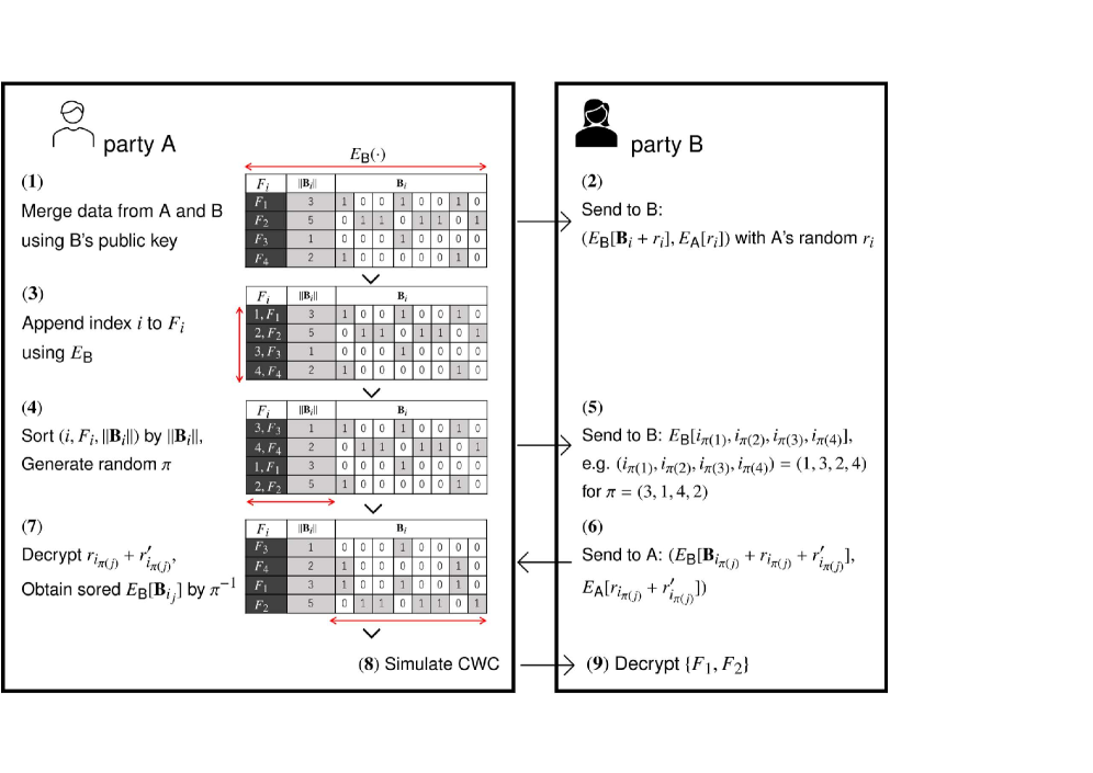
Figure 1: An example run of Algorithm 2. For simplicity, we omit the clock time in each ciphertext. (1): Parties A and B jointly compute $\mathbf{B}_{i}$ and $\|\mathbf{B}_{i}\|$ for each feature $F_{i}$ (same as the baseline algorithm). (2): A securely sends $\mathbf{B}_{i}$; B cannot learn anything. (3): A appends encrypted index $i$ for each $F_{i}$. (4): A sorts only $(F_{i},\|\mathbf{B}_{i}\|)$ by $\|\mathbf{B}_{i}\|$. (5): A sends the sorted indices with random permutation; B cannot learn anything. (6): B sends $\mathbf{B}_{i}$; A cannot learn anything from it. (7): A decrypts the noise and obtain the correct order of ${\mathbf{B}}_{i_{j}}$; A cannot learn anything. (8): A simulates CWC same as the baseline. (9): Party $\textsf{A},\textsf{B}$ share the resulting features.

Sorting is a major bottleneck for private CWC. The reason for this is that pointers cannot be moved across ciphertexts. For example, consider the case of secure integer sort. Let the variables $x$ and $y$ contain integers $a$ and $b$, respectively. In this case, by performing the secure operation $a<?b$, the result is obtained as $a<?b=c\in\{0,1\}$. Using this logical bit $c$, we can swap the values of $x$ and $y$ in $O(1)$ time satisfying $x<y$ by the secure operation $x\leftarrow c\cdot a+\bar{c}\cdot b$ and $y\leftarrow\bar{c}\cdot a+c\cdot b$.

In the case of CWC; however, each integer $i$ of feature $F_{i}$ is associated with the bit string $\mathbf{B}_{i}$. Since any $x$ cannot be decrypted, we cannot swap the pointers appropriately. Therefore, the baseline algorithm swaps $\mathbf{B}_{i}$ explicitly. As a result, the computation time for sorting increases to $O(mnk\log^{2}k)$. Our main contribution of this study is to improve this complexity to $O(mnk+k\log^{2}k)$ by reducing the cost for such explicit sorting.

Based on the FHE, we propose the improved secure CWC (Algorithm 2), which reduces the time complexity to $O(mnk+k\log^{2}k)$. An example run of Algorithm 2 is illustrated in Fig. 1. As shown in this example, the party A can securely sort $k$ randomized features in $O(k\log^{2}k)$ time using a suitable sorting network, and then, according to the result of sorting, A swaps each associated bit string of length $nm$ in $O(kmn)$ time. Following this preprocessing, the parties securely obtain minimal consistent features by decrypting the output of CWC. Finally, we get the following result.

Theorem 2

Algorithm 2 can simulate CWC in $O(kmn+k\log^{2}k+k\log k\log mn)$ time and $O(kmn)$ space under the assumption that FHE executes each bit operation in $O(1)$ time.

• Compared to the baseline, the additional space is required for $\pi$ and $r_{i}$ and $r^{\prime}_{i}$. Thus, the space complexity remains $O(kmn)$. For the time complexity, the main task is to sort $k$-triple $(F_{i},\|\mathbf{B}_{i}\|,\mathbf{B}_{i})$ in the increasing order of $\|\mathbf{B}_{i}\|$. The improved algorithm sorts only the pairs $x_{i}=(F_{i},\|\mathbf{B}_{i}\|)$ of integers, where the size of $x_{i}$ is $O(\log k+\log mn)$ bits. For each $x_{i},x_{j}$, we can check if $\|\mathbf{B}_{i}\|\leq\|\mathbf{B}_{j}\|$ in $O(\log mn)$ time and we can swap them in $O(\log k+\log mn)$ time using homomorphic operations in FHE. It follows that the time for sorting all $x_{i}$ $(i=1,\ldots,k)$ is $O(k\log k(\log k+\log mn))$ time. After sorting the pairs, the algorithm moves all $\mathbf{B}_{i}$ to the correct positions according to the rank of $x_{i}$ $(i=1,\ldots,k)$. This cost is $O(kmn)$. Therefore, time complexity is $O(kmn+k\log^{2}k+k\log k\log mn)$. $\Box$

Theorem 3

Algorithm 2 is secure under the assumption that the employed FHE is IND-CPA secure.

• We show the security by constructing simulators for parties A and B, respectively.

  B’s view (what B can obtain from A) is the following:

  • $(E_{\textsf{B}}[{\mathbf{B}}_{i}+r_{i}|1],E_{\textsf{A}}[r_{i}|1])$ for $i=1,\ldots,n$;

  • $E_{\textsf{B}}[i_{\pi(1)}|3],\ldots,E_{\textsf{B}}[i_{\pi(n)}|3]$.

  Their probability distributions are uniform and independent of each other. Hence, the simulator for B can replace them with

  • $(E_{\textsf{B}}[\mathbf{B}_{i}+r^{\prime\prime}_{i}|6],E_{\textsf{A}}[r^{\prime\prime}_{i}|6])$ for $i=1,\ldots,n$ and $r^{\prime\prime}_{i}$, which are selected uniformly at random;

  • $E_{\textsf{B}}[\pi^{\prime}(1)|6],\ldots,E_{\textsf{B}}[\pi^{\prime}(n)|6]$ for $\pi^{\prime}\in\mathfrak{S}_{n}$, which is selected uniformly at random.

  Note that, even if an adversary knows $\mathbf{B}_{i}$, it is computationally impossible to distinguish between $E_{\textsf{B}}[\mathbf{B}_{i}+r^{\prime\prime}_{i}|6]$ and $E_{\textsf{B}}[r^{\prime\prime}_{i}|6]$ by the IND-CPA security of the cryptosystem $E_{\textsf{B}}$.

  Next, we construct a simulator Sim for the party A. Although what A can obtain from B is

  $$\left\{\left.\left(E_{\textsf{B}}[{\mathbf{B}}_{i_{\pi(j)}}+r_{i_{\pi(j)}}+r^{\prime}_{i_{\pi(j)}}|4],E_{\textsf{A}}[r_{i_{\pi(j)}}+r^{\prime}_{i_{\pi(j)}}|4]\right)\right|j=1,\ldots,n\right\}$$

  this is equivalent to $\{E_{\textsf{B}}[{\mathbf{B}_{i_{j}}}|5]\mid j=1,\ldots,n\}$ after decryption and permutation.

  On the other hand, the sequence $(i_{1},\ldots,i_{n})$ is not explicitly given to A, and A recognizes it through the alignment between

  • $(E_{\textsf{B}}[\|{\mathbf{B}}_{i_{1}}\||3],\ldots,E_{\textsf{B}}[\|{\mathbf{B}}_{i_{n}}\||3])$ and

  • $(E_{\textsf{B}}[{\mathbf{B}}_{i_{1}}|5],\ldots,E_{\textsf{B}}[{\mathbf{B}}_{i_{n}}|5])$.

  Therefore, we define A’s view to be

  $${\tt View}_{\textsf{A}}=\left\{\left.\left(E_{\textsf{B}}[\|{\mathbf{B}}_{i_{j}}\||3],E_{\textsf{B}}[{\mathbf{B}}_{i_{j}})|5]\right)\right|j=1,\ldots,n\right\}$$

  with $\|{\mathbf{B}}_{i_{1}}\|\leq\cdots\leq\|{\mathbf{B}}_{i_{n}}\|$.

  On the other hand, we define the view that ${\tt Sim}$ should generate as follows: While A can generate $\{E_{\textsf{B}}[\|{\mathbf{B}}_{i_{j}}\||3]\mid j=1,\ldots,n\}$ with $\|{\mathbf{B}}_{i_{1}}\|\leq\cdots\leq\|{\mathbf{B}}_{i_{2}}\|$, A needs B’s cooperation to generate $\{E_{\textsf{B}}[{\mathbf{B}}_{i_{j}}|5]\mid j=1,\ldots,n\}$. Without B’s cooperation, ${\tt Sim}$ selects $\pi^{\prime}\in\mathfrak{S}_{n}$ uniformly at random, and generates its own view to be

  $${\tt View}_{\tt Sim}=\left\{\left.\left(E_{\textsf{B}}[\|{\mathbf{B}}_{i_{j}}\||3],E_{\textsf{B}}[{\mathbf{B}}_{\pi^{\prime\prime}(j)}|*]\right)\right|j=1,\ldots,n\right\}.$$

  Sim can compute $E_{\textsf{B}}[{\mathbf{B}}_{\pi^{\prime\prime}(j)}|*]$ from $E_{\textsf{B}}[0|*]$ and $E_{\textsf{B}}[{\mathbf{B}}_{\pi^{\prime\prime}(j)}|0]$ taking advantage of the homomorphic property of the encryption system $E_{\textsf{B}}$.

  Furthermore, we define a distinguisher $\cal D$ as a PPT Turing machine which tries to distinguish between ${\tt View}_{\textsf{A}}$ and ${\tt View}_{\tt Sim}$ on input of $\{(E_{\textsf{B}}[\|{\mathbf{B}}_{i}\||0],E_{\textsf{B}}[{\mathbf{B}}_{i}|0])\mid i=1,\ldots,n\}.$

  When we let $\Pr[Y=\textsf{A}\mid X=\textsf{A}]=1/2+\alpha_{1}$ and $\Pr[Y={\tt Sim}\mid X={\tt Sim}]=1/2+\alpha_{2}$, the advantage of $\cal D$ is defined as $\alpha_{1}+\alpha_{2}$.

  We show that , if $\cal D$’s advantage $\alpha$ is not negligible, we can construct a PPT attacker ${\tt Attck}$ that can brake the IND-CPA security of the encryption system $E_{\textsf{B}}$ with non-negligible advantage. Our attacker ${\tt Attck}$ plays the IND-CPA game exploiting an oracle ${\cal O}_{\text{IND}}$ as follows:

  1. ${\tt Attck}$ generates ${\mathbf{B}}_{1},{\mathbf{B}}_{2}$ with $\|{\mathbf{B}}_{1}\|\leq\|{\mathbf{B}}_{2}\|$;

  2. ${\tt Attck}$ lets $x_{1}=\|{\mathbf{B}}_{1}\|$ and $x_{2}=\|{\mathbf{B}}_{2}\|$ and throws a query $(x_{1},x_{2})$ to ${\cal O}_{\text{IND}}$;

  3. ${\cal O}_{\text{IND}}$ selects $i\in\{1,2\}$ uniformly at random and sends $c=E_{\textsf{B}}[x_{i}|-1]$ to ${\tt Attck}$;

  4. ${\tt Attck}$ initializes $\cal D$ by inputting $(E_{\textsf{B}}[\|{\mathbf{B}}_{1}\||0],E_{\textsf{B}}[\|{\mathbf{B}}_{1}\||0]),(E_{\textsf{B}}[\|{\mathbf{B}}_{2}\||0],E_{\textsf{B}}[\|{\mathbf{B}}_{2}\||0])$;

  5. First query. ${\tt Attck}$ throws to $\cal D$ the query: $(E_{\textsf{B}}[\|{\mathbf{B}}_{2}\||2],c),(E_{\textsf{B}}[\|{\mathbf{B}}_{2}\||2],E_{\textsf{B}}[{\mathbf{B}}_{2}|2])$;

  6. If $\cal D$ replies with A, ${\tt Attck}$ outputs $1$ and terminates.

  7. Second query. ${\tt Attck}$ generates $c^{\prime}$ by adding $E_{\textsf{B}}[0|3]$ to $c$. Note that ${\cal D}_{\textsf{B}}(c^{\prime})={\cal D}_{\textsf{B}}(c)$ holds. ${\tt Attck}$ throws to $\cal D$ the query: $(E_{\textsf{B}}[\|{\mathbf{B}}_{1}\||3],E_{\textsf{B}}[{\mathbf{B}}_{2}|3]),(E_{\textsf{B}}[\|{\mathbf{B}}_{2}\||3],c^{\prime})$.

  8. If $\cal D$ replies with ${\tt Sim}$, ${\tt Attck}$ outputs $1$ and terminates.

  9. ${\tt Attck}$ outputs $2$.

  We evaluate ${\tt Attck}$’s advantage as follows. We assume ${\cal D}_{\textsf{B}}(c)=x_{1}$. The probability of this case is $1/2$. The probability that $\cal D$ replies with A to the first query or $\cal D$ replies with ${\tt Sim}$ to the second query is

  $$\frac{1}{2}+\alpha_{1}+\frac{1}{2}+\alpha_{2}-(\frac{1}{2}+\alpha_{1})(\frac{1}{2}+\alpha_{2})=\frac{3}{4}+\frac{\alpha}{2}-\alpha_{1}\alpha_{2}\geq\frac{3}{4}+\frac{\alpha}{4},$$

  since the first and second queries are mutually independent.

  When assuming $D_{B}(c)=x_{2}$, we see that $\Pr[\text{$\cal D$ outputs ${\tt Sim}$ at the first query }]-1/2$ is negligible. Otherwise, $\cal D$ can be used as an attacker to break the IND-CPA security of $E_{B}$. Therefore, $\Pr[{\text{{Attck} outputs 2}}]-1/4$ is negligible. Consequently, we have

  $$\Pr[\text{${\tt Attck}$'s guess is right}]\geq\frac{1}{2}\left(\frac{3}{4}+\frac{\alpha}{4}\right)+\frac{1}{2}\cdot\frac{1}{4}=\frac{1}{2}+\frac{\alpha}{8}.$$

  Since we assume that $\alpha$ is not negligible, neither is $\alpha/4$. $\Box$

4 Experiments

We implemented the baseline and improved algorithms for secure CWC in C++ using TFHE library. The experiments were carried out on a machine equipped with Intel Core i7-6567U (3.30GHz) processor and 16GB of RAM. In the following, $m$ (resp. $n$) is the number of positive (resp. negative) data and $k$ is the number of features.

Table 6 summarizes the running time of the baseline algorithm (naive implementation of Algorithm 1 using TFHE) for random data generated for $k\in\{10,50,100\}$ and $mn\in\{100,500,1000\}$. The complexity analysis shows that the running time increases in proportion to $mn$. This experimental result confirms this in real data. The table clearly shows that the sorting process is the bottleneck.

Table 6: Running time (sec) of baseline algorithm (naive secure CWC). Task 1: computing $\mathbf{B}_{i}$’s. Task 2: sorting $\mathbf{B}_{i}$’s. Task 3: feature selection.

$k$	$mn$	Task 1	Task 2	Task 3
	100	60.3	835.8	111.9
10	500	300.5	4,252.4	558.1
	1,000	601.4	8,867.0	1,114.2
	100	301.8	6,292.6	589.3
50	500	1,502.9	30,364.6	2,941.0
	1,000	3,007.0	62,124.6	5,919.7
	100	603.7	16,148.5	1,179.0
100	500	3,005.9	76,315.2	5,952.5
	1,000	6,014.1	154,143.5	11,867.0

Table 7 compares the running time of preprocessing in baseline and improved algorithms. According to the results, the proposed algorithm significantly improves the bottleneck in naive CWC for secure computing. We should note that baseline and improved algorithms both compute exactly the same solution as the CWC on plaintexts. We also show the details of improved algorithm: ‘sorting’ means the time for sorting of the triples $(F_{i},||{\mathbf{B}}_{i}||,i)$ of integers. ‘other task’ means the time for remaining tasks including generating/adding/subtracting random noise $r_{i}$, moving ${\mathbf{B}}_{i}$, decrypting integers, etc.

Table 7: Running time (sec) of baseline and improved algorithms. ‘baseline’ is same as Task 2 in Table 6 (i.e. the bottleneck). ‘improved:’ is the running time of corresponding task in the improved algorithm, where ‘sorting’ and ‘other tasks’ are the details.

$k$	$mn$	baseline	improved:	sorting	other tasks
	100	835.8	203.7	69.4	134.2
10	500	4,252.4	286.2	89.5	196.6
	1000	8,867.0	302.5	98.9	203.6
	100	16,148.5	3,311.2	1,865.5	1,445.7
100	500	76,315.2	4,601.9	2,647.7	1,954.1
	1000	154,143.5	4,671.4	2,660.8	2,010.5

Table 8 displays the running time of improved algorithm for real data available from UCI Machine Learning Repository, because since these datasets contain more than three feature/class values, we treated them as a binary classification between one feature/class and the other.

Table 8: Running time (sec) of improved algorithm for real data in UCI Machine Learning Repository.

dataset	$k$	$mn$	time	sorting	other tasks
Letter	16	196	252.2	80.6	171.4
Breast Cancer	10	2,464	312.6	103.1	209.5
Covertype	54	979	1,653.5	836.9	816.6

We demonstrated that the proposed algorithm works well for real-world multi-level feature selection problems. We only evaluated the running time in this experiment, but the relevance of the extracted features is guaranteed because the secure CWC algorithm produces the same solution as the original [2].

5 Conclusion

On the basis of fully homomorphic encryption, we proposed a faster private feature selection algorithm that allow us to securely compute functional features from distribute private datasets. Our algorithm can simulate the original CWC algorithm, which chooses favorable features by sorting. In addition to the improvement in computational complexity, the proposed algorithm solves the private feature selection problem in practical time for a variety of real data. One of the remaining challenges is to improve sorting at a lower cost because CWC does not always require exact sorting. Then, ambiguous sorting possibly reduces the computation time maintaining solution quality. At this time, the proposed algorithm is not applicable to real number for feature value. This is because TFHE is not good at floating point operations. Extending the TFHE library to enable secure feature selection for real-valued data is a future challenge.

References

- [1] Shin, K.; Kuboyama, T.; Hashimoto, T.; Shepard, D. SCWC/SLCC: Highly scalable feature selection algorithms. Information 2017 8(4), 159.
- [2] Shin, K.; Xu, X.M. Consistency-based feature selection. In Proceedings of 13th International Conference on Knowledge-Based and Intelligent Information and Engineering Systems, Santiago, Chile, 28-30 September 2009, pp.28–30.
- [3] Almuallim, H.; Dietteric, T.G. Learning boolean concepts in the presence of many irrelevant features. Artif. Intell. 1994 69(1-2), 279–30.
- [4] Liu, H.; Motoda, H.; Dash, M. A monotonic measure for optimal feature selection. In Proceedings of 10th European Conference on Machine Learning, Chemnitz, Germany, 21-23 April 1998, pp.101–106.
- [5] Shin, K.; Fernandes, D.; Miyazaki, D. Consistency measures for feature selection: A formal definition, relative sensitivity comparison, and a fast algorithm. In Proceedings of 22nd International Joint Conference on Artificial Intelligence, Barcelona, Spain, 16–22 July 2011, pp.1491–1497.
- [6] Zhao, Z.; Liu, H. Searching for interacting features. In Proceedings of 20th International Joint Conference on Artificial Intelligence, Hyderabad, India, 6-12 January 2007, pp.1156–1161.
- [7] Paillier, P. Public-key cryptosystems based on composite degree residuosity classes. In Proceedings of International Conference on the Theory and Application of Cryptographic Techniques, Prague, Czech Republic, 2-6 May 1999, pp.223–238.
- [8] Attrapadung, N.; Hanaoka, G.; Mitsunari, S.; Sakai, Y.; Shimizu, K.; Teruya, T. Efficient two-level homomorphic encryption in prime-order bilinear groups and a fast implementation in webassembly. In Proceedings of the 2018 on Asia Conference on Computer and Communications Security, Incheon, Republic of Korea, 4 June 2018, pp.685–697.
- [9] Boneh, D.; Goh, E.J.; Nissim, K. Evaluating 2-DNF formulas on ciphertexts. In Proceedings of Theory of Cryptography Conference, Cambridge, MA, USA, 10-12 February 2005, pp.325–341.
- [10] Brakerski, Z.; Gentry, C.; Vaikuntanathan, V. (leveled) fully homomorphic encryption without bootstrapping. Proceedings of 3rd Innovations in Theoretical Computer Science, Cambridge, MA, USA, 8-10 January 2012, pp.309–325.
- [11] Gentry, C. Fully homomorphic encryption using ideal lattices. In Proceedings of the 41st ACM Symposium on Theory of Computing, Bethesda, MD, USA, 31 May - 2 June 2009, pp.169–178.
- [12] Chillotti, I.; Gama, N.; Georgieva, M.; Izabachène, M. TFHE: Fast fully homomorphic encryptionover the torus. Journal of Cryptology 2020 33, 34–-91.
- [13] Chillotti, I.; Gama, N.; Georgieva, M.; Izabachène, M. TFHE: Fast fully homomorphic encryption library, August 2016. https://tfhe.github.io/tfhe
- [14] Goldwasser, S.; Micali, S. Probabilistic Encryption. Journal of Computer and System Sciences 1984 28(2), 270–299.
- [15] Fujisaki, E.; Okamoto, T.; Pointcheval, D.; Stern, J. RSA-OAEP is secure under the RSA assumption. In Proceedings of the 21st Annual International Cryptology Conference, Santa Barbara, California, USA, 19-23 August 2001, 260–274.
- [16] Bellare, M.; Rogaway, P. Optimal Asymmetric Encryption. In Proceedings of Workshop on the Theory and Application of Cryptographic Techniques, Perugia, Italy, 9-12 May 1994, 92–111.
- [17] Rao, V.; Long, Y.; Eldardiry, H.; Rane, S.; Rossi, R.A.; Torres, F. Secure two-party feature selection. arXiv, 1901.00832, 2019.
- [18] Anarakia, J.R.; Samet, S. Privacy-preserving feature selection: A survey and proposing a new set of protocols. arXiv, 2008.07664, 2020.
- [19] Banerjee, M.; Chakravarty, S. Privacy preserving feature selection for distributed data using virtual dimension. Proceedings of the 20th ACM international conference on Information and knowledge management, Glasgow Scotland, UK, 24 - 28 October 2011, pp.2281–-2284.
- [20] Sheikhalishahi, M.; Martinelli, F. Privacy-utility feature selection as a privacy mechanism in collaborative data classification. Proceedings of the 26th International Conference on Enabling Technologies: Infrastructure for Collaborative Enterprises, Poznan, Poland, 21 –23 June 2017, pp.244–-249.
- [21] Li, X.; Dowsley, R.; Cock, M.D. Privacy-preserving feature selection with secure multiparty computation. In Proceedings of the 38th International Conference on Machine Learning, online, 18 - 24 July 2021, pp.6326–6336.
- [22] Abspoel, M.; Escudero, D.; Volgushev, N. Secure training of decision trees with continuous attribute. Proc. Priv. Enhancing Technol. 2021 2021(1), 167–187.
- [23] Ajtai, M.; Szemerédi, E.; Komlós, J. An sorting network. Proceedings of the 15th Annual ACM Symposium on Theory of Computing, Boston, Massachusetts, USA, 25-27 April 1983, pp.1–9.
- [24] Batcher, K.E. Sorting networks and their applications. In Proceedings of American Federation of Information Processing Societies (AFIPS) Spring Joint Computing Conference, Atlantic City, NJ, USA, 30 April - 2 May 1968, 307–314.
- [25] Hamada, K.; Chida, K.; Ikarashi, D.; Takahashi, K. Oblivious radix sort: An efficient sorting algorithm for practical secure multi-party computation. IACR Cryptol. ePrint Arch. 2014 121.
- [26] Sampigethaya, K.; Poovendran, R. A survey on mix networks and their secure applications. Proceedings of the IEEE 2006 94(12), 2142–2181.