Holographic beam shaping of partially coherent light

Abstract

We present an algorithm for holographic shaping of partially coherent light, bridging the gap between traditional coherent and geometric optical approaches. The description of partially coherent light relies on a mode expansion formalism, with possibly thousands of individual modes, and the inverse-design optimization algorithm is based on gradient descent with the help of algorithmic differentiation. We demonstrate numerically and experimentally that an optical system consisting of two phase patterns can potentially achieve any intensity profile transformation with good accuracy.

Sculpting light freely into user-defined shapes is a central key aspect in many areas of photonics. The list of fields with a strong interest in beam shaping is extensive and ranges from applied areas such as laser material processing [1, 2, 3, 4], mode conversion [5], near-eye displays [6], lithography, telecommunications and practical lighting systems to fundamental research in biology and physics, such as investigations towards revealing the functioning of the brain via patterned photostimulation [7] or the trapping of microparticles [8] and atoms [9]. Complex spatial wavefronts can be shaped using either static components such as diffractive optical elements (DOEs), freeform elements [10] and metasurfaces [11], or dynamic devices like spatial light modulators (SLM) based on liquid crystal, micro electromechanical systems (MEMS) technology, or even soundwaves [12].

Despite the prowess of today’s beam shaping technology, there remain important challenges. One of them is tailoring fields with a lack of coherence, i.e. partially coherent or incoherent light, which is of central importance in many lighting and high power laser applications. In particular configurations, where light sources satisfy the geometric optical regime, some solutions based on ray-optical approaches have proven to be efficient [13, 14]. The main advantage of such approaches is that they enforce the design of surfaces with curl-free gradients that are perfectly adapted to freeform elements. However, these methods inherently neglect diffraction and are therefore ill-suited for applications involving miniaturized integrated optics [15] or multicolor beam shaping [16, 17, 6], as well as for applications requiring more complex partially coherent sources.

Usual representations of partially coherent light introduce 4-dimensional second-order correlation functions [18], like the mutual coherence function or the mutual intensity function in the quasi-monochromatic case, in order to accurately describe the statistical nature of light fields seen as random processes. Such 4D correlation functions admit, due to Mercer’s theorem, a mode expansion consisting of spatially coherent and mutually uncorrelated fields. Although it is also admitted that computing such mode expansions is in general a hard task, as it involves solving the eigenvalues of a Fredholm integral equation, some ubiquitous light sources like multimode lasers or multimode fibers already exhibit eigen-modes as the basis of their physical description. Moreover, for different types of sources, it is often possible to find some phenomenological approximate models that provide convenient analytical modal descriptions, for instance in the same way as we proceed in the following to model a light-emitting diode (LED) source.

In this article we present a novel algorithmic approach, which allows the efficient design of multiple phase-only DOEs for shaping user defined intensity distributions of partially coherent light, as described above in terms of spatially coherent and mutually uncorrelated modes. The approach employs numerical wave propagation and is not limited by any geometric constraints such as rotational symmetry. Its only limitation lies in the thin element approximation (TEA) which must hold for the experimental realization. For the sake of generality, we provide an algorithm that accounts for an arbitrary number of DOEs, although we show later that two phase patterns are sufficient in all the situations we considered, to obtain nearly perfect intensity shaping. Moreover, we experimentally demonstrate the concept by redistributing a part of the light from an LED into various shapes using two diffractive patterns displayed on a liquid crystal SLM. Given the widespread use of partially coherent sources in science and technology, we anticipate that our work will be helpful for the advancement of research fields concerned with tailored light fields.

The algorithm we developed consists of an optimization procedure relying on gradient descent in order to minimize the $l_{2}$ distance between the time-averaged transverse intensity profile $I_{S}$ of the partially coherent source after crossing the optical system and a user-defined target intensity profile $I_{T}$. Since we assume that the modes defining the partially coherent source are mutually uncorrelated, their time-averaged intensity $I_{S}$ is simply the sum of the contributions of all the individual modes constituting the source. The optimization procedure is iterative and consists of three stages. First, a forward pass propagates $n_{modes}$ input modes $U_{0}[1:n_{modes}]$ from the partially coherent source plane to the detection plane where the desired intensity profile $I_{T}$ is to be detected, through the optical system consisting of $n_{layers}$ longitudinally separated phase patterns $\Phi[1:n_{layers}]$. A pseudo-code description of the forward model is presented in algorithm 1. Second, the time-averaged input intensity $I_{S}$ is computed in the detection plane and serves to define an error value $err$ based on the $l_{2}$ distance between $I_{S}$ and $I_{T}$. Since the goal of the algorithm is to minimize this error with respect to the phase parameters $\Phi$, the gradient $\nabla_{\Phi}$ of this error has to be computed. To this end, we develop a backward pass, as is commonly done in computer science to numerically compute the gradients of complicated neural network architectures with gradient backpropagation algorithms. Here we used a few rules from the set defined in [19], leading to the error and gradient computation algorithm 2. Third, we need to update the phase patterns $\Phi$. Since we managed to compute a gradient, any first-order optimization method can be employed, the simplest being adding a small gradient step of opposite direction, $\Phi\leftarrow\Phi-\alpha\nabla_{\Phi}$ with $\alpha>0$. These three stages need to be repeated iteratively, until a convergence criterion regarding the error is achieved, $err<\epsilon$ with $\epsilon>0$.

Algorithm 1 Forward model

$\mathbf{Inputs:}$ $U_{0}$ a list of 2D input modes

$\mathbf{Inputs:}$ $\Phi$ a list of phase patterns

$\mathbf{Outputs:}$ $U$ a list of propagated modes

$\mathbf{Outputs:}$ $S$ a list of modes stored in each plane

procedure propagate_forward($U_{0}$, $\Phi$)

     $U\leftarrow\textsc{copy}(U_{0})$ $\triangleright$ copy initialization

     $S\leftarrow\textsc{Modes\_List}(n_{layers})$ $\triangleright$ empty initialization

     for $l=1\,\mathbf{to}\,n_{layers}$ do

         $U\leftarrow\textsc{prop.}(U,l)$ $\triangleright$ propagating modes to plane $l$

         $U\leftarrow U\cdot\exp{(i\Phi[l])}$ $\triangleright$ crossing $l$^th DOE forward

         $S[l]\leftarrow U$ $\triangleright$ storing modes at plane $l$

     end for

     $U\leftarrow$ FFT.($U$) $\triangleright$ propagating to detection plane

     return $(U,S)$

end procedure

In algorithm 1, the inputs of the propagate_forward procedure are $U_{0}$, a list of $n_{modes}$ transverse modes mutually uncorrelated constituting the partially coherent source, and $\Phi$ a list of $n_{layers}$ phase patterns initially set to flat phases. The outputs are $U$, a list of modes propagated to the detection plane, and $S$, a list of modes stored just after crossing each phase pattern which will be essential to compute the backpropagated gradient later on. More precisely, $S$ is a list of a list, the outer list being of length $n_{layers}$ and storing inner lists of modes of length $n_{modes}$. The data structures present in the algorithms are defined in order to simplify the notations and provide conciseness, but do not prejudge how they should be implemented in practice in order to get the best performance. In order to avoid verbose loops on the mode index, we present the code in a vectorized form by appending a dot (.) after the functions that we want to broadcast over the different elements of a list type parameter. Similarly, the vectorized point-wise multiplication of a collection of modes with a single phase pattern is defined by a dot operator ($\cdot$). To describe mode propagation from its current plane definition to a phase pattern plane of index $l$, we introduce a generic prop function, taking both a tranverse mode and an index $l$ as parameters, which can be defined according to the user’s choice. A simple model that we also use in the current study is the Angular Spectrum (AS) method for free-space propagation and Fast Fourier Transform (FFT) for Fourier collimation or focusing. In the forward model description 1 as well as in our following experimental demonstration, we choose the detection plane to be Fourier-conjugated to the last phase pattern of the optical system, but this is again arbitrary, up to the user’s choice.

Algorithm 2 Error and gradient computation

$\mathbf{Inputs:}$ $U$ a list of propagated modes

$\mathbf{Inputs:}$ $S$ a list of modes stored in each plane

$\mathbf{Inputs:}$ $\Phi$ a list of phase patterns

$\mathbf{Inputs:}$ $I_{T}$ a target intensity profile

$\mathbf{Outputs:}$ $err$ an error associated with the forward model $\mathbf{Outputs:}$ $\nabla_{\Phi}$ a list of phase gradients

procedure backpropagate_gradient($U$, $S$, $\Phi$, $I_{T}$)

     $I_{S}\leftarrow\sum\limits_{m=1}^{n_{modes}}|U[m]|^{2}$ $\triangleright$ storing source intensity

     $err\leftarrow{\displaystyle\int}{\left(I_{S}-I_{T}\right)^{2}}$ $\triangleright$ computing the error value

     $\nabla_{\Phi}\leftarrow\textsc{Phase\_List}(n_{layers})$ $\triangleright$ empty initialization

     $U\leftarrow 4\left(I_{S}-I_{T}\right)\cdot U$

     $U\leftarrow\textsc{IFFT.}(U)$ $\triangleright$ backpropagating to the last DOE

     for $l=n_{layers}\,\mathbf{to}\,1$ do

         $\nabla_{\Phi}[l]\leftarrow\Im{\left(\sum\limits_{m=1}^{n_{modes}}(S^{*}[l]\cdot U)[m]\right)}$ $\triangleright$ $l$^th phase gradient

         $U\leftarrow U\cdot\exp{(-i\Phi[l])}$ $\triangleright$ crossing $l$^th DOE backward

         $U\leftarrow\textsc{prop.*}(U,l)$ $\triangleright$ propagating backward

     end for

end procedure

return $(err,\nabla_{\Phi})$

The algorithm 2 describes the error and gradients computation which are returned by the backpropagate_gradient procedure. The list of propagated fields $U$ returned by the forward propagation procedure is used to compute the error $err$ and is backpropagated in a mirrored fashion through the same optical system. In order to achieve gradient backpropagation, all the propagation operators need to be replaced by their adjoint (Hermitian conjugate) operators denoted by an asterisk (^∗). Moreover, it is important to notice that the gradient computation $\nabla_{\Phi}[l]$ associated to each individual phase pattern $\Phi[l]$ occurs in reverse order and depends only on the modes stored in $S[l]$ during the forward pass and on the modes $U$ backpropagated to the same plane $l$.

We experimentally demonstrate the performance and accuracy of our beam shaping algorithm by implementing the setup shown in Fig. 1. A single SLM (Hamamatsu X10468, $16$ mm $\times$ $12$ mm) and a mirror (square with 5 mm side length) form a tandem configuration of two diffractive patterns. Similar layouts have been used in the past for shaping coherent light and approaching properties of volume holograms, such as wavelength and angular selectivity [20, 21, 22, 17, 23, 24]. Our approach is conceptually related, however, our algorithm is different and the number of modes it manages to handle in order to accurately describe partially coherent light is substantially higher compared to the previous state of the art (up to 1600 individual coherent modes shown in this letter), which is an essential prerequisite for realizing practical application cases.

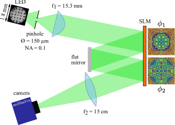
Figure 1: Folded setup for holographic beam shaping with 2 reflections on a single SLM.

In this proof of concept study, we employ a green LED (Thorlabs M530L4) as a primary source, with a peak emission wavelength around $522$ nm and $35$ nm bandwidth. The emitter is square-shaped with 1 mm side length with a plastic dome affixed on the top that modifies the spatial emission characteristics. Following a pragmatic approach, we incorporate the optical effects of the plastic dome by modelling the LED according to its image through a 1:1 Keplerian telescope (NA = 0.25), where the emitter appears to be roughly circular with a radius of $r_{0}=900$ µm, exhibiting several dark spots arranged in a square pattern. In our algorithm, we use this image as a replacement for the true LED plus the dome lens. The LED light is filtered by a pinhole of radius $r_{pin}=75$ µm, which is positioned at a distance $z_{pin}$ from the LED such that the numerical aperture (NA) of the light passing through it is about $\textrm{NA}\simeq 0.1$. After collimation by a first lens (focal length $f_{1}$ = 15.3 mm), the beam radius is measured to be $r_{col}=1625$ µm. After collimation, the light traverses two diffractive patterns, $\Phi_{1}$ and $\Phi_{2}$, at distances of 165 mm and 325 mm from the collimating lens, respectively. Finally, it is directed onto a camera by a second lens ($f_{2}$ = 15 cm) at a distance $f_{2}$ from the sensor. Therefore, the camera captures a magnified image of the aperture ($\approx\times 10$) if no diffractive patterns are shown.

From the simulation point of view, we treat the LED as a totally incoherent light source [25]. We discretize the LED emitter model into a square grid of size $N_{S}\times N_{S}$, which determines the number of uncorrelated modes representing our source. The pixel size $dx_{S}=dy_{S}$ in each dimension is chosen such that the total grid side length is $2r_{0}$, and the source profile is idealized to a disc of radius $r_{0}$ with constant intensity. Then, each pixel acts as an independent spherical wave source with an amplitude proportional to the square root of the local intensity, $\sqrt{I}e^{ikr}/r$, that propagates to the pinhole plane where it is clipped by the 150 µm diameter aperture. Thus, the analytical expression of each transverse mode is known in the pinhole plane and serves to define $N_{S}^{2}$ input distributions stored in grids of size $512\times 512$ with a pixel size $dx_{pin}=dy_{pin}=1$ µm. The collimation of the input modes by the lens following the pinhole is modeled via a scaled FFT (Chirp Z-transform), and the resolution after collimation is set to $dx=dy=20$ µm, which directly matches the SLM pixel size. Obviously, given our disc shape model of the LED, some of the generated modes have zero intensity and could be removed for optimizing memory and computation time (the number of effectively used modes is about $\pi N_{S}^{2}/4$).

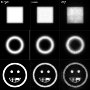
Figure 2: Results of the beam shaping algorithm with 2 phase patterns for 3 different target intensity profiles (square, ring, smiley). The first column represents the target intensity profiles set as inputs of the simulation. The second column shows the simulated intensity profiles and the third column shows the intensity profiles recorded on a camera when the phase patterns computed by the simulation are displayed on the SLM.

The results of the beam shaping algorithm with two phase patterns are displayed in Fig. 2. We chose $N_{S}=40$ corresponding to 1600 modes. In order to demonstrate the flexibility of the algorithm, the LED emission is sculpted into three different shapes: a square of 1.5 mm side length, a Gaussian ring with $675$ µm radius and $150$ µm waist, and a smiley containing fine details with 2.3 mm outer diameter. The simulations show an excellent agreement with the theoretical target intensity profiles, which are obtained after a few hundreds of iterations associated to an error bound $\epsilon=1.10^{-8}$, for targets of total intensity normalized to unity. The typical computation time for such precision is about 10 minutes on a mid-range GPU (Geforce RTX 2070 Super). The experimental results obtained with setup 1 are likewise excellently matching the theoretical targets, even if we sometimes observe some weak modulations reminiscent of the LED substructure that we did not fully take into account. Moreover, we experimentally observe that our multimode holographic transformations are much less sensitive to misalignment than similar shaping of coherent light, where noticeable speckle usually appears even for small misalignments.

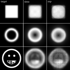
Figure 3: Results of the beam shaping algorithm with 1 phase pattern for the same targets as in figure 2.

Our simulations and experiments demonstrate that two phase patterns are sufficient to obtain nearly perfect intensity shaping of an incoherent source such as an LED. We performed further simulations considering different mode bases suitable for describing several other partially incoherent light sources, such as Hermite-Gaussian (HG) or Linearly Polarized (LP) modes, obtaining similar quality levels for all cases (data not shown).

Next we show that these complicated beam transformations cannot be achieved by a single phase pattern. For this purpose we enforce $\Phi_{1}$ to remain flat, thus only relying on $\Phi_{2}$ to achieve the same transformations as above. The results displayed in Fig. 3 confirm that one phase pattern is not sufficient to ensure a good convergence of the algorithm to the defined targets. Notably, we still observe a good agreement between simulations and experimental results.

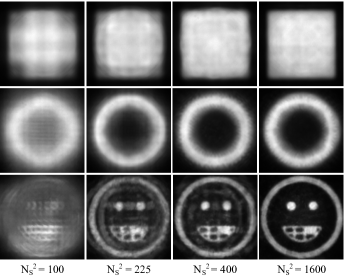
Figure 4: Evolution of the experimental intensity profiles with respect to the number of modes involved in the modeling of the input beam.

Finally, it is important to discuss the impact of the number of modes used for source modeling on the reconstruction quality. Regardless the number of modes, the simulation always converges almost perfectly to the given target intensity, but severely undercutting the number of modes required to accurately describe the light source significantly degrades the result. Figure 4 visualizes the influence of the mode number on the quality of the experimental intensity shaping. An upper bound for the number of modes required to represent our light source can be estimated using Shannon’s sampling theorem. The maximally allowed spatial sampling distance for any object imaged at a given NA is $dx_{min}=\lambda/(2\textrm{NA})$. We can determine the maximum number of modes to be $n_{max}=\pi r_{pin}^{2}/dx_{min}^{2}$, which is close to $n_{max}=2600$ in our case. We managed to obtain a very good intensity fidelity with only about 1257 modes for our three profiles, but finer details or sharper edges in the target intensity profile may require an even higher number.

In conclusion, we presented a general algorithm designed to shape the intensity of partially coherent light, given its expansion in terms of coherent and mutually uncorrelated modes. We demonstrated the efficiency of this algorithm and evaluated it experimentally with a simple optical system consisting of two phase-only diffractive patterns, which appears sufficient to achieve a very good fidelity. Incorporating 1600 modes as presented in this work takes about 10 minutes of computation time. From this we can conclude that handling light sources of substantially higher complexity (e.g. 10$\times$ more modes) would readily work in a reasonable time on standard PC hardware. Therefore, we can envision extending this work to more complex situations such as the combination of several partially coherent beams, eventually with multiple colors, by adapting this algorithm to the design of multilayer or volumic DOEs.

Funding.

The work is funded by the FWF (I3984-N36).

References

- [1] T Häfner, J Strauß, C Roider, J Heberle, and M Schmidt. Tailored laser beam shaping for efficient and accurate microstructuring. Applied Physics A, 124(2):1–9, 2018.
- [2] Daniel Flamm, Daniel Günther Grossmann, Michael Jenne, Felix Zimmermann, Jonas Kleiner, Myriam Kaiser, Julian Hellstern, Christoph Tillkorn, and Malte Kumkar. Beam shaping for ultrafast materials processing. In Laser Resonators, Microresonators, and Beam Control XXI, volume 10904, page 109041G. International Society for Optics and Photonics, 2019.
- [3] Patrick S Salter and Martin J Booth. Adaptive optics in laser processing. Light: Science & Applications, 8(1):1–16, 2019.
- [4] Rongpei Shi, Saad A Khairallah, Tien T Roehling, Tae Wook Heo, Joseph T McKeown, and Manyalibo J Matthews. Microstructural control in metal laser powder bed fusion additive manufacturing using laser beam shaping strategy. Acta Materialia, 184:284–305, 2020.
- [5] Nicolas K Fontaine, Roland Ryf, Haoshuo Chen, David T Neilson, Kwangwoong Kim, and Joel Carpenter. Laguerre-gaussian mode sorter. Nature Communications, 10(1):1–7, 2019.
- [6] Praneeth Chakravarthula, Yifan Peng, Joel Kollin, Henry Fuchs, and Felix Heide. Wirtinger holography for near-eye displays. ACM Transactions on Graphics (TOG), 38(6):1–13, 2019.
- [7] Emiliano Ronzitti, Cathie Ventalon, Marco Canepari, Benoît C Forget, Eirini Papagiakoumou, and Valentina Emiliani. Recent advances in patterned photostimulation for optogenetics. Journal of Optics, 19(11):113001, 2017.
- [8] E Otte and C Denz. Optical trapping gets structure: structured light for advanced optical manipulation. Applied Physics Reviews, 7(4):041308, 2020.
- [9] Daniel Barredo, Vincent Lienhard, Sylvain De Leseleuc, Thierry Lahaye, and Antoine Browaeys. Synthetic three-dimensional atomic structures assembled atom by atom. Nature, 561(7721):79–82, 2018.
- [10] Harald Ries and Julius Muschaweck. Tailored freeform optical surfaces. Journal of the Optical Society of America A, 19(3):590–595, Mar 2002.
- [11] Seyedeh Mahsa Kamali, Ehsan Arbabi, Amir Arbabi, and Andrei Faraon. A review of dielectric optical metasurfaces for wavefront control. Nanophotonics, 7(6):1041–1068, 2018.
- [12] Peter Bechtold, Ralph Hohenstein, and Michael Schmidt. Beam shaping and high-speed, cylinder-lens-free beam guiding using acousto-optical deflectors without additional compensation optics. Optics Express, 21(12):14627–14635, 2013.
- [13] Vladimir Oliker, Leonid L. Doskolovich, and Dmitry A. Bykov. Beam shaping with a plano-freeform lens pair. Optics Express, 26(15):19406–19419, Jul 2018.
- [14] ShiLi Wei, ZhengBo Zhu, ZiChao Fan, YiMing Yan, and DongLin Ma. Double freeform surfaces design for beam shaping with non-planar wavefront using an integrable ray mapping method. Optics Express, 27(19):26757–26771, Sep 2019.
- [15] Sören Schmidt, Simon Thiele, Andrea Toulouse, Christoph Bösel, Tobias Tiess, Alois Herkommer, Herbert Gross, and Harald Giessen. Tailored micro-optical freeform holograms for integrated complex beam shaping. Optica, 7(10):1279–1286, Oct 2020.
- [16] Alexander Jesacher, Stefan Bernet, and Monika Ritsch-Marte. Colour hologram projection with an slm by exploiting its full phase modulation range. Optics Express, 22(17):20530–20541, 2014.
- [17] Haiyan Wang and Rafael Piestun. Dynamic 2d implementation of 3d diffractive optics. Optica, 5(10):1220–1228, 2018.
- [18] Max Born and Emil Wolf. Principles of optics: electromagnetic theory of propagation, interference and diffraction of light. Elsevier, 2013.
- [19] Alden S. Jurling and James R. Fienup. Applications of algorithmic differentiation to phase retrieval algorithms. Journal of the Optical Society of America A, 31(7):1348–1359, Jul 2014.
- [20] Hartmut O. Bartelt. Applications of the tandem component: an element with optimum light efficiency. Applied Optics, 24(22):3811–3816, Nov 1985.
- [21] Stefan Borgsmüller, Steffen Noehte, Christoph Dietrich, Tobias Kresse, and Reinhard Männer. Computer-generated stratified diffractive optical elements. Applied Optics, 42(26):5274–5283, Sep 2003.
- [22] Alexander Jesacher, Christian Maurer, Andreas Schwaighofer, Stefan Bernet, and Monika Ritsch-Marte. Near-perfect hologram reconstruction with a spatial light modulator. Optics Express, 16(4):2597–2603, Feb 2008.
- [23] Stirling Scholes and Andrew Forbes. Improving the beam quality factor (M2) by phase-only reshaping of structured light. Optics Letters, 45(13):3753–3756, 2020.
- [24] Niyazi Ulas Dinc, Joowon Lim, Eirini Kakkava, Christophe Moser, and Demetri Psaltis. Computer generated optical volume elements by additive manufacturing. Nanophotonics, 9(13):4173–4181, 2020.
- [25] Yuanbo Deng and Daping Chu. Coherence properties of different light sources and their effect on the image sharpness and speckle of holographic displays. Scientific Reports, 7(1):1–12, 2017.