State Estimation Using a Network of Distributed Observers With Unknown Inputs

Abstract

State estimation for a class of linear time-invariant systems with distributed output measurements (distributed sensors) and unknown inputs is addressed in this paper. The objective is to design a network of observers such that the state vector of the entire system can be estimated, while each observer (or node) has access to only local output measurements that may not be sufficient on its own to reconstruct the entire system’s state. Existing results in the literature on distributed state estimation assume either that the system does not have inputs, or that all the system’s inputs are globally known to all the observers. Accordingly, we address this gap by proposing a distributed observer capable of estimating the overall system’s state in the presence of inputs, while each node only has limited local information on inputs and outputs. We provide a design method that guarantees convergence of the estimation errors under some mild joint detectability conditions. This design suits undirected communication graphs that may have switching topologies and also applies to strongly connected directed graphs. We also give existence conditions that harmonize with existing results on unknown input observers. Finally, simulation results verify the effectiveness of the proposed estimation scheme for various scenarios.

, , , and

1 Introduction

The increasing ubiquity of embedded systems has empowered sensing equipment with communication and computation capabilities that allow complex algorithms to be deployed on sensors themselves. This is especially beneficial for larger systems comprising many different components, whose state space has a significant size or is spread over a large area. Systems of this kind encompass smart buildings with many networked sensing points [1] or water and power networks [2, 3], where measurements are taken over a vast area. In both cases, the centralized computation may result in additional complexity and coordination, hence running distributed algorithms is an effective design choice. Therefore, this paper addresses the state estimation problem for a linear time-invariant (LTI) dynamical system with $N$ sensor nodes. More generally, the distributed estimation problem is to design a group of $N$ observers co-located with the sensors such that each observer computes an estimate of the state vector of the entire system, while only having access to measurements that are local to each node. In general, these local measurements may not be sufficient to estimate the state, and each observer shares its own estimate with neighbouring observers over a communication network.

Many classical algorithms for state estimation, such as the Luenberger observer and the Kalman filter, have been extended in the literature in several ways for distributed state estimation. For instance, the works [4] and [5] extend the classical Kalman filter to distributed systems. In [6], a general linear structure of a distributed observer is given, and no assumptions are made on the detectability of the system with respect to the individual node. In [7] and [8], Luenberger-like observers are designed for distributed state estimation. Such ideas also have been used for more complex scenarios such as resilient distributed state estimation [9, 10], nonlinear distributed estimation [11, 12], distributed estimation in the presence of switching topologies [13, 14], $\mathscr{H}_{\infty}$-based distributed estimation [15], distributed moving horizon estimation [16], etc.

A limitation that existing works on distributed estimation have in common is the assumption that the global system is autonomous (i.e., there are no external inputs) or that the input information is available globally for all nodes. However, in practice, when a system is distributed and is driven by some inputs, it may not be possible for each node to access all control signals. Instead, each node may merely have access to its own part of the system’s input, which is available locally. In this case, the existing distributed estimation schemes in the literature may not be effective.

In particular, the problem of distributed state estimation is still open when unknown inputs at some nodes are considered. We aim to bridge this gap and, compared to the existing literature, the main contributions of this paper are listed below:

• The nodes of the distributed observer do not have access to the entire input vector, but rather only subsets of it are assumed to be available at each node.

• The nodes exchange with their neighbours the local estimates of the whole state vector of the system, such that under certain conditions, the estimate of each node converges to the state vector of the system via a suitably designed consensus strategy.

• Under certain detectability conditions, the feasibility of the design of the proposed distributed estimation scheme is guaranteed.

More precisely, we propose a distributed unknown input observer (DUIO) for an LTI system with unknown disturbances, where only the information of local outputs and local inputs is accessible at each node. We provide rigorous (necessary and sufficient) conditions for the existence of such DUIO, depending on a rank and an appropriately defined detectability criterion. We also show that any feasible solution of a certain linear matrix inequality (LMI) guarantees asymptotic convergence of the observers’ estimates to the real state of the system. Therefore, such LMI condition can be constructively applied to compute the gains of the DUIO, given that the existence conditions are satisfied. Furthermore, when the aforementioned detectability criterion is satisfied, the feasibility of the LMI condition is always guaranteed.

The paper is organized as follows. In Section 2, some notations and basic information on graph theory are provided. The problem is formulated in Section 3. The distributed state estimation scheme in the presence of unknown inputs at each node is proposed in Section 4. Simulation results are provided in Section 5 and concluding remarks and future work are stated in Section 6.

2 Preliminaries

Notation and some concepts and definitions of graph theory are presented in this section.

2.1 Notation

Throughout the paper, $\mathbb{R}$ denotes the set of real numbers and $\mathbb{C}$ denotes the set of complex numbers. $\mathbb{R}_{>0}$ is the set of positive real numbers. We partition $\mathbb{C}$ into $\mathbb{C}^{-}=\{s:\operatorname{\mathfrak{Re}}s<0\}$ and $\mathbb{C}^{+}=\{s:\operatorname{\mathfrak{Re}}s\geq 0\}$. $I_{n}$ stands for the ${n\times n}$ identity matrix. $\mathbf{0}_{n\times m}$ is an ${n\times m}$ all-zeros matrix. $\mathbf{1}_{n}$ is an ${n\times 1}$ all-ones vector. $|\cdot|$ stands for the standard 2-norm. $\otimes$ stands for the Kronecker product. For a matrix ${A\in\mathbb{R}^{n\times m}}$, $A^{\dagger}$ represents the pseudo inverse of $A$ such that if $A$ is full row rank, $A^{\dagger}=A^{\top}(AA^{\top})^{-1}$ and if $A$ is full column rank, $A^{\dagger}=(A^{\top}A)^{-1}A^{\top}$. $\lambda_{2}(\cdot)$ is the second smallest eigenvalue of a real symmetric matrix. ${{\rm diag}(M_{1},M_{2},\ldots,M_{n})}$ represents a block diagonal matrix composed of the matrices ${M_{1},M_{2},\ldots,M_{n}}$. Similarly, $\operatorname*{diag}_{i\in\mathcal{I}}(M_{i})$ is a short-hand notation when the matrices are indexed by a set $\mathcal{I}$. $\mathrm{Im}$ and $\mathrm{Ker}$ are respectively the image and the kernel (or null space) of a matrix. ${\dim(\mathscr{V})}$ is the dimension of the space $\mathscr{V}$. A ‘nontrivial’ (sub)space $\mathscr{V}$ is such that $\dim(\mathscr{V})>0$. Moreover, if $\mathscr{R},\mathscr{S}\subseteq\mathscr{X}$, we define the subspace $\mathscr{R}+\mathscr{S}\subseteq\mathscr{X}$ as $\mathscr{R}+\mathscr{S}=\{r+s:r\in\mathscr{R}\text{ and }s\in\mathscr{S}\}$, and we define the subspace $\mathscr{R}\cap\mathscr{S}\subseteq\mathscr{X}$ as $\mathscr{R}\cap\mathscr{S}=\{x:x\in\mathscr{R}\text{ and }x\in\mathscr{S}\}$. Accordingly, the symbol $\oplus$ indicates that the subspaces being added are independent. We indicate that two vector spaces $\mathscr{V}$ and $\mathscr{W}$ are isomorphic by $\mathscr{V}\simeq\mathscr{W}$. $\alpha_{A}(s)$ is the minimal polynomial of $A$ as follows:

$$\alpha_{A}(s)=\alpha_{A}^{+}(s)\alpha_{A}^{-}(s),$$

where the roots of $\alpha_{A}^{+}$ belong to $\mathbb{C}^{+}$, and the roots of $\alpha_{A}^{-}$ belong to $\mathbb{C}^{-}$ [17, Chap. 3.6]. $\mathscr{U\!O}(C,A)$ denotes the unobservable subspace of the pair $(C,A)$ and is defined by

$$\mathscr{U\!O}(C,A)=\bigcap_{k=1}^{n}\mathrm{Ker}\ CA^{k-1}.$$

Moreover, $\mathscr{U\!D}(C,A)$ denotes the undetectable subspace of the pair $(C,A)$ and is defined by

$$\mathscr{U\!D}(C,A)=\left(\bigcap_{k=1}^{n}\mathrm{Ker}\ CA^{k-1}\!\right)\bigcap\ \mathrm{Ker}\ \alpha_{A}^{+}(A).$$

2.2 Graph Theory

Communication among the observers is described by an unweighted graph ${\mathcal{G}=(\mathbf{N},\mathcal{E},\mathcal{A})}$ where $\mathbf{N}=\{1,2,\dots,N\}$ is the set of nodes (denoting $N$ observers with local measurement), ${\mathcal{E}\subseteq\mathbf{N}\times\mathbf{N}}$ is the set of edges (denoting communication links). In the case of undirected graph, $(i,j)\in\mathcal{E}$ denotes that there exists an edge between Node $i$ and Node $j$, and in the case of directed graph, $(i,j)\in\mathcal{E}$ denotes an edge from Node $i$ to Node $j$. Moreover, ${\mathcal{A}=[a_{ij}]\in\mathbb{R}^{N\times N}}$ denotes the adjacency matrix. If the graph is undirected, $a_{ij}=a_{ji}=1$ if ${(i,j)\in\mathcal{E}}$, and $a_{ij}=a_{ji}=0$ otherwise, while in the case of directed graph, $a_{ij}=1$ if ${(j,i)\in\mathcal{E}}$, and it is zero otherwise. In this condition, Node $j$ is a neighbor of Node $i$ if $a_{ij}=1$. An undirected graph is connected if there exists a path of edges connecting each pair of its nodes. Moreover, a directed graph is strongly connected if there exists a path in each direction connecting each pair of its nodes.

The Laplacian matrix associated with the graph $\mathcal{G}$ is a matrix ${\mathcal{L}=[\ell_{ij}]\in\mathbb{R}^{N\times N}}$ described as

$$\ell_{ij}=\left\{\begin{array}[]{ll}\sum_{j=1,i\neq j}^{N}a_{ij}&\quad i=j\\ -a_{ij}&\quad i\neq j,\end{array}\right.$$

where has rows with zero entries summation. Therefore, $\mathcal{L}$ always has a zero eigenvalue, and if $\mathcal{G}$ is connected or strongly connected, all the other eigenvalues are on the open right half plane. If the graph is undirected, $\mathcal{L}$ is also symmetric whose all the nonzero eigenvalues are real [18]. In this condition, $\lambda_{2}(\mathcal{L})$ denote the algebraic connectivity of the graph [19].

The graph $\mathcal{G}$ is called balanced, if for all $i\in\mathbf{N}$, $\sum_{i=1}^{N}a_{ij}=\sum_{j=1}^{N}a_{ji}$. If $\mathcal{G}$ is connected or strongly connected and balanced, the right and left eigenvectors associated with the zero eigenvalue are ${\mathbf{1}_{N}/\sqrt{N}}$ [18]. Moreover, the Laplacian matrix associated with any balanced graph is positive semidefinite [19].

3 Problem Statement

Consider the dynamical system described as

$$\dot{x}=Ax+Bu+Dw,$$ (1)

where ${x\in\mathbb{R}^{n}}$ represents the state vector, ${u\in\mathbb{R}^{m}}$ is the control input, $w\in\mathbb{R}^{q}$ is an unknown external disturbance, ${A\in\mathbb{R}^{n\times n}}$ is the state matrix, ${B\in\mathbb{R}^{n\times m}}$ denotes the input matrix, and $D\in\mathbb{R}^{n\times q}$ is the disturbance matrix gain. We assume that the outputs of the system are measured via a distributed measurement system comprising of a group of sensors distributed over $N$ nodes, namely

$$y_{i}=C_{i}x,$$ (2)

with $C_{i}\in\mathbb{R}^{p_{i}\times n}$.

In order to further distinguish the locally available signals, we partition the system’s inputs into a component $u_{i}$ – that is local to and assumed to be known at Node $i$, that is assumed to be known by the observer – and a component $\acute{u}_{i}$ – that is unknown and can instead be assimilated to an exogenous disturbance. In symbols, we then have

$$Bu=B_{i}u_{i}+\acute{B}_{i}\acute{u}_{i},$$

where $u_{i}\in\mathbb{R}^{r_{i}}$, $B_{i}\in\mathbb{R}^{n\times r_{i}}$, $\acute{u}_{i}\in\mathbb{R}^{d_{i}}$, and $\acute{B}_{i}\in\mathbb{R}^{n\times d_{i}}$, with $r_{i}+d_{i}=m$. Then, as $w$ is also unknown, we define

$$\acute{w}_{i}=\begin{bmatrix}\acute{u}_{i}^{\top}&w^{\top}\end{bmatrix}^{\top}$$

as the locally unknown inputs and $\bar{B}_{i}=\begin{bmatrix}\acute{B}_{i}&D\end{bmatrix}$ as the known gain of the unknown terms.

Assumption 1.

The matrix $\bar{B}_{i}$ is full column rank for all $i\in\mathbf{N}$. $\triangleleft$

Remark 1.

Note that Assumption 1 does not cause any loss of generality and is typically made in the literature of estimation with unknown disturbances [20]. In fact, it is always possible (by means of singular value decomposition, for instance) to decompose $\bar{B}_{i}$ in a product $\bar{B}_{i}=\bar{B}_{i}^{\prime}\bar{B}_{i}^{\prime\prime}$, where $\bar{B}_{i}^{\prime}$ is full column rank and $\bar{w}_{i}^{\prime}=\bar{B}_{i}^{\prime\prime}\acute{w}_{i}$ constitutes the new unknown input. $\triangleleft$

As the objective is to reconstruct the state vector $x$, we consider a distributed observer $\mathcal{O}=\{\mathcal{O}_{i}\}_{i\in\mathbf{N}}$ comprising of $N$ local nodes (or observers) $\mathcal{O}_{i}$ located at each sensor node, where each observer has access to just its local outputs $y_{i}$ and local inputs $u_{i}$. Furthermore, the local observers are connected over a communication network that lets them exchange their state estimates.

To provide a visual example of the proposed architecture, in Fig. 1, an undirected network of distributed observers with 5 nodes is shown, where the local information of each node includes the local output measurement vector $y_{i}$ and the local known control input vector $u_{i}$.

Figure 1: A distributed observer consisting of 5 nodes: each local observer $\mathcal{O}_{i}$ has available local inputs and measurements $u_{i}$ and $y_{i}$. Furthermore, neighbouring estimates are exchanged over a undirected communication network (dashed line).

We can finally characterize the distributed estimation problem. Let $\hat{x}_{i}$ denote the estimate of $x$ produced by the local observer $\mathcal{O}_{i}$, then we define the estimation error as

$$e_{i}=x-\hat{x}_{i}.$$ (3)

A DUIO is hence defined as follows.

Definition 1.

The set of observers $\{\mathcal{O}_{i}\}_{i\in\mathbf{N}}$ is a DUIO for system (1) if for all $i\in\mathbf{N},$

$$\lim_{t\rightarrow+\infty}|e_{i}(t)|=0,$$

for all locally unknown inputs $\acute{w}_{i}$. $\triangleleft$

That is to say a distributed observer is a DUIO if the local estimation error terms are decoupled from the disturbances and the input components that are not locally available.

4 Distributed Unknown Input Observer Design

In this section, first by assuming that the communication graph is undirected and fixed, the proposed DUIO design is presented. Then, the results are extended to scenarios when the undirected communication graph is switching over time or the communication graph is directed.

4.1 Fundamental Results for Undirected Networks

The basic principle to design an unknown input observer is to derive some algebraic conditions that decouple the observer’s error from the unknown disturbances/inputs [20, 21, 22, 23, 24, 25, 26, 27]. Based on this general idea and following a pattern similar to [20], we propose the following full-order local observer $\mathcal{O}_{i},i\in\mathbf{N}$:

$$\begin{split}\dot{z}_{i}&=N_{i}z_{i}+M_{i}B_{i}u_{i}+L_{i}y_{i}+\chi P_{i}^{-1}\sum_{j=1}^{N}a_{ij}(\hat{x}_{j}-\hat{x}_{i}),\\ \hat{x}_{i}&=z_{i}+H_{i}y_{i},\end{split}$$ (4)

where $z_{i}\in\mathbb{R}^{n}$ is the state vector of the observer $\mathcal{O}_{i}$, matrices $N_{i},M_{i},H_{i},P_{i}$ are to be designed, and $\chi$ is a real-valued design parameter.

Remark 2.

The summation in (4), although it is performed over all nodes in the network, it only includes neighbours, as $a_{ij}=0$ if Node $i$ does not receive information from Node $j$.   $\triangleleft$

It can be shown (see Appendix A) that the estimation error of observer (4) with respect to dynamics (1) is given by the following differential equation:

$$\dot{e}_{i} =[(I_{n}-H_{i}C_{i})A-K_{i}C_{i}]e_{i}$$ (5)

$$\quad+(I_{n}-H_{i}C_{i}-M_{i})B_{i}u_{i}+(I_{n}-H_{i}C_{i})\bar{B}_{i}\acute{w}_{i}$$

$$\quad+[(I_{n}-H_{i}C_{i})A-K_{i}C_{i}-N_{i}]z_{i}$$

$$\quad+[K_{i}+((I_{n}-H_{i}C_{i})A-K_{i}C_{i})H_{i}-L_{i}]y_{i}$$

$$\quad+\chi P_{i}^{-1}\sum_{j=1}^{N}a_{ij}(e_{j}-e_{i}).$$

Now, we impose the following conditions:

$$(I_{n} -H_{i}C_{i})\bar{B}_{i}=\mathbf{0}_{n\times 1},$$ (6a)

$$M_{i} =I_{n}-H_{i}C_{i},$$ (6b)

$$N_{i} =M_{i}A-K_{i}C_{i},$$ (6c)

$$L_{i} =K_{i}+N_{i}H_{i}.$$ (6d)

For convenience, and as a starting point to tackle the solution of (6), we recall the following lemma.

Lemma 1 ([20]).

Equation (6a) is solvable if and only if

$$\mathrm{rank}(C_{i}\bar{B}_{i})=\mathrm{rank}(\bar{B}_{i}),$$

and the general solution is given by

$$H_{i} =\bar{B}_{i}(C_{i}\bar{B}_{i})^{\dagger}+Y_{i}[I_{p_{i}}-C_{i}\bar{B}_{i}(C_{i}\bar{B}_{i})^{\dagger}]$$ (7)

$$=U_{i}+Y_{i}V_{i},$$

where $Y_{i}\in\mathbb{R}^{n\times p_{i}}$ is an arbitrary matrix, and $U_{i}$ and $V_{i}$ are defined for convenience of notation. $\square$

Lemma 1 provides a geometric condition that allows (6a) in particular to be satisfied. If one satisfies also the other equations in the group (6), then the estimation error in (5) takes the following form:

$$\dot{e}_{i}=N_{i}e_{i}+\chi P_{i}^{-1}\sum_{j=1}^{N}a_{ij}(e_{j}-e_{i}).$$ (8)

Before introducing the main results on the design and existence of the DUIO, we investigate the detectability properties of the system. For convenience, we first introduce the following definition.

Definition 2 (Extensive joint detectability).

Let

$$A_{i}=(I_{n}-U_{i}C_{i})A.$$ (9)

System (1) is extensively jointly detectable from Node $i$ if

$$\bigcap_{i=1}^{N}\mathscr{U\!D}(C_{i},A_{i})=0.$$ (10)

$\triangleleft$

Like in [4, 5, 6, 7, 8, 9, 10, 11, 12, 13, 14, 15, 16], we do not assume that each pair $(C_{i},A)$ is observable, or even detectable, i.e., a single output measurement $y_{i}$ may not be sufficient in general to observe the system’s state. As remarked in [6], this relaxation – that is assuming collective observability of the system – is now consolidated in the more recent literature, although the detectability condition of Definition 2 is less restrictive than the collective observability. Either collective observability or joint detectability are however global properties stemming from the cooperation of all agents. In the following, we derive some further results on joint detectability.

By virtue of the definition of $A_{i}$ in (9), recalling (7), and by inspection of (6c), we define

$$\bar{A}_{i}=(I_{n}-H_{i}C_{i})A=A_{i}-Y_{i}V_{i}C_{i}A,$$ (11)

so that we can express $N_{i}=\bar{A}_{i}-K_{i}C_{i}$. Then, the convergence of the estimation errors in terms of the detectability properties of the pair $(C_{i},\bar{A}_{i})$ will be investigated. Accordingly, we introduce a similarity transformation matrix $T_{i}\in\mathbb{R}^{n\times n},i\in\mathbf{N}$, as $T_{i}=\begin{bmatrix}T_{id}&T_{iu}\end{bmatrix}$ in which $T_{iu}\in\mathbb{R}^{n\times v_{i}}$ is an orthonormal basis of the undetectable subspace of $\left(C_{i},\bar{A}_{i}\right)$, where $v_{i}$ is the dimension of the undetectable subspace of the pair $(C_{i},\bar{A}_{i})$, and $T_{id}\in\mathbb{R}^{n\times(n-v_{i})}$ is an orthonormal basis such that $\mathrm{Im\ }T_{id}$ is orthogonal to $\mathrm{Im\ }T_{iu}$ [7]. Note that by defining $\mathscr{X}\simeq\mathbb{R}^{n}$ as the $n$-dimensional state space of the system, we have $\mathscr{X}=\mathrm{Im\ }T_{id}\oplus\mathrm{Im\ }T_{iu}$. In the following lemmas, we investigate such detectability properties using a geometric approach. We first prove that detectability of the pairs $(C_{i},\bar{A}_{i})$ and $(C_{i},A_{i})$ are equivalent, and then we provide a condition for which all the estimation errors can be steered to zero.

Lemma 2.

The undetectable subspace of the pairs $(C_{i},\bar{A}_{i})$ and $(C_{i},A_{i})$ are identical for all $Y_{i}\in\mathbb{R}^{n\times p_{i}}$.   $\square$

Proof. By considering (11), for some $F_{i}\in\mathbb{R}^{n\times p_{i}}$, one gets

$$\begin{split}\bar{A}_{i}+F_{i}C_{i}&=A_{i}-Y_{i}V_{i}C_{i}A_{i}+F_{i}C_{i}\\ &=A_{i}+\begin{bmatrix}F_{i}&-Y_{i}V_{i}\end{bmatrix}\begin{bmatrix}C_{i}\\ C_{i}A_{i}\end{bmatrix}.\end{split}$$ (12)

From (12), it follows that

$$\mathscr{U\!D}\left(C_{i},\bar{A}_{i}\right)=\mathscr{U\!O}\left(\begin{bmatrix}C_{i}\\ C_{i}A_{i}\end{bmatrix},A_{i}\right)\bigcap\ \mathrm{Ker}\ \alpha_{A_{i}}^{+}(A_{i}).$$ (13)

Meanwhile,

$$\mathscr{U\!D}\left(C_{i},A_{i}\right)=\mathscr{U\!O}(C_{i},A_{i})\ \bigcap\ \mathrm{Ker}\ \alpha_{A_{i}}^{+}(A_{i}).$$ (14)

By comparing (13) and (14), to show that $\mathscr{U\!D}\left(C_{i},\bar{A}_{i}\right)=\mathscr{U\!D}\left(C_{i},A_{i}\right)$, we can show that the unobservable subspace of $\left(\begin{bmatrix}C_{i}\\ C_{i}A_{i}\end{bmatrix},A_{i}\right)$ and $(C_{i},A_{i})$ are identical. It can be said that

$$\mathscr{U\!O}\left(\begin{bmatrix}C_{i}\\ C_{i}A_{i}\end{bmatrix},A_{i}\right)=\bigcap_{k=1}^{n}\mathrm{Ker}\begin{bmatrix}C_{i}\\ C_{i}A_{i}\end{bmatrix}A_{i}^{k-1}.$$ (15)

One can observe that

$$\mathrm{Ker}\begin{bmatrix}C_{i}\\ C_{i}A_{i}\end{bmatrix}A_{i}^{k-1}=\mathrm{Ker}\ C_{i}A_{i}^{k-1}\bigcap\ \mathrm{Ker}\ C_{i}A_{i}^{k},$$

which implies that

$$\bigcap_{k=1}^{n}\mathrm{Ker}\begin{bmatrix}C_{i}\\ C_{i}A_{i}\end{bmatrix}A_{i}^{k-1}=\bigcap_{k=1}^{n+1}\mathrm{Ker}\ C_{i}A_{i}^{k-1}.$$ (16)

Moreover, the unobservable subspace of the pair $(C_{i},A_{i})$ is

$$\mathscr{U\!O}\left(C_{i},A_{i}\right)=\bigcap_{k=1}^{n}\mathrm{Ker}\ C_{i}A_{i}^{k-1}.$$ (17)

Now, from (15), (16), and (17), it follows that

$$\mathscr{U\!O}\left(C_{i},A_{i}\right)=\mathscr{U\!O}\left(\begin{bmatrix}C_{i}\\ C_{i}A_{i}\end{bmatrix},A_{i}\right).$$

Thus, from (13) and (14), we have

$$\mathscr{U\!D}\left(C_{i},A_{i}\right)=\mathscr{U\!D}\left(C_{i},\bar{A}_{i}\right),$$

which completes the proof. $\blacksquare$

Lemma 3.

Let the system (1) be extensively jointly detectable. Then, by letting

$$T_{d}=\begin{bmatrix}T_{1d}&T_{2d}&\dots&T_{Nd}\end{bmatrix},$$

we have

$$\mathrm{Im}\ T_{d}=\mathscr{X}.$$

$\square$

Proof. Since $T_{iu}$ is a orthonormal basis of the undetectable subspace of $\left(C_{i},\bar{A}_{i}\right)$, we have

$$\mathrm{Im}\ T_{iu}=\mathscr{U\!D}(C_{i},\bar{A}_{i}).$$ (18)

Moreover, since $T_{id}$ is the orthonormal basis such that $T_{i}$ has full rank, one gets

$$\mathrm{Im}\ T_{iu}=\left(\mathrm{Im}\ T_{id}\right)^{\perp}.$$ (19)

According to the definition of $T_{d}$, it can be said that [17, Chap. 0.12]

$$\begin{split}\mathrm{Im}\ T_{d}=\left(\left(\sum_{i=1}^{N}\mathrm{Im}\ T_{id}\right)^{\perp}\right)^{\perp}\end{split}$$

implying that

$$\begin{split}\mathrm{Im}\ T_{d}=\left(\bigcap_{i=1}^{N}\left(\mathrm{Im}\ T_{id}\right)^{\perp}\right)^{\perp}.\end{split}$$ (20)

From (18), (19), and (20), one gets

$$\begin{split}\mathrm{Im}\ T_{d}=\left(\bigcap_{i=1}^{N}\mathscr{U\!D}(C_{i},\bar{A}_{i})\right)^{\perp}.\end{split}$$ (21)

From Lemma 2, we have

$$\mathscr{U\!D}\left(C_{i},\bar{A}_{i}\right)=\mathscr{U\!D}\left(C_{i},A_{i}\right).$$

Hence from (21), we have

$$\mathrm{Im}\ T_{d}=\left(\bigcap_{i=1}^{N}\mathscr{U\!D}(C_{i},A_{i})\right)^{\perp}.$$ (22)

Finally, by (22) and under the hypothesis of extensive joint detectability (10), we have $\mathrm{Im}\ T_{d}=0^{\perp}=\mathscr{X}$ [17, Chap. 0.12], which completes the proof. $\blacksquare$

The presented lemmas let us investigate stability of the estimation errors, with the hypotheses that a solution to (6) exists. In this case, we leverage standard Lyapunov arguments to obtain an LMI condition that guarantees stability of the (collective) error $e$, defined as the stacked vector of local observers’ errors as follows:

$$e=\begin{bmatrix}e_{1}^{\top}&e_{2}^{\top}&\dots&e_{N}^{\top}\end{bmatrix}^{\top}.$$

The stability of the proposed distributed estimation scheme is studied in the following theorem. In this regard, the following is assumed.

Assumption 2.

The network communication graph is connected. $\triangleleft$

Theorem 1 (Stability).

Consider the DUIO described in (4) under Assumption 2 and the conditions (6). By letting

$$\begin{split}\Lambda_{i}=&A^{\top}(I_{n}-C_{i}^{\top}U_{i}^{\top})P_{i}+P_{i}(I_{n}-U_{i}C_{i})A\\ &-A^{\top}C_{i}^{\top}V_{i}^{\top}\bar{Y}_{i}^{\top}-\bar{Y}_{i}V_{i}C_{i}A\\ &-C_{i}^{\top}\bar{K}_{i}^{\top}-\bar{K}_{i}C_{i},\end{split}$$ (23)

the estimation error $e$ converges to zero if the matrices $P_{i}\succ 0$, $Y_{i}=P_{i}^{-1}\bar{Y}_{i}$, and $K_{i}=P_{i}^{-1}\bar{K}_{i}$ are a feasible solution of the following LMI

$$\sum_{i=1}^{N}\Lambda_{i}\prec 0,$$ (24)

and the gain $\chi$ satisfies

$$\chi>\frac{\left|\Lambda+\Lambda_{P}^{\top}\left(\sum_{i=1}^{N}\Lambda_{i}\right)^{-1}\Lambda_{P}\right|}{2\lambda_{2}(\mathcal{L})},$$ (25)

where

$$\begin{split}\Lambda&=\mathrm{diag}(\Lambda_{1},\Lambda_{2},\ldots,\Lambda_{N}),\\ \Lambda_{P}&=\begin{bmatrix}\Lambda_{1}&\Lambda_{2}&\ldots&\Lambda_{N}\end{bmatrix}.\end{split}$$ (26)

$\square$

Proof. We show that along (8), the estimation errors converge to zero. Accordingly, we consider the following Lyapunov candidate of the estimation errors:

$$V=\sum_{i=1}^{N}e_{i}^{\top}P_{i}e_{i},$$ (27)

which is a positive definite function of the estimation errors. The time derivative of $V$ along (8) can be stated as follows:

$$\dot{V}=e^{\top}\operatorname*{diag}_{i\in\mathbf{N}}(N_{i}^{\top}P_{i}+P_{i}N_{i})e-2\chi e^{\top}(\mathcal{L}\otimes I_{n})e.$$ (28)

Based on the conditions on $M_{i}$ and $N_{i}$ in (6b) and (6c), it follows that

$$N_{i}^{\top}P_{i}+P_{i}N_{i}= \Big{(}(I_{n}-H_{i}C_{i})A-K_{i}C_{i}\Big{)}^{\top}P_{i}$$ (29)

$$+P_{i}\Big{(}(I_{n}-H_{i}C_{i})A-K_{i}C_{i}\Big{)}.$$

According to (29) and the definition of $H_{i}$ in (7), one gets

$$\hskip 12.91663ptN_{i}^{\top}P_{i}+P_{i}N_{i}=$$

$$A^{\top}P_{i}+P_{i}A-A^{\top}C_{i}^{\top}U_{i}^{\top}P_{i}-P_{i}U_{i}C_{i}A$$

$$-A^{\top}C_{i}^{\top}V_{i}^{\top}Y_{i}^{\top}P_{i}-P_{i}Y_{i}V_{i}C_{i}A-C_{i}^{\top}K_{i}^{\top}P_{i}-P_{i}K_{i}C_{i},$$

which by considering (23) with $\bar{Y}_{i}=P_{i}Y_{i}$ and $\bar{K}_{i}=P_{i}K_{i}$, can be rewritten as

$$N_{i}^{\top}P_{i}+P_{i}N_{i}=\Lambda_{i}.$$ (30)

Now, from (30), (28) can be restated as follows:

$$\dot{V}=e^{\top}\Lambda e-2\chi e^{\top}(\mathcal{L}\otimes I_{n})e,$$ (31)

where $\Lambda$ is defined in (26). To analyze (31), we decompose the error space to two subspaces. By defining the error space as ${\mathscr{E}\simeq\mathbb{R}^{Nn}}$, one of these subspaces is denoted by ${\mathscr{E}_{c}\subseteq\mathscr{E}}$ (${\dim\left(\mathscr{E}_{c}\right)=n}$) which is the kernel of $\mathcal{L}\otimes I_{n}$ and has the form of $\mathbf{1}_{N}\otimes\omega,\omega\in\mathbb{R}^{n}$. Accordingly, the other subspace is the orthogonal complement subspace of $\mathscr{E}_{c}$ which is denoted by $\mathscr{E}_{r}\subseteq\mathscr{E}$ (${\dim\left(\mathscr{E}_{c}\right)=Nn-n}$) such that ${\mathscr{E}_{c}\oplus\mathscr{E}_{r}=\mathscr{E}}$. Thus, by considering the elements of the subspaces $\mathscr{E}_{c}$ and $\mathscr{E}_{r}$ as $e_{c}$ and $e_{r}$ ($e_{c}\in\mathscr{E}_{c}$ and $e_{r}\in\mathscr{E}_{r}$), (31) yields

$$\dot{V}=e_{c}^{\top}\Lambda e_{c}+2e_{r}^{\top}\Lambda e_{c}+e_{r}^{\top}(\Lambda-2\chi(\mathcal{L}\otimes I_{n}))e_{r},$$

which since $e_{c}=\mathbf{1}_{N}\otimes\omega$ can be restated as follows:

$$\begin{split}\dot{V}=&\omega^{\top}\Big{(}\sum_{i=1}^{N}\Lambda_{i}\Big{)}\omega+2e_{r}^{\top}\Lambda_{P}^{\top}\omega\\ &+e_{r}^{\top}(\Lambda-2\chi(\mathcal{L}\otimes I_{n}))e_{r}.\end{split}$$ (32)

Moreover, as $e_{r}$ is orthogonal to the kernel of $\mathcal{L}\otimes I_{n}$, one gets [19]

$$-e_{r}^{\top}(\mathcal{L}\otimes I_{n})e_{r}\leq-\lambda_{2}(\mathcal{L})e_{r}^{\top}e_{r}.$$ (33)

Since the graph is connected from Assumption 2, $\lambda_{2}(\mathcal{L})\in\mathbb{R}_{>0}$. By considering (32) and (33), we have

$$\begin{split}&\dot{V}\leq-\begin{bmatrix}\omega\\ e_{r}\end{bmatrix}^{\top}\begin{bmatrix}-\sum_{i=1}^{N}\Lambda_{i}&-\Lambda_{P}\\ -\Lambda_{P}^{\top}&~{}~{}2\chi\lambda_{2}(\mathcal{L})I_{Nn}-\Lambda\end{bmatrix}\begin{bmatrix}\omega\\ e_{r}\end{bmatrix}.\end{split}$$ (34)

From the inequality (25), one gets:

$$2\chi\lambda_{2}(\mathcal{L})I_{Nn}-\Lambda-\Lambda_{P}^{\top}\left(\sum_{i=1}^{N}\Lambda_{i}\right)^{-1}\Lambda_{P}\succ 0.$$ (35)

Finally, according to (35) and by invoking the Schur Complement [28], the negative definiteness of $\dot{V}$ in (34) can be concluded. Thus, $V$ asymptotically converges to zero, which implies that the estimation error $e$ (and therefore all its components ${e_{i},\forall i\in\mathbf{N}}$) converges to zero. $\blacksquare$

Remark 3.

From (31), it follows that

$$\dot{V}=-e^{\top}\left(2\chi(\mathcal{L}\otimes I_{n})-\Lambda\right)e,$$

where according to the proof of Theorem 1, $2\chi(\mathcal{L}\otimes I_{n})-\Lambda\succ 0$. Now, by considering (27), one gets

$$\dot{V}\leq-\mu V,$$

where

$$\mu=\frac{\lambda_{\min}\big{(}2\chi(\mathcal{L}\otimes I_{n})-\Lambda\big{)}}{\max\limits_{i\in\mathbf{N}}\big{(}\lambda_{\max}(P_{i})\big{)}}.$$ (36)

From the comparison theorem for scalar ordinary differential equations [29, Chap. 3], one obtains $V\leq v$ for all $t\geq 0$, where $v$ is given by

$$v(t)=e^{-\mu t}v(0),$$

namely $v$ converges to zero with time constant $1/{\mu}$. $\triangleleft$

Theorem 2 (Feasibility).

If system (1) is extensively jointly detectable, then the LMI (24) is always feasible for some $P_{i}$, $\bar{Y}_{i}=P_{i}Y_{i}$, and $\bar{K}_{i}=P_{i}K_{i}$.   $\square$

Proof. From (23) and (11), $\Lambda_{i}$ can be written as

$$\Lambda_{i}=(\bar{A}_{i}-K_{i}C_{i})^{\top}P_{i}+P_{i}(\bar{A}_{i}-K_{i}C_{i}).$$ (37)

By considering the similarity transformation matrix $T_{i}\in\mathbb{R}^{n\times n}$, one can observe that [7]

$$\begin{split}T_{i}^{\top}\bar{A}_{i}T_{i}=&\;\begin{bmatrix}\bar{A}_{id}&\mathbf{0}_{(n-v_{i})\times v_{i}}\\ \bar{A}_{ir}&\bar{A}_{iu}\end{bmatrix},\\ C_{i}T_{i}=&\;\begin{bmatrix}C_{id}&\mathbf{0}_{p_{i}\times v_{i}}\end{bmatrix},\end{split}$$ (38)

where the pair $(C_{id},\bar{A}_{id})$ is detectable. Based on the aforementioned formulation, without loss of generality, let the observer gains $K_{i}\in\mathbb{R}^{n\times p_{i}}$ and $P_{i}\in\mathbb{R}^{n\times n}$ be as follows:

$$\begin{split}K_{i}&=T_{i}\begin{bmatrix}K_{id}\\ \mathbf{0}_{v_{i}\times p_{i}}\end{bmatrix},\\ P_{i}&=T_{i}\begin{bmatrix}P_{id}&\mathbf{0}_{(n-v_{i})\times v_{i}}\\ \mathbf{0}_{v_{i}\times(n-v_{i})}&P_{iu}\end{bmatrix}T_{i}^{\top},\end{split}$$ (39)

where ${K_{id}\in\mathbb{R}^{(n-v_{i})\times p_{i}}}$, ${P_{id}\in\mathbb{R}^{(n-v_{i})\times(n-v_{i})}\succ 0}$, and ${P_{iu}\in\mathbb{R}^{v_{i}\times v_{i}}\succ 0}$. From the definition of $\Lambda_{i}$ in (37), the definition of $K_{i}$ and $P_{i}$ in (39), and the decomposition performed in (38), we have

$$\Lambda_{i}=T_{i}\begin{bmatrix}\Lambda_{id}&\Lambda_{ir}^{\top}\\ \Lambda_{ir}&\Lambda_{iu}\end{bmatrix}T_{i}^{\top},$$ (40)

where ${\Lambda_{id}\in\mathbb{R}^{(n-v_{i})\times(n-v_{i})}}$, ${\Lambda_{ir}\in\mathbb{R}^{v_{i}\times(n-v_{i})}}$, and ${\Lambda_{iu}\in\mathbb{R}^{v_{i}\times v_{i}}}$ are as follows:

$$\begin{split}&\Lambda_{id}=\Gamma_{id}^{\top}P_{id}+P_{id}\Gamma_{id},\\ &\Lambda_{ir}=P_{iu}\bar{A}_{ir},\\ &\Lambda_{iu}=\bar{A}_{iu}^{\top}P_{iu}+P_{iu}\bar{A}_{iu},\end{split}$$

in which ${\Gamma_{id}=\bar{A}_{id}-K_{id}C_{id}}$. Since $T_{i}=\begin{bmatrix}T_{id}&T_{iu}\end{bmatrix}$, one gets:

$$\begin{split}T_{i}&\begin{bmatrix}\Lambda_{id}&\Lambda_{ir}^{\top}\\ \Lambda_{ir}&\Lambda_{iu}\end{bmatrix}T_{i}^{\top}=T_{id}\Lambda_{id}T_{id}^{\top}+\\ &\quad+T_{iu}\Lambda_{ir}T_{id}^{\top}+T_{id}\Lambda_{ir}^{\top}T_{iu}^{\top}+T_{iu}\Lambda_{iu}T_{iu}^{\top}.\end{split}$$ (41)

Now, from (41), and by defining

$$\begin{split}T_{d}&=\begin{bmatrix}T_{1d}&T_{2d}&\dots&T_{Nd}\end{bmatrix},\\ \Lambda_{d}&=\mathrm{diag}(\Lambda_{1d},\Lambda_{2d},\dots,\Lambda_{Nd}),\end{split}$$

it follows that

$$\begin{split}&\sum_{i=1}^{N}\left(T_{i}\begin{bmatrix}\Lambda_{id}&\Lambda_{ir}^{\top}\\ \Lambda_{ir}&\Lambda_{iu}\end{bmatrix}T_{i}^{\top}\right)=T_{d}\Lambda_{d}T_{d}^{\top}+\\ &\quad\sum_{i=1}^{N}\Big{(}T_{iu}\Lambda_{ir}T_{id}^{\top}+T_{id}\Lambda_{ir}^{\top}T_{iu}^{\top}+T_{iu}\Lambda_{iu}T_{iu}^{\top}\Big{)}.\end{split}$$ (42)

If the system is extensively jointly detectable it follows by Lemma 3 that $\mathrm{rank}(T_{d})=n$. Hence, according to (40) and (42), we have

$$\sum_{i=1}^{N}\Lambda_{i}=T_{d}\left(\Lambda_{d}+S\right)T_{d}^{\top},$$ (43)

where

$$S=T_{d}^{\dagger}\!\sum_{i=1}^{N}\!\Big{(}\!T_{iu}\Lambda_{ir}T_{id}^{\top}+T_{id}\Lambda_{ir}^{\top}T_{iu}^{\top}+T_{iu}\Lambda_{iu}T_{iu}^{\top}\!\Big{)}T_{d}^{\dagger\top}.$$

Now, according to (43), since $T_{d}$ is row independent, the LMI (24) is feasible if the following inequality has solution:

$$\Lambda_{d}+S\prec 0.$$ (44)

Let us recall that $\Lambda_{d}=\mathrm{diag}(\Lambda_{1d},\Lambda_{2d},\dots,\Lambda_{Nd})$, where $\Lambda_{id}=\Gamma_{id}^{\top}P_{id}+P_{id}\Gamma_{id}$ and ${\Gamma_{id}=\bar{A}_{id}-K_{id}C_{id}}$. Because of the detectability of the pair $(C_{id},\bar{A}_{id})$, there exists $K_{id}$ such that $\Gamma_{id}$ is Hurwitz. In this condition, according to the Lyapunov stability criterion [30, Chap. 6], for each $\beta\in\mathbb{R}_{>0}$ there exists $P_{id}\succ 0$ such that $\Lambda_{id}=\Gamma_{id}^{\top}P_{id}+P_{id}\Gamma_{id}=-\beta I_{n-v_{i}}$. On the other hand, there exists a large enough $\beta$ such that (44) has solution, which guarantees the feasibility of the LMI (24). Hence, by selecting $P_{iu}\succ 0$ and $Y_{i}$ arbitrarily, and according to the definition of $K_{i}$ and $P_{i}$ in (39), the LMI (24) always has solutions for $P_{i}$, $\bar{Y}_{i}$, and $\bar{K}_{i}$. $\blacksquare$

Theorems 1 and 2 give constructive sufficient conditions that can be effectively used to compute the design parameters that achieve error convergence to zero. In the next theorem, we provide necessary and sufficient existence conditions for the proposed observer to be a DUIO in the sense of Definition 1.

Theorem 3 (Existence).

The observer $\mathcal{O}=\{\mathcal{O}_{i}\}_{i\in\mathbf{N}}$ comprising local observers in the form of (4) is a DUIO for the LTI system (1) if and only if the following conditions hold:

• $\mathrm{rank}(C_{i}\bar{B}_{i})=\mathrm{rank}(\bar{B}_{i}),\forall i\in\mathbf{N}$,

• $\displaystyle\bigcap_{i=1}^{N}\mathscr{U\!D}(C_{i},A_{i})=0$.   $\square$

Proof. (Sufficiency) – If (i) holds, (6a) is solvable as stated in Lemma 1. If (ii) is true, then by Theorem 2 we conclude that the LMI (24) admits a solution. Therefore, we can also apply Theorem 1 and conclude that such solution renders $e$ asymptotically stable, i.e., $\forall i\in\mathbf{N}$,

$$\lim_{t\rightarrow+\infty}|e_{i}|=0.$$

Therefore, $\mathcal{O}$ is a DUIO for (1), according to Definition 1.

(Necessity) – Assume now that $\mathcal{O}=\{O_{i}\}_{i\in\mathbf{N}}$ is a DUIO for (1), i.e., $\forall i\in\mathbf{N},\lim_{t\rightarrow+\infty}|e_{i}(t)|=0$. This immediately implies that (6a) is solvable. Hence, according to Lemma 1, (i) holds. To prove the necessity of (ii), we proceed by contradiction and assume that there exists a nontrivial subspace $\mathscr{S}\subset\mathscr{X}$ such that

$$\bigcap_{i=1}^{N}\mathscr{U\!D}(C_{i},A_{i})=\mathscr{S}\neq 0,$$

which according to (14) is equivalent to

$$\mathscr{S}=\left(\bigcap_{i=1}^{N}\mathscr{U\!O}(C_{i},A_{i})\right)\bigcap\left(\bigcap_{i=1}^{N}\mathrm{Ker}\ \alpha_{A_{i}}^{+}(A_{i})\right).$$ (45)

Without loss of generality and for convenience of notation, we can consider eigenvalues with unit multiplicity, so that the factorization of $\alpha^{+}_{A_{i}}(s)$ is

$$\alpha^{+}_{A_{i}}(s)=\underbrace{(s-\mu_{i,1}^{+})}_{\alpha_{A_{i},1}^{+}(s)}\cdots\underbrace{(s-\mu_{i,q_{i}}^{+})}_{\alpha_{A_{i},q_{i}}^{+}(s)},$$ (46)

for some positive $q_{i}\leq n$, where $\mu_{i,k}\in\mathbb{C}^{+}$ for $k=1,\dots,q_{i}$. An analogous factorization exists for $\alpha_{A_{i}}^{-}(s)$. By the primary decomposition theorem for linear transformations [30, Chap. 2.2.M], $\mathscr{X}$ is decomposed into linearly independent subspaces as

$$\mathscr{X}\simeq\mathscr{X}_{i}^{-}\oplus\mathscr{X}_{i}^{+}=\mathscr{X}_{i}^{-}\oplus\mathscr{X}^{+}_{i,1}\oplus\cdots\oplus\mathscr{X}^{+}_{i,q_{i}},$$ (47)

where $\mathscr{X}_{i}^{-}=\mathrm{Ker}\ \alpha_{A_{i}}^{-}(A_{i})$ and $\mathscr{X}_{i,k}^{+}=\mathrm{Ker}\ \alpha_{A_{i},k}^{+}(A_{i})$. Therefore, thanks to the linear independence of the modes, we have

$$\mathrm{Ker}\ \alpha_{A_{i}}^{+}(A_{i})\!=\!\mathrm{Ker}\ \alpha_{A_{i},1}^{+}(A_{i})\oplus\cdots\oplus\mathrm{Ker}\ \alpha_{A_{i},q_{i}}^{+}(A_{i}),$$ (48)

thus the second term in the right hand side of (45) expands as follows:

$$\bigcap_{i=1}^{N}\mathrm{Ker}\ \alpha_{A_{i}}^{+}(A_{i})=\bigcap_{i=1}^{N}\mathscr{X}^{+}_{i,1}\oplus\cdots\oplus\mathscr{X}^{+}_{i,q_{i}}.$$

Since $\mathscr{S}\neq 0$, there exists $\mathscr{X}_{\cap}^{+}\subseteq\mathscr{X}^{+}_{i},\forall i\in\mathbf{N},$ whose intersection with the unobservable subspaces is nontrivial. Namely, $\mathscr{X}_{\cap}^{+}\subseteq\mathscr{S}$ is by construction an $A_{i}$-invariant subspace of an undetectable mode that is common to all nodes, i.e., $\forall i\in\mathbf{N}$, it satisfies

$$\mathscr{X}_{\cap}^{+}\!=\!\{x\in\mathscr{X}:(A_{i}-\mu_{i}I_{n})x=\mathbf{0}_{n\times 1},x\neq\mathbf{0}_{n\times 1}\},$$ (49)

for some $\mu_{i}\in\mathbb{C}^{+}$. By Lemma 2, Equations (45)–(49) hold for $\bar{A}_{i}$ as well, thus we let $v\in\mathscr{X}_{\cap}^{+}$ be one of such common undetectable modes, and since $\mathscr{S}\subseteq\mathrm{Ker}\ C_{i}$ for all $i\in\mathbf{N}$, it holds that

$$(\bar{A}_{i}-K_{i}C_{i})v=\bar{A}_{i}v.$$ (50)

By stacking the error components and from (8), we obtain

$$\dot{e} =\left(\operatorname*{diag}_{i\in\mathbf{N}}(N_{i})-\chi\operatorname*{diag}_{i\in\mathbf{N}}\left(P_{i}^{-1}\right)(\mathcal{L}\otimes I_{n})\right)e$$ (51)

$$=(\Phi-\Pi)e,$$

where the definitions of $\Phi$ and $\Pi$ follow trivially from the equality. Let $\bar{e}=\mathbf{1}_{N}\otimes v$. Since $\bar{e}\in\mathrm{Ker}\,\Pi$, it follows that $\Pi\bar{e}=\mathbf{0}_{Nn\times 1}$. Moreover, for each block of $\Phi$, $\bar{e}$ satisfies (50) and the eigenvalue relation (49). Therefore,

$$(\Phi-\Pi)\bar{e} =\operatorname*{diag}_{i\in\mathbf{N}}(\bar{A}_{i}-K_{i}C_{i})\bar{e}=\operatorname*{diag}_{i\in\mathbf{N}}(\bar{A}_{i})\bar{e}$$

$$=\begin{bmatrix}\mu_{1}&\dots&\mu_{N}\end{bmatrix}^{\top}\otimes\bar{e}.$$

Now, choosing $\bar{e}$ as the initial condition for (51) produces an error dynamics along the direction of the unstable mode $v$. This contradicts the asymptotic stability hypothesis, and therefore (ii) must be true. $\blacksquare$

It should be noted that we have formulated Theorem 3 in a way to express the similarities of the conditions derived in our approach to the classical existence conditions [20, Theorem 1] for the centralized case. We also remark that (ii) is a necessary and sufficient condition also appearing in [13].

In the following subsection, we show how the proposed DUIO can be extended to more complex scenarios under some conditions, such as graphs with switching topologies and directed networks.

4.2 Extension to Switching Topologies or Directed Networks

The results presented in Theorem 1 are based on the assumption that the communication graph is undirected and its links are steady and not failing over time. However, by suitably modifying $\chi$, the obtained results can be extended to more general scenarios such as distributed estimation in the presence of switching topologies and distributed estimation in directed networks.

In the presence of switching topologies, let $\mathcal{G}(t)$ describe a communication graph switching over time. Accordingly, the distributed observer proposed in (4) should be modified as follows:

$$\begin{split}\dot{z}_{i}&=N_{i}z_{i}+M_{i}B_{i}u_{i}+L_{i}y_{i}+\chi P_{i}^{-1}\sum_{j=1}^{N}a_{ij}(t)(\hat{x}_{j}-\hat{x}_{i}),\\ \hat{x}_{i}&=z_{i}+H_{i}y_{i},\end{split}$$ (52)

where $a_{ij}(t)=1$ if there exits a communication link between Node $i$ and Node $j$ at time $t$, and it is zero otherwise. We consider an infinite time sequence $t_{0}$, $t_{1}$, $t_{2}$, $\ldots$ starting at $t_{0}=0$, at which $\mathcal{G}(t)$ switches to $\mathcal{G}_{k},k=0,1,2,\dots$, while remaining connected. By considering a common Lyapunov function for the set of switching topologies the same as in (27) and following the same steps as in the proof of Theorem 1, one gets

$$\begin{split}&\dot{V}\leq-\begin{bmatrix}\omega\\ e_{r}\end{bmatrix}^{\top}\begin{bmatrix}-\sum_{i=1}^{N}\Lambda_{i}&-\Lambda_{P}\\ -\Lambda_{P}^{\top}&~{}~{}2\chi\lambda_{2}(\mathcal{L}_{k})I_{Nn}-\Lambda\end{bmatrix}\begin{bmatrix}\omega\\ e_{r}\end{bmatrix},\end{split}$$ (53)

where $\mathcal{L}_{k}$ is the Laplacian matrix associated with $\mathcal{G}_{k}$. In this condition, according to (53) and the Schur complement, $\dot{V}$ is negative definite if

$$\chi>\frac{\left|\Lambda+\Lambda_{P}^{\top}\left(\sum_{i=1}^{N}\Lambda_{i}\right)^{-1}\Lambda_{P}\right|}{2\mathcal{C}(N)},$$ (54)

where $\mathcal{C}(N)$ is a lower bound for the algebraic connectivity of graphs with $N$ nodes which just depends on $N$ (see [31] and [32]). Therefore, as $\dot{V}$ is negative definite, $e$ converges to zero.

Now, let the network communication graph be fixed and strongly connected. Assumption 1 implies that the Laplacian matrix associated with the communication graph is semidefinite. However, it is possible to modify the proposed DUIO such that by weighting the consensus terms, the obtained results in Theorem 1 are extendable to directed network as well. In this regard, we first introduce the following lemma.

Lemma 4 ([33]).

Assume $\mathcal{G}$ is a strongly connected directed graph. Then, there exists a unique positive row vector $r=\begin{bmatrix}r_{1}&r_{2}&\ldots&r_{N}\end{bmatrix}$ such that $r\mathcal{L}=\mathbf{0}_{1\times N}$ and $r\mathbf{1}_{N}=N$, and by defining $R:=\mathrm{diag}(r_{1},\ldots,r_{N})$, the symmetric matrix $\hat{\mathcal{L}}:=R\mathcal{L}+\mathcal{L}^{\top}R$ is positive semidefinite. Furthermore, $\mathbf{1}_{N}^{\top}\hat{\mathcal{L}}=\mathbf{0}_{1\times N}$, $\hat{\mathcal{L}}\mathbf{1}_{N}=\mathbf{0}_{N\times 1}$, and $\lambda_{1}=0$ is a simple eigenvalue of $\hat{\mathcal{L}}$ while the other eigenvalues of $\hat{\mathcal{L}}$ are positive real.   $\square$

By weighting the consensus terms by $r_{i},i\in\mathbf{N},$ the DUIO (4) can be modified as follows:

$$\begin{split}\dot{z}_{i}&=N_{i}z_{i}+M_{i}B_{i}u_{i}+L_{i}y_{i}+\chi r_{i}P_{i}^{-1}\sum_{j=1}^{N}a_{ij}(\hat{x}_{j}-\hat{x}_{i}),\\ \hat{x}_{i}&=z_{i}+H_{i}y_{i}.\end{split}$$ (55)

Considering the same Lyapunov function as in (27), and following the same procedure as in the proof of Theorem 1, one gets

$$\begin{split}\dot{V}&=\sum_{i=1}^{N}e_{i}^{\top}\Lambda_{i}e_{i}+\chi\sum_{i=1}^{N}r_{i}\Bigg{(}\sum_{j=1}^{N}(a_{ij}+a_{ji})e_{j}^{\top}e_{i}\\ &\quad\,-2a_{ij}e_{i}^{\top}e_{i}\Bigg{)},\end{split}$$

which can be rewritten as follows:

$$\begin{split}\dot{V}&=\sum_{i=1}^{N}e_{i}^{\top}\Lambda_{i}e_{i}+\chi\sum_{i=1}^{N}\Bigg{(}\sum_{j=1}^{N}(r_{i}a_{ij}+r_{j}a_{ji})e_{j}^{\top}e_{i}\\ &\quad\,-2r_{i}a_{ij}e_{i}^{\top}e_{i}\Bigg{)}.\end{split}$$ (56)

According to the definition of $\Lambda$ and $\hat{\mathcal{L}}$, from (56) it follows that

$$\begin{split}\dot{V}=e^{\top}\Lambda e-\chi e^{\top}\left(\hat{\mathcal{L}}\otimes I_{n}\right)e.\end{split}$$ (57)

Since $\mathcal{G}$ is strongly connected, by considering Lemma 4, $\hat{\mathcal{L}}$ is symmetric positive semidefinite, $\mathbf{1}_{N}^{\top}\hat{\mathcal{L}}=\mathbf{0}_{1\times N}$, $\hat{\mathcal{L}}\mathbf{1}_{N}=\mathbf{0}_{N\times 1}$, and $\hat{\mathcal{L}}$ has one zero eigenvalue and $N-1$ real positive eigenvalues. By following the same procedure as in the proof of Theorem 1, from (57) one gets

$$\begin{split}\dot{V}\leq-\begin{bmatrix}\omega\\ e_{r}\end{bmatrix}^{\top}\begin{bmatrix}-\sum_{i=1}^{N}\Lambda_{i}&-\Lambda_{P}\\ -\Lambda_{P}^{\top}&~{}~{}2\chi\lambda_{2}(\hat{\mathcal{L}})I_{Nn}-\Lambda\end{bmatrix}\begin{bmatrix}\omega\\ e_{r}\end{bmatrix},\end{split}$$

which, by the Schur complement, is negative definite if

$$\chi>\frac{\left|\Lambda+\Lambda_{P}^{\top}\left(\sum_{i=1}^{N}\Lambda_{i}\right)^{-1}\Lambda_{P}\right|}{2\lambda_{2}(\hat{\mathcal{L}})}.$$ (58)

Hence, as $\dot{V}$ is negative definite, $e$ converges to zero.

5 Simulation Results

The accuracy of the proposed DUIO is evaluated in this section. We consider an LTI system in the form of (1) where

$$A =\begin{bmatrix}13&1&17&5&-16&2\\ 2&6&3&-1&8&4\\ 0&1&-8&-7&-16&5\\ -2&-13&-15&-15&5&7\\ -7&43&15&3&-11&8\\ 6&-7&1&2&1&-9\\ \end{bmatrix},$$

$$B =\begin{bmatrix}1&0&0\\ 0&1&0\\ 0&0&1\\ 0&0&0\\ 0&0&0\\ 0&0&0\end{bmatrix},D=\begin{bmatrix}0\\ 0\\ 0\\ 0\\ 0\\ 1\end{bmatrix}.$$

We assume that

$$\begin{split}B_{1}&=\begin{bmatrix}1&0&0&0&0&0\end{bmatrix}^{\top},B_{2}=\begin{bmatrix}0&1&0&0&0&0\end{bmatrix}^{\top},\\ B_{3}&=\begin{bmatrix}0&0&1&0&0&0\end{bmatrix}^{\top},B_{4}=\begin{bmatrix}0&0&0&0&0&0\end{bmatrix}^{\top},\end{split}$$

and the system’s state vector is as $x=[x^{1}~{}x^{2}~{}x^{3}~{}\cdots~{}x^{6}]^{\top}$. Accordingly, we have

$$\begin{split}&\bar{B}_{1}=\begin{bmatrix}B_{2}&B_{3}&D\end{bmatrix},\ \bar{B}_{2}=\begin{bmatrix}B_{1}&B_{3}&D\end{bmatrix},\\ &\bar{B}_{3}=\begin{bmatrix}B_{1}&B_{2}&D\end{bmatrix},\ \bar{B}_{4}=\begin{bmatrix}B_{1}&B_{2}&B_{3}&D\end{bmatrix}.\end{split}$$

Moreover, the output matrices are considered as follows:

$$C_{1} =\begin{bmatrix}0&1&0&0&0&0\\ 0&0&1&0&0&0\\ 1&0&0&0&0&1\end{bmatrix},C_{2}=\begin{bmatrix}0&1&1&0&0&0\\ 1&0&1&0&0&0\\ 0&0&1&0&0&1\end{bmatrix},$$

$$C_{3} =\begin{bmatrix}1&0&0&0&0&0\\ 0&1&0&0&0&0\\ 1&0&1&0&0&1\end{bmatrix},C_{4}=\begin{bmatrix}1&0&0&1&0&1\\ 0&1&0&0&0&0\\ 0&0&1&0&0&0\\ 0&1&0&0&0&1\end{bmatrix}.$$

Without loss of generality, the control input is selected as $u=\begin{bmatrix}-(Fx)^{\top}&\vartheta\end{bmatrix}^{\top}$, where $F\in\mathbb{R}^{3\times 6}$ is provided in Appendix B and $\vartheta$ denotes the band-limited white noise with noise power set to $1$. The proposed distributed estimation strategies are evaluated in three scenarios corresponding to steadily connected, strongly connected directed, and switching connected topologies, as shown in Figs. 2–3, respectively.

(a) Scenario 1.

(b) Scenario 2.

Figure 2: Network communication topologies in Scenarios 1 and 2.

(a) Topology 1.

(b) Topology 2.

(c) Topology 3.

(d) Topology 4.

Figure 3: Switching set of the network topologies in Scenario 3.

Scenario 1 (Undirected graph).

In the first scenario, the nodes are assumed to be connected via the unweighted undirected communication graph depicted in Fig. 2a implying that $\lambda_{2}(\mathcal{L})=2$. Distributed state estimation is based on the distributed observers (4) where $N_{i}$, $M_{i}$, $L_{i}$, $H_{i}$, and $P_{i}$ are obtained from the solution of the LMI (24) as given in Appendix B. It should be noted that the solution of the LMI is obtained by using the CVX toolbox [34]. Moreover, following (25), $\chi$ is set to $84.81$. Under these conditions, the estimated state vectors of the observers along with the real state vector of the system are illustrated in Fig. 4. According to the figure, the estimated state vectors of all the observers converge to the true state vector of the system asymptotically. From (36), the time constant is calculated as $4.844\times 10^{-2}$. In this regard, the evolution of the Lyapunov function $V$ along with $e^{-\mu t}V(0)$ is depicted in Fig. 5.

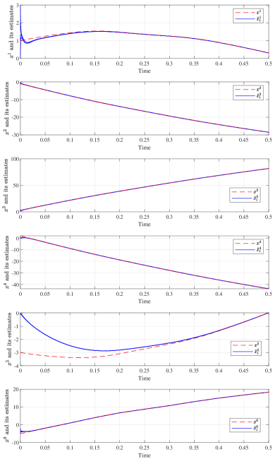
Figure 4: Estimated state vectors along with the state vector of the dynamical system in the presence of unknown inputs for all the nodes in Scenario 1.

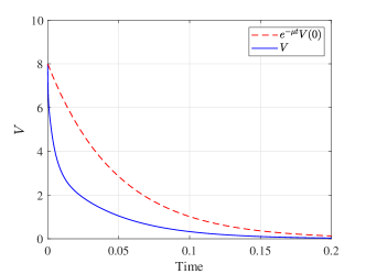
Figure 5: Lyapunov function $V$ generated by the proposed distributed observer in Scenario 1.

Scenario 2 (Directed graph).

In the second scenario, the nodes are assumed to be connected via the unbalanced directed communication graph depicted in Fig. 2b. Distributed state estimation is based on the distributed observers given in (55) where $N_{i}$, $M_{i}$, $L_{i}$, $H_{i}$, and $P_{i}$ still are the same as Scenario 1 as given in Appendix B. According to Lemma 4, $R=\operatorname*{diag}(0.5714,1.714,0.5714,1.143)$, and following (58), $\chi$ is set to $234.0$. Under these conditions, the estimated state vectors of the observers along with the true state vector of the system are illustrated in Fig. 6. According to the figure, the estimated state vectors of all the observers converge to the true state vector of the system asymptotically.

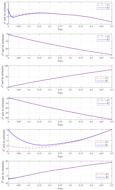
Figure 6: Estimated state vectors along with the state vector of the dynamical system in the presence of unknown inputs for all the nodes in Scenario 2.

Scenario 3 (Switching undirected graph).

In the third scenario, the nodes are assumed to be connected under the switching communication topology depicted in Fig. 3, such that the information exchange starts from Topology 1 and switches to the next topology every $0.1$ second (after Topology 4 the graph switches back to Topology 1). Distributed state estimation is based on the distributed observers given in (52) where $N_{i}$, $M_{i}$, $L_{i}$, $H_{i}$, and $P_{i}$ are the same as Scenario 1 as given in Appendix B. Moreover, $\mathcal{C}(4)$ is calculated as $4.167\times 10^{-2}$, and $\chi$ is set to $4.024\times 10^{3}$ by following (54). Under these conditions, the estimated state vectors of the observers along with true state vector of the system are illustrated in Fig. 7, verifying that the estimated state vectors of all the observers converge to the true state vector of the system asymptotically.

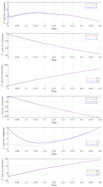
Figure 7: Estimated state vectors along with the state vector of the dynamical system in the presence of unknown inputs for all the nodes in Scenario 3.

6 Conclusions and Future Work

Distributed state estimation of a class of LTI systems was addressed, where the system outputs are measured via a network of sensors distributed within $N$ nodes, and the local measurements at each node are not sufficient for local state estimation. We proposed a DUIO consisting of $N$ local observers co-located with the $N$ nodes and connected via a communication network such that the full state vector of the system is estimated by each local observer. The main motivation for proposing this distributed solution is to account for partial measurements, but more remarkably for inputs that may not be available locally at a node, together with other unknown disturbances. The feasible solution of an LMI provides adequate choices of parameters that guarantee convergence of the estimation errors, under some joint detectability conditions. Furthermore, necessary and sufficient existence conditions are given that are in line with existing theorems for the centralized cases. Finally, we provide modified versions of our main result allowing us to include more complex scenarios in our study, such as switching network topologies and directed communication links. It should be noted that this study was a primary effort on DUIOs, and many problems such as designing DUIOs in the presence of measurement noise as well as expanding the obtained results to discrete-time domains remain open to be studied as future work.

Appendix

Appendix A Derivation of Equation (5)

The equation to be proved is obtained by expanding the error definition (3) along with the system dynamics (1), the output equation (2), and the local observer (4). We start by noting that

$$e_{i}=x-z_{i}-H_{i}y_{i}=(I_{n}-H_{i}C_{i})x-z_{i}.$$ (59)

Taking the time derivative of (59) yields

$$\dot{e}_{i}= (I_{n}-H_{i}C_{i})(Ax+B_{i}u_{i}+\bar{B}_{i}\acute{w}_{i})$$

$$-N_{i}z_{i}-M_{i}B_{i}u_{i}-L_{i}y_{i}-\chi P_{i}^{-1}\sum_{j=1}^{N}a_{ij}(\hat{x}_{j}-\hat{x}_{i}),$$

which by adding and subtracting the term $(I_{n}-H_{i}C_{i})A\hat{x}_{i}$ to the right-hand side and since $\hat{x}_{i}=z_{i}+H_{i}y_{i}$, can be restated as follows:

$$\dot{e}_{i}= (I_{n}-H_{i}C_{i})Ae_{i}+(I_{n}-H_{i}C_{i}-M_{i})B_{i}u_{i}$$ (60)

$$+(I_{n}-H_{i}C_{i})\bar{B}_{i}\acute{w}_{i}+(I_{n}-H_{i}C_{i})A(z_{i}+H_{i}y_{i})$$

$$-N_{i}z_{i}-L_{i}y_{i}-\chi P_{i}^{-1}\sum_{j=1}^{N}a_{ij}(\hat{x}_{j}-\hat{x}_{i}).$$

According to the definition of $e_{i}$, one gets

$$-K_{i}C_{i}e_{i}+K_{i}C_{i}(x-\hat{x}_{i})=\mathbf{0}_{n\times 1}.$$ (61)

Since $\hat{x}_{i}=z_{i}+H_{i}y_{i}$, from (61), it follows that

$$-K_{i}C_{i}e_{i}+K_{i}y_{i}-K_{i}C_{i}z_{i}-K_{i}C_{i}H_{i}y_{i}=\mathbf{0}_{n\times 1}.$$ (62)

We note that

$$\hat{x}_{j}-\hat{x}_{i}=x-\hat{x}_{i}-(x-\hat{x}_{j})=e_{i}-e_{j}.$$ (63)

Now, by adding the zero term (62) to the right hand side of (60) and by considering (63), after grouping similar terms, we finally obtain (5). $\blacksquare$

Appendix B Simulation Parameters in Section V

In this section, we keep $4$ significant digits for noninteger elements in all matrices. The following parameters are used for all three scenarios.

$$F =\begin{bmatrix}7.445&15.70&24.16&11.19&-19.81&8.128\\ 5.254&4.307&8.581&6.864&7.416&-2.586\\ -4.382&-23.23&-33.65&-30.91&-6.951&18.01\end{bmatrix},$$

$$\vskip 3.0pt plus 1.0pt minus 1.0ptP_{1} =P_{2}=P_{3}=P_{4}=0.1000\times I_{6},$$

$$N_{1} =\begin{bmatrix}-205.0&-3.400&8.750&5.000&-16.00&-216.0\\ 0&-214.3&0.4000&0&0&0\\ 0&0.4000&-313.0&0&0&0\\ 546.0&4.667&7.000&-15.00&5.000&555.0\\ 12.40&-2.000&7.800&3.000&-11.00&27.40\\ -647.0&-3.667&-15.33&-5.000&16.00&-636.0\end{bmatrix},$$

$$N_{2} =\begin{bmatrix}2.000&6.000&-5.250&-1.000&8.000&-4.250\\ 2.000&6.000&3.000&-1.000&8.000&4.000\\ -2.000&-6.000&-3.000&1.000&-8.000&-4.000\\ 20.00&-13.00&7.000&-15.00&5.000&7.000\\ -14.20&43.00&0.6005&3.000&-11.00&0.8004\\ 3.667&6.000&4.667&-1.000&8.000&4.000\end{bmatrix},$$

$$N_{3} =\begin{bmatrix}-218.0&-4.400&0&0&0&0\\ -4.400&-214.3&0&0&0&0\\ -8.250&1.400&-8.000&-7.000&-16.00&5.000\\ 212.0&4.667&-15.00&-15.00&5.000&7.000\\ 53.80&-2.000&7.799&3.000&-11.00&0.8002\\ 1093&-3.667&8.000&7.000&16.00&-5.000\end{bmatrix},$$

$$N_{4} =\begin{bmatrix}-216.0&4.200&6.750&-203.0&-5.000&-229.4\\ 0&-214.3&0.4000&0&0&0\\ 0&0.4000&-313.0&0&0&0\\ -579.0&4.667&7.000&-592.0&5.000&-570.0\\ -39.00&-47.00&7.801&-29.00&-11.00&-69.00\\ 0&-2.667&1.667&0&0&0\end{bmatrix}.$$

$$M_{1} =\begin{bmatrix}1&0&0&0&0&0\\ 0&0&0&0&0&0\\ 0&0&0&0&0&0\\ 0&0&0&1&0&0\\ 0&0&0&0&1&0\\ -1&0&0&0&0&0\end{bmatrix},M_{2}=\begin{bmatrix}0&1&0&0&0&0\\ 0&1&0&0&0&0\\ 0&-1&0&0&0&0\\ 0&0&0&1&0&0\\ 0&0&0&0&1&0\\ 0&1&0&0&0&0\end{bmatrix},$$

$$M_{3} =\begin{bmatrix}0&0&0&0&0&0\\ 0&0&0&0&0&0\\ 0&0&1&0&0&0\\ 0&0&0&1&0&0\\ 0&0&0&0&1&0\\ 0&0&-1&0&0&0\end{bmatrix},M_{4}=\begin{bmatrix}0&0&0&-1&0&0\\ 0&0&0&0&0&0\\ 0&0&0&0&0&0\\ 0&0&0&1&0&0\\ 0&0&0&0&1&0\\ 0&0&0&0&0&0\end{bmatrix}.$$

$$L_{1} =\begin{bmatrix}1&17&2\\ 0&0&0\\ 0&0&0\\ -13&-15&7\\ 43&15&8\\ -1&-17&-2\end{bmatrix},L_{2}=\begin{bmatrix}-3&2&4\\ -3&2&4\\ 3&-2&-4\\ -20&-2&7\\ 14&-7&8\\ -3&2&4\end{bmatrix},$$

$$L_{3} =\begin{bmatrix}3.095\times 10^{-3}&0&8.646\times 10^{-4}\\ 6.644\times 10^{-4}&0&8.238\times 10^{-4}\\ -5.001&1.000&4.999\\ -9.002&-13.00&7.000\\ -15.00&43.00&7.999\\ 4.987&-1.000&-5.004\end{bmatrix},$$

$$L_{4} =\begin{bmatrix}2.001&22.00&15.00&-8.999\\ 0&7.377\times 10^{-4}&0&7.435\times 10^{-4}\\ 0&0&0&-2.423\times 10^{-4}\\ -1.996&-22.00&-15.00&9.001\\ -6.999&28.00&15.00&15.00\\ 0&0&0&0\end{bmatrix}.$$

$$H_{1} =\begin{bmatrix}0&0&0\\ 1&0&0\\ 0&1&0\\ 0&0&0\\ 0&0&0\\ 0&0&1\end{bmatrix},H_{2}=\begin{bmatrix}-1&1&0\\ 0&0&0\\ 1&0&0\\ 0&0&0\\ 0&0&0\\ -1&0&1\end{bmatrix},$$

$$H_{3} =\begin{bmatrix}1&0&0\\ 0&1&0\\ 0&0&0\\ 0&0&0\\ 0&0&0\\ -1&0&1\end{bmatrix},H_{4}=\begin{bmatrix}1&1&0&-1\\ 0&1&0&0\\ 0&0&1&0\\ 0&0&0&0\\ 0&0&0&0\\ 0&-1&0&1\end{bmatrix}.$$

References

- [1] R. Casado-Vara, A. Martin-del Rey, S. Affes, J. Prieto, and J. M. Corchado, “IoT network slicing on virtual layers of homogeneous data for improved algorithm operation in smart buildings,” Future Generation Computer Systems, vol. 102, pp. 965–977, 2020.
- [2] M. Bartos, B. Wong, and B. Kerkez, “Open storm: A complete framework for sensing and control of urban watersheds,” Environmental Science: Water Research & Technology, vol. 4, no. 3, pp. 346–358, 2018.
- [3] E. Fadel, V. C. Gungor, L. Nassef, N. Akkari, M. A. Malik, S. Almasri, and I. F. Akyildiz, “A survey on wireless sensor networks for smart grid,” Computer Communications, vol. 71, pp. 22–33, 2015.
- [4] R. Olfati-Saber, “Distributed Kalman filtering for sensor networks,” in Proceedings of the 46th IEEE Conference on Decision and Control, (New Orleans, LA, USA), pp. 5492–5498, December 2007.
- [5] M. Kamgarpour and C. Tomlin, “Convergence properties of a decentralized Kalman filter,” in Proceedings of the 47th IEEE Conference on Decision and Control, (Cancun, Mexico), pp. 3205–3210, December 2008.
- [6] L. Wang and A. S. Morse, “A distributed observer for a time-invariant linear system,” IEEE Transactions on Automatic Control, vol. 63, pp. 2123–2130, July 2018.
- [7] T. Kim, H. Shim, and D. D. Cho, “Distributed Luenberger observer design,” in Proceedings of the 55th IEEE Conference on Decision and Control, (Las Vegas, NV, USA), pp. 6928–6933, December 2016.
- [8] W. Han, H. L. Trentelman, Z. Wang, and Y. Shen, “A simple approach to distributed observer design for linear systems,” IEEE Transactions on Automatic Control, vol. 64, pp. 329–336, January 2019.
- [9] A. Mitra, J. A. Richards, S. Bagchi, and S. Sundaram, “Resilient distributed state estimation with mobile agents: overcoming Byzantine adversaries, communication losses, and intermittent measurements,” Autonomous Robots, vol. 43, pp. 743–768, March 2019.
- [10] A. Mitra and S. Sundaram, “Byzantine-resilient distributed observers for LTI systems,” Automatica, vol. 108, pp. 1–12, October 2019.
- [11] G. Yang, H. Rezaee, and T. Parisini, “Distributed state estimation for a class of jointly observable nonlinear systems,” in Proceedings of the 21st IFAC World Congress, (Berlin, Germany), pp. 5045–5050, July 2020.
- [12] X. He, W. Xue, X. Zhang, and H. Fang, “Distributed filtering for uncertain systems under switching sensor networks and quantized communications,” Automatica, vol. 114, pp. 1–13, April 2020.
- [13] V. Ugrinovskii, “Distributed robust estimation over randomly switching networks using consensus,” Automatica, vol. 49, pp. 160–168, January 2013.
- [14] H. Xu, J. Wang, H. Wang, S. Zhao, and H. Lin, “Distributed observer design for achieving asymptotical omniscience over time-variant disconnected networks,” in Proceedings of the 21st IFAC World Congress, (Berlin, Germany), pp. 3565–3570, July 2020.
- [15] B. Shen, Z. Wang, and Y. S. Hung, “Distributed -consensus filtering in sensor networks with multiple missing measurements: The finite-horizon case,” Automatica, vol. 46, pp. 1682–1688, October 2010.
- [16] M. Farina, G. Ferrari-Trecate, and R. Scattolini, “Distributed moving horizon estimation for linear constrained systems,” IEEE Transactions on Automatic Control, vol. 55, pp. 2462–2475, November 2010.
- [17] W. M. Wonham, Linear Multivariable Control a Geometric Approach. New York, NY, USA: Springer, 3rd ed., 1985.
- [18] W. Ren, R. W. Beard, and E. M. Atkins, “Information consensus in multivehicle cooperative control,” IEEE Control Systems Magazine, vol. 27, pp. 71–82, April 2007.
- [19] R. Olfati-Saber and R. M. Murray, “Consensus problems in networks of agents with switching topology and time-delays,” IEEE Transactions on Automatic Control, vol. 49, pp. 1520–1533, September 2004.
- [20] J. Chen, R. J. Patton, and H.-Y. Zhang, “Design of unknown input observers and robust fault detection filters,” International Journal of control, vol. 63, no. 1, pp. 85–105, 1996.
- [21] M. Darouach, M. Zasadzinski, and S. J. Xu, “Full-order observers for linear systems with unknown inputs,” IEEE Transactions on Automatic Control, vol. 39, pp. 606–609, March 1994.
- [22] S.-H. Wang, E. Wang, and P. Dorato, “Observing the states of systems with unmeasurable disturbances,” IEEE transactions on Automatic Control, vol. 20, pp. 716–717, October 1975.
- [23] Y. Guan and M. Saif, “A novel approach to the design of unknown input observers,” IEEE Transactions on Automatic Control, vol. 36, pp. 632–635, May 1991.
- [24] M. Hou and P. Muller, “Design of observers for linear systems with unknown inputs,” IEEE Transactions on Automatic Control, vol. 37, pp. 871–875, May 1992.
- [25] A. M. Pertew, H. J. Marquez, and Q. Zhao, “Design of unknown input observers for Lipschitz nonlinear systems,” in Proceedings of the American Control Conference, (Portland, OR, USA), pp. 4198–4203, June 2005.
- [26] S. Bhattacharyya, “Observer design for linear systems with unknown inputs,” IEEE transactions on Automatic Control, vol. 23, pp. 483–484, June 1978.
- [27] C. Commault, J. Dion, O. Sename, and R. Motyeian, “Unknown input observer—A structural approach,” in Proceedings of the European Control Conference, (Porto, Portugal), pp. 888–893, September 2001.
- [28] S. P. Boyd, L. E. Ghaoui, E. Feron, and V. Balakrishnan, Linear Matrix Inequalities in System and Control Theory. Philadelphia, PA, USA: SIAM, 1994.
- [29] H. K. Khalil and J. W. Grizzle, Nonlinear Systems. Upper Saddle River, NJ, USA: Prentice Hall, 3rd ed., 2002.
- [30] P. J. Antsaklis and A. N. Michel, Linear Systems. New York, NY, USA: Springer Science & Business Media, 2006.
- [31] M. Pirani and S. Sundaram, “On the smallest eigenvalue of grounded Laplacian matrices,” IEEE Transactions on Automatic Control, vol. 61, pp. 509–514, February 2016.
- [32] F. R. Chung, Spectral Graph Theory. Providence, RI, USA: American Mathematical Society, 1997.
- [33] Z. Li and Z. Duan, Cooperative Control of Multi-Agent Systems: A Consensus Region Approach. Boca Raton, FL: CRC Press, 2017.
- [34] S. Boyd and L. Vandenberghe, Convex Optimization. Cambridge, UK: Cambridge University Press, 2004.