Recurrent Model-Free RL Can Be a Strong Baseline for Many POMDPs
Abstract
Many problems in RL, such as meta-RL, robust RL, generalization in RL, and temporal credit assignment, can be cast as POMDPs. In theory, simply augmenting model-free RL with memory-based architectures, such as recurrent neural networks, provides a general approach to solving all types of POMDPs. However, prior work has found that such recurrent model-free RL methods tend to perform worse than more specialized algorithms that are designed for specific types of POMDPs. This paper revisits this claim. We find that careful architecture and hyperparameter decisions can often yield a recurrent model-free implementation that performs on par with (and occasionally substantially better than) more sophisticated recent techniques. We compare to 21 environments from 6 prior specialized methods and find that our implementation achieves greater sample efficiency and asymptotic performance than these methods on environments. We also release a simple and efficient implementation of recurrent model-free RL for future work to use as a baseline for POMDPs.
1 Introduction

Reinforcement learning (RL) is typically cast as a problem of learning a single fully observable task (an MDP), training and testing on that same task. However, most real-world applications of RL demand some degree of transfer and handling of partial observability. For example, visual navigation (Zhu et al., 2017) requires that robots adapt to unseen scenes with occlusion in observations, and human-robot collaboration requires that robots infer the intentions of human collaborators (Chen et al., 2018).
Many subareas in RL study problems that are special cases of POMDPs (see Table 1). For example, meta-RL (Schmidhuber, 1987; Thrun & Pratt, 2012; Duan et al., 2016; Wang et al., 2017) is a POMDP where certain aspects of the reward function or (less commonly) dynamics function are unobserved but held constant through one episode. The robust RL problem (Bagnell et al., 2001; Rajeswaran et al., 2017a; Pinto et al., 2017; Pattanaik et al., 2018) assumes that certain aspects of the dynamics or reward function are unknown, and aims to find optimal policies that perform well against adversarially-chosen perturbations. Generalization in RL (Whiteson et al., 2011; Zhang et al., 2018a; Packer et al., 2018; Cobbe et al., 2019) focuses on unobserved aspects of the dynamics or reward function that are novel during testing, using an average-case objective instead of the worst-case objective of robust RL. Temporal credit assignment (Sutton, 1984; Arjona-Medina et al., 2019; Hung et al., 2018; Ren et al., 2021) assumes that the reward function is history-dependent and aims to learn to assign credits of current actions to future rewards.
Recent work has proposed efficient and performant algorithms to solve each of these specialized problem settings. However, these algorithms often make assumptions that preclude their application to other POMDPs. For example, methods for robust RL are rarely used for generalization in RL due to objective mismatch (average-case versus worst-case). Similarly, methods for meta-RL are rarely used for temporal credit assignment due to the stationarity assumption in meta-RL.
One method that is applicable to any POMDP is model-free RL equipped with a recurrent policy (actor) and (sometimes) recurrent value function (Duan et al., 2016; Wang et al., 2017; Packer et al., 2018; Igl et al., 2018; Rakelly et al., 2019; Fakoor et al., 2020; Yu et al., 2019). We will refer to this approach as recurrent model-free RL. This baseline is simultaneously simple, as it requires changing only a few lines of code from a model-free RL algorithm, and general, as RNNs (Elman, 1990) are Turing-complete (Siegelmann & Sontag, 1995) and universal function approximators (Schäfer & Zimmermann, 2006).
This approach has been used as a baseline in many prior works, but these prior works report that it performs poorly in many problem settings, including meta-RL (Rakelly et al., 2019; Zintgraf et al., 2020), general POMDPs (Igl et al., 2018; Han et al., 2020), robust RL (Zhang et al., 2021), generalization in RL (Packer et al., 2018), and temporal credit assignment (Arjona-Medina et al., 2019; Raposo et al., 2021). Why does recurrent model-free RL perform poorly? One common explanation is that specialized algorithms or more complicated memory architectures (Ritter et al., 2018; Parisotto et al., 2020) (implicitly) encode inductive biases to solve these specific tasks. For example, algorithms for meta-RL may assume that the underlying dynamics (while unknown) are fixed, and the underlying goals are fixed within one episode (Rakelly et al., 2019; Zintgraf et al., 2020). Similarly, algorithms for robust RL may assume that the dynamics parameters are known (Rajeswaran et al., 2017a) and dynamics is Lipschitz continuous (Jiang et al., 2021). Algorithms for temporal credit assignment sometimes assume that the history-dependent reward can be decomposed into a sum of Markovian rewards (Ren et al., 2021).
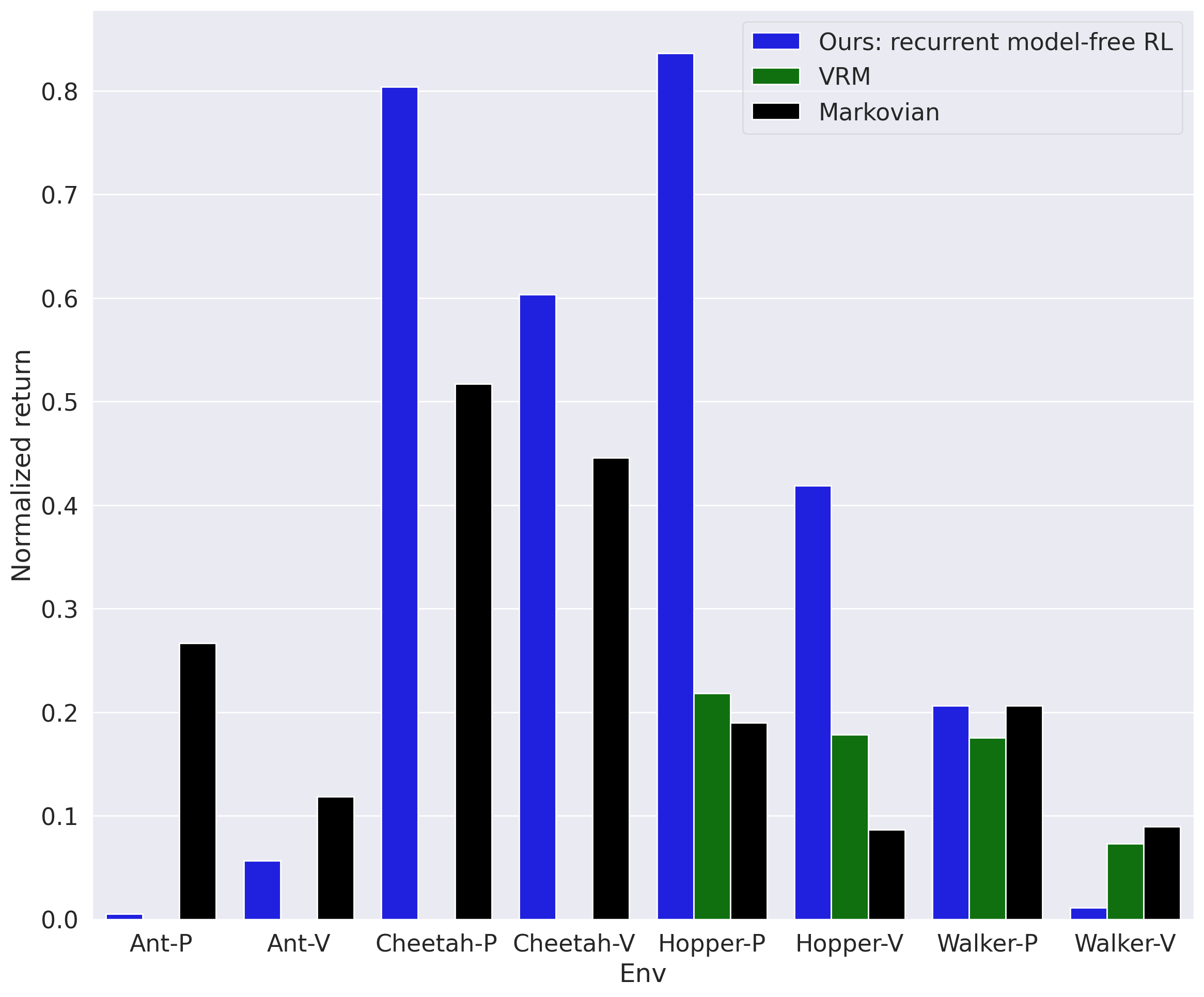
This paper challenges the claim that recurrent model-free RL performs poorly. We argue that, contrary to popular belief, recurrent model-free RL can be competitive with recent state-of-the-art algorithms across a range of different POMDP settings. Similar to the spirit in prior work in Markovian PPO (Engstrom et al., 2020; Andrychowicz et al., 2021) and recurrent DQN (Kapturowski et al., 2019), our experiments show that the implementation of recurrent model-free RL matters. Through extensive experiments (e.g., Fig. 1 shows results on an occluded locomotion benchmark), we show that the careful design and implementation of recurrent model-free RL is critical to its performance. Design decisions such as the actor-critic architecture, the underlying model-free RL algorithm, and context length in RNNs are especially important.
The main contribution of this paper is a performant implementation of recurrent-model free RL. We demonstrate that simple yet important design decisions, such as the underlying RL algorithm and the context length, can often yield a recurrent model-free RL algorithm that performs (at least) on par with prior specialized POMDP algorithms on the benchmarks those algorithms were designed to solve. Ablation experiments identify the importance of these design decisions. We have released the code that is easy to use and memory-efficient.
2 Background
MDP.
A Markov decision process (MDP) (Bellman, 1957) is a tuple , where is the set of states, is the set of actions, is the transition function (dynamics), is the initial state distribution, is the reward function, is the time horizon, and is the discount factor. Solving an MDP requires learning a policy that maximizes the expected discounted return: . For any MDP, there exists an optimal policy that is memoryless (Puterman, 2014). MaxEnt RL algorithms (Ziebart, 2010; Haarnoja et al., 2018a) add an entropy bonus to the RL objective.
POMDP.
A partially observable Markov decision process (POMDP) (Åström, 1965) is a tuple , where the underlying process is an MDP . Let be the set of observations and let be the emission function. Let the observable trajectory up to time-step be , the memory-based policy in the most general form is defined as , conditioning on the whole history. At the first time step , an initial state and an initial observation are sampled. At any time-step , the policy emits the action to the system, the system updates the state following the dynamics, , the next observation is sampled and the reward is computed as .
We refer to the part of the state at current time-step that can be directly unveiled from current observation as the observable state , and the rest part of the state as the hidden state . We call the hidden state stationary if it does not change within an episode. The average-case and worst-case objectives for POMDPs can be written as:
| (average-case) | |||
| (worst-case) |
3 Related Work
| Subarea | in dynamics? | in reward? | Is stationary? | Agent input | RL objective | Domain shift? |
| “Standard” POMDP | ✓ | ✓ | ✗ | oar | Avg | ✗ |
| Meta-RL | ✗* | ✓ | ✓ | oard | Avg | ✗ |
| Robust RL | ✓* | ✗* | ✓* | oa | Worst | ✗ |
| Generalization in RL | ✓* | ✗* | ✓* | oa | Avg | ✓* |
| Temporal credit assignment | ✗ | ✓ | ✗ | oa | Avg | ✗ |
We discuss subareas of RL that explicitly or implicitly solve POMDPs, as well as algorithms proposed for these specialized settings. Table 1 summarizes these subareas.
RL for “standard” POMDPs.
We use the term “standard” to refer to prior work that explicitly labels the problems studied as POMDPs. Common tasks include scenarios where the states are partially occluded (Heess et al., 2015), different states correspond to the same observation (perceptual aliasing (Whitehead & Ballard, 1990)), random frames are dropped (Hausknecht & Stone, 2015), observations use egocentric images (Zhu et al., 2017), or the observations are perturbed with random noise (Meng et al., 2021). These POMDPs often have hidden states that are non-stationary and affect both the rewards and the dynamics. POMDPs are hard to solve because of the curse of dimensionality: the size of the history grows linearly with the horizon length (Papadimitriou & Tsitsiklis, 1987; Littman, 1996). Prior POMDP algorithms (Cassandra et al., 1994) attempt to infer the state from the past sequence of observations, and then apply standard RL techniques to that inferred state. Such an inferred state is known as a belief state (Kaelbling et al., 1998). However, exact inference requires the knowledge of the dynamics, emission probabilities, and reward functions, and is intractable in all except the most simple settings. One strategy for solving these general POMDPs is to use memory-based policies, which take the entire history of past observations as inputs. Among the memory architectures, RNNs have been widely used to equip RL algorithms (Schmidhuber, 1991; Bakker, 2001; Wierstra et al., 2007), as they have a simpler design without losing the expressivity (Schäfer & Zimmermann, 2006), compared to more complicated ones, e.g. external memory (Graves et al., 2016; Oh et al., 2016) and episodic memory (Fortunato et al., 2019; Zhu et al., 2020). These recurrent RL strategies can be further subdivided into model-free methods (Heess et al., 2015; Hausknecht & Stone, 2015; Mirowski et al., 2017; Meng et al., 2021), where the single objective is to maximize the return, and model-based methods (Watter et al., 2015; Ha & Schmidhuber, 2018; Igl et al., 2018; Zhang et al., 2018c; Espeholt et al., 2018; Gregor et al., 2019; Hafner et al., 2019; Han et al., 2020; Lee et al., 2020a).that have explicitly inferred the belief state and pass it as an additional input to a memoryless policy. The recurrent model-free RL that we focus on belongs to the class of model-free, off-policy, memory-based algorithms.
Meta-RL.
Meta-RL, also called “learning to learn” (Schmidhuber, 1987; Thrun & Pratt, 2012), focuses on POMDPs where some parameters in the rewards or (less commonly) dynamics are varied from episode to episode, but remain fixed within a single episode (Humplik et al., 2019). These different values of these parameters represent different tasks. The meta-RL setting is almost the same as multi-task RL (Wilson et al., 2007; Yu et al., 2019), but differs in that multi-task RL can observe the task parameters, making it an MDP instead of a POMDP. Algorithms for meta-RL can be roughly categorized based on how the adaptation step is performed. Gradient-based algorithms (Hochreiter et al., 2001; Finn et al., 2017; Fakoor et al., 2020) perform adaptation by running a few gradient steps on the pre-trained models. Memory or context-based algorithms use memory architectures to implicitly adapt. These memory-based methods which can be further subdivided into implicit and explicit task inference methods. Implicit task inference methods (Wang et al., 2017; Duan et al., 2016; Ritter et al., 2018; Espeholt et al., 2018; Parisotto et al., 2020) use an RL objective only to learn memory-based policies. Explicit task inference methods (Zintgraf et al., 2020; Rakelly et al., 2019) train an extra inference model to estimate task embeddings (i.e., a representation of the unobserved parameters) by approximate inference. Task embeddings are then used as additional inputs to memoryless policies.
Robust RL.
The goal of robust RL is to find a policy that maximizes returns in the worst-case environments. Prior work designs deep RL algorithms that are robust against perturbations to the dynamics (Khalil et al., 1996; Bagnell et al., 2001; Nilim & Ghaoui, 2005; Morimoto & Doya, 2005; Derman et al., 2018; Rajeswaran et al., 2017a; Mankowitz et al., 2020; Jiang et al., 2021), observations (Lin et al., 2017; Pattanaik et al., 2018; Huang et al., 2017; Wang et al., 2019), and actions (Pinto et al., 2017; Gleave et al., 2020; Tessler et al., 2019). Treating the robust RL problem as a POMDP, rather than an MDP (as done in most prior work), unlocks a key capability: using memory to identify the hidden state within a single episode. While some work find memory-based policies are more robust to adversarial attacks than Markovian policies (Russo & Proutière, 2021; Zhang et al., 2021), they train these baselines in a single MDP without adversaries. In contrast, we will train recurrent model-free RL on a distribution of MDPs.
Generalization in RL.
The goal of generalization in RL is to make RL algorithms perform well in test domains that are unseen during training. This setting differs from robust RL because it uses an average-case objective instead of a worst-case objective. In this sense, meta-RL is closely related to (in-distribution) generalization in RL. Prior work has studied generalization to initial states in the same MDP (Whiteson et al., 2011; Rajeswaran et al., 2017b; Zhang et al., 2018b), to random disturbance in dynamics (Rajeswaran et al., 2017b), states (Stulp et al., 2011), observations (Zhang et al., 2018a; Song et al., 2020), and actions (Srouji et al., 2018), and to different modes in procedurally generated games (Justesen et al., 2018; Farebrother et al., 2018; Cobbe et al., 2019). Among them, Packer et al. (2018); Zhao et al. (2019) provide benchmarks on both in-distribution and out-of-distribution generalization to different dynamics parameters. Algorithms for improving generalization in RL can be roughly divided into regularization-based methods (Farebrother et al., 2018; Cobbe et al., 2020; Igl et al., 2019), methods that use special model architectures (Srouji et al., 2018; Raileanu & Fergus, 2021), and methods that use data augmentation (Tobin et al., 2017; Lee et al., 2020b). While randomizing the dynamics or observations implicitly transforms an MDP into a POMDP, these prior methods normally use memoryless RL algorithms. By contrast, we consider memory-based RL algorithms that can adapt online for generalization (Kirk et al., 2021, Sec. 5.2).
Temporal credit assignment.
POMDPs are sometimes disguised as MDPs. For example, delaying the reward signals (Sutton, 1984; Arjona-Medina et al., 2019) can make an MDP into a POMDP, as the rewards at current time still depend on previous observations and/or actions, given current observations. Similarly, when rewards are defined in terms of trajectories (Liu et al., 2019; Ren et al., 2021) (episodic rewards), the problem can likewise become a POMDP. Algorithms to solve these problems belong to temporal credit assignment subarea (Hung et al., 2018). While prior work has applies recurrent model-free RL to these problem settings, it has been reported with poor performance (Hung et al., 2018; Liu et al., 2019; Arjona-Medina et al., 2019; Raposo et al., 2021). Methods to tackle delayed rewards include stacking recent observations to make the problems as MDPs (Katsikopoulos & Engelbrecht, 2003), tuning the discount factor (Fedus et al., 2019) and lambda in eligibility traces (Xu et al., 2020) to increase effective horizons, and using hindsight and counterfactuals to reduce the variance of policy gradients (Harutyunyan et al., 2019; Mesnard et al., 2021). A popular branch of specialized methods, is to learn surrogate reward functions for efficient learning, e.g. return decomposition into a sum of (dense) rewards (Liu et al., 2019; Ren et al., 2021; Raposo et al., 2021), and reward redistribution across time (Hung et al., 2018; Arjona-Medina et al., 2019; Ferret et al., 2020; Gangwani et al., 2020).
4 Design Considerations for Recurrent Model-Free RL
Implementing a recurrent model-free RL algorithm requires making a number of design decisions. In the following paragraphs, we will describe the important decision factors we find in recurrent model-free RL. Table 2 summarizes how prior work and our work make these design decisions.
| Algorithm | Domain / Benchmark | Arch | Encoder | Inputs | Len | RL |
| Duan et al. (2016) | Meta-RL | separate | GRU | oard | 1000 | TRPO, PPO |
| Wang et al. (2017) | Meta-RL | shared | LSTM | oart | 5-150 | A2C |
| Baseline in Rakelly et al. (2019) | Meta-RL | separate | GRU | oard | 100 | PPO |
| Baseline in Zintgraf et al. (2020) | Meta-RL | separate | GRU | oard | Max | A2C, PPO |
| Baseline in Fakoor et al. (2020) | Meta-RL | separate | GRU | oar | 10-25 | TD3 |
| Baseline in Yu et al. (2019) | Meta-RL | separate | GRU | oard | 500 | PPO |
| Kostrikov (2018) | POMDP | shared | GRU | o | 5-2048 | PPO, A2C |
| Ding (2019) | POMDP | separate | LSTM | oa | 150 | TD3, SAC |
| Meng et al. (2021) | POMDP | separate | LSTM | oa | 1-5 | TD3 |
| Yang & Nguyen (2021) | POMDP | separate | both | oa | Max | TD3, SAC |
| Baseline in Igl et al. (2018) | POMDP | shared | GRU | oa | 25 | A2C |
| Baseline in Han et al. (2020) | POMDP | shared | LSTM | o | 64 | SAC |
| Baseline in Zhang et al. (2021) | Robust RL | separate | LSTM | o | 100 | PPO |
| Baseline 1 in Packer et al. (2018) | Generalization in RL | shared | LSTM | o | 128-512 | PPO, A2C |
| Baseline 2 in Packer et al. (2018) | Generalization in RL | separate | LSTM | oard | 128-512 | PPO, A2C |
| Baseline in Hung et al. (2018) | Temporal credit assignment | shared | LSTM | oar | Max | A3C |
| Baseline in Liu et al. (2019) | Temporal credit assignment | separate | LSTM | oa | Max | PPO |
| Baseline in Raposo et al. (2021) | Temporal credit assignment | shared | LSTM | oar | 10-60 | IMPALA |
| Our work | Meta-RL (Dorfman et al., 2020) | separate | LSTM | oard | 64 | TD3 |
| Meta-RL (Zintgraf et al., 2020) | separate | GRU | oard | Max | SAC | |
| POMDP (Han et al., 2020) | separate | GRU | oa | 64 | TD3 | |
| Robust RL (Jiang et al., 2021) | separate | LSTM | o | 64 | TD3 | |
| Generalization in RL (Packer et al., 2018) | separate | LSTM | o | 64 | TD3 | |
| Temporal credit assignment (Raposo et al., 2021) | separate | LSTM | o | Max | SAC-D |
Recurrent (off-policy) actor-critic architecture.
The first important design decision is whether the recurrent policy (actor) and the recurrent Q-value function (critic) use a shared RNN encoder (and embedders) or use separate ones. In our experiments (Sec. 5.2), we show that a shared encoder increases the gradient norm and hinders learning. While recent work has adopted the design of separate encoders (Fakoor et al., 2020; Ding, 2019; Meng et al., 2021; Sun et al., 2021; Weng et al., 2021), some implementations of recurrent model-free RL use the (inferior) shared encoder. After running some experiments to compare this design decision, we will use the separate architecture in the rest of the paper.
Agent inputs.
The next consideration is the choice of inputs for the actor and critic. While prior work often only conditions the recurrent RL baseline on previous observations (and actions) (Igl et al., 2018; Kostrikov, 2018; Han et al., 2020; Ding, 2019; Meng et al., 2021; Yang & Nguyen, 2021), our experiments in Sec. 5.2 find that additionally conditioning on other previous information, such as previous rewards, can increase return by up to . Table 1 shows which inputs we found useful for which types of POMDPs.
Model-free RL algorithm.
Recurrent model-free RL can be understood as applying an off-the-shelf model-free RL algorithm with an actor and a Q function conditioned on sequences of inputs. As such, the choice of the underlying model-free RL algorithm is paramount. in While off-policy algorithms such as TD3 (Fujimoto et al., 2018) and SAC (Haarnoja et al., 2018a, b) improve sample efficiency and asymptotic performance in continuous control tasks, these RL algorithms are rarely used in recurrent model-free RL baselines (Rakelly et al., 2019; Zintgraf et al., 2020; Zhang et al., 2020). Our experiments show that using these off-policy algorithms for recurrent model-free RL generally works better than recurrent model-free RL implementations that use on-policy algorithms. This result echoes the finding that model-free off-policy TD3-Context (Fakoor et al., 2020) can be better than the specialized method PEARL (Rakelly et al., 2019) in meta-RL.
RNN variants and context length.
RNN training is known to be unstable, especially with long sequences input (Bengio et al., 1994). RNN variants like LSTM (Hochreiter & Schmidhuber, 1997) and GRU (Chung et al., 2014) can mitigate the training issues, but still may fail to learn long-term dependencies (Trinh et al., 2018). We study two design decisions here: the RNN architecture (LSTM, GRU) and the context length, i.e. the length of sequence fed into RNN for training. We find that the architecture has a minor effect on the final performance (App. E.2). Prior POMDP methods use context lengths ranging from 1 to 2048 (see the “Len” column of Table 2), and we select three representatives of short (5), medium (64), and long length (larger than 100) in the experiments for comparison. We find that the optimal context length is task-specific (Sec. 5.2). For example, a POMDP that hides velocities from observations theoretically only requires a short context length to infer velocities through consecutive positions (Meng et al., 2021).



5 Experiments
Our experiments aim to answer two questions. First, how does a well-tuned implementation of recurrent model-free RL compare to specialized POMDP methods? To give these prior methods the strongest possible footing, we perform the comparison on the benchmarks used by these prior methods. Second, which design decisions are essential for recurrent model-free RL? We put the environment details in App. D.
Code implementation.
We release a modular and configurable implementation of recurrent (off-policy) model-free RL in the supplementary material. Our implementation is efficient in terms of computer memory compared to previous off-policy RL methods for POMDPs. For example, our implementation uses 200x less RAM than Han et al. (2020) and 9x less GPU memory than Dorfman et al. (2020).
5.1 Recurrent Model-Free RL is Comparable with Prior Specialized Methods on Their Benchmarks
Recurrent model-free RL is a ubiquitous baseline across a range of different POMDP settings (e.g., meta-RL, occluded observations, delayed rewards) (Rakelly et al., 2019; Zintgraf et al., 2020; Humplik et al., 2019; Igl et al., 2018; Han et al., 2020; Arjona-Medina et al., 2019). This section casts doubt on that claim, showing that a well-tuned implementation of recurrent model-free RL can perform at least as well as more complex or specialized methods in most of their experimented environments.
We tune a wide range of decision factors, shown in Sec. 4. App. A.3 shows the detailed options of each decision factor. For each subarea, we select one recent specialized method and use the same benchmark as used in the paper proposing that method. For meta-RL, we perform one additional comparison.
For each benchmark, we show the performance of a single variant among our design combinations that works best across the environments in that benchmark; in other words, we use the same hyperparameters for each task within a benchmark, and do not tune hyperparameters individually for each task. The exact configurations of each benchmark can be found in the last five rows of Table 2. Our implementation is at least comparable to (and sometimes outperforms by a wide margin) prior specialized methods across most tasks (18 out of 21 environments). Our method performs especially well in terms of sample efficiency. However, we find one benchmark where it performs worse on 2 out of 3 environments (Ant-Dir and Humanoid-Dir from on-policy variBAD (Zintgraf et al., 2020)). This result is not entirely surprising, as on-policy methods typically outperform off-policy methods (which our implementation uses) on the fully-observed versions of these tasks (see Fig. 12).
For each plot of learning curves, we show three approaches as references. First, an oracle policy has access to the POMDP hidden states, turning the POMDP into an MDP. This policy should therefore be treated as an upper bound on the performance that any POMDP method should receive. Second, as a lower bound, we use a Markovian policy to solve the POMDP. Both oracle policy and Markovian policy are trained with the same hyperparameters as our recurrent model-free RL implementation. We also compare to a random policy, which represents a trivial lower bound. We show the complete learning curves in App. E.1 and numerical results in Table 7, and provide implementation details in App. B.
“Standard” POMDP.
We study “standard” POMDPs by looking at tasks that typically occlude some part of the observation. We will compare against VRM (Han et al., 2020), a recent, state-of-the-art, model-based POMDP algorithm. We adopt the occlusion benchmark proposed by VRM and there are 8 environments Hopper, Ant, Walker, Cheetah-P, V, where “-P” stands for observing positions and angles only, and “-V” stands for observing velocities only.
Fig. 1 and Fig. 22 show that the best single variant of our model-free recurrent RL implementation outperforms VRM in 6 out of 8 environments, especially in Cheetah, Hopper-P (over of the oracles). Our results suggest that, while the variational dynamics model used by VRM may be useful for some tasks, this model is not necessary to achieve high results. While we are primarily interested in sample complexity, but not compute, it is worth noting that our recurrent model-free RL implementation is substantially more efficient than the open-source VRM implementation: our implementation trains faster and can reduce RAM usage (see App. A).
Meta-RL.
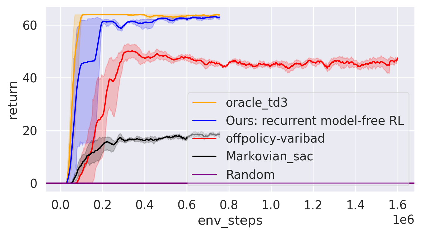
We next study the meta-RL setting, where some indicator of the task is unobserved. We compare our implementation of recurrent model-free RL to a specialized, state-of-the-art method, variBAD (Zintgraf et al., 2020). VariBAD explicitly learns task embeddings using a variational, model-based objective. While the variBAD was originally proposed using PPO (Zintgraf et al., 2020), recent work has effectively used the same method with SAC (Dorfman et al., 2020). We refer to these methods as on-policy variBAD and off-policy variBAD, and will compare to both of them. Importantly, we use the same environments as the papers that proposed these methods. The environments proposed for off-policy variBAD are relatively easy: Semi-Circle, Wind, and Cheetah-Vel. We adapt Wind to make it harder to solve. Off-policy variBAD is shown to have superior performance over on-policy variBAD in this benchmark (Dorfman et al., 2020, Fig. 11). The environments proposed for on-policy one are harder: Ant, Cheetah, Humanoid-Dir. On-policy variBAD outperforms RL2 (Duan et al., 2016) in this benchmark (Zintgraf et al., 2021, Fig. 13).
Fig. 2 shows that our best single variant outperforms off-policy variBAD on their environments (Semi-Circle and Wind), and on-policy variBAD on their environment (Cheetah-Dir), both in terms of sample efficiency and asymptotic return. While methods like variBAD disentangle task inference from control, potentially stabilizing training, our experiments suggest that stable training might be achieved with simple recurrent model-free RL. As our implementation is off-policy, it has the potential to have better sample efficiency than on-policy variBAD. As our implementation is trained end-to-end, without using pre-trained task representations like off-policy variBAD, it does not have the staleness issue in task representations (Kapturowski et al., 2019). We believe that these factors may contribute to the relatively good performance of recurrent model-free RL. Nevertheless, our implementation performs worse than on-policy variBAD on Ant-Dir (Fig. 2) and Humanoid-Dir (Fig. 12). These negative results are not entirely surprising, as off-policy methods tend to perform worse than on-policy methods on the fully-observed versions of these tasks (compare oracle SAC/TD3 to oracle PPO in Fig. 12).

Robust RL.
We then study robust RL. We choose the recent, specialized algorithm MRPO (Jiang et al., 2021), and adopt their benchmark based on SunBlaze benchmark (Packer et al., 2018). These environments have hidden states that are fixed during one episode, namely Cheetah, Hopper, Walker-Robust. The hidden state includes the density and the friction coefficients of the simulated robots.
Fig. 3 shows both the average return and worst return of our single best variant and MRPO on one environment. Following prior work (Jiang et al., 2021), we measure the worst return using the average return in the worst testing tasks. Despite using the average-case objective, our method achieves better worst-case performance than MRPO, which directly optimizes this worst-case objective. Surprisingly, our method even outperforms the oracle, which has access to hidden state information. Our method is also over 80% more sample-efficient than these alternative approaches. Our limitation of recurrent model-free RL is its slow wall-clock time; our implementation is 17.5x slower than MRPO, given the same simulation steps (see App. A). Nonetheless, we believe that sample efficiency is often a more important factor than computing efficiency.

Generalization in RL.
We study generalization in RL using two environments from the SunBlaze benchmark: Hopper, Cheetah-Generalize. Following the evaluation metrics (Packer et al., 2018, Sec. 6), we report the average success rates in interpolation setting (training and testing on the same POMDP) and extrapolation setting (training on a POMDP with a hidden state distribution of small support, and testing on another POMDP with a hidden state distribution of a disjoint support). We pick the best specialized method in the tables of final performance (Packer et al., 2018, Table 7,8), a Markovian on-policy robust RL method EPOpt-PPO-FF (Rajeswaran et al., 2017a).
Fig. 4 shows interpolation and extrapolation results on one environment. In the interpolation setting, our method performs on par with the best prior method, EPOpt-PPO-FF. In the more challenging extrapolation setting, our method outperforms it and is comparable to the oracle. However, unlike EPOpt-PPO-FF and oracle, our method does not require access to the dynamics parameters.
| Delayed-Catch | Key-to-Door |
Temporal credit assignment.
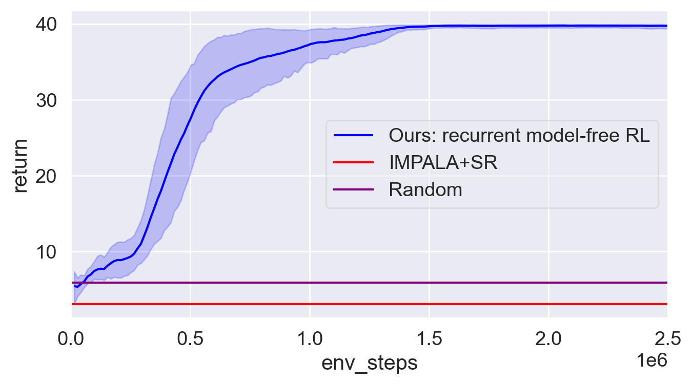
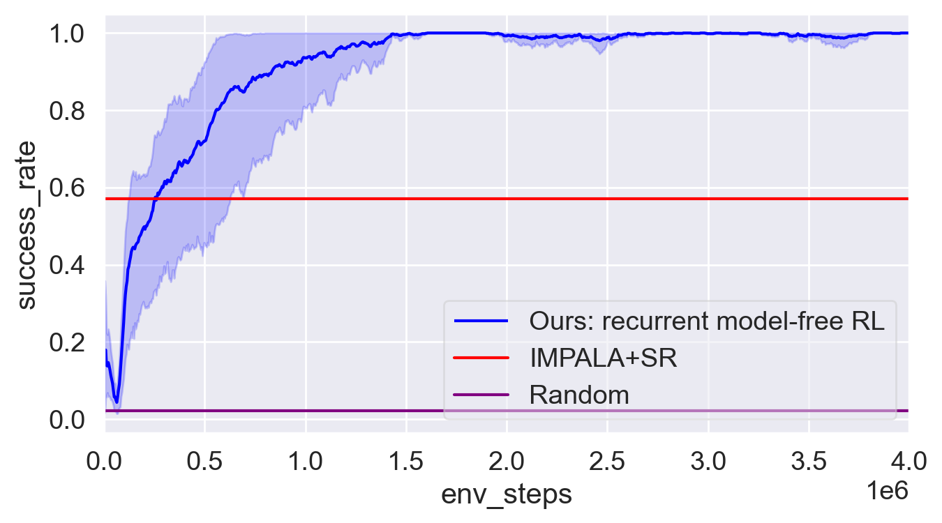
Finally we move on to temporal credit assignment. We choose the recent, specialized algorithm IMPALA+SR (Raposo et al., 2021), and adopt their environments, namely, Delayed-Catch and Key-to-Door. Both tasks have sparse rewards that depend on the whole trajectory, thus the optimal value function should be memory-based, and we did not compare Markovian RL methods. As both tasks are discrete control with pixel input, we adapt the observation embedder into a simple CNN, and select SAC-Discrete (Christodoulou, 2019) as the RL algorithm, which is the discrete version of SAC. We follow IMPALA+SR to use LSTM as encoder and set context length as full episode length. We tune the entropy temperature of SAC-Discrete and find that works well on both tasks.
Discussion on the performance of oracle policies.
One seemingly surprising result is that the oracle policies often underperform our implementation of recurrent model-free RL. We believe that this result is caused by using the same hyperparameters for the oracle policies as for our recurrent model-free implementation. We expect that further tuning of the hyperparameters for the oracle policies would allow them to surpass all the alternative approaches.
In summary, recurrent model-free RL can perform at least as well as more specialized or complex methods on most of their tasks, provided that the implementation is well tuned. The good performance of this baseline across a wide range of tasks and problem types bodes well for its performance on other problems.
5.2 What Matters in Recurrent Model-Free RL Algorithms?
To study what factors explain the good performance of recurrent model-free RL, we will ablate the five important design decisions introduced in Sec. 4: the actor-critic architecture (Arch), the agent input space (Inputs), the underlying model-free RL algorithm (RL), the RNN encoder (Encoder), and the RNN context length (Len). See Table 2 for a summary of how prior work made these design decisions. Due to the space limit, we show the “single factor analysis” plots for each decision factor by averaging the performance over the other factors in App. E.2.

Recurrent off-policy actor-critic architecture.
We study the choice of shared/separated architectures in two simple POMDP environments. The results, shown in Fig. 6 and App. E.3, show that the shared architecture failed to learn either of these tasks. The different scale of RNN gradient norms w.r.t. actor and critic in the shared architecture suggests that the gradient of critic loss may dominate the actor’s. Our results echo prior work (Fakoor et al., 2020; Meng et al., 2021; Sun et al., 2021) that use separate RNN encoders and achieve high asymptotic rewards, and also echo that (Han et al., 2020) shows poor results in the shared architecture of SAC-LSTM.
| Change in one decision factor | Subarea / Benchmark | Environment | Performance comparison |
|---|---|---|---|
| Inputs: oa oar | “Standard” POMDP | Walker-P | 981.6 1345.0 () |
| RL: TD3 SAC | “Standard” POMDP | Ant-P | 310.7 2123.5 () |
| Encoder: LSTM GRU | Robust RL | Walker-Robust | 765.9 931.3 () |
| Len: 64 400 | Meta-RL | Cheetah-Vel | -85.2 -74.6 (+14%) |
| Len: 64 5 | Generalization | Hopper-Generalize | 0.292 0.415 () |
| Len: 64 5 | “Standard” POMDP | Walker-V | 121.4 264.3 () |
Agent inputs.
We next study the choice of agent inputs using the Walker-P task. As shown in Table 3 (row 1), additionally conditioning the agent on past rewards increases performance by . The reward signals could help reveal the missing information of the velocity of the robot base, which is occluded in Walker-P. On other tasks where velocity is occluded, we similarly find that conditioning on past rewards improves performance (see o vs. or in Fig. 16).
Model-free RL algorithms.
Table 2 shows that recurrent model-free RL implementations using TD3 dominate in 4 out of 5 benchmarks. This finding might be partially explained by the fact that most environments have relatively easy dynamics. However, on environments with harder dynamics such as Ant and Humanoid, SAC performs better than TD3. For instance, the 2nd row of Table 3 shows the effect of RL algorithm in a POMDP environment Ant-P. SAC is significantly better than TD3 (increase by 6.8, surpassing the PPO-GRU (Kostrikov, 2018) in Fig. 1). Two exceptions to this rule are Walker-V (Fig. 17) and Ant-Dir (Fig. 2) where on-policy algorithms (PPO-GRU and RL2) outperform off-policy ones as used in our implementation.
RNN variants and context length.
Generally, there is no significant difference between LSTM and GRU (see the single factor analysis in App. E.2). However, the 3rd row of Table 3 shows the effect of RNN encoder in a robust RL environment. We can see replacing LSTM with GRU can increase the worst-case metric in Walker-Robust. For the context length in RNNs, a medium length (64) dominates in all the best variants in most benchmarks (see Table 2), which could be viewed as a trade-off between memory capacity and computation costs. However, the remaining rows of Table 3 show the mixed effects of context length in RNNs. Both increasing and decreasing the context length can boost the performance in different environments. Specifically, decreasing the length from 64 to 5 makes our implementation surpass VRM in Walker-V (increase by 2.2). This result might explain why the prior methods adopt a wide range of context lengths from 1 to 2048 (see Table 2). Therefore, the choice of context length seems to be problem-specific and may require tuning.
Summary.
We now summarize the main findings of our experiments based on the benchmarks:
- 1.
- 2.
- 3.
- 4.
These findings may provide a useful initialization for researchers to study recurrent model-free RL.
6 Conclusion and Future Work
This paper shows that a carefully-designed implementation of recurrent model-free RL can perform well across a range of benchmarks corresponding to different types of POMDPs. In most cases, our implementation performs on par with (if not significantly better than) prior methods that are specifically designed for the corresponding types of POMDPs. Our ablation experiments demonstrate the importance of key design decisions, such as the underlying RL algorithm and the RNN context length. While the best choices for some decisions (such as using separate RNNs for the actor and the critic) seem to be consistent across domains, the best choices for other decisions (such as RNN context length) are problem-dependent. We encourage future work to study automated mechanisms for selecting these crucial design decisions. In releasing our code, we hope to aid future research into the design of stronger POMDP algorithms.
Acknowledgement
We thank Pierre-Luc Bacon, Murtaza Dalal, Paul Pu Liang, Sergey Levine, Evgenii Nikishin, Hao Sun, and Maxime Wabartha for their constructive feedback on the draft of this paper. TN thanks Pierre-Luc Bacon for suggesting temporal credit assignment experiments and Michel Ma and Pierluca D’Oro for their help on the environments. We thank Luisa Zintgraf for sharing the learning curves of on-policy variBAD. TN thanks CMU cluster and Mila cluster for compute resources. This work is supported by the Facebook CIFAR AI Chair, the Fannie and John Hertz Foundation and NSF GRFP (DGE1745016).
References
- Andrychowicz et al. (2021) Andrychowicz, M., Raichuk, A., Stanczyk, P., Orsini, M., Girgin, S., Marinier, R., Hussenot, L., Geist, M., Pietquin, O., Michalski, M., Gelly, S., and Bachem, O. What matters for on-policy deep actor-critic methods? A large-scale study. In 9th International Conference on Learning Representations, ICLR 2021, Virtual Event, Austria, May 3-7, 2021, 2021.
- Arjona-Medina et al. (2019) Arjona-Medina, J. A., Gillhofer, M., Widrich, M., Unterthiner, T., Brandstetter, J., and Hochreiter, S. RUDDER: return decomposition for delayed rewards. In Advances in Neural Information Processing Systems 32: Annual Conference on Neural Information Processing Systems 2019, NeurIPS 2019, December 8-14, 2019, Vancouver, BC, Canada, 2019.
- Åström (1965) Åström, K. J. Optimal control of Markov processes with incomplete state information i. Journal of Mathematical Analysis and Applications, 10:174–205, 1965.
- Bagnell et al. (2001) Bagnell, J. A., Ng, A. Y., and Schneider, J. G. Solving uncertain Markov decision processes. 2001.
- Bakker (2001) Bakker, B. Reinforcement learning with long short-term memory. In Advances in Neural Information Processing Systems 14 [Neural Information Processing Systems: Natural and Synthetic, NIPS 2001, December 3-8, 2001, Vancouver, British Columbia, Canada], 2001.
- Bellman (1957) Bellman, R. A Markovian decision process. Journal of mathematics and mechanics, 6(5):679–684, 1957.
- Bengio et al. (1994) Bengio, Y., Simard, P. Y., and Frasconi, P. Learning long-term dependencies with gradient descent is difficult. IEEE Trans. Neural Networks, 1994.
- Cassandra et al. (1994) Cassandra, A. R., Kaelbling, L. P., and Littman, M. L. Acting optimally in partially observable stochastic domains. In Proceedings of the 12th National Conference on Artificial Intelligence, Seattle, WA, USA, July 31 - August 4, 1994, Volume 2, 1994.
- Chen et al. (2018) Chen, M., Nikolaidis, S., Soh, H., Hsu, D., and Srinivasa, S. S. Planning with trust for human-robot collaboration. In Proceedings of the 2018 ACM/IEEE International Conference on Human-Robot Interaction, HRI 2018, Chicago, IL, USA, March 05-08, 2018, 2018.
- Cho et al. (2014) Cho, K., van Merrienboer, B., Gülçehre, Ç., Bahdanau, D., Bougares, F., Schwenk, H., and Bengio, Y. Learning phrase representations using RNN encoder-decoder for statistical machine translation. In Proceedings of the 2014 Conference on Empirical Methods in Natural Language Processing, EMNLP 2014, October 25-29, 2014, Doha, Qatar, A meeting of SIGDAT, a Special Interest Group of the ACL, 2014.
- Christodoulou (2019) Christodoulou, P. Soft actor-critic for discrete action settings. arXiv preprint arXiv:1910.07207, 2019.
- Chung et al. (2014) Chung, J., Gülçehre, Ç., Cho, K., and Bengio, Y. Empirical evaluation of gated recurrent neural networks on sequence modeling. arXiv preprint arXiv:1412.3555, 2014.
- Cobbe et al. (2019) Cobbe, K., Klimov, O., Hesse, C., Kim, T., and Schulman, J. Quantifying generalization in reinforcement learning. In Proceedings of the 36th International Conference on Machine Learning, ICML 2019, 9-15 June 2019, Long Beach, California, USA, 2019.
- Cobbe et al. (2020) Cobbe, K., Hesse, C., Hilton, J., and Schulman, J. Leveraging procedural generation to benchmark reinforcement learning. In Proceedings of the 37th International Conference on Machine Learning, ICML 2020, 13-18 July 2020, Virtual Event, 2020.
- Coumans & Bai (2016) Coumans, E. and Bai, Y. PyBullet, a python module for physics simulation for games, robotics and machine learning. 2016.
- Derman et al. (2018) Derman, E., Mankowitz, D. J., Mann, T. A., and Mannor, S. Soft-robust actor-critic policy-gradient. In Proceedings of the Thirty-Fourth Conference on Uncertainty in Artificial Intelligence, UAI 2018, Monterey, California, USA, August 6-10, 2018, 2018.
- Ding (2019) Ding, Z. Popular-rl-algorithms. https://github.com/quantumiracle/Popular-RL-Algorithms, 2019.
- Dorfman et al. (2020) Dorfman, R., Shenfeld, I., and Tamar, A. Offline meta learning of exploration. arXiv preprint arXiv:2008.02598, 2020.
- Duan et al. (2016) Duan, Y., Schulman, J., Chen, X., Bartlett, P. L., Sutskever, I., and Abbeel, P. Rl$^2$: Fast reinforcement learning via slow reinforcement learning. arXiv preprint arXiv:1611.02779, 2016.
- Elman (1990) Elman, J. L. Finding structure in time. Cogn. Sci., 1990.
- Engstrom et al. (2020) Engstrom, L., Ilyas, A., Santurkar, S., Tsipras, D., Janoos, F., Rudolph, L., and Madry, A. Implementation matters in deep RL: A case study on PPO and TRPO. In 8th International Conference on Learning Representations, ICLR 2020, Addis Ababa, Ethiopia, April 26-30, 2020, 2020.
- Espeholt et al. (2018) Espeholt, L., Soyer, H., Munos, R., Simonyan, K., Mnih, V., Ward, T., Doron, Y., Firoiu, V., Harley, T., Dunning, I., Legg, S., and Kavukcuoglu, K. IMPALA: scalable distributed deep-rl with importance weighted actor-learner architectures. In Proceedings of the 35th International Conference on Machine Learning, ICML 2018, Stockholmsmässan, Stockholm, Sweden, July 10-15, 2018, 2018.
- Fakoor et al. (2020) Fakoor, R., Chaudhari, P., Soatto, S., and Smola, A. J. Meta-q-learning. In 8th International Conference on Learning Representations, ICLR 2020, Addis Ababa, Ethiopia, April 26-30, 2020, 2020.
- Farebrother et al. (2018) Farebrother, J., Machado, M. C., and Bowling, M. Generalization and regularization in DQN. arXiv preprint arXiv:1810.00123, 2018.
- Fedus et al. (2019) Fedus, W., Gelada, C., Bengio, Y., Bellemare, M. G., and Larochelle, H. Hyperbolic discounting and learning over multiple horizons. arXiv preprint arXiv:1902.06865, 2019.
- Ferret et al. (2020) Ferret, J., Marinier, R., Geist, M., and Pietquin, O. Self-attentional credit assignment for transfer in reinforcement learning. In Proceedings of the Twenty-Ninth International Joint Conference on Artificial Intelligence, IJCAI 2020, 2020.
- Finn et al. (2017) Finn, C., Abbeel, P., and Levine, S. Model-agnostic meta-learning for fast adaptation of deep networks. In Proceedings of the 34th International Conference on Machine Learning, ICML 2017, Sydney, NSW, Australia, 6-11 August 2017, 2017.
- Fortunato et al. (2019) Fortunato, M., Tan, M., Faulkner, R., Hansen, S., Badia, A. P., Buttimore, G., Deck, C., Leibo, J. Z., and Blundell, C. Generalization of reinforcement learners with working and episodic memory. In Advances in Neural Information Processing Systems 32: Annual Conference on Neural Information Processing Systems 2019, NeurIPS 2019, December 8-14, 2019, Vancouver, BC, Canada, 2019.
- Fujimoto et al. (2018) Fujimoto, S., van Hoof, H., and Meger, D. Addressing function approximation error in actor-critic methods. In Proceedings of the 35th International Conference on Machine Learning, ICML 2018, Stockholmsmässan, Stockholm, Sweden, July 10-15, 2018, 2018.
- Gangwani et al. (2020) Gangwani, T., Zhou, Y., and Peng, J. Learning guidance rewards with trajectory-space smoothing. In Advances in Neural Information Processing Systems 33: Annual Conference on Neural Information Processing Systems 2020, NeurIPS 2020, December 6-12, 2020, virtual, 2020.
- Gleave et al. (2020) Gleave, A., Dennis, M., Wild, C., Kant, N., Levine, S., and Russell, S. Adversarial policies: Attacking deep reinforcement learning. In 8th International Conference on Learning Representations, ICLR 2020, Addis Ababa, Ethiopia, April 26-30, 2020, 2020.
- Graves et al. (2016) Graves, A., Wayne, G., Reynolds, M., Harley, T., Danihelka, I., Grabska-Barwinska, A., Colmenarejo, S. G., Grefenstette, E., Ramalho, T., Agapiou, J. P., Badia, A. P., Hermann, K. M., Zwols, Y., Ostrovski, G., Cain, A., King, H., Summerfield, C., Blunsom, P., Kavukcuoglu, K., and Hassabis, D. Hybrid computing using a neural network with dynamic external memory. Nat., 2016.
- Gregor et al. (2019) Gregor, K., Rezende, D. J., Besse, F., Wu, Y., Merzic, H., and van den Oord, A. Shaping belief states with generative environment models for RL. In Advances in Neural Information Processing Systems 32: Annual Conference on Neural Information Processing Systems 2019, NeurIPS 2019, December 8-14, 2019, Vancouver, BC, Canada, 2019.
- Ha & Schmidhuber (2018) Ha, D. and Schmidhuber, J. Recurrent world models facilitate policy evolution. In Advances in Neural Information Processing Systems 31: Annual Conference on Neural Information Processing Systems 2018, NeurIPS 2018, December 3-8, 2018, Montréal, Canada, 2018.
- Haarnoja et al. (2018a) Haarnoja, T., Zhou, A., Abbeel, P., and Levine, S. Soft actor-critic: Off-policy maximum entropy deep reinforcement learning with a stochastic actor. In Proceedings of the 35th International Conference on Machine Learning, ICML 2018, Stockholmsmässan, Stockholm, Sweden, July 10-15, 2018, 2018a.
- Haarnoja et al. (2018b) Haarnoja, T., Zhou, A., Hartikainen, K., Tucker, G., Ha, S., Tan, J., Kumar, V., Zhu, H., Gupta, A., Abbeel, P., and Levine, S. Soft actor-critic algorithms and applications. arXiv preprint arXiv:1812.05905, 2018b.
- Hafner et al. (2019) Hafner, D., Lillicrap, T. P., Fischer, I., Villegas, R., Ha, D., Lee, H., and Davidson, J. Learning latent dynamics for planning from pixels. In Proceedings of the 36th International Conference on Machine Learning, ICML 2019, 9-15 June 2019, Long Beach, California, USA, 2019.
- Han et al. (2020) Han, D., Doya, K., and Tani, J. Variational recurrent models for solving partially observable control tasks. In 8th International Conference on Learning Representations, ICLR 2020, Addis Ababa, Ethiopia, April 26-30, 2020, 2020.
- Harutyunyan et al. (2019) Harutyunyan, A., Dabney, W., Mesnard, T., Azar, M. G., Piot, B., Heess, N., van Hasselt, H., Wayne, G., Singh, S., Precup, D., and Munos, R. Hindsight credit assignment. In Advances in Neural Information Processing Systems 32: Annual Conference on Neural Information Processing Systems 2019, NeurIPS 2019, December 8-14, 2019, Vancouver, BC, Canada, 2019.
- Hausknecht & Stone (2015) Hausknecht, M. J. and Stone, P. Deep recurrent q-learning for partially observable mdps. In 2015 AAAI Fall Symposia, Arlington, Virginia, USA, November 12-14, 2015, 2015.
- Heess et al. (2015) Heess, N., Hunt, J. J., Lillicrap, T. P., and Silver, D. Memory-based control with recurrent neural networks. arXiv preprint arXiv:1512.04455, 2015.
- Hochreiter & Schmidhuber (1997) Hochreiter, S. and Schmidhuber, J. Long short-term memory. Neural computation, 9(8):1735–1780, 1997.
- Hochreiter et al. (2001) Hochreiter, S., Younger, A. S., and Conwell, P. R. Learning to learn using gradient descent. In Artificial Neural Networks - ICANN 2001, International Conference Vienna, Austria, August 21-25, 2001 Proceedings, 2001.
- Huang et al. (2017) Huang, S. H., Papernot, N., Goodfellow, I. J., Duan, Y., and Abbeel, P. Adversarial attacks on neural network policies. In 5th International Conference on Learning Representations, ICLR 2017, Toulon, France, April 24-26, 2017, Workshop Track Proceedings, 2017.
- Humplik et al. (2019) Humplik, J., Galashov, A., Hasenclever, L., Ortega, P. A., Teh, Y. W., and Heess, N. Meta reinforcement learning as task inference. arXiv preprint arXiv:1905.06424, 2019.
- Hung et al. (2018) Hung, C., Lillicrap, T. P., Abramson, J., Wu, Y., Mirza, M., Carnevale, F., Ahuja, A., and Wayne, G. Optimizing agent behavior over long time scales by transporting value. arXiv preprint arXiv:1810.06721, 2018.
- Igl et al. (2018) Igl, M., Zintgraf, L. M., Le, T. A., Wood, F., and Whiteson, S. Deep variational reinforcement learning for pomdps. In Proceedings of the 35th International Conference on Machine Learning, ICML 2018, Stockholmsmässan, Stockholm, Sweden, July 10-15, 2018, 2018.
- Igl et al. (2019) Igl, M., Ciosek, K., Li, Y., Tschiatschek, S., Zhang, C., Devlin, S., and Hofmann, K. Generalization in reinforcement learning with selective noise injection and information bottleneck. In Advances in Neural Information Processing Systems 32: Annual Conference on Neural Information Processing Systems 2019, NeurIPS 2019, December 8-14, 2019, Vancouver, BC, Canada, 2019.
- Jiang et al. (2021) Jiang, Y., Li, C., Dai, W., Zou, J., and Xiong, H. Monotonic robust policy optimization with model discrepancy. In Proceedings of the 38th International Conference on Machine Learning, ICML 2021, 18-24 July 2021, Virtual Event, 2021.
- Justesen et al. (2018) Justesen, N., Torrado, R. R., Bontrager, P., Khalifa, A., Togelius, J., and Risi, S. Illuminating generalization in deep reinforcement learning through procedural level generation. arXiv preprint arXiv:1806.10729, 2018.
- Kaelbling et al. (1998) Kaelbling, L. P., Littman, M. L., and Cassandra, A. R. Planning and acting in partially observable stochastic domains. Artif. Intell., 1998.
- Kapturowski et al. (2019) Kapturowski, S., Ostrovski, G., Quan, J., Munos, R., and Dabney, W. Recurrent experience replay in distributed reinforcement learning. In 7th International Conference on Learning Representations, ICLR 2019, New Orleans, LA, USA, May 6-9, 2019, 2019.
- Katsikopoulos & Engelbrecht (2003) Katsikopoulos, K. V. and Engelbrecht, S. E. Markov decision processes with delays and asynchronous cost collection. IEEE Trans. Autom. Control., 2003.
- Khalil et al. (1996) Khalil, I. S., Doyle, J., and Glover, K. Robust and optimal control. prentice hall, new jersey, 1996.
- Kingma & Ba (2015) Kingma, D. P. and Ba, J. Adam: A method for stochastic optimization. In 3rd International Conference on Learning Representations, ICLR 2015, San Diego, CA, USA, May 7-9, 2015, Conference Track Proceedings, 2015.
- Kirk et al. (2021) Kirk, R., Zhang, A., Grefenstette, E., and Rocktäschel, T. A survey of generalisation in deep reinforcement learning. arXiv preprint arXiv:2111.09794, 2021.
- Kostrikov (2018) Kostrikov, I. Pytorch implementations of reinforcement learning algorithms. https://github.com/ikostrikov/pytorch-a2c-ppo-acktr-gail, 2018.
- Lee et al. (2020a) Lee, A. X., Nagabandi, A., Abbeel, P., and Levine, S. Stochastic latent actor-critic: Deep reinforcement learning with a latent variable model. In Advances in Neural Information Processing Systems 33: Annual Conference on Neural Information Processing Systems 2020, NeurIPS 2020, December 6-12, 2020, virtual, 2020a.
- Lee et al. (2020b) Lee, K., Lee, K., Shin, J., and Lee, H. Network randomization: A simple technique for generalization in deep reinforcement learning. In 8th International Conference on Learning Representations, ICLR 2020, Addis Ababa, Ethiopia, April 26-30, 2020, 2020b.
- Lin et al. (2017) Lin, Y., Hong, Z., Liao, Y., Shih, M., Liu, M., and Sun, M. Tactics of adversarial attack on deep reinforcement learning agents. In Proceedings of the Twenty-Sixth International Joint Conference on Artificial Intelligence, IJCAI 2017, Melbourne, Australia, August 19-25, 2017, 2017.
- Littman (1996) Littman, M. L. Algorithms for sequential decision-making. Brown University, 1996.
- Liu et al. (2019) Liu, Y., Luo, Y., Zhong, Y., Chen, X., Liu, Q., and Peng, J. Sequence modeling of temporal credit assignment for episodic reinforcement learning. arXiv preprint arXiv:1905.13420, 2019.
- Mankowitz et al. (2020) Mankowitz, D. J., Levine, N., Jeong, R., Abdolmaleki, A., Springenberg, J. T., Shi, Y., Kay, J., Hester, T., Mann, T. A., and Riedmiller, M. A. Robust reinforcement learning for continuous control with model misspecification. In 8th International Conference on Learning Representations, ICLR 2020, Addis Ababa, Ethiopia, April 26-30, 2020, 2020.
- Meng et al. (2021) Meng, L., Gorbet, R., and Kulic, D. Memory-based deep reinforcement learning for pomdps. In IEEE/RSJ International Conference on Intelligent Robots and Systems, IROS 2021, Prague, Czech Republic, September 27 - Oct. 1, 2021, 2021.
- Mesnard et al. (2021) Mesnard, T., Weber, T., Viola, F., Thakoor, S., Saade, A., Harutyunyan, A., Dabney, W., Stepleton, T. S., Heess, N., Guez, A., Moulines, E., Hutter, M., Buesing, L., and Munos, R. Counterfactual credit assignment in model-free reinforcement learning. In Proceedings of the 38th International Conference on Machine Learning, ICML 2021, 18-24 July 2021, Virtual Event, 2021.
- Mirowski et al. (2017) Mirowski, P., Pascanu, R., Viola, F., Soyer, H., Ballard, A., Banino, A., Denil, M., Goroshin, R., Sifre, L., Kavukcuoglu, K., Kumaran, D., and Hadsell, R. Learning to navigate in complex environments. In 5th International Conference on Learning Representations, ICLR 2017, Toulon, France, April 24-26, 2017, Conference Track Proceedings, 2017.
- Morimoto & Doya (2005) Morimoto, J. and Doya, K. Robust reinforcement learning. Neural computation, 17(2):335–359, 2005.
- Nilim & Ghaoui (2005) Nilim, A. and Ghaoui, L. E. Robust control of Markov decision processes with uncertain transition matrices. Oper. Res., 2005.
- Oh et al. (2016) Oh, J., Chockalingam, V., Singh, S., and Lee, H. Control of memory, active perception, and action in minecraft. In Proceedings of the 33nd International Conference on Machine Learning, ICML 2016, New York City, NY, USA, June 19-24, 2016, 2016.
- Packer et al. (2018) Packer, C., Gao, K., Kos, J., Krähenbühl, P., Koltun, V., and Song, D. Assessing generalization in deep reinforcement learning. arXiv preprint arXiv:1810.12282, 2018.
- Papadimitriou & Tsitsiklis (1987) Papadimitriou, C. H. and Tsitsiklis, J. N. The complexity of Markov decision processes. Math. Oper. Res., 1987.
- Parisotto et al. (2020) Parisotto, E., Song, H. F., Rae, J. W., Pascanu, R., Gülçehre, Ç., Jayakumar, S. M., Jaderberg, M., Kaufman, R. L., Clark, A., Noury, S., Botvinick, M. M., Heess, N., and Hadsell, R. Stabilizing transformers for reinforcement learning. In Proceedings of the 37th International Conference on Machine Learning, ICML 2020, 13-18 July 2020, Virtual Event, 2020.
- Pattanaik et al. (2018) Pattanaik, A., Tang, Z., Liu, S., Bommannan, G., and Chowdhary, G. Robust deep reinforcement learning with adversarial attacks. In Proceedings of the 17th International Conference on Autonomous Agents and MultiAgent Systems, AAMAS 2018, Stockholm, Sweden, July 10-15, 2018, 2018.
- Pinto et al. (2017) Pinto, L., Davidson, J., Sukthankar, R., and Gupta, A. Robust adversarial reinforcement learning. In Proceedings of the 34th International Conference on Machine Learning, ICML 2017, Sydney, NSW, Australia, 6-11 August 2017, 2017.
- Puterman (2014) Puterman, M. L. Markov decision processes: discrete stochastic dynamic programming. John Wiley and Sons, 2014.
- Raffin (2020) Raffin, A. Rl baselines3 zoo. https://github.com/DLR-RM/rl-baselines3-zoo, 2020.
- Raffin et al. (2021) Raffin, A., Kober, J., and Stulp, F. Smooth exploration for robotic reinforcement learning. In Conference on Robot Learning, 8-11 November 2021, London, UK, 2021.
- Raileanu & Fergus (2021) Raileanu, R. and Fergus, R. Decoupling value and policy for generalization in reinforcement learning. In Proceedings of the 38th International Conference on Machine Learning, ICML 2021, 18-24 July 2021, Virtual Event, 2021.
- Rajeswaran et al. (2017a) Rajeswaran, A., Ghotra, S., Ravindran, B., and Levine, S. Epopt: Learning robust neural network policies using model ensembles. In 5th International Conference on Learning Representations, ICLR 2017, Toulon, France, April 24-26, 2017, Conference Track Proceedings, 2017a.
- Rajeswaran et al. (2017b) Rajeswaran, A., Lowrey, K., Todorov, E., and Kakade, S. M. Towards generalization and simplicity in continuous control. In Advances in Neural Information Processing Systems 30: Annual Conference on Neural Information Processing Systems 2017, December 4-9, 2017, Long Beach, CA, USA, 2017b.
- Rakelly et al. (2019) Rakelly, K., Zhou, A., Finn, C., Levine, S., and Quillen, D. Efficient off-policy meta-reinforcement learning via probabilistic context variables. In Proceedings of the 36th International Conference on Machine Learning, ICML 2019, 9-15 June 2019, Long Beach, California, USA, 2019.
- Raposo et al. (2021) Raposo, D., Ritter, S., Santoro, A., Wayne, G., Weber, T., Botvinick, M. M., van Hasselt, H., and Song, H. F. Synthetic returns for long-term credit assignment. arXiv preprint arXiv:2102.12425, 2021.
- Ren et al. (2021) Ren, Z., Guo, R., Zhou, Y., and Peng, J. Learning long-term reward redistribution via randomized return decomposition. arXiv preprint arXiv:2111.13485, 2021.
- Ritter et al. (2018) Ritter, S., Wang, J. X., Kurth-Nelson, Z., Jayakumar, S. M., Blundell, C., Pascanu, R., and Botvinick, M. M. Been there, done that: Meta-learning with episodic recall. In Proceedings of the 35th International Conference on Machine Learning, ICML 2018, Stockholmsmässan, Stockholm, Sweden, July 10-15, 2018, 2018.
- Russo & Proutière (2021) Russo, A. and Proutière, A. Towards optimal attacks on reinforcement learning policies. In 2021 American Control Conference, ACC 2021, New Orleans, LA, USA, May 25-28, 2021, 2021.
- Saxe et al. (2014) Saxe, A. M., McClelland, J. L., and Ganguli, S. Exact solutions to the nonlinear dynamics of learning in deep linear neural networks. In 2nd International Conference on Learning Representations, ICLR 2014, Banff, AB, Canada, April 14-16, 2014, Conference Track Proceedings, 2014.
- Schäfer & Zimmermann (2006) Schäfer, A. M. and Zimmermann, H. G. Recurrent neural networks are universal approximators. In International Conference on Artificial Neural Networks, pp. 632–640. Springer, 2006.
- Schmidhuber (1987) Schmidhuber, J. Evolutionary principles in self-referential learning, or on learning how to learn: the meta-meta-… hook. PhD thesis, Technische Universität München, 1987.
- Schmidhuber (1991) Schmidhuber, J. Reinforcement learning in Markovian and non-Markovian environments. In Advances in Neural Information Processing Systems 3, NIPS’3, pp. 500–506, 1991.
- Siegelmann & Sontag (1995) Siegelmann, H. T. and Sontag, E. D. On the computational power of neural nets. Journal of computer and system sciences, 50(1):132–150, 1995.
- Song et al. (2020) Song, X., Jiang, Y., Tu, S., Du, Y., and Neyshabur, B. Observational overfitting in reinforcement learning. In 8th International Conference on Learning Representations, ICLR 2020, Addis Ababa, Ethiopia, April 26-30, 2020, 2020.
- Srouji et al. (2018) Srouji, M., Zhang, J., and Salakhutdinov, R. Structured control nets for deep reinforcement learning. In Proceedings of the 35th International Conference on Machine Learning, ICML 2018, Stockholmsmässan, Stockholm, Sweden, July 10-15, 2018, 2018.
- Stulp et al. (2011) Stulp, F., Theodorou, E. A., Buchli, J., and Schaal, S. Learning to grasp under uncertainty. In IEEE International Conference on Robotics and Automation, ICRA 2011, Shanghai, China, 9-13 May 2011, 2011.
- Sun et al. (2021) Sun, H., Xu, Z., Fang, M., Peng, Z., Guo, J., Dai, B., and Zhou, B. Safe exploration by solving early terminated MDP. arXiv preprint arXiv:2107.04200, 2021.
- Sutton (1984) Sutton, R. S. Temporal credit assignment in reinforcement learning. PhD thesis, University of Massachusetts Amherst, 1984.
- Tessler et al. (2019) Tessler, C., Efroni, Y., and Mannor, S. Action robust reinforcement learning and applications in continuous control. In Proceedings of the 36th International Conference on Machine Learning, ICML 2019, 9-15 June 2019, Long Beach, California, USA, 2019.
- Thrun & Pratt (2012) Thrun, S. and Pratt, L. Learning to learn. Springer Science and Business Media, 2012.
- Tobin et al. (2017) Tobin, J., Fong, R., Ray, A., Schneider, J., Zaremba, W., and Abbeel, P. Domain randomization for transferring deep neural networks from simulation to the real world. In 2017 IEEE/RSJ International Conference on Intelligent Robots and Systems, IROS 2017, Vancouver, BC, Canada, September 24-28, 2017, 2017.
- Todorov et al. (2012) Todorov, E., Erez, T., and Tassa, Y. Mujoco: A physics engine for model-based control. In 2012 IEEE/RSJ International Conference on Intelligent Robots and Systems, IROS 2012, Vilamoura, Algarve, Portugal, October 7-12, 2012, 2012.
- Trinh et al. (2018) Trinh, T. H., Dai, A. M., Luong, T., and Le, Q. V. Learning longer-term dependencies in rnns with auxiliary losses. In Proceedings of the 35th International Conference on Machine Learning, ICML 2018, Stockholmsmässan, Stockholm, Sweden, July 10-15, 2018, 2018.
- Wang et al. (2017) Wang, J., Kurth-Nelson, Z., Soyer, H., Leibo, J. Z., Tirumala, D., Munos, R., Blundell, C., Kumaran, D., and Botvinick, M. M. Learning to reinforcement learn. In Proceedings of the 39th Annual Meeting of the Cognitive Science Society, CogSci 2017, London, UK, 16-29 July 2017, 2017.
- Wang et al. (2019) Wang, Y., He, H., and Tan, X. Robust reinforcement learning in pomdps with incomplete and noisy observations. arXiv preprint arXiv:1902.05795, 2019.
- Watter et al. (2015) Watter, M., Springenberg, J. T., Boedecker, J., and Riedmiller, M. A. Embed to control: A locally linear latent dynamics model for control from raw images. In Advances in Neural Information Processing Systems 28: Annual Conference on Neural Information Processing Systems 2015, December 7-12, 2015, Montreal, Quebec, Canada, 2015.
- Weng et al. (2021) Weng, J., Chen, H., Yan, D., You, K., Duburcq, A., Zhang, M., Su, H., and Zhu, J. Tianshou: a highly modularized deep reinforcement learning library. arXiv preprint arXiv:2107.14171, 2021.
- Whitehead & Ballard (1990) Whitehead, S. D. and Ballard, D. H. Active perception and reinforcement learning. In Machine Learning Proceedings 1990, pp. 179–188. Elsevier, 1990.
- Whiteson et al. (2011) Whiteson, S., Tanner, B., Taylor, M. E., and Stone, P. Protecting against evaluation overfitting in empirical reinforcement learning. In 2011 IEEE Symposium on Adaptive Dynamic Programming And Reinforcement Learning, ADPRL 2011, Paris, France, April 12-14, 2011, 2011.
- Wierstra et al. (2007) Wierstra, D., Förster, A., Peters, J., and Schmidhuber, J. Solving deep memory pomdps with recurrent policy gradients. In Artificial Neural Networks - ICANN 2007, 17th International Conference, Porto, Portugal, September 9-13, 2007, Proceedings, Part I, 2007.
- Wilson et al. (2007) Wilson, A., Fern, A., Ray, S., and Tadepalli, P. Multi-task reinforcement learning: a hierarchical bayesian approach. In Machine Learning, Proceedings of the Twenty-Fourth International Conference (ICML 2007), Corvallis, Oregon, USA, June 20-24, 2007, 2007.
- Xu et al. (2020) Xu, Z., van Hasselt, H. P., Hessel, M., Oh, J., Singh, S., and Silver, D. Meta-gradient reinforcement learning with an objective discovered online. In Advances in Neural Information Processing Systems 33: Annual Conference on Neural Information Processing Systems 2020, NeurIPS 2020, December 6-12, 2020, virtual, 2020.
- Yang & Nguyen (2021) Yang, Z. and Nguyen, H. Recurrent off-policy baselines for memory-based continuous control. arXiv preprint arXiv:2110.12628, 2021.
- Yu et al. (2019) Yu, T., Quillen, D., He, Z., Julian, R., Hausman, K., Finn, C., and Levine, S. Meta-World: A benchmark and evaluation for multi-task and meta reinforcement learning. In 3rd Annual Conference on Robot Learning, CoRL 2019, Osaka, Japan, October 30 - November 1, 2019, Proceedings, 2019.
- Zhang et al. (2018a) Zhang, A., Ballas, N., and Pineau, J. A dissection of overfitting and generalization in continuous reinforcement learning. arXiv preprint arXiv:1806.07937, 2018a.
- Zhang et al. (2018b) Zhang, C., Vinyals, O., Munos, R., and Bengio, S. A study on overfitting in deep reinforcement learning. arXiv preprint arXiv:1804.06893, 2018b.
- Zhang et al. (2020) Zhang, H., Chen, H., Xiao, C., Li, B., Liu, M., Boning, D. S., and Hsieh, C. Robust deep reinforcement learning against adversarial perturbations on state observations. In Advances in Neural Information Processing Systems 33: Annual Conference on Neural Information Processing Systems 2020, NeurIPS 2020, December 6-12, 2020, virtual, 2020.
- Zhang et al. (2021) Zhang, H., Chen, H., Boning, D. S., and Hsieh, C. Robust reinforcement learning on state observations with learned optimal adversary. In 9th International Conference on Learning Representations, ICLR 2021, Virtual Event, Austria, May 3-7, 2021, 2021.
- Zhang et al. (2018c) Zhang, M., Vikram, S., Smith, L., Abbeel, P., Johnson, M. J., and Levine, S. SOLAR: deep structured latent representations for model-based reinforcement learning. arXiv preprint arXiv:1808.09105, 2018c.
- Zhao et al. (2019) Zhao, C., Sigaud, O., Stulp, F., and Hospedales, T. M. Investigating generalisation in continuous deep reinforcement learning. arXiv preprint arXiv:1902.07015, 2019.
- Zhu et al. (2020) Zhu, G., Lin, Z., Yang, G., and Zhang, C. Episodic reinforcement learning with associative memory. In 8th International Conference on Learning Representations, ICLR 2020, Addis Ababa, Ethiopia, April 26-30, 2020, 2020.
- Zhu et al. (2017) Zhu, Y., Mottaghi, R., Kolve, E., Lim, J. J., Gupta, A., Fei-Fei, L., and Farhadi, A. Target-driven visual navigation in indoor scenes using deep reinforcement learning. In 2017 IEEE International Conference on Robotics and Automation, ICRA 2017, Singapore, Singapore, May 29 - June 3, 2017, 2017.
- Ziebart (2010) Ziebart, B. D. Modeling purposeful adaptive behavior with the principle of maximum causal entropy. Carnegie Mellon University, 2010.
- Zintgraf et al. (2020) Zintgraf, L. M., Shiarlis, K., Igl, M., Schulze, S., Gal, Y., Hofmann, K., and Whiteson, S. Varibad: A very good method for bayes-adaptive deep RL via meta-learning. In 8th International Conference on Learning Representations, ICLR 2020, Addis Ababa, Ethiopia, April 26-30, 2020, 2020.
- Zintgraf et al. (2021) Zintgraf, L. M., Schulze, S., Lu, C., Feng, L., Igl, M., Shiarlis, K., Gal, Y., Hofmann, K., and Whiteson, S. Varibad: Variational bayes-adaptive deep RL via meta-learning. J. Mach. Learn. Res., 2021.
Appendix A Code-Level Details
In this section, we first introduce the outline of code design, especially the replay buffer for sequences, and then compare the system usage, including computing speed, RAM, and GPU memory, with previous POMDP methods.
A.1 Code Design
Easy to use.
Our code can be used either as an API to call the recurrent model-free RL class or a framework to tune the details in the class. The recurrent model-free RL class takes the hyperparameters of RNN encoder type, shared or separate actor-critic architecture, and whether include previous observations, and/or actions, and/or rewards into the inputs, to generate different instances. The details of the hyperparameter tuning set are shown in Sec. A.3.
Memory-efficient replay buffer for sequence data.
Moreover, we design an efficient replay buffer for off-policy RL methods to cope with sequential inputs. Previous methods (Han et al., 2020; Yang & Nguyen, 2021) mainly use a three-dimensional replay buffer to store sequential inputs, with the dimensions of (num episodes, max episode length, observation dimension), taking observation storage as an example. This kind of implementation becomes memory-inefficient if the actual episode length is far smaller than the max episode length (e.g. in VRM’s occlusion benchmark, the shortest episode length can be 5, while the max episode length is 1000, which can cause 200x waste in RAM). Instead, we manage to implement a two-dimensional replay buffer of shape (num transitions, observation dimension) for observation storage, which also records the locations where each stored episode ends. In case of actual episodes that are shorter than the provided context length, the buffer also generates on-the-fly masks to indicate if the corresponding transitions are valid, so that we do not need to save zero-padded observations in the buffer. This enables the agent to receive a batch of previous experiences in a three-dimensional tensor of (batch size, context length, observation dimension) when sampling from the replay buffer. To sum up, our replay buffer can support varying-length sequence inputs and subsequence sampling without zero padding in the buffer.
Flexible training speed.
Finally, our code supports flexible training speed by controlling the ratio of the numbers of gradient updates in RL w.r.t. the environment rollout steps (called num_updates_per_iter in the code). The training speed is approximately proportional to the ratio if the simulator speed is much faster than the policy gradient update. Typically, the ratio is less than or equal to 1.0 to enjoy higher training speed.
A.2 System Usage
Table 4 shows the typical system usage of our implementation and the compared specialized methods on different environments. The time cost for our implementation and off-policy variBAD depends on how many processes in parallel are run on a single GPU – our implementation can be run with 8 processes on a single GPU while off-policy variBAD is run with one process due to large GPU memory usage. From the results we can see that our implementation is memory-efficient in both RAM and GPU, and has an acceptable training speed with default hyperparameters. The computer system we used during the experiments includes a GeForce RTX 2080 Ti Graphic Card (with 11GB memory) and Intel(R) Xeon(R) Gold 6148 CPU @ 2.40GHz (with 250GB RAM and 80 cores).
| Method | Environment | Time cost | RAM | GPU memory |
|---|---|---|---|---|
| Ours | Hopper-V | 22.5 h | O(1) | 1.2 GB |
| VRM (Han et al., 2020) | Hopper-V | 102 h | O(200) | N/A |
| Ours | Semi-Circle | 12 h | O(1) | 1 GB |
| Off-policy variBAD (Dorfman et al., 2020) | Semi-Circle | 2.3 h | O(1)* | 9.5 GB |
| Ours | Cheetah-Robust | 7 h | O(1) | 1.1 GB |
| MRPO (Jiang et al., 2021) | Cheetah-Robust | 0.4 h | N/A | N/A |
A.3 Our Hyperparameter Tuning Set
Our proposed implementation has the following decision factors (introduced in Sec. 4) to tune in the experiments with the following options (the names in brackets are abbreviated ones):
-
•
Actor-Critic architecture (Arch): share the encoder weights between the recurrent actor and recurrent critic or not, namely shared and separate.
- •
- •
- •
-
•
Context length (Len): short (5), medium (64), long (larger than 100, depending on the POMDPs).
-
•
Entropy temperature of SAC-Discrete (SAC-D) (Christodoulou, 2019) (used in temporal credit assignment tasks): 0.001, 0.01, 0.1, 1.0.
For each instance, we label it with the names of all the hyperparameters it used in lowercase as notation. For example, td3-lstm-64-or-separate in Fig. 6 refers to the instance that uses the separate actor-critic architecture, TD3 RL algorithm, LSTM encoder, the agent input space of previous observations and reward sequences, and RNN context length of 64.
Appendix B Training Details
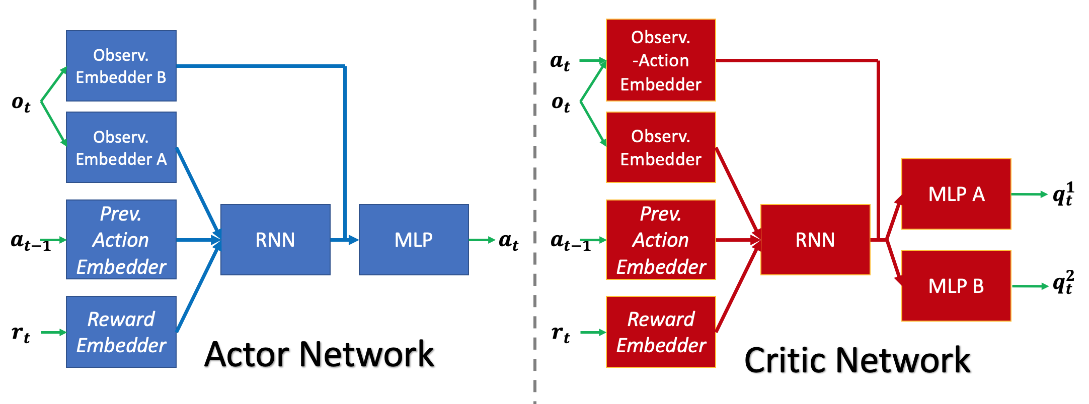
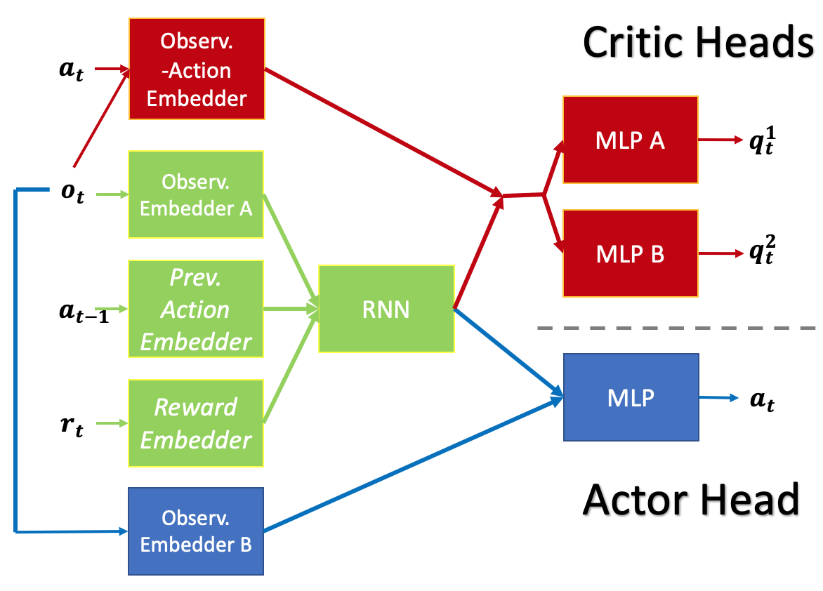
| Meta-RL | “Standard” | Robust RL | Generalization | Temporal | ||
| POMDP | in RL | credit assignment | ||||
| Hidden layer size | Observ. embedder | [32] | 2-layer CNN | |||
| Prev. Action embedder | [16] | not used | ||||
| Reward embedder | [16] | not used | ||||
| RNN | [128] | |||||
| MLP | [128,128,128] | [256, 256] | [128, 128] | |||
| RL hparams | Optimizer | Adam (Kingma & Ba, 2015) | ||||
| Learning rate | 3e-4 | |||||
| Discount factor | 0.99 | |||||
| Smoothing coef | 0.005 | |||||
| SAC(D) temperature | automatically updated by Haarnoja et al. (2018b) | 0.1 | ||||
| TD3 noises | default values from Fujimoto et al. (2018) | N/A | ||||
| Replay buffer size | 1e6 | |||||
| Batch size | 32 | 64 | 32 | |||
| RNN | Weight initialization | Orthogonal matrices (Saxe et al., 2014) | ||||
| Training hparams | Environment steps | 5M | 1.5M | 3M | 5M | |
| Gradient steps | 0.1M | 1.5M | 0.6M | 1.25M | ||
| Agent inputs | Largest input space | oard | oar | oa | oar | o |
| Best input space | oard | oa | o | o | o | |
| Meta-RL | Meta-RL | “Standard” | Robust RL | Generalization | Temporal | |
|---|---|---|---|---|---|---|
| POMDP | in RL | credit assignment | ||||
| Approach | Off-policy | On-policy | VRM | MRPO | EPOPT | IMPALA+SR |
| variBAD | variBAD | |||||
| Memory-based? | ✓ | ✓ | ✓ | ✗ | ✗ | ✓ |
| Off-policy? | ✓ | ✗ | ✓ | ✗ | ✗ | ✓ |
| Input space | oard | oard | oar | s | s | oar |
| Access to hidden states? | ✗ | ✗ | ✗ | ✓ | ✓ | ✗ |
Fig. 7 shows our (separate) recurrent actor-critic architecture (except for temporal credit assignment tasks). The shortcut from current observation embedding to the MLP may reduce the burden of accurately memorizing it in RNN, and is widely used in prior memory-based architectures (Zintgraf et al., 2020; Dorfman et al., 2020; Ding, 2019; Hung et al., 2018). For temporal credit assignment tasks (image-based observations, discrete actions), we adjust the network architectures: replace the MLP observation embedders in actor and critic with two-layer CNNs, remove the observation-action embedder in critic.
Table 5 shows the main hyperparameters we adopt for each benchmark. We did not tune these hyperparameters, except that we adjusted the number of gradient steps so that all the experiments could be completed in 72 hours.
We store the observed trajectories in the replay buffer we designed (see App. A). Each time we sample a (sub)trajectory given the context length. If the actual episode length is smaller than the context length, we zero-pad the (sub)trajectory. We use the zero start state strategy (Hausknecht & Stone, 2015; Kapturowski et al., 2019) for simplicity, i.e. use zeros as the initial hidden state of RNNs.
For Markovian policies (SAC and TD3), we remove the embedders and RNNs from the actor-critic architecture, and train them with same hyperparameters as those of recurrent policies. For each task, we report the results of either SAC or TD3, whichever achieves higher returns. For oracle policies, we use the well-tuned results from Table 1 (“SAC w/ unstructured row”) in Raffin et al. (2021) based on Stable Baseline3 (Raffin, 2020), for “standard” POMDPs. For the other benchmarks, we have to run the Markovian policies (SAC and TD3) with access to the hidden states, using the same training hyperparameters as those of recurrent policies. But these oracle policies might be not well-tuned given the same environment and gradient steps, especially in robust RL and generalization in RL. In temporal credit assignment benchmark, as the optimal value function is history-dependent, we do not run Markovian policies or oracle policies.
We also show the settings of the specialized methods we compared in the main paper in Table 6. Note that our recurrent model-free RL share exactly the same settings as off-policy variBAD (Dorfman et al., 2020) and VRM (Han et al., 2020). For MRPO (Jiang et al., 2021) and EPOPT (Rajeswaran et al., 2017a), they adopt totally different settings, i.e. on-policy Markovian approaches to MDPs (with access to the ground-truth state (s) of environment). Thus, in fact, MRPO and EPOPT should be viewed more as oracle policies as upper bounds of recurrent model-free RL.
Appendix C Evaluation Details
Throughout the experiments, we run each instance/variant in our implementation and each compared method with 4 random seeds.
There are two steps to select the best single variant of our implementation in each benchmark. First, we calculate the final performance of each variant by the average performance of the last 20% environment steps across the 4 seeds. Then we select the best variant in terms of the normalized returns, calculated by , where is the raw average return of that variant and and are the maximum and minimum of all the methods including oracle policy and random policy.
Appendix D Benchmark Details
We conduct our experiments on 6 benchmarks with 21 environments in total.
D.1 “Standard” POMDP Benchmark from VRM
We adopt the occlusion benchmark proposed by VRM, replace the deprecated roboschool with PyBullet (Coumans & Bai, 2016) as suggested by the official github repository333https://github.com/openai/roboschool#deprecated-please-use-pybullet-instead. We follow the practice in VRM (Han et al., 2020) in the other aspects of environment design, i.e. we remove all the position/angle-related entries in the observation space for “-V” environments and velocity-related entries for “-P” environments, to transform the original MDP into POMDP.
We also consider the classic Pendulum environment for sanity check in App. E.3.
Pendulum, Ant, Cheetah, Hopper, Walker-P.
The “-P” stands for the environments that keep position-related entries by removal of velocity-related entries. Thus, the observed state includes positions , while the hidden state is the velocities .
Pendulum, Ant, Cheetah, Hopper, Walker-V.
The “-V” stands for the environments that keep velocity-related entries by removal of position-related entries. Thus, the observed state includes positions , while the hidden state is the velocities .
D.2 Meta-RL Benchmark from Off-Policy VariBAD
For a fair comparison with the same training setting, we directly use the benchmark adopted in off-policy variBAD (Dorfman et al., 2020), and limit the number of training tasks as it does.
Semi-Circle.
The observed state includes the agent’s 2D position , and the hidden state is referred to the goal state . The goal state only appears in reward function: . The dynamic function is independent of the goal state.
Wind.
We modified the parameters of Wind environment in Dorfman et al. (2020) to make it harder to solve. The agent must navigate to a fixed (but unknown) goal within a distance of from its fixed initial state. Similarly to Semi-Circle, the reward function is goal conditioned but without hidden state: . The hidden state appears in the deterministic dynamics as a noise term, i.e. , where is sampled from at the initial time-step and then kept fixed.
Cheetah-Vel.
It uses MuJoCo (Todorov et al., 2012) simulator of HalfCheetah-v2. The hidden state is the target speed and the observed state includes the velocity . Reward function includes both the hidden state and action: . The dynamic function is independent of the goal state.
D.3 Meta-RL Benchmark from On-Policy VariBAD
For a fair comparison with the same training setting, we directly use the benchmark adopted in on-policy variBAD (Zintgraf et al., 2020), and do not limit the number of training tasks as it does.
{Ant, Cheetah, Humanoid}-Dir.
It uses MuJoCo (Todorov et al., 2012) simulator of Ant-v2, HalfCheetah-v2, Humanoid-v2. The hidden state is the target velocity direction , and the observed state includes the velocity . The reward function takes both the hidden state and action as inputs: where is the penalty constant. The dynamic function is independent of the goal state. Ant-Dir and Cheetah-Dir have only 2 tasks (forward or backward), while Humanoid-Dir samples tasks uniformly from the unit circle.
D.4 Robust RL Benchmark from MRPO
Hopper, Walker, Cheetah-Robust.
We directly adopt the environments used in MRPO (Jiang et al., 2021). In each environment, the hidden state is the dynamics parameters including the density and friction coefficients of the simulated robot in roboschool, adapted from the SunBlaze (Packer et al., 2018). The exact ranges of the hidden states in each environment can be found in Jiang et al. (2021, Table 1). We evaluate the algorithms with 100 tasks in each environment, and use the average of them as average returns, and the average of the worst of them as worst returns, following the MRPO paper.
D.5 Generalization in RL Benchmark from SunBlaze
Hopper, Cheetah-Generalize.
We directly adopt the environments used in SunBlaze (Packer et al., 2018). In each environment, the hidden state is the dynamics parameters including the density, friction coefficients, and the power of the simulated robot in roboschool. The exact ranges of both interpolation and extrapolation in the hidden state distribution for each environment can be found in Packer et al. (2018, Table 1). We follow the practice of SunBlaze to evaluate the interpolation and extrapolation success rates.
D.6 Temporal Credit Assignment Benchmark from IMPALA+SR
Delayed-Catch, Key-to-Door.
We directly adopted the two environments from IMPALA+SR paper (Raposo et al., 2021, Sec. 3.2 and 3.3). In both environments, they have discrete action spaces (3 and 4 actions) and pixels as observations ( and ). The reward functions are trajectory-level and sparse.
In Delayed-Catch, there are 40 runs in each episode, with a total length of around 280. The agent will only receive a non-zero reward at the end of each episode, which is the total number of successful runs, thus the optimal terminal reward is 40.
In Key-to-Door, there are three phases in one episode. In the first phase, the agent can pick up a key, but no reward will be given. In the second phase, the agent can pick up apples to get rewards. In the third phase, the agent can open the door, only if it has picked up the key in the first phase (the agent cannot see the key after the first phase), to get a reward bonus. Thus the final reward bonus depends on the agent’s action that happens in the distant past. We follow the prior work to report the success rate of opening the door as the evaluation metric.
Appendix E Full Experimental Results
E.1 Learning Curves of All the Compared Methods
In this subsection, we show all the learning curves of all the compared methods (including oracle policy as upper bound, Markovian and random policies as lower bounds) in each benchmark, namely “standard” POMDPs (Fig. 9 and Fig. 10), meta-RL (Fig. 11 and Fig. 12), robust RL (Fig. 13), generalization in RL (Fig. 14), and temporal credit assignment (Fig. 15).
| Benchmark | Best single variant | Environment | Env steps | Metric | Performance |
| “Standard” POMDP | td3-gru-64-oa-separate | Ant-P | 1.5M | Avg return | 348 282 |
| Ant-V | 1113 360 | ||||
| Cheetah-P | 2693 219 | ||||
| Cheetah-V | 1980 143 | ||||
| Hopper-P | 2133 326 | ||||
| Hopper-V | 1495 381 | ||||
| Walker-P | 982 339 | ||||
| Walker-V | 121 52 | ||||
| Meta-RL | td3-lstm-64-ord-separate | Semi-Circle | 1.5M | Avg return | 94.2 0.6 |
| td3-lstm-64-oad-separate | Wind | 0.75M | 62.8 0.5 | ||
| td3-lstm-64-oard-separate | Cheetah-Vel | 5M | -84.7 11.1 | ||
| sac-gru-max-oard-separate | Ant-Dir | 30M | 1886 177 | ||
| Cheetah-Dir | 20M | 4189 282 | |||
| Humanoid-Dir | 30M | 1322 257 | |||
| Robust RL | td3-lstm-64-o-separate | Cheetah-Robust | 3M | Avg return | 2278 454 |
| Worst return | 1587 355 | ||||
| Hopper-Robust | Avg return | 2392 127 | |||
| Worst return | 1169 304 | ||||
| Walker-Robust | Avg return | 1807 347 | |||
| Worst return | 766 504 | ||||
| Generalization in RL | td3-lstm-64-o-separate | Cheetah-Generalize | 3M | Interpolation | 0.989 0.008 |
| Extrapolation | 0.656 0.011 | ||||
| Hopper-Generalize | Interpolation | 0.757 0.138 | |||
| Extrapolation | 0.299 0.029 | ||||
| Temporal credit assignment | sacd-lstm-max-o-separate | Delayed-Catch | 2.5M | Avg return | 39.8 0.4 |
| Key-to-Door | 4M | Success rate | 0.996 0.009 |
E.2 Single Factor Analysis on Our Implementation
Our analysis will focus on ablating the important design decisions: the actor-critic architecture (Arch), the agent input space (Inputs), the underlying model-free RL algorithm (RL), the RNN encoder (Encoder), and the RNN context length (Len).
From these plots, we can see that each decision factor can make a difference in some environments. For example, the choice of RL algorithm is crucial in Ant-P (Fig. 16), Cheetah-V (Fig. 17), Wind (Fig. 18) and Hopper-Generalize (Fig. 20). The context length is essential in all the “-P” environments (Fig. 16), Cheetah-Vel (Fig. 18), and both the generalization environments (Fig. 20). The agent input space can make a difference in most “-P” environments (Fig. 16) possibly because oar contains the information of missing velocities.
E.3 Additional Results on Separate vs Shared Recurrent Actor-Critic Architecture
Now we show the result in another POMDP environment, Pendulum-V, which occludes the positions and angles, in Fig. 21. We can see that the shared encoder architecture is also worse than the separate one, possibly due to the different gradient scales in actor and critic losses w.r.t. the encoder.
E.4 Additional Results on Comparison with VRM
Both Fig. 1 and Fig. 22 shows the final performance of the same single variant of our implementation, but the former shows our results with 1.5M simulation steps while the latter shows our results with 0.5M simulation steps to match with those of VRM due to the time budget.
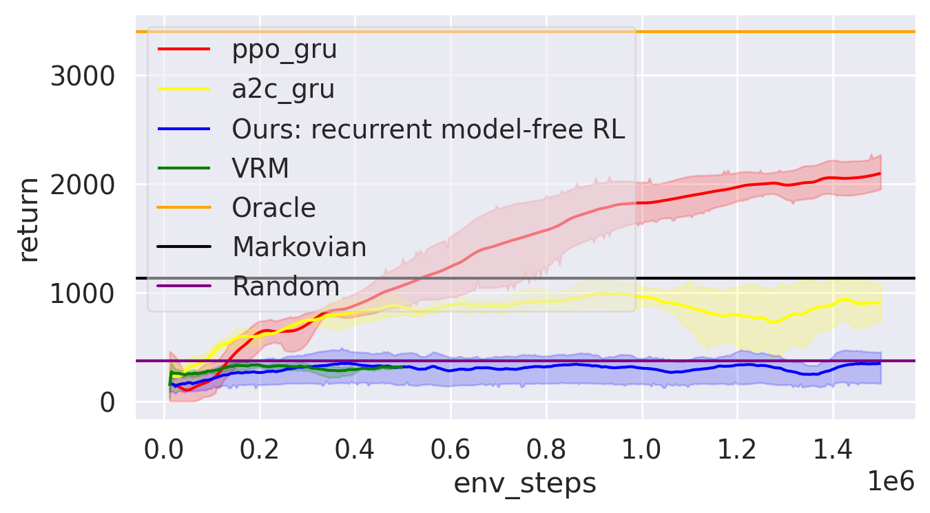

| Ant-P | Cheetah-P |
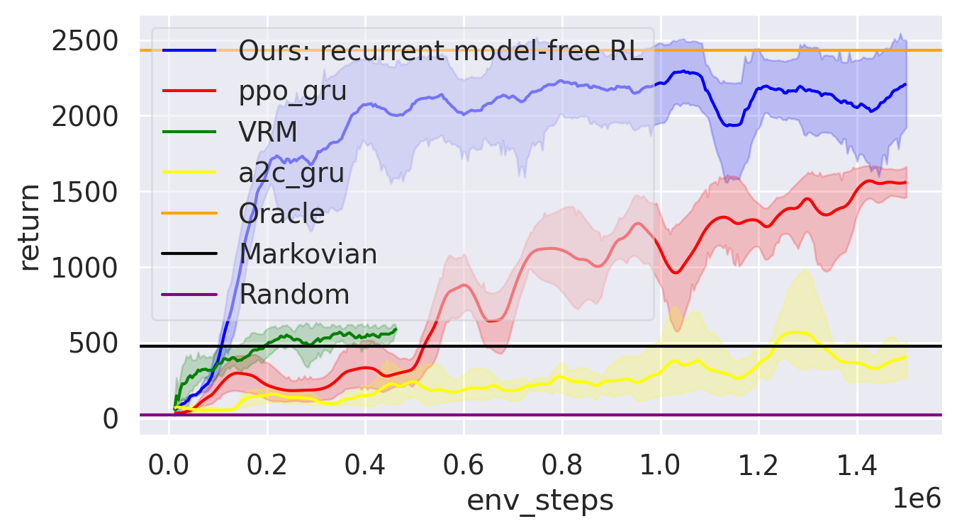
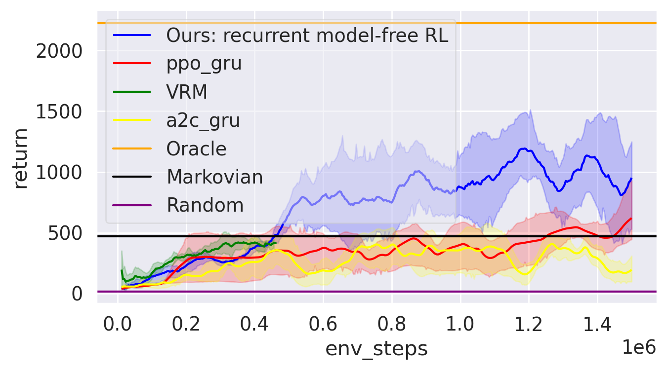
| Hopper-P | Walker-P |
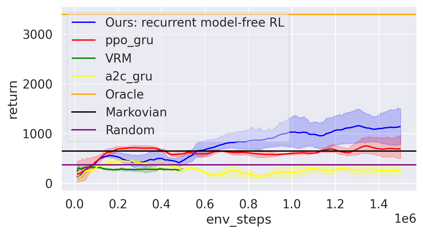

| Ant-V | Cheetah-V |
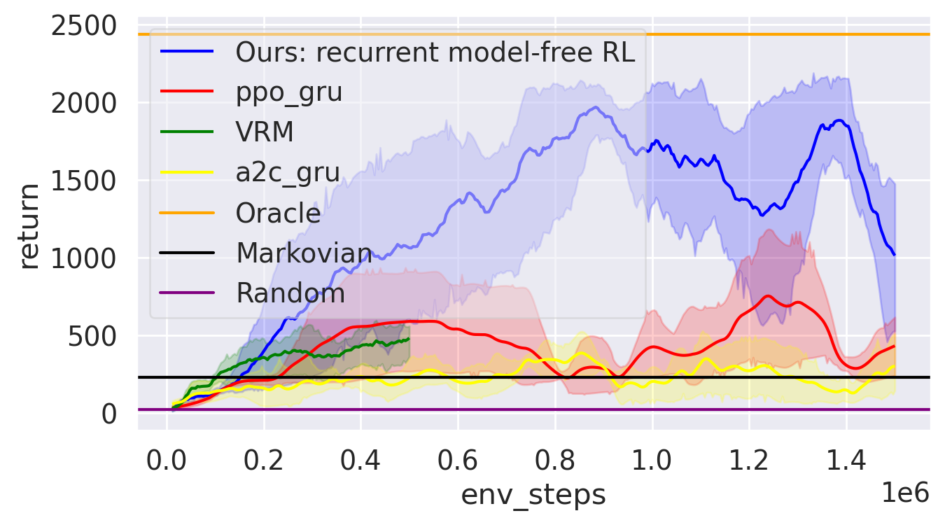
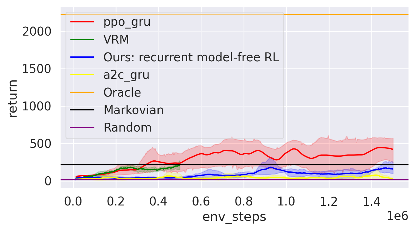
| Hopper-V | Walker-V |


| Semi-Circle | Wind |
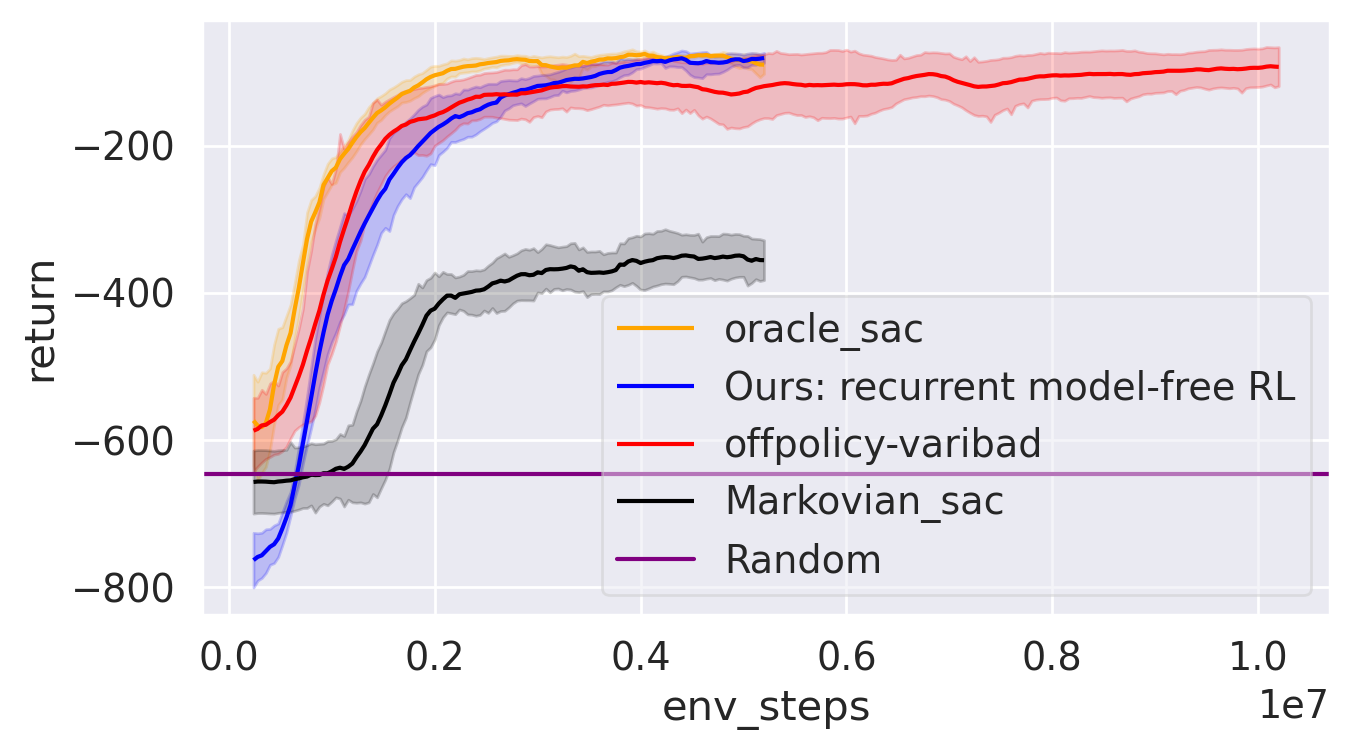
Cheetah-Vel


| Cheetah-Dir | Ant-Dir |

Humanoid-Dir

Hopper-Robust

Cheetah-Robust

Walker-Robust

Hopper-Generalize

Cheetah-Generalize


| Delayed-Catch | Key-to-Door |
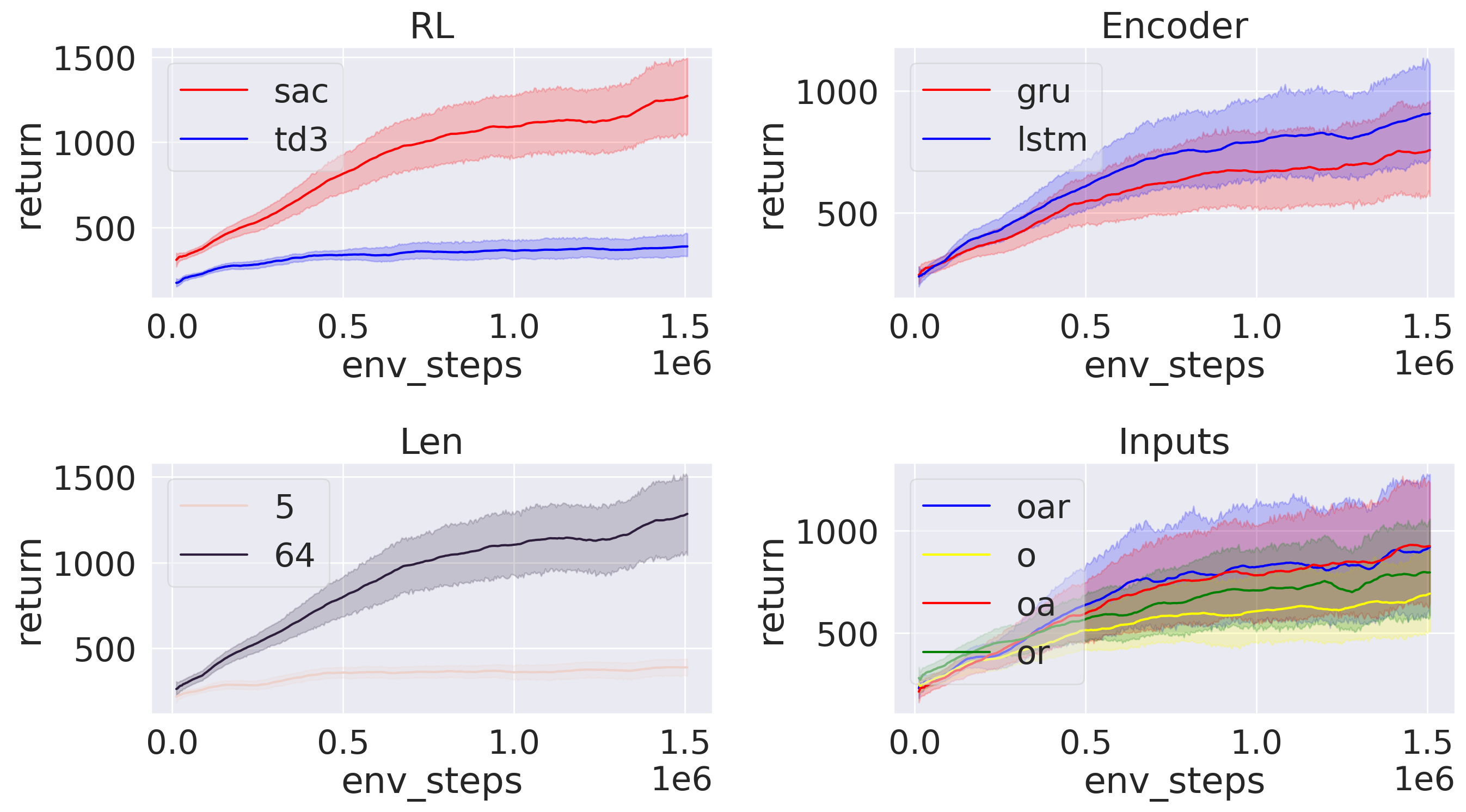
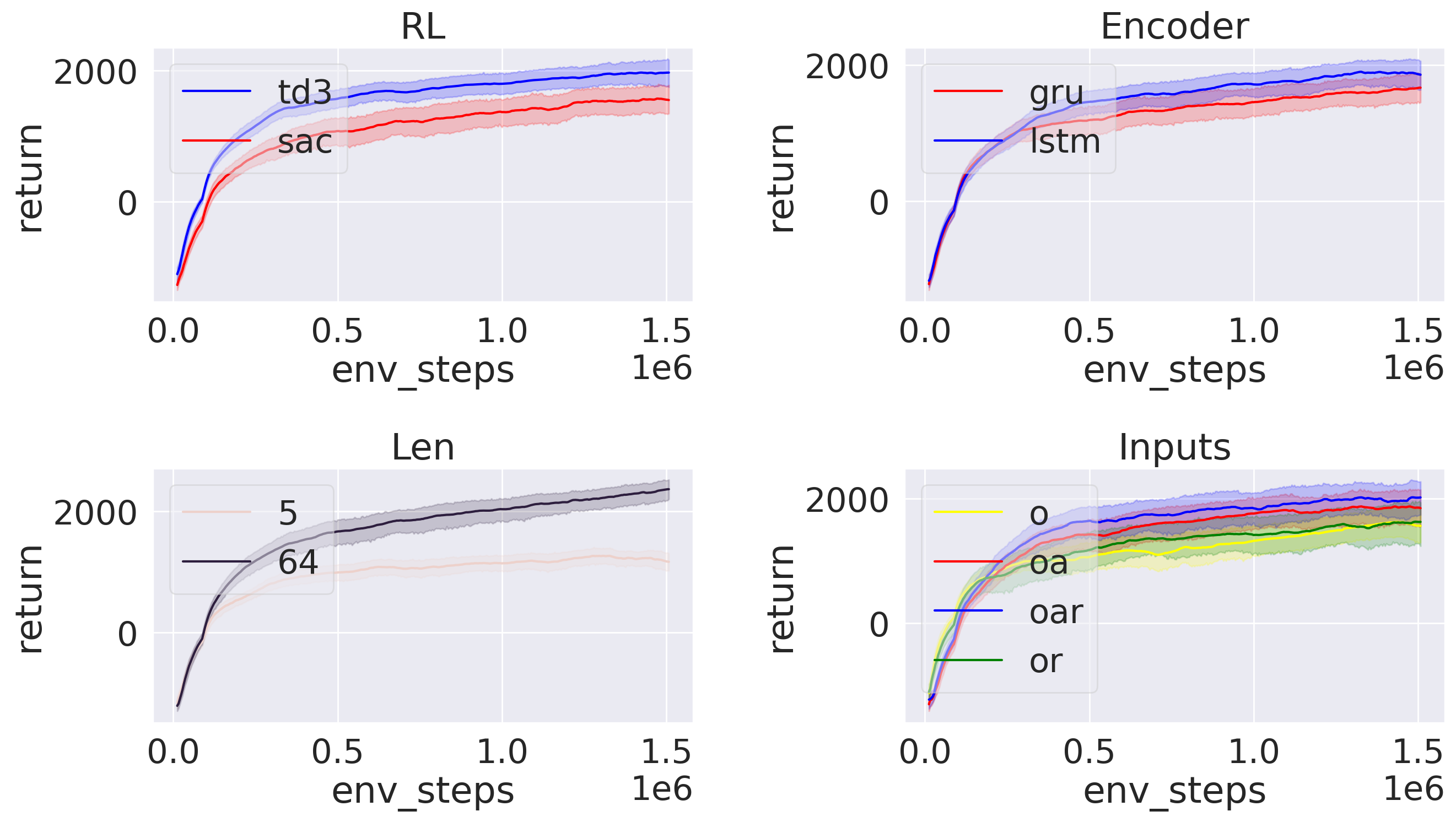
| Ant-P | Cheetah-P |
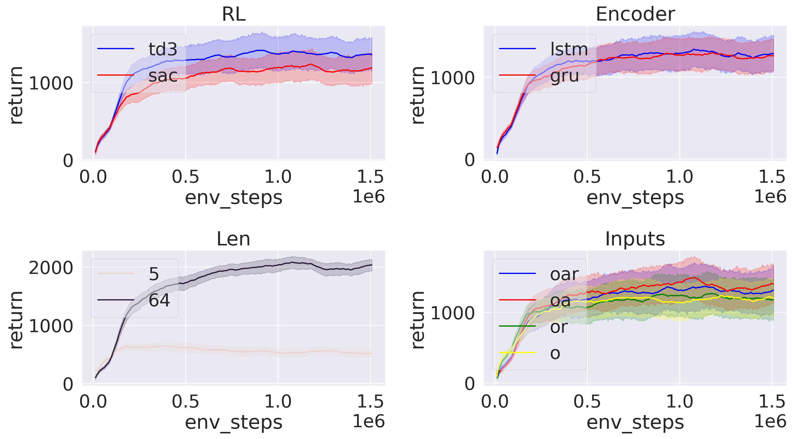
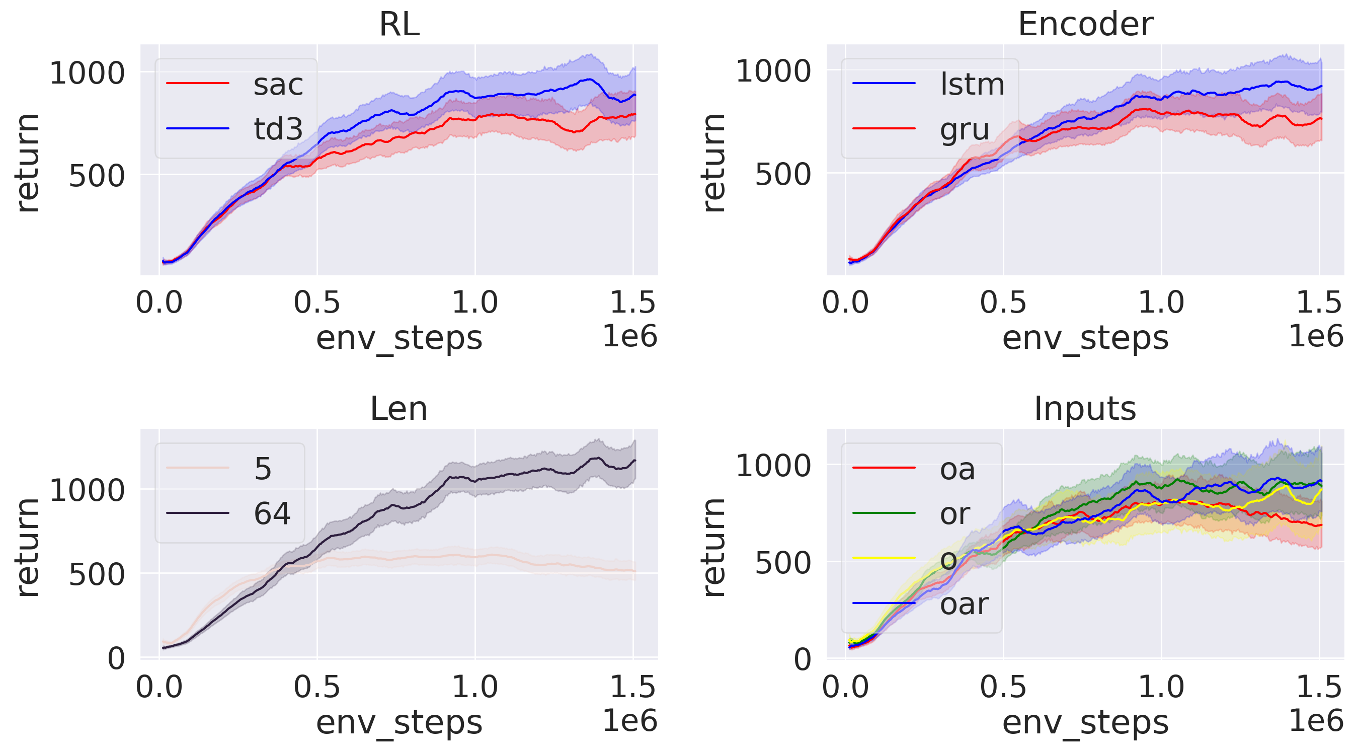
| Hopper-P | Walker-P |
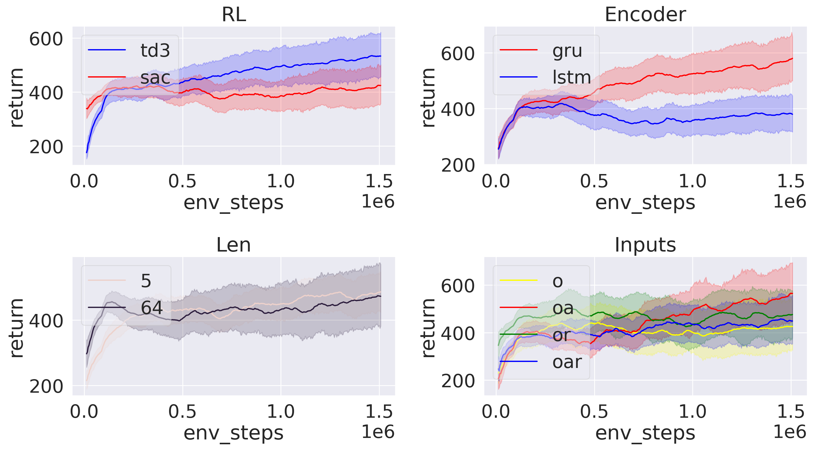
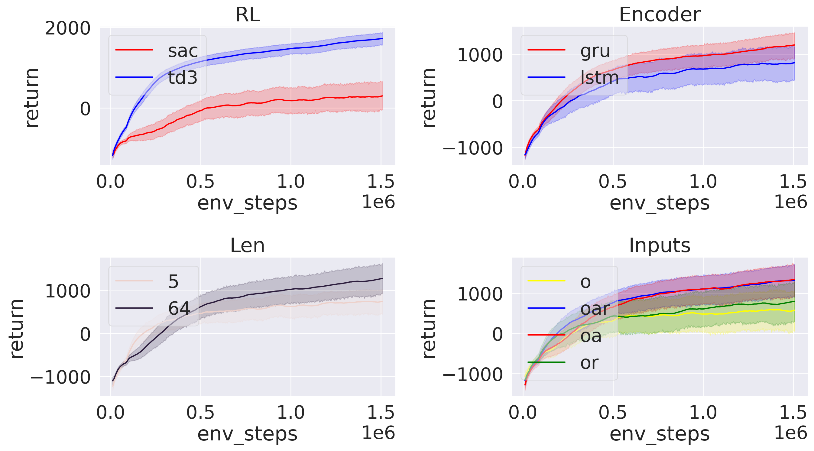
| Ant-V | Cheetah-V |
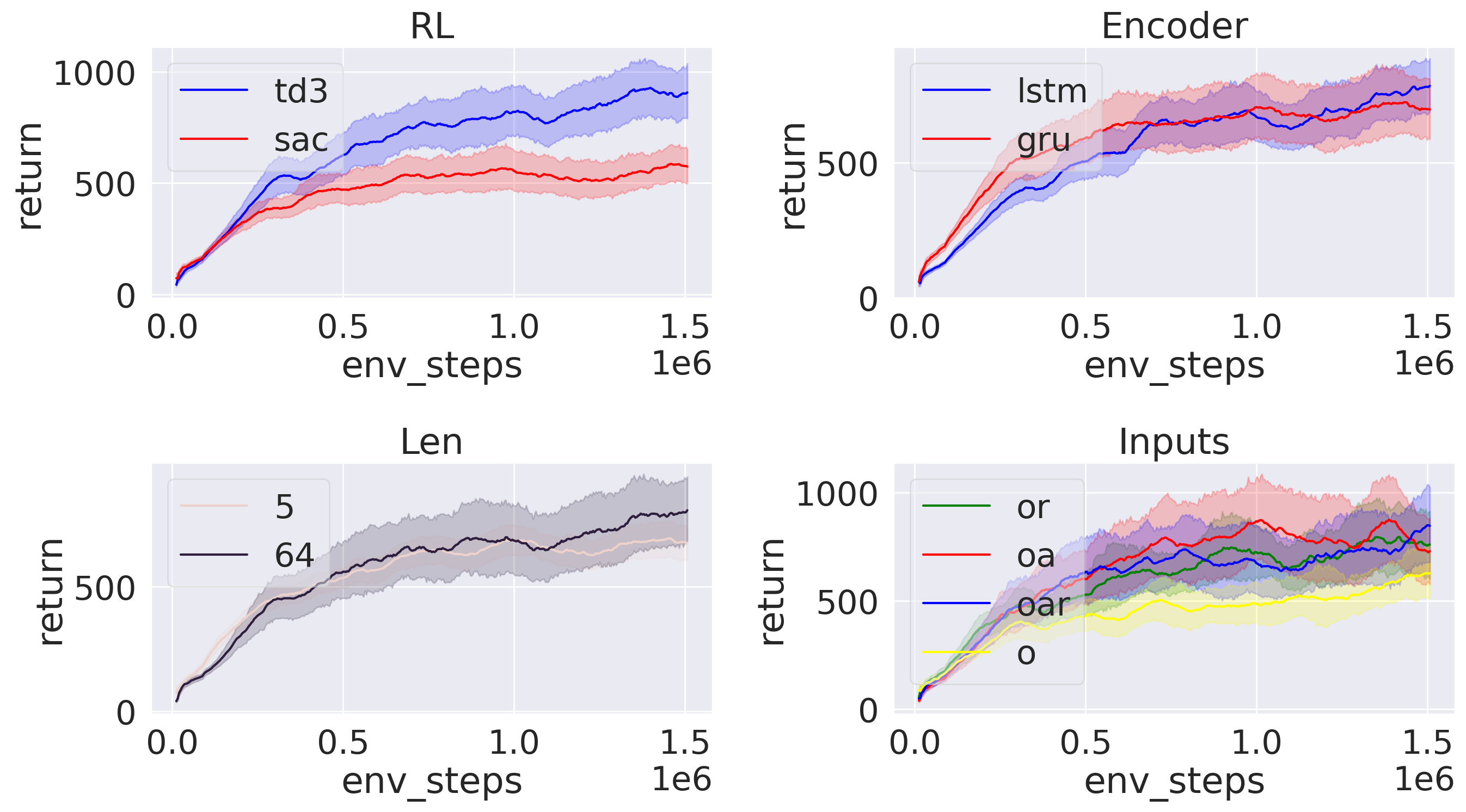
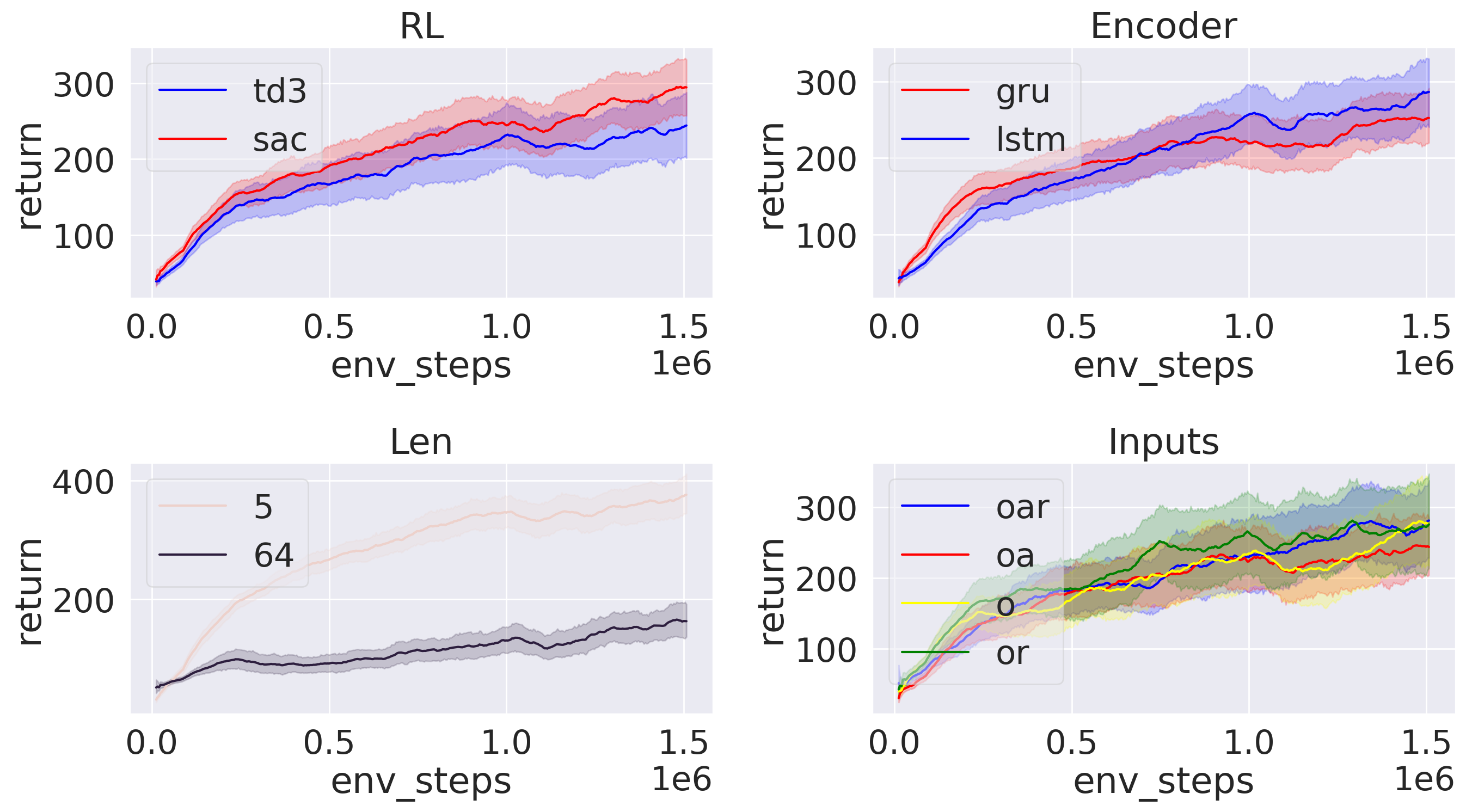
| Hopper-V | Walker-V |
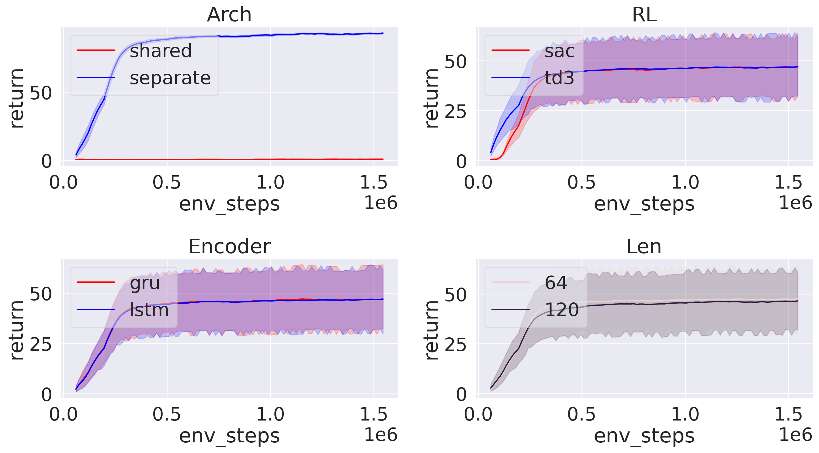
Semi-Circle
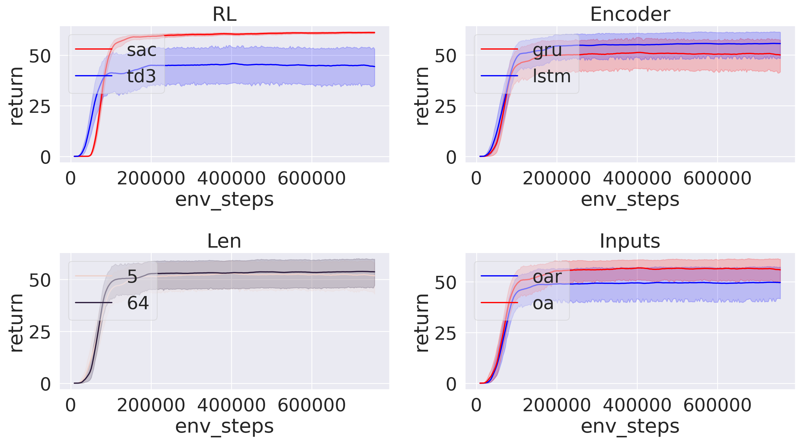
Wind
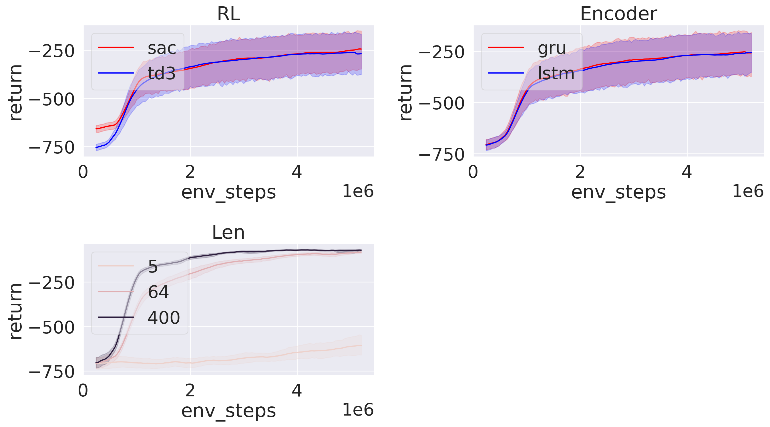
Cheetah-Vel
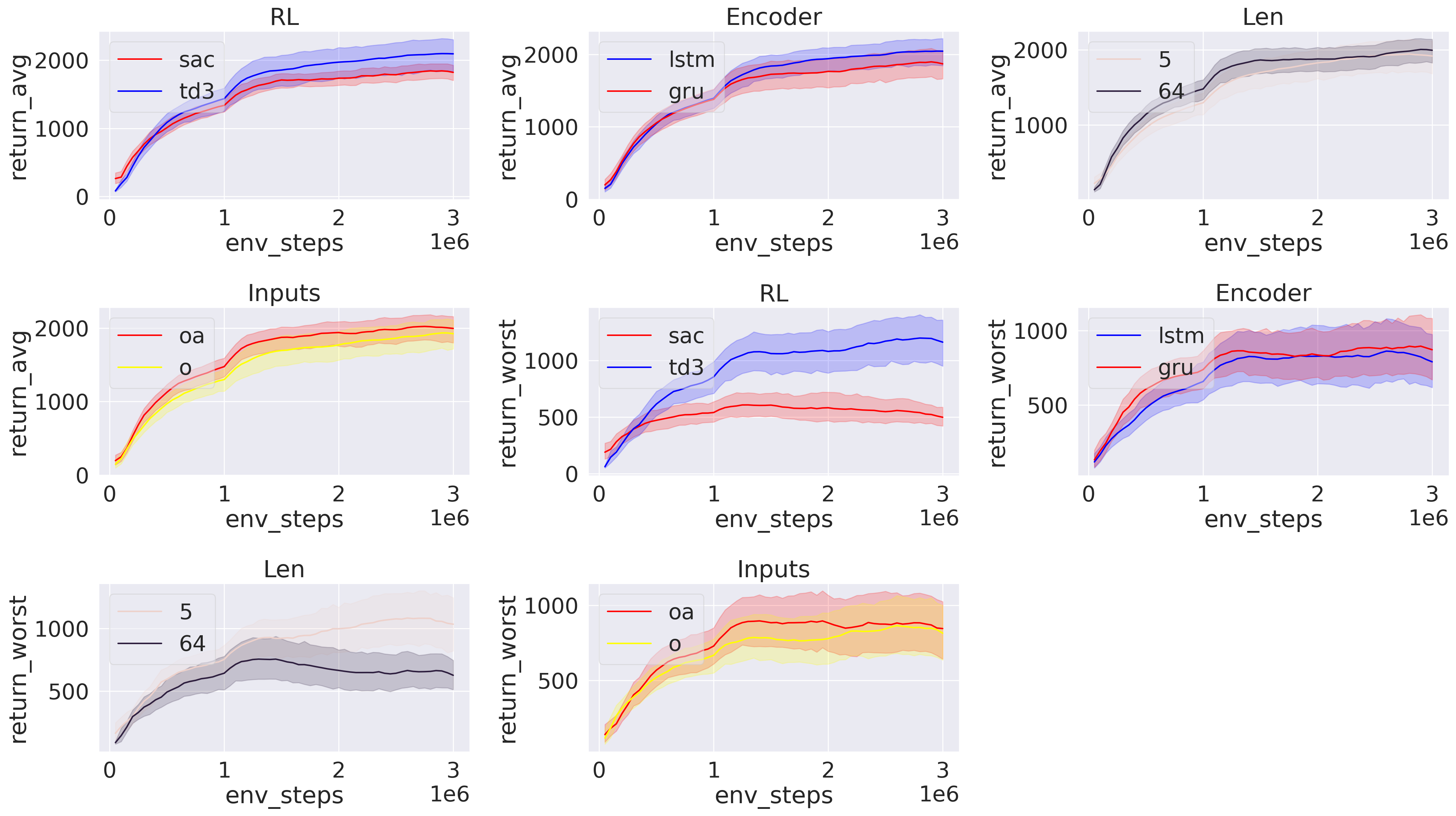
Hopper-Robust
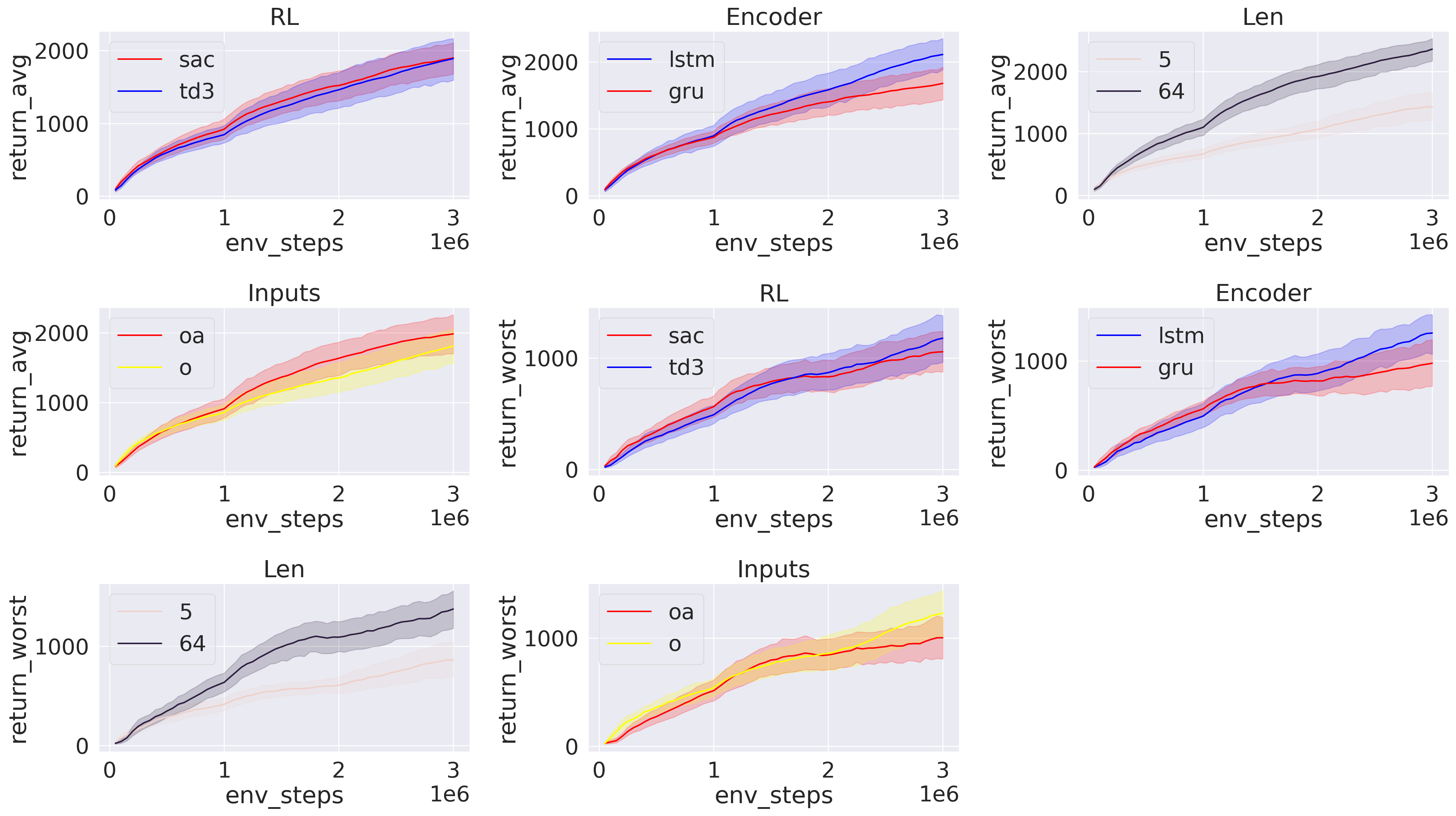
Cheetah-Robust
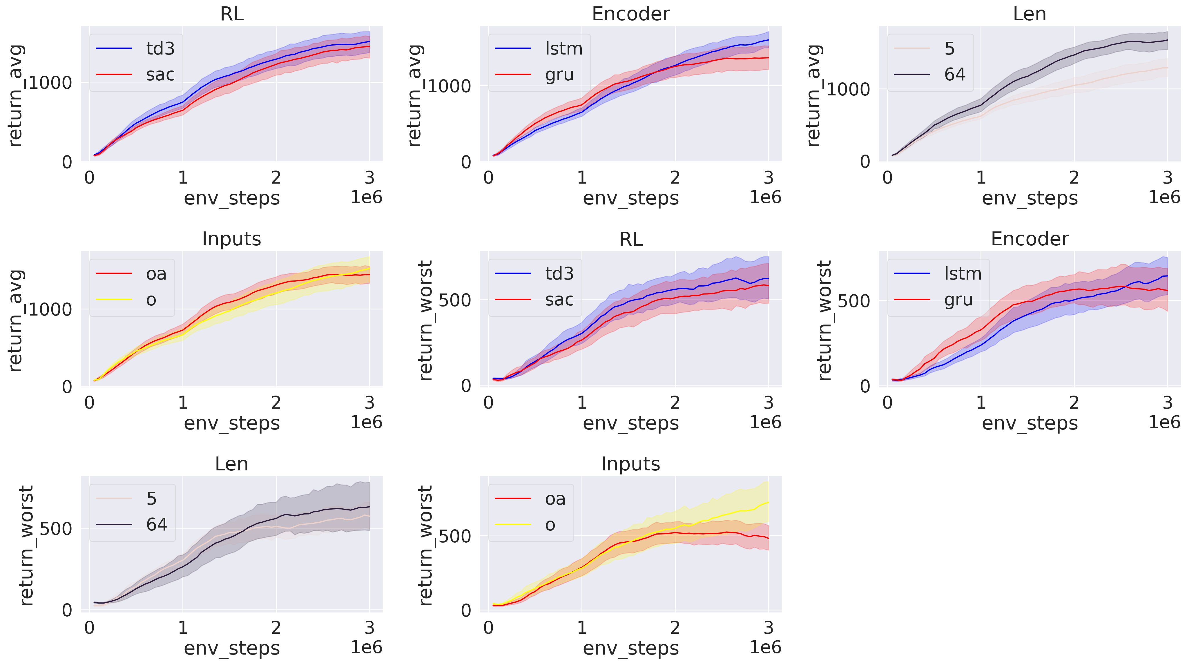
Walker-Robust
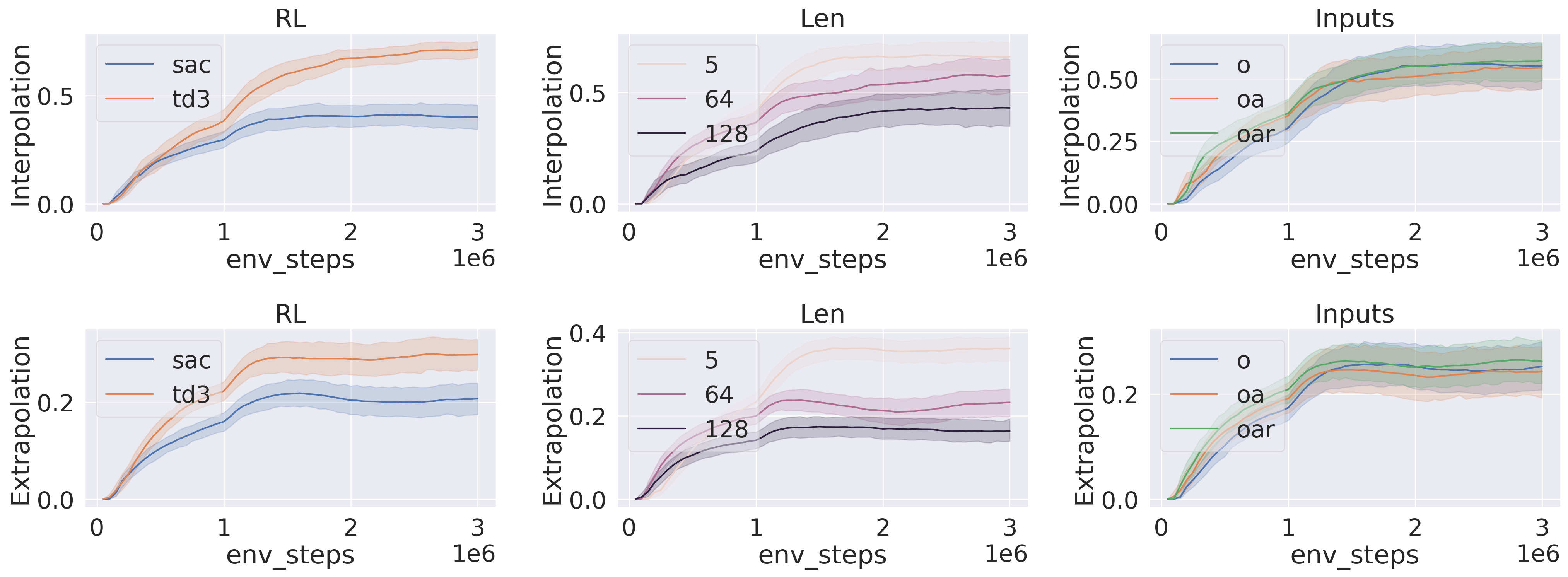
Hopper-Generalize
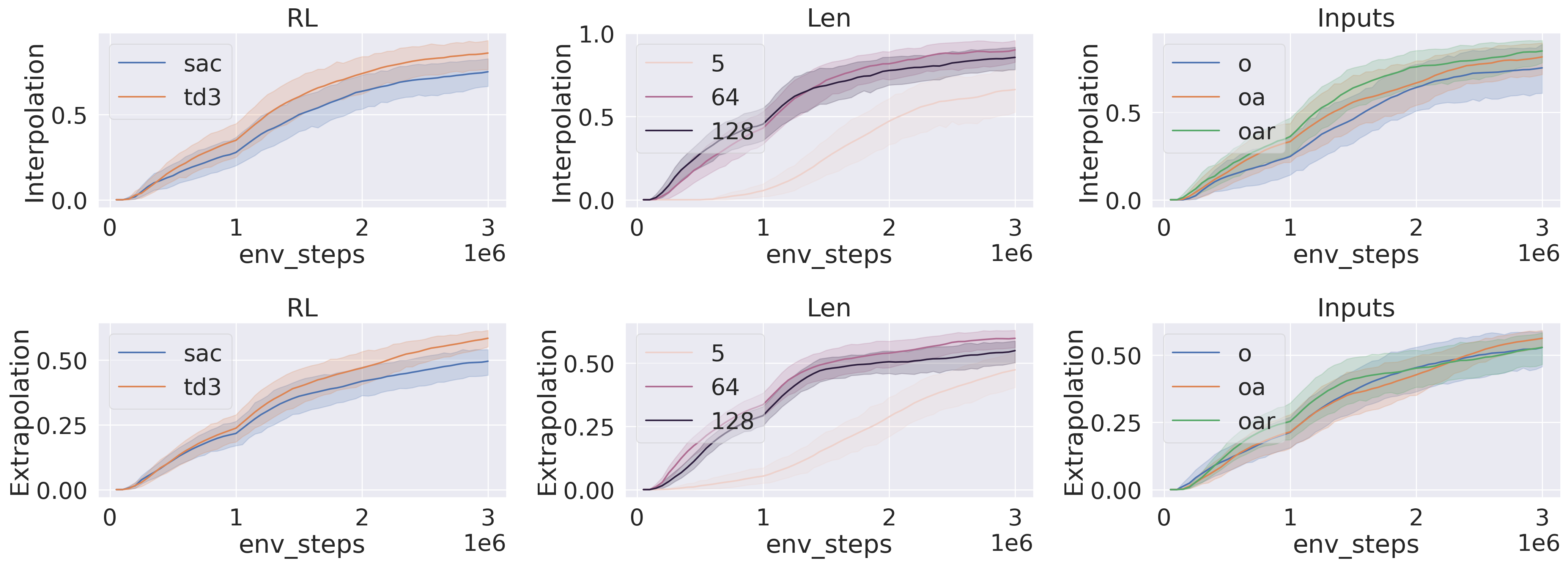
Cheetah-Generalize

