Convergence of Random Reshuffling Under
The Kurdyka-Łojasiewicz Inequality

Abstract

We study the random reshuffling (RR) method for smooth nonconvex optimization problems with a finite-sum structure. Though this method is widely utilized in practice, e.g., in the training of neural networks, its convergence behavior is only understood in several limited settings. In this paper, under the well-known Kurdyka-Łojasiewicz (KL) inequality, we establish strong limit-point convergence results for RR with appropriate diminishing step sizes, namely, the whole sequence of iterates generated by RR is convergent and converges to a single stationary point in an almost sure sense. In addition, we derive the corresponding rate of convergence, depending on the KL exponent and suitably selected diminishing step sizes. When the KL exponent lies in $[0,\frac{1}{2}]$, the convergence is at a rate of $\mathcal{O}(t^{-1})$ with $t$ counting the number of iterations. When the KL exponent belongs to $(\frac{1}{2},1)$, our derived convergence rate is of the form $\mathcal{O}(t^{-q})$ with $q\in(0,1)$ depending on the KL exponent. The standard KL inequality-based convergence analysis framework only applies to algorithms with a certain descent property. We conduct a novel convergence analysis for the non-descent RR method with diminishing step sizes based on the KL inequality, which generalizes the standard KL framework. We summarize our main steps and core ideas in an informal analysis framework, which is of independent interest. As a direct application of this framework, we establish similar strong limit-point convergence results for the reshuffled proximal point method.

90C30, 90C06, 90C26, 90C15

1 Introduction

In this paper, we consider the finite-sum optimization problem

(1) $$\operatorname*{\text{minimize}}_{x\in\mathbb{R}^{n}}~{}f(x)=\frac{1}{N}\sum_{i=1}^{N}f(x,i),$$

where each component function $f(\cdot,i):\mathbb{R}^{n}\to\mathbb{R}$ is continuously differentiable but not necessarily convex. Problem (1) appears frequently in various engineering fields such as machine learning and signal processing [19, 20]. This work aims at studying the random reshuffling (RR) method for solving problem (1). In the next subsection, we first introduce RR and its special case, the incremental gradient method, in detail and then discuss motivational background for RR.

1.1 The Random Reshuffling Method

We now review the core procedures of RR. First, let us define the set of all possible permutations of $\{1,2,\ldots,N\}$ as

(2) $$\Lambda:=\{\sigma:\sigma\text{ is a permutation of }\{1,2,\ldots,N\}\}.$$

At each iteration $t$, a permutation $\sigma^{t}$ is generated according to an i.i.d. uniform distribution over $\Lambda$. Then, RR updates $x^{t-1}$ to $x^{t}$ through $N$ consecutive gradient descent-type steps by using the components $\{f(\cdot,\sigma^{t}_{1}),\ldots,f(\cdot,\sigma^{t}_{N})\}$ sequentially, where $\sigma^{t}_{i}$ represents the $i$-th element of $\sigma^{t}$. In each step, only one component $f(\cdot,\sigma^{t}_{i})$ is selected for updating. To be more specific, this method starts with $\tilde{x}^{t}_{0}=x^{t-1}$ and then uses $f(\cdot,\sigma^{t}_{i})$ to update $\tilde{x}^{t}_{i}$ as

(3) $$\tilde{x}^{t}_{i}=\tilde{x}^{t}_{i-1}-\alpha_{t}\nabla f(\tilde{x}^{t}_{i-1},\sigma^{t}_{i})$$

for $i=1,2,\ldots,N$, resulting in $x^{t}=\tilde{x}^{t}_{N}$. The code of RR is shown in Algorithm 1.

Algorithm 1 RR: Random Reshuffling

0:  Choose an initial point $x^{0}\in\mathbb{R}^{n}$;

1:  Set iteration count $t=1$;

2:  while stopping criterion not met do

3:     Update the step size $\alpha_{t}$ according to a certain rule;

4:      Generate a uniformly random permutation $\sigma^{t}$ of $\{1,\ldots,N\}$;

5:     Set $\tilde{x}_{0}^{t}=x^{t-1}$;

6:     for $i=1,2,\ldots,N$ do

7:        Update the inner iterate via $\tilde{x}_{i}^{t}=\tilde{x}_{i-1}^{t}-\alpha_{t}\nabla{f}(\tilde{x}_{i-1}^{t},\sigma^{t}_{i})$;

8:     end for

9:     Set $x^{t}=\tilde{x}_{N}^{t}$;

10:     Update iteration count $t=t+1$;

11:  end while

A special case of RR is the so-called incremental gradient method (IG), which uses $\sigma^{t}=\{1,2,\ldots,N\}$ for all $t\geq 0$. Thus, it updates $x^{t-1}$ to $x^{t}$ through (3) by utilizing the components $\{f(\cdot,1),\ldots,f(\cdot,N)\}$ sequentially. Hence, all our subsequent conclusions for RR naturally apply to the incremental gradient method.

Motivations. One classical algorithm for addressing problem (1) is the gradient descent method. However, in many modern large-scale applications, a fundamental challenge of problem (1) is that the number of components $N$ can be extremely large. Therefore, using the full information of $f$ (say the full gradient of $f$) in each update can be computationally prohibitive. This observation is precisely one of the main motivations of RR, which is tailored to modern large-scale optimization problems with finite-sum structure. In contrast to the standard gradient descent method, RR performs a gradient descent-type step in each update by using the gradient of only one component function rather than all the components of $f$. In terms of empirical performance, it has been reported that RR can outperform the gradient descent method for large-scale instances of problem (1); see [7] for more details.

Another popular and ubiquitous algorithm for solving problem (1) is the stochastic gradient method (SGD) [49]. Though SGD is widely studied in theory, what is commonly implemented in practice is actually RR [18, 50, 40, 27]. Indeed, RR is also known as “SGD without replacement” [50, 40]. The superiority of RR over SGD mainly stems from the following observations: 1) The random reshuffling sampling scheme is easier and faster to implement than the i.i.d. random sampling required in SGD. 2) RR utilizes all the data points in each epoch and hence, often has better theoretical and empirical performance. As a result of this superiority, RR has been included in well-known software packages such as PyTorch [45] and TensorFlow [1] as a fundamental solver and is used in a vast variety of engineering fields. Most notably, RR is extensively applied in practice for training deep neural networks; see, e.g., [7, 25, 27, 40, 43]. These special instances of RR and IG are part of the family of backpropagation algorithms for the training of neural networks [7].

Although RR enjoys vast applicability in practice, its convergence behavior is primarily studied under strong convexity; see, e.g., [25]. This restrictive setting is mainly motivated by the claim that RR significantly outperforms SGD for strongly convex problems. In this work, we will establish much broader convergence results for RR under the Kurdyka-Łojasiewicz (KL) inequality. We summarize our main contributions below.

1.2 Main Contributions

In order to compare different convergence results, we adopt the terminologies “strong limit-point convergence” and “weak convergence” used in [2]. Here, weak convergence means $\lim_{t\to\infty}\|\nabla f(x^{t})\|=0$, while strong limit-point convergence requires the whole sequence of iterates to converge to a single limit point and this limit point is a stationary point of (1).

We study RR (see Algorithm 1) for solving problem (1). Our ultimate goal is to understand the convergence behavior of this algorithm under the so-called Kurdyka-Łojasiewicz (KL) inequality of $f$ (see Definition 2.1). With the standard Lipschitz continuous gradient assumption (see Section 2.2) and the mild KL assumptions (see Equation 9), we establish strong limit-point convergence results for RR equipped with proper diminishing step sizes (see Theorems 3.10 and 3.18). That is, the whole sequence of iterates $\{x^{t}\}_{t\geq 1}$ generated by Algorithm 1 converges to a stationary point $x^{*}$ of $f$ in an almost sure sense. Next, under the same setting, we establish the corresponding rate of convergence (see Theorems 3.16 and 3.18), which will depend on the KL exponent $\theta$ of $f$ (see (35)) and on the selected step sizes $\{\alpha_{t}\}_{t\geq 1}$. With a suitable choice of the diminishing step sizes $\{\alpha_{t}\}_{t\geq 1}$, our rate results can be summarized as:

• If $\theta\in[0,\frac{1}{2}]$ at the target stationary point $x^{*}$, then $\{x^{t}\}_{t\geq 1}$ will converge to $x^{*}$ at a rate of $\mathcal{O}(t^{-1})$. Remarkably, this rate matches the best available rate for ${\sf RR}$ obtained in strongly convex optimization; see, e.g., [25].

• If $\theta\in(\frac{1}{2},1)$ at $x^{*}$, then $\{x^{t}\}_{t\geq 1}$ will converge to $x^{*}$ at a rate of $\mathcal{O}(t^{-q})$ with $q\in(0,1)$ depending on the KL exponent $\theta$.

A more detailed discussion of the possible rates of convergence and their dependence on the KL exponent $\theta$ and step sizes $\{\alpha_{t}\}_{t\geq 1}$ is given in Section 3.4. As a standard byproduct of the KL inequality-based analysis, all our convergence results apply to the last iterate of Algorithm 1. Our results extend the convergence analysis of RR from the strongly convex regime to a much more general nonconvex setting. To the best of our knowledge, all the above results are new for RR.

RR is a non-descent method. It can be viewed as a gradient descent method with an additional error term that is proportional to the step size [9, 25] and requires diminishing step sizes to ensure convergence. Therefore, the standard KL inequality-based analysis developed in [2, 5, 4, 6, 14]—which applies to algorithms that possess a certain sufficient decrease property—is not directly applicable here. Different to the standard KL framework, through invoking proper diminishing step sizes, we utilize a more elementary analysis to first establish weak convergence results that allows to avoid the sufficient decrease property. Then, by accumulating the potential ascent (i.e., error terms) of each step of RR, we derive a novel auxiliary descent-type condition for the iterates. Based on this auxiliary condition, we combine the standard KL analysis framework and the dynamics of the diminishing step sizes to establish strong limit-point convergence results and derive the corresponding rate of convergence depending on the KL exponent $\theta$. Thus, our results generalize the standard KL analysis framework to cover a class of non-descent methods with diminishing step sizes. We summarize our main steps and core ideas in an informal analysis framework in Section 4.1, which is of independent interest. As a direct application of this new KL analysis framework, we show similar convergence results for another important shuffling-type algorithm—the reshuffled proximal point method (see Section 4.2).

We believe that our results and the general framework presented in Section 4.1 can also serve as a blueprint for the KL inequality-based convergence analysis of other non-descent methods with diminishing step sizes.

1.3 Connections to Previous Works

$\bullet$ The random reshuffling method. There have been numerous works studying RR for solving problem (1). In what follows, we will briefly review some representative results for these methods and provide the connections to our results.

As pointed out by various works, e.g., [7, 17, 25], RR is widely utilized in practice for tackling large-scale machine learning tasks such as training neural networks. The short note [17] shows empirical superiority of RR over SGD. Theoretically, understanding the observed superiority of RR over SGD remains an important problem. In [48], the authors conjectured a noncommutative arithmetic-geometric mean inequality that leads to a lower iteration complexity of RR than that of SGD for least-squares optimization. However, this conjecture was later proved to be not true in general [32]. Recently, under the assumptions that the objective function $f$ is strongly convex, each component function $f(\cdot,i)$ has a Lipschitz continuous Hessian, and the iterates generated by RR are uniformly bounded, Gürbüzbalaban et al. formally established that the whole sequence of q-suffix averaged iterates converges to the unique optimal solution at a rate of $\mathcal{O}({1}/{t})$ with high probability [25]. The authors also commented that this rate result of RR outperforms the min-max lower bound of the rate achieved by SGD for strongly convex minimization (i.e., $\Omega({1}/{\sqrt{t}})$; cf. [3, 41]). Initiated by these first insights, various works start to understand the properties of RR, but mainly focusing on iteration complexity results; see, e.g., [27, 40, 39, 43, 29]. For instance, under the assumptions that $f$ is strongly convex and $f$, the gradient of $f$, and the Hessian of $f$ are all Lipschitz continuous, the work [27] shows an $\mathcal{O}(1/T)$ iteration complexity result in expectation for the distances between the iterates and the unique optimal solution, where $T$ is the preset total number of iterations. Relaxations of the different and partly stringent Lipschitz continuity conditions used in [27] have been further discussed and investigated in [40, 39]. Note that there is not a direct way to compare our results to existing iteration complexity results since our KL inequality-based analysis is fundamentally different and describes asymptotic convergence behavior.

A common assumption imposed by the above mentioned works is that the objective function has to be strongly convex, which is typically not satisfied in many important applications. By contrast, our KL inequality-based convergence analysis applies to much more general nonconvex functions. Specifically, when the KL exponent equals to $\frac{1}{2}$ at the stationary point that RR converges to, the corresponding convergence rate will be $\mathcal{O}({1}/{t})$, which matches the rate of the strongly convex setting [25]. However, it should be noted that a function with a stationary point having KL exponent $\frac{1}{2}$ can generally be nonconvex as well.

As mentioned, RR also covers the well-known and popular IG method as a special case. In [38, 53, 51, 52], weak convergence results for IG (i.e., $\lim_{t\rightarrow\infty}\|\nabla f(x^{t})\|=0$) are provided under various step size schemes and different assumptions on the problem. A more recent work [26] shows that if $f$ is strongly convex and the iterates generated by IG are uniformly bounded, then the whole sequence of iterates will converge to the unique optimal solution at a rate of $\mathcal{O}(1/t)$. Our KL inequality-based analysis naturally extends these results for IG to a broader nonconvex setting.

$\bullet$ The KL inequality and the related convergence analysis framework. The Kurdyka-Łojasiewicz (KL) inequality plays a key role in our analysis. We refer to a series of important works for the rich theory and history of this property; see, e.g., [35, 36, 37, 30, 31, 11, 10, 12, 13]. The KL inequality is a powerful concept applicable to a large range of (nonconvex) functions arising in real-world problems; see [14, Section 5] for a discussion. A striking application of this inequality is to analyze the convergence (or the stronger finite length property) of the gradient flow in dynamical systems theory. Absil et al. [2] extended the analysis to obtain strong limit-point convergence of numerical optimization algorithms when used to optimize real analytical functions, where the algorithms are assumed to satisfy a certain sufficient decrease property. The results in [2] apply to the well-known gradient descent and trust region methods with appropriate line-search procedures. The KL inequality-based convergence analysis was then extended and popularized by Attouch and Bolte et al. [4, 5, 6, 14] for establishing the strong limit-point convergence of several descent methods for nonsmooth nonconvex optimization. In particular, the work [4] considers the proximal point method for minimizing functions satisfying the KL inequality and obtains strong limit-point convergence results and the corresponding rate of convergence based on the KL exponent. The strong limit-point convergence result was then shown for proximal coordinate-type (or alternating-type) gradient methods in [14] when optimizing the sum of a smooth nonconvex function and a nonsmooth one. Thanks to the aforementioned pioneering works, the strength of the KL inequality has been widely recognized in both optimization and engineering societies. Now, the KL inequality has become one of the main tools for understanding convergence properties of (mostly nonconvex) optimization algorithms.

The standard KL inequality-based convergence analysis crucially relies on the descent property of the algorithm. Let us take the analysis framework summarized in [14, Section 3.2] as an example. As a first step, the sufficient decrease property typically allows to show weak convergence. Then, by combining the sufficient decrease property, the weak convergence result, and the KL inequality, strong limit-point convergence as well as the corresponding rate of convergence can be established for the descent method in question. Most existing works follow this analysis framework to analyze descent algorithms. Besides, there is also a set of works considering methods that do not have a descent property on the objective function itself; see, e.g., the Douglas-Rachford splitting-type methods [34], inertial proximal gradient methods [44, 15] and its alternating version [46], alternating direction method of multipliers (ADMM) [33, 54, 16], to name a few. An almost universal proof strategy in these works is to construct a particular Lyapunov function (or merit function) for which the algorithm possesses a sufficient decrease property. Then, the standard KL framework can be utilized to derive strong limit-point convergence results. The price to pay here is to assume the KL inequality on the Lyapunov function rather than the original objective function. This compensation can be mild if the goal is only to obtain strong limit-point convergence of the sequence of iterates since the KL inequality holds for a vast class of functions. Nonetheless, determining the KL exponent of the Lyapunov function given the exponent of the original objective function can be non-trivial.

There are also a few works discussing the KL inequality-based analysis for descent-type methods with relative updating errors [24, 23]. The proof techniques in [24, 23] share certain similarities with our derivation for establishing the finite length result by invoking a summability condition on the relative errors (cf. our (31) and [23, Page 896]). However, the algorithms considered by Garrigos and Frankel et al. still satisfy a sufficient decrease property and utilize step sizes that are bounded away from zero. Hence, the analysis conducted in [24, 23] for obtaining weak convergence, strong limit-point convergence, and convergence rates follows the standard one [4, 14] and is different from our derivations.

To summarize, the existing works mainly consider algorithms that possess a sufficient decrease property either on the objective function itself or on a well constructed Lyapunov function. By contrast, RR is a non-descent method and requires diminishing step sizes to ensure convergence. Therefore, the standard KL inequality-based convergence analysis framework pioneered by the works [2, 4, 5, 6, 14] is not directly applicable here. Instead, we conduct a novel analysis by combining the standard KL framework and the dynamics of the diminishing step sizes to establish strong limit-point convergence results and the corresponding rate of convergence for RR. It is also worth emphasizing that our analysis only involves the KL inequality of the objective function itself. We refer to Section 4.1 for a more detailed summary.

2 Preliminaries and Assumptions

2.1 The Kurdyka-Łojasiewicz (KL) Inequality

We start with reviewing the basic elements of the KL inequality, which will serve as the key tool for our convergence analysis of RR. As we consider the case where the objective function $f$ in problem (1) is smooth, we now present the definition of the KL inequality tailored to smooth functions. More broadly, using appropriate subdifferentials, the KL inequality can be introduced for nonsmooth functions as well; see, e.g., [5, 4, 6, 14].

Definition 2.1 (KL inequality).

The function $f$ is said to satisfy the KL inequality at a point $\bar{x}\in\mathbb{R}^{n}$ if there exist $\eta\in(0,\infty],$ a neighborhood $U$ of $\bar{x}$, and a continuous and concave function $\varrho:[0,\eta)\to\mathbb{R}_{+}$ with

$$\varrho\in C^{1}((0,\eta)),\quad\varrho(0)=0,\quad\text{and}\quad\varrho^{\prime}(x)>0\quad\forall~{}x\in(0,\eta),$$

such that for all $x\in U\cap\{x:0<|f(x)-f(\bar{x})|<\eta\}$ the KL inequality holds, i.e.,

(4) $$\varrho^{\prime}(|f(x)-f(\bar{x})|)\cdot\|\nabla{f}(x)\|\geq 1.$$

The KL inequality in Definition 2.1 is a slightly stronger variant of the classical condition, see, e.g., [5, Definition 3.1] for comparison. In fact, the KL inequality (4) is usually stated without taking the absolute value of $f(x)-f(\bar{x})$. However, the KL inequality shown in Definition 2.1 also holds for semialgebraic and subanalytic functions, which underlines its generality; see [11, 10, 12]. We refer to the paragraph after the proof of Theorem 3.10 for further discussion.

Let $\mathcal{S}_{\eta}$ denote the class of all continuous, concave functions $\varrho:[0,\eta)\to\mathbb{R}_{+}$ satisfying the requirements in Definition 2.1. Functions in this class are typically referred to as desingularizing functions. If the desingularizing function $\varrho\in\mathcal{S}_{\eta}$ additionally satisfies the following quasi-additivity-type property

(5) $$[\varrho^{\prime}(x+y)]^{-1}\leq C_{\rho}[(\varrho^{\prime}(x))^{-1}+(\varrho^{\prime}(y))^{-1}]\quad\forall~{}x,y\in(0,\eta)\;\text{with}\;x+y<\eta,$$

for some $C_{\rho}>0$, then we will write $\varrho\in\mathcal{Q}_{\eta}$. Let us further define

(6) $$\mathcal{L}:=\{\varrho:\mathbb{R}_{+}\to\mathbb{R}_{+}:\exists~{}c>0,\,\theta\in[0,1):\varrho(x)=cx^{1-\theta}\}.$$

The desingularizing functions in $\mathcal{L}$ are called Łojasiewicz functions. This class of functions obviously satisfies the conditions in Definition 2.1, i.e., we have $\mathcal{L}\subset\mathcal{S}_{\eta}$ for all $\eta>0$. If $f$ satisfies (4) with $\varrho(x)=cx^{1-\theta}$, $c>0$, and $\theta\in[0,1)$ at some $\bar{x}$, then we say that $f$ satisies the KL inequality at $\bar{x}$ with exponent $\theta$. We note that the class of Łojasiewicz functions $\mathcal{L}$ is a subset of $\mathcal{Q}_{\eta}$ for any $\eta>0$. To clarify this claim, let us consider $\varrho\in\mathcal{L}$, i.e., we have $\varrho(x)=cx^{1-\theta}$ with exponent $\theta\in[0,1)$. Then, using $\varrho^{\prime}(x)=c(1-\theta)x^{-\theta}$ and the subadditivity of the mapping $x\mapsto x^{\theta}$, it readily follows $[\varrho^{\prime}(x+y)]^{-1}\leq(\varrho^{\prime}(x))^{-1}+(\varrho^{\prime}(y))^{-1}$ for all $x,y$. Consequently, in this case the constant $C_{\rho}$ in (5) can be set to $C_{\rho}=1$. Note that the class $\mathcal{Q}_{\eta}$ is generally larger than the set of Łojasiewicz functions $\mathcal{L}$. In particular, the mapping $\varrho(x)=\log(1+x)$ is an example of a function satisfying $\varrho\in\mathcal{Q}_{\infty}$ but $\varrho\notin\mathcal{L}$. In fact, it is easy to verify $\varrho\in\mathcal{S}_{\infty}$ and for all $x,y>0$, we have $[\varrho^{\prime}(x+y)]^{-1}=1+x+y\leq(1+x)+(1+y)=(\varrho^{\prime}(x))^{-1}+(\varrho^{\prime}(y))^{-1}$.

2.2 Assumptions

Throughout this paper, we impose the following Lipschitz gradient assumption on each component function $f(\cdot,i)$ in problem (1). We consider the condition:

1. For all $i\in\{1,\ldots,N\}$, $f(\cdot,i)$ is bounded from below and the gradient $\nabla f(\cdot,i)$ is Lipschitz continuous with parameter ${\sf L}$.

This assumption also implies that $\nabla f$ is Lipschitz continuous with constant ${\sf L}$. Such type of condition is ubiquitous in the analysis of smooth optimization algorithms.

Suppose that the gradient of a continuously differentiable function $h:\mathbb{R}^{n}\rightarrow\mathbb{R}$ is Lipschitz continuous with parameter ${\sf L}$. Then, applying the so-called descent lemma (see, e.g., [42]), it follows:

(7) $$h(y)\leq h(x)+\langle\nabla h(x),y-x\rangle+\frac{{\sf L}}{2}\|x-y\|^{2},\quad\forall\ x,y\in\mathbb{R}^{n}.$$

Let us now set $h\equiv f(\cdot,i)$ for some $i\in\{1,2,\ldots,N\}$. Choosing $y=x-\frac{1}{{\sf L}}\nabla f(x,i)$ in (7), we can infer:

(8) $$\|\nabla f(x,i)\|^{2}\leq 2{\sf L}(f(x,i)-\bar{f}_{\min}),\quad i=1,2,\ldots,N,$$

where $\bar{f}_{\min}:=\min_{1\leq i\leq N}\{f_{\min}(\cdot,i)\}$ with $f_{\min}(\cdot,i)$ being a lower bound of the mapping $f(\cdot,i)$. This variance-type bound will play a central role in our convergence analysis.

We notice that Algorithm 1 is stochastic in nature and that it formally generates a stochastic process of iterates $\{X^{t}\}_{t\geq 1}$. Here, randomness is caused by the choice of the random permutations $\{\sigma^{t}\}_{t\geq 1}$ in step 4 of the algorithm. In the following, we first formulate assumptions for a single trajectory $\{x^{t}\}_{t\geq 1}$ of the stochastic process $\{X^{t}\}_{t\geq 1}$ and discuss convergence properties of $\{x^{t}\}_{t\geq 1}$ conditioned on those assumptions. Since our analysis is solely based on deterministic techniques, this later allows to easily establish convergence results for $\{X^{t}\}_{t\geq 1}$ in an almost sure sense. A detailed summary and discussion of the stochastic convergence behavior of $\{X^{t}\}_{t\geq 1}$ is provided in Section 3.5.

Let $\{x^{t}\}_{t\geq 1}$ be generated by Algorithm 1. We define the associated set of accumulation points as

(9) $$\mathcal{C}:=\{x\in\mathbb{R}^{n}:\exists~{}\text{a subsequence}\;\{t_{\ell}\}_{\ell}\;\text{such that}\;x^{t_{\ell}}\to x\text{ as }\ell\to\infty\}.$$

Notice that the set $\mathcal{C}$ is closed by definition. We now state our main KL assumptions. We assume the following conditions:

1. The sequence $\{x^{t}\}_{t\geq 1}$ generated by Algorithm 1 is bounded.

2. The function $f$ satisfies the following KL inequality on $\mathcal{C}$: For every $\bar{x}\in\mathcal{C}$ there are $\eta\in(0,\infty]$, a neighborhood $U$ of $\bar{x}$, and a function $\varrho\in\mathcal{Q}_{\eta}$ such that

   $$\varrho^{\prime}(|f(x)-f(\bar{x})|)\cdot\|\nabla f(x)\|\geq 1\;\;\forall~{}x\in U\cap\{x\in\mathbb{R}^{n}:0<|f(x)-f(\bar{x})|<\eta\}.$$

3. The KL property of $f$ formulated in (B.2) holds for every $\bar{x}\in\mathcal{C}$ and each respective desingularizing function $\varrho$ can be chosen from the class of Łojasiewicz functions $\mathcal{L}$.

Some remarks about Equation 9 are in order. One main feature of the KL inequality is that it holds naturally for subanalytic or semialgebraic functions, and hence it holds for a very general class of problems arising in practice. We refer to [14, Section 5] for a related discussion. Therefore, assumptions (B.2) and (B.3) are very mild. In contrast to the standard KL framework [6, 14], we will mainly work with desingularizing functions from the classes $\mathcal{Q}_{\eta}$ in (B.2) (for deriving strong limit-point convergence) and $\mathcal{L}$ in (B.3) (for deriving the rate of convergence). As we will see in detail in the following discussions, this stronger requirement is necessary to cope with the missing descent of RR. Let us again emphasize that using desingularizing functions from either the class $\mathcal{Q}_{\eta}$ or even the smaller class $\cal L$ does not affect the generality of the KL inequality, as the class $\mathcal{L}$ is already admitted by the general semialgebraic and subanalytic functions; see, e.g., [30, Theorem Ł1] and [12, Corollary 16]. Condition (B.1) is often imposed in the KL framework; see, e.g., [5, 4, 14]. In fact, we can derive the boundedness of the sequence of function values $\{f(x^{t})\}_{t\geq 1}$ under Section 2.2; see Lemma 3.3 for details. Therefore, (B.1) is automatically satisfied once the function $f$ has bounded level sets, which is mild.

3 Convergence Analysis

Equipped with all the machineries, we now turn to the convergence analysis of RR. As mentioned in Section 2.2, RR formally generates a stochastic process of iterates $\{X^{t}\}_{t\geq 1}$. In order to make our derivations more transparent, we will first derive the aforementioned convergence results for a single trajectory $\{x^{t}\}_{t\geq 1}$ that can be viewed as the iterates generated by IG or RR with any fixed order $\sigma^{t}$ in Algorithm 1. In Section 3.5, we will state the convergence results for the stochastic process $\{X^{t}\}_{t\geq 1}$ in an almost sure sense.

3.1 Weak Convergence Results

In this subsection, we show several important results including a recursion for RR and the weak convergence results, which will serve as the basis of our subsequent analysis. We first establish a useful estimate for the sequence of iterates $\{x^{t}\}_{t\geq 1}$ and function values $\{f(x^{t})\}_{t\geq 1}$.

Lemma 3.1.

Suppose that assumption (A.1) is satisfied. Let $\{x^{t}\}_{t\geq 1}$ be generated by Algorithm 1 for solving problem (1) with step sizes $\alpha_{t}\in(0,{1}/{(\sqrt{2}{\sf L}N)}]$. Then, for all $t\geq 1$, we have

(10) $$f(x^{t})-\bar{f}_{\min} \leq(1+2{\sf L}^{3}N^{3}\alpha_{t}^{3})\left(f(x^{t-1})-\bar{f}_{\min}\right)-\frac{N\alpha_{t}}{2}\|\nabla{f}(x^{t-1})\|^{2}$$

$$\hskip 17.22217pt-\frac{1-{\sf L}N\alpha_{t}}{2N\alpha_{t}}\left\|x^{t}-x^{t-1}\right\|^{2},$$

where $\bar{f}_{\min}$, defined below (8), is a constant.

Proof 3.2.

Using the descent lemma of $f$ (by letting $h\equiv f$ in (7)) gives

$$f(x^{t})-\bar{f}_{\min} \leq f(x^{t-1})-\bar{f}_{\min}+\left\langle\nabla{f}(x^{t-1}),x^{t}-x^{t-1}\right\rangle+\frac{{\sf L}}{2}\|x^{t}-x^{t-1}\|^{2}$$

$$=f(x^{t-1})-\bar{f}_{\min}-N\alpha_{t}\left\langle\nabla{f}(x^{t-1}),\frac{1}{N}{\sum}_{i=1}^{N}\nabla{f}(\tilde{x}_{i-1}^{t},\sigma^{t}_{i})\right\rangle+\frac{{\sf L}}{2}\|x^{t}-x^{t-1}\|^{2}$$

$$=f(x^{t-1})-\bar{f}_{\min}-\frac{N\alpha_{t}}{2}\|\nabla{f}(x^{t-1})\|^{2}-\frac{N\alpha_{t}}{2}\left\|\frac{1}{N}{\sum}_{i=1}^{N}\nabla{f}(\tilde{x}^{t}_{i-1},\sigma^{t}_{i})\right\|^{2}$$

(11) $$+\frac{N\alpha_{t}}{2}\left\|\frac{1}{N}{\sum}_{i=1}^{N}\nabla{f}(x^{t-1},\sigma^{t}_{i})-\frac{1}{N}{\sum}_{i=1}^{N}\nabla{f}(\tilde{x}^{t}_{i-1},\sigma^{t}_{i})\right\|^{2}+\frac{{\sf L}}{2}\|x^{t}-x^{t-1}\|^{2},$$

where the last equality is due to $\left\langle a,b\right\rangle=\frac{1}{2}(\|a\|^{2}+\|b\|^{2}-\|a-b\|^{2}).$ To further derive an upper bound for the right-hand side of (11), we can compute

$$\left\|\frac{1}{N}{\sum}_{i=1}^{N}\nabla{f}(x^{t-1},\sigma^{t}_{i})-\frac{1}{N}{\sum}_{i=1}^{N}\nabla{f}(\tilde{x}^{t}_{i-1},\sigma^{t}_{i})\right\|^{2}$$

$$\leq\frac{1}{N}{\sum}_{i=1}^{N}\|\nabla{f}(x^{t-1},\sigma^{t}_{i})-\nabla{f}(\tilde{x}^{t}_{i-1},\sigma^{t}_{i})\|^{2}\leq\frac{{\sf L}^{2}}{N}{\sum}_{i=1}^{N}\|x^{t-1}-\tilde{x}^{t}_{i-1}\|^{2},$$

where we applied (A.1) in the last inequality. Let $V_{t}:=\sum_{i=1}^{N}\|x^{t-1}-\tilde{x}^{t}_{i-1}\|^{2}$. By following the arguments in [39, Lemma 5], we have

$$V_{t} ={\sum}_{i=1}^{N}\|x^{t-1}-\tilde{x}^{t}_{i-1}\|^{2}=\alpha_{t}^{2}{\sum}_{i=2}^{N}\left\|{\sum}_{j=1}^{i-1}\nabla f(\tilde{x}_{j-1}^{t},\sigma_{j}^{t})\right\|^{2}$$

$$\leq 2\alpha_{t}^{2}\sum_{i=2}^{N}\left[\left\|{\sum}_{j=1}^{i-1}\nabla f(\tilde{x}_{j-1}^{t},\sigma_{j}^{t})-\nabla f(x^{t-1},\sigma_{j}^{t})\right\|^{2}+\left\|{\sum}_{j=1}^{i-1}\nabla f(x^{t-1},\sigma_{j}^{t})\right\|^{2}\right]$$

$$\leq 2\alpha_{t}^{2}\sum_{i=2}^{N}(i-1)\left[{\sf L}^{2}{\sum}_{j=1}^{i-1}\left\|\tilde{x}_{j-1}^{t}-x^{t-1}\right\|^{2}+{\sum}_{j=1}^{i-1}\left\|\nabla f(x^{t-1},\sigma_{j}^{t})\right\|^{2}\right]$$

$$\leq 2\alpha_{t}^{2}\sum_{i=2}^{N}(i-1)\left[{\sf L}^{2}V_{t}+2{\sf L}{\sum}_{j=1}^{i-1}\left(f(x^{t-1},\sigma_{j}^{t})-\bar{f}_{\min}\right)\right]$$

$$\leq{\sf L}^{2}N^{2}\alpha_{t}^{2}V_{t}+2{\sf L}N^{3}\alpha_{t}^{2}(f(x^{t-1})-\bar{f}_{\min}),$$

where we used (A.1) and (8) in the third and fourth lines, respectively. It follows

(12) $$V_{t}\leq\frac{2{\sf L}N^{3}\alpha_{t}^{2}}{1-{\sf L}^{2}N^{2}\alpha_{t}^{2}}\left(f(x^{t-1})-\bar{f}_{\min}\right)\leq 4{\sf L}N^{3}\alpha_{t}^{2}\left(f(x^{t-1})-\bar{f}_{\min}\right),$$

where the last inequality is due to $\alpha_{t}\in(0,{1}/({\sqrt{2}{\sf L}N})]$. Invoking the above estimates in (11) yields

$$f(x^{t})-\bar{f}_{\min} \leq(1+2{\sf L}^{3}N^{3}\alpha_{t}^{3})\left(f(x^{t-1})-\bar{f}_{\min}\right)-\frac{N\alpha_{t}}{2}\|\nabla{f}(x^{t-1})\|^{2}$$

$$\hskip 25.83325pt-\frac{N\alpha_{t}}{2}\left\|\frac{1}{N}{\sum}_{i=1}^{N}\nabla{f}(\tilde{x}^{t}_{i-1},\sigma^{t}_{i})\right\|^{2}+\frac{{\sf L}}{2}\|x^{t}-x^{t-1}\|^{2}.$$

Finally, recognizing $\|\alpha_{t}\sum_{i=1}^{N}\nabla{f}(\tilde{x}^{t}_{i-1},\sigma^{t}_{i})\|=\|x^{t}-x^{t-1}\|$ gives the desired result.

Based on Lemma 3.1, we can further simplify the recursion on the sequence of iterates $\{x^{t}\}_{t\geq 1}$.

Lemma 3.3.

Under the setting of Lemma 3.1, suppose further that the step sizes $\{\alpha_{t}\}_{t\geq 1}$ satisfy $\alpha_{t}\in(0,{1}/{(\sqrt{2}{\sf L}N)}]$ and $\sum_{t=1}^{\infty}\alpha_{t}^{3}<\infty$. Then, for all $t\geq 1$, we have

(13) $$f(x^{t})\leq f(x^{t-1})-\frac{N\alpha_{t}}{2}\|\nabla{f}(x^{t-1})\|^{2}-\frac{1-{\sf L}N\alpha_{t}}{2N\alpha_{t}}\left\|x^{t}-x^{t-1}\right\|^{2}+2{\sf G}{\sf L}^{3}N^{3}\alpha_{t}^{3}.$$

Here, ${\sf G}:=(f(x^{0})-\bar{f}_{\min})\exp(\sum_{j=1}^{\infty}2{\sf L}^{3}N^{3}\alpha_{j}^{3})$ is a finite positive constant.

Proof 3.4.

First note that we have $1-{\sf L}N\alpha_{t}>0$ due to $\alpha_{t}\in(0,{1}/({\sqrt{2}{\sf L}N})]$. Thus, inequality (10) in Lemma 3.1 implies

$$f(x^{t})-\bar{f}_{\min}\leq(1+2{\sf L}^{3}N^{3}\alpha_{t}^{3})\left(f(x^{t-1})-\bar{f}_{\min}\right)$$

for all $t\geq 1$. Unrolling this recursion yields

$$f(x^{t})-\bar{f}_{\min} \leq\left(f(x^{0})-\bar{f}_{\min}\right){\prod}_{j=1}^{t}(1+2{\sf L}^{3}N^{3}\alpha_{j}^{3})$$

$$=\left(f(x^{0})-\bar{f}_{\min}\right)\exp\left({\sum}_{j=1}^{t}\log\left(1+2{\sf L}^{3}N^{3}\alpha_{j}^{3}\right)\right)$$

$$\leq\left(f(x^{0})-\bar{f}_{\min}\right)\exp\left({\sum}_{j=1}^{t}2{\sf L}^{3}N^{3}\alpha_{j}^{3}\right),\quad\forall\ t\geq 1,$$

where the last inequality follows from the fact that $\log(1+a)\leq a$ whenever $a\geq 0$. Noticing $\sum_{j=1}^{\infty}\alpha_{j}^{3}<\infty$, we obtain

(14) $$f(x^{t})-\bar{f}_{\min}\leq{\sf G},\quad\forall\ t\geq 1,$$

where ${\sf G}:=(f(x^{0})-\bar{f}_{\min})\exp(\sum_{j=1}^{\infty}2{\sf L}^{3}N^{3}\alpha_{j}^{3})$ is a finite positive constant. Plugging (14) into (10) yields the desired result.

The constant ${\sf G}$ defined in Lemma 3.3 can be large, if the value of the series $\sum_{j=1}^{\infty}\alpha_{j}^{3}$ is large. In Section 3.3, we will provide a more explicit expression for ${\sf G}$ by using some representative choices of the step sizes $\{\alpha_{t}\}_{t\geq 1}$.

Thanks to the recursion shown in Lemma 3.3, we can follow an elementary analysis (cf. [9, 8]) to verify weak convergence of RR. Our results in Proposition 3.5 complement and extend the (mostly iteration complexity-type) results derived in [39, 43].

Proposition 3.5.

Suppose that condition (A.1) is satisfied. Let $\{x^{t}\}_{t\geq 1}$ be generated by Algorithm 1 for solving problem (1) with step sizes $\{\alpha_{t}\}_{t\geq 1}$ fulfilling

(15) $$\alpha_{t}\in\left(0,\frac{1}{\sqrt{2}{\sf L}N}\right],\quad\sum_{t=1}^{\infty}\alpha_{t}=\infty,\quad\text{and}\quad\sum_{t=1}^{\infty}\alpha_{t}^{3}<\infty.$$

Then, $\{f(x^{t})\}_{t\geq 1}$ converges to some $f^{*}\in\mathbb{R}$ and we have $\lim_{t\to\infty}\|\nabla{f}(x^{t})\|=0$, i.e., every accumulation point of $\{x^{t}\}_{t\geq 1}$ is a stationary point of problem (1).

Proof 3.6.

By Lemma 3.3, for all $t\geq 1$, we have

(16) $$f(x^{t})\leq f(x^{t-1})-\frac{N\alpha_{t}}{2}\|\nabla{f}(x^{t-1})\|^{2}-\frac{1-{\sf L}N\alpha_{t}}{2N\alpha_{t}}\left\|x^{t}-x^{t-1}\right\|^{2}+2{\sf G}{\sf L}^{3}N^{3}\alpha_{t}^{3}.$$

This shows that the sequence $\{f(x^{t})\}_{t\geq 1}$ satisfies a supermartingale-type recursion. Specifically, applying Lemma C.1 and using the lower boundedness of $f$ (as stated in assumption (A.1)) and the third condition in (15), we can infer that $\{f(x^{t})\}_{t\geq 1}$ converges to some $f^{*}\in\mathbb{R}$.

Now, telescoping the recursion (16), we obtain

(17) $$\frac{N}{2}\sum_{t=1}^{\infty}\alpha_{t}\|\nabla f(x^{t-1})\|^{2}+\sum_{t=1}^{\infty}\frac{\|x^{t}-x^{t-1}\|^{2}}{8N\alpha_{t}}\leq f(x^{0})-f^{*}+2{\sf G}{\sf L}^{3}N^{3}\sum_{t=1}^{\infty}\alpha_{t}^{3}<\infty,$$

where we applied $1-{\sf L}N\alpha_{t}\geq\frac{1}{4}$. The condition $\sum_{t=1}^{\infty}\alpha_{t}=\infty$ in (15) immediately implies that $\liminf_{t\to\infty}\|\nabla{f}(x^{t})\|=0$. In order to show that $\lim_{t\to\infty}\|\nabla{f}(x^{t})\|=0$, let us assume on the contrary that $\{\|\nabla{f}(x^{t})\|\}_{t\geq 1}$ does not converge to zero. Then, there exists an $\varepsilon>0$ such that both of the conditions $\|\nabla{f}({x}^{t})\|\geq 2\varepsilon$ and $\|\nabla{f}({x}^{t})\|<\varepsilon$ have to hold for infinitely many $t$. By mimicking the constructions used in [9, Proposition 1] and [22, Theorem 6.4.6], we can extract two infinite subsequences $\{k_{j}\}_{j\geq 1}$ and $\{\ell_{j}\}_{j\geq 1}$ with $k_{j}<\ell_{j}<k_{j+1}$ such that

(18) $$\|\nabla{f}({x}^{k_{j}})\|\geq 2\varepsilon,\quad\|\nabla{f}({x}^{\ell_{j}})\|<\varepsilon,\quad\text{and}\quad\|\nabla{f}({x}^{t})\|\geq\varepsilon$$

for all $t=k_{j}+1,\dots,\ell_{j}-1$. Note that we have assumed $\ell_{j}-k_{j}\geq 2$ without loss of generality. Otherwise, we can just ignore the terms indexed by $t$ in (18). Combining this observation with (17) yields

$$\infty>{\sum}_{t=1}^{\infty}\alpha_{t+1}\|\nabla{f}(x^{t})\|^{2}\geq{\sum}_{j=1}^{\infty}{\sum}_{t=k_{j}}^{\ell_{j}-1}\alpha_{t+1}\|\nabla f(x^{t})\|^{2}\geq\varepsilon^{2}{\sum}_{j=1}^{\infty}{\sum}_{t=k_{j}}^{\ell_{j}-1}\alpha_{t+1},$$

which implies

(19) $$\lim\limits_{j\rightarrow\infty}\ \beta_{j}:={\sum}_{t=k_{j}}^{\ell_{j}-1}\alpha_{t+1}=0.$$

Next, applying the triangle and Cauchy-Schwarz inequality, we obtain

$$\|{x}^{\ell_{j}}-{x}^{k_{j}}\| \leq{\sum}_{t=k_{j}}^{\ell_{j}-1}\sqrt{\alpha_{t+1}}\left[\frac{\|{x}^{t+1}-x^{t}\|}{\sqrt{\alpha_{t+1}}}\right]$$

$$\leq\left[{\sum}_{t=k_{j}}^{\ell_{j}-1}\alpha_{t+1}\cdot{\sum}_{t=k_{j}}^{\ell_{j}-1}\frac{\|x^{t+1}-x^{t}\|^{2}}{\alpha_{t+1}}\right]^{\frac{1}{2}}\leq\sqrt{\beta_{j}}\cdot\left[{\sum}_{t=1}^{\infty}\frac{\|x^{t}-x^{t-1}\|^{2}}{\alpha_{t}}\right]^{\frac{1}{2}}.$$

On the one hand, upon taking the limit $j\rightarrow\infty$ in the above inequality, together with (19) and (17), we have

(20) $$\lim\limits_{j\rightarrow\infty}\ \|{x}^{\ell_{j}}-{x}^{k_{j}}\|=0.$$

On the other hand, combining (18), the inverse triangle inequality, and the Lipschitz continuity of $\nabla{f}$, we have

(21) $$\varepsilon\leq\left|\|\nabla{f}({x}^{\ell_{j}})\|-\|\nabla{f}({x}^{k_{j}})\|\right|\leq\|\nabla{f}({x}^{\ell_{j}})-\nabla{f}({x}^{k_{j}})\|\leq{\sf L}\|{x}^{\ell_{j}}-{x}^{k_{j}}\|.$$

We reach a contradiction to (20) by taking $j\rightarrow\infty$ in (21). Consequently, we conclude that $\lim_{t\to\infty}\|\nabla{f}(x^{t})\|=0$. The proof is complete.

3.2 Strong Limit-Point Convergence Under the Kurdyka-Łojasiewicz Inequality

In this subsection, we establish one of the main results of this paper, i.e., the whole sequence $\{x^{t}\}_{t\geq 1}$ generated by Algorithm 1 for solving problem (1) converges to a stationary point of $f$.

As direct consequences of Proposition 3.5, we first collect several properties of the set of accumulation points $\mathcal{C}$ defined in (9).

Lemma 3.7.

Suppose that the conditions stated in Proposition 3.5 and assumption (B.1) are satisfied. Then, the following statements hold:

1. The set $\mathcal{C}$ is nonempty and compact.

2. $\mathcal{C}\subseteq\mathrm{crit}(f):=\{x\in\mathbb{R}^{n}:\nabla f(x)=0\}$.

3. $f$ is finite and constant on $\mathcal{C}$.

Proof 3.8.

Part (a) is an immediate consequence of (B.1). The argument (b) follows directly from Proposition 3.5. Finally, by Proposition 3.5, we have $\lim_{t\rightarrow\infty}f(x^{t})=f^{*}$ for some $f^{*}\in\mathbb{R}$. The continuity of $f$ then readily implies part (c).

Mimicking [14, Lemma 6], the observations in Lemma 3.7 allow us to establish a uniformized version of the KL inequality for the class $\mathcal{Q}_{\eta}$ of quasi-additive desingularizing functions.

Lemma 3.9.

Suppose the assumptions formulated in Lemma 3.7 and condition (B.2) (or (B.3)) are valid. Then, there are $\delta,\eta>0$ and $\varrho\in\mathcal{Q}_{\eta}$ (or $\varrho\in\mathcal{L}$) such that for all $\bar{x}\in\mathcal{C}$ and $x\in U_{\delta,\eta}:=\{x\in\mathbb{R}^{n}:\mathrm{dist}(x,\mathcal{C})<\delta\}\cap\{x\in\mathbb{R}^{n}:0<|f(x)-f(\bar{x})|<\eta\}$, we have

(22) $$\varrho^{\prime}(|f(x)-f(\bar{x})|)\cdot\|\nabla f(x)\|\geq 1.$$

A detailed derivation of Lemma 3.9 is presented in Appendix A. In the sequel, whenever we say that assumption (B.2) (or (B.3)) is satisfied, then we mean that it has to hold for the uniformized desingularizing function $\varrho$ in (22).

The standard convergence analysis based on the KL inequality applies to algorithms with a sufficient decrease property. However, the recursion shown in Lemma 3.3 does not necessarily imply a descent property due to the error term $2{\sf G}{\sf L}^{3}N^{3}\alpha_{t}^{3}$, rendering the standard KL analysis not directly applicable here. Fortunately, Lemma 3.3 reveals an approximate descent property of Algorithm 1. Based on this property, we derive a novel auxiliary descent-type condition ((25)-(26)) for the iterates which allows to express ‘descent’ of the algorithm in an alternative way. We can then combine the standard KL analysis framework, e.g., [14, Theorem 1], and the dynamics of the diminishing step sizes to establish strong limit-point convergence results for RR.

We now present one of our main results in the following theorem.

Theorem 3.10.

Suppose that the assumptions (A.1), (B.1), and (B.2) are satisfied and let $\{x^{t}\}_{t\geq 1}$ be generated by Algorithm 1. In addition, let us assume the following conditions on the step sizes $\{\alpha_{t}\}_{t\geq 1}$:

(23) $$\begin{split}{\alpha_{t}\in(0,{1}}&{/{(\sqrt{2}{\sf L}N)}],}\quad{\sum}_{t=1}^{\infty}\alpha_{t}=\infty,\quad{\sum}_{t=1}^{\infty}\alpha_{t}^{3}<\infty,\\ &\text{and}\quad{\sum}_{t=1}^{\infty}\alpha_{t}\left[\varrho^{\prime}\left({\sum}_{j=t}^{\infty}\alpha_{j}^{3}\right)\right]^{-1}<\infty,\end{split}$$

where $\varrho\in\mathcal{Q}_{\eta}$ is the desingularizing function used in the uniformized KL inequality (22). Then, we have

$${\sum}_{t=1}^{\infty}\alpha_{t}\|\nabla{f}(x^{t-1})\|<\infty\quad\text{and}\quad{\sum}_{t=1}^{\infty}\|x^{t}-x^{t-1}\|<\infty.$$

Consequently, the sequence $\{x^{t}\}_{t\geq 1}$ has finite length and converges to some stationary point $x^{*}$ of $f$.

Proof 3.11.

For convenience, we repeat the recursion shown in Lemma 3.3. For all $t\geq 1$, we have

(24) $$f(x^{t})\leq f(x^{t-1})-\frac{N\alpha_{t}}{2}\|\nabla{f}(x^{t-1})\|^{2}-\frac{1-{\sf L}N\alpha_{t}}{2N\alpha_{t}}\left\|x^{t}-x^{t-1}\right\|^{2}+2{\sf G}{\sf L}^{3}N^{3}\alpha_{t}^{3}.$$

Let us define the accumulation of the error terms as

(25) $$u_{t}=2{\sf G}{\sf L}^{3}N^{3}{\sum}_{j=t+1}^{\infty}\alpha_{j}^{3}.$$

Upon plugging (25) into (24), it holds that

(26) $$f(x^{t})+u_{t}\leq f(x^{t-1})+u_{t-1}-\frac{N\alpha_{t}}{2}\|\nabla{f}(x^{t-1})\|^{2}-\frac{1-{\sf L}N\alpha_{t}}{2N\alpha_{t}}\|x^{t}-x^{t-1}\|^{2}.$$

Using $\alpha_{t}\in(0,{1}/{(\sqrt{2}{\sf L}N)}]$, it holds that $1-{\sf L}N\alpha_{t}>0$ for all $t\geq 1$. Then, (26) implies that the sequence $\{f(x^{t})+u_{t}\}_{t\geq 1}$ is non-increasing. Note that $f(x^{t})\rightarrow f^{*}=f(\bar{x})$ for all $\bar{x}\in\mathcal{C}$ as shown in Proposition 3.5 and Lemma 3.7. Since $u_{t}\rightarrow 0$ by (23), we have that the sequence $\{f(x^{t})+u_{t}\}_{t\geq 1}$ is also convergent and converges to $f^{*}$. Let us set

$$\delta_{t}:=\varrho(f(x^{t})-f^{*}+u_{t}).$$

Due to the monotonicity of the sequence $\{f(x^{t})+u_{t}\}_{t\geq 1}$ and the fact that $f(x^{t})+u_{t}\rightarrow f^{*}$, $\delta_{t}$ is well defined as $f(x^{t})-f^{*}+u_{t}\geq 0$ for all $t\geq 1$. Then, for all $t$ sufficiently large we obtain

$$\delta_{t-1}-\delta_{t} \geq\varrho^{\prime}(f(x^{t-1})-f^{*}+u_{t-1})\left[f(x^{t-1})+u_{t-1}-f(x^{t})-u_{t}\right]$$

$$\geq\varrho^{\prime}(|f(x^{t-1})-f^{*}|+u_{t-1})\left[f(x^{t-1})+u_{t-1}-f(x^{t})-u_{t}\right]$$

$$\geq\varrho^{\prime}(|f(x^{t-1})-f^{*}|+u_{t-1})\left[\frac{N\alpha_{t}}{2}\|\nabla{f}(x^{t-1})\|^{2}+\frac{1-{\sf L}N\alpha_{t}}{2N\alpha_{t}}\|x^{t}-x^{t-1}\|^{2}\right]$$

(27) $$\geq\frac{1}{C_{\rho}}\frac{\frac{N\alpha_{t}}{2}\|\nabla{f}(x^{t-1})\|^{2}+\frac{1-{\sf L}N\alpha_{t}}{2N\alpha_{t}}\|x^{t}-x^{t-1}\|^{2}}{[\varrho^{\prime}(|f(x^{t-1})-f^{*}|)]^{-1}+[\varrho^{\prime}(u_{t-1})]^{-1}},$$

where the first inequality is from the concavity of $\varrho$, the second inequality is due to the fact that $\varrho^{\prime}$ is monotonically decreasing (since $\varrho$ is concave), the third inequality is from (26), and the last inequality follows from (5) (since $\varrho\in\mathcal{Q}_{\eta}$).

Since $\{f(x^{t})\}_{t\geq 1}$ converges to $f^{*}$ and we have $\mathrm{dist}(x^{t},\mathcal{C})\to 0$ by definition (cf. (9)), there exists $t_{0}\in\mathbb{N}$ such that the uniformized KL inequality (22) holds for all $x\equiv x^{t}\notin\mathcal{C}$ with $t\geq t_{0}-1$. In the following, without loss of generality, let us assume $x^{t}\notin\mathcal{C}$ or $u_{t}\neq 0$ for all $t\geq t_{0}-1$. Thus, applying the KL inequality (22) to (27) yields

(28) $$\delta_{t-1}-\delta_{t}\geq\frac{1}{C_{\rho}}\frac{\frac{N\alpha_{t}}{2}\|\nabla{f}(x^{t-1})\|^{2}+\frac{1-{\sf L}N\alpha_{t}}{2N\alpha_{t}}\|x^{t}-x^{t-1}\|^{2}}{\|\nabla f(x^{t-1})\|+[\varrho^{\prime}(u_{t-1})]^{-1}}\quad\forall~{}t\geq t_{0}.$$

Then, for every $\vartheta\in[0,1)$ and all $t\geq t_{0}$, we have the following chain of inequalities:

$$\frac{\sqrt{N\alpha_{t}}}{2}\|\nabla f(x^{t-1})\|+\frac{\sqrt{1-{\sf L}N\alpha_{t}}}{2\sqrt{N\alpha_{t}}}\|x^{t}-x^{t-1}\|$$

$$\leq\left[\frac{N\alpha_{t}}{2}\|\nabla{f}(x^{t-1})\|^{2}+\frac{1-{\sf L}N\alpha_{t}}{2N\alpha_{t}}\|x^{t}-x^{t-1}\|^{2}\right]^{1/2}$$

$$\leq\sqrt{C_{\rho}[\delta_{t-1}-\delta_{t}][\|\nabla f(x^{t-1})\|+[\varrho^{\prime}(u_{t-1})]^{-1}]}$$

(29) $$\leq\frac{C_{\rho}}{2\sqrt{N\alpha_{t}}(1-\vartheta)}[\delta_{t-1}-\delta_{t}]+\frac{\sqrt{N\alpha_{t}}(1-\vartheta)}{2}[\|\nabla f(x^{t-1})\|+[\varrho^{\prime}(u_{t-1})]^{-1}],$$

where the first inequality is from the estimate $(a+b)^{2}\leq 2(a^{2}+b^{2})$, the second inequality is due to (28), and the last inequality follows from the estimate $\sqrt{ab}\leq\frac{1}{2\varepsilon}a+\frac{\varepsilon}{2}b$ for any $a,b\geq 0$ and $\varepsilon>0$.

Multiplying both sides of (29) with $2\sqrt{N\alpha_{t}}$ and rearranging the terms gives

(30) $$N\alpha_{t}\vartheta\|\nabla f(x^{t-1})\|+\sqrt{1-{\sf L}N\alpha_{t}}\|x^{t}-x^{t-1}\|$$

$$\leq\frac{C_{\rho}}{1-\vartheta}[\delta_{t-1}-\delta_{t}]+N\alpha_{t}(1-\vartheta)[\varrho^{\prime}(u_{t-1})]^{-1}.$$

for all $t\geq t_{0}$. Due to $\alpha_{t}\leq 1/(\sqrt{2}{\sf L}N)$, there further exists $\bar{\vartheta}>0$ with $\sqrt{1-{\sf L}N\alpha_{t}}\geq\bar{\vartheta}$ for all $t\geq t_{0}$. Finally, summing the inequality (30) over $t=t_{0}+1,\dots,T$ yields

$${\sum}_{t=t_{0}+1}^{T}\left[N\vartheta\alpha_{t}\|\nabla f(x^{t-1})\|+\bar{\vartheta}\|x^{t}-x^{t-1}\|\right]$$

(31) $$\leq\frac{C_{\rho}[\delta_{t_{0}}-\delta_{T}]}{1-\vartheta}+N(1-\vartheta){\sum}_{t=t_{0}+1}^{T}\alpha_{t}[\varrho^{\prime}(u_{t-1})]^{-1}.$$

Since $\varrho$ is continuous with $\varrho(0)=0$, we have $\delta_{T}\to 0$ as $T\to\infty$. Thus, taking the limit $T\to\infty$ in (31) and invoking (23), we obtain

$${\sum}_{t=1}^{\infty}\alpha_{t}\|\nabla{f}(x^{t-1})\|<\infty\quad\text{and}\quad{\sum}_{t=1}^{\infty}\|x^{t}-x^{t-1}\|<\infty.$$

By definition, the second estimate implies that $\{x^{t}\}_{t\geq 1}$ has finite length, and hence is convergent. This, together with the result that every accumulation point of $\{x^{t}\}_{t\geq 1}$ is a stationary point of $f$ as shown in Proposition 3.5, yields that $\{x^{t}\}_{t\geq 1}$ converges to some stationary point $x^{*}$ of $f$.

As can be observed from the statements of Lemma 3.1, Lemma 3.3, Proposition 3.5, and Theorem 3.10, we impose an increasing number of conditions on the step sizes $\{\alpha_{t}\}_{t\geq 1}$ in order to obtain stronger convergence results. Though the constant ${\sf G}$ in Lemma 3.3 and the last condition in (23) are less intuitive at this stage, we will carefully discuss the choices of the step sizes $\{\alpha_{t}\}_{t\geq 1}$ in the coming subsection. Since our results are primarily of asymptotic nature, we note that the assumption $\alpha_{t}\in(0,1/(\sqrt{2}{{\sf L}}N)]$, $t\in\mathbb{N}$ can be relaxed and only needs be satisfied for all $t\geq t_{1}$ and some $t_{1}\in\mathbb{N}$. The convergence properties derived in Proposition 3.5 and Theorem 3.10 still hold if we impose such a weaker condition on the step sizes $\{\alpha_{t}\}_{t\geq 1}$. We will exploit this straightforward observation in the next subsections.

We close the current subsection by commenting on the slightly stronger variant of the KL inequality we utilized; see Definition 2.1 and the discussion below it for details. The absolute value in this variant (see (4)) is crucial for our analysis. To illustrate this observation, let us assume that we use the classical KL inequality, i.e., without taking the absolute value of “$f(x)-f^{*}$”. The non-descent nature of RR implies that the term $f(x^{t})-f^{*}$ is not necessarily non-negative for all $t\geq 0$. Recall that the desingularizing function $\varrho$ is defined on $[0,\eta)$ for some $\eta>0$. Therefore, in this case, the last inequality in (27) and its subsequent derivations do not hold since $\varrho^{\prime}(f(x^{t-1})-f^{*})$ is not well defined. Furthermore, the stronger structural condition “$\varrho\in\mathcal{Q}_{\eta}$” on the desingularizing function $\varrho$ is utilized in (27) to separate the accumulated error term $u_{t-1}$ and the function value $|f(x^{t-1})-f^{*}|$. In this way, the conventional KL inequality for $f$ can be applied and we can avoid imposing stringent and uncertain KL assumptions for the auxiliary terms “$f(x^{t-1})-f^{*}+u_{t-1}$”.

3.3 The Choice of Diminishing Step Sizes

In this subsection, we discuss the possible choices of the step sizes $\{\alpha_{t}\}_{t\geq 1}$ in Algorithm 1. Using these choices, we will also examine the constant ${\sf G}$ defined in Lemma 3.3 and the conditions in (23).

It is well-known that the non-descent nature of RR can prevent it from converging to a stationary point if a constant step size rule is used. One of the key ingredients of our convergence analysis for RR is the utilization of proper diminishing step sizes $\{\alpha_{t}\}_{t\geq 1}$, which satisfy the third condition in (23). In this subsection, we discuss the following very popular diminishing step size rule [49, 21, 19, 43]:

(32) $$\alpha_{t}=\frac{\alpha}{(t+\beta)^{\gamma}},\quad t=1,2,\ldots$$

where $\alpha>0$, $\beta\geq 0$, and $\gamma>0$ are preset parameters.

With such a diminishing step size rule, the first three conditions in (23) can be ensured as long as

(33) $$t\geq(\sqrt{2}{{\sf L}}N\alpha)^{\frac{1}{\gamma}}-\beta\quad\text{and}\quad\gamma\in\left(1/3,1\right].$$

Before verifying the last condition in (23), let us give a more explicit bound for ${\sf G}$. Note that the two most popular choices of $\gamma$ in the diminishing step size rule (32) are $\gamma={1}/{2}$ and $\gamma=1$. For simplicity, let us set $\alpha={1}/{(\sqrt{2}{\sf L}N)}$ and $\beta=0$. If we choose $\gamma=1/2$, then we have $\sum_{t=1}^{\infty}2{\sf L}^{3}N^{3}\alpha_{t}^{3}=\frac{\sqrt{2}}{2}\sum_{t=1}^{\infty}\frac{1}{t^{3/2}}\approx 1.85$, which gives ${\sf G}\leq 7(f(x^{0})-\bar{f}_{\min})$. In the case $\gamma=1$, it follows $\sum_{t=1}^{\infty}2{\sf L}^{3}N^{3}\alpha_{t}^{3}=\frac{\sqrt{2}}{2}\sum_{t=1}^{\infty}\frac{1}{t^{3}}\approx 0.85$, which implies ${\sf G}\leq 3(f(x^{0})-\bar{f}_{\min})$. It can be seen that ${\sf G}$ typically has a moderate relation to the initial function value gap for both of the two popular choices of $\gamma$.

With an additional requirement on $\gamma$, the following lemma clarifies the last condition in (23) if $\varrho$ is selected from $\mathcal{L}$.

Lemma 3.12.

Let $\theta\in[0,1)$ be given and let $\{\alpha_{t}\}_{t\geq 1}$ be defined according to

$$\alpha_{t}=\frac{\alpha}{(t+\beta)^{\gamma}},\quad\alpha>0,\quad\beta\geq 0,\quad\gamma\in\left(\frac{1+\theta}{1+3\theta},1\right].$$

Then, for all $k\geq 1$, we have

(34) $$\frac{\underline{a}_{\theta}}{(k+\beta)^{(1+3\theta)\gamma-(1+\theta)}}\leq{\sum}_{t=k}^{\infty}\alpha_{t}\left[{\sum}_{j=t}^{\infty}\alpha_{j}^{3}\right]^{\theta}\leq\frac{\bar{a}_{\theta}}{(k+\beta)^{(1+3\theta)\gamma-(1+\theta)}},$$

where $\underline{a}_{\theta},\bar{a}_{\theta}>0$ are two positive numerical constants.

The proof of Lemma 3.12 is given in Appendix B. Lemma 3.12 can be utilized to provide tight lower and upper bounds on $\sum_{t=k}^{\infty}\alpha_{t}[\varrho^{\prime}(u_{t-1})]^{-1}$ for any $k\geq 1$ if $\varrho\in\mathcal{L}$ is a Łojasiewicz function. More specifically, based on (32), Theorem 3.10, and Lemma 3.12, we can formulate the following general convergence result.

Corollary 3.13.

Suppose that the assumptions (A.1), (B.1), and (B.3) are satisfied and let the sequence $\{x^{t}\}_{t\geq 1}$ be generated by Algorithm 1. Let us further consider the following family of step size strategies:

$$\alpha_{t}=\frac{\alpha}{(t+\beta)^{\gamma}},\quad\alpha>0,\quad\beta\geq 0,\quad\gamma\in\left(\frac{1}{2},1\right].$$

Then, $\{x^{t}\}_{t\geq 1}$ has finite length and converges to some stationary point $x^{*}$ of $f$.

Proof 3.14.

According to Lemma 3.9, the mapping $f$ satisfies the KL inequality (22) with a uniformized desingularizing function $\varrho\in\mathcal{L}$ with $\varrho(x)=cx^{1-\theta}$, $c>0$, and $\theta\in[0,1)$. This yields $[\varrho^{\prime}(x)]^{-1}=x^{\theta}/(c(1-\theta))$ and hence, due to (33) and Lemma 3.12 all conditions in (23) are satisfied for all $t$ sufficiently large if $\gamma\in((1+\theta)/(1+3\theta),1]$. Since the KL inequality (22) also holds for every desingularizing function $\bar{\varrho}(x):=c(1-\theta)x^{1-\bar{\theta}}/(1-\bar{\theta})$ with

$$\bar{\theta}\in[0,1)\quad\text{and}\quad\bar{\theta}\geq\theta,$$

(after potentially decreasing $\eta$ to $\eta<1$) we can choose $\bar{\theta}$ sufficiently close to $1$ such that $\gamma\in((1+\bar{\theta})/(1+3\bar{\theta}),1]$ in Lemma 3.12 can be relaxed to $\gamma\in(\frac{1}{2},1]$. Thus, in this situation Theorem 3.10 is applicable which finishes the proof of Corollary 3.13.

3.4 Convergence Rate Under the Łojasiewicz Inequality

We have shown that the sequence $\{x^{t}\}_{t\geq 1}$ generated by Algorithm 1 will converge to a stationary point $x^{*}$ of $f$. As illustrated in the last subsection, when the desingularizing functions $\varrho$ can be chosen from the class of Łojasiewicz functions $\mathcal{L}$, then this convergence can be guaranteed for a large family of step sizes $\alpha_{t}=\mathcal{O}(1/t^{\gamma})$ with $\gamma\in(\frac{1}{2},1]$. In such case, it is also typically possible to obtain the convergence rates of descent algorithms by applying the standard KL inequality-based analysis framework; see, e.g., [4, Theorem 2]. In this subsection, our goal is to establish the convergence rate of RR, relying on the Łojasiewicz inequality and the corresponding KL exponent $\theta$ of the stationary point $x^{*}$; see (35) for a concrete definition.

Throughout this subsection, the desingularizing function $\varrho$ is a Łojasiewicz function selected from $\mathcal{L}$ (see (6)), i.e., it satisfies $\varrho(x)=cx^{1-\theta}$, where $c>0$ and $\theta\in[0,1)$. Then, the KL inequality (4) and its uniformized version (22) simplify to the following Łojasiewicz inequality:

(35) $$|f(x)-f^{*}|^{\theta}\leq c(1-\theta)\|\nabla{f}(x)\|,$$

where $\theta$ is the KL exponent of $f$ at $x^{*}$.

Before presenting our convergence rate analysis, let us restate two results that have been shown in [47, Lemma 4 and 5], which are crucial to our analysis.

Lemma 3.15.

Let $\{z_{k}\}_{k\geq 1}$ be a non-negative sequence and let $b\geq 0$, $d,p,q>0$, $s\in(0,1)$, and $\tau>s$ be given constants.

1. Suppose that the sequence $\{z_{k}\}_{k\geq 1}$ satisfies

   $$z_{k+1}\leq\left(1-\frac{q}{k+b}\right)z_{k}+\frac{d}{(k+b)^{p+1}},\quad\forall\ k\geq 1.$$

   Then, if $q>p$, it holds that $z_{k}\leq\frac{d}{q-p}\cdot(k+b)^{-p}+o((k+b)^{-p})$ for all sufficiently large $k$.

2. Suppose that the sequence $\{z_{k}\}_{k\geq 1}$ satisfies

   $$z_{k+1}\leq\left(1-\frac{q}{(k+b)^{s}}\right)z_{k}+\frac{d}{(k+b)^{\tau}},\quad\forall~{}k\geq 1.$$

   Then, it follows $z_{k}\leq\frac{d}{q}\cdot(k+b)^{s-\tau}+o((k+b)^{s-\tau})$.

We note that Lemma 3.15 is a slight extension of the original results in [47] as it contains the additional scalar $b\geq 0$. Since the proof of Lemma 3.15 is identical to the ones given in [47], we will omit an explicit verification here. We now present our second main result.

Theorem 3.16.

Suppose that the conditions stated in Corollary 3.13 are satisfied and let us consider the following family of step sizes $\{\alpha_{t}\}_{t\geq 1}$:

(36) $$\alpha_{t}=\frac{\alpha}{(t+\beta)^{\gamma}},\quad\alpha>0,\quad\beta\geq 0,\quad\gamma\in\left(\frac{1}{2},1\right].$$

Then, the sequence $\{x^{t}\}_{t\geq 1}$ converges to some stationary point $x^{*}$ of $f$. Let $\theta\in[0,1)$ and $c>0$ denote the KL exponent of $f$ at $x^{*}$ and the corresponding KL constant, respectively. Then, for all sufficiently large $t$, we have

$$\|x^{t}-x^{*}\|=\begin{cases}\mathcal{O}(t^{-(2\gamma-1)})&\text{if}\ 0\leq\theta<\frac{\gamma}{3\gamma-1},\\ \mathcal{O}(t^{-\frac{(1-\theta)(1-\gamma)}{2\theta-1}})&\text{if}\ \frac{\gamma}{3\gamma-1}\leq\theta<1,\end{cases}\quad\text{where}\ \gamma\in\left(\frac{1}{2},1\right).$$

Moreover, in the case $\theta\in[0,\frac{1}{2}]$ and $\gamma=1$, if we set $\alpha>\frac{8c^{2}}{N}$, then it follows $\|x^{t}-x^{*}\|=\mathcal{O}(t^{-1})$.

Proof 3.17.

For simplicity and without loss of generality, we assume $\beta=0$ throughout the proof. Convergence of $\{x^{t}\}_{t\geq 1}$ was established in Corollary 3.13. Furthermore, as shown in the proof of Theorem 3.10, the sequence $\{f(x^{t})+u_{t}\}_{t\geq 1}$ monotonically decreases and converges to $f^{*}$. Hence, there exists $t_{1}\geq 1$ such that $f(x^{t})-f^{*}+u_{t}<1$ for all $t\geq t_{1}$. Moreover, due to $\alpha_{t}\to 0$, we may increase $t_{1}$ so as to ensure $\alpha_{t}\leq 1/(\sqrt{2}{\sf L}N)$ for all $t\geq t_{1}$. Throughout this proof, we always assume that $t\geq\max\{t_{0},t_{1}\}=:t_{2}$ is sufficiently large, where $t_{0}$ is defined in the proof of Theorem 3.10.

Let the associated desingularizing mapping $\varrho$ for the limit point $x^{*}$ be given by $\varrho(x)=cx^{1-\theta}$. As in the proof of Corollary 3.13, the Łojasiewicz inequality (35) also holds for every exponent $[0,1)\ni\tau\geq\theta$. Hence, we can work with the following adjusted exponent $\tau$ and desingularizing function $\varrho_{\tau}$:

$$\tau=\tau(\zeta):=\max\left\{\frac{1-\gamma}{3\gamma-1},\theta\right\}+\zeta\quad\text{and}\quad\varrho_{\tau}(x)=\frac{c(1-\theta)}{1-\tau}x^{1-\tau},$$

where $\zeta\geq 0$ is chosen such that $\theta\leq\tau<1$ and $\tau>\frac{1-\gamma}{3\gamma-1}$. Since the desingularizing function $\varrho_{\tau}$ is a Łojasiewicz function chosen from $\mathcal{L}$, condition (5) holds with $C_{\varrho_{\tau}}=1$ (see the discussion after Definition 2.1). Thus, setting $\varrho\equiv\varrho_{\tau}$, $\vartheta=\frac{1}{2}$, and $T=\infty$ in (31), it follows

(37) $$\frac{N}{2}\sum_{t=k}^{\infty}\alpha_{t}\|\nabla f(x^{t-1})\|+\bar{\vartheta}\sum_{t=k}^{\infty}\|x^{t}-x^{t-1}\|\leq 2\delta_{k-1}+\frac{N}{2}\sum_{t=k}^{\infty}\alpha_{t}[\varrho_{\tau}^{\prime}(u_{t-1})]^{-1}$$

for every $k\geq t_{2}+1$. Using the adjusted desingularizing function $\varrho_{\tau}$ and the definition of $\delta_{t}$, we can obtain

(38) $$\delta_{t} =\varrho_{\tau}(f(x^{t})-f^{*}+u_{t})\leq\frac{c(1-\theta)}{1-\tau}(|f(x^{t})-f^{*}|+u_{t})^{1-\tau}$$

$$=\frac{c(1-\theta)}{1-\tau}[c(1-\theta)\cdot[\varrho_{\tau}^{\prime}(|f(x^{t})-f^{*}|+u_{t})]^{-1}]^{\frac{1-\tau}{\tau}}$$

$$\leq(c(1-\theta))^{\frac{1}{\tau}}(1-\tau)^{-1}[\|\nabla f(x^{t})\|+[\varrho_{\tau}^{\prime}(u_{t})]^{-1}]^{\frac{1-\tau}{\tau}},$$

for all $t\geq t_{2}$, where the second line is due to the special structure of the desingularizing function $\varrho_{\tau}$ and the last line follows from condition (5) and the Łojasiewicz inequality (35). Combining (37) and (38) yields

(39) $$\sum_{t=k}^{\infty}\alpha_{t}[\|\nabla f(x^{t-1})\|+[\varrho_{\tau}^{\prime}(u_{t-1})]^{-1}]+\frac{2\bar{\vartheta}}{N}\sum_{t=k}^{\infty}\|x^{t}-x^{t-1}\|$$

$$\hskip 17.22217pt\leq\frac{4(c(1-\theta))^{\frac{1}{\tau}}}{N(1-\tau)}[\|\nabla f(x^{k-1})\|+[\varrho_{\tau}^{\prime}(u_{k-1})]^{-1}]^{\frac{1-\tau}{\tau}}+2\sum_{t=k}^{\infty}\alpha_{t}[\varrho_{\tau}^{\prime}(u_{t-1})]^{-1}$$

for every $k\geq t_{2}+1$. Upon setting $\varepsilon_{k}:=2\sum_{t=k}^{\infty}\alpha_{t}[\varrho_{\tau}^{\prime}(u_{t-1})]^{-1}$ and

$$\Gamma_{k} :={\sum}_{t=k}^{\infty}\alpha_{t}[\|\nabla f(x^{t-1})\|+[\varrho_{\tau}^{\prime}(u_{t-1})]^{-1}]+\frac{2\bar{\vartheta}}{N}{\sum}_{t=k}^{\infty}\|x^{t}-x^{t-1}\|,$$

the inequality (LABEL:eq:rate-est) can be rewritten as

(40) $$\Gamma_{k}\leq\frac{4(c(1-\theta))^{\frac{1}{\tau}}}{N(1-\tau)}\left[\frac{\Gamma_{k}-\Gamma_{k+1}}{\alpha_{k}}\right]^{\frac{1-\tau}{\tau}}+\varepsilon_{k}.$$

To apply Lemma 3.12 to further bound $\varepsilon_{k}$, we require the exponent $\tau\in[0,1)$ and the step size parameter $\gamma\in(\frac{1}{2},1]$ to satisfy the condition

$$\gamma>\frac{1+\tau}{1+3\tau}\quad\iff\quad\tau>\frac{1-\gamma}{3\gamma-1}.$$

In this case, recalling $u_{t-1}=2{\sf G}{\sf L}^{3}N^{3}\sum_{j=t}^{\infty}\alpha_{j}^{3}$, we can derive the following bound for the error term $\varepsilon_{k}$:

(41) $$\varepsilon_{k}\leq 2^{1+\tau}({\sf G}{\sf L}^{3}N^{3})^{\tau}{\sum}_{t=k}^{\infty}\alpha_{t}\left[{\sum}_{j=t}^{\infty}\alpha_{j}^{3}\right]^{\tau}\leq\frac{2^{1+\tau}({\sf G}{\sf L}^{3}N^{3})^{\tau}\bar{a}_{\tau}}{k^{\nu}}=:\frac{A_{\tau}}{{k^{\nu}}},$$

where $\nu:=(1+3\tau)\gamma-(1+\tau)$ and $\bar{a}_{\tau}$ is the constant defined in Lemma 3.12.

By the triangle inequality and the fact that $\{x^{t}\}_{t\geq 1}$ converges to $x^{*}$, we have

$$\|x^{k-1}-x^{*}\|\leq{\sum}_{t=k}^{\infty}\|x^{t}-x^{t-1}\|\leq\frac{N}{2\bar{\vartheta}}\cdot\Gamma_{k}.$$

Thus, in order to establish the rate of $\|x^{k}-x^{*}\|\rightarrow 0$, it suffices to derive the rate of $\Gamma_{k+1}\rightarrow 0$ based on the recursion (40). In the following, we will prove the convergence rates depending on the value of the exponent $\tau$.

Case 1: $\tau=\frac{1}{2}$. In this case, the estimates in (40) and (41) simplify to

$$\Gamma_{k+1} \leq\left[1-\frac{N\alpha_{k}}{8(c(1-\theta))^{2}}\right]\Gamma_{k}+\frac{N\alpha_{k}\varepsilon_{k}}{8(c(1-\theta))^{2}}$$

$$\leq\left[1-\frac{N\alpha}{8(c(1-\theta))^{2}}\frac{1}{k^{\gamma}}\right]\Gamma_{k}+\frac{N\alpha A_{1/2}}{8(c(1-\theta))^{2}}\frac{1}{k^{(7\gamma-3)/2}}.$$

If $(1+\tau)/(1+3\tau)=3/5<\gamma<1$, the rate is ${(7\gamma-3)}/{2}-\gamma={(5\gamma-3)}/{2}$ by applying Lemma 3.15 (b) and we obtain

$$\|x^{t}-x^{*}\|=\mathcal{O}(t^{-\frac{5\gamma-3}{2}}).$$

Moreover, if $\gamma=1$ and we set $\alpha>\frac{8c^{2}}{N}\geq\frac{8(c(1-\theta))^{2}}{N}$, then Lemma 3.15 (a) yields $\|x^{t}-x^{*}\|=\mathcal{O}(t^{-1})$.

Case 2: $\tau\in(\frac{1}{2},1)$, $\gamma\neq 1$. In this case, we have $\frac{1-\tau}{\tau}=\frac{1}{\tau}-1\in(0,1)$. Hence, invoking Minkowski’s inequality—i.e., $(|a|+|b|)^{p}\leq 2^{p-1}(|a|^{p}+|b|^{p})$, $p>1$, $a,b\in\mathbb{R}$—in (40), we obtain

(42) $$\Gamma_{k}^{\frac{\tau}{1-\tau}}\leq C_{\tau}\left[\frac{\Gamma_{k}-\Gamma_{k+1}}{\alpha_{k}}\right]+2^{\frac{2\tau-1}{1-\tau}}\varepsilon_{k}^{\frac{\tau}{1-\tau}},$$

where $C_{\tau}:=2^{\frac{4\tau-1}{1-\tau}}(c(1-\theta))^{\frac{1}{1-\tau}}/(N(1-\tau))^{\frac{\tau}{1-\tau}}$. We now discuss three different sub-cases.

Sub-Case 2.1: $\frac{1-\gamma}{3\gamma-1}<\tau<\frac{\gamma}{3\gamma-1}$. Due to $\frac{\tau}{1-\tau}>1$, the function $x\mapsto h_{\tau}(x):=x^{\frac{\tau}{1-\tau}}$ is convex when $x\geq 0$, i.e., we have

$$h_{\tau}(y)-h_{\tau}(x)\geq\frac{\tau}{1-\tau}\cdot x^{\frac{2\tau-1}{1-\tau}}(y-x)\quad\forall~{}x,y\in\mathbb{R}_{+}.$$

Let $\sigma>0$ be an arbitrary constant. Rearranging the terms in (42) and using (41) and the convexity of $h_{\tau}$ yields

$$\Gamma_{k+1} \leq\Gamma_{k}-\frac{\alpha_{k}}{C_{\tau}}\Gamma_{k}^{\frac{\tau}{1-\tau}}+\frac{2^{\frac{2\tau-1}{1-\tau}}}{C_{\tau}}\alpha_{k}\varepsilon_{k}^{\frac{\tau}{1-\tau}}$$

$$\leq\Gamma_{k}-\frac{\alpha_{k}}{C_{\tau}}[h_{\tau}(\Gamma_{k})-h_{\tau}(\sigma/k^{\nu})]-\frac{\sigma^{\frac{\tau}{1-\tau}}}{C_{\tau}}\frac{\alpha_{k}}{k^{\frac{\nu\tau}{1-\tau}}}+\frac{2^{\frac{2\tau-1}{1-\tau}}A_{\tau}^{\frac{\tau}{1-\tau}}}{C_{\tau}}\frac{\alpha_{k}}{k^{\frac{\nu\tau}{1-\tau}}}$$

(43) $$\leq\Gamma_{k}-\frac{\alpha_{k}}{C_{\tau}}\frac{\tau}{1-\tau}\left(\frac{\sigma}{k^{\nu}}\right)^{\frac{2\tau-1}{1-\tau}}\left[\Gamma_{k}-\frac{\sigma}{k^{\nu}}\right]+\left(2^{\frac{2\tau-1}{1-\tau}}A_{\tau}^{\frac{\tau}{1-\tau}}-\sigma^{\frac{\tau}{1-\tau}}\right)\frac{\alpha_{k}}{C_{\tau}k^{\frac{\nu\tau}{1-\tau}}}$$

$$=\left[1-\frac{\sigma^{\frac{2\tau-1}{1-\tau}}\tau}{C_{\tau}(1-\tau)}\frac{\alpha}{k^{\frac{2\tau-1}{1-\tau}\cdot\nu+\gamma}}\right]\Gamma_{k}+\left[{2^{\frac{2\tau-1}{1-\tau}}\frac{A_{\tau}^{\frac{\tau}{1-\tau}}}{C_{\tau}}+\frac{2\tau-1}{1-\tau}}\frac{\sigma^{\frac{\tau}{1-\tau}}}{C_{\tau}}\right]\frac{\alpha}{k^{\frac{\tau}{1-\tau}\cdot\nu+\gamma}}.$$

Here, let us mention that the application of the convexity of $h_{\tau}(x)$ is motivated by the proof of [28, Lemma 2.2]. Recalling $\nu=(1+3\tau)\gamma-(1+\tau)$ and using some simple algebraic manipulations, it can be shown that the conditions $\frac{2\tau-1}{1-\tau}\cdot\nu+\gamma<1$ is equivalent to $\tau<\frac{\gamma}{3\gamma-1}$. Consequently, in this sub-case, Lemma 3.15 (b) is applicable and we have $\|x^{t}-x^{*}\|=\mathcal{O}(t^{-\nu})=\mathcal{O}(t^{-[(1+3\tau)\gamma-(1+\tau)]})$.

Sub-Case 2.2: $\tau=\frac{\gamma}{3\gamma-1}$. In this case, we obtain $\frac{2\tau-1}{1-\tau}\cdot\nu+\gamma=1$ and $\frac{\tau}{1-\tau}\cdot\nu+\gamma=1+\frac{1-\tau}{3\tau-1}$. Thus, if we choose the constant $\sigma$ in sub-case 2.1 such that $\sigma^{\mu}>{C_{\tau}(1-\tau)^{2}}/[(3\tau-1)\tau\alpha]$ where $\mu=(2\tau-1)/{(1-\tau)}$, we can apply Lemma 3.15 (a) to (43) to infer

$$\|x^{t}-x^{*}\|=\mathcal{O}(t^{-\frac{1-\tau}{3\tau-1}}).$$

Sub-Case 2.3: $\tau>\frac{\gamma}{3\gamma-1}$. Let $\sigma>\frac{C_{\tau}(1-\tau)^{2}(1-\gamma)}{(2\tau-1)\tau\alpha}$ be a given constant and let us set $\beta_{k}:=(\sigma/k^{1-\gamma})^{\frac{1-\tau}{2\tau-1}}$. By repeating the steps of sub-case 2.1, we obtain

$$\Gamma_{k+1} \leq\Gamma_{k}-\frac{\alpha_{k}}{C_{\tau}}[h_{\tau}(\Gamma_{k})-h_{\tau}(\beta_{k})]-\frac{\alpha_{k}}{C_{\tau}}h_{\tau}(\beta_{k})+\frac{2^{\frac{2\tau-1}{1-\tau}}}{C_{\tau}}\alpha_{k}\varepsilon_{k}^{\frac{\tau}{1-\tau}}$$

$$\leq\Gamma_{k}-\frac{\alpha_{k}}{C_{\tau}}\frac{\tau}{1-\tau}\frac{\sigma}{k^{1-\gamma}}\left[\Gamma_{k}-\left(\frac{\sigma}{k^{1-\gamma}}\right)^{\frac{1-\tau}{2\tau-1}}\right]+\frac{2^{\frac{2\tau-1}{1-\tau}}A_{\tau}^{\frac{\tau}{1-\tau}}}{C_{\tau}}\cdot\frac{\alpha}{k^{\frac{\tau}{1-\tau}\cdot\nu+\gamma}}$$

$$=\left[1-\frac{\tau\sigma}{C_{\tau}(1-\tau)}\frac{\alpha}{k}\right]\Gamma_{k}+\frac{\tau\sigma^{\frac{\tau}{1-\tau}}}{C_{\tau}(1-\tau)}\frac{\alpha}{k^{\frac{\tau}{2\tau-1}\cdot(1-\gamma)+\gamma}}+\frac{2^{\frac{2\tau-1}{1-\tau}}A_{\tau}^{\frac{\tau}{1-\tau}}}{C_{\tau}}\cdot\frac{\alpha}{k^{\frac{\tau}{1-\tau}\cdot\nu+\gamma}}.$$

Next, we discuss the last two terms of this estimate to determine the leading order. Using $\frac{1}{2}<\tau<1$, $\gamma>\frac{1}{2}$, and some algebraic manipulations, we can show

$$\frac{\tau}{2\tau-1}(1-\gamma)<\frac{\tau}{1-\tau}[(1+3\tau)\gamma-(1+\tau)]\;$$

$$\iff\;2\tau^{2}-\gamma(1-\tau)<(2\tau-1)(1+3\tau)\gamma\;\iff\;\tau>\frac{\gamma}{3\gamma-1}.$$

Hence, there exists $C_{\tau}^{\prime}(\sigma)$ such that we have

$$\Gamma_{k+1}\leq\left[1-\frac{\tau\sigma}{C_{\tau}(1-\tau)}\frac{\alpha}{k}\right]\Gamma_{k}+\frac{C_{\tau}^{\prime}(\sigma)}{k^{\frac{\tau}{2\tau-1}\cdot(1-\gamma)+\gamma}}$$

for all $k$ sufficiently large. Moreover, due to $\frac{\tau}{2\tau-1}(1-\gamma)+\gamma=1+\frac{(1-\tau)(1-\gamma)}{2\tau-1}$, the choice of $\sigma$ ensures that Lemma 3.15 (a) is applicable. This establishes

$$\|x^{t}-x^{*}\|=\mathcal{O}(t^{-\frac{(1-\tau)(1-\gamma)}{2\tau-1}}).$$

Finally, we express the obtained rates in terms of the initial KL exponent $\theta$. We first notice that the mapping $\psi_{\gamma}:(\frac{1}{2},1)\to(0,1)$,

$$\psi_{\gamma}(\tau):=\begin{cases}(3\gamma-1)\tau+\gamma-1&\text{if }\frac{1-\gamma}{3\gamma-1}<\tau<\frac{\gamma}{3\gamma-1},\\ \frac{1-\tau}{3\tau-1}&\text{if }\tau=\frac{\gamma}{3\gamma-1},\\ \frac{(1-\tau)(1-\gamma)}{2\tau-1}&\text{if }\tau>\frac{\gamma}{3\gamma-1},\end{cases}\quad\quad\gamma\in\left(\frac{1}{2},1\right)$$

is continuous on $(\frac{1}{2},1)$, increasing on $(\frac{1}{2},\frac{\gamma}{3\gamma-1}]$, and decreasing on $[\frac{\gamma}{3\gamma-1},1)$. Hence, in the case $\theta\geq\frac{\gamma}{3\gamma-1}$, we have $\tau=\theta+\zeta$ and the optimal rate is attained for $\zeta=0$. Furthermore, in the case $0\leq\theta<\frac{\gamma}{3\gamma-1}$, the rate is maximized if we choose $\zeta$ such that $\tau={\gamma}/{(3\gamma-1)}$, which yields $\psi_{\gamma}(\gamma/(3\gamma-1))=2\gamma-1$. This verifies the rates formulated in Theorem 3.16 for all pairs $(\theta,\gamma)\in[0,1)\times(\frac{1}{2},1)$. The case $\theta\leq\frac{1}{2}$ and $\gamma=1$ is fully covered by Case 1 (by properly choosing $\zeta$ such that $\tau=\frac{1}{2}$). Therefore, all cases stated in Theorem 3.16 are established.

The more general case $\beta\neq 0$ can be discussed in exactly the same way by invoking Lemma 3.15 with $b\equiv\beta$.

Compared to other standard KL results [4, 14], the derivation of the convergence rates of RR is more involved due to the intricate interaction between the KL exponent $\theta$, the non-descent nature of RR, and the dynamics of the diminishing step sizes $\{\alpha_{t}\}_{t\geq 1}$. More specifically, our rate recursion (40) involves the error $\varepsilon_{k}$ and the diminishing step sizes in a complicated way. This causes additional technical difficulties — especially for the case $\theta\in(\frac{1}{2},1)$. In fact, the obtained recursion (42) differs significantly from the standard one [4, Equation (13)] and hence, we cannot follow the standard steps after [4, Equation (13)] to derive the rate results. It can be observed from Theorem 3.16 that when the KL exponent $\theta\in[0,\frac{1}{2}]$ and $\gamma=1$, the convergence rate of RR is $\mathcal{O}(t^{-1})$, matching that of the strongly convex setting [25]. When $\theta\in(\frac{1}{2},1)$ and $\gamma\in(\frac{1}{2},1)$, the convergence rate is $\mathcal{O}(t^{-q})$ with $q\in(0,1)$ depending on $\theta$ and $\gamma$. In Fig. 1, we illustrate the obtained rate results graphically.

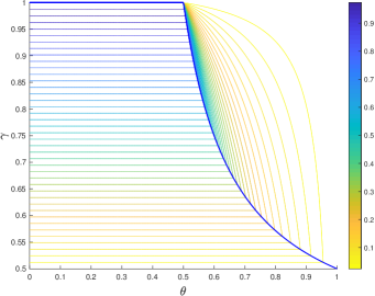
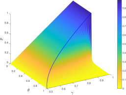
Figure 1: Contour and surface plot of the rates $\mathcal{O}(t^{-p})$ obtained in Theorem 3.16 as a multifunction of the step size parameter $\gamma\in(\frac{1}{2},1]$ and the KL exponent $\theta\in[0,1)$. The blue (transition) line depicts the rate along the set $\{(\theta,1):\theta\in[0,\frac{1}{2})\}\cup\{(\theta,\gamma):\theta=\gamma/(3\gamma-1)\}$.

3.5 Extension to Almost Sure Results

As we have mentioned, RR naturally is a stochastic optimization algorithm. Thus, it is paramount to generalize the convergence results derived for a single trajectory and to discuss convergence in a more rigorous stochastic framework. Fortunately, many of our results do not depend on the specific choice of the random permutations $\{\sigma^{t}\}_{t\geq 1}$ and can be easily transferred to the fully stochastic setting.

In the following, we briefly specify the underlying stochastic model for RR which allows us to describe the stochastic components of Algorithm 1 in a unified way. Based on the structure of Algorithm 1, we can define a suitable sample space $\Omega$ via $\Omega:=\Lambda^{\infty}:=\{\omega=(\omega_{1},\omega_{2},\omega_{3},\dots):\omega_{i}\in\Lambda\,\text{for all}\,i\}$, where $\Lambda$ is defined in (2). Each sample $\omega\in\Omega$ then corresponds to a specific sequence of (randomly chosen) permutations as generated, e.g., by a single run of Algorithm 1. Similar to infinite coin toss models, this sample space can be naturally equipped with a $\sigma$-algebra $\mathcal{F}$ and a probability function $\mathbb{P}$ to form a proper probability space $(\Omega,\mathcal{F},\mathbb{P})$.

Given this stochastic model, let us now consider a general stochastic process of iterates $\{X^{t}\}_{t\geq 1}$ generated by RR. So far the previous analysis was concerned with the investigation of a single trajectory $\{X^{t}(\omega)\}_{t\geq 1}\equiv\{x^{t}\}_{t\geq 1}$ for some fixed $\omega\in\Omega$. Since the proof of Proposition 3.5 is purely deterministic, we can immediately infer:

• Under assumption (A.1) and the step size condition (15), the stochastic process $\{f(X^{t})\}_{t\geq 1}$ surely converges to some random variable $F^{*}:\Omega\to\mathbb{R}$ and we have $\lim_{t\to\infty}\|\nabla f(X^{t})\|=0$ surely (i.e., for all $\omega\in\Omega$).

Generalizing the KL inequality-based results derived in Section 3.2 requires some more subtle changes. In particular, the set of accumulation points $\mathcal{C}$ defined in (9) depends on the selected sample $\omega\in\Omega$ and the trajectories of $\{X^{t}\}_{t\geq 1}$ might generally converge to different limit points. Hence, we need to work with proper stochastic extensions of the KL conditions formulated in Eq. 9. Let us first formally introduce the set of accumulation points $\mathcal{C}$ of $\{X^{t}\}_{t\geq 1}$ as the set-valued multifunction

$$\mathcal{C}:\Omega\rightrightarrows\mathbb{R}^{n},\quad\mathcal{C}(\omega):=\{x\in\mathbb{R}^{n}:\exists~{}\text{a subsequence}\;\{t_{\ell}\}_{\ell}\;\text{s.t.}\;X^{t_{\ell}}(\omega)\to x\text{ as }\ell\to\infty\}.$$

We can then consider the following stochastic versions of condition (B.1) and (B.3).

We assume the following conditions:

1. The stochastic process $\{X^{t}\}_{t\geq 1}$ is bounded almost surely, i.e., $\sup_{t}\|X^{t}\|<\infty$ almost surely.

2. There exists an event $\mathcal{K}\in\mathcal{F}$ with $\mathbb{P}(\mathcal{K})=1$ such that the KL inequality holds for every $\bar{x}\in\bigcup_{\omega\in\mathcal{K}}\mathcal{C}(\omega)$ and each respective desingularizing function $\varrho$ can be selected from the class of Łojasiewicz functions $\mathcal{L}$.

Notice that assumption (C.2) still holds if $f$ is subanalytic or semialgebraic. Furthermore, since the sequence $\{f(X^{t})\}_{t\geq 1}$ converges surely to some $F^{*}$, condition (C.1) is satisfied when $f$ is coercive or when it has bounded level sets. Under (C.1) and (C.2), we can now derive an almost sure variant of the convergence results established in Corollary 3.13 and Theorem 3.16.

Theorem 3.18.

Suppose that the assumptions (A.1), (C.1), and (C.2) are satisfied and let the step sizes $\{\alpha_{t}\}_{t\geq 1}$ be defined as in (36) for suitable choices of the parameters $\alpha$, $\beta$, and $\gamma$. Then, the stochastic process $\{X^{t}\}_{t\geq 1}$ almost surely converges to a $\mathrm{crit}(f)$-valued random vector $X^{*}:\Omega\to\mathrm{crit}(f)$. Furthermore, let $\Theta:\Omega\to[0,1)$ denote the function that maps each sample $\omega\in\mathcal{K}$ to the KL exponent of $f$ at $X^{*}(\omega)$ and let $C:\Omega\to\mathbb{R}_{+}$ be the corresponding function of KL constants. Then, the event

$$\mathcal{G}:=\left\{\omega\in\Omega:{\limsup}_{t\to\infty}\;t^{\Psi(\omega)}\cdot\|X^{t}(\omega)-X^{*}(\omega)\|<\infty\right\}$$

occurs almost surely, where the rate function $\Psi:\Omega\to\mathbb{R}_{+}$ is given by

(44) $$\Psi(\omega):=\begin{cases}2\gamma-1&\text{if }0\leq\Theta(\omega)<\frac{\gamma}{3\gamma-1}\;\text{and}\;\gamma\in(\frac{1}{2},1),\\ \frac{(1-\Theta(\omega))(1-\gamma)}{2\Theta(\omega)-1}&\text{if }\frac{\gamma}{3\gamma-1}\leq\Theta(\omega)<1\;\text{and}\;\gamma\in(\frac{1}{2},1),\\ 1&\text{if }\Theta(\omega)\in[0,\frac{1}{2}],\;\gamma=1,\;\text{and}\;{\alpha>\frac{8C^{2}(\omega)}{N}},\\ 0&\text{otherwise.}\end{cases}$$

Proof 3.19.

Assumptions (C.1) and (C.2) imply that there is an event $\mathcal{E}\in\mathcal{F}$ with $\mathbb{P}(\mathcal{E})=1$ such that $\{X^{t}(\omega)\}_{t\geq 1}$ is bounded for all $\omega\in\mathcal{E}$ and the Łojasiewicz inequality holds for every $\bar{x}\in\mathcal{C}(\omega)$ and all $\omega\in\mathcal{E}$. Hence, the results in Corollary 3.13 and Theorem 3.16 can be applied to all trajectories $\{X^{t}(\omega)\}_{t\geq 1}$, $\omega\in\mathcal{E}$ and we can infer $\mathcal{E}\subseteq\mathcal{G}$, which proves Theorem 3.18.

4 An Informal Analysis Framework and Reshuffled Proximal Point Method

In Section 3, we established the strong limit-point convergence results for RR under the KL inequality. One remarkable feature of our results is that RR is a non-descent method and the existing standard KL analysis framework is not applicable. In this section, we summarize the main steps and core ideas in an analysis framework. As an immediate application of such a framework, we show that the reshuffled proximal point method also shares the same convergence results as those of RR.

4.1 An Informal Analysis Framework

We consider the general problem

$$\operatorname*{\text{minimize}}_{x\in\mathbb{R}^{n}}\ f(x),$$

where the function $f:\mathbb{R}^{n}\rightarrow\mathbb{R}$ is smooth and bounded from below. In order to solve this problem, suppose we further have access to a generic (non-descent) algorithm $\cal A$ with diminishing step sizes $\{\alpha_{t}\}_{t\geq 1}$, which iterates as

$$x^{t}=\mathcal{A}(x^{t-1},\alpha_{t}),\quad t=1,2,\ldots$$

Typical requirements on the diminishing step sizes are

$$\alpha_{t}>0,\quad{\sum}_{t=1}^{\infty}\alpha_{t}=\infty,\quad\text{and}\quad{\sum}_{t=1}^{\infty}\alpha_{t}^{p}<\infty$$

for some $p\geq 2$. The goal is to establish strong limit-point convergence and derive the corresponding rate of convergence for algorithm $\mathcal{A}$. Our analysis in Section 3 consists of three main steps, which we summarize below in a simplified framework. For ease of exposition, we consider fixed permutations $\{\sigma^{t}\}_{t\geq 1}$ without randomness.

1. Approximate descent property. Based on the algorithmic properties of $\mathcal{A}$, show that

   $$f({x}^{t})\leq f({x}^{t-1})-\kappa_{1}\alpha_{t}\|\nabla{f}({x}^{t-1})\|^{2}-\frac{\kappa_{2}}{\alpha_{t}}\|{x}^{t}-{x}^{t-1}\|^{2}+\kappa_{3}\alpha_{t}^{q},$$

   where $\kappa_{1},\kappa_{3}>0$, $\kappa_{2}\geq 0$ and $q\geq p\geq 2$ are some constants.

2. Weak convergence. Based on the approximate descent property (A), establish weak convergence of $\mathcal{A}$, i.e., $\lim_{t\to\infty}\|\nabla f(x^{t})\|=0$. Consequently, any accumulation point of $\{x^{t}\}_{t\geq 1}$ is guaranteed to be a stationary point of $f$.

As mentioned, the sufficient decrease property is a ubiquitous ingredient of the standard KL analysis framework. With the help of this algorithmic property, it is quite straightforward to establish the weak convergence result formulated in (B); see, e.g., [14, Section 3.2]. However, due to the potential non-descent nature of the algorithmic scheme $\mathcal{A}$, it is unlikely to find such a sufficient decrease condition for $\mathcal{A}$ in general. Instead, based on the approximate descent property in (A), a more elementary analysis can be applied to prove weak convergence results via properly invoking the diminishing step sizes. Such a strategy allows to avoid the typical sufficient decrease condition.

Upon showing the weak convergence result, it is possible to infer several standard conclusions about the set of accumulation points and to derive a uniformized version of the KL inequality.

If $f$ further satisfies the KL inequality, then one can perform the last step:

1. Application of the KL inequality. Based on the KL inequality of $f$, verify that the whole sequence $\{x^{t}\}_{t\geq 1}$ converges to a single stationary point of $f$ and derive the corresponding convergence rates depending on the KL exponent $\theta$ and step size strategy.

One core idea is to derive an auxiliary descent-type condition for $\{x^{t}\}_{t\geq 1}$ by accumulating the potential ascent (i.e., the non-descent terms $\kappa_{3}\alpha_{t}^{q}$) in the approximate descent property of each step of the algorithm $\mathcal{A}$. Furthermore, the usage of the slightly stronger variant of the KL inequality in Definition 2.1, (B.2), or (B.3) allows to overcome the difficulties caused by the non-descent nature of $\{f(x^{t})\}_{t\geq 1}$. By combining the standard KL analysis framework and the dynamics of the diminishing step sizes one can then derive strong limit-point convergence and the corresponding convergence rates depending on the KL exponent $\theta$ and chosen step sizes.

Theorem 3.10 implies that strong limit-point convergence is typically a consequence of the finite length property of $\{x^{t}\}_{t\geq 1}$, i.e., $\kappa_{2}\sum_{t}\|x^{t}-x^{t-1}\|<\infty$. However, the property (A) allows the choice $\kappa_{2}=0$. In this case, one can still establish $\sum_{t}\alpha_{t}\|\nabla f(x^{t-1})\|<\infty$ as shown in the proof of Theorem 3.10. One possible way to prove strong limit-point convergence in this situation is to show a bound of the form $\|x^{t}-x^{t-1}\|\leq c_{1}\alpha_{t}\|\nabla f(x^{t-1})\|+c_{2}\alpha_{t}^{\bar{p}}$ with $\bar{p}\geq p$ and $c_{1},c_{2}>0$. Such a bound can be mild for a large class of non-descent methods [9]. Strong convergence can then be obtained by further invoking the conditions on the diminishing step sizes.

In principle, the above systematic strategy can be applied to non-descent methods that possess the approximate descent property (A). One example is RR, as verified in Lemma 3.3. In the next subsection, we introduce another algorithm that also satisfies this approximate descent property, and hence it has the same strong limit-point convergence results shown in Section 3 as well.

4.2 Reshuffled Proximal Point Method and its Convergence

As an application of the systematic framework stated in the last subsection, we consider another non-descent method—namely, the reshuffled proximal point method (RPP)—and establish its strong limit-point convergence result under the KL inequality.

RPP has the same algorithmic framework as RR (Algorithm 1) except for the updating step (3). RPP replaces (3) with the following proximal point step:

(45) $$\tilde{x}_{i}^{t}\in\operatorname*{argmin}_{x\in\mathbb{R}^{n}}\ f(x,\sigma^{t}_{i})+\frac{1}{2\alpha_{t}}\|x-\tilde{x}_{i-1}^{t}\|^{2}.$$

RPP covers the incremental proximal point method (cf. [7]) as a special case. Let us first interpret the update (45) as a certain gradient-type step. The first-order optimality condition underlying $\tilde{x}^{t}_{i}$ implies that

(46) $$\tilde{x}_{i}^{t}=\tilde{x}_{i-1}^{t}-\alpha_{t}\nabla f(\tilde{x}_{i}^{t},\sigma^{t}_{i}).$$

Clearly, this formula is similar to the update of RR. The only difference is that the gradient in (46) is evaluated implicitly at $\tilde{x}_{i}^{t}$, while the gradient in RR is evaluated at $\tilde{x}_{i-1}^{t}$. This observation motivates us to follow similar arguments to those of Lemma 3.1 and Lemma 3.3 for showing the approximate descent property of RPP.

Lemma 4.1.

Suppose that assumption (A.1) is valid. Let $\{x^{t}\}_{t\geq 1}$ be the sequence generated by RPP for solving problem (1) with step sizes $\{\alpha_{t}\}_{t\geq 1}$ satisfying $\alpha_{t}\in(0,{1}/{(\sqrt{2}{\sf L}N)}]$ and $\sum_{t=1}^{\infty}\alpha_{t}^{3}<\infty$. Then, for all $t\geq 1$, we have

(47) $$f(x^{t})\leq f(x^{t-1})-\frac{N\alpha_{t}}{2}\|\nabla{f}(x^{t-1})\|^{2}-\frac{1-{\sf L}N\alpha_{t}}{2N\alpha_{t}}\left\|x^{t}-x^{t-1}\right\|^{2}+2{\sf G}{\sf L}^{3}N^{3}\alpha_{t}^{3}.$$

Here, ${\sf G}:=\left(f(x^{0})-\bar{f}_{\min}\right)\exp\left(\sum_{j=1}^{\infty}6{\sf L}^{3}N^{3}\alpha_{j}^{3}\right)$ is a finite positive constant.

As the proof of Lemma 4.1 is essentially identical to our derivation of Lemma 3.3, we will omit details here. Lemma 4.1 characterizes the approximate descent property of RPP. Indeed, the recursion is the same as that of RR. Therefore, we can follow our analysis framework (A)–(C) to show similar strong limit-point convergence results to that of RR for RPP, which we summarize in the following corollary.

Corollary 4.2.

Suppose that the conditions (A.1), (C.1), and (C.2) are satisfied and let the stochastic process $\{X^{t}\}_{t\geq 1}$ be generated by RPP utilizing step sizes of the form (36). Then, $\{X^{t}\}_{t\geq 1}$ almost surely converges to a $\mathrm{crit}(f)$-valued random vector $X^{*}:\Omega\to\mathrm{crit}(f)$. Furthermore, let $\Theta:\Omega\to[0,1)$ denote the function that maps each sample $\omega\in\mathcal{K}$ to the KL exponent of $f$ at $X^{*}(\omega)$ and let $C:\Omega\to\mathbb{R}_{+}$ be the associated function of KL constants. Then, the event

$$\mathcal{H}:=\left\{\omega\in\Omega:{\limsup}_{t\to\infty}\;t^{\Psi(\omega)}\cdot\|X^{t}(\omega)-X^{*}(\omega)\|<\infty\right\}$$

occurs almost surely, where the rate function $\Psi:\Omega\to\mathbb{R}_{+}$ is given as in (44).

5 Conclusion

In this paper, we studied RR for smooth nonconvex optimization problems with a finite-sum structure. RR is a practical algorithm and widely utilized. Different from the existing convergence results for RR, we established the first strong limit-point convergence results for RR with appropriate diminishing step sizes under the KL inequality. In addition, we derived the corresponding rate of convergence, depending on the KL exponent $\theta$ and on suitably selected diminishing step sizes $\{\alpha_{t}\}_{t\geq 1}$. When $\theta\in[0,\frac{1}{2}]$, RR can achieve a rate of $\mathcal{O}(t^{-1})$. When $\theta\in(\frac{1}{2},1)$, RR has a convergence rate of the form $\mathcal{O}(t^{-q})$ with $q\in(0,1)$. Our results generalize the existing works that assume strong convexity to much broader nonconvex settings.

Our results motivated a new KL analysis framework, which generalizes the standard one to cover a class of non-descent methods with diminishing step sizes. We summarized the main ingredients of our derivations in an informal analysis framework, which is of independent interest. This more general KL framework can potentially be applied to various other non-descent methods with diminishing step sizes.

Appendix A Proof of Lemma 3.9

Proof A.1.

The first steps of the proof are identical to the derivation of [14, Lemma 6]. In particular, following the proof of [14, Lemma 6] and using Lemma 3.7, we can define a desingularizing function $\varrho\in\mathcal{S}_{\eta}$ of the form $\varrho(x):=\sum_{i=1}^{m}\varrho_{i}(x)$, $\varrho_{i}\in\mathcal{Q}_{\eta}$, $i=1,\dots,m$ that satisfies the uniformized KL inequality (22) for some $\delta,\eta,m>0$. The proof is complete if we can show $\varrho\in\mathcal{Q}_{\eta}$. Let $C_{\rho_{i}}>0$ denote the quasi-additivity constant in (5) associated with each $\varrho_{i}$, $i=1,\dots,m$, and let $x,y\in(0,\eta)$ with $x+y<\eta$ be arbitrary. Without loss of generality, let us assume $x\leq y$. Then, the concavity of $\varrho_{i}$ implies $\varrho_{i}^{\prime}(x)\geq\varrho_{i}^{\prime}(y)$ for all $i\in\{1,\dots,m\}$. In addition, let $j\in\{1,\dots,m\}$ be given with $\varrho_{j}^{\prime}(y)=\max_{1\leq i\leq m}\varrho_{i}^{\prime}(y)$. Using $\varrho_{i}^{\prime}(t)>0$ for all $t\in(0,\eta)$, $i\in\{1,\dots,m\}$, and (5) for $\varrho_{j}$, we obtain

$$\frac{1}{\varrho^{\prime}(x+y)} =\frac{1}{\varrho^{\prime}_{j}(x+y)+\sum_{i\neq j}\varrho^{\prime}_{i}(x+y)}\leq\frac{1}{\varrho^{\prime}_{j}(x+y)}\leq C_{\rho_{j}}\left[\frac{1}{\varrho_{j}^{\prime}(x)}+\frac{1}{\varrho_{j}^{\prime}(y)}\right]$$

$$\leq\frac{2C_{\rho_{j}}}{\varrho^{\prime}_{j}(y)}\leq\frac{2mC_{\rho_{j}}}{\varrho^{\prime}(y)}\leq 2m\max_{1\leq i\leq m}C_{\rho_{i}}\left[\frac{1}{\varrho^{\prime}(x)}+\frac{1}{\varrho^{\prime}(y)}\right].$$

Thus, $\varrho$ satisfies condition (5) with $C_{\rho}:=2m\max_{1\leq i\leq m}C_{\rho_{i}}$ and we have $\varrho\in\mathcal{Q}_{\eta}$.

Appendix B Proof of Lemma 3.12

Proof B.1.

We first note that the improper integral $\int_{t}^{\infty}\frac{\alpha^{3}}{(y+\beta)^{3\gamma}}\,\mathrm{d}y$ is finite. By the integral comparison test, we have $\sum_{j=t}^{\infty}\alpha_{j}^{3}\leq\alpha_{t}^{3}+\int_{t}^{\infty}\frac{\alpha^{3}}{(y+\beta)^{3\gamma}}\,\mathrm{d}y=\alpha_{t}^{3}+\frac{\alpha^{3}}{3\gamma-1}\frac{1}{(t+\beta)^{3\gamma-1}}$ and $\sum_{j=t}^{\infty}\alpha_{j}^{3}\geq\int_{t}^{\infty}\frac{\alpha^{3}}{(y+\beta)^{3\gamma}}\,\mathrm{d}y=\frac{\alpha^{3}}{3\gamma-1}\frac{1}{(t+\beta)^{3\gamma-1}}$. Using the monotonicity and subadditivity of the mapping $x\mapsto x^{\theta}$ and the bounds on $\sum_{j=t}^{\infty}\alpha_{j}^{3}$, we can infer $\frac{a_{\theta}}{(t+\beta)^{(3\gamma-1)\theta}}\leq[{\sum}_{j=t}^{\infty}\alpha_{j}^{3}]^{\theta}\leq\alpha^{3\theta}_{t}+\frac{a_{\theta}}{(t+\beta)^{(3\gamma-1)\theta}},$ where $a_{\theta}:=\alpha^{3\theta}/(3\gamma-1)^{\theta}$. Thus, we obtain

$$\sum_{t=k}^{\infty}\frac{a_{\theta}\alpha}{(t+\beta)^{(3\gamma-1)\theta+\gamma}}\leq\sum_{t=k}^{\infty}\alpha_{t}\left[{\sum}_{j=t}^{\infty}\alpha_{j}^{3}\right]^{\theta}\leq\sum_{t=k}^{\infty}\alpha_{t}^{1+3\theta}+\sum_{t=k}^{\infty}\frac{a_{\theta}\alpha}{(t+\beta)^{(3\gamma-1)\theta+\gamma}}.$$

Setting $\nu:=(1+3\theta)\gamma-(1+\theta)$, we can utilize the integral comparison test again to derive $\sum_{t=k}^{\infty}\alpha_{t}^{3\theta+1}\leq\alpha_{k}^{1+3\theta}+\int_{k}^{\infty}\frac{\alpha^{1+3\theta}}{(y+\beta)^{(1+3\theta)\gamma}}\,\mathrm{d}y=\alpha_{k}^{1+3\theta}+\frac{k+\beta}{(1+3\theta)\gamma-1}\cdot\alpha_{k}^{1+3\theta}$ and $\frac{\nu^{-1}}{(k+\beta)^{\nu}}\leq\sum_{t=k}^{\infty}\frac{1}{(t+\beta)^{(3\gamma-1)\theta+\gamma}}\leq\frac{1}{(k+\beta)^{(3\gamma-1)\theta+\gamma}}+\frac{\nu^{-1}}{(k+\beta)^{\nu}}$. Plugging these bounds into the estimate for $\sum_{t=k}^{\infty}\alpha_{t}[{\sum}_{j=t}^{\infty}\alpha_{j}^{3}]^{\theta}$, it follows

$$\frac{a_{\theta}\alpha\nu^{-1}}{(k+\beta)^{\nu}}\leq{\sum}_{t=k}^{\infty}\alpha_{t}\left[{\sum}_{j=t}^{\infty}\alpha_{j}^{3}\right]^{\theta}$$

$$\leq\left[\alpha_{k}^{1+3\theta}+\frac{k+\beta}{(1+3\theta)\gamma-1}\cdot\alpha_{k}^{1+3\theta}\right]+\frac{a_{\theta}\alpha}{(k+\beta)^{(3\gamma-1)\theta+\gamma}}+\frac{a_{\theta}\alpha\nu^{-1}}{(k+\beta)^{\nu}}$$

$$=\left\{a_{\theta}\left[\frac{\alpha}{k+\beta}+\frac{\alpha}{\nu}\right]+\left[\frac{\alpha^{1+3\theta}}{(k+\beta)^{1+\theta}}+\frac{\alpha^{1+3\theta}}{(\gamma+3\theta\gamma-1)(k+\beta)^{\theta}}\right]\right\}\cdot\frac{1}{(k+\beta)^{\nu}}$$

$$\leq\bar{a}_{\theta}\cdot\frac{1}{(k+\beta)^{\nu}}.$$

where $\bar{a}_{\theta}:=\frac{a_{\theta}\alpha}{1+\beta}+\frac{a_{\theta}\alpha}{\nu}+\frac{\alpha^{1+3\theta}}{(1+\beta)^{1+\theta}}+\frac{\alpha^{1+3\theta}}{(\gamma+3\theta\gamma-1)(1+\beta)^{\theta}}$. In summary, this yields

$$\frac{\underline{a}_{\theta}}{(k+\beta)^{(1+3\theta)\gamma-(1+\theta)}}\leq{\sum}_{t=k}^{\infty}\alpha_{t}\left[{\sum}_{j=t}^{\infty}\alpha_{j}^{3}\right]^{\theta}\leq\frac{\bar{a}_{\theta}}{(k+\beta)^{(1+3\theta)\gamma-(1+\theta)}},$$

where $\underline{a}_{\theta}:=a_{\theta}\alpha[(1+3\theta)\gamma-(1+\theta)]^{-1}$.

Appendix C The Supermartingale Convergence Theorem

We present the supermartingale convergence theorem [8, Proposition A.31] below for convenience.

Lemma C.1.

Let $\{y_{k}\}_{k\geq 1},\{z_{k}\}_{k\geq 1},\{w_{k}\}_{k\geq 1}$, and $\{v_{k}\}_{k\geq 1}$ be sequences such that

$$y_{k+1}\leq(1+v_{k})y_{k}-z_{k}+w_{k},\quad k=1,2,\dots,$$

$\{z_{k}\}_{k\geq 1},\{w_{k}\}_{k\geq 1}$ and $\{v_{k}\}_{k\geq 1}$ are nonnegative, and

$${\sum}_{k=1}^{\infty}w_{k}<\infty,\quad{\sum}_{k=1}^{\infty}v_{k}<\infty.$$

Then, either $y_{k}\to-\infty$, or else $\{y_{k}\}_{k\geq 1}$ converges to a finite value and ${\sum}_{k=1}^{\infty}z_{k}<\infty$.

References

- [1] M. Abadi, A. Agarwal, P. Barham, E. Brevdo, Z. Chen, C. Citro, G. S. Corrado, A. Davis, et al., TensorFlow: Large-scale machine learning on heterogeneous systems, 2015.
- [2] P.-A. Absil, R. Mahony, and B. Andrews, Convergence of the iterates of descent methods for analytic cost functions, SIAM J. Optim., 16 (2005), pp. 531–547.
- [3] A. Agarwal, P. L. Bartlett, P. Ravikumar, and M. J. Wainwright, Information-theoretic lower bounds on the oracle complexity of stochastic convex optimization, IEEE Trans. Inf. Theory, 58 (2012), pp. 3235–3249.
- [4] H. Attouch and J. Bolte, On the convergence of the proximal algorithm for nonsmooth functions involving analytic features, Math. Program., 116 (2009), pp. 5–16.
- [5] H. Attouch, J. Bolte, P. Redont, and A. Soubeyran, Proximal alternating minimization and projection methods for nonconvex problems: an approach based on the Kurdyka-Łojasiewicz inequality, Math. Oper. Res., 35 (2010), pp. 438–457.
- [6] H. Attouch, J. Bolte, and B. F. Svaiter, Convergence of descent methods for semi-algebraic and tame problems: proximal algorithms, forward-backward splitting, and regularized Gauss-Seidel methods, Math. Program., 137 (2013), pp. 91–129.
- [7] D. P. Bertsekas, Incremental proximal methods for large scale convex optimization, Math. Program., 129 (2011), p. 163.
- [8] D. P. Bertsekas, Nonlinear programming, Athena Scientific Optimization and Computation Series, Athena Scientific, Belmont, MA, third ed., 2016.
- [9] D. P. Bertsekas and J. N. Tsitsiklis, Gradient convergence in gradient methods with errors, SIAM J. Optim., 10 (2000), pp. 627–642.
- [10] J. Bolte, A. Daniilidis, and A. Lewis, The Łojasiewicz inequality for nonsmooth subanalytic functions with applications to subgradient dynamical systems, SIAM J. Optim., 17 (2006), pp. 1205–1223.
- [11] J. Bolte, A. Daniilidis, and A. Lewis, A nonsmooth Morse-Sard theorem for subanalytic functions, J. Math. Anal. Appl., 321 (2006), pp. 729–740.
- [12] J. Bolte, A. Daniilidis, A. Lewis, and M. Shiota, Clarke subgradients of stratifiable functions, SIAM J. Optim., 18 (2007), pp. 556–572.
- [13] J. Bolte, A. Daniilidis, O. Ley, and L. Mazet, Characterizations of Łojasiewicz inequalities: subgradient flows, talweg, convexity, Trans. Amer. Math. Soc., 362 (2010), pp. 3319–3363.
- [14] J. Bolte, S. Sabach, and M. Teboulle, Proximal alternating linearized minimization for nonconvex and nonsmooth problems, Math. Program., 146 (2014), pp. 459–494.
- [15] R. I. Boţ, E. R. Csetnek, and S. C. László, An inertial forward–backward algorithm for the minimization of the sum of two nonconvex functions, EURO J. Comput. Optim., 4 (2016), pp. 3–25.
- [16] R. I. Boţ and D.-K. Nguyen, The proximal alternating direction method of multipliers in the nonconvex setting: convergence analysis and rates, Math. Oper. Res., 45 (2020), pp. 682–712.
- [17] L. Bottou, Curiously fast convergence of some stochastic gradient descent algorithms, in Proceedings of the Symposium on Learning and Data Science, Paris, 2009.
- [18] L. Bottou, Stochastic gradient descent tricks, in Neural Networks: Tricks of the Trade, Springer, 2012, pp. 421–436.
- [19] L. Bottou, F. E. Curtis, and J. Nocedal, Optimization methods for large-scale machine learning, SIAM Review, 60 (2018), pp. 223–311.
- [20] Y. Chi, Y. M. Lu, and Y. Chen, Nonconvex optimization meets low-rank matrix factorization: An overview, IEEE Transactions on Signal Processing, 67 (2019), pp. 5239–5269.
- [21] K. L. Chung, On a stochastic approximation method, The Annals of Mathematical Statistics, (1954), pp. 463–483.
- [22] A. R. Conn, N. I. Gould, and P. L. Toint, Trust region methods, SIAM, 2000.
- [23] P. Frankel, G. Garrigos, and J. Peypouquet, Splitting methods with variable metric for Kurdyka–Łojasiewicz functions and general convergence rates, Journal of Optimization Theory and Applications, 165 (2015), pp. 874–900.
- [24] G. Garrigos, Descent dynamical systems and algorithms for tame optimization, and multi-objective problems, PhD thesis, Université Montpellier; Universidad técnica Federico Santa María (Valparaiso, Chili), 2015.
- [25] M. Gürbüzbalaban, A. Ozdaglar, and P. Parrilo, Why random reshuffling beats stochastic gradient descent, Math. Program., 186 (2021), pp. 49–84.
- [26] M. Gürbüzbalaban, A. Ozdaglar, and P. A. Parrilo, Convergence rate of incremental gradient and incremental Newton methods, SIAM J. Optim., 29 (2019), pp. 2542–2565.
- [27] J. Z. HaoChen and S. Sra, Random shuffling beats SGD after finite epochs, in International Conference on Machine Learning, 2019, pp. 2624–2633.
- [28] Y. Hu, J. Li, and C. K. W. Yu, Convergence rates of subgradient methods for quasi-convex optimization problems, Comput. Optim. Appl., 77 (2020), pp. 183–212.
- [29] X. Huang, K. Yuan, X. Mao, and W. Yin, An improved analysis and rates for variance reduction under without-replacement sampling orders, Advances in Neural Information Processing Systems, 34 (2021).
- [30] K. Kurdyka, On gradients of functions definable in o-minimal structures, Annales de l’Institut Fourier, 48 (1998), pp. 769–783.
- [31] K. Kurdyka and A. Parusinski, -stratification of subanalytic functions and the Łojasiewicz inequality, Comptes rendus de l’Académie des sciences. Série 1, Mathématique, 318 (1994), pp. 129–133.
- [32] Z. Lai and L.-H. Lim, Recht-ré noncommutative arithmetic-geometric mean conjecture is false, in International Conference on Machine Learning, PMLR, 2020, pp. 5608–5617.
- [33] G. Li and T. K. Pong, Global convergence of splitting methods for nonconvex composite optimization, SIAM J. Optim., 25 (2015), pp. 2434–2460.
- [34] G. Li and T. K. Pong, Douglas–Rachford splitting for nonconvex optimization with application to nonconvex feasibility problems, Math. Program., 159 (2016), pp. 371–401.
- [35] S. Łojasiewicz, Sur le problème de la division, Studia Mathematica, 18 (1959), pp. 87–136.
- [36] S. Łojasiewicz, Une propriété topologique des sous-ensembles analytiques réels, Les équations aux dérivées partielles, 117 (1963), pp. 87–89.
- [37] S. Łojasiewicz, Sur la géométrie semi- et sous-analytique, Annales de l’institut Fourier (Grenoble), 43 (1993), pp. 1575–1595.
- [38] Z.-Q. Luo and P. Tseng, Analysis of an approximate gradient projection method with applications to the backpropagation algorithm, Optim. Method Softw., 4 (1994), pp. 85–101.
- [39] K. Mishchenko, A. Khaled, and P. Richtárik, Random reshuffling: Simple analysis with vast improvements, Advances in Neural Information Processing Systems, 33 (2020).
- [40] D. Nagaraj, J. Prateek, and N. Praneeth, SGD without replacement: Sharper rates for general smooth convex functions, in International Conference on Machine Learning, 2019, pp. 4703–4711.
- [41] A. S. Nemirovskij and D. B. Yudin, Problem complexity and method efficiency in optimization, Wiley-Interscience Series in Discrete Mathematics, Wiley, Chichester, 1983.
- [42] Y. Nesterov, Introductory lectures on convex optimization: A basic course, vol. 87, Springer Science & Business Media, 2003.
- [43] L. M. Nguyen, Q. Tran-Dinh, D. T. Phan, P. H. Nguyen, and M. van Dijk, A unified convergence analysis for shuffling-type gradient methods, Journal of Machine Learning Research, (2021).
- [44] P. Ochs, Y. Chen, T. Brox, and T. Pock, iPiano: Inertial proximal algorithm for nonconvex optimization, SIAM J. Imaging Sci., 7 (2014), pp. 1388–1419.
- [45] A. Paszke, S. Gross, F. Massa, A. Lerer, J. Bradbury, G. Chanan, T. Killeen, Z. Lin, N. Gimelshein, L. Antiga, et al., Pytorch: An imperative style, high-performance deep learning library, Advances in neural information processing systems, 32 (2019).
- [46] T. Pock and S. Sabach, Inertial proximal alternating linearized minimization (iPALM) for nonconvex and nonsmooth problems, SIAM J. Imaging Sci., 9 (2016), pp. 1756–1787.
- [47] B. T. Polyak, Introduction to optimization, Translations Series in Mathematics and Engineering, Optimization Software, Inc., Publications Division, New York, 1987. Translated from the Russian, With a foreword by Dimitri P. Bertsekas.
- [48] B. Recht and C. Ré, Toward a noncommutative arithmetic-geometric mean inequality: conjectures, case-studies, and consequences, in Conference on Learning Theory, JMLR Workshop and Conference Proceedings, 2012, pp. 11–1.
- [49] H. Robbins and S. Monro, A stochastic approximation method, The annals of mathematical statistics, (1951), pp. 400–407.
- [50] O. Shamir, Without-replacement sampling for stochastic gradient methods, in Advances in Neural Information Processing Systems, 2016, pp. 46–54.
- [51] M. V. Solodov, Incremental gradient algorithms with stepsizes bounded away from zero, Comput. Optim. Appl., 11 (1998), pp. 23–35.
- [52] M. V. Solodov and S. Zavriev, Error stability properties of generalized gradient-type algorithms, J. Optim. Theory Appl., 98 (1998), pp. 663–680.
- [53] P. Tseng, An incremental gradient(-projection) method with momentum term and adaptive stepsize rule, SIAM J. Optim., 8 (1998), pp. 506–531.
- [54] Y. Wang, W. Yin, and J. Zeng, Global convergence of ADMM in nonconvex nonsmooth optimization, J. Sci. Comput., 78 (2019), pp. 29–63.