Tensor Arnoldi-Tikhonov and GMRES-type methods for ill-posed problems with a t-product structure

Abstract

This paper describes solution methods for linear discrete ill-posed problems defined by third order tensors and the t-product formalism introduced in [M. E. Kilmer and C. D. Martin, Factorization strategies for third order tensors, Linear Algebra Appl., 435 (2011), pp. 641–658]. A t-product Arnoldi (t-Arnoldi) process is defined and applied to reduce a large-scale Tikhonov regularization problem for third order tensors to a problem of small size. The data may be represented by a laterally oriented matrix or a third order tensor, and the regularization operator is a third order tensor. The discrepancy principle is used to determine the regularization parameter and the number of steps of the t-Arnoldi process. Numerical examples compare results for several solution methods, and illustrate the potential superiority of solution methods that tensorize over solution methods that matricize linear discrete ill-posed problems for third order tensors.

Key words: discrepancy principle, linear discrete ill-posed problem, tensor Arnoldi process, t-product, tensor Tikhonov regularization.

1 Introduction

We are concerned with the solution of large-scale least squares problems of the form

$$\min_{\mathcal{\vec{X}}\in\mathbb{R}^{m\times 1\times n}}\|\mathcal{A*\vec{X}-\vec{B}}\|_{F},$$ (1.1)

where $\mathcal{A}=[a_{ijk}]_{i,j,k=1}^{m,m,n}\in\mathbb{R}^{m\times m\times n}$ is a third order tensor of ill-determined tubal rank, i.e., the Frobenius norm of the singular tubes of $\mathcal{A}$, which are analogues of the singular values of a matrix, decay rapidly to zero with increasing index, and there are many nonvanishing singular tubes of tiny Frobenius norm of different orders of magnitude (cf. Definition 2.2 below). Least squares problems with a tensor of this kind are referred to as linear discrete ill-posed problems. The tensors $\mathcal{\vec{X}}\in\mathbb{R}^{m\times 1\times n}$ and $\mathcal{\vec{B}}\in\mathbb{R}^{m\times 1\times n}$ in (1.1) are lateral slices of third order tensors, and the operator $\ast$ denotes the tensor t-product introduced in the seminal work by Kilmer and Martin [24]. We will review the t-product in Section 2.

An advantage of the formulation (1.1) with the t-product, when compared to other products, is that the t-product avoids loss of information inherent in the flattening of a tensor; see Kilmer et al. [23]. The t-product preserves the natural ordering and higher correlations embedded in the data, and has been found useful in many application areas, including completion of seismic data [11], image deblurring problems [10, 23, 24, 36], facial recognition [19], tomographic image reconstruction [41], and tensor compression [43].

Throughout this paper, $\|\cdot\|_{F}$ denotes the Frobenius norm of a third order tensor, which for $\mathcal{A}=[a_{ijk}]_{i,j,k=1}^{m,m,n}\in\mathbb{R}^{m\times m\times n}$ is defined by

$$\|\mathcal{A}\|_{F}=\sqrt{\sum_{i=1}^{m}\sum_{j=1}^{m}\sum_{k=1}^{n}a^{2}_{ijk}}.$$

In applications of interest to us, such as image and video restoration, the data tensor $\mathcal{\vec{B}}\in\mathbb{R}^{m\times 1\times n}$ is contaminated by measurement error (noise) that is represented by a tensor $\mathcal{\vec{E}}\in\mathbb{R}^{m\times 1\times n}$. Thus,

$$\mathcal{\vec{B}}=\mathcal{\vec{B}}_{\text{true}}+\mathcal{\vec{E}},$$ (1.2)

where $\mathcal{\vec{B}}_{\text{true}}\in\mathbb{R}^{m\times 1\times n}$ represents the unavailable error-free data tensor that is associated with the known data tensor $\mathcal{\vec{B}}$. We assume the unavailable linear system of equations

$$\mathcal{A*\vec{X}=\vec{B}}_{\text{true}}$$

to be consistent and let $\mathcal{\vec{X}_{\text{true}}}$ denote its (unknown) exact solution of minimal Frobenius norm.

We would like to compute an accurate approximation of $\mathcal{\vec{X}_{\text{true}}}$. Straightforward solution of (1.1) typically does not yield a meaningful approximation of $\mathcal{\vec{X}}_{\text{true}}$, because the severe ill-conditioning of $\mathcal{A}$ and the error in $\mathcal{\vec{B}}$ result in a large propagated error in the computed solution. We remedy this difficulty by replacing (1.1) by a nearby problem that is less sensitive to perturbations of the right-hand side $\mathcal{\vec{B}}$, i.e., we solve the penalized least squares problem

$$\min_{\mathcal{\vec{X}}\in\mathbb{R}^{m\times 1\times n}}\left\{\|\mathcal{A*\vec{X}-\vec{B}}\|_{F}^{2}+\mu^{-1}\|\mathcal{L*\vec{X}}\|_{F}^{2}\right\},$$ (1.3)

where $\mathcal{L}\in\mathbb{R}^{s\times m\times n}$ is a regularization operator and $\mu>0$ is a regularization parameter. This replacement is commonly referred to as Tikhonov regularization. Let $\mathcal{N}(\mathcal{M})$ denote the null space of the tensor $\mathcal{M}$ under $*$ and assume that $\mathcal{L}$ satisfies

$$\mathcal{N}(\mathcal{A})\cap\mathcal{N}(\mathcal{L})=\{\mathcal{\vec{O}}\},$$ (1.4)

where $\mathcal{\vec{O}}$ denotes an $m\times n$ zero matrix oriented laterally; see below. Then (1.3) has a unique solution $\mathcal{\vec{X}}_{\mu}\in\mathbb{R}^{m\times 1\times n}$ for any $\mu>0$ (cf. Theorem 3.1). The closeness of $\mathcal{\vec{X}}_{\mu}$ to $\mathcal{\vec{X}}_{\text{true}}$ and the sensitivity of $\mathcal{\vec{X}}_{\mu}$ to the error $\mathcal{E}$ in $\mathcal{B}$ depends on the value of $\mu$. We determine $\mu$ by the discrepancy principle, which is described and analyzed in, e.g., [12]. Application of the discrepancy principle requires that a bound

$$\|\mathcal{\vec{E}}\|_{F}\leq\delta$$ (1.5)

be available. The parameter $\mu>0$ then is determined so that $\mathcal{\vec{X}}_{\mu}$ satisfies

$$\|\mathcal{\vec{B}}-\mathcal{A}*\mathcal{\vec{X}}_{\mu}\|_{F}=\eta\delta,$$ (1.6)

where $\eta>1$ is a user specified constant independent of $\delta>0$. It can be shown that $\mathcal{\vec{X}}_{\mu}\rightarrow\mathcal{\vec{X}}_{\text{true}}$ as $\delta\searrow 0$; see [12] for a proof in a Hilbert space setting.

Many other methods, including generalized cross validation (GCV) and the L-curve criterion, also can be used to determine the regularization parameter; see, e.g., [5, 13, 15, 16, 25, 26, 37] for discussions and illustrations for the situation when $\mathcal{A}$ is a matrix and $\mathcal{\vec{B}}$ is a vector.

It is well known that a few steps of the (standard) Arnoldi process can be used to reduce a large matrix to a matrix of small size. The small matrix so obtained can be used to define a small Tikhonov regularization problems that is easy to solve; see [5, 7, 14, 28] for discussions and illustrations. It is the purpose of the present paper to extend the (standard) matrix version of the Arnoldi process, described, e.g., in [38], to third order tensors using the t-product formalism. This gives us the t-Arnoldi process. Application of $\ell\geq 1$ steps of this process, generically, furnishes an orthonormal basis for the $\ell$-dimensional tensor Krylov (t-Krylov) subspace

$$\mathbb{K}_{\ell}(\mathcal{A},\mathcal{\vec{B}})={\rm\text{t-span}}\left\{\mathcal{\vec{B}},\mathcal{A}*\mathcal{\vec{B}},\mathcal{A}^{2}*\mathcal{\vec{B}},\dots,\mathcal{A}^{\ell-1}*\mathcal{\vec{B}}\right\}.$$ (1.7)

The meaning of t-span is discussed in Sections 3 and 4. Each step of the t-Arnoldi process requires one tensor-matrix product evaluation with $\mathcal{A}$. Often fewer tensor-matrix product evaluations are required to solve Tikhonov minimization problems (1.3) than when the t-product Golub-Kahan bidiagonalization (tGKB) process, described by Kilmer et al. [23] is used, because each step of the latter demands two tensor-matrix product evaluations, one with $\mathcal{A}$ and one with $\mathcal{A}^{T}$, where the superscript ^T denotes transposition.

We refer to our solution scheme for (1.3) as the t-product Arnoldi-Tikhonov (tAT) regularization method. It is based on reducing the tensor $\mathcal{A}\in\mathbb{R}^{m\times m\times n}$ to a small upper Hessenberg tensor. We also describe a global tAT (G-tAT) method for the solution of (1.3). This method works with a data tensor slice $\mathcal{\vec{B}}\in\mathbb{R}^{m\times 1\times n}$ and is closely related to the T-global Arnoldi-Tikhonov regularization method recently described by El Guide et al. [10], which takes $\mathcal{L}$ equal to the identity tensor denoted by $\mathcal{I}$, determines the regularization parameter by the GCV method, and works with a general data tensor $\mathcal{B}\in\mathbb{R}^{m\times p\times n}$, $p>1$. Differently from the tAT method, the G-tAT and the T-global Arnoldi-Tikhonov regularization methods involve matricization of the tensor $\mathcal{A}$. Specifically, the G-tAT method first reduces $\mathcal{A}$ in (1.3) to an upper Hessenberg matrix by carrying out a few steps of the global t-Arnoldi (G-tA) process. This process furnishes an orthonormal basis for a t-Krylov subspace (1.7). It differs from the t-Arnoldi process in the choice of inner product. Algorithm 13 in Section 5 provides the details of the G-tA process. Numerical examples with the t-Arnoldi and G-tA processes are presented in Section 6. The tAT and G-tAT methods based on these processes determine the regularization parameter by the discrepancy principle.

We also describe an extension of the (standard) generalized minimal residual (GMRES) method proposed by Saad and Schultz [39] to third order tensors based on the t-product formalism. This extension will be referred to as the t-product GMRES (tGMRES) method. The tGMRES method for the solution of (1.1) computes iterates in t-Krylov subspaces of the form (1.7); the $\ell$th approximate solution $\mathcal{\vec{X}}_{\ell}$ determined by tGMRES with initial approximate solution $\mathcal{\vec{X}}_{0}=\mathcal{\vec{O}}$ satisfies

$$\|\mathcal{A}*\mathcal{\vec{X}}_{\ell}-\mathcal{\vec{B}}\|_{F}=\min_{\mathcal{\vec{X}}\in\mathbb{K}_{\ell}(\mathcal{A},\mathcal{\vec{B}})}\|\mathcal{A*\vec{X}-\vec{B}}\|_{F},\;\;\;\ell=1,2,\dots~{}.$$ (1.8)

Another extension of the (standard) GMRES method by Saad and Schulz [39] for the solution of tensor equations is provided by the global tGMRES (G-tGMRES) method, which is described in Subsection 5.2. This method is closely related to the T-global GMRES method recently presented by El Guide et al. [10]. The methods differ in that the data for the G-tGMRES method is represented by a lateral slice $\mathcal{\vec{B}}$, while the data for T-global GMRES method is a general third order tensor $\mathcal{B}\in\mathbb{R}^{m\times p\times n}$, $p>1$. Moreover, our implementation of the t-GMRES and G-tGMRES methods uses the discrepancy principle to determine when to terminate the iterations. Differently from the tGMRES method, the G-tGMRES and T-global GMRES methods involve matricization of the tensor $\mathcal{A}$. While the tGMRES method is based on the t-Arnoldi process described in Section 3, the G-tGMRES method is based on the global t-Arnoldi (G-tA) process.

Many other methods for solving (1.3) and (1.8) that do not apply the t-product have been described in the literature; see, e.g., [2, 8, 9, 40]. These methods replace matrix-vector products by tensor-matrix products and involve matricization. A careful comparison of all these methods is outside the scope of the present paper. Here we note that computed examples of Section 6 indicate that methods that avoid matricization often determine approximate solutions of higher quality than methods that involve matricization.

We also are interested in solving minimization problems analogous to (1.1), in which $\mathcal{\vec{B}}$ is replaced by a general third order tensor $\mathcal{B}$. This leads to the Tikhonov minimization problem

$$\min_{\mathcal{X}\in\mathbb{R}^{m\times p\times n}}\left\{\|\mathcal{A}*\mathcal{X}-\mathcal{B}\|_{F}^{2}+\mu^{-1}\|\mathcal{L*X}\|_{F}^{2}\right\},\;\;\;\mathcal{B}\in\mathbb{R}^{m\times p\times n},\;\;\;p>1.$$ (1.9)

Besides our work [36], no literature is available on solution methods for (1.3) and (1.9) for $\mathcal{L\neq I}$. The present paper focuses on developing tensor Arnoldi-Tikhonov-type methods for this situation.

Four methods for the solution of (1.9) will be described. Three of them are based on the tAT and G-tAT methods applied to the lateral slices $\mathcal{\vec{B}}_{j}$, $j=1,2,\dots,p$, of $\mathcal{B}$, independently. The other method generalizes the T-global Arnoldi-Tikhonov regularization method recently presented by El Guide et al. [10] to allow for $\mathcal{L}\neq\mathcal{I}$. This method works with the lateral slices of the data tensor $\mathcal{B}$ simultaneously, and will be referred to as the generalized global tAT (GG-tAT) method.

A comparison of the solution methods for (1.9) is presented in Section 6. Computed examples show the GG-tAT method to require less CPU time, but the G-tAT method may yield higher accuracy. The fact that the GG-tAT requires less CPU time is to be expected since it uses larger chunks of data at a time.

We remark that the G-tAT and GG-tAT methods belong to the AT$\_$BTF (Arnoldi-Tikhonov Based Tensor Format) family of methods recently described by Beik et al. [2]. They involve flattening and require additional product definitions to the t-product.

Finally, we will discuss a variant of the T-global GMRES method that recently has been described by El Guide et al. [10] and is based on t-product formalism. We will refer to our variant as the generalized global tGMRES (GG-tGMRES) method. This method replaces the data tensor $\mathcal{\vec{B}}$ in (1.8) by a general third order tensor $\mathcal{B}$ and determines iterates in t-Krylov subspaces $\mathbb{K}_{\ell}(\mathcal{A},\mathcal{B})$. The $\ell$th iterate $\mathcal{X}_{\ell}$ determined by the GG-tGMRES method with initial iterate $\mathcal{X}_{0}=\mathcal{O}\in\mathbb{R}^{m\times p\times n}$ solves

$$\|\mathcal{A}*\mathcal{X}_{\ell}-\mathcal{B}\|_{F}=\min_{\mathcal{X}\in\mathbb{K}_{\ell}(\mathcal{A},\mathcal{B})}\|\mathcal{A*\mathcal{X}-\mathcal{B}}\|_{F},\;\;\;\ell=1,2,\dots~{}.$$ (1.10)

In the T-global GMRES method by El Guide et al. [10], the iterations are terminated based on a residual Frobenius norm and a set tolerance that is independent of the error in $\mathcal{B}$. Differently from the T-global GMRES method, our approach for solving (1.10) uses the discrepancy principle to determine the number of iterations to carry out with the GG-tGMRES method.

This paper is organized as follows. Section 2 introduces notation and preliminaries associated with the t-product. Methods based on the t-Arnoldi process are described in Section 3. This includes Tikhonov regularization methods, one of which is based on a nested t-Krylov subspace, and GMRES-type methods for the computation of approximate solutions of (1.1) and the analogous minimization problem obtained by replacing the tensor slice $\mathcal{\vec{B}}$ by a third order tensor $\mathcal{B}$. Thus, we can consider color image and video restoration problems. For the former, $\mathcal{B}$ represents a blurred and noisy RGB image of dimension $m\times p\times 3$, while for gray-scale video restoration problems, $\mathcal{B}$ is of dimension $m\times p\times n$ with a sequence of $n$ consecutive blurred and noisy video frames. Section 4 describes algorithms that are based on the generalized global t-Arnoldi (GG-tA) process with data tensor $\mathcal{B}$. The algorithms of Section 5 are obtained by modifying algorithms of Section 4 to be applicable to each lateral slice of $\mathcal{B}$ separately. This allows us to consider, for instance, the restoration of gray-scale images. Section 6 presents some numerical examples that illustrate the performance of these methods. Concluding remarks can be found in Section 7.

2 Notation and Preliminaries

This section reviews results on the t-product introduced by Kilmer et al. [23, 24] and defines notation from [24, 27] to be used in the sequel. In this paper, a tensor is of third order, i.e., a three-dimensional array of real scalars denoted by the calligraphic script letters, say, $\mathcal{A}=[a_{ijk}]_{i,j,k=1}^{\ell,m,n}\in\mathbb{R}^{\ell\times m\times n}$ with real entries $a_{ijk}$. Matrices and vectors are second and first order tensors, respectively. We use capital letters to denote matrices, lower case letters to denote vectors, and bold face lower case letters to denote tube fibers (tubal scalars or tubes). A fiber of a third order tensor is a 1D section obtained by fixing two of the indices. Using MATLAB notation, $\mathcal{A}(:,j,k)$, $\mathcal{A}(i,:,k)$, and $\mathcal{A}(i,j,:)$ denote mode-1, mode-2, and mode-3 fibers, respectively. A slice of a third order tensor is a 2D section obtained by fixing one of the indices. With MATLAB notation, $\mathcal{A}(i,:,:)$, $\mathcal{A}(:,j,:)$, and $\mathcal{A}(:,:,k)$ denote the $i$th horizontal, $j$th lateral, and $k$th frontal slices, respectively. The $j$th lateral slice is also denoted by $\mathcal{\vec{A}}_{j}$. It is a tensor and will be referred to as a tensor column. Moreover, the $k$th frontal slice, which also will be denoted by $\mathcal{A}^{(k)}$, is a matrix.

Given $\mathcal{A}\in\mathbb{R}^{\ell\times m\times n}$ with $\ell\times m$ frontal slices $\mathcal{A}^{(i)}$, $i=1,2,\dots,n$, the operator $\mathtt{unfold}(\mathcal{A})$ returns a block $\ell n\times m$ matrix made up of the faces $\mathcal{A}^{(i)}$ of $\mathcal{A}$. The $\mathtt{fold}$ operator folds back the unfolded $\mathcal{A}$, i.e.,

$$\mathtt{unfold}(\mathcal{A})=\begin{bmatrix}\mathcal{A}^{(1)}\\ \mathcal{A}^{(2)}\\ \vdots\\ \mathcal{A}^{(n)}\end{bmatrix},\;\;\;\;\;\mathtt{fold(unfold(\mathcal{A}))=\mathcal{A}}.$$

The operator $\mathtt{bcirc}(\mathcal{A})$ generates an $\ell n\times mn$ block circulant matrix with $\mathtt{unfold}(\mathcal{A})$ forming the first block column,

$$\mathtt{bcirc}(\mathcal{A})=\begin{bmatrix}\mathcal{A}^{(1)}&\mathcal{A}^{(n)}&\dots&\mathcal{A}^{(2)}\\ \mathcal{A}^{(2)}&\mathcal{A}^{(1)}&\dots&\mathcal{A}^{(3)}\\ \vdots&\vdots&\ddots&\vdots\\ \mathcal{A}^{(n)}&\mathcal{A}^{(n-1)}&\dots&\mathcal{A}^{(1)}\end{bmatrix}.$$

Definition 2.1.

(t-product [24]) Let $\mathcal{A}\in\mathbb{R}^{\ell\times m\times n}$ and $\mathcal{B}\in\mathbb{R}^{m\times p\times n}$. Then the t-product $\mathcal{A*B}$ is the tensor $\mathcal{C}\in\mathbb{R}^{\ell\times p\times n}$ defined by

$$\mathcal{C}:=\mathtt{fold}(\mathtt{bcirc}(\mathcal{A})\cdot\mathtt{unfold}(\mathcal{B})),$$ (2.1)

where “$\cdot$” denotes the standard matrix-matrix product.

We can view $\mathcal{C}$ in (2.1) as an $\ell\times p$ matrix of tubes oriented along the third dimension with its $(i,j)$th tube given by

$$\mathcal{C}(i,j,:)=\sum_{k=1}^{p}\mathcal{B}(i,k,:)\ast\mathcal{C}(k,j,:).$$

This shows that the t-product is analogous to matrix multiplication, except that multiplication between scalars is replaced by circular convolution between tubes.

The matrix $\mathtt{bcirc}(\mathcal{A})$ can be block diagonalized by the discrete Fourier transform (DFT) matrix combined with the Kronecker product. Suppose that $\mathcal{A}\in\mathbb{R}^{\ell\times m\times n}$ and let $F_{n}\in{\mathbb{C}}^{n\times n}$ denote the unitary DFT matrix. Then

$$\bar{A}:=\mathtt{blockdiag}(\widehat{\mathcal{A}}^{(1)},\widehat{\mathcal{A}}^{(2)},\dots,\widehat{\mathcal{A}}^{(n)})=(F_{n}\otimes I_{\ell})\cdot\mathtt{bcirc}(\mathcal{A})\cdot(F_{n}^{*}\otimes I_{m}),$$ (2.2)

where $\otimes$ is the Kronecker product and $F_{n}^{*}$ denotes the conjugate transpose of $F_{n}$. The matrix $\bar{A}$ is an $\ell n\times mn$ block diagonal matrix with $\ell\times m$ blocks $\widehat{\mathcal{A}}^{(i)}$, $i=1,2,\dots,n$. The matrices $\widehat{\mathcal{A}}^{(i)}$ are the frontal slices of the tensor $\widehat{\mathcal{A}}$ obtained by applying the discrete Fourier transform along each tube of $\mathcal{A}$. We remark that

$$\|\mathcal{A}\|_{F}=\frac{1}{\sqrt{n}}\|\bar{A}\|_{F}.$$

The t-product is a natural extension of matrix multiplication for third order tensors [24]. Higher order tensors allow the definition of analogues of the t-product; see [31]. Matrix algorithms for QR and SVD factorizations have analogues for third order tensors; see Kilmer et al. [23].

We may choose to evaluate $\mathcal{A*B}$ according to Definition 2.1 if the tensors $\mathcal{A}$ and $\mathcal{B}$ are sparse. For general tensors $\mathcal{A}\in\mathbb{R}^{\ell\times m\times n}$ and $\mathcal{B}\in\mathbb{R}^{m\times p\times n}$, the t-product $\mathcal{A*B}$ can be computed efficiently by using the transformation (2.2), i.e.,

$$\mathcal{A*B}=\mathtt{fold}\left((F_{n}^{*}\otimes I_{\ell})\bar{A}(F_{n}\otimes I_{m})\cdot\mathtt{unfold}(\mathcal{B})\right).$$ (2.3)

The right-hand side of (2.2) can be evaluated in $\mathcal{O}(\ell mn\log_{2}(n))$ arithmetic floating point operations (flops) using the fast Fourier transform (FFT); see [24].

The t-product is readily computed in MATLAB. We often will use the superscript  $\widehat{}$  to denote objects that are obtained by taking the FFT along the third dimension. Using MATLAB notation, let $\mathcal{\widehat{C}}:=\mathtt{fft}(\mathcal{C},[\;],3)$ be the tensor obtained by applying the FFT to $\mathcal{C}$ along the third dimension. Then the t-product $\mathcal{A}*\mathcal{B}$ can be computed by first taking the FFT along the tubes of $\mathcal{A}$ and $\mathcal{B}$ to get $\mathcal{\widehat{A}}=\mathtt{fft}(\mathcal{A},[\;],3)$ and $\mathcal{\widehat{B}}=\mathtt{fft}(\mathcal{B},[\;],3)$, followed by a matrix-matrix product of each pair of the frontal slices of $\mathcal{\widehat{A}}$ and $\mathcal{\widehat{B}}$,

$$\mathcal{\widehat{C}}(:,:,i)=\mathcal{\widehat{A}}(:,:,i)\cdot\mathcal{\widehat{B}}(:,:,i),\;\;i=1,2,\dots,n,$$

and then taking the inverse FFT along the third dimension to obtain $\mathcal{C}=\mathtt{ifft}(\mathcal{\widehat{C}},[\;],3)$. The t-product (2.3) can be computed by using the MATLAB tensor-tensor product toolbox; see [29]. Certain symmetry properties can be utilized during the computations. This is done in the computations reported in Section 6.

Let $\mathcal{A}\in\mathbb{R}^{\ell\times m\times n}$. The tensor transpose $\mathcal{A}^{T}\in\mathbb{R}^{m\times\ell\times n}$ is the tensor obtained by transposing each one of the frontal slices of $\mathcal{A}$, and then reversing the order of the transposed frontal slices 2 through $n$; see [24]. The tensor transpose has similar properties as the matrix transpose. For instance, if $\mathcal{A}$ and $\mathcal{B}$ are two tensors such that $\mathcal{A*B}$ and $\mathcal{B}^{T}*\mathcal{A}^{T}$ are defined, then $(\mathcal{A*B})^{T}=\mathcal{B}^{T}*\mathcal{A}^{T}$.

The identity tensor $\mathcal{I}\in\mathbb{R}^{m\times m\times n}$ is a tensor, whose first frontal slice, $\mathcal{I}^{(1)}$, is the $m\times m$ identity matrix and all other frontal slices, $\mathcal{I}^{(i)}$, $i=2,3,\dots,n$, are zero matrices; see [24].

The concept of orthogonality is well defined under the t-product formalism; see Kilmer and Martin [24]. A tensor $\mathcal{Q}\in\mathbb{R}^{m\times m\times n}$ is said to be orthogonal if $\mathcal{Q}^{T}*\mathcal{Q}=\mathcal{Q}*\mathcal{Q}^{T}=\mathcal{I}$. Analogously to the columns of an orthogonal matrix, the lateral slices of an orthogonal tensor $\mathcal{Q}$ are orthonormal, i.e.,

$$\mathcal{Q}^{T}(:,i,:)*\mathcal{Q}(:,j,:)=\left\{\begin{array}[]{ll}{\bf e}_{1}&i=j,\\ {\bf 0}&i\neq j,\end{array}\right.$$

where ${\bf e}_{1}\in\mathbb{R}^{1\times 1\times n}$ is a tubal scalar whose $(1,1,1)$ entry equals $1$ and the remaining entries vanish. It is shown in [24] that if $\mathcal{Q}$ is an orthogonal tensor, then

$$\|\mathcal{Q*A}\|_{F}=\|\mathcal{A}\|_{F}.$$ (2.4)

The tensor $\mathcal{Q}\in\mathbb{R}^{\ell\times m\times n}$ with $\ell>m$ is said to be partially orthogonal if $\mathcal{Q}^{T}*\mathcal{Q}$ is well defined and equal to the identity tensor $\mathcal{I}\in\mathbb{R}^{m\times m\times n}$; see [24].

A tensor $\mathcal{A}\in\mathbb{R}^{m\times m\times n}$ is said to have an inverse, denoted by $\mathcal{A}^{-1}$, provided that $\mathcal{A}*\mathcal{A}^{-1}=\mathcal{I}$ and $\mathcal{A}^{-1}*\mathcal{A}=\mathcal{I}$. Moreover, a tensor is said to be f-diagonal if each frontal slice of the tensor is a diagonal matrix; see [24].

The tensor singular value decomposition (tSVD) of $\mathcal{A}\in\mathbb{R}^{\ell\times m\times n}$, introduced by Kilmer and Martin [24], is given by

$$\mathcal{A}=\mathcal{U}*\mathcal{S}*\mathcal{V}^{T},$$

where $\mathcal{U}\in\mathbb{R}^{\ell\times\ell\times n}$ and $\mathcal{V}\in\mathbb{R}^{m\times m\times n}$ are orthogonal tensors, and the tensor

$$\mathcal{S}={\rm diag}[\mathbf{s}_{1},\mathbf{s}_{2},\dots,\mathbf{s}_{\min\{\ell,m\}}]\in\mathbb{R}^{\ell\times m\times n}$$

is f-diagonal with singular tubes ${\mathbf{s}}_{j}\in\mathbb{R}^{1\times 1\times n}$, $j=1,2,\dots,\min\{\ell,m\}$, ordered according to

$$\|\mathbf{s}_{1}\|_{F}\geq\|\mathbf{s}_{2}\|_{F}\geq\cdots\geq\|\mathbf{s}_{\min\{\ell,m\}}\|_{F}.$$

The number of nonzero singular tubes of $\mathcal{A}$ is referred to as the tubal rank of $\mathcal{A}$; see Kilmer et al. [23]. The singular tubes of $\mathcal{A}$ are analogues of the singular values of a matrix $A$. In linear discrete ill-posed problem that require the solution of a linear system of equations or least squares problem with a matrix $A$, this matrix has many singular values of different orders of magnitude close to zero. Definition 2.2 describes linear discrete ill-posed tensor problems.

Definition 2.2.

The tensor least squares problems (1.1) is said to be a linear discrete ill-posed problem for third order tensors under $*$ if $\mathcal{A}$ has ill-determined tubal rank, i.e., the Frobenius norm of the singular tubes of $\mathcal{A}$ decays rapidly to zero with increasing index, and there are many nonvanishing singular tubes of tiny Frobenius norm of different orders of magnitude.

We remark that this definition is not in terms of the frontal slices $\mathcal{A}^{(i)},i=1,2,\dots,n,$ of $\mathcal{A}$, but describes a property of the whole tensor $\mathcal{A}$, i.e., of the singular tubes of $\mathcal{A}$. The singular tubes are computed by finding the singular value decomposition of each frontal slice $\mathcal{\widehat{A}}^{(i)}$, $i=1,2,\dots,n$, of $\mathcal{\widehat{A}}$ in the Fourier domain; see [24] for details.

The norm of a nonzero tensor column $\mathcal{\vec{X}}\in\mathbb{R}^{m\times 1\times n}$ is defined as

$$\|\mathcal{\vec{X}}\|:=\frac{\|\vec{\mathcal{X}}^{T}*\vec{\mathcal{X}}\|_{F}}{\|\vec{\mathcal{X}}\|_{F}},$$

and $\|\mathcal{\vec{X}}\|=0$ if $\mathcal{\vec{X}}=\mathcal{\vec{O}}$; see [23] for details. The Frobenius norm of a tensor column $\mathcal{\vec{X}}\in\mathbb{R}^{m\times 1\times n}$ is given by

$$\|\mathcal{\vec{X}}\|_{F}^{2}=\left(\mathcal{\vec{X}}^{T}*\mathcal{\vec{X}}\right)_{(:,:,1)};$$

see [23]. Thus, the square of the Frobenius norm of $\mathcal{\vec{X}}$ is the first frontal face of the tube $\mathcal{\vec{X}}^{T}*\mathcal{\vec{X}}\in\mathbb{R}^{1\times 1\times n}$.

Algorithm 1, which takes a nonzero tensor $\mathcal{\vec{X}}\in\mathbb{R}^{m\times 1\times n}$ and returns a normalized tensor $\mathcal{\vec{V}}\in\mathbb{R}^{m\times 1\times n}$ and a tubal scalar $\mathbf{a}\in\mathbb{R}^{1\times 1\times n}$ such that

$$\mathcal{\vec{X}}=\mathcal{\vec{V}}*\mathbf{a}\;\;\;\text{and}\;\;\;\|\mathcal{\vec{V}}\|=1,$$

is important in the sequel. Note that the tubal scalar $\mathbf{a}$ might not be invertible; see [23] for details. We mention that $\mathbf{a}$ is invertible if there is a tubal scalar $\mathbf{b}$ such that $\mathbf{a*b}=\mathbf{b*a}={\bf e}_{1}$. The scalar $\mathbf{a}^{(j)}$ is the $j$th face of the $1\times 1\times n$ tubal scalar $\mathbf{a}$, while $\mathcal{\vec{V}}^{(j)}$ is a vector with $m$ entries, and is the $j$th frontal face of $\mathcal{\vec{V}}\in\mathbb{R}^{m\times 1\times n}$. The call of the MATLAB function $\mathtt{randn}(m,1)$ in Algorithm 1 generates a pseudo-random $m$-vector with normally distributed entries with zero mean and variance one. In Algorithm 1 and elsewhere in this paper, $\|\cdot\|_{2}$ denotes the Euclidean vector norm.

Input: $\mathcal{\vec{X}}\in\mathbb{R}^{m\times 1\times n}\neq\mathcal{\vec{O}}$

Output: $\mathcal{\vec{V}}$, $\mathbf{a}$ with $\|\mathcal{\vec{V}}\|=1$

1 $\mathcal{\vec{V}}\leftarrow\mathtt{fft}(\mathcal{\vec{X}},[\;],3)$

2 for $j=1$ to $n$ do

3       $\mathbf{a}^{(j)}\leftarrow\|\mathcal{\vec{V}}^{(j)}\|_{2}\;\;\;$ ($\mathcal{\vec{V}}^{(j)}$ is a vector)

4       if $\mathbf{a}^{(j)}>\mathtt{tol}$ then

5             $\mathcal{\vec{V}}^{(j)}\leftarrow\frac{1}{\mathbf{a}^{(j)}}\mathcal{\vec{V}}^{(j)}$

6            

7      else

8             $\mathcal{\vec{V}}^{(j)}\leftarrow\mathtt{randn}(m,1);\;\;\mathbf{a}^{(j)}\leftarrow\|\mathcal{\vec{V}}^{(j)}\|_{2};\;\;\mathcal{\vec{V}}^{(j)}\leftarrow\frac{1}{\mathbf{a}^{(j)}}\mathcal{\vec{V}}^{(j)};\;\;\mathbf{a}^{(j)}\leftarrow 0$

9            

10       end if

11      

12 end for

$\mathcal{\vec{V}}\leftarrow\mathtt{ifft}(\mathcal{\vec{V}},[\;],3);\;\;\mathbf{a}\leftarrow\mathtt{ifft}(\mathbf{a},[\;],3)$

Algorithm 1 Normalize [22]

The t-product based tensor QR (tQR) factorization implemented by Algorithm 2 is described by Kilmer et al. [23]. Let $\mathcal{A}\in\mathbb{R}^{\ell\times m\times n}$. Then its tQR factorization is given by

$$\mathcal{A=Q*R},$$

where the tensor $\mathcal{Q}\in\mathbb{R}^{\ell\times m\times n}$ is partially orthogonal and the tensor $\mathcal{R}\in\mathbb{R}^{m\times m\times n}$ is f-upper triangular (i.e., each face is upper triangular).

Input: $\mathcal{A}\in\mathbb{R}^{\ell\times m\times n}$, $\ell\geq m$

Output: $\mathcal{Q}\in\mathbb{R}^{\ell\times m\times n},\;\mathcal{R}\in\mathbb{R}^{m\times m\times n}$ such that $\mathcal{A}=\mathcal{Q*R}$

1 $\widehat{\mathcal{A}}\leftarrow\mathtt{fft}(\mathcal{A},[\;],3)$

2 for $i=1$to $n$ do

3       Factor $\widehat{\mathcal{A}}(:,:,i)=QR$, where $Q$ is unitary

4       $\widehat{\mathcal{Q}}(:,:,i)\leftarrow Q,\;\;\;\widehat{\mathcal{R}}(:,:,i)\leftarrow R$

5 end for

$\mathcal{Q}\leftarrow\mathtt{ifft}(\widehat{\mathcal{Q}},[\;],3),\;\;\;\mathcal{R}\leftarrow\mathtt{ifft}(\widehat{\mathcal{R}},[\;],3)$

Algorithm 2 tQR factorization [23]

We introduce additional definitions used by El Guide et al. [10]. They will be needed when discussing the G-tAT, GG-tAT, G-tGMRES and GG-tGMRES methods in Sections 4 and 5. Let

$$\mathbb{C}_{k}:=[\mathcal{C}_{1},\mathcal{C}_{2},\dots,\mathcal{C}_{k}]\in\mathbb{R}^{m\times kp\times n},\;\;\;\;\;\mathcal{C}_{k}:=[\mathcal{\vec{C}}_{1},\mathcal{\vec{C}}_{2},\dots,\mathcal{\vec{C}}_{k}]\in\mathbb{R}^{m\times k\times n},$$

where $\mathcal{C}_{j}\in\mathbb{R}^{m\times p\times n}$ and $\mathcal{\vec{C}}_{j}\in\mathbb{R}^{m\times 1\times n}$. Suppose that $y=[y_{1},\dots,y_{k}]^{T}\in\mathbb{R}^{k}$. Then El Guide et al. defined the product $\circledast$ as

$$\mathbb{C}_{k}\circledast y=\sum_{j=1}^{k}y_{j}\mathcal{C}_{j},\;\;\;\;\;\mathcal{C}_{k}\circledast y=\sum_{j=1}^{k}y_{j}\mathcal{\vec{C}}_{j}.$$

It can be shown that for orthogonal tensors $\mathbb{Q}\in\mathbb{R}^{m\times kp\times n}$ and $\mathcal{Q}\in\mathbb{R}^{m\times k\times n}$, one has

$$\|\mathbb{Q}\circledast y\|_{F}=\|y\|_{2},\;\;\;\;\;\|\mathcal{Q}\circledast y\|_{F}=\|y\|_{2};$$ (2.5)

see [10] for details.

Consider the tensors $\mathcal{C}=[c_{ijk}]$ and $\mathcal{D}=[w_{ijk}]\in\mathbb{R}^{m\times p\times n}$ with lateral slices $\mathcal{\vec{C}}=[c_{i1k}]$ and $\mathcal{\vec{D}}=[d_{i1k}]\in\mathbb{R}^{m\times 1\times n}$, respectively. Define the scalar products

$$\langle\mathcal{C},\mathcal{D}\rangle=\sum_{i=1}^{m}\sum_{j=1}^{p}\sum_{k=1}^{n}c_{ijk}d_{ijk},\;\;\;\;\;\;\langle\mathcal{\vec{C}},\mathcal{\vec{D}}\rangle=\sum_{i=1}^{m}\sum_{k=1}^{n}c_{i1k}d_{i1k}.$$

Let

$$\begin{split}\mathbb{A}:=[\mathcal{A}_{1},\mathcal{A}_{2},\dots,\mathcal{A}_{m}]\in\mathbb{R}^{\ell\times km\times n},\;\;\;\;\;\mathbb{B}:=[\mathcal{B}_{1},\mathcal{B}_{2},\dots,\mathcal{B}_{p}]\in\mathbb{R}^{\ell\times kp\times n},\\ \mathcal{A}:=[\mathcal{\vec{A}}_{1},\mathcal{\vec{A}}_{2},\dots,\mathcal{\vec{A}}_{m}]\in\mathbb{R}^{\ell\times m\times n},\;\;\;\;\;\mathcal{B}:=[\mathcal{\vec{B}}_{1},\mathcal{\vec{B}}_{2},\dots,\mathcal{\vec{B}}_{p}]\in\mathbb{R}^{\ell\times p\times n},\end{split}$$ (2.6)

where $\mathcal{A}_{i}\in\mathbb{R}^{\ell\times k\times n}$, $\mathcal{\vec{A}}_{i}\in\mathbb{R}^{\ell\times 1\times n}$, $i=1,2,\dots,m$, and $\mathcal{B}_{j}\in\mathbb{R}^{\ell\times k\times n}$, $\mathcal{\vec{B}}_{j}\in\mathbb{R}^{\ell\times 1\times n}$, $j=1,2,\dots,p$. Following El Guide et al. [10], we define the T-diamond products $\mathbb{A}^{T}\Diamond\mathbb{B}$ and $\mathcal{A}^{T}\Diamond\mathcal{B}$. They yield $m\times p$ matrices with entries

$$[\mathbb{A}^{T}\Diamond\mathbb{B}]_{ij}=\langle\mathcal{A}_{i},\;\mathcal{B}_{j}\rangle,\;\;\;\;\;[\mathcal{A}^{T}\Diamond\mathcal{B}]_{ij}=\langle\mathcal{\vec{A}}_{i},\;\mathcal{\vec{B}}_{j}\rangle,\;\;\;i=1,2,\dots,m,\;\;j=1,2,\dots,p.$$

The generalized global tensor QR (GG-tQR) factorization is described in [36] and implemented by Algorithm 3. Given $\mathbb{A}$ in (2.6), this factorization is defined by

$$\mathbb{A}=\mathbb{Q}\circledast R,$$

where $R\in\mathbb{R}^{m\times m}$ is an upper triangular matrix, and the tensor $\mathbb{Q}\in\mathbb{R}^{\ell\times km\times n}$ with $\ell\geq k$ has $k$ partially orthogonal tensor columns such that

$$\mathbb{Q}^{T}\Diamond\mathbb{Q}=I_{m},$$

where $I_{m}$ is the $m\times m$ identity matrix.

Input: $\mathbb{A}:=[\mathcal{A}_{1},\mathcal{A}_{2},\dots,\mathcal{A}_{m}]\in\mathbb{R}^{\ell\times km\times n}$, $\mathcal{A}_{j}\in\mathbb{R}^{\ell\times k\times n}$, $j=1,2,\dots,m$, $\ell\geq k$

Output: $\mathbb{Q}:=[\mathcal{Q}_{1},\mathcal{Q}_{2},\dots,\mathcal{Q}_{m}]\in\mathbb{R}^{\ell\times km\times n}$, $R=(r_{ij})\in\mathbb{R}^{m\times m}$ such that $\mathbb{A}=\mathbb{Q}\circledast R$ and $\mathbb{Q}^{T}\Diamond\mathbb{Q}=I_{m}$

1 Set $r_{11}\leftarrow\langle\mathcal{A}_{1},\mathcal{A}_{1}\rangle^{1/2}$, $\mathcal{Q}_{1}\leftarrow\frac{1}{r_{11}}\mathcal{A}_{1}$

2 for $j=1,2,\dots,m$ do

3       $\mathcal{W}\rightarrow\mathcal{A}_{j}$

4       for $i=1,2,\dots,j-1$ do

5             $r_{ij}\leftarrow\langle\mathcal{Q}_{i},\mathcal{W}\rangle$

6             $\mathcal{W}\leftarrow\mathcal{W}-r_{ij}\mathcal{Q}_{i}$

7            

8       end for

9      $r_{jj}\leftarrow\langle\mathcal{W},\mathcal{W}\rangle^{1/2}$

10       $\mathcal{Q}_{j}\leftarrow\mathcal{W}/r_{jj}$

11 end for

Algorithm 3 Generalized global tQR (GG-tQR) factorization [36]

We also will need a special case of the GG-tQR factorization, which works with each lateral slice $\mathcal{\vec{A}}_{i}$, $i=1,2,\dots,m$, of tensor $\mathcal{A}$ in (2.6). This factorization method is implemented by Algorithm 4; it is also described in [36], and is there referred to as the global tQR (G-tQR) factorization method.

Input: $\mathcal{A}:=[\mathcal{\vec{A}}_{1},\mathcal{\vec{A}}_{2},\dots,\mathcal{\vec{A}}_{m}]\in\mathbb{R}^{\ell\times m\times n}$, $\mathcal{\vec{A}}_{j}\in\mathbb{R}^{\ell\times 1\times n}$, $j=1,2,\dots,m$, $\ell\geq m$

Output: $\mathcal{Q}:=[\mathcal{\vec{Q}}_{1},\mathcal{\vec{Q}}_{2},\dots,\mathcal{\vec{Q}}_{m}]\in\mathbb{R}^{\ell\times m\times n}$, $\mathcal{\vec{Q}}_{j}\in\mathbb{R}^{\ell\times 1\times n}$, $\bar{R}=[r_{ij}]\in\mathbb{R}^{m\times m}$ such that $\mathcal{A}=\mathcal{Q}\circledast\bar{R}$ and $\mathcal{Q}^{T}\Diamond\mathcal{Q}=I_{m}$

1 $r_{11}\leftarrow\langle\mathcal{\vec{A}}_{1},\mathcal{\vec{A}}_{1}\rangle^{1/2}$, $\mathcal{\vec{Q}}_{1}\leftarrow\frac{1}{r_{11}}\mathcal{\vec{A}}_{1}$

2 for $j=1,2,\dots,m$ do

3       $\mathcal{\vec{W}}\leftarrow\mathcal{\vec{A}}_{j}$

4       for $i=1,2,\dots,j-1$ do

5             $r_{ij}\leftarrow\langle\mathcal{\vec{Q}}_{i},\mathcal{\vec{W}}\rangle$

6             $\mathcal{\vec{W}}\leftarrow\mathcal{\vec{W}}-r_{ij}\mathcal{\vec{Q}}_{i}$

7            

8       end for

9      $r_{jj}\leftarrow\langle\mathcal{\vec{W}},\mathcal{\vec{W}}\rangle^{1/2}$

10       $\mathcal{\vec{Q}}_{j}\leftarrow\mathcal{\vec{W}}/r_{jj}$

11 end for

Algorithm 4 Global tQR (G-tQR) factorization [36]

We conclude this section with the definition of some tensor operators that are convenient to apply in Section 6. The matrix $X\in\mathbb{R}^{m\times n}$ is associated with the tensor $\mathcal{\vec{X}}\in\mathbb{R}^{m\times 1\times n}$ by the $\mathtt{squeeze}$ and $\mathtt{twist}$ operators, defined by Kilmer et al. [23], i.e.,

$$\mathcal{\vec{X}}=\mathtt{twist}(X)\;\;{\rm and}\;\;X=\mathtt{squeeze}(\mathcal{\vec{X}}).$$

Note that the $\mathtt{squeeze}$ operator is identical to the MATLAB squeeze function.

We also define the $\mathtt{multi}\_\mathtt{squeeze}$ and $\mathtt{multi}\_\mathtt{twist}$ operators that enable us to squeeze and twist a general third order tensor. The tensor $\mathcal{C}\in\mathbb{R}^{m\times p\times n}$ is associated with $\mathcal{D}\in\mathbb{R}^{m\times n\times p}$ by

$$\mathcal{D}=\mathtt{multi}\_\mathtt{twist}(\mathcal{C})~{}~{}{\rm and}~{}~{}\mathcal{C}=\mathtt{multi}\_\mathtt{squeeze}(\mathcal{D}),$$

where $\mathtt{multi}\_\mathtt{twist}(\mathcal{C})$ twists each of the frontal slices $\mathcal{C}^{(i)}$, $i=1,2,\dots,n$, of $\mathcal{C}$ by using the $\mathtt{twist}$ operator, and stacks them as lateral slices $\mathcal{\vec{D}}_{i}$, $i=1,2,\dots,n$, of $\mathcal{D}$. Moreover, the operator $\mathtt{multi}\_\mathtt{squeeze}(\mathcal{D})$ squeezes the lateral slices of $\mathcal{D}$ using the $\mathtt{squeeze}$ operator and stacks them as faces of $\mathcal{C}$.

3 Methods based on the t-Arnoldi process

We first describe an algorithm for the t-Arnoldi process. This algorithm is applied in Subsections 3.1 and 3.2 to reduce the large-scale problem (1.1) to a problem of small size.

Let $\mathcal{A}\in\mathbb{R}^{m\times m\times n}$. The t-Arnoldi process described by Algorithm 5 (cf. the matrix version in [38, Chapter 5]) reduces the tensor $\mathcal{A}$ to an upper Hessenberg tensor (t-Hessenberg), whose every face is an upper Hessenberg matrix.

Input: $\mathcal{A}\in\mathbb{R}^{m\times m\times n},\;\mathcal{\vec{B}}\in\mathbb{R}^{m\times 1\times n}\neq\mathcal{\vec{O}}$

1 $[\mathcal{\vec{Q}}_{1},{\bf z_{1}}]\leftarrow\text{Normalize}(\mathcal{\vec{B}})$ with ${\bf z_{1}}$ invertible, and such that $\mathcal{\vec{B}}=\mathcal{\vec{Q}}_{1}*{\bf z_{1}}$ and $\|\mathcal{\vec{Q}}_{1}\|=1$

2 for $j=1,2,\dots,\ell$ do

3       $\mathcal{\vec{W}}\leftarrow\mathcal{A}*\mathcal{\vec{Q}}_{j}$

4       for $i=1,2,\dots,j$ do

5             $\mathbf{h}_{ij}\leftarrow\mathcal{\vec{Q}}_{i}^{T}*\mathcal{\vec{W}}$

6             $\left\{\begin{array}[]{ll}\mathcal{\vec{W}}\leftarrow\mathcal{\vec{W}}-\mathcal{\vec{Q}}_{i}*\mathbf{h}_{ij}\;(\text{no reorthogonalization})\\ \mathcal{\vec{W}}\leftarrow\mathcal{\vec{W}}-\mathcal{\vec{Q}}_{i}*\mathbf{h}_{ij},\;\mathcal{\vec{W}}\leftarrow\mathcal{\vec{W}}-\sum\limits_{k=1}^{i}\mathcal{\vec{Q}}_{k}*(\mathcal{\vec{Q}}_{k}^{T}*\mathcal{\vec{W}})\;(\text{with reorthogonalization})\\ \end{array}\right.$

7            

8       end for

9      $[\mathcal{\vec{Q}}_{j+1},\mathbf{h}_{j+1,j}]\leftarrow$ Normalize$(\mathcal{\vec{W}})$ with $\mathbf{h}_{j+1,j}$ invertible

10 end for

Algorithm 5 The t-Arnoldi process

The t-Arnoldi process is said to break down if any of the subdiagonal tubal scalars $\mathbf{h}_{j+1,j}$ for $j=1,2,\ldots,\ell$ is not invertible. This is analogous to a break down of the (standard) Arnoldi process. We will assume that the number of steps, $\ell$, of the t-Arnoldi process is small enough to avoid break down, i.e., that $\ell$ is chosen small enough so that every subdiagonal tubal scalar $\mathbf{h}_{j+1,j}$ is invertible for $j=1,2,\ldots,\ell$. This means, in particular, that the transformed tubal scalars $\widehat{\mathbf{h}}_{j+1,j}$ of $\mathbf{h}_{j+1,j}$ do not have zero Fourier coefficients.

Algorithm 5 produces the partial t-Arnoldi decomposition

$$\mathcal{A}*\mathcal{Q}_{\ell}=\mathcal{Q}_{\ell+1}*\mathcal{\bar{H}}_{\ell},$$ (3.1)

where

$\mathcal{\bar{H}}_{\ell}=\begin{bmatrix}\mathbf{h}_{11}&&&\dots&\mathbf{h}_{1\ell}\\ \mathbf{h}_{21}&\mathbf{h}_{22}&\\ &\mathbf{h}_{32}&\mathbf{h}_{33}&&\vdots\\ &&\ddots&\ddots&\\ &&&\mathbf{h}_{\ell,\ell-1}&\mathbf{h}_{\ell,\ell}\\ &&&&\mathbf{h}_{\ell+1,\ell}\end{bmatrix}\in\mathbb{R}^{(\ell+1)\times\ell\times n}$

is of upper t-Hessenberg form. The lateral slices $\mathcal{\vec{Q}}_{j}$, $j=1,2,\dots,\ell$, of $\mathcal{Q}_{\ell}\in\mathbb{R}^{m\times\ell\times n}$ form an orthonormal tensor basis for the t-Krylov subspace (1.7), where t-span refers to the set of all tensor linear (t-linear) combinations, whose coefficients are tubal scalars, ${\bf c}_{i}\in\mathbb{R}^{1\times 1\times n}$, $i=1,2,\dots,\ell$. Thus,

$$\mathbb{K}_{\ell}(\mathcal{A},\mathcal{\vec{B}})=\bigg{\{}\mathcal{\vec{Z}}\in\mathbb{R}^{m\times 1\times n},~{}\mathcal{\vec{Z}}=\sum_{i=1}^{\ell}(\mathcal{A}^{(i-1)}*\mathcal{\vec{B}})*{\bf c}_{i}\bigg{\}},~{}~{}\mathcal{A}^{0}=\mathcal{I}.$$ (3.2)

The t-Arnoldi process generates an orthonormal tensor basis for the t-Krylov subspace (3.2) by applying the standard Arnoldi process to each frontal slice $\mathcal{\widehat{A}}^{(i)}$, $i=1,2,\dots,n$, of $\mathcal{\widehat{A}}$ simultaneously. This process applies the normalization Algorithm 1 to the data tensor $\mathcal{\vec{B}}$.

We comment on the complexity of the standard Arnoldi and t-Arnoldi processes. Let $A\in\mathbb{R}^{m\times m}$ be a dense matrix and $1\leq\ell\ll m$ the number of steps carried out by the standard Arnoldi process. Then this process requires $\mathcal{O}(\ell^{2}m+\ell m^{2})$ flops, since $\ell$ matrix-vector product with $A$ cost $\mathcal{O}(\ell m^{2})$ flops and $\mathcal{O}(\ell^{2}m)$ flops are required for orthogonalization.

We implement the t-Arnoldi process with transformations to and from the Fourier domain. For a dense tensor $\mathcal{A}\in\mathbb{R}^{m\times m\times n}$, application of $1\leq\ell\ll m$ steps of this process requires application of $\ell$ steps of the standard (matrix) Arnoldi process to the frontal slices $\mathcal{A}^{(i)}$, $i=1,2,\dots,n$, of $\mathcal{A}$ simultaneously in the Fourier domain, and orthogonalization. Each transformation of $\mathcal{A}$ and $\mathcal{\vec{Q}}_{j}$ to and from the Fourier domain in step 3 of Algorithm 5 costs $\mathcal{O}(m^{2}n\log(n))$ and $\mathcal{O}(mn\log(n))$ flops, respectively. Moreover, $\ell$ matrix-vector products between the faces of $\mathcal{A}$ and $\mathcal{\vec{Q}}_{j}$ in the Fourier domain cost $\mathcal{O}(\ell m^{2})$ flops. For $n$ frontal slices, it has a complexity of $\mathcal{O}(\ell m^{2}n)$ flops in the Fourier domain. Similarly, the orthogonalization steps $4$-$7$ in the Fourier domain cost $\mathcal{O}(\ell^{2}mn)$ flops for $n$ frontal slices. Note that it costs $\mathcal{O}(n\log(n))$ flops to transform each tubal scalar ${\bf h}_{ij}$ to and from the Fourier domain. Hence, the total flop count for carrying out $\ell$ steps of the t-Arnoldi process in the Fourier domain is $\mathcal{O}((\ell m^{2}+\ell^{2}m)n)$ flops. The cost is the same for the G-tA process implemented by Algorithm 13 in Section 5.

We will use the decomposition (3.1) to determine an approximate solution of the Tikhonov minimization problems (1.3) and (1.9) in Subsection 3.1, and of the minimization problems (1.8) and (1.10) in Subsection 3.2.

3.1 Tensor Arnoldi-Tikhonov Regularization Methods

This subsection discusses the computation of an approximate solution of the tensor Tikhonov regularization problem (1.3) with the aid of the t-Arnoldi process. We describe how this process can be used in conjunction with the discrepancy principle (1.6), and show that the penalized least squares problem (1.3) has a unique solution $\mathcal{\vec{X}}_{\mu}$; see, e.g., [6] for a proof of the matrix case.

Theorem 3.1.

Let $\mu>0$ be the regularization parameter. The minimization problem (1.3) has a unique solution

$$\mathcal{\vec{X}}_{\mu}=(\mathcal{A}^{T}*\mathcal{A}+\mu^{-1}\mathcal{L}^{T}*\mathcal{L})^{-1}*\mathcal{A}^{T}*\mathcal{\vec{B}}$$ (3.3)

that satisfies the normal equations

$$(\mathcal{A}^{T}*\mathcal{A}+\mu^{-1}\mathcal{L}^{T}*\mathcal{L})*\mathcal{\vec{X}}=\mathcal{A}^{T}*\mathcal{\vec{B}}.$$ (3.4)

Proof: The function

$$\mathcal{J}_{\mu}(\mathcal{\vec{X}}):=\|\mathcal{A}*\mathcal{\vec{X}}-\mathcal{\vec{B}}\|^{2}_{F}+\mu^{-1}\|\mathcal{L*\vec{X}}\|_{F}^{2}$$

can be written as

$$\mathcal{J}_{\mu}(\mathcal{\vec{X}})=\bigg{\|}\begin{bmatrix}\mathcal{A}\\ \mu^{-1/2}\mathcal{L}\end{bmatrix}*\mathcal{\vec{X}}-\begin{bmatrix}\mathcal{\vec{B}}\\ \mathcal{\vec{O}}\end{bmatrix}\bigg{\|}_{F}^{2},$$

where

$$\begin{bmatrix}\mathcal{A}\\ \mu^{-1/2}\mathcal{L}\end{bmatrix}\in\mathbb{R}^{(m+s)\times m\times n},\quad\begin{bmatrix}\mathcal{\vec{B}}\\ \mathcal{\vec{O}}\end{bmatrix}\in\mathbb{R}^{(m+s)\times 1\times n},\quad\mathcal{\vec{O}}\in\mathbb{R}^{s\times 1\times n}.$$

Thus, $\mathcal{\vec{X}}_{\mu}$ is a minimizer of $\mathcal{J}_{\mu}(\mathcal{\vec{X}})$ if and only if $\mathcal{\vec{X}}_{\mu}$ is the solution to the normal equations

$$\begin{bmatrix}\mathcal{A}\\ \mu^{-1/2}\mathcal{L}\end{bmatrix}^{T}*\begin{bmatrix}\mathcal{A}\\ \mu^{-1/2}\mathcal{L}\end{bmatrix}*\mathcal{\vec{X}}=\begin{bmatrix}\mathcal{A}\\ \mu^{-1/2}\mathcal{L}\end{bmatrix}^{T}*\begin{bmatrix}\mathcal{\vec{B}}\\ \mathcal{\vec{O}}\end{bmatrix},$$

which can be written as (3.4). Due to (1.4) the solution is unique.  $\Box$

A similar formulation of (3.4) when $\mathcal{L=I}$ has been described by Kilmer et al. [23] and Martin et al. [31].

When the regularization operator $\mathcal{L}$ is the identity tensor, the solution (3.3) simplifies to

$$\mathcal{\vec{X}}_{\mu}=(\mathcal{A}^{T}*\mathcal{A}+\mu^{-1}\mathcal{I})^{-1}*\mathcal{A}^{T}*\mathcal{\vec{B}}.$$ (3.5)

Using this expression for $\mathcal{\vec{X}}_{\mu}$, define the function

$$\phi(\mu):=\|\mathcal{A}*\mathcal{\vec{X}}_{\mu}-\mathcal{\vec{B}}\|^{2}_{F}.$$ (3.6)

Then equation (1.6) (for $\mathcal{L}=\mathcal{I}$) can be written as

$$\phi(\mu)=\eta^{2}\delta^{2}.$$ (3.7)

A zero-finder, such as bisection, Newton’s method, or a related method [3, 35], can be used to solve (3.7) for $\mu_{\rm discr}=\mu>0$. We assume here and below that $\delta>0$. Then $\mathcal{\vec{X}}_{\mu_{\rm discr}}$ satisfies the discrepancy principle (1.6) (when $\mathcal{L}=\mathcal{I}$).

The following properties of $\phi$ are shown in [36]. We remark that while the solution (3.5) is meaningful for $\mu>0$ only, we may define $\phi(\mu)$ for $\mu\geq 0$ by continuity.

Proposition 3.1.

Assume that $\mathcal{A}^{T}*\mathcal{\vec{B}}\neq\mathcal{\vec{O}}$ and let $\phi(\mu)$ be given by (3.6) with $\mathcal{\vec{X}}_{\mu}$ defined by (3.5). Then

$$\phi(\mu)=\left(\mathcal{\vec{B}}^{T}*(\mu\mathcal{A}*\mathcal{A}^{T}+\mathcal{I})^{-2}*\mathcal{\vec{B}}\right)_{(:,:,1)},\qquad\mu>0,$$

and $\phi(0)=\|\mathcal{\vec{B}}\|^{2}_{F}$. Moreover,

$$\phi^{\prime}(\mu)<0\;\;\;{\rm and}\;\;\;\phi^{\prime\prime}(\mu)>0$$

for $\mu>0$.

3.1.1 The tAT methods for the solution of (1.3)

We develop the t-product Arnoldi-Tikhonov (tAT) regularization method for the approximate solution of least squares problems of the form (1.3). The method will be used to illustrate the potential superiority of tensorizing as opposed to vectorizing or matricizing ill-posed tensor equations in general. This method will be generalized in Subsection 3.1.2 to the least squares problems (1.9) with a general data tensor $\mathcal{B}$.

Let $\mathcal{\vec{X}}=\mathcal{Q}_{\ell}*\mathcal{\vec{Y}}$ for some $\mathcal{\vec{Y}}\in\mathbb{R}^{\ell\times 1\times n}$ and substitute the decomposition (3.1) into (1.3). This yields

$$\min_{\mathcal{\vec{Y}}\in\mathbb{R}^{\ell\times 1\times n}}\{\|\mathcal{\bar{H}}_{\ell}*\mathcal{\vec{Y}}-\mathcal{Q}_{\ell+1}^{T}*\mathcal{\vec{B}}\|^{2}_{F}+\mu^{-1}\|\mathcal{L}*\mathcal{Q}_{\ell}*\mathcal{\vec{Y}}\|^{2}_{F}\}.$$ (3.8)

Using the fact that $\mathcal{\vec{B}}=\mathcal{\vec{Q}}_{1}*\mathbf{z}_{1}$ (cf. Algorithm 5), we obtain

$$\mathcal{Q}_{\ell+1}^{T}*\mathcal{\vec{B}}=\vec{e}_{1}*\mathbf{z}_{1}\in\mathbb{R}^{(\ell+1)\times 1\times n},$$ (3.9)

where the $(1,1,1)$th entry of $\vec{\mathit{e}}_{1}\in\mathbb{R}^{m\times 1\times n}$ equals $1$ and the remaining entries vanish. Substitute (3.9) into (3.8) to obtain

$$\min_{\mathcal{\vec{Y}}\in\mathbb{R}^{\ell\times 1\times n}}\{\|\mathcal{\bar{H}}_{\ell}*\mathcal{\vec{Y}}-\vec{\mathit{e}}_{1}*\mathbf{z}_{1}\|^{2}_{F}+\mu^{-1}\|\mathcal{L}*\mathcal{Q}_{\ell}*\mathcal{\vec{Y}}\|^{2}_{F}\}.$$ (3.10)

In the computed examples of Section 6, we use the regularization operators $\mathcal{L}_{1}\in\mathbb{R}^{(m-2)\times m\times n}$ and $\mathcal{L}_{2}\in\mathbb{R}^{(m-1)\times m\times n}$, where the tensor $\mathcal{L}_{1}$ has the tridiagonal matrix

$$\mathcal{L}^{(1)}_{1}=\frac{1}{4}\begin{bmatrix}-1&2&-1\\ &\ddots&\ddots&\ddots\\ &&-1&2&-1\end{bmatrix}\in\mathbb{R}^{(m-2)\times m}$$ (3.11)

as its first frontal slice, and the remaining frontal slices $\mathcal{L}_{1}^{(i)}\in\mathbb{R}^{(m-2)\times m}$, $i=2,3,\ldots,n$, are zero matrices. The first face of the tensor $\mathcal{L}_{2}$ is the bidiagonal matrix

$$\mathcal{L}^{(1)}_{2}=\frac{1}{2}\begin{bmatrix}1&-1\\ &1&-1\\ &&\ddots&\ddots\\ &&&1&-1\end{bmatrix}\in\mathbb{R}^{(m-1)\times m},$$ (3.12)

and the remaining faces $\mathcal{L}_{2}^{(i)}\in\mathbb{R}^{(m-1)\times m}$, $i=2,3,\dots,n$, are zero matrices.

Our approach of handling these regularization operators is analogous to the technique used in [20]. It can be applied to many other regularization operators as well. We use Algorithm 2 to compute the tQR factorization

$$\mathcal{L}*\mathcal{Q}_{\ell}=\mathcal{Q}_{\mathcal{L},\ell}*\mathcal{R}_{\mathcal{L},\ell},$$

where the tensor $\mathcal{Q}_{\mathcal{L},\ell}\in\mathbb{R}^{s\times\ell\times n}$ has $\ell$ orthonormal tensor columns and the tensor $\mathcal{R}_{\mathcal{L},\ell}\in\mathbb{R}^{\ell\times\ell\times n}$ is f-upper triangular. In view of (2.4), the minimization problem (3.10) simplifies to

$$\min_{\mathcal{\vec{Y}}\in\mathbb{R}^{\ell\times 1\times n}}\{\|\mathcal{\bar{H}}_{\ell}*\mathcal{\vec{Y}}-\vec{\mathit{e}}_{1}*\mathbf{z}_{1}\|^{2}_{F}+\mu^{-1}\|\mathcal{R}_{\mathcal{L},\ell}*\mathcal{\vec{Y}}\|^{2}_{F}\}.$$ (3.13)

For the regularization operators (3.11) and (3.12), as well as for many other regularization operators $\mathcal{L}$, the tensor $\mathcal{R}_{\mathcal{L},\ell}$ is invertible and not very ill-conditioned. In this situation, we may form

$$\mathcal{\vec{Z}}=\mathcal{R}_{\mathcal{L},\ell}*\mathcal{\vec{Y}},\;\;\;\;\;\mathcal{\widetilde{H}}_{\ell}=\mathcal{\bar{H}}_{\ell}*\mathcal{R}_{\mathcal{L},\ell}^{-1},$$ (3.14)

where $\mathcal{\widetilde{H}}_{\ell}$ is computed by solving $\ell$ systems of equations. Substituting the above expressions into (3.13) yields

$$\min_{\mathcal{\vec{Z}}\in\mathbb{R}^{\ell\times 1\times n}}\left\{\|\mathcal{\widetilde{H}}_{\ell}*\mathcal{\vec{Z}}-\vec{\mathit{e}}_{1}*\mathbf{z}_{1}\|^{2}_{F}+\mu^{-1}\|\mathcal{\vec{Z}}\|^{2}_{F}\right\}.$$ (3.15)

The minimization problem (3.15) can be solved fairly stably by computing the solution of

$$\min_{\mathcal{\vec{Z}}\in\mathbb{R}^{\ell\times 1\times n}}\bigg{\|}\begin{bmatrix}\mathcal{\widetilde{H}}_{\ell}\\ \mu^{-1/2}\mathcal{I}\end{bmatrix}*\mathcal{\vec{Z}}-\begin{bmatrix}\vec{\mathit{e}}_{1}*\mathbf{z}_{1}\\ \mathcal{\vec{O}}\end{bmatrix}\bigg{\|}_{F}$$ (3.16)

using Algorithm 6 below. The solution of (3.16) can be expressed as

$$\mathcal{\vec{Z}}_{\mu,\ell}=(\mathcal{\widetilde{H}}_{\ell}^{T}*\mathcal{\widetilde{H}}_{\ell}+\mu^{-1}\mathcal{I})^{-1}*\mathcal{\widetilde{H}}_{\ell}^{T}*{\vec{\mathit{e}}}_{1}*\mathbf{z}_{1},$$ (3.17)

and the associated approximate solution of (1.3) is given by

$$\mathcal{\vec{X}}_{\mu,\ell}=\mathcal{Q}_{\ell}*\mathcal{R}_{\mathcal{L},\ell}^{-1}*(\mathcal{\widetilde{H}}_{\ell}^{T}*\mathcal{\widetilde{H}}_{\ell}+\mu^{-1}\mathcal{I})^{-1}*\mathcal{\widetilde{H}}_{\ell}^{T}*\vec{\mathit{e}}_{1}*\mathbf{z}_{1}.$$

Input: $\mathcal{C}\in\mathbb{R}^{\ell\times m\times n}$, where its Fourier transform has nonsingular frontal slices; $\mathcal{\vec{D}}\in\mathbb{R}^{\ell\times 1\times n}$, $\mathcal{\vec{D}}\neq\mathcal{\vec{O}}$

Output: The solution $\mathcal{\vec{Y}}\in\mathbb{R}^{m\times 1\times n}$ of $\min_{\mathcal{\vec{Y}}\in\mathbb{R}^{m\times 1\times n}}\|\mathcal{C*\vec{Y}}-\mathcal{\vec{D}}\|_{F}$

1 $\mathcal{{C}}\leftarrow\mathtt{fft}(\mathcal{C},[\;],3)$

2 $\mathcal{{\vec{D}}}\leftarrow\mathtt{fft}(\mathcal{\vec{D}},[\;],3)$

3 for $i=1$ to $n$  do

4       $\mathcal{{\vec{Y}}}(:,:,i)=\mathcal{{C}}(:,:,i)\backslash\mathcal{{\vec{D}}}(:,:,i)$, where $\backslash$ denotes MATLAB’s backslash operator

5 end for

$\mathcal{\vec{Y}}\leftarrow\mathtt{ifft}(\mathcal{{\vec{Y}}},[\;],3)$

Algorithm 6 Solution of a generic tensor least squares problem [36]

We use the discrepancy principle (1.6) to determine the regularization parameter $\mu>0$ and the required number of steps of the t-Arnoldi process as follows. Define the function

$$\phi_{\ell}(\mu):=\|\mathcal{\widetilde{H}}_{\ell}*\mathcal{\vec{Z}}_{\mu,\ell}-\vec{\mathit{e}}_{1}*\mathbf{z}_{1}\|_{F}^{2},$$ (3.18)

which is analogous to (3.6). Substituting (3.17) into (3.18), and using the identity

$$\mathcal{I}-\widetilde{\mathcal{H}}_{\ell}*(\widetilde{\mathcal{H}}_{\ell}^{T}*\widetilde{\mathcal{H}}_{\ell}+\mu^{-1}\mathcal{I})^{-1}*\widetilde{\mathcal{H}}_{\ell}^{T}=(\mu\widetilde{\mathcal{H}}_{\ell}*\widetilde{\mathcal{H}}_{\ell}^{T}+\mathcal{I})^{-1},$$

we obtain

$$\phi_{\ell}(\mu)=\left((\vec{\mathit{e}}_{1}*\mathbf{z}_{1})^{T}*(\mu\mathcal{\widetilde{H}}_{\ell}*\mathcal{\widetilde{H}}_{\ell}^{T}+\mathcal{I})^{-2}*\vec{\mathit{e}}_{1}*\mathbf{z}_{1}\right)_{(:,:,1)}.$$ (3.19)

The following proposition shows that we can apply the discrepancy principle (1.6) to the reduced problem to determine $\mu>0$, i.e., we require $\mu$ to be such that

$$\|\mathcal{\widetilde{H}}_{\ell}*\mathcal{\vec{Z}}_{\mu,\ell}-\vec{\mathit{e}}_{1}*\mathbf{z}_{1}\|_{F}=\eta\delta.$$

Proposition 3.2.

Let $\mu=\mu_{\ell}$ solve $\phi_{\ell}(\mu)=\eta^{2}\delta^{2}$ and let $\mathcal{\vec{Z}}_{\mu,\ell}$ solve (3.16). Let $\mathcal{\vec{Y}}_{\mu,\ell}$ and $\mathcal{\vec{Z}}_{\mu,\ell}$ be related by (3.14). Then the associated approximate solution $\mathcal{\vec{X}}_{\mu,\ell}=\mathcal{Q}_{\ell}*\mathcal{\vec{Y}}_{\mu,\ell}$ of (1.1) satisfies

$$\|\mathcal{A}*\mathcal{\vec{X}}_{\mu,\ell}-\mathcal{\vec{B}}\|_{F}^{2}=\big{(}(\vec{\mathit{e}}_{1}*\mathbf{z}_{1})^{T}*(\mu\mathcal{\widetilde{H}}_{\ell}*\mathcal{\widetilde{H}}_{\ell}^{T}+\mathcal{I})^{-2}*\vec{\mathit{e}}_{1}*\mathbf{z}_{1}\big{)}_{(:,:,1)}.$$

Proof: Substituting $\mathcal{\vec{X}}_{\mu,\ell}=\mathcal{Q}_{\ell}*\mathcal{\vec{Y}}_{\mu,\ell}$ into (1.6) and using the decomposition of (3.1), as well as (3.9) and (2.4), gives

$$\|\mathcal{A}*\mathcal{\vec{X}}_{\mu,\ell}-\mathcal{\vec{B}}\|_{F}^{2}=\|\mathcal{Q}_{\ell+1}*\mathcal{\bar{H}}_{\ell}*\mathcal{\vec{Y}}_{\mu,\ell}-\mathcal{\vec{B}}\|_{F}^{2}=\|\mathcal{\bar{H}}_{\ell}*\mathcal{\vec{Y}}_{\mu,\ell}-\vec{e}_{1}*\mathbf{z}_{1}\|_{F}^{2}=\|\mathcal{\widetilde{H}}_{\ell}*\mathcal{\vec{Z}}_{\mu,\ell}-\vec{e}_{1}*\mathbf{z}_{1}\|_{F}^{2}.~{}~{}~{}\Box$$

It can be shown analogously as Proposition 3.1 that the function $\phi_{\ell}(\mu)$ is decreasing and convex with $\phi_{\ell}(0)=\|\vec{\mathit{e}}_{1}*\mathbf{z}_{1}\|_{F}^{2}$. Therefore, Newton’s method can be used for the solution of

$$\phi_{\ell}(\mu)-\eta^{2}\delta^{2}=0$$ (3.20)

without safeguarding for any initial approximate solution $\mu_{0}\geq 0$ smaller than the solution of (3.20). In particular, we may use $\mu_{0}=0$ when $\phi_{\ell}(\mu)$ and $\phi^{\prime}_{\ell}(\mu)$ are suitably defined at $\mu=0$. Note that when the regularization parameter $\mu>0$ in (1.3) is replaced by $1/\mu$, the analogue of the function $\phi_{\ell}$ obtained is not guaranteed to be convex. Then Newton’s method has to be safeguarded. An algorithm for Newton’s method can be found in [36].

We refer to the solution method for (3.8) described above as the tAT method. It is implemented by Algorithm 7 with $p=1$. It follows from Proposition 3.1, with $\phi$ replaced by $\phi_{\ell}$, that $\phi_{\ell}(\mu)$ is a decreasing function of $\mu$. A lower bound for $\phi_{\ell}(\mu)$ on the right-hand side of (3.21) can be established similarly as in the proof of [36, Proposition 3.6].

Proposition 3.3.

Let $\phi_{\ell}(\mu)$ be given by (3.19). Then

$$\lim_{\mu\rightarrow\infty}\phi_{\ell}(\mu)=\Big{(}\mathbf{z}_{1}^{T}*\mathcal{U}(1,:,:)*\mathcal{D}*\mathcal{U}(1,:,:)^{T}*\mathbf{z}_{1}\Big{)}_{(:,:,1)},$$ (3.21)

where $\mathcal{D}\in\mathbb{R}^{(\ell+1)\times(\ell+1)\times n}$ is a tensor whose first frontal slice $\mathcal{D}^{(1)}$ has entry $1$ at the $(\ell+1,\ell+1)$st position, and the remaining frontal slices $\mathcal{D}^{(i)}$, $i=2,\dots,n$, are zero matrices. The tensor $\mathcal{U}\in\mathbb{R}^{(\ell+1)\times(\ell+1)\times n}$ is the left singular tensor of $\mathcal{\widetilde{H}}_{\ell}$.

The values

$$\ell\rightarrow\lim_{\mu\rightarrow\infty}\phi_{\ell}(\mu)$$

typically decrease quite rapidly as $\ell$ increases, because making $\ell$ larger increases the dimension of the subspace over which the least squares problem (3.8) is minimized. Therefore, generally, only a fairly small number of steps of Algorithm 7 are required to satisfy (3.20) for some $0<\mu<\infty$.

3.1.2 tAT methods for the solution of (1.9)

This subsection generalizes the solution methods of Subsection 3.1.1 to the solution of least squares problems of the form (1.9). The methods of this subsection can be applied to color image and video restorations. Several matrix-based methods for the solution of these restoration problems have recently been described by Beik et al. [1, 2] and El Guide et al. [8, 10].

We present two algorithms for the solution of (1.9). They both consider (1.9) as $p$ separate Tikhonov minimization problems

$$\min_{\mathcal{\vec{X}}_{j}\in\mathbb{R}^{m\times 1\times n}}\{\|\mathcal{A}*\mathcal{\vec{X}}_{j}-\mathcal{\vec{B}}_{j}\|_{F}^{2}+\frac{1}{\mu}\|\mathcal{L}*\mathcal{\vec{X}}_{j}\|_{F}^{2}\},\;\;\;\;j=1,2,\dots,p,$$ (3.22)

where $\mathcal{\vec{B}}_{1},\mathcal{\vec{B}}_{2},\dots,\mathcal{\vec{B}}_{p}$ are tensor columns of the data tensor $\mathcal{B}$ in (1.9). Both algorithms are based on the t-Arnoldi process and the tAT method described in Subsection 3.1.1.

Let $\mathcal{\vec{B}}_{j,{\rm true}}$ denote the unknown error-free tensor (slice) associated with the available error-contaminated tensor (slice) $\mathcal{\vec{B}}_{j}$, and assume that bounds $\delta_{j}$ for the norm of the errors

$$\mathcal{\vec{E}}_{j}:=\mathcal{\vec{B}}_{j}-\mathcal{\vec{B}}_{j,{\rm true}},\;\;\;j=1,2\dots,p,$$

are available or can be estimated, i.e.,

$$\|\mathcal{\vec{E}}_{j}\|_{F}\leq\delta_{j},\quad j=1,2,\ldots,p,$$ (3.23)

cf. (1.2) and (1.5). Algorithm 7 solves each one of the $p$ least squares problems (3.22) independently.

Input: $\mathcal{A}$, $p$, $\mathcal{\vec{B}}_{1},\mathcal{\vec{B}}_{2},\dots,\mathcal{\vec{B}}_{p}$, $\delta_{1},\delta_{2},\dots,\delta_{p}$, $\mathcal{L}$, $\eta>1$, $\ell_{\text{init}}=2$

1 for $j=1,2,\dots,p$ do

2       $\ell\leftarrow\ell_{\text{init}}$, $[\mathcal{\vec{Q}}_{1},\mathbf{z}_{1}]\leftarrow\mathtt{Normalize}(\mathcal{\vec{B}}_{j})$.

3       Compute $\mathcal{Q}_{\ell},\mathcal{Q}_{\ell+1}$, and $\mathcal{\bar{H}}_{\ell}$ by Algorithm 5

4       Construct $\mathcal{R}_{\mathcal{L},\ell}$ by computing the tQR factorization of $\mathcal{L}*\mathcal{Q}_{\ell}$ using Algorithm 2

5       Compute $\mathcal{\widetilde{H}}_{\ell}\leftarrow\mathcal{\bar{H}}_{\ell}*\mathcal{R}_{\mathcal{L},\ell}^{-1}$ and let $\vec{\mathit{e}}_{1}\leftarrow\mathcal{I}(:,1,:)$

6       Solve the minimization problem

$$\min_{\mathcal{\vec{Z}}\in\mathbb{R}^{\ell\times 1\times n}}\|\mathcal{\widetilde{H}}_{\ell}*\mathcal{\vec{Z}}-\vec{\mathit{e}}_{1}*\mathbf{z}_{1}\|_{F}$$

for $\mathcal{\vec{Z}}_{\ell}$ by using Algorithm 6

7      

8      while $\|\mathcal{\widetilde{H}}_{\ell}*\mathcal{\vec{Z}}_{\ell}-\vec{\mathit{e}}_{1}*\mathbf{z}_{1}\|_{F}\geq\eta\delta_{j}$ do

9             $\ell\leftarrow\ell+1$

10             $\mathtt{Go\;to\;step\;3}$

11       end while

12      Determine the regularization parameter by the discrepancy principle, i.e., compute the zero $\mu_{\ell}>0$ of

$$\xi_{\ell}(\mu):=\|\mathcal{\widetilde{H}}_{\ell}*\mathcal{\vec{Z}}_{j,\mu_{\ell}}-\vec{\mathit{e}}_{1}*\mathbf{z}_{1}\|_{F}^{2}-\eta^{2}\delta_{j}^{2}$$

and the associated solution $\mathcal{\vec{Z}}_{j,\mu_{\ell}}$ of

$$\min_{\mathcal{\vec{Z}}\in\mathbb{R}^{\ell\times 1\times n}}\bigg{\|}\begin{bmatrix}\mathcal{\widetilde{H}}_{\ell}\\ \mu_{\ell}^{-1/2}\mathcal{I}\end{bmatrix}*\mathcal{\vec{Z}}-\begin{bmatrix}\vec{\mathit{e}}_{1}*\mathbf{z}_{1}\\ \mathcal{\vec{O}}\end{bmatrix}\bigg{\|}_{F}$$

by using Algorithm 6

13       Compute $\mathcal{\vec{Y}}_{j,\mu_{\ell}}\leftarrow\mathcal{R}_{\mathcal{L},\ell}^{-1}*\mathcal{\vec{Z}}_{j,\mu_{\ell}},\;\;\mathcal{\vec{X}}_{j,\mu_{\ell}}\leftarrow\mathcal{Q}_{\ell}*\mathcal{\vec{Y}}_{j,\mu_{\ell}}$

14      

15 end for

Algorithm 7 The tAT_p method for the solution of (1.9) by solving the $p$ problems (3.22) independently

Algorithm 8 generates a t-Krylov subspace $\mathbb{K}_{\ell}(\mathcal{A},\mathcal{\vec{B}}_{1})$ of sufficiently large dimension $\ell$ to contain accurate enough approximate solutions of all the $p$ least squares problems (3.22). Thus, we first solve the least squares problem (3.22) for $j=1$ by Algorithm 8, and then seek to solve the least squares problem (3.22) for $j=2$ using the same t-Krylov subspace $\mathbb{K}_{\ell}(\mathcal{A},\mathcal{\vec{B}}_{1})$. If the discrepancy principle cannot be satisfied, then the dimension $\ell$ of the t-Krylov subspace is increased until the discrepancy principle can be satisfied. Having solved this least squares problem, we proceed similarly to solve the problems (3.22) for $j=3,4,\ldots,p$. The details are described by Algorithm 8. The t-Arnoldi process is implemented with reorthogonalization when applied in Algorithm 8 to ensure that the quantities $\mathcal{Q}_{\ell+1}^{T}*\mathcal{\vec{B}}_{j}$ are evaluated with sufficient accuracy. When the required number of t-Arnoldi steps, $\ell$, for solving the least squares problem is large, it may be beneficial to restart Algorithm 8 with the tensor $\mathcal{\vec{B}}_{j}$. Restarting was not required in the computations reported in Section 6.

Input: $\mathcal{A}$, $p$, $\mathcal{\vec{B}}_{1},\mathcal{\vec{B}}_{2},\dots,\mathcal{\vec{B}}_{p}$, $\delta_{1},\delta_{2},\dots,\delta_{p}$, $\mathcal{L}$, $\eta>1$, $\ell_{\text{init}}=2$

1 $\ell\leftarrow\ell_{\text{init}}$, $[\mathcal{\vec{Q}}_{1},\sim]\leftarrow\mathtt{Normalize}(\mathcal{\vec{B}}_{1})$ by Algorithm 1

2 Compute $\mathcal{Q}_{\ell},\mathcal{Q}_{\ell+1}$ and $\mathcal{\bar{H}}_{\ell}$ by Algorithm 5 with reorthogonalization of the tensor columns of $\mathcal{Q}_{\ell}$ and $\mathcal{Q}_{\ell+1}$

3 Construct $\mathcal{R}_{\mathcal{L},\ell}$ by computing the tQR factorization of $\mathcal{L}*\mathcal{Q}_{\ell}$ by using Algorithm 2

4 Compute $\mathcal{\widetilde{H}}_{\ell}\leftarrow\mathcal{\bar{H}}_{\ell}*\mathcal{R}_{\mathcal{L},\ell}^{-1}$

5 Solve the minimization problem

$$\min_{\mathcal{\vec{Z}}\in\mathbb{R}^{\ell\times 1\times n}}\|\mathcal{\widetilde{H}}_{\ell}*\mathcal{\vec{Z}}-\mathcal{Q}_{\ell+1}^{T}*\mathcal{\vec{B}}_{1}\|_{F}$$

for $\mathcal{\vec{Z}}_{\ell}$ by using Algorithm 6

6while $\|\mathcal{\mathcal{\widetilde{H}}}_{\ell}*\mathcal{\vec{Z}}_{\ell}-\mathcal{Q}_{\ell+1}^{T}*\mathcal{\vec{B}}_{1}\|_{F}\geq\eta\delta_{1}$ do

7       $\ell\leftarrow\ell+1$

8       $\mathtt{Go\;to\;step\;2}$

9 end while

10

11Determine the regularization parameter $\mu_{\ell}$ by the discrepancy principle, i.e., compute the zero $\mu_{\ell}>0$ of

$$\xi_{\ell}(\mu):=\|\mathcal{\mathcal{\widetilde{H}}}_{\ell}*\mathcal{\vec{Z}}_{1,\mu_{\ell}}-\mathcal{Q}_{\ell+1}^{T}*\mathcal{\vec{B}}_{1}\|_{F}^{2}-\eta^{2}\delta_{1}^{2}$$

Compute the associated solution $\mathcal{\vec{Z}}_{1,\mu_{\ell}}$ of

$$\min_{\mathcal{\vec{Z}}_{1}\in\mathbb{R}^{\ell\times 1\times n}}\left\|\begin{bmatrix}\mathcal{\widetilde{H}}_{\ell}\\ \mu_{\ell}^{-1/2}\mathcal{I}\end{bmatrix}*\mathcal{\vec{Z}}_{1}-\begin{bmatrix}\mathcal{Q}_{\ell+1}^{T}*\mathcal{\vec{B}}_{1}\\ \mathcal{\vec{O}}\end{bmatrix}\right\|_{F}$$

by using Algorithm 6

12 Compute $\mathcal{\vec{Y}}_{1,\mu_{\ell}}\leftarrow\mathcal{R}_{\mathcal{L},\ell}^{-1}*\mathcal{\vec{Z}}_{1,\mu_{\ell}},\;\;\mathcal{\vec{X}}_{1,\mu_{\ell}}\leftarrow\mathcal{Q}_{\ell}*\mathcal{\vec{Y}}_{1,\mu_{\ell}}$

13

14for $j=2,\dots,p$ do

15       $[\mathcal{\vec{Q}}_{1},\sim]\leftarrow\mathtt{Normalize}(\mathcal{\vec{B}}_{j})$

16       while $\|\mathcal{\mathcal{\widetilde{H}}}_{\ell}*\mathcal{\vec{Z}}_{\ell}-\mathcal{Q}_{\ell+1}^{T}*\mathcal{\vec{B}}_{j}\|_{F}\geq\eta\delta_{j}$ do

17             $\ell\leftarrow\ell+1$

18             Repeat steps 2-5 with the present tensors $\mathcal{\widetilde{H}}_{\ell}$, $\mathcal{Q}_{\ell+1}^{T}$, and $\mathcal{\vec{B}}_{j}$

19       end while

20      Repeat step 10 with the present $\delta_{j}$ and the tensors $\mathcal{\widetilde{H}}_{\ell}$, $\mathcal{Q}_{\ell+1}^{T}$, and $\mathcal{\vec{B}}_{j}$ to compute $\mathcal{\vec{Z}}_{j,\mu_{\ell}}$

21       Compute $\mathcal{\vec{Y}}_{j,\mu_{\ell}}\leftarrow\mathcal{R}_{\mathcal{L},\ell}^{-1}*\mathcal{\vec{Z}}_{j,\mu_{\ell}},\;\;\mathcal{\vec{X}}_{j,\mu_{\ell}}\leftarrow\mathcal{Q}_{\ell}*\mathcal{\vec{Y}}_{j,\mu_{\ell}}$

22      

23 end for

Algorithm 8 The nested$\_$tAT_p method for the solution of (1.9) by solving the $p$ problems (3.22) using a nested t-Krylov subspace

3.2 tGMRES methods for the solution of (1.8) and (1.10)

We first describes the t-product GMRES (tGMRES) method for the approximate solution of (1.8). This method subsequently will be generalized to the solution of problems of the form (1.10). We remark that the tGMRES method is analogous to the (standard) GMRES method introduced by Saad and Schultz [39]. Regularizing properties of the (standard) GMRES method for the situation when $\mathcal{A}$ is a matrix are discussed in [4, 32].

Substituting $\mathcal{\vec{X}}=\mathcal{Q}_{\ell}*\mathcal{\vec{Y}}$ into the right-hand side of (1.8), using (3.1) as well as (3.9) and (2.4), gives the reduced minimization problem

$$\min_{\mathcal{\vec{Y}}\in\mathbb{R}^{\ell\times 1\times n}}\|\mathcal{\bar{H}}_{\ell}*\mathcal{\vec{Y}}-\vec{e}_{1}*\mathbf{z}_{1}\|_{F}.$$

We refer to this solution method for (1.8) as the tGMRES method. It is implemented by Algorithm 9 with $p=1$. The number of t-Arnoldi steps required by the tGMRES method is determined by the discrepancy principle

$$\|\mathcal{\bar{H}}_{\ell}*\mathcal{\vec{Y}}-\vec{e}_{1}*\mathbf{z}_{1}\|_{F}\leq\eta\delta$$ (3.24)

in Algorithm 9, where $\eta>1$ is a user-specified constant that is independent of $\delta$; cf. (1.6). Thus, we terminate the tGMRES iterations as soon as an iterate $\mathcal{\vec{Y}}=\mathcal{\vec{Y}}_{\ell}$ that satisfies (3.24) has been found. Generally, only fairly few iterations are needed. Restarting tGMRES therefore typically is not required.

We turn to a tGMRES method for the solution of (1.10), which we refer to as the tGMRES_p method. This method, implemented by Algorithm 9, considers (1.10) as $p$ separate minimization problems

$$\|\mathcal{A}*\mathcal{\vec{X}}_{j,\ell}-\mathcal{\vec{B}}_{j}\|_{F}=\min_{\mathcal{\vec{X}}_{j}\in\mathbb{K}_{\ell}(\mathcal{A},\mathcal{\vec{B}}_{j})}\|\mathcal{A}*\mathcal{\vec{X}}_{j}-\mathcal{\vec{B}}_{j}\|_{F},\;\;\;\ell=1,2,\dots,\;\;j=1,2,\dots,p,$$ (3.25)

where $\mathcal{\vec{B}}_{1},\mathcal{\vec{B}}_{2},\dots,\mathcal{\vec{B}}_{p}$ are tensor columns of the data tensor $\mathcal{B}$ in (1.10). The input parameters $\delta_{j}$ for Algorithm 9 are defined by (3.23). The number of steps $\ell$ is chosen large enough to satisfy the discrepancy principle.

Input: $\mathcal{A}$, $p$, $\mathcal{\vec{B}}_{1},\mathcal{\vec{B}}_{2},\dots,\mathcal{\vec{B}}_{p}$, $\delta_{1},\delta_{2},\dots\delta_{p}$, $\mathcal{L}$, $\eta>1$, $\ell_{\text{init}}=2$

1 for $j=1,2,\dots,p$ do

2       $\ell\leftarrow\ell_{\text{init}}$, $[\mathcal{\vec{Q}}_{1},\mathbf{z}_{1}]\leftarrow\mathtt{Normalize}(\mathcal{\vec{B}}_{j})$

3       Compute $\mathcal{Q}_{\ell},\mathcal{Q}_{\ell+1}$ and $\mathcal{\bar{H}}_{\ell}$ by Algorithm 5

4       Construct $\vec{\mathit{e}}_{1}\leftarrow\mathcal{I}(:,1,:)$

5       Solve the minimization problem

$$\min_{\mathcal{\vec{Y}}_{j}\in\mathbb{R}^{\ell\times 1\times n}}\|\mathcal{\bar{H}}_{\ell}*\mathcal{\vec{Y}}_{j}-\vec{\mathit{e}}_{1}*\mathbf{z}_{1}\|_{F}$$

for $\mathcal{\vec{Y}}_{j,\ell}$ by using Algorithm 6

6       while $\|\mathcal{\bar{H}}_{\ell}*\mathcal{\vec{Y}}_{j,\ell}-\vec{\mathit{e}}_{1}*\mathbf{z}_{1}\|_{F}\geq\eta\delta_{j}$ do

7             $\ell\leftarrow\ell+1$

8             $\mathtt{Go\;to\;step\;3}$

9       end while

10      Compute $\mathcal{\vec{X}}_{j,\ell}\leftarrow\mathcal{Q}_{\ell}*\mathcal{\vec{Y}}_{j,\ell}$

11      

12 end for

Algorithm 9 The tGMRES_p method for the solution of (1.10)

4 Methods Based on the Generalized Global t-Arnoldi Process

This section discusses the computation of an approximate solution of the tensor Tikhonov regularization problem (1.9) and the minimization problem (1.10) with the aid of the T-global Arnoldi process recently described by El Guide et al. [10]. Application of a few, say $1\leq\ell\ll m$, steps of the T-global Arnoldi process to the tensor $\mathcal{A}\in\mathbb{R}^{m\times m\times n}$, reduces this tensor to a small upper Hessenberg matrix $\bar{H}_{\ell}\in\mathbb{R}^{(\ell+1)\times\ell}$. We refer to this process as the generalized global t-Arnoldi (GG-tA) process. It is implemented by Algorithm 10. We assume that the number of steps, $\ell$, is small enough to avoid breakdown. Then application of the GG-tA process to $\mathcal{A}$ with initial tensor $\mathcal{B}$ yields the decomposition

$$\mathcal{A}*\mathbb{Q}_{\ell}=\mathbb{Q}_{\ell+1}\circledast\bar{H}_{\ell},$$ (4.1)

where

$$\mathbb{Q}_{j}:=[\mathcal{Q}_{1},\mathcal{Q}_{2},\dots,\mathcal{Q}_{j}]\in\mathbb{R}^{m\times pj\times n},\;\;j\in\{\ell,\ell+1\},$$

and

$$\begin{array}[]{rcl}\mathcal{A}*\mathbb{Q}_{\ell}&=&[\mathcal{A}*\mathcal{Q}_{1},\mathcal{A}*\mathcal{Q}_{2},\dots,\mathcal{A}*\mathcal{Q}_{\ell}]\in\mathbb{R}^{m\times\ell p\times n},\\ \mathbb{Q}_{\ell+1}\circledast\bar{H}_{\ell}&=&[\mathbb{Q}_{\ell+1}\circledast\bar{H}_{\ell}(:,1),\mathbb{Q}_{\ell+1}\circledast\bar{H}_{\ell}(:,2),\dots,\mathbb{Q}_{\ell+1}\circledast\bar{H}_{\ell}(:,\ell)]\in\mathbb{R}^{m\times\ell p\times n}.\end{array}$$ (4.2)

The tensors $\mathcal{Q}_{j}\in\mathbb{R}^{m\times p\times n}$, $j=1,2,\dots,\ell$, generated by Algorithm 10 form an orthonormal tensor basis for the t-Krylov subspace $\mathbb{K}_{\ell}(\mathcal{A},\mathcal{B})$, which is analogous to the space (1.7),

$$\mathbb{K}_{\ell}(\mathcal{A},\mathcal{B})=\bigg{\{}\mathcal{Z}\in\mathbb{R}^{m\times p\times n},~{}\mathcal{Z}=\sum_{i=1}^{\ell}\alpha_{i}(\mathcal{A}^{(i-1)}*\mathcal{B}),~{}\alpha_{i}\in\mathbb{R}\bigg{\}}.$$ (4.3)

Additional property of the t-Krylov subspace (4.3) is summed up in the following proposition; see Trefethen and Bau [42] for the matrix case.

Proposition 4.1.

Any $\mathcal{Z}\in\mathbb{K}_{\ell}(\mathcal{A},\mathcal{B})$ is equal to $p(\mathcal{A})*\mathcal{B}$ for some polynomial $p$ of degree $\leq\ell-1$.

Proof: $\forall$ $\mathcal{Z}\in\mathbb{K}_{\ell}(\mathcal{A},\mathcal{B})$,

$$\mathcal{Z}=\alpha_{0}\mathcal{B}+\alpha_{1}\mathcal{A*B}+\dots+\alpha_{j}\mathcal{A}^{j}*\mathcal{B}=(\alpha_{0}+\alpha_{1}\mathcal{A}+\dots+\alpha_{j}\mathcal{A}^{j})*\mathcal{B},~{}j\leq\ell-1$$

Following the definition of standard tensor function, see, e.g., [30, 33, 34], and letting

$$p(\mathcal{A})=\alpha_{0}+\alpha_{1}\mathcal{A}+\dots+\alpha_{j}\mathcal{A}^{j}=\sum_{j=0}^{\ell-1}\alpha_{j}\mathcal{A}^{j},~{}{\rm gives}~{}\mathcal{Z}=p(\mathcal{A})*\mathcal{B}.~{}~{}~{}~{}~{}\Box$$

The upper Hessenberg matrix in (4.2) is given by

$$\bar{H}_{\ell}=\begin{bmatrix}{h}_{11}&&&\dots&{h}_{1\ell}\\ {h}_{21}&h_{22}&\\ &{h}_{32}&{h}_{33}&&\vdots\\ &&\ddots&\ddots&\\ &&&{h}_{\ell,\ell-1}&{h}_{\ell,\ell}\\ O&&&&{h}_{\ell+1,\ell}\end{bmatrix}\in\mathbb{R}^{(\ell+1)\times\ell}.$$ (4.4)

The relation

$$\mathcal{B}=\mathbb{Q}_{\ell+1}\circledast e_{1}\beta,\;\;\;e_{1}=[1,0,\dots,0]^{T}$$ (4.5)

is easily deduced from Algorithm 10.

Input: $\mathcal{A}\in\mathbb{R}^{m\times m\times n}$, $\mathcal{B}\in\mathbb{R}^{m\times p\times n}$

1 Set $\beta\leftarrow\|\mathcal{B}\|_{F}$, $\mathcal{Q}_{1}\leftarrow\frac{1}{\beta}\mathcal{B}$

2 for $j=1,2,\dots,\ell$ do

3       $\mathcal{W}\leftarrow\mathcal{A}*\mathcal{Q}_{j}$

4       for $i=1,2,\dots,j$ do

5             $h_{ij}\leftarrow\langle\mathcal{Q}_{i},\mathcal{W}\rangle$

6             $\mathcal{W}\leftarrow\mathcal{W}-h_{ij}\mathcal{Q}_{i}$

7       end for

8      $h_{j+1,j}\leftarrow\|\mathcal{W}\|_{F}$, $\mathtt{if}~{}h_{j+1,j}=0$ $\mathtt{stop}$; $\mathtt{else}$

9       $\mathcal{Q}_{j+1}\leftarrow\mathcal{W}/h_{j+1,j}$

10 end for

Algorithm 10 The generalized global t-Arnoldi (GG-tA) process [10]

Differently from the t-Arnoldi process, the GG-tA process uses the data tensor $\mathcal{B}\in\mathbb{R}^{m\times p\times n}$, $p>1$, and only requires transformation to and from the Fourier domain in step 3. Each transformation of $\mathcal{A}$ and $\mathcal{Q}_{j}$ to and from the Fourier domain in step 3 costs $\mathcal{O}(m^{2}n\log(n))$ and $\mathcal{O}(mpn\log(n))$ flops, respectively. This step computes $\ell$ matrix-matrix product of the frontal slices $\mathcal{\widehat{A}}^{(i)}$ and $\mathcal{\widehat{Q}}_{j}^{(i)}$, $i=1,2,\dots,n$, for $\mathcal{O}(\ell m^{2}p)$ flops each. Hence for $n$ frontal slices, the cost of implementing step 3 in the Fourier domain is $\mathcal{O}(\ell m^{2}pn)$ flops. The orthogonalization steps $4$-$7$ demands $\mathcal{O}(\ell^{2}mnp)$ flops. Hence, the GG-tA process has a complexity of $\mathcal{O}((\ell m^{2}+\ell^{2}m)np)$ flops in the Fourier domain. This cost is the same when the t-Arnoldi and G-tA processes are applied to separately solve the $p$ minimization problems (3.22), since solving each one of the $p$ minimization problems independently costs $\mathcal{O}((\ell m^{2}+\ell^{2}m)n)$ flops in the Fourier domain.

We use the decomposition (4.1) to determine an approximate solution of the Tikhonov minimization problem (1.9) in Subsection 4.1, and of the minimization problem (1.10) in Subsection 4.2.

4.1 The GG-tAT method for the solution of (1.9)

This subsection describes a modification of the T-global Arnoldi-Tikhonov regularization method recently presented by El Guide et al. [10] for the approximate solution of (1.9) with $\mathcal{L=I}$ to allow a general third order tensor regularization operator $\mathcal{L\neq I}$. This modification requires Algorithm 3. We refer to this modification of the method by El Guide et al. [10] as the generalized global tAT (GG-tAT) method. This method is based on first reducing $\mathcal{A}$ in (1.9) to an upper Hessenberg matrix by carrying out a few, say $\ell$, steps of the GG-tA process, which is described by Algorithm 10. Differently from the approach of El Guide et al. [10], who apply a restarted GG-tA process, determine the regularization parameter by the GCV, and use a stopping criterion based on the residual Frobenius norm and a prespecified tolerance that is independent of the error in the data tensor, we use the discrepancy principle to determine the regularization parameter and the number of iterations required by the GG-tA process. Then the implementation of the GG-tA process does not required restarts since only a small number of iterations are needed.

We compute an approximate solution of (1.9) analogously as described in Subsection 3.1.1. Thus, letting $\mathcal{X}=\mathbb{Q}_{\ell}\circledast y$, and using (4.1) and (4.5), the minimization problem (1.9) reduces to

$$\min_{y\in\mathbb{R}^{\ell}}\{\|\mathbb{Q}_{\ell+1}\circledast\bar{H}_{\ell}\circledast y-\mathbb{Q}_{\ell+1}\circledast e_{1}\beta\|^{2}_{F}+\mu^{-1}\|\mathcal{L}*\mathbb{Q}_{\ell}\circledast y\|^{2}_{F}\},$$ (4.6)

where $\beta=\|\mathcal{B}\|_{F}$. Algorithm 3 yields the GG-tQR factorization

$$\mathcal{L}*\mathbb{Q}_{\ell}=\mathbb{Q}_{\mathcal{L},\ell}\circledast R_{\mathcal{L},\ell}\in\mathbb{R}^{s\times\ell p\times n},$$ (4.7)

where $R_{\mathcal{L},\ell}\in\mathbb{R}^{\ell\times\ell}$ is an upper triangular matrix and $\mathbb{Q}_{\mathcal{L},\ell}\in\mathbb{R}^{s\times\ell p\times n}$ has $\ell$ orthonormal tensor columns. Substituting (4.7) into (4.6), and using the left-hand side of (2.5), gives

$$\min_{y\in\mathbb{R}^{\ell}}\{\|\bar{H}_{\ell}y-e_{1}\beta\|^{2}_{2}+\mu^{-1}\|R_{\mathcal{L},\ell}y\|^{2}_{2}\}.$$ (4.8)

Typically, the matrix $R_{\mathcal{L},\ell}$ is nonsingular and not very ill-conditioned. Then we can express (4.8) as a Tikhonov minimization problem in standard form,

$$\min_{z\in\mathbb{R}^{\ell}}\{\|\widetilde{H}_{\ell}z-e_{1}\beta\|^{2}_{2}+\mu^{-1}\|z\|^{2}_{2}\},$$ (4.9)

where

$$z:=R_{\mathcal{L},\ell}y,\;\;\;\widetilde{H}_{\ell}:=\bar{H}R^{-1}_{\mathcal{L},\ell}.$$ (4.10)

Similarly as above, we compute $\widetilde{H}_{\ell}$ by solving $\ell$ linear systems of equations. The minimization problem (4.9) is analogous to (3.15). Its solution, $z_{\mu,\ell}$, can be computed fairly stably by solving

$$\min_{z\in\mathbb{R}^{\ell}}\left\|\begin{bmatrix}\widetilde{H}_{\ell}\\ \mu^{-1/2}I\end{bmatrix}z-\begin{bmatrix}e_{1}\beta\\ 0\end{bmatrix}\right\|_{2}.$$ (4.11)

The associated approximate solution of (1.9) is given by

$$\mathcal{\vec{X}}_{\mu,\ell}=\mathbb{Q}_{\ell}\circledast R^{-1}_{\mathcal{L},\ell}z_{\mu,\ell}.$$

We determine the regularization parameter $\mu$ by the discrepancy principle based on the Frobenius norm. This assumes knowledge of a bound

$$\|\mathcal{E}\|_{F}\leq\delta$$

for the error $\mathcal{E}$ in $\mathcal{B}$. Thus, we choose $\mu>0$ so that the solution $z_{\mu,\ell}$ of (4.11) satisfies

$$\|\widetilde{H}_{\ell}z_{\mu,\ell}-e_{1}\beta\|_{2}=\eta\delta.$$

Define the function

$$\psi_{\ell}(\mu):=\|\widetilde{H}_{\ell}z_{\mu,\ell}-e_{1}\beta\|_{2}^{2},$$

where $z_{\mu,\ell}$ solves (4.11). Manipulations similar to those applied in Subsection 3.1.1 show that $\psi_{\ell}(\mu)$ can be expressed as

$$\psi_{\ell}(\mu)=\beta^{2}e_{1}^{T}(\mu\widetilde{H}_{\ell}\widetilde{H}_{\ell}^{T}+I)^{-2}e_{1}.$$ (4.12)

It is readily verified that the function $\mu\rightarrow\psi_{\ell}(\mu)$ is decreasing and convex for $\mu\geq 0$ with $\psi_{\ell}(0)=\beta^{2}$.

Proposition 4.2.

Let $\psi_{\ell}(\mu)$ be given in (4.12). Then

$$\lim_{\mu\rightarrow\infty}\psi_{\ell}(\mu)=\gamma\beta^{2},$$ (4.13)

where $\gamma>0$ is the square of the $(1,1)$ entry of the $(\ell+1)$st left singular vector of $\widetilde{H}_{\ell}$.

The infimum of $\psi_{\ell}(\mu)$ on the right-hand side of (4.13) typically decreases quite rapidly as $\ell$, which is the dimension of the solution subspace, increases; see [36] for a proof (4.13).

A similar reasoning as in Subsection 3.1 suggests that it may be convenient to solve

$$\psi_{\ell}(\mu)-\eta^{2}\delta^{2}=0$$ (4.14)

by Newton’s method with initial approximate solution $\mu=0$.

We turn to a matrix analogue of Proposition 3.2.

Proposition 4.3.

Let $\mu_{\ell}$ solve (4.14) and let $z_{\mu,\ell}$ be the associated solution of (4.9) with $\mu=\mu_{\ell}$. Let $y_{\mu,\ell}$ and $z_{\mu,\ell}$ be related by (4.10). Then the approximate solution $\mathcal{X}_{\mu,\ell}=\mathbb{Q}_{\ell}\circledast y_{\mu,\ell}$ of (1.9) satisfies

$$\|\mathcal{A}*\mathcal{X}_{\mu,\ell}-\mathcal{B}\|_{F}^{2}=\beta^{2}e_{1}^{T}(\mu\widetilde{H}_{\ell}\widetilde{H}_{\ell}^{T}+I)^{-2}e_{1}.$$ (4.15)

Proof: Substituting $\mathcal{X}_{\mu,\ell}=\mathbb{Q}_{\ell}\circledast y_{\mu,\ell}$ into (4.15), using (4.1) and (4.5), as well as left-hand side of (2.5), gives

$$\|\mathcal{A}*\mathcal{X}_{\mu,\ell}-\mathcal{B}\|_{F}^{2}=\|\mathbb{Q}_{\ell+1}\circledast(\bar{H}_{\ell}\circledast y_{\mu,\ell}-e_{1}\beta)\|_{F}^{2}=\|\bar{H}_{\ell}y_{\mu,\ell}-e_{1}\beta\|_{2}^{2}=\|\widetilde{H}_{\ell}z_{\mu,\ell}-e_{1}\beta\|_{2}^{2}.\;\;\Box$$

We refer to the solution method described above as the GG-tAT method. It is implemented by Algorithm 11. The method works with all lateral slices $\mathcal{\vec{B}}_{j}$, $j=1,2,\dots,p$, of $\mathcal{B}$ simultaneously.

Input: $\mathcal{A}$, $\mathcal{B}$, $\delta$, $\mathcal{L}$, $\eta>1$, $\ell_{\text{init}}=2$

1 $\ell\leftarrow\ell_{\text{init}}$, $\beta\leftarrow\|\mathcal{B}\|_{F}$, $\mathcal{Q}_{1}\leftarrow\frac{1}{\beta}\mathcal{B}$

2 Compute $\mathbb{Q}_{\ell}$, $\mathbb{Q}_{\ell+1}$, and $\bar{H}_{\ell}$ by Algorithm 10

3 Determine $R_{\mathcal{L},\ell}$ by computing the GG-tQR factorization of $\mathcal{L}*\mathbb{Q}_{\ell}$ using Algorithm 3

4 Compute $\widetilde{H}_{\ell}\leftarrow\bar{H}_{\ell}R_{\mathcal{L},\ell}^{-1}$

5 Solve the minimization problem

$$\min_{z\in\mathbb{R}^{\ell}}\|\widetilde{H}_{\ell}z-e_{1}\beta\|_{2}$$

for $z_{\ell}$

6

7while $\|\widetilde{H}_{\ell}z_{\ell}-e_{1}\beta\|_{2}\geq\eta\delta$ do

8       $\ell\leftarrow\ell+1$

9       $\mathtt{Go\;to\;step}$ 2

10 end while

11Determine the regularization parameter $\mu_{\ell}$ by the discrepancy principle, i.e., compute the zero $\mu_{\ell}>0$ of

$$\varphi_{\ell}(\mu):=\|\widetilde{H}_{\ell}z_{\mu,\ell}-e_{1}\beta\|_{2}^{2}-\eta^{2}\delta^{2}$$

and the associated solution $z_{\mu,\ell}$ of

$$\min_{z\in\mathbb{R}^{\ell}}\left\|\begin{bmatrix}\widetilde{H}_{\ell}\\ \mu_{\ell}^{-1/2}I\end{bmatrix}z-\begin{bmatrix}e_{1}\beta\\ 0\end{bmatrix}\right\|_{2}$$

12 Compute $y_{\mu,\ell}\leftarrow R^{-1}_{\mathcal{L},\ell}z_{\mu,\ell},\;\;\mathcal{X}_{\mu,\ell}\leftarrow\mathbb{Q}_{\ell}\circledast y_{\mu,\ell}$

Algorithm 11 The GG-tAT method for the solution of (1.9)

4.2 The GG-tGMRES method for the approximate solution of (1.10)

We describe the generalized global tGMRES (GG-tGMRES) method for the approximate solution of (1.10). This method works with all lateral slices $\mathcal{\vec{B}}_{j}$, $j=1,2,\dots,p$, of $\mathcal{B}$ simultaneously. A closely related method, referred to as the T-global GMRES method, recently has been described by El Guide et al. [10]. The latter method differs from the GG-tGMRES method in the following ways: it uses a restarted GG-tA process and a stopping criterion based on the residual Frobenius norm with a prespecified tolerance that is independent of the error in $\mathcal{B}$. The GG-tGMRES method uses the discrepancy principle to decide when to terminate the iterations. The number of iterations required by this method to satisfy the discrepancy principle typically is quite small. Restarting therefore generally is not required.

Substituting $\mathcal{X}=\mathbb{Q}_{\ell}\circledast y$ into the right-hand side of (1.10), using (4.1) and (4.5), as well as the left-hand side of (2.5), gives the reduced minimization problem

$$\min_{y\in\mathbb{R}^{\ell}}\|\bar{H}_{\ell}y-\beta e_{1}\|_{F}.$$ (4.16)

The GG-tGMRES method solves (4.16) for a value of $\ell$ determined by the discrepancy principle and requires that a bound $\delta$ for $\|\mathcal{E}\|_{F}$ be known, where $\mathcal{E}$ is the error in $\mathcal{B}$. This method is analogous to the tGMRES method described in Subsection 3.2. It is implemented by Algorithm 12.

Input: $\mathcal{A}$, $\mathcal{B}$, $\delta$, $\mathcal{L}$, $\eta>1$, $\ell_{\text{init}}=2$

Output: Approximate solution $\mathcal{X}_{\ell}$ of (1.10)

1 $\ell\leftarrow\ell_{\text{init}}$, $\beta\leftarrow\|\mathcal{B}\|_{F}$, $\mathcal{Q}_{1}\leftarrow\frac{1}{\beta}\mathcal{B}$

2 Compute $\mathbb{Q}_{\ell}$, $\mathbb{Q}_{\ell+1}$, and $\bar{H}_{\ell}$ by Algorithm 10

3 Solve the minimization problem

$$\min_{y\in\mathbb{R}^{\ell}}\|\bar{H}_{\ell}y-e_{1}\beta\|_{2}$$

for $y_{\ell}$

4 while $\|\bar{H}_{\ell}y_{\ell}-e_{1}\beta\|_{2}\geq\eta\delta$ do

5       $\ell\leftarrow\ell+1$

6       $\mathtt{Go\;to\;step}$ 2

7 end while

8

9Compute $\mathcal{X}_{\ell}\leftarrow\mathbb{Q}_{\ell}\circledast y_{\ell}$

Algorithm 12 The GG-tGMRES method for the solution of (1.10)

5 Methods Based on the Global t-Arnoldi Process

This section discusses the computation of an approximate solution of the tensor Tikhonov regularization problems (1.3) and (1.9), and of the minimization problems (1.8) and (1.10), with the aid of the global t-Arnoldi (G-tA) process. This process is readily implemented by taking $p=1$ in Algorithm 10. We assume that $\ell$ is small enough to avoid breakdown. Algorithm 13 determines the G-tA decomposition

$$\mathcal{A}*\mathcal{Q}_{\ell}=\mathcal{Q}_{\ell+1}\circledast\bar{\bar{H}}_{\ell},$$

where

$$\mathcal{Q}_{j}:=[\mathcal{\vec{Q}}_{1},\mathcal{\vec{Q}}_{2},\dots,\mathcal{\vec{Q}}_{j}]\in\mathbb{R}^{m\times j\times n},\;\;j\in\{\ell,\ell+1\}.$$

Input: $\mathcal{A}\in\mathbb{R}^{m\times m\times n}$, $\mathcal{\vec{B}}\in\mathbb{R}^{m\times 1\times n}$

1 Set $\beta\leftarrow\|\mathcal{\vec{B}}\|_{F}$, $\mathcal{\vec{Q}}_{1}\leftarrow\frac{1}{\beta}\mathcal{\vec{B}}$

2 for $j=1,2,\dots,\ell$ do

3       $\mathcal{\vec{W}}\leftarrow\mathcal{A}*\mathcal{\vec{Q}}_{j}$

4       for $i=1,2,\dots,j$ do

5             $h_{ij}\leftarrow\langle\mathcal{\vec{Q}}_{i},\mathcal{\vec{W}}\rangle$

6             $\mathcal{\vec{W}}\leftarrow\mathcal{\vec{W}}-h_{ij}\mathcal{\vec{Q}}_{i}$

7       end for

8      $h_{j+1,j}\leftarrow\|\mathcal{\vec{W}}\|_{F}$, $\mathtt{if}~{}h_{j+1,j}=0$ $\mathtt{stop}$; $\mathtt{else}$

9       $\mathcal{\vec{Q}}_{j+1}\leftarrow\mathcal{\vec{W}}/h_{j+1,j}$

10 end for

Algorithm 13 The global t-Arnoldi (G-tA) process

The expressions $\mathcal{A}*\mathcal{Q}_{\ell}$ and $\mathcal{Q}_{\ell+1}\circledast\bar{\bar{H}}_{\ell}$ are defined similarly to (4.2), and $\bar{\bar{H}}\in\mathbb{R}^{(\ell+1)\times\ell}$ has a form analogous to (4.4). The tensors $\mathcal{\vec{Q}}_{j}\in\mathbb{R}^{\ell\times 1\times n}$, $j=1,2,\dots,\ell$, generated by Algorithm 13 form an orthonormal tensor basis for the t-Krylov subspace $\mathbb{K}_{\ell}(\mathcal{A},\mathcal{\vec{B}})$, where the definition of t-span is analogous to (4.3). We use the G-tA process to determine an approximate solution of the Tikhonov minimization problems (1.9) and (1.3) in Section 5.1.

5.1 The G-tAT method for the solution of (1.9) and (1.3)

We describe a solution method for (1.9) that works with each lateral slice $\mathcal{\vec{B}}_{j}$, $j=1,2,\dots,p$, of the data tensor $\mathcal{B}$ independently. Thus, one solves (1.9) by applying the global t-product Arnoldi-Tikhonov (G-tAT) method to the $p$ Tikhonov minimization problems (3.22) separately. We refer to this solution approach as the G-tAT_p method. It is implemented by Algorithm 14.

The G-tAT method for the approximate solution of (1.3) first reduces $\mathcal{A}$ in (1.3) to an upper Hessenberg matrix by carrying out a few, say $\ell$, steps of the G-tA process described by Algorithm 13. Let $\mathcal{\vec{X}}=\mathcal{Q}_{\ell}\circledast y$. Then following a similar approach as in Subsection 4.1, we reduce (1.3) to

$$\min_{y\in\mathbb{R}^{\ell}}\{\|\mathcal{Q}_{\ell+1}\circledast\bar{\bar{H}}_{\ell}\circledast y-\mathcal{Q}_{\ell+1}\circledast e_{1}\beta\|^{2}_{F}+\mu^{-1}\|\mathcal{L}*\mathcal{Q}_{\ell}\circledast y\|^{2}_{F}\}.$$ (5.1)

Compute the G-tQR factorization of $\mathcal{L}*\mathcal{Q}_{\ell}$ by Algorithm 4 to obtain

$$\mathcal{L}*\mathcal{Q}_{\ell}=\mathcal{Q}_{\mathcal{L},\ell}\circledast\bar{R}_{\mathcal{L},\ell},$$ (5.2)

where the tensor $\mathcal{Q}_{\mathcal{L},\ell}\in\mathbb{R}^{s\times\ell\times n}$ has $\ell$ orthonormal tensor columns and the matrix $\bar{R}_{\mathcal{L},\ell}\in\mathbb{R}^{\ell\times\ell}$ is upper triangular.

Substitute (5.2) into (5.1), use the right-hand side of (2.5), and define

$$z:=\bar{R}_{\mathcal{L},\ell}y,\;\;\;\breve{H}_{\ell}:=\bar{\bar{H}}\bar{R}^{-1}_{\mathcal{L},\ell},$$

where we assume that the matrix $\bar{R}_{\mathcal{L},\ell}$ is invertible and not very ill-conditioned. We obtain the Tikhonov minimization problem in standard form

$$\min_{z\in\mathbb{R}^{\ell}}\{\|\breve{H}_{\ell}z-e_{1}\beta\|^{2}_{2}+\mu^{-1}\|z\|^{2}_{2}\}.$$

This problem can be solved similarly as (4.9). We refer to this approach of solving (1.3) as the G-tAT method. It is implemented by Algorithm 14 with $p=1$. The parameter $\delta_{1}$ is set to $\delta$ determined by (1.5). When applying Algorithm 14 to solve (1.9), the input parameters $\delta_{1},\delta_{2},\dots,\delta_{p}$ are determined by (3.23).

Input: $\mathcal{A}$, $p$, $\mathcal{\vec{B}}_{1},\mathcal{\vec{B}}_{2},\dots,\mathcal{\vec{B}}_{p}$, $\mathcal{L}$, $\delta_{1},\delta_{2},\dots,\delta_{p}$, $\eta>1$, $\ell_{\text{init}}=2$

1 for $j=1,2,\dots,p$ do

2       $\ell\leftarrow\ell_{\text{init}}$, $\beta\leftarrow\|\mathcal{\vec{B}}_{j}\|_{F}$, $\mathcal{\vec{Q}}_{1}\leftarrow\frac{1}{\beta}\mathcal{\vec{B}}_{j}$

3       Compute $\mathcal{Q}_{\ell}$, $\mathcal{Q}_{\ell+1}$, and $\bar{\bar{H}}_{\ell}$ by Algorithm 13

4       Determine $\bar{R}_{\mathcal{L},\ell}$ by computing the G-tQR factorization of $\mathcal{L}*\mathcal{Q}_{\ell}$ using Algorithm 4

5       Compute $\breve{H}_{\ell}\leftarrow\bar{\bar{H}}_{\ell}\bar{R}_{\mathcal{L},\ell}^{-1}$

6       Solve the minimization problem

$$\min_{z\in\mathbb{R}^{\ell}}\|\breve{H}_{\ell}z-e_{1}\beta\|_{2}$$

for $z_{\ell}$

7       while $\|\breve{H}_{\ell}z_{\ell}-e_{1}\beta\|_{2}\geq\eta\delta_{j}$ do

8             $\ell\leftarrow\ell+1$

9             $\mathtt{Go\;to\;step}$ 3

10       end while

11      Determine the regularization parameter $\mu_{\ell}>0$ by the discrepancy principle, i.e., by computing the zero $\mu_{\ell}$ of

$$\varphi_{\ell}(\mu):=\|\breve{H}_{\ell}z_{j,\mu_{\ell}}-e_{1}\beta\|_{2}^{2}-\eta^{2}\delta_{j}^{2}$$

and the associated solution $z_{j,\mu_{\ell}}$ of

$$\min_{z\in\mathbb{R}^{\ell}}\left\|\begin{bmatrix}\breve{H}_{\ell}\\ \mu_{\ell}^{-1/2}I\end{bmatrix}z-\begin{bmatrix}e_{1}\beta\\ 0\end{bmatrix}\right\|_{2}$$

12       Compute: $y_{j,\mu_{\ell}}\leftarrow\bar{R}^{-1}_{\mathcal{L},\ell}z_{j,\mu_{\ell}}$, $\mathcal{\vec{X}}_{j,\mu_{\ell}}\leftarrow\mathcal{Q}_{\ell}\circledast y_{j,\mu_{\ell}}$

13      

14 end for

Algorithm 14 The G-tAT_p method for the solution of (1.9)

5.2 The G-tGMRES method for the solution of (1.8) and (1.10)

This subsection describes the global tGMRES (G-tGMRES) method for the approximate solution of (1.8) and (1.10). The G-tGMRES method uses the G-tA process described by Algorithm 12 and works with a data tensor slice $\mathcal{\vec{B}}$ in (1.8) and one lateral slice of the data tensor $\mathcal{B}$ at a time in (1.10). The G-tGMRES method is analogous to the GG-tGMRES method of the previous section.

Substitute $\mathcal{\vec{X}}=\mathcal{Q}_{\ell}\circledast y$ into (1.8) and proceed similarly as described in Subsection 4.2 to obtain the reduced minimization problem

$$\min_{y\in\mathbb{R}^{\ell}}\|\bar{\bar{H}}_{\ell}y-\beta e_{1}\|_{2}.$$

We refer to the solution method so defined as the G-tGMRES method. It is implemented by Algorithm 15 with $p=1$.

We conclude this subsection by describing an algorithm for the approximate solution of (1.10) based on the G-tGMRES method. This algorithm provides an alternative to the GG-tGMRES method of Subsection 4.2. It works with each lateral slice $\mathcal{\vec{B}}_{j}$, $j=1,2,\dots,p$, of the data tensor $\mathcal{B}$ independently. Thus, one solves the $p$ minimization problems (3.25) separately by the tGMRES method. This approach is implemented by Algorithm 15 and will be referred to as the G-tGMRES_p method. The parameters $\delta_{1},\delta_{2},\dots,\delta_{p}$ for the algorithm are determined by (3.23).

Input: $\mathcal{A}$, $p$, $\mathcal{\vec{B}}_{1},\mathcal{\vec{B}}_{2},\dots,\mathcal{\vec{B}}_{p}$, $\mathcal{L}$, $\delta_{1},\delta_{2},\dots,\delta_{p}$, $\eta>1$, $\ell_{\text{init}}=2$

1 for $j=1,2,\dots,p$ do

2       $\ell\leftarrow\ell_{\text{init}}$, $\beta\leftarrow\|\mathcal{\vec{B}}_{j}\|_{F}$, $\mathcal{\vec{Q}}_{1}\leftarrow\frac{1}{\beta}\mathcal{\vec{B}}_{j}$

3       Compute $\mathcal{Q}_{\ell}$, $\mathcal{Q}_{\ell+1}$, and $\bar{\bar{H}}_{\ell}$ by Algorithm 13

4       Solve the minimization problem

$$\min_{y_{j}\in\mathbb{R}^{\ell}}\|\bar{\bar{H}}_{\ell}y_{j}-e_{1}\beta\|_{2}$$

for $y_{j,\ell}$

5      

6      while $\|\bar{\bar{H}}_{\ell}y_{j,\ell}-e_{1}\beta\|_{2}\geq\eta\delta_{j}$ do

7             $\ell\leftarrow\ell+1$

8             $\mathtt{Go\;to\;step}$ 3

9       end while

10      Compute: $\mathcal{\vec{X}}_{j,\ell}\leftarrow\mathcal{Q}_{\ell}\circledast y_{j,\ell}$

11      

12 end for

Algorithm 15 The G-tGMRES_p method for the solution of (1.9)

6 Numerical Examples

This section illustrates the performance of the methods described in the previous sections when applied to the solution of several linear discrete ill-posed tensor problems. These methods are broadly categorized into two groups: those that involve flattening, i.e., reduce the tensor least squares problems (1.3), (1.8), (1.9) and (1.10) to equivalent problems involving matrices and vectors, and those that preserve the tensor structure and do not involve flattening. We illustrate that it is generally beneficial to preserve the multidimensional tensor structure when solving linear discrete ill-posed tensor problems.

Applications to the restoration of (color) images and gray-scale videos are considered. Computed examples show that methods that preserve the natural spatial ordering yield the most accurate approximate solutions. In particular, tAT-type methods, such as tAT, tAT_p and nested$\_$tAT_p, give the best approximate solution in all computed examples except in Example 6.2; Table 3. All computations were carried out in MATLAB 2019b on a Lenovo computer with an Intel Core i3 processor and 4 GB RAM running Windows 10.

We use the discrepancy principle to determine the regularization parameter(s) and the number of steps of the iterative methods in all examples. The “noise” tensor $\mathcal{E}\in\mathbb{R}^{m\times p\times n}$, which simulates the error in the data tensor $\mathcal{B}=\mathcal{B}_{\text{true}}+\mathcal{E}$, is determined by its lateral slices $\mathcal{\vec{E}}_{j}$, $j=1,2,\dots,p$. The entries of these slices are normally distributed random numbers with zero mean and are scaled to correspond to a specified noise level $\widetilde{\delta}$. Thus,

$$\mathcal{\vec{E}}_{j}:=\widetilde{\delta}\frac{\mathcal{\vec{E}}_{0,j}}{\|{\mathcal{\vec{E}}_{0,j}}\|_{F}}\|\mathcal{\vec{B}}_{\text{true},j}\|_{F},\;\;\;j=1,2,\dots,p,$$ (6.1)

where the entries of the error tensors $\mathcal{\vec{E}}_{0,j}$ are $N(0,1)$. For problem (1.1), we have $p=1$.

Let $\mathcal{\vec{X}}_{\rm method}$ be the computed approximate solution of (1.1) by a chosen method. The relative error

$$E_{\text{method}}=\frac{\|\mathcal{\vec{X}}_{\text{method}}-\mathcal{\vec{X}}_{\text{true}}\|_{F}}{\|\mathcal{\vec{X}}_{\text{true}}\|_{F}}$$

is used to determine the effectiveness of the proposed methods. The relative error for problems with a three-mode data tensor $\mathcal{B}$ is determined analogously.

We let $\mathcal{A}\in\mathbb{R}^{256\times 256\times 256}$ in all computed examples unless otherwise stated. The condition number of the frontal slices of $\mathcal{A}$ are computed using the MATLAB command $\mathtt{cond}$. We set ${\tt tol}=10^{-12}$ in Algorithm 1.

Example 6.1.

This example compares Tikhonov regularization with the regularization tensor $\mathcal{L}_{2}\in\mathbb{R}^{255\times 256\times 256}$, see (3.12), as implemented by the tAT_p, nested$\_$tAT_p, G-tAT_p and GG-tAT methods to the GMRES-type methods described by the tGMRES_p, G-tGMRES_p, and GG-tGMRES methods. Let the matrix

$$A_{1}={\tt gravity}(256,1,0,1,d),~{}~{}~{}d=0.8,$$

be generated by the function ${\tt gravity}$ from the Hansen’s Regularization Tools [18] and define the prolate matrix $A_{2}=\mathtt{gallery}(^{\prime}\mathtt{prolate}^{\prime},256,\alpha)$ in MATLAB. We set $\alpha=0.46$. Then $A_{2}$ is a symmetric positive definite ill-conditioned Toeplitz matrix. The tensor $\mathcal{A}$ is defined by its frontal slices

$$\mathcal{A}^{(i)}=A_{1}(i,1)A_{2},~{}~{}~{}i=1,2,\dots,256.$$

The exact data tensor $\mathcal{B}_{\rm true}\in\mathbb{R}^{256\times 3\times 256}$ is given by $\mathcal{B}_{\rm true}=\mathcal{A}*\mathcal{X}_{\text{true}}$, where the exact solution $\mathcal{X}_{\rm true}\in\mathbb{R}^{256\times 3\times 256}$ has all entries equal to unity. The noise-contaminated right-hand side $\mathcal{B}\in\mathbb{R}^{256\times 3\times 256}$ is generated by $\mathcal{B}=\mathcal{B}_{\text{true}}+\mathcal{E}$, where the noise tensor $\mathcal{E}\in\mathbb{R}^{256\times 3\times 256}$ is determined according to (6.1). The condition numbers of the slices $\mathcal{A}^{(i)}$ satisfy $\mathtt{cond}(\mathcal{A}^{(i)})\geq 1\cdot 10^{16}$ for all $i$. Thus, every slice is numerically singular. We take $\eta=1.15$ and determine the regularization parameter(s) for Tikhonov regularization by Newton’s method. The computed regularization parameters and relative errors for different noise levels, as well as the number of iterations required to satisfy the discrepancy principle by each method, are displayed in Table 1. Here and below the table entry “-” indicates that the solution method carries out different numbers of t-Arnoldi steps or computes different values of the regularization parameter for the different lateral slices of $\mathcal{B}$, or that no regularization parameter is required.

Table 1 shows the GG-tAT and GG-tGMRES methods to be the fastest for both noise levels, but the tAT_p and nested$\_$tAT_p methods, which do not involve flattening, yield approximate solutions of higher accuracy for both noise levels. The tAT_p method determines the most accurate approximations of $\mathcal{X}_{\text{true}}$ and requires the most CPU time for both noise levels. The tGMRES_p method yields the worst quality solution for both noise levels. In general, the quality of approximate solution is higher for Tikhonov regularization than for GMRES-type methods. This depends on the use of the regularization operator $\mathcal{L}_{2}$ by the former methods.

Noise level	Method	$\ell$	$\mu_{\ell}$	Relative error	CPU time (secs)
$10^{-3}$	tATp	-	-	2.09e-03	12.53
	nested$\_$tATp	3	-	2.23e-03	8.46
	tGMRESp	-	-	8.94e-01	7.67
	G-tATp	-	-	6.20e-03	10.59
	G-tGMRESp	-	-	7.57e-03	7.16
	GG-tAT	3	7.13e-02	6.20e-03	5.50
	GG-tGMRES	3	-	7.57e-03	2.77
$10^{-2}$	tATp	-	-	7.90e-03	5.97
	nested$\_$tATp	2	-	1.13e-02	4.82
	tGMRESp	-	-	4.71e+00	3.28
	G-tATp	-	-	1.18e-02	4.76
	G-tGMRESp	-	-	2.37e-02	3.08
	GG-tAT	2	3.09e-02	1.18e-02	2.31
	GG-tGMRES	2	-	2.37e-02	1.10

Table 1: Results for Example 6.1.

Example 6.2.

This example implements Example 6.1 analogously by taking $\mathcal{L=I}$, $d=0.025$ to generate $A_{1}$, and determines the regularization parameter(s) by Newton’s method with $\eta=1.1$. The condition numbers of $\mathcal{A}^{(i)}$ are as described above. The relative errors for different noise levels and the CPU times are displayed in Table 2.

Noise level	Method	$\ell$	$\mu_{\ell}$	Relative error	CPU time (secs)
$10^{-3}$	tATp	-	-	6.69e-03	14.25
	nested$\_$tATp	3	-	4.35e-03	12.37
	tGMRESp	-	-	2.11e-02	8.12
	G-tATp	-	-	5.65e-03	12.91
	G-tGMRESp	-	-	5.65e-03	7.47
	GG-tAT	3	3.28e-01	5.65e-03	6.54
	GG-tGMRES	3	-	5.65e-03	2.85
$10^{-2}$	tATp	-	-	4.10e-02	6.47
	nested$\_$tATp	2	-	2.59e-02	5.43
	tGMRESp	-	-	1.07e-01	3.31
	G-tATp	-	-	2.46e-02	5.11
	G-tGMRESp	-	-	2.47e-02	3.01
	GG-tAT	2	3.30e-02	2.46e-02	2.54
	GG-tGMRES	2	-	2.47e-02	1.16

Table 2: Results for Example 6.2.

Table 2 shows that the GG-tAT and GG-tGMRES methods that involve flattening are the fastest for both noise levels. The nested$\_$tAT_p method, which does not involve flattening and is based on nested t-Krylov subspaces, yields the most accurate approximate solutions. The G-tAT_p and GG-tAT methods with Tikhonov regularization determine approximate solutions of almost the same quality as the GMRES-type methods implemented by the G-tGMRES_p and GG-tGMRES methods for both noise levels. The tGMRES_p method yields approximate solutions of least accuracy for both noise levels. For the solution methods that do not involve flattening (implemented by the tAT_p, nested$\_$tAT_p, and tGMRES_p methods), the quality of the computed approximate solutions is higher when Tikhonov regularization is applied.

We finally compare the tAT and G-tAT methods to the tGMRES and G-tGMRES methods. The exact solution is the tensor column $\mathcal{\vec{X}}_{\rm true}\in\mathbb{R}^{256\times 1\times 256}$ with all entries equal to unity. The noise-contaminated right-hand side $\mathcal{\vec{B}}\in\mathbb{R}^{256\times 1\times 256}$ is generated by $\mathcal{\vec{B}}=\mathcal{\vec{B}}_{\text{true}}+\mathcal{\vec{E}}$, where the noise tensor $\mathcal{\vec{E}}\in\mathbb{R}^{256\times 1\times 256}$ is generated as described above. Table 3 shows the number of iterations required to satisfy the discrepancy principle by each method, the regularization parameters as well as the relative errors and CPU times for both noise levels.

Noise level	Method	$\ell$	$\mu_{\ell}$	Relative error	CPU time (secs)
$10^{-3}$	tAT	3	9.87e-01	8.40e-03	14.10
	G-tAT	3	7.25e-01	5.96e-03	13.72
	tGMRES	3	-	2.80e-02	3.10
	G-tGMRES	3	-	5.99e-03	2.90
$10^{-2}$	tAT	3	5.54e-02	4.37e-02	3.67
	G-tAT	2	7.35e-02	2.46e-02	3.20
	tGMRES	2	-	1.45e-01	1.80
	G-tGMRES	2	-	2.56e-02	1.00

Table 3: Results for Example 6.2.

We see from Table 3 that the quality of approximate solution improves when using Tikhonov regularization. The G-tGMRES and tGMRES methods are the fastest, but the tGMRES method yields approximate solutions of least quality for both noise levels. The G-tAT and G-tGMRES methods, which matricize the tensor equation, yield the most accurate solutions for both noise levels. This is the only one of our examples in which matricizing is beneficial for the quality of the computed solutions. In our experience this situation is quite rare.

The remainder of this section discusses image and video restoration problems. We use the bisection method to determine the regularization parameter over a chosen interval. The blurring operator $\mathcal{A}$ is constructed similarly as described in [21] by using the function ${\tt blur}$ from [18]. We determine the quality of restorations by each method using the relative error defined above, and Peak Signal-to-Noise Ratio (PSNR) defined by

$${\rm PSNR}=10{\rm log}_{10}\bigg{(}\frac{{\rm MAX}_{\mathcal{X}_{\rm true}}}{\sqrt{\rm MSE}}\bigg{)},~{}{\rm where}~{}{\rm MSE}=\frac{1}{mpn}\sum_{i=1}^{m}\sum_{j=1}^{p}\sum_{k=1}^{n}\big{(}\mathcal{X}_{\rm true}(i,j,k)-\mathcal{X}_{\rm method}(i,j,k)\big{)}^{2}$$

denotes the Mean Square Error and ${\rm MAX}_{\mathcal{X}_{\rm true}}$ is the maximum of all the pixel values of the true image represented by $\mathcal{X}_{\rm true}\in\mathbb{R}^{m\times p\times n}$. The computation of MSE and ${\rm MAX}_{\mathcal{X}_{\rm true}}$ are carried out by using the MATLAB commands,

$${\rm MSE}={\tt 1/(m*p*n)*sum(sum(sum((\mathcal{X}_{\rm true}-\mathcal{X}_{\rm method}).^{2})))},$$

$${\rm MAX}_{\mathcal{X}_{\rm true}}={\tt max(max(max(\mathcal{X}_{\rm true})))}.$$

For the problem (1.1), discussed in Example 6.3, we use $p=1$.

Example 6.3.

(2D image restoration problem) This example illustrates the advantage of preserving the tensor structure when solving tensor linear discrete ill-posed problem. Specifically, we show that the tAT method which avoids flattening (matricization and vectorization) of the tensor equation (1.1) yields the best quality restorations for both noise levels independently of the regularization operators used.

We discuss the performance of the tAT and G-tAT methods with the regularization tensors $\mathcal{L=I}$, and $\mathcal{L}=\mathcal{L}_{1}\in\mathbb{R}^{298\times 300\times 300}$ defined by (3.12), and compare these methods to the standard Arnoldi-Tikhonov (AT) regularization method with regularization matrix $L=I$ described in [28], (standard) GMRES, tGMRES and G-tGMRES methods when applied to the restoration of Telescope image of size $300\times 300$ pixels that have been contaminated by blur and noise. The AT and GMRES methods compute an approximate solution of the linear system of equations

$$(A_{1}\otimes A_{2})x=b,$$ (6.2)

where $\otimes$ denotes the Kronecker product; the block matrix $A_{1}\otimes A_{2}\in\mathbb{R}^{300^{2}\times 300^{2}}$ represents the blurring operator. The right-hand side $b\in\mathbb{R}^{300^{2}}$ is the vectorized available blur- and noise-contaminated image $B\in\mathbb{R}^{300\times 300}$.This vector is contaminated by $e\in\mathbb{R}^{300^{2}}$, which represents (unknown) noise; it is a vectorization of the noise matrix $E\in\mathbb{R}^{300\times 300}$. We would like to determine an approximation of the “true” blur- and noise-free image $X_{\rm true}\in\mathbb{R}^{300\times 300}$ or its vectorized form $x_{\rm true}\in\mathbb{R}^{300^{2}}$. The circulant matrix $A_{1}$ and Toeplitz matrix $A_{2}$ are generated with the MATLAB commands

$$\begin{split}\mathtt{z}_{1}=\mathtt{[exp(-([0:band-1].^{2})/(2\sigma^{2})),zeros(1,N-band)]},~{}~{}~{}A_{2}=\frac{1}{\sigma\sqrt{2\pi}}\mathtt{toeplitz(z_{1})},\\ {\tt z_{2}}={\tt[z_{1}(1)~{}fliplr(z_{1}(end-length(z_{1})+2:end))]},~{}~{}~{}A_{1}=\frac{1}{\sigma\sqrt{2\pi}}{\tt toeplitz(z_{1},z_{2})},\end{split}$$ (6.3)

with $N=300$, $\sigma=3$ and ${\tt band}=9$. By exploiting the circulant structure of $A_{1}\otimes A_{2}$ and using the fold, unfold, and twist operators, the 2D deblurring problem (6.2) can be formulated as the following 3D deblurring problem

$$\mathcal{A*\vec{X}}=\mathcal{\vec{B}},$$ (6.4)

where $\mathcal{\vec{X}}={\tt twist}(X)$, $\mathcal{\vec{B}}={\tt twist}(B)$, and $\mathcal{\vec{E}}={\tt twist}(E)$. The frontal slices $\mathcal{A}^{(i)}\in\mathbb{R}^{300\times 300}$, $i=1,2,\dots,300$, of the blurring operator $\mathcal{A}\in\mathbb{R}^{300\times 300\times 300}$ are generated by folding the first block column of $A_{1}\otimes A_{2}$, i.e.,

$$\mathcal{A}^{(i)}=A_{1}(i,1)A_{2},~{}~{}~{}i=1,2,\dots,300.$$ (6.5)

The computed condition numbers of $\mathcal{A}^{(i)}$ are $\mathtt{cond}(\mathcal{A}^{(i)})=1.6\cdot 10^{5}$ for $i=1,2,\ldots,9$, and $\mathtt{cond}(\mathcal{A}^{(i)})$ is “infinite” for $i\geq 10$. We let $\eta=1.1$ in (1.6) and determine the regularization parameter by the bisection method over the interval $[10^{1},10^{7}]$.

The true image $\mathtt{Telescope}$ of size $300\times 300$ is shown on the left-hand side of Figure 1. For the matrix problem (6.2), this image is stored as a vector $x_{\rm true}\in\mathbb{R}^{300^{2}}$ and blurred by $A_{1}\otimes A_{2}$, while for the tensor problem (6.4), it is stored as $\mathcal{\vec{X}}_{\text{true}}\in\mathbb{R}^{300\times 1\times 300}$ using the $\mathtt{twist}$ operator and blurred by the tensor $\mathcal{A}$. The blurred and noisy image represented by $b$ is shown in Figure 1 (middle) using MATLAB reshape command.

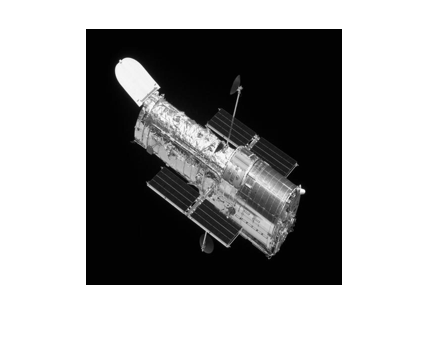
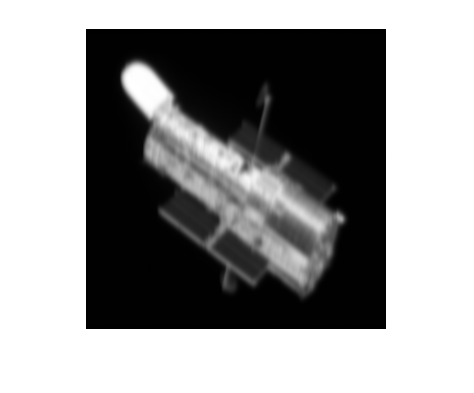
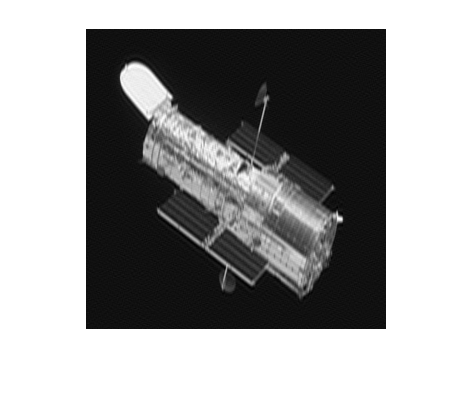
Figure 1: True image (left), blurred and noisy image (middle) with noise level $\widetilde{\delta}=10^{-3}$, and restored image by the tAT (right) method after $8$ iterations.

The restored images determined by the tAT, G-tAT and tGMRES methods are accessed using the $\mathtt{squeeze}$ operator and displayed in Figures 1 and 2 for the noise level $\widetilde{\delta}=10^{-3}$. Similarly, the restored image computed by the GMRES method is displayed in Figure 2 (middle) using MATLAB reshape command.

Table 4 shows the computed regularization parameters,relative errors and PNSR for the noise levels $10^{-2}$ and $10^{-3}$, as well as CPU times. As can be expected, the quality of the computed restorations improves when the noise level is smaller. The tGMRES method requires the least CPU time for $\widetilde{\delta}=10^{-3}$ and yields the worst restorations for both noise levels. Independent of the choice of $\mathcal{L}$, Tikhonov regularization implemented by the tAT method determines restorations of the highest quality. The G-tAT and G-tGMRES methods, which involve flattening, demand the most CPU times and require the most iterations for both noise levels. The GMRES and G-tGMRES methods require the same number of iterations and yield the same quality restorations for both noise levels. Similar observations can be made for the AT and G-tAT methods when the regularization operator is the identity matrix and identity tensor, respectively.

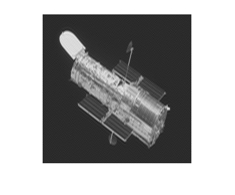
Figure 2: Restored images by the G-tAT (left), GMRES (middle), and tGMRES (right) methods after $51$, $51$, and $8$ iterations, respectively, for the noise level $\widetilde{\delta}=10^{-3}$.

$\mathcal{L}$	Noise level	Method	$\ell$	$\mu_{\ell}$	PSNR	Relative error	CPU time (secs)
$\mathcal{L}_{1}$	$10^{-3}$	tAT	8	2.27e+04	29.09	1.19e-01	35.14
		G-tAT	51	3.18e+04	28.04	1.34e-01	977.90
	$10^{-2}$	tAT	3	4.43e+01	26.81	1.53e-01	7.23
		G-tAT	12	3.98e+02	25.30	1.84e-01	63.50
$\mathcal{I}$	$10^{-3}$	tAT	8	9.26e+04	29.05	1.19e-01	27.39
		G-tAT	51	1.11e+05	28.04	1.34e-01	910.96
	$10^{-2}$	tAT	3	1.34e+03	26.99	1.51e-01	5.41
		G-tAT	12	1.86e+03	25.21	1.86e-01	52.29
	$10^{-3}$	AT	51	1.11e+05	28.04	1.34e-01	60.05
	$10^{-2}$	AT	12	1.90e+03	25.21	1.86e-01	2.76
	$10^{-3}$	GMRES	51	-	27.97	1.35e-01	59.91
		tGMRES	8	-	20.28	2.03e-01	24.43
		G-tGMRES	51	-	27.97	1.35e-01	898.32
	$10^{-2}$	GMRES	12	-	24.94	1.91e-01	2.64
		tGMRES	3	-	17.74	4.39e-01	3.40
		G-tGMRES	12	-	24.94	1.91e-01	50.91

Table 4: Results for Example 6.3.

Example 6.4.

(Color image restoration) This example is concerned with the restoration of color images using the same regularization operators as in Example 6.3. We seek to determine an approximate solution of the image deblurring problem

$$(A_{1}\otimes A_{2})X=B,$$ (6.6)

where the desired unavailable blur- and noise-free image $X_{\rm true}\in\mathbb{R}^{300^{2}\times 3}$ is the matricized three-channeled image $\mathcal{X}_{\rm true}\in\mathbb{R}^{300\times 300\times 3}$. The right-hand side $B\in\mathbb{R}^{300^{2}\times 3}$ in (6.6) is generated by $B=(A_{1}\otimes A_{2})X_{\rm true}+E$, where the unknown noise in the matrix $B$ is represented by $E\in\mathbb{R}^{300^{2}\times 3}$, which is the matricized “noise” tensor $\mathcal{E}\in\mathbb{R}^{300\times 300\times 3}$. The blurring matrices $A_{1}$ and $A_{2}$ are defined by (6.3) in Example 6.3 with $N=300$, $\sigma=3$ and ${\tt band}=12$. By the same reasoning as in Example 6.3, we formulate (6.6) as the 3D image deblurring problem

$$\mathcal{A*X}=\mathcal{B},$$ (6.7)

where the blurring tensor $\mathcal{A}\in\mathbb{R}^{300\times 300\times 300}$ is constructed by (6.5) in Example 6.3. The computed condition numbers of the frontal slices of $\mathcal{A}$ are $\mathtt{cond}(\mathcal{A}^{(i)})=7.6\cdot 10^{8}$ for $i=1,2,\dots,12$, and $\mathtt{cond}(\mathcal{A}^{(i)})$ is “infinite” for $i\geq 13$. We determine the regularization parameter(s) by the bisection method over the interval $[10^{-5},10^{7}]$. The discrepancy principle is used with the parameter $\eta=1.1$. The (standard) global GMRES (G-GMRES) and (standard) global Arnoldi-Tikhonov (GAT) methods for (6.6) are based on the global Arnoldi process applied by Huang et al. [20]. We compare the performance of these methods to the tAT_p, nested$\_$tAT_p, G-tAT_p, GG-tAT, tGMRES_p, G-tGMRES_p, and GG-tGMRES methods for the solution of (6.7).

The original (blur- and noise-free) flower image shown on the left-hand side of Figure 3 is stored as a tensor $\mathcal{X}_{\text{true}}\in\mathbb{R}^{300\times 3\times 300}$. It is blurred using the tensor $\mathcal{A}$. Thus, $\mathcal{{B}}_{\text{true}}=\mathcal{A}*\mathcal{{X}}_{\text{true}}\in\mathbb{R}^{300\times 3\times 300}$ represents the blurred but noise-free image associated with $\mathcal{X}_{\text{true}}$. The “noise” tensor $\mathcal{{E}}\in\mathbb{R}^{300\times 3\times 300}$ is generated as described by (6.1) with noise level $\widetilde{\delta}=10^{-3}$ and added to $\mathcal{B}_{\text{true}}$ to obtain the blurred and noisy image $\mathcal{{B}}$ shown in Figure 3 (middle). The latter image is accessed by using the multi$\_$squeeze operator.

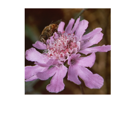
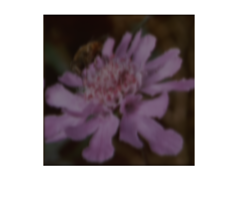
Figure 3: True image (left), blurred and noisy image (middle) with noise level $\widetilde{\delta}=10^{-3}$, and restored image determined by nested$\_$tAT_p (right) after $9$ iterations.

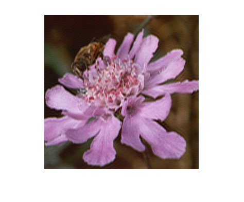
Figure 4: Restored images determined by GG-tAT (left) after $32$ iterations, and G-GMRES (middle) after $32$ iterations and the tGMRES_p (right), for the noise level $\widetilde{\delta}=10^{-3}$.

The restored images determined by the nested$\_$tAT_p, GG-tAT, G-GMRES, and tGMRES methods are displayed in Figures 3 and 4. Relative errors and PSNR as well as CPU times are shown in Table 5. The tAT method gives restorations of the highest quality, followed by the nested$\_$tAT_p method. These methods do not involve flattening. Solution methods that involve flattening such as the G-tAT_p, GG-tAT, G-tGMRES_p, and GG-tGMRES methods require the most CPU time for both noise levels. The GAT, GG-tAT, G-GMRES, and GG-tGMRES methods require the same number of iterations, which are more than the number of iterations used by the nested$\_$tAT_p method for both noise levels. The tGMRES_p method yields restorations of the worst quality for both noise levels. The GG-tGMRES method that works with the whole data tensor at a time yields the same quality restorations as the G-GMRES method for both noise levels. The same conclusion can be drawn for the GG-tAT and GAT methods when the regularization operator is the identity tensor and the identity matrix, respectively. The quality of restorations by the G-tAT_p and GG-tAT methods improves significantly with the use of the regularization operator $\mathcal{L}_{1}$ for both noise levels.

$\mathcal{L}$	Noise level	Method	$\ell$	$\mu_{\ell}$	PSNR	Relative error	CPU time (secs)
$\mathcal{L}_{1}$	$10^{-3}$	tATp	-	-	30.56	5.85e-02	93.08
		nested$\_$tATp	9	-	30.56	5.86e-02	64.79
		G-tATp	-	-	29.47	6.64e-02	1187.47
		GG-tAT	32	7.34e+03	29.43	6.67e-02	894.05
	$10^{-2}$	tATp	-	-	27.20	8.62e-02	21.07
		nested$\_$tATp	4	-	25.90	1.00e-01	21.51
		G-tATp	-	-	25.20	1.09e-01	101.27
		GG-tAT	9	1.51e+02	25.22	1.08e-01	70.43
$\mathcal{I}$	$10^{-3}$	tATp	-	-	30.67	5.78e-02	75.66
		nested$\_$tATp	9	-	30.69	5.77e-02	57.02
		G-tATp	-	-	29.44	6.66e-02	1114.94
		GG-tAT	32	3.64e+04	29.40	6.69e-02	430.23
	$10^{-2}$	tATp	-	-	27.66	8.18e-02	16.64
		nested$\_$tATp	4	-	26.26	9.60e-02	22.88
		G-tATp	-	-	24.96	1.12e-01	82.66
		GG-tAT	9	1.15e+03	24.87	1.13e-01	33.77
	$10^{-3}$	GAT	32	3.63e+04	29.40	6.69e-02	96.86
	$10^{-2}$	GAT	9	1.15e+03	24.87	1.13e-01	6.22
	$10^{-3}$	G-GMRES	32	-	29.33	6.75e-02	98.89
		tGMRESp	-	-	19.23	2.16e-01	69.72
		G-tGMRESp	-	-	29.36	6.73e-02	1105.67
		GG-tGMRES	32	-	29.32	6.75e-02	425.55
	$10^{-2}$	G-GMRES	9	-	24.56	1.17e-01	5.21
		tGMRESp	-	-	12.75	4.55e-01	10.45
		G-tGMRESp	-	-	24.78	1.14e-01	82.35
		GG-tGMRES	9	-	24.56	1.17e-01	33.07

Table 5: Results for Example 6.4.

Example 6.5.

(Video restoration) This example considers the restoration of the first six consecutive frames of the $\mathtt{Xylophone}$ video from MATLAB. Each video frame is in the $\mathtt{MP4}$ format and has $240\times 240$ pixels.

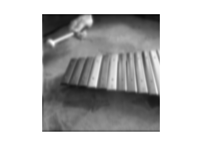
Figure 5: True image (left), blurred and noisy image with noise level $\widetilde{\delta}=10^{-3}$ (middle), and restored image determined by $8$ iterations with the tAT_p method (right).

The first six blur- and noise-free frames are stored as a tensor $\mathcal{X}_{\text{true}}\in\mathbb{R}^{240\times 6\times 240}$ using the $\mathtt{multi}\_\mathtt{twist}$ operator. They are blurred by the tensor $\mathcal{A}\in\mathbb{R}^{240\times 240\times 240}$, which is generated similarly as in Example 6.3 with its frontal slices determined by

$$\mathcal{A}^{(i)}=A_{2}(i,1)A_{2},~{}~{}~{}i=1,2,\dots,n,~{}~{}~{}N=240,~{}~{}\sigma=2.5~{}~{}{\rm and}~{}~{}{\tt band}=12.$$

The condition numbers of the frontal slices of $\mathcal{A}$ are $\mathtt{cond}(\mathcal{A}^{(i)})=1.4\cdot 10^{7}$ for $i=1,2,\dots,12$. The condition numbers of the remaining frontal slices are “infinite”.

We use the regularization operator $\mathcal{L}=\mathcal{L}_{2}\in\mathbb{R}^{239\times 240\times 240}$ and determine the regularization parameter(s) by the bisection method over the interval $[10^{-5},10^{7}]$ using the discrepancy principle with $\eta=1.1$. The blurred and noisy frames are generated by $\mathcal{B}=\mathcal{A}*\mathcal{X}_{\text{true}}+\mathcal{E}\in\mathbb{R}^{240\times 6\times 240}$ with the “noise” tensor $\mathcal{E}\in\mathbb{R}^{240\times 6\times 240}$ defined by (6.1).

The true third frame is displayed in Figure 5 (left), and the blurred and noisy third frame is shown in Figure 5 (middle) using the $\mathtt{squeeze}$ operator. Similarly, the restored images of the third frame determined by the G-tAT_p, nested$\_$tAT_p, G-tGMRES, and tGMRES methods are shown in Figures 5 and 6.

Figure 6: Restored images by the nested$\_$G-tAT_p (left), G-tGMRES_p (middle), and tGMRES_p (right) for $\widetilde{\delta}=10^{-3}$.

The relative errors, PSNR and CPU times are displayed in Table 6. The tAT_p and nested$\_$tAT_p methods, which do not involve flattening, are seen to yield restorations of the highest quality for all noise levels. The tGMRES method is the fastest for $\widetilde{\delta}=10^{-2}$ and $10^{-3}$, but gives the worst restorations for all noise levels. Solution methods that involve flattening, such as tAT_p, GG-tAT and G-tGMRES_p and GG-tGMRES methods, are the slowest for $\widetilde{\delta}=10^{-3}$.

Noise level	Method	$\ell$	$\mu_{\ell}$	PSNR	Relative error	CPU time (secs)
$10^{-3}$	tATp	-	-	34.07	4.15e-02	52.53
	nested$\_$tATp	10	-	33.81	4.27e-02	46.40
	G-tATp	-	-	33.27	4.54e-02	463.08
	GG-tAT	22	7.46e+02	33.24	4.56e-02	203.42
	tGMRESp	-	-	27.21	9.13e-02	31.88
	G-tGMRESp	-	-	33.17	4.60e-02	406.93
	GG-tGMRES	22	-	33.21	4.58e-02	97.66
$10^{-2}$	tATp	-	-	30.75	6.07e-02	20.28
	nested$\_$tATp	3	-	25.64	1.09e-01	18.01
	G-tATp	-	-	27.22	9.12e-02	69.21
	GG-tAT	8	2.16e+02	27.22	9.12e-02	25.74
	tGMRESp	-	-	15.67	3.45e-01	8.23
	G-tGMRESp	-	-	26.82	9.55e-02	52.78
	GG-tGMRES	8	-	26.82	9.55e-02	11.93
$10^{-1}$	tATp	-	-	24.69	1.22e-01	13.84
	nested$\_$tATp	2	-	21.25	1.81e-01	16.94
	G-tATp	-	-	21.17	1.83e-01	5.24
	GG-tAT	2	1.04e+01	21.17	1.83e-01	1.60
	tGMRESp	-	-	0.45	1.99e+00	3.46
	G-tGMRESp	-	-	19.21	2.29e-01	3.16
	GG-tGMRES	2	-	19.21	2.29e-01	0.68

Table 6: Results for Example 6.5.

7 Conclusion

This paper extends the standard Arnoldi iteration for matrices to third order tensors and describes several algorithms based on this extension for solving linear discrete ill-posed problems with a t-product structure. The solution methods are based on computing a few steps of the extended Arnoldi process, which is referred to as the t-Arnoldi process. The global t-Arnoldi and generalized global t-Arnoldi processes also are considered. Differently from the t-Arnoldi process, the latter processes involve flattening. Both Tikhonov regularization and regularization by truncated iteration are illustrated. The latter gives rise to an extension of the standard GMRES method, referred to as the tGMRES and global tGMRES methods. The discrepancy principle is used to determine the number of iterations with the t-Arnoldi, global t-Arnoldi, and generalized global t-Arnoldi processes, as well as the regularization parameter in Tikhonov regularization and the number of iterations by the Arnoldi-type and GMRES-type methods. The effectiveness of the proposed methods is illustrated by applications to image and video restorations. Solution methods such as tAT, tAT_p, and nested$\_$tAT_p that avoid matricization or vectorization of discrete ill-posed problems for tensors show great promise in terms of speed and quality of the computed restorations determined by their relative errors and PSNR when compared to solution methods that matricize or vectorize.

References

• [1] F. P. A. Beik, K. Jbilou, M. Najafi-Kalyani, and L. Reichel, Golub-Kahan bidiagonalization for ill-conditioned tensor equations with applications, Numer. Algorithms, 84 (2020), pp. 1535–1563.
• [2] F. P. A. Beik, M. Najafi-Kalyani, and L. Reichel, Iterative Tikhonov regularization of tensor equations based on the Arnoldi process and some of its generalizations, Appl. Numer. Math., 151 (2020), pp. 425–447.
• [3] A. Buccini, M. Pasha, and L. Reichel, Generalized singular value decomposition with iterated Tikhonov regularization, J. Comput. Appl. Math., 373 (2020), Art. 112276.
• [4] D. Calvetti, B. Lewis, and L. Reichel, On the regularizing properties of the GMRES method, Numer. Math., 91 (2002), pp. 605–625.
• [5] D. Calvetti, S. Morigi, L. Reichel, and F. Sgallari, Tikhonov regularization and the L-curve for large, discrete ill-posed problems, J. Comput. Appl. Math., 123 (2000), pp. 423–446.
• [6] D. Calvetti and L. Reichel, Tikhonov regularization of large linear problems, BIT Numer. Math., 43 (2003), pp. 263–283.
• [7] M. Donatelli, D. Martin, and L. Reichel, Arnoldi methods for image deblurring with anti-reflective boundary conditions, Appl. Math. Comput., 253 (2015), pp. 135–150.
• [8] M. El Guide, A. El Ichi, K. Jbilou, and F. P. A Beik, Tensor GMRES and Golub-Kahan bidiagonalization methods via the Einstein product with applications to image and video processing, https://arxiv.org/pdf/2005.07458.pdf
• [9] A. El Ichi, M. El Guide and K. Jbilou, Discrete cosine transform LSQR and GMRES methods for multidimensional ill-posed problems, March 2021. https://arxiv.org/pdf/2103.11847.pdf
• [10] M. El Guide, A. El Ichi, K. Jbilou, and R. Sadaka, Tensor Krylov subspace methods via the T-product for color image processing, June 2020. https://arxiv.org/pdf/2006.07133.pdf
• [11] G. Ely, S. Aeron, N. Hao, and M. E. Kilmer, 5d and 4d pre-stack seismic data completion using tensor nuclear norm (TNN), SEG International Exposition and Eighty-Third Annual Meeting at Houston, TX, 2013.
• [12] H. W. Engl, M. Hanke, and A. Neubauer, Regularization of Inverse Problems, Kluwer, Dordrecht, 1996.
• [13] C. Fenu, L. Reichel, and G. Rodriguez, GCV for Tikhonov regularization via global Golub-Kahan decomposition, Numer. Linear Algebra Appl., 23 (2016), pp. 467–484.
• [14] S. Gazzola, P. Novati, and M. R. Russo, On Krylov projection methods and Tikhonov regularization, Electron. Trans. Numer. Anal., 44 (2015), pp. 83–123.
• [15] G. H. Golub, M. Heath, and G. Wahba, Generalized cross-validation as a method for choosing a good ridge parameter, Technometrics, 21 (1979), pp. 215–223.
• [16] P. C. Hansen, Analysis of discrete ill-posed problems by means of the L-curve, SIAM Rev., 34 (1992), pp. 561–580.
• [17] P. C. Hansen, Rank-Deficient and Discrete Ill-Posed Problems, SIAM, Philadelphia, 1998.
• [18] P. C. Hansen, Regularization tools version 4.0 for MATLAB 7.3. Numer. Algorithms, 46 (2007), pp. 189–194.
• [19] N. Hao, M. E. Kilmer, K. Braman, and R. C. Hoover, Facial recognition using tensor-tensor decompositions, SIAM J. Imaging Sci., 6 (2013), pp. 437–463.
• [20] G. Huang, L. Reichel, and F. Yin, On the choice of subspace for large-scale Tikhonov regularization problems in general form, Numer. Algorithms, 81 (2019), pp. 33–55.
• [21] E. Kernfeld, M. Kilmer, and S. Aeron, Tensor-tensor products with invertible linear transforms, Linear Algebra Appl., 485 (2015), pp. 545–570.
• [22] M. Kilmer, K. Braman, and N. Hao, Third order tensors as operators on matrices: A theoretical and computational framework, Tufts University, Department of Computer Science, Tech. Rep., January 2011.
• [23] M. E. Kilmer, K. Braman, N. Hao, and R. C. Hoover, Third-order tensors as operators on matrices: A theoretical and computational framework with applications in imaging, SIAM J. Matrix Anal. Appl., 34 (2013), pp. 148–172.
• [24] M. E. Kilmer and C. D. Martin, Factorization strategies for third-order tensors, Linear Algebra Appl., 435 (2011), pp. 641–658.
• [25] S. Kindermann, Convergence analysis of minimization-based noise level-free parameter choice rules forlinear ill-posed problems, Electron. Trans. Numer. Anal., 38 (2011), pp. 233–257.
• [26] S. Kindermann and K. Raik, A simplified L-curve method as error estimator. Electron. Trans. Numer. Anal., 53 (2020), pp. 217–238.
• [27] T. G. Kolda and B. W. Bader, Tensor decompositions and applications, SIAM Rev., 51 (2009), pp. 455–500.
• [28] B. Lewis and L. Reichel, Arnoldi-Tikhonov regularization methods, J. Comput. Appl. Math., 226 (2009), pp. 92–102.
• [29] C. Lu, J. Feng, Y. Chen, W. Liu, Z. Lin, and S. Yan, Tensor robust principal component analysis with a new tensor nuclear norm, IEEE Trans. Pattern Anal. Mach. Intell., 42 (2020), pp. 925–938, doi:10.1109/TPAMI.2019.2891760.
• [30] K. Lund. The tensor t-function: a definition for functions of third-order tensors. ArXiv preprint, arXiv:1806.07261, 2018.
• [31] C. D. Martin, R. Shafer, and B. LaRue, An order-$p$ tensor factorization with applications in imaging. SIAM J. Sci. Comput., 35 (2013), pp. A474–A490.
• [32] A. Neubauer, Augmented GMRES-type versus CGNE methods for the solution of linear ill-posed problems, Electron. Trans. Numer. Anal., 51 (2019), pp. 412–431.
• [33] Y. Miao, L. Qi and Y. Wei, T-Jordan Canonical Form and T-Drazin Inverse Based on the T-Product. Commun. Appl. Math. Comput. (2020). https://doi.org/10.1007/s42967-019-00055-4
• [34] Y. Miao, L. Qi and Y. Wei, Generalized tensor function via the tensor singular value decomposition based on the T-product. Linear Algebra and its Applications, 590 (2020) 258-303.
• [35] L. Reichel and A. Shyshkov, A new zero-finder for Tikhonov regularization, BIT Numer. Math., 48 (2008), pp. 627–643.
• [36] L. Reichel and U. O. Ugwu, The tensor Golub-Kahan-Tikhonov method applied to the solution of ill-posed problem with a t-product structure, 2020, submitted for publication.
• [37] L. Reichel and G. Rodriguez, Old and new parameter choice rules for discrete ill-posed problems, Numer. Algorithms, 63 (2013), pp. 65–87.
• [38] Y. Saad, Iterative Methods for Sparse Linear Systems, 2nd ed., SIAM, Philadelphia, 2003.
• [39] Y. Saad and M. H. Schultz, GMRES: a generalized minimal residual method for solving nonsymmetric linear systems, SIAM J. Sci. Stat. Comput., 7 (1986), pp. 856–869.
• [40] B. Savas and L. Eldén, Krylov-type methods for tensor computations, Linear Algebra Appl., 438 (2013), pp. 891–918.
• [41] S. Soltani, M. E. Kilmer, and P. C. Hansen, A tensor-based dictionary learning approach to tomographic image reconstruction, BIT Numer. Math., 56 (2015), pp. 1425–1454.
• [42] L. N. Trefethen and D. Bau III, Numerical Linear Algebra, SIAM, Philadelphia, 1997.
• [43] Z. Zhang, G. Ely, S. Aeron, N. Hao, and M. E. Kilmer, Novel methods for multilinear data completion and de-noising based on tensor-svd, In 2014 IEEE Conference on Computer Vision and Pattern Recognition, CVPR 2014, Columbus, OH, USA, June 23-28, 2014, pp. 3842–3849.