Sideward contact tracing and the control of epidemics in large gatherings

Abstract

Effective contact tracing is crucial to contain epidemic spreading without disrupting societal activities especially in the present time of coexistence with a pandemic outbreak. Large gatherings play a key role, potentially favouring superspreading events. However, the effects of tracing in large groups have not been fully assessed so far. We show that beside forward tracing, which reconstructs to whom disease spreads, and backward tracing, which searches from whom disease spreads, a third “sideward” tracing is always present, when tracing gatherings. This is an indirect tracing that detects infected asymptomatic individuals, even if they have neither been directly infected by, nor they have directly transmitted the infection to the index case. We analyse this effect in a model of epidemic spreading for SARS-CoV-2, within the framework of simplicial activity-driven temporal networks. We determine the contribution of the three tracing mechanisms to the suppression of epidemic spreading, showing that sideward tracing induces a non-monotonic behaviour in the tracing efficiency, as a function of the size of the gatherings. Based on our results, we suggest an optimal choice for the sizes of the gatherings to be traced and we test the strategy on an empirical dataset of gatherings in a University Campus.

I Introduction

Public debate about measures to curb pandemic spreading in the present time, where new extensive outbreaks of SARS-CoV-2 are emerging due to highly transmissible variants, is dominated by opposite tensions toward contrasting goals. On the one hand many advocate the continued implementation of strict policies aimed at preventing virus propagation and all the resulting consequences in terms of deaths, sufferings and long-lasting health problems [1, 2, 3]. On the other hand the heavy economic, societal and psychological costs of restrictions push many to call for lifted restrictions and a general rapid return to normal activities [4, 5, 6]. Finding an acceptable tradeoff between these two clashing tendencies is extremely hard. Decisions must necessarily be taken by policy-makers, but it is the task of science to provide informed advice and predict likely scenarios [7, 2, 8, 9].

A key role in epidemic spreading is played by large gatherings of people, which are fundamental structures of social networks [10, 11, 12]. Indeed one of the most common measures taken by governments to limit disease propagation is the prohibition to hold gatherings above a given size, to suppress the chance of ’superspreading events’ (SSEs), where a large number of people are simultaneously infected [13, 14, 15, 16]. A firm theoretical underpinning for these types of decisions is still lacking. Recent results have shown that large gatherings may have dramatic effects when ’complex contagion’ is at work, i.e. the probability of transmission depends nonlinearly on the number of independent exposures an individual is subjected to [17]. This is however not the typical case for disease spreading (simple contagion), where contact with two infectious individuals simply doubles the contagion probability. Nevertheless the meeting of large groups implies the formation of a quadratically large number of contacts and for this reason limitations to the size of allowed gatherings has a substantial impact on epidemic propagation [18]. In this paper, we show that the specific nature that makes large gatherings threatening, on the other hand can improve the effectiveness of contact tracing procedures and therefore control the spreading process without disrupting societal activities.

The tracing of contacts of infected individuals and their subsequent isolation is one of the main weapons against disease spreading, in particular when pre-symptomatic and asymptomatic individuals are responsible for a large share of transmission events [19, 20]. In the absence of contact tracing, all presymptomatic and asymptomatic infections can go undetected as observed with SARS-CoV-2 [21, 9, 8, 22]. In the usual framework where only binary contacts occur, two types of contact tracing (CT) are possible when somebody is found infected: backward CT follows the transmission chain back in time, aiming at reconstructing who infected the index case [23, 24, 25]; forward CT instead looks for people potentially infected upon contact with the index case prior to his/her detection [23, 24, 25]. In the case of a gathering, if the group is traced as a whole, the efficacy of the procedure is greatly enhanced because of an indirect effect that we dub sideward CT, qualitatively different from the two other tracing types. Sideward CT allows to indirectly trace infected asymptomatic individuals that have participated in the same gathering, even if they have neither been directly infected by the index case nor they have directly infected him/her. We analyze this effect by considering a model of epidemic spreading (tailored to describe SARS-CoV-2 transmission) on a temporal network with groups activation [26], a standard modelling scheme for mutually interacting groups of people evolving with time. In this framework we determine analytically the contribution of each of the three types of tracing to the suppression of epidemic spreading, revealing the great importance of sideward tracing. We show that due to the simultaneous contribution of the three mechanisms, the effectiveness of tracing gatherings is non-monotonic as a function of the gathering size. In particular, the effectiveness features a maximum, where the contact tracing including all the three mechanism is maximally effective. We test our results on synthetic group size distributions and on an empirical dataset for gatherings in a University Campus, whose group distribution is determined via WIFI data, and we suggest an optimal strategy to choose the typical size of the gatherings to be traced. This optimal tracing of large gatherings can readily offset their potential for disease spreading, thus providing a concrete strategy to curb epidemics still allowing activities to proceed with limited restrictions.

II Results

II.1 Epidemic spreading on simplicial temporal networks

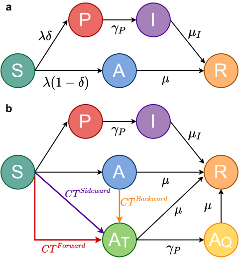
Figure 1: The epidemic compartmental model with and without tracing. a Scheme of the transitions in the compartmental epidemic model without CT. b The enlarged compartmental model in the presence of forward, backward and sideward CT. The transition rates for infections and for CT are discussed in details in the text and in the Supplementary Material, SM.

Temporal networks constitute a general framework developed in recent years, to model systems in which interactions among elements are continuously added and removed, typically on the same temporal scale of the process that is considered on the network [27]. In particular, in activity-driven networks the activation of the links is determined by the activity of the nodes [28, 29, 30]. Here we focus on activity-driven simplicial temporal networks, in which the temporal dynamics of social contacts occurs in groups, accounting for the higher-order nature of interactions [26, 11, 12].

In particular, we consider individuals as nodes of a temporal network, that interact with others by taking part in gatherings, modelled as simplices: each node in a gathering is in contact with all the others forming thus a fully connected cluster. The interaction network evolves by activating simplices at rate $a$, the simplex activity; when a $(s-1)$-simplex (i.e. a clique of size $s$) is active, $s$ nodes are chosen uniformly at random to participate in the simplex, producing $s(s-1)/2$ interactions. Then the links are destroyed and the process is iterated. The simplex size $s$ is drawn from a distribution $\Psi(s)$ that models the heterogeneity in the size of gatherings. Usual pairwise interactions correspond to simplices with $s=2$. On top of this network, the pathogen spreading dynamics is described by a compartmental model (see Fig. 1a) accounting for the main stages of a contagious disease with asymptomatic and pre-symptomatic transmission, such as SARS-CoV-2 infection [22, 31, 32]. A susceptible individual $S$ is infected with probability $\lambda$ if connected with an infected node by a link of the temporal simplex. Infected individuals branch out in two paths: the infection can be symptomatic with probability $\delta$, $S\xrightarrow[]{\lambda\delta}P$, or asymptomatic with probability $(1-\delta)$, $S\xrightarrow[]{\lambda(1-\delta)}A$. Asymptomatic nodes $A$ spontaneously recover ($R$) with rate $\mu=1/\tau$; pre-symptomatic individuals spontaneously develop symptoms with rate $\gamma_{P}=1/\tau_{P}$, thus with a Poissonian process $P\xrightarrow[]{\gamma_{P}}I$, and then infected symptomatic $I$ spontaneously recover with rate $\mu_{I}=\mu\gamma_{P}/(\gamma_{P}-\mu)$. The average infectious period is therefore $\tau$ both for asymptomatic and symptomatic individuals. Susceptible $S$, recovered $R$, asymptomatic $A$ and pre-symptomatic $P$ individuals have an equal uniform probability to join a simplex. Over this temporal network we introduce an adaptive behavior, assuming that symptomatic individuals $I$ are immediately isolated and thus are not able to participate in simplices and propagate the infection [33, 34, 35, 36].

SIR compartmental models are characterised by an active phase, in which the epidemic propagates to a finite fraction of nodes, and an absorbing phase with the number of infected individuals exponentially decaying to zero. The epidemic threshold separating the two phases can be analytically obtained by means of a linearisation procedure, providing the stability of the absorbing phase. In particular in activity-driven models the calculation of the threshold is exact since local correlations are continuously destroyed by link reshuffling [28, 29, 30]. We use the infection probability $\lambda$ as control parameter; i.e. only above its critical value $\lambda_{C}$ – the epidemic threshold – extensive outbreaks reach a finite fraction of the population. The effectiveness of a control strategy can be estimated by the increase of $\lambda_{C}$. In the simplicial temporal network with no adaptive measures (NA) the threshold is [26]:

$$\lambda_{C}^{NA}=\frac{\mu}{a\langle s(s-1)\rangle},$$ (1)

where $\langle f(s)\rangle$ denotes the average over the different simplex sizes $\langle f(s)\rangle=\int ds\,\Psi(s)f(s)$. Notice that the critical condition can be reformulated in terms of the basic reproduction number $R_{0}$, which is defined as $R_{0}=\lambda/\lambda_{C}^{NA}=\lambda a\langle s(s-1)\rangle/\mu$.

If symptomatic individuals $I$ are immediately and perfectly isolated once they develop symptoms, the epidemic threshold is (see the Supplementary Material - SM, Section I.D for details):

$$\lambda_{C}^{sympto}=\lambda_{C}^{NA}\frac{\frac{\gamma_{P}}{\mu}}{\delta+\frac{\gamma_{P}}{\mu}(1-\delta)}.$$ (2)

Also in this case the concept of epidemic threshold can be reframed in terms of the reproduction number $R_{0}$, which is defined as $R_{0}=\lambda/\lambda_{C}^{sympto}=\frac{\lambda a\langle s(s-1)\rangle}{\mu}\frac{\delta+(1-\delta)\gamma_{P}/\mu}{\gamma_{P}/\mu}$. In Eq. (2) for $\delta=0$ (no symptomatic infection) we recover Eq. (1), while for $\delta=1$ the epidemic transmission is maximally reduced due to isolation of symptomatic individuals. This increases $\lambda_{C}$ of a factor $\frac{\gamma_{P}}{\mu}$. Hereafter, $\lambda_{C}^{sympto}$ will be the reference for the evaluation of the performance of CT strategies.

II.2 Contact tracing mechanisms in simplices

We consider a traditional (non app-based) CT process [36] on simplices: the goal is to identify and isolate infected asymptomatic individuals. Note that since individuals in state $I$ are instantaneously isolated, they do not participate in simplices. Only individuals in state $P$ or $A$ may spread the infection. Within this assumption presymptomatic individuals also represent people with no symptoms or very weak ones, thus still able to attend events, at least for a certain time before isolation (imperfect isolation). CT is activated when a presymptomatic individual develops significant symptoms $P\to I$: in such a case each simplex he/she has participated in during the previous $T_{CT}$ days is traced as a whole, with a probability $\epsilon(s)$. Each node belonging to a traced simplex is tested and, if found in the asymptomatic infected (A) state, isolated. The tracing procedure is stopped at the first-step, so we do not consider iterative tracing. The probability of tracing a simplex can depend in general on the size $s$: people typically remember only some of the gatherings they joined; some simplices are easily fully traced (e.g. school classes, workplace meetings) while others are not easily reconstructed (e.g. interactions on public transportation, shops, restaurants). The dependence of $\epsilon(s)$ on the simplex size $s$ also allows to model tracing strategies targeted at groups of a given size.

In the present framework CT is modelled by introducing two additional compartments for asymptomatic individuals (see Fig. 1b): traced asymptomatic, $A_{T}$, and quarantined asymptomatic, $A_{Q}$. An $A_{T}$ node is asymptomatic and infective, just as an $A$ individual, but it has been in touch with a pre-symptomatic individual who remembers the gathering where the contact took place. We assume that tracing time is shorter than the typical time of the epidemic evolution, so that it can be considered instantaneous. Therefore, when the pre-symptomatic develops symptoms, the $A_{T}$ node enters quarantine and becomes an $A_{Q}$ node, which is isolated and hence does not participate in simplices. We describe the effect of isolation of contacts occurring when the index node develops symptoms setting the transition $A_{T}\to A_{Q}$ at the same rate $\gamma_{P}$ for the appearance of symptoms (see [36] for a discussion on the effects of longer tracing times).

Besides these assumptions, our model involves other hypotheses in the tracing procedure and in the epidemic transmission. For example, we assume that all nodes within a traced simplex are identified and that, once the nodes are found infected, the isolation of quarantined individuals is perfect. We also assume that symptomatic and asymptomatic individuals have the same infectivity and that the probability of infection is independent of the simplex size. All these assumptions can be relaxed in the model in a straightforward manner, by including new parameters or interdependences between the parameters with no conceptual obstacles. We do not expect this to modify substantially our findings on the general behaviour of the tracing procedure that we are going to discuss.

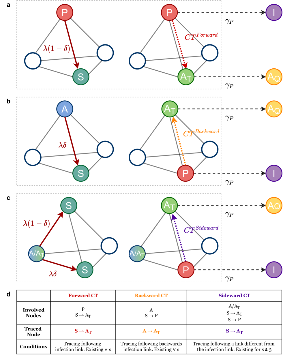
Figure 2: Contact tracing mechanisms in simplices: forward, backward and sideward CT. a Scheme of the forward CT. b Scheme of the backward CT. c Scheme of the sideward CT: note that in this case the CT can be activated both if the infected node is $A$ or $A_{T}$. Moreover in this simplex also backward CT can occur on the node $A$, if present, activated by $S\to P$, but for simplicity we do not show it in the scheme. Finally, sideward CT can be activated if the asymptomatic and symptomatic infections are produced by two different asymptomatic individuals (or traced asymptomatics), who participate in the simplex; this process is considered in the model (see SM) and produce a term quadratic in the density of asymptomatic nodes. However for simplicity in the scheme we consider the first-order term, which is the only one to survive the linearisation for the calculation of the epidemic threshold. In all the tracing mechanisms, the traced node becomes $A_{T}$ upon contact with the index case and then is isolated $A_{T}\to A_{Q}$ at the same rate $\gamma_{P}$ for the appearance of symptoms in the index case $P\to I$, assuming the tracing time shorter then the typical time of the epidemic evolution, so that it can be considered instantaneous. d Summary of the main features of the three CT mechanisms.

Inside simplices three types of contact tracing mechanisms are at work: forward and backward CT, already present for pairwise interactions [36, 25, 23, 24], are augmented by sideward CT, which is specific of simplices traced as a whole.

Forward CT looks for asymptomatic individuals infected by a presymptomatic index case who, upon developing symptoms, activates the CT. This mechanism involves, in the simplex, one susceptible node and a presymptomatic index case (see Fig. 2a). At the moment of the infection event, the susceptible node becomes asymptomatic and traced ($A_{T}$), the tracing occurs along the same link on which the infection takes place. See Methods for the associated term in the mean-field equations.

Backward CT is the search for the source of infection of a symptomatic index case, who activates the CT. This mechanism is at work when in a simplex an asymptomatic node infects a susceptible node making it presymptomatic (see Fig. 2b): the asymptomatic node is traced (becoming $A_{T}$) along the contact that produced the infection, but the tracing goes in the opposite direction. The asymptomatic node traced in the process is already infected when he/she enters the simplex, thus the tracing occurs after the infection event and after he/she has potentially infected other nodes. See Methods for the associated term in the mean-field equations.

Sideward CT finds asymptomatic nodes infected by other asymptomatic individuals, by exploiting the presence in the simplex of a third node that develops symptoms (see Fig. 2 c). Therefore, sideward CT occurs when in the simplex there is at least one asymptomatic $A$ (or traced asymptomatic $A_{T}$) node, that infects a susceptible node (that becomes asymptomatic) and also infects at least another susceptible node (that becomes presymptomatic). The participation in the same simplex implies that the asymptomatic is traced so that it enters quarantine when the presymptomatic develops symptoms and activates CT. Another possibility is that the two susceptible nodes in Fig. 2 c are infected by different asymptomatic individuals, however the term associated to this process is quadratic in the density of asymptomatic nodes and hence does not influence the threshold value. Sideward CT requires the presence of at least three nodes, thus it is active only if $s\geq 3$; moreover it occurs ”laterally”, since the traced contact does not transmit the infection. Note that in the same simplex also backward CT can be activated on the infector if it is an infected asymptomatic $A$. In the linearised mean-field equations (see Methods), sideward CT is described by a transition from $S$ directly to $A_{T}$ with the following term:

$$C^{Sideward}=a\lambda(1-\delta)\left\langle\epsilon(s)s(s-1)\left[1-(1-\lambda\delta)^{(s-2)}\right]\right\rangle[A(t)+A_{T}(t)],$$ (3)

where $a$ is the simplex activation rate, the probability to take part to the simplex for the susceptible node is proportional to $s$ and, in the linearised regime, the probability that among the remaining $(s-1)$ nodes there is an asymptomatic (or a traced symptomatic) node is $(s-1)[A(t)+A_{T}(t)]$. The asymptomatic infection occurs with probability $\lambda(1-\delta)$ and $\left[1-(1-\lambda\delta)^{(s-2)}\right]$ is the probability that, at least in one of the remaining $(s-2)$ nodes, a symptomatic contagion occurs. $\epsilon(s)$ is the probability that the simplex is traced and the term is averaged over all simplex sizes.

The CT terms feature a highly non-trivial dependence on the control parameter $\lambda$ (see Eq. (3), Methods and SM): this complicates the calculation of the epidemic threshold $\lambda_{C}$ (see SM) and prohibits to formulate the reproduction number $R_{0}$ as a simple function of $\lambda$, unlike the case with only symptomatic isolation. Thus, hereafter we will describe the critical behaviour by means of the epidemic threshold $\lambda_{C}$. Again, the goal of CT is to increase the threshold: the more effective the CT strategy, the higher the value of $\lambda_{C}$.

II.3 The effects of forward, backward and sideward tracing in simplices

The three tracing mechanisms contribute differently to the epidemic mitigation and their effectiveness depends on the structure of interactions, i.e. the simplex distribution $\Psi(s)$. To compare their performance we assume that the probability to be traced is equal for simplices of any size, i.e. $\epsilon(s)=\epsilon,\,\forall s$. We keep constant $\overline{n}=a\langle s(s-1)\rangle$, the average number of contacts per individual per time unit, so that different distributions $\Psi(s)$ correspond to the same number of interactions, arranged in simplices of different size. We assess the specific effect of each CT by calculating the threshold first when only symptomatic individuals are isolated, then with each CT mechanism at work separately and finally when all CTs are active (see Methods and SM). In Fig. 3 a-b we consider all simplices of the same size $\overline{s}$, i.e. $\Psi(s)=\delta(s-\overline{s})$, where $\delta(x)$ is the Dirac delta-function, while in Fig. 3 c-d an exponential distribution $\Psi(s)\sim e^{-\beta s}$ is considered, with $s\in[2,\infty)$. Finally, in Fig. 3 e-f the simplex size distribution is a power-law $\Psi(s)\sim s^{-(\nu+1)}$, with $s\in[2,s_{M}]$ and $s_{M}$ being of the order of hundreds of nodes, as often observed in real systems [10]. The effects of the isolation of symptomatics and of forward CT are independent of $\Psi(s)$, while backward and sideward CT strongly depend on $\Psi(s)$. Sideward tracing is very effective in the presence of large simplices, where lateral tracing is more probable, while it cannot be triggered for $s=2$ (i.e. simple links). In large simplices, sideward CT is indeed able to trace all new asymptomatic individuals and isolate them at the infection, avoiding epidemic spreading and the explosive effects of SSEs. On the other hand, backward tracing is more effective on small simplices: in large clusters, with many contacts, it only traces the source of infection, while other simultaneous contagions may occur and go undetected.

Interestingly, when all CT mechanisms are at work, the combination of backward and sideward tracing gives rise to a non-monotonic behaviour as a function of the simplex size. In particular, the threshold features a maximum, where CT is maximally effective. In networks with a single simplex size or with a sharp exponential distribution, the size corresponding to this maximum is of the order of $100$ nodes, while for broader distributions, with very large clusters dominating the transmission even at small $\langle s\rangle$, the tracing is maximally effective when $\langle s\rangle\approx 10$. The position of this maximum strongly depends also on the fraction of asymptomatic nodes (see SM). In particular, a large fraction of asymptomatic nodes is most effectively traced by sideward tracing while for few asymptomatics backward tracing is most effective.

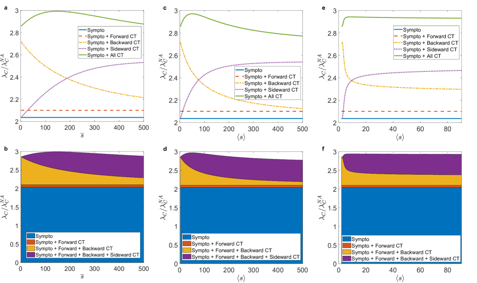
Figure 3: The effects of forward, backward and sideward contact tracing. a We consider $\Psi(s)=\delta(s-\overline{s})$ and we plot, as a function of $\overline{s}$, the ratio between the epidemic threshold $\lambda_{C}$ when symptomatic isolation and CT are activated and the epidemic threshold $\lambda_{C}^{NA}$ of the non-adaptive case. We plot curves corresponding to the activation of each CT mechanism alone and then to the case when they are all active. b For the same $\Psi(s)$ of panel a we plot the ratio $\lambda_{C}/\lambda_{C}^{NA}$ as a function of $\overline{s}$ for symptomatic isolation and activating progressively all CT mechanisms. c and d: As in panels a and b, respectively, but for $\Psi(s)\sim e^{-\beta s}$, with $s\in[2,\infty)$. e and f: As in panels a and b, respectively, but for $\Psi(s)\sim s^{-(\nu+1)}$ and $s\in[2,500]$. In panels c-d and e-f we change the average simplex size $\langle s\rangle$, by varying $\beta$ and $\nu$, respectively, thus changing the tails of the $\Psi(s)$ distribution. In all panels $\epsilon(s)=0.3\,\forall s$. All the other parameters are fixed as discussed in the Methods.

II.4 Optimal strategies for contact tracing in a real setting

In the presence of large simplices, epidemic diffusion is mainly driven by SSEs, with many infections in few large gatherings. This suggests to focus tracing efforts specifically on large simplices. We quantitatively test this hypothesis by comparing the impact of the different tracing mechanisms in a realistic situation. We use $\Psi(s)$ distributions measured empirically at the University of Parma (Italy) by considering simultaneous connections to Access Points (APs) of the university WIFI network as proxies of gatherings (see Methods, Fig. 4a and Fig. 5). Only epidemiologically significant gatherings, i.e. lasting longer than 15 minutes [37], are considered: note that indoor airborne transmission of SARS-CoV-2 has been observed to occur on spatial scales comparable to those covered by WIFI APs [38], making WIFI a good tool to support traditional CT [39]. Two separate distributions $\Psi(s)$ (see Fig. 4a) are calculated for time periods with two different levels of activity restrictions: partial opening and closure of the University [40] (see Methods).

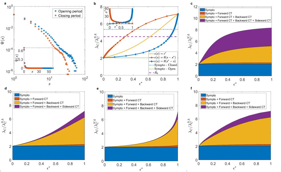
Figure 4: Tracing strategies on empirical University gatherings data. a We plot the distributions $\Psi(s)$ obtained via WIFI data for the University of Parma during the partial opening and closure periods. The main plot is in log-log scale, while in the inset the same distributions are plotted in linear scale. b We plot the ratio $\lambda_{C}/\lambda_{C}^{NA}$ as a function of $\epsilon^{*}=\frac{\langle\epsilon(s)(s-1)\rangle}{\langle s-1\rangle}$, where $\lambda_{C}^{NA}$ is the epidemic threshold in the non-adaptive case and $\lambda_{C}$ is the threshold when isolation of symptomatic individuals and CT are activated. We consider the empirical $\Psi(s)$ during the partial opening period and the three CT strategies. The three horizontal lines are: the ratio $\lambda_{C}^{opening}/\lambda_{C}^{NA}\approx 2.04$ when only symptomatic individuals are isolated during the partial opening period (dotted); the value of $R_{0}=\lambda/\lambda_{C}^{NA}=4.5$ for a variant of SARS-CoV-2 (dashed); the ratio $\lambda_{C}^{closure}/\lambda_{C}^{NA}\approx 2.63\lambda_{C}^{opening}/\lambda_{C}^{NA}\approx 5.35$ when only symptomatic individuals are isolated during the closure period (dot-dashed). In the inset it is plotted $s^{*}$ as a function of $\epsilon^{*}$ for the two targeted tracing strategies. c We plot the ratio $\lambda_{C}/\lambda_{C}^{NA}$ as a function of $\epsilon^{*}$ for symptomatic isolation and activating progressively all CT mechanisms, considering $\Psi(s)\sim s^{-(\nu+1)}$, with $s\in[2,200]$ and $\nu=1.5$ and implementing a tracing strategy targeted at large simplices. d Same of panel c with the empirical distribution $\Psi(s)$ during the partial opening and implementing a uniform tracing strategy. e Same of panel d implementing a tracing strategy targeted at small simplices. f Same of panel d implementing a tracing strategy targeted at large simplices. In all panels the parameters are fixed as discussed in Methods.

Both are heterogeneous, as observed in other datasets [10]. The distribution in the closure period features a reduced upper cut-off, due to the restrictions on activities involving many people, such as in-person classes. Consistently, the probability of simplices of size $s=0,1$ (i.e. 0 or 1 individual connected to the AP) is significantly increased.

The variation in $\Psi(s)$ has a strong impact on the epidemic threshold. Assuming that only isolation of symptomatic individuals is active in the partial opening period, the epidemic threshold increases, due to the closure, by a factor

$$\frac{\lambda_{C}^{closure}}{\lambda_{C}^{opening}}=\frac{\langle s(s-1)\rangle_{opening}}{\langle s(s-1)\rangle_{closure}}\simeq 2.63,$$ (4)

so that $\lambda_{C}^{closure}/\lambda_{C}^{NA}\simeq 5.35$. This change comes at the cost of stopping all teaching and most working activities. CT aims at keeping activities unchanged while still controlling the epidemic; we estimate the effect of the CT strategies during the partial opening period and compare the mitigation due to tracing with that due to closure.

Tracing strategies are modelled through different $\epsilon(s)$. The case $\epsilon(s)=\theta(s-s^{*})$, with $\theta(x)$ the Heaviside step function, represents a tracing targeted at large simplices, with size $s\geq s^{*}$, while smaller gatherings are not traced. This strategy is compared with the uniform tracing adopted in the previous section and with tracing applied only to small simplices, $\epsilon(s)=\theta(s^{*}-s)$. In the comparison, we keep constant the resources allocated for tracing, i.e. the average fraction of traced nodes $\epsilon^{*}=\frac{\langle\epsilon(s)(s-1)\rangle}{\langle s-1\rangle}$ (in the uniform case $\epsilon(s)=\epsilon^{*}$ $\forall s$, while in targeted strategies $\epsilon^{*}$ determines the size $s^{*}$). As shown in Fig. 4b, tracing targeted at large simplices is most effective, since it is sufficient to trace on average a small fraction of nodes $\epsilon^{*}$ to obtain a significant increase of the threshold. On the contrary, tracing only small simplices requires almost all gatherings to be traced to obtain a comparable result. Tracing targeted at large simplices produces the same effects as University closure if $\epsilon^{*}\gtrsim 0.47$ (see Fig. 4b), that is tracing at least all simplices with $s\geq 6$, representing $16.1\%$ of simplices with $s\geq 2$. This is a quite demanding goal. However, closures are measures which may be more drastic than what strictly needed. For example, the University closure, increasing the threshold to $\lambda_{C}^{closure}/\lambda_{C}^{NA}\simeq 5.35$ is somehow an overreaction against a variant of SARS-CoV-2 with a basic reproduction number $R_{0}=\lambda/\lambda_{C}^{NA}\approx 4.5$ (e.g. a highly transmissible variant in the presence of additional mitigation measures such as the use of face masks and physical distancing) [32, 41, 42, 43, 44, 45]. The epidemic can instead be kept under control by allowing a partial opening of University activities while tracing large gatherings.

As shown in Fig. 4b, for remaining below the threshold it is enough to trace on average a reasonable fraction of nodes per simplex $\epsilon^{*}\gtrsim 0.27$, corresponding to tracing all simplices with $s\geq 9$, which represent only the $6.2\%$ of simplices with $s\geq 2$.

The bottom panels of Fig. 4 describe the different contributions of forward, backward and sideward CT for the various strategies. Clearly backward tracing provides the most relevant contribution to the threshold increase. However, in the strategy targeted at large simplices, a relevant contribution is also provided by sideward CT, which turns out to be a fundamental ingredient when large simplices sustain epidemic transmission. Note however that in the period of partial opening several restrictions are still in place (e.g. the maximum capacity of a classroom is reduced by a factor $4$ [40]): this explains the relatively small cut-off $s_{M}\approx 60$ in the $\Psi(s)$ distribution. For broader distributions with larger cut-off (corresponding to full opening of the University) sideward tracing is expected to provide the dominant contribution, as shown in Fig. 4c, where we plot the different contributions to the targeted tracing for a power-law distribution $\Psi(s)\sim s^{-(\nu+1)}$, with $\nu=1.5$ and a cut-off $s_{M}=200$.

In the SM, we check the stability of the results under small variations of the parameters for the empirical and the synthetic distributions. In particular we consider the case where in the targeted strategy large clusters are not perfectly identified.

III Discussion

Tracing potentially infectious people is one of the fundamental non-pharmaceutical interventions to control epidemic spreading. This is even more true now, as in many countries new extensive outbreaks are emerging due to highly transmissible SARS-CoV-2 variants, and new restrictions are implemented. In this paper we have pointed out that tracing all participants in a gathering augments usual backward and forward tracings with a new dimension, sideward tracing, allowing to detect transmission events that would be missed otherwise. Our analysis indicates that this may lead to a large improvement of the efficacy of CT in many situations, especially if targeted at large simplices, as shown explicitly with data on real gatherings at a University Campus during the current pandemic. Our model does not include several ingredients that may increase the accuracy of the description of real systems, such as the presence of immunised people, the different infectivity of symptomatic and asymptomatic individuals, the dependence of the probability of infection on the simplex size, the existence of delays associated to the tracing process or the different probability of tracing individuals within the same simplex. Nevertheless, we expect these effects not to change the overall picture and the relevance of sideward tracing. Let us also point out that we have considered only the increase of the epidemic threshold as a measure of CT efficacy. Another central observable is the prevalence for values of $\lambda$ above the transition. For such a quantity we expect the effect of sideward tracing to be even larger, given the nonlinear effects due to the presence of more than one infected individual in a single gathering. Let us also stress the relevance of the application of our approach to a specific empirical case, where gatherings are reconstructed based on connections to a WIFI network. This type of passively obtained data constitutes a potential trove of information for tracing purposes. Many large organisations such as universities, schools, companies, already collect these data for their normal functioning. With suitable privacy-preserving protocols to treat them, they may provide an extremely simple and cheap way to trace gatherings as a whole and thus add a new weapon in the battle against disease spreading.

IV Methods

IV.1 Mean-field equations and epidemic threshold

The epidemic threshold is obtained from the linearisation of the evolution equations. For activity-driven models, the results of the compartmental model are exact since the random selection of participants in the gatherings destroys local correlations. Clearly, in an intrinsically mean-field model finite size effects could be present, however vanishing as the number of agents grows. Moreover, in this framework the thresholds for SIR and SIS models coincide [46]. Therefore we consider the slightly simpler SIS dynamics and we write down equations for the temporal evolution (for arbitrary $\Psi(s)$ and $\epsilon(s)$) of the probabilities that at time $t$ a node is in each of the epidemiological compartments, i.e. $S(t)$, $A(t)$, $A_{T}(t)$, $A_{Q}(t)$, $P(t)$ and $I(t)$. We obtain a set of coupled non-linear differential equations which describe the agents activity, the epidemic spreading and the adaptive behaviour due to isolation of the symptomatic and CT (see SM for the equations and their derivation). By varying the control parameter $\lambda$, the model features a transition between a phase where outbreaks involve only a finite number of individuals and a phase where they extend to a finite fraction of the population. Linearising around the healthy phase $S=1$, we obtain

$$\left\{\begin{array}[]{lll}\partial_{t}P(t)&=&-\gamma_{P}P(t)+\lambda\delta a\langle s(s-1)\rangle[A(t)+A_{T}(t)+P(t)]\\ \partial_{t}I(t)&=&-\mu_{I}I(t)+\gamma_{P}P(t)\\ \partial_{t}A(t)&=&-\mu A(t)+\lambda(1-\delta)a\langle s(s-1)\rangle[A(t)+A_{T}(t)+P(t)]\\ &&-C^{Forward}-C^{Backward}-C^{Sideward}\\ \partial_{t}A_{T}(t)&=&-(\mu+\gamma_{P})A_{T}(t)+C^{Forward}+C^{Backward}+C^{Sideward}\\ \partial_{t}A_{Q}(t)&=&-\mu A_{Q}(t)+\gamma_{P}A_{T}(t)\end{array}\right.$$ (5)

where

$$C^{Forward}=\lambda(1-\delta)a\langle\epsilon(s)s(s-1)\rangle P(t),$$ (6)

$$C^{Backward}=a\langle\epsilon(s)s\left[1-(1-\lambda\delta)^{s-1}\right]\rangle A(t),$$ (7)

while $C^{Sideward}$ is given by Eq. (3). In Eq. (6) $a$ is the simplex activation rate, the probability to take part to the simplex for the susceptible node is proportional to $s$ and, in the linearised regime, the probability that among the remaining $(s-1)$ nodes there is a presymptomatic node is $(s-1)P(t)$. The asymptomatic infection occurs with probability $\lambda(1-\delta)$, $\epsilon(s)$ is the probability to trace the simplex and the term is averaged over simplex size. In Eq. (7) $a$ is the simplex activation rate, the probability to take part to the simplex for the asymptomatic node $A$ is proportional to $s$ and $\left[1-(1-\lambda\delta)^{(s-1)}\right]$ is the probability that at least one of the remaining $(s-1)$ nodes is infected and symptomatic. Again $\epsilon(s)$ is the probability that the simplex is traced and the term is averaged over simplex size.

The solution $S=1$ becomes unstable for $\lambda$ above the threshold $\lambda_{C}$, which can be calculated from the largest eigenvalue of the Jacobian Matrix associated to Eq. (5). It can be determined analytically (in some specific cases) and numerically (in general). See SM for the detailed derivations.

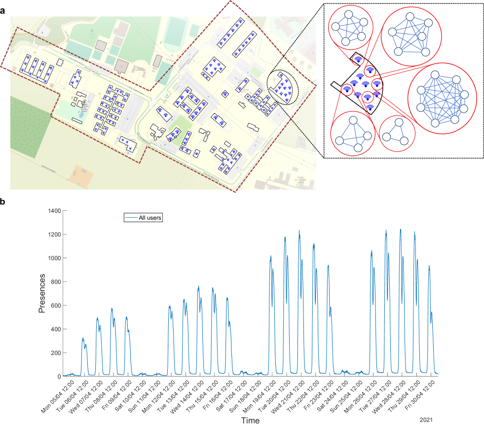
Figure 5: WIFI data for gatherings at University of Parma. a Map of the University of Parma Campus, called ”Parco Area delle Scienze”, where scientific departments are located with facilities for teaching and research activities (classrooms, laboratories, study spaces and libraries). The map highlights schematically the buildings where the gatherings are recorded through WIFI access points data. b Plot of the temporal dependence of the number of users connected to WIFI from 05th April 2021 to 30th April 2021. On Saturdays and Sundays the accesses were minimal, as well as on 05th April 2021 being Easter Monday (public holiday in Italy). A rapid increase in the number of users occurred in the morning, followed by a reduction in connections at lunchtime, a resumption in the afternoon and a dramatic decrease in the evening. The plot covers both partial opening and closure periods due to COVID-19 containment measures: from 05th April to 18th April (closure period) attendance was low, while from 19th April to 30th April (partial opening period) it increased significantly.

IV.2 Model parameters

Throughout the paper the parameter values are, unless specified otherwise, tailored to describe the SARS-CoV-2 diffusion. The probability for an individual to develop symptoms is $\delta=0.57$ [47]. The average time for the appearance of symptoms, i.e. the average time after which a presymptomatic individual spontaneously develops symptoms, is $\tau_{P}=1/\gamma_{P}=1.5$ days [41, 48]. The average recovery time is $\tau=1/\mu=14$ days [32, 49]. In order to implement all CT mechanisms, we assume contacts are reconstructed over $T_{CT}=\tau=14$ days, so that it is possible to track nodes infected by the index case in its presymptomatic phase (forward CT), the source of infection of the index case (backward CT) and all other infections occurred in simplicial interactions (sideward CT). The average number of daily contacts per individual is fixed to $\overline{n}=14$ [50, 33]. Notice that with these realistic values of the parameters, $R_{0}\approx 4.5$ corresponds to $\lambda\approx 0.02$. This implies that even in the largest gathering that we consider of about hundreds of nodes, at most only 10-20 individuals can be infected.

IV.3 WIFI data: preprocessing and main properties

Like many universities, the University of Parma has covered its buildings with a single WIFI network (see Fig. 5a), enabling users to establish more than 10000 sessions a day. All sessions data from the login management system are collected by the ”ICT services” office of Parma University. The login management system manages all wireless access points (APs) and all users’ requests for connection to the internet with their registered device. University WIFI users are all people with institutional account (students, professors, researchers and staff) and all people from other European Universities with an account for the EDUROAM network. It is possible to create temporary accounts for external guests.

The dataset refers to a sample of 713 wireless access points, about 10000 daily connections and spans six months, starting on 10th December 2020 and ending on 09th May 2021. During this period, due to the COVID-19 pandemic restrictions, we can distinguish two different phases: a closure phase and a partial opening phase [40].

• Closure phase. During this phase, the access to all University buildings was allowed only to authorised staff, professors, researchers and students only to participate in laboratory activities. All lectures were offered remotely on video-conferencing platforms. This phase spans the period from 10th December 2020 to 21st February 2021 and from 15th March 2021 to 18th April 2021. In this period the number of users is 7138;

• Partial opening phase. During this phase, the access to University buildings was extended to first year students attending in-person classes (about 25% students enrolled in the degree courses) while the lectures of all others students were offered remotely on video-conferencing platforms. Libraries and study spaces reopened with a reduction of rooms’ maximum capacity and mandatory reservation. This phase spans the period from 22nd February 2021 to 14th March 2021 and from 19th April 2021 to 09th May 2021. In this period the number of users is 7835;

We provided the ”ICT services” office with a script that extracts from the login management system the anonimysed aggregated data on the attendance at the University and its temporal dynamics (see SM). In Fig. 5b we plot the number of people present at the University as a function of time. Data show the reliability of the measure: the closure period up to the 18th of April and the following days of partial opening are clearly distinct on the plot; in the week-ends and on public holidays (April 5th) attendance is limited; during night hours connections are nearly absent and we also observe the effect of lunch breaks. The attendance estimated via WIFI data underestimates the true number of people simultaneously present, since not all individuals connect to the WIFI network. A reasonable estimate is that the number of people actually present is roughly twice as large. This assessment is based on the comparison of WIFI data with the number of seat reservations in classrooms and study rooms made by students (mandatory for University regulations [40]) and with the number of attending professors, researchers and university staff, as revealed by data from their personal badges.

IV.4 Empirical simplex size distribution from WIFI data

From the WIFI dataset of the University of Parma, we extract two different simplex size distributions: one for the closure phase and one for the partial opening phase. To control the signal noise of day-to-day random variations, we take the entire dataset and remove public holidays, weekends and the night time data (from 8:00 p.m. to 7:00 a.m.). We define as a simplex of size $s$ a group of $s$ users connected to the same AP for at least 15 minutes (the same time used in contact tracing apps to consider a contact epidemiologically significant and at high-risk [37]). For both phases, we reconstruct all connection sessions of all users, their location and their duration from the WIFI log file. It is possible that some connections are interrupted for various technical reasons (such as weak signal or the user’s device going in standby): to control for these effects, if a user connects twice to the same AP and the time lag $\Delta t$ between the two sessions is smaller than 5 minutes, we consider it as a single connection. To obtain all simplices activated inside the University we focus on connections to a given AP. We split working hours (from 7:00 a.m. to 8:00 p.m.) into 15 minutes intervals and for each interval we find the number of users that remained connected to the same AP for the full time interval: this number corresponds to the simplex size. This operation is repeated for every working day and for each AP. These data, separated for the two periods, determine the empirical simplex size distributions (Fig. 4a).

V Authors’ contributions

M.M., A.G., C.C., A.V. and R.B. designed research, M.M., A.G., C.C., A.V. and R.B. performed research, M.M. and A.G. analyzed data, M.M., A.G., C.C., A.V. and R.B. wrote the paper.

VI Competing interests

The authors declare no competing interests.

VII Acknowledgements

We warmly thank the Operative Unit ”Technological Systems and Infrastructures” of the University of Parma and in particular A. Barontini, F. Russo and C. Valenti for the constant support in data elaboration. We also thank M. Mamei for very useful discussions and suggestions.

VIII Funding

R.B., A.G. and A.V. acknowledge support from the EU-PON Project POR FSE Emilia Romagna 2018/2020 Objective 10.

References

- [1] Moghadas, S. M., Sah, P., Vilches, T. N. & Galvani, A. P., 2021 Can the usa return to pre-covid-19 normal by july 4? Lancet Infect. Dis. 21, 1073–1074. (doi:10.1016/S1473-3099(21)00324-8).
- [2] Di Domenico, L., Sabbatini, C. E., Boëlle, P.-Y., Poletto, C., Crépey, P., Paireau, J., Cauchemez, S., Beck, F., Noel, H., Lévy-Bruhl, D. et al., 2021 Adherence and sustainability of interventions informing optimal control against the covid-19 pandemic. Commun. Med. 1, 57. (doi:10.1038/s43856-021-00057-5).
- [3] Scott, N., Palmer, A., Delport, D., Abeysuriya, R., Stuart, R., Kerr, C. C., Mistry, D., Klein, D. J., Sacks-Davis, R., Heath, K. et al., 2020 Modelling the impact of reducing control measures on the covid-19 pandemic in a low transmission setting. medRxiv (doi:10.1101/2020.06.11.20127027).
- [4] Bonaccorsi, G., Pierri, F., Cinelli, M., Flori, A., Galeazzi, A., Porcelli, F., Schmidt, A. L., Valensise, C. M., Scala, A., Quattrociocchi, W. et al., 2020 Economic and social consequences of human mobility restrictions under covid-19. Proc. Natl. Acad. Sci. U.S.A. 117, 15530–15535. (doi:10.1073/pnas.2007658117).
- [5] Mandel, A. & Veetil, V., 2020 The economic cost of covid lockdowns: An out-of-equilibrium analysis. Econ. Dis. Cli. Cha. 4, 431–451. (doi:10.1007/s41885-020-00066-z).
- [6] McKee, M. & Stuckler, D., 2020 If the world fails to protect the economy, covid-19 will damage health not just now but also in the future. Nat. Med. 26, 640–642. (doi:10.1038/s41591-020-0863-y).
- [7] Chang, S., Pierson, E., Koh, P. W., Gerardin, J., Redbird, B., Grusky, D. & Leskovec, J., 2021 Mobility network models of covid-19 explain inequities and inform reopening. Nature 589, 82–87. (doi:10.1038/s41586-020-2923-3).
- [8] Moghadas, S. M., Fitzpatrick, M. C., Sah, P., Pandey, A., Shoukat, A., Singer, B. H. & Galvani, A. P., 2020 The implications of silent transmission for the control of covid-19 outbreaks. Proc. Natl. Acad. Sci. U.S.A. 117, 17513–17515. (doi:10.1073/pnas.2008373117).
- [9] Pullano, G., Di Domenico, L., Sabbatini, C. E., Valdano, E., Turbelin, C., Debin, M., Guerrisi, C., Kengne-Kuetche, C., Souty, C., Hanslik, T. et al., 2021 Underdetection of cases of covid-19 in france threatens epidemic control. Nature 590, 134–139. (doi:10.1038/s41586-020-03095-6).
- [10] Sekara, V., Stopczynski, A. & Lehmann, S., 2016 Fundamental structures of dynamic social networks. Proc. Natl. Acad. Sci. U.S.A. 113, 9977–9982. (doi:10.1073/pnas.1602803113).
- [11] Battiston, F., Cencetti, G., Iacopini, I., Latora, V., Lucas, M., Patania, A., Young, J.-G. & Petri, G., 2020 Networks beyond pairwise interactions: Structure and dynamics. Phys. Rep. 874, 1–92. (doi:10.1016/j.physrep.2020.05.004).
- [12] Cencetti, G., Battiston, F., Lepri, B. & Karsai, M., 2021 Temporal properties of higher-order interactions in social networks. Sci. Rep. 11, 7028. (doi:10.1038/s41598-021-86469-8).
- [13] Lewis, D., 2021 Superspreading drives the covid pandemic-and could help to tame it. Nature 590, 544–546. (doi:10.1038/d41586-021-00460-x).
- [14] Althouse, B. M., Wenger, E. A., Miller, J. C., Scarpino, S. V., Allard, A., Hébert-Dufresne, L. & Hu, H., 2020 Superspreading events in the transmission dynamics of sars-cov-2: Opportunities for interventions and control. PLOS Biol. 18, 1–13. (doi:10.1371/journal.pbio.3000897).
- [15] Adam, D. C., Wu, P., Wong, J. Y., Lau, E. H. Y., Tsang, T. K., Cauchemez, S., Leung, G. M. & Cowling, B. J., 2020 Clustering and superspreading potential of sars-cov-2 infections in hong kong. Nat. Med. 26, 1714–1719. (doi:10.1038/s41591-020-1092-0).
- [16] Majra, D., Benson, J., Pitts, J. & Stebbing, J., 2021 Sars-cov-2 (covid-19) superspreader events. J. Infect. 82, 36–40. (doi:10.1016/j.jinf.2020.11.021).
- [17] Iacopini, I., Petri, G., Barrat, A. & Latora, V., 2019 Simplicial models of social contagion. Nat. Commun. 10, 2485. (doi:10.1038/s41467-019-10431-6).
- [18] St-Onge, G., Thibeault, V., Allard, A., Dubé, L. J. & Hébert-Dufresne, L., 2021 Social confinement and mesoscopic localization of epidemics on networks. Phys. Rev. Lett. 126, 098301. (doi:10.1103/PhysRevLett.126.098301).
- [19] Fraser, C., Riley, S., Anderson, R. M. & Ferguson, N. M., 2004 Factors that make an infectious disease outbreak controllable. Proc. Natl. Acad. Sci. U.S.A. 101, 6146–6151. (doi:10.1073/pnas.0307506101).
- [20] Thompson, R. N., Gilligan, C. A. & Cunniffe, N. J., 2016 Detecting presymptomatic infection is necessary to forecast major epidemics in the earliest stages of infectious disease outbreaks. PLOS Comput. Biol. 12, 1–18. (doi:10.1371/journal.pcbi.1004836).
- [21] Pinotti, F., Di Domenico, L., Ortega, E., Mancastroppa, M., Pullano, G., Valdano, E., Boëlle, P.-Y., Poletto, C. & Colizza, V., 2020 Tracing and analysis of 288 early sars-cov-2 infections outside china: A modeling study. PLOS Med. 17, 1–13. (doi:10.1371/journal.pmed.1003193).
- [22] Johansson, M. A., Quandelacy, T. M., Kada, S., Prasad, P. V., Steele, M., Brooks, J. T., Slayton, R. B., Biggerstaff, M. & Butler, J. C., 2021 SARS-CoV-2 Transmission From People Without COVID-19 Symptoms. JAMA Netw. Open 4, e2035057–e2035057. (doi:10.1001/jamanetworkopen.2020.35057).
- [23] Kojaku, S., Hébert-Dufresne, L., Mones, E., Lehmann, S. & Ahn, Y.-Y., 2021 The effectiveness of backward contact tracing in networks. Nat. Phys. 17, 652–658. (doi:10.1038/s41567-021-01187-2).
- [24] Bradshaw, W. J., Alley, E. C., Huggins, J. H., Lloyd, A. L. & Esvelt, K. M., 2021 Bidirectional contact tracing could dramatically improve covid-19 control. Nat. Commun. 12, 232. (doi:10.1038/s41467-020-20325-7).
- [25] Endo, A., CMMID COVID-19 Working Group, Leclerc, Q. J., Knight, G. M., Medley, G. F., Atkins, K. E., Funk, S. & Kucharski, A. J., 2020 Implication of backward contact tracing in the presence of overdispersed transmission in covid-19 outbreaks. Wellcome Open Res. 5, 239. (doi:10.12688/wellcomeopenres.16344.3).
- [26] Petri, G. & Barrat, A., 2018 Simplicial activity driven model. Phys. Rev. Lett. 121, 228301. (doi:10.1103/PhysRevLett.121.228301).
- [27] Holme, P. & Saramäki, J., 2019 Temporal Network Theory. Cham, Switzerland: Springer. (doi:10.1007/978-3-030-23495-9).
- [28] Perra, N., Gonçalves, B., Pastor-Satorras, R. & Vespignani, A., 2012 Activity driven modeling of time varying networks. Sci. Rep. 2, 469. (doi:10.1038/srep00469).
- [29] Ubaldi, E., Perra, N., Karsai, M., Vezzani, A., Burioni, R. & Vespignani, A., 2016 Asymptotic theory of time-varying social networks with heterogeneous activity and tie allocation. Sci. Rep. 6, 35724. (doi:10.1038/srep35724).
- [30] Mancastroppa, M., Vezzani, A., Muñoz, M. A. & Burioni, R., 2019 Burstiness in activity-driven networks and the epidemic threshold. J. Stat. Mech. Theory Exp. 2019, 053502. (doi:10.1088/1742-5468/ab16c4).
- [31] Guan, W.-j., Ni, Z.-y., Hu, Y., Liang, W.-h., Ou, C.-q., He, J.-x., Liu, L., Shan, H., Lei, C.-l., Hui, D. S. et al., 2020 Clinical characteristics of coronavirus disease 2019 in china. N. Engl. J. Med. 382, 1708–1720. (doi:10.1056/NEJMoa2002032).
- [32] World Health Organization, 2020. Report of the who-china joint mission on coronavirus disease 2019 (covid-19). https://www.who.int/docs/default-source/coronaviruse/who-china-joint-mission-on-covid-19-final-report.pdf. Accessed on: 05-01-2022.
- [33] Van Kerckhove, K., Hens, N., Edmunds, W. J. & Eames, K. T. D., 2013 The Impact of Illness on Social Networks: Implications for Transmission and Control of Influenza. Am. J. Epidemiol. 178, 1655–1662. (doi:10.1093/aje/kwt196).
- [34] Pozzana, I., Sun, K. & Perra, N., 2017 Epidemic spreading on activity-driven networks with attractiveness. Phys. Rev. E 96, 042310. (doi:10.1103/PhysRevE.96.042310).
- [35] Mancastroppa, M., Burioni, R., Colizza, V. & Vezzani, A., 2020 Active and inactive quarantine in epidemic spreading on adaptive activity-driven networks. Phys. Rev. E 102, 020301. (doi:10.1103/PhysRevE.102.020301).
- [36] Mancastroppa, M., Castellano, C., Vezzani, A. & Burioni, R., 2021 Stochastic sampling effects favor manual over digital contact tracing. Nat. Commun. 12, 1919. (doi:10.1038/s41467-021-22082-7).
-
[37]
European Center for Disease Prevention and Control, 2021.
Mobile applications in support of contact tracing for covid-19.
https://www.ecdc.europa.eu/sites/default/files/documents/
covid-19-mobile-applications-contact-tracing.pdf. Accessed on: 05-01-2022. - [38] González-Cabañas, J., Cuevas, A., Cuevas, R. & Maier, M., 2021 Digital contact tracing: Large-scale geolocation data as an alternative to bluetooth-based apps failure. Electronics 10, 1093. (doi:10.3390/electronics10091093).
- [39] Cobb, S. M., 2020 Harvard to track affiliates’ wi-fi signals as part of contact tracing pilot. The Harvard Crimson Published on: 02-08-2020.
- [40] University of Parma, 2020. Coronavirus: all information for the university community updated in real time. https://www.unipr.it/coronavirus. Accessed on: 17-07-2021.
- [41] Di Domenico, L., Pullano, G., Sabbatini, C. E., Boëlle, P.-Y. & Colizza, V., 2020 Impact of lockdown on covid-19 epidemic in île-de-france and possible exit strategies. BMC Med. 18, 240. (doi:10.1186/s12916-020-01698-4).
- [42] World Health Organization, 2021. Tracking sars-cov-2 variants. https://www.who.int/en/activities/tracking-SARS-CoV-2-variants/. Accessed on: 05-01-2022.
- [43] Davies, N. G., Abbott, S., Barnard, R. C., Jarvis, C. I., Kucharski, A. J., Munday, J. D., Pearson, C. A. B., Russell, T. W., Tully, D. C., Washburne, A. D. et al., 2021 Estimated transmissibility and impact of sars-cov-2 lineage b.1.1.7 in england. Science 372. (doi:10.1126/science.abg3055).
- [44] Volz, E., Mishra, S., Chand, M., Barrett, J. C., Johnson, R., Geidelberg, L., Hinsley, W. R., Laydon, D. J., Dabrera, G., O’Toole, Á. et al., 2021 Assessing transmissibility of sars-cov-2 lineage b.1.1.7 in england. Nature 593, 266–269. (doi:10.1038/s41586-021-03470-x).
- [45] Sonabend, R., Whittles, L. K., Imai, N., Knock, E. S., Perez-Guzman, P. N., Rawson, T., Mangal, T., Volz, E. M., Ferguson, N. M., Baguelin, M. et al., 2021. Evaluating the roadmap out of lockdown: modelling step 4 of the roadmap in the context of b.1.617.2. https://www.gov.uk/government/publications/imperial-college-london-evaluating-the-roadmap-out-of-lockdown-modelling-step-4-of-the-roadmap-in-the-context-of-b16172-delta-9-june-2021. Accessed on: 05-01-2022.
- [46] Tizzani, M., Lenti, S., Ubaldi, E., Vezzani, A., Castellano, C. & Burioni, R., 2018 Epidemic spreading and aging in temporal networks with memory. Phys. Rev. E 98, 062315. (doi:10.1103/PhysRevE.98.062315).
- [47] Lavezzo, E., Franchin, E., Ciavarella, C., Cuomo-Dannenburg, G., Barzon, L., Del Vecchio, C., Rossi, L., Manganelli, R., Loregian, A., Navarin, N. et al., 2020 Suppression of a sars-cov-2 outbreak in the italian municipality of vo’. Nature 584, 425–429. (doi:10.1038/s41586-020-2488-1).
- [48] Wei, W. E., Li, Z., Chiew, C. J., Yong, S. E., Toh, M. P. & Lee, V. J., 2020 Presymptomatic transmission of sars-cov-2—singapore, january 23–march 16, 2020. Morb. Mortal. Wkly. Rep. 69, 411. (doi:10.15585/mmwr.mm6914e1).
- [49] Liu, Y., Yan, L.-M., Wan, L., Xiang, T.-X., Le, A., Liu, J.-M., Peiris, M., Poon, L. L. & Zhang, W., 2020 Viral dynamics in mild and severe cases of covid-19. Lancet Infect. Dis. 20, 656–657. (doi:10.1016/S1473-3099(20)30232-2).
- [50] Mossong, J., Hens, N., Jit, M., Beutels, P., Auranen, K., Mikolajczyk, R., Massari, M., Salmaso, S., Tomba, G. S., Wallinga, J. et al., 2008 Social contacts and mixing patterns relevant to the spread of infectious diseases. PLOS Med. 5, 1–1. (doi:10.1371/journal.pmed.0050074).