Ordinary Differential Equation Models and their Computation Methods

Abstract

In this article, I introduce the differential equation model and review their frequentist and Bayesian computation methods. A numerical example of the FitzHugh-Nagumo model is given.

1 Introduction

I spent a Sabbatical year in the Statistical and Applied Mathematical Sciences Institute in 2010. During the Sabbatical year, I attended a talk given by James Ramsay. He gave a talk on the differential equation model and an example of modeling underground water levels in some place in Canada. The water level data can be seen as a function of time and its plot was not smooth at all. It was wiggly and has big jumps. The water level was mostly affected by the rainfall, but with some time lags. He showed the fitted curves and predictions. I was very surprised that his fitted curve as well as the predictions follow the observed data very closely. I would not be surprised by the fitted curve following the data closely if the model has thousands of parameters, but his estimate follows the data with just a handful of parameters. At the talk I imagined myself analyzing the same data set without the differential equation model. I thought about many complicated nonparametric models, but I could not think of a statistical model which would resemble the fitted curve he produce on his slide. This is how I got drawn to the topic of the differential equation model.

The differential equation is a primary mathematical model that describes dynamical systems which are first developed by Henri Poincaré to explain celestial bodies. Differential equations are widely used in many different areas such as the epidemic model, climate model, economic model, and chemical engineering, to name just a few. The statistics community however largely neglected the differential equation modeling until recently.

The differential equation model is a statistical model that consists of two equations:

observation equation: $$\displaystyle y(t_{i}) \displaystyle=x(t_{i})+\epsilon(t_{i}),~{}i=1,2,\ldots,n,$$ (1)

differential equation: $$\displaystyle\frac{dx(t)}{dt} \displaystyle=f(x(t),t;\theta),$$ (2)

where $\displaystyle 0<t_{1}<t_{2}<\ldots<t_{n}<T$ are time points where observations $\displaystyle y(t)$ are observed and $\displaystyle\epsilon(t_{i})$’s are observational error typically assumed to follow $\displaystyle N(0,\Sigma)$ with positive definite matrix $\displaystyle\Sigma$. The error variance $\displaystyle\Sigma$ is assume typically a diagonal matrix $\displaystyle\Sigma=diag(\sigma_{1}^{2},\ldots,\sigma_{p}^{2})$. Here $\displaystyle y(t)$ is a $\displaystyle p$-dimensional vector that are observable and $\displaystyle x(t)$ is also a $\displaystyle p$-dimensional vector function that satisfies the differential equation (2) and it is the mean function of the regression model (1). The function $\displaystyle f$ is smooth and uniquely determines $\displaystyle x$ when the initial value of $\displaystyle x$, $\displaystyle x_{0}=x(0)$ is given. Note that the differential equation model (1) and (2) is just a nonlinear regression model where the mean function of the regression model is expressed as a solution of a differential equation. It also resembles the state-space model. One can view that the differential equation model as the state-space model whose state equation is expressed as a differential equation.

Here I give an example of the differential equation model. The SIR model is the differential equation model for disease spread in a small community. It consists of differential equations for three curves, susceptible (S), infected (I), and recovered (R):

$$\displaystyle\frac{dS(t)}{dt} \displaystyle= \displaystyle-\beta\frac{1}{N}I(t)S(t)$$

$$\displaystyle\frac{dI(t)}{dt} \displaystyle= \displaystyle\beta\frac{1}{N}I(t)S(t)-\gamma I(t)$$

$$\displaystyle\frac{dR(t)}{dt} \displaystyle= \displaystyle\gamma I(t),$$

where $\displaystyle t$ is time in $\displaystyle[0,T]$, for some $\displaystyle T>0$, $\displaystyle N$ is the total population of the community, and $\displaystyle S(t)$, $\displaystyle I(t)$ and $\displaystyle R(t)$ are the numbers of the susceptibles, the infected and the recovered at time $\displaystyle t$, respectively. There are three equations in the model, but fundamental quantities are two terms. One is $\displaystyle\beta\frac{1}{N}I(t)S(t)$ which can be interpreted as the number of infected people in a unit time. The parameter $\displaystyle\beta^{\prime}=\beta/N$ is the probability that one infected and one susceptible meet and the susceptible gets infected during a unit time and $\displaystyle\beta$ is the number of people in the population or among $\displaystyle N$ susceptibles who get infected by one infected during a unit time. Some authors prefer $\displaystyle\beta^{\prime}$ and use

$$\frac{dS(t)}{dt}=-\beta^{\prime}I(t)S(t).$$

Another fundamental quantity is $\displaystyle\gamma I(t)$ which is the number of recovered during a unit time. The parameter $\displaystyle\gamma$ is the recovery rate of the infected during a unit time. For the SIR model, we assume the population size $\displaystyle N$ remains constant over the time period $\displaystyle[0,T]$ and

$$S(t)+I(t)+R(t)=N,~{}\forall t.$$

Thus, essentially we need only two equations.

In the differential equation model, we assume that we do not observe $\displaystyle S(t)$, $\displaystyle I(t)$ and $\displaystyle R(t)$ directly, but observe them with errors, i.e. we observe $\displaystyle S^{*}(t_{i})$ and $\displaystyle I^{*}(t_{i})$ at $\displaystyle 0<t_{1}<t_{2}<\ldots<t_{n}<T$:

$$\displaystyle S^{*}(t_{i}) \displaystyle= \displaystyle S(t_{i})+\epsilon_{1}(t_{i}),$$

$$\displaystyle I^{*}(t_{i}) \displaystyle= \displaystyle I(t_{i})+\epsilon_{2}(t_{i}),$$

where $\displaystyle\epsilon_{1}(t)$ and $\displaystyle\epsilon_{2}(t)$ are errors.

This article is organized as follows. In sections 2 and 3, frequentist and Bayesian methods in the literature are reviewed, respectively. In section 3, a numerical example of the FitzHugh-Nagumo model is given.

2 Frequentist Methods

2.1 Explicit Numerical Integration of Differential Equation

bard1974nonlinear considers in his book the parameter estimation of the dynamic model with errors. The parameter of the differential equation is estimated with the least squares method, i.e.,

$$\hat{\theta}:=argmin_{\theta}||y_{i}-x(t_{i})||^{2}.$$

In the course of the optimization, whenever a value of $\displaystyle x(t)$ is required, a numerical solver is invoked.

This method performs well when the sample size and the number of parameters are small. But its computation can be prohibitive when the model gets larger. When the numerical solver is the 4th order Runge-Kutta algorithm, the estimator is asymptotically efficient (Xue et al. 2010, Bhaumik and Ghosal 2017).

2.2 Two-step methods

varah1982spline proposed the two-step method. In the first step, $\displaystyle x(t)$ is estimated with a cubic spline with fixed knots using the observed data $\displaystyle\mathbf{y}=(y(t_{1}),\ldots,y(t_{n}))$ without considering the differential equation. In the second step, $\displaystyle\theta$ is obtained by minimizing the distance between the estimated $\displaystyle\frac{d\hat{x}(t)}{dt}$ and $\displaystyle f(\hat{x}(t),t,\theta)$, i.e.,

$$\hat{\theta}:=argmin_{\theta}\sum_{i=1}^{n}||\frac{d\hat{x}(t_{i})}{dt}-f(\hat{x}(t_{i}),t_{i},\theta)||^{2}.$$ (3)

There are variations in the first and the second steps with different nonparametric function estimation methods and different norms. This method is not asymptotically efficient but computationally fast.

2.3 Iterated Principal Differential Analysis

ramsay2005functional considered a variation of two-step method. In the proposed method, the following two steps are iterated.

In the first step, the cubic spline with fixed knots is fitted but with a penalty term, i.e.,

$$\hat{x}=argmin_{x}\sum_{i=1}^{n}||y_{i}-x(t_{i})||^{2}+\lambda\int(\dot{x}(t)-f(x,t,\theta))^{2}dt,$$

where $\displaystyle\theta$ is the estimated value in the previous iteration. In the second step, $\displaystyle\theta$ is obtained by minimizing (3).

2.4 Generalized Profiling Method

ramsay2007parameter proposed the generalized profiling method. They grouped the parameters in three groups, regularization parameter $\displaystyle\lambda$, the parameter in the differential equation $\displaystyle\theta$ and $\displaystyle\sigma$’s, and regression coefficients $\displaystyle\beta$ of basis expansion of x. Each group is estimated and thus eliminated in turn in three steps.

In the first step, $\displaystyle\lambda$ is estimated by a generalized cross-validation criterion. In the first step, whenever one needs values of $\displaystyle\theta$, $\displaystyle\sigma$’s and $\displaystyle\beta$, one evaluate them in the following second and third step. In the second step, $\displaystyle\theta(\lambda)$ is estimated by minimizing

$$\hat{\theta}(\lambda):=argmin_{\theta}||y_{i}-x(t_{i})||^{2}$$

where $\displaystyle x(t)=\beta^{\prime}b(t)$, $\displaystyle b(t)=(b_{1}(t),\ldots,b_{k}(t))$ and $\displaystyle b_{j}(t)$ are the B-spline basis. In the third step, $\displaystyle\beta(\lambda,\theta)$ is estimated by minimizing

$$\sum_{i=1}^{n}||y_{i}-x(t_{i})||^{2}+\lambda\int(\dot{x}(t)-f(x,t,\theta))^{2}dt,$$

where $\displaystyle\dot{x}(t)=\beta^{\prime}\dot{b}(t)$. In the above description, $\displaystyle\theta(\lambda)$ and $\displaystyle\beta(\lambda,\theta)$ are used to emphasize the dependence to $\displaystyle\lambda$, and $\displaystyle\lambda$ and $\displaystyle\theta$, respectively, The generalized profiling estimator is asymptotically efficient [qi2010asymptotic].

3 Bayesian Methods

In this section, the Bayesian estimation methods for the differential equation model are reviewed. There are three groups of parameters in the differential equation model. Two are obvious and one is not. The two groups of obvious parameters are the parameter in the differential equation (2), $\displaystyle\theta$, and the observational error variance $\displaystyle\Sigma$. Under some smoothness conditions, the differential equation together with initial value of $\displaystyle x$, $\displaystyle x_{0}:=x(0)$, uniquely determine $\displaystyle x$. Thus, one needs to include the initial value of $\displaystyle x$, $\displaystyle x_{0}:=x(0)$, which is not so obvious at a glance. To complete the Bayesian model, we need to put a prior on $\displaystyle\theta,\Sigma$ and $\displaystyle x_{0}$. We will denote the prior

$$(\theta,\boldsymbol{\sigma}^{2},x_{0})\sim\pi(\theta)\pi(\boldsymbol{\sigma})\pi(x_{0}).$$

3.1 Bayesian Method with Explicit Integration of Differential Equation

The first approach was the approach taken in gelman1996physiological. The posterior is

$$\pi(\theta,\boldsymbol{\sigma}^{2},x_{0}|\mathbf{y},\mathbf{x})\propto\pi(\theta,\boldsymbol{\sigma}^{2},x_{0})\times p(\mathbf{y}|\mathbf{x},\boldsymbol{\sigma},x_{0}),$$

where

$$p(\mathbf{y}|\mathbf{x},\boldsymbol{\sigma},x_{0})=\prod_{i=1}^{n}|2\pi\Sigma|^{-\frac{1}{2}}e^{-\frac{1}{2}(y_{i}-x(t_{i};\theta,x_{0}))^{\prime}\Sigma^{-1}(y_{i}-x(t_{i};\theta,x_{0}))},$$

$\displaystyle x(t)$ is denoted as $\displaystyle x(t;\theta,x_{0})$ to show the dependence on $\displaystyle\theta$ and $\displaystyle x_{0}$, $\displaystyle\mathbf{x}=(x(t_{1}),\ldots,x(t_{n}))$, $\displaystyle\mathbf{y}=(y(t_{1}),y(t_{2}),\ldots,y(t_{n}))$ and $\displaystyle\boldsymbol{\sigma}=(\sigma_{1},\sigma_{2},\ldots,\sigma_{p})$. To compute the posterior, one can apply the Markov chain Monte Carlo algorithm such as Metropolis-Hastings sampler or Hamiltonian Monte Carlo. The advantage of this method is that it computes the exact posterior while other methods employ certain approximations to ease the posterior computation. The difficulties with this approach are twofold. First, the analytic solution of the differential equation (2) is typically not available and whenever you need the likelihood, you need to resort to a numerical solver of the differential equation. This makes the posterior computation intensive. Second, the differential equation can be chaotic and a small variation in the parameter may result in completely different curves. Thus, estimation of the parameter can be very sensitive and it affects at times poor performances of the estimator.

dass2017laplace used the Laplace approximation method to speed up the posterior computation in which the function $\displaystyle x$ is evaluated using mathematical formulas of the Euler method or the 4th order Runge-Kutta method. This method gives accurate parameter estimates with fast computing time with a moderate dimension sizes of $\displaystyle\theta$. But when the dimension of $\displaystyle\theta$ is high, the computation can be intensive.

bhaumik2017efficient proved the Bernstein-von Mises theorem and the posterior is asymptotically efficient when the numerical solver is the 4th order Runge-Kutta.

3.2 Bayesian Collocation Method

campbell2012smooth use a Bayesian approach based on the collocation method and a prior on $\displaystyle x(t)$ was based on the penalty. The collocation approach is to express $\displaystyle x$ with a linear combination of bases, i.e.,

$$x(t)=\sum_{j=1}^{k}\beta_{j}b_{j}(t),$$

where $\displaystyle b_{j}(t)$’s are bases of function spaces, e.g. spline bases. The model can be viewed as

$$y(t_{i})=x(t_{i})+\epsilon(t_{i}),~{}\epsilon(t_{i})\stackrel{{\scriptstyle i.i.d.}}{{\sim}}N(0,\sigma^{2}),~{}i=1,2,\ldots,n$$

and $\displaystyle\frac{dx}{dt}=\dot{x}$ has prior

$$exp[-\lambda PEN(x)],$$

where

$$PEN(x)=\int||\frac{dx}{dt}-f(x(t),t,u(t);\theta)||^{2}dt.$$

Thus, the posterior is

$$\pi(\theta,\sigma^{2},\alpha)\propto e^{-\lambda PEN(x;\alpha,\theta)}\times p(\mathbf{y}|\mathbf{x},\boldsymbol{\sigma},x_{0}).$$

The approach taken by campbell2012smooth is slightly more complicated than the above and used tempering idea with different $\displaystyle\lambda$s.

3.3 Gaussain Process Approaches

The key fact used in the Gaussian process approach is the fact that when $\displaystyle x$ follows a Gaussian process, $\displaystyle x$ and $\displaystyle\dot{x}$ are jointly a Gaussian process. This contradicts the mathematical fact that when $\displaystyle x$ is a function, $\displaystyle x$ determines $\displaystyle\dot{x}$. Nevertheless, it gives a methodological advantage in ordinary differential equation (ODE) models. There are two approaches in this category: adaptive gradient matching (AGM) method (Calderhead et al. 2009; Dondelinger et al. 2013) and Gaussian process ODE (GPODE) method [wang2014gaussian].

Suppose $\displaystyle x\sim GP(0,C_{\phi})$, the Gaussian process with mean function $\displaystyle 0$ and covariance function $\displaystyle C_{\phi}$ with parameter $\displaystyle\phi$. In the AGM method, the posterior is obtained by

$$\pi(\theta,\boldsymbol{\sigma},\phi|\mathbf{x},\mathbf{y})\propto p(\mathbf{y}|\mathbf{x},\boldsymbol{\sigma},x_{0})\times\pi(x|\theta,\phi,\gamma)\times\pi(\theta,\phi,\gamma,\boldsymbol{\sigma}),$$

where $\displaystyle\pi(\theta,\phi,\gamma,\boldsymbol{\sigma})$ is the prior $\displaystyle(\theta,\phi,\gamma,\boldsymbol{\sigma})$ and $\displaystyle\gamma$ is the additional error variance introduced to $\displaystyle\dot{x}$ in (6). The prior $\displaystyle\pi(x|\theta,\phi,\gamma)$ is constructed by

$$\pi(x|\theta,\phi,\gamma)=\int\pi(x,\dot{x}|\theta,\phi,\gamma)d\dot{x}$$ (4)

where

$$\pi(x,\dot{x}|\theta,\phi,\gamma)\propto GP(x,|0,C_{\phi})GP(\dot{x}|x,\phi)\prod_{i=1}^{n}N(\dot{x}(t_{i})|f(t_{i},x(t_{i}),\theta),\gamma I).$$ (5)

Note that integration (4) can be performed explicitly. In (5), the second factor $\displaystyle GP(\dot{x}|x,\phi)$ of the right hand side is derived from the assumption that $\displaystyle x$ follows a Gaussian process and the third factor by relaxing differential equation (2) with

$$\dot{x}(t_{i})=f(x(t_{i}),t_{i};\theta)+\nu_{i},~{}\nu_{i}\stackrel{{\scriptstyle i.i.d.}}{{\sim}}N(0,\gamma).$$ (6)

Note that this is not a legitimate derivation following probability laws, because the distributions of $\displaystyle\dot{x}$ from two sources are multiplied.

In the GPODE method, the posterior is obtained as

$$\pi(\theta,\phi,\boldsymbol{\sigma}|\mathbf{y},\mathbf{x})\propto p(\mathbf{y}|\mathbf{f},\phi,\boldsymbol{\sigma})\times GP(x|0,C_{\phi}),$$

where $\displaystyle\mathbf{f}=(f(t_{i},x(t_{i}),\theta))_{i=1}^{n}$ and $\displaystyle p(\mathbf{y}|\mathbf{f},\phi,\boldsymbol{\sigma})$ is $\displaystyle p(\mathbf{y}|\dot{\mathbf{x}},\phi,\boldsymbol{\sigma})$ with $\displaystyle\dot{\mathbf{x}}$ replaced by $\displaystyle\mathbf{f}$ using the differential equation. The conditional distribution $\displaystyle p(\mathbf{y}|\dot{\mathbf{x}},\phi,\boldsymbol{\sigma})$ is obtained by

$$p(\mathbf{y}|\dot{\mathbf{x}},\phi,\boldsymbol{\sigma})=\int p(\mathbf{y}|\dot{\mathbf{x}},\phi,\boldsymbol{\sigma})\times GP(\mathbf{x}|\dot{\mathbf{x}},\phi)d\mathbf{x}.$$

Conveniently, this integration also can be done explicitly under the normal error assumption.

3.4 Two-Step Approaches

bhaumik2015bayesian considered two step approach to the posterior computation of the ODE model. In the first step, the regression function $\displaystyle x$ is estimated without considering the differential equation using nonparametric Bayesian model with the B-spline basis

$$y_{j}=x(t_{j})+\epsilon(t_{j}),j=1,2,\ldots,n$$

where $\displaystyle x(t)=\sum_{j=1}^{k}\beta_{j}b_{j}(t)$, $\displaystyle b_{j}(t)$ are the B-spline basis and $\displaystyle\beta_{j}$ are coefficients of the basis. As a result of the first step, the posterior of $\displaystyle x(t)$ or $\displaystyle\beta_{j}$’s are obtained.

In the second step, one sample $\displaystyle\dot{x}$ from the posterior of $\displaystyle x$. Since the derivatives of the B-spline basis are well-known, one first samples $\displaystyle x$ from the posterior and can compute $\displaystyle\dot{x}$ analytically. For each sample of $\displaystyle\dot{x}$, one finds the matched $\displaystyle\theta$ by minimizing

$$\theta^{*}:=argmin_{\theta}\int||\dot{x}(t)-f(x(t),\theta)||^{2}w(t)dt$$

where $\displaystyle w(t)$ is a weight function. The posterior of $\displaystyle\theta$ is approximated by collecting $\displaystyle\theta^{*}$’s. bhaumik2015bayesian proved the posterior satisfies the Bernstein-von Mises theorem.

Two step approaches are not generally asymptotically efficient. But bhaumik2017efficient considered the second step where the posterior sample $\displaystyle\theta^{*}$ is obtained by matching the Runge-Kutta numerical solution as follows:

$$\theta^{*}:=argmin_{\theta}\int||x(t)-x^{*}_{\theta}(t)||^{2}dt,$$

where $\displaystyle x(t)$ is the posterior sample from the first step and $\displaystyle x^{*}_{\theta}(t)$ is the solution of the Runge-Kutta method with parameter $\displaystyle\theta$. They proved that the Bayes estimator from this posterior is asymptotically efficient.

3.5 Nonlinear State-Space Model Approximation

The relaxed differential equation model (RDEM) [lee2018inference] approximated the differential equation model (2), and the differential equation model is approximated by the nonlinear state-space model

$$\displaystyle y_{i} \displaystyle= \displaystyle x_{i}+\epsilon_{i},~{}\epsilon_{i}\stackrel{{\scriptstyle i.i.d.}}{{\sim}}N(0,\Sigma)$$ (7)

$$\displaystyle x_{i} \displaystyle= \displaystyle g(x_{i-1},t_{i-1};\theta)+\eta_{i},~{}\eta_{i}\stackrel{{\scriptstyle i.i.d.}}{{\sim}}N(0,V),~{}i=1,\ldots,n,$$ (8)

where

$$\displaystyle g(x_{i},t_{i};\theta) \displaystyle= \displaystyle x_{i}+{h_{i+1}\over 6}(k_{i1}+2k_{i2}+2k_{i3}+k_{i4})$$

$$\displaystyle k_{i1} \displaystyle= \displaystyle f(x_{i},t_{i};\theta),$$

$$\displaystyle k_{i2} \displaystyle= \displaystyle f(x_{i}+{h_{i+1}\over 2}k_{i1},t_{i}+{h_{i+1}\over 2};\theta),$$

$$\displaystyle k_{i3} \displaystyle= \displaystyle f(x_{i}+{h_{i+1}\over 2}k_{i2},t_{i}+{h_{i+1}\over 2};\theta),$$

$$\displaystyle k_{i4} \displaystyle= \displaystyle f(x_{i}+k_{i3},t_{i}+h_{i+1};\theta)$$

and $\displaystyle h_{i+1}=t_{i+1}-t_{i}$. Note that $\displaystyle g(x_{i},t_{i};\theta)$ in (8) is the equation of the 4th order Runge-Kutta method.

The posterior computation is done by a sequential Monte Carlo Method, the extended Liu and West filter [rios2013extended] in which $\displaystyle x_{i}$ is further relaxed with added noises. In the numerical experiments, RDEM saves the computation time drastically while the accuracy is comparable to the other methods.

The SSVB (state-space model with variational Bayes) [yang2021variational] applies the variational Bayes method to obtain the posterior of (8) and (8). yang2021variational considered the Lorenz-96 model [lorenz1995predictability] with $\displaystyle p=10$ variables as a numerical testbed:

$$\frac{dX_{j}}{dt}=(X_{j+1}-X_{j-2})X_{j-1}-X_{j}+F,\qquad\text{for }\ j=1,\ \dots,\ p,$$

and according to the circular structure, $\displaystyle X_{-1}=X_{p-1}$, $\displaystyle X_{0}=X_{p}$, and $\displaystyle X_{p+1}=X_{1}$. The Lorenz-96 model is a nice numerical testbed for the differential equation model, for it can be expanded as desired by increasing $\displaystyle p$. For the Lorenz-96 model with $\displaystyle 10$ variables, none of the competitors can estimate the true parameters reasonably while the SSVB performed reasonably well.

The SSVB is computationally fast and gives numerically stable estimates, but inherits the lack of variance estimates from the variational method. yang2021laplace proposed to estimate the variance of the posterior using the Laplace method.

4 FitzHugh-Nagumo Model

The FitzHugh-Nagumo model (FitzHugh, 1961; Nagumo et al. 1962) describes the action of spike potential in the giant axon of squid neurons by an ODE with two state variables and three parameters:

$$\displaystyle\dot{x}_{1}(t) \displaystyle= \displaystyle\theta_{3}\left(x_{1}(t)-\frac{1}{3}x_{1}^{3}(t)+x_{2}(t)\right),$$

$$\displaystyle\dot{x}_{2}(t) \displaystyle= \displaystyle-\frac{1}{\theta_{3}}\Big{(}x_{1}(t)-\theta_{1}+\theta_{2}x_{2}(t)\Big{)},$$

where $\displaystyle-0.8<\theta_{1},\theta_{2}<0.8$ and $\displaystyle 0<\theta_{3}<8$. The two state variables, $\displaystyle x_{1}(t)$ and $\displaystyle x_{2}(t)$, are the voltage across an membrane and outward currents at time $\displaystyle t$, respectively.

The data are generated from the differential equation model with the differential equation being the FitzHugh-Nagumo model and the fitted curves are given in Figure 1. In this particular example, the RDEM of dass2017laplace is used. The solid lines are $\displaystyle x_{1}(t)$ and $\displaystyle x_{2}(t)$ as a function of time from the FitzHugh-Nagumo model with $\displaystyle x(t_{0})=(-1,1)^{T},\theta=(0.2,0.2,3)^{T}$. The star-shaped points are the generated data of the populations with $\displaystyle\sigma^{2}=0.25$. The upper, lower and middle dotted lines are the 95 and 5 % quantiles and median of the posterior $\displaystyle\pi(x_{i}\mid\mathbf{y})$, respectively.

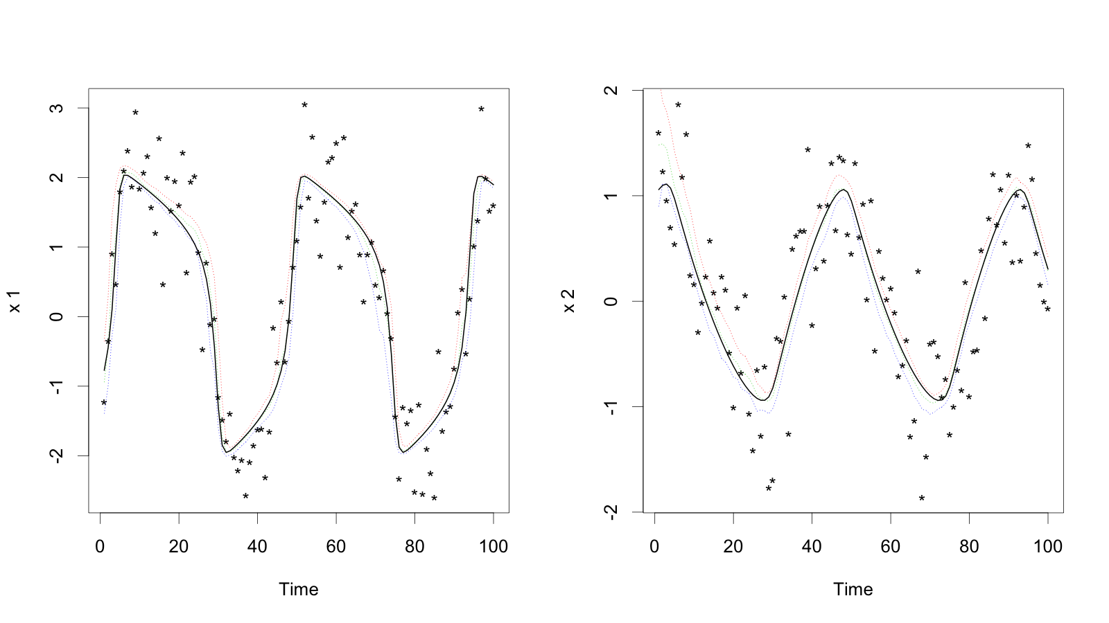
Figure 1: True and estimated curves of FitzHugh-Nagumo model.

References

- [1] \harvarditemBard1974bard1974nonlinear Bard, Y. \harvardyearleft1974\harvardyearright. Nonlinear parameter estimation, Academic Press.
- [2] \harvarditemBhaumik \harvardand Ghosal2015bhaumik2015bayesian Bhaumik, P. \harvardand Ghosal, S. \harvardyearleft2015\harvardyearright. Bayesian two-step estimation in differential equation models, Electronic Journal of Statistics 9(2): 3124–3154.
- [3] \harvarditemBhaumik \harvardand Ghosal2017bhaumik2017efficient Bhaumik, P. \harvardand Ghosal, S. \harvardyearleft2017\harvardyearright. Efficient bayesian estimation and uncertainty quantification in ordinary differential equation models, Bernoulli 23(4B): 3537–3570.
- [4] \harvarditem[Calderhead et al.]Calderhead, Girolami \harvardand Lawrence2008calderhead2008accelerating Calderhead, B., Girolami, M. \harvardand Lawrence, N. D. \harvardyearleft2008\harvardyearright. Accelerating bayesian inference over nonlinear differential equations with gaussian processes, Proceedings of the 21st International Conference on Neural Information Processing Systems, NIPS’08, Curran Associates Inc., Red Hook, NY, USA, p. 217–224.
- [5] \harvarditemCampbell \harvardand Steele2012campbell2012smooth Campbell, D. \harvardand Steele, R. J. \harvardyearleft2012\harvardyearright. Smooth functional tempering for nonlinear differential equation models, Statistics and Computing 22(2): 429–443.
- [6] \harvarditem[Dass et al.]Dass, Lee, Lee \harvardand Park2017dass2017laplace Dass, S. C., Lee, J., Lee, K. \harvardand Park, J. \harvardyearleft2017\harvardyearright. Laplace based approximate posterior inference for differential equation models, Statistics and Computing 27(3): 679–698.
- [7] \harvarditem[Dondelinger et al.]Dondelinger, Husmeier, Rogers \harvardand Filippone2013dondelinger2013ODE Dondelinger, F., Husmeier, D., Rogers, S. \harvardand Filippone, M. \harvardyearleft2013\harvardyearright. Ode parameter inference using adaptive gradient matching with gaussian processes, in C. M. Carvalho \harvardand P. Ravikumar (eds), Proceedings of the Sixteenth International Conference on Artificial Intelligence and Statistics, Vol. 31 of Proceedings of Machine Learning Research, PMLR, Scottsdale, Arizona, USA, pp. 216–228.
- [8] \harvarditemFitzHugh1961fitzhugh1961impulses FitzHugh, R. \harvardyearleft1961\harvardyearright. Impulses and physiological states in theoretical models of nerve membrane, Biophysical Journal 1(6): 445 – 466.
- [9] \harvarditem[Gelman et al.]Gelman, Bois \harvardand Jiang1996gelman1996physiological Gelman, A., Bois, F. \harvardand Jiang, J. \harvardyearleft1996\harvardyearright. Physiological pharmacokinetic analysis using population modeling and informative prior distributions, Journal of the American Statistical Association 91(436): 1400–1412.
- [10] \harvarditem[Lee et al.]Lee, Lee \harvardand Dass2018lee2018inference Lee, K., Lee, J. \harvardand Dass, S. C. \harvardyearleft2018\harvardyearright. Inference for differential equation models using relaxation via dynamical systems, Computational Statistics & Data Analysis 127: 116–134.
- [11] \harvarditemLorenz1995lorenz1995predictability Lorenz, E. \harvardyearleft1995\harvardyearright. Predictability: a problem partly solved, Seminar on Predictability, 4-8 September 1995, Vol. 1, ECMWF, ECMWF, Shinfield Park, Reading, pp. 1–18.
- [12] \harvarditem[Nagumo et al.]Nagumo, Arimoto \harvardand Yoshizawa1962nagumo1965active Nagumo, J., Arimoto, S. \harvardand Yoshizawa, S. \harvardyearleft1962\harvardyearright. An active pulse transmission line simulating nerve axon, Proceedings of the IRE 50(10): 2061–2070.
- [13] \harvarditemQi \harvardand Zhao2010qi2010asymptotic Qi, X. \harvardand Zhao, H. \harvardyearleft2010\harvardyearright. Asymptotic efficiency and finite-sample properties of the generalized profiling estimation of parameters in ordinary differential equations, The Annals of Statistics 38(1): 435–481.
- [14] \harvarditem[Ramsay et al.]Ramsay, Hooker, Campbell \harvardand Cao2007ramsay2007parameter Ramsay, J. O., Hooker, G., Campbell, D. \harvardand Cao, J. \harvardyearleft2007\harvardyearright. Parameter estimation for differential equations: a generalized smoothing approach, J. R. Stat. Soc. Ser. B Stat. Methodol. 69(5): 741–796.
- [15] \harvarditemRamsay \harvardand Silverman2005ramsay2005functional Ramsay, J. \harvardand Silverman, B. \harvardyearleft2005\harvardyearright. Functional Data Analysis, Springer Series in Statistics, Springer.
- [16] \harvarditemRios \harvardand Lopes2013rios2013extended Rios, M. P. \harvardand Lopes, H. F. \harvardyearleft2013\harvardyearright. The Extended Liu and West Filter: Parameter Learning in Markov Switching Stochastic Volatility Models, Springer New York, New York, NY, pp. 23–61.
- [17] \harvarditemVarah1982varah1982spline Varah, J. M. \harvardyearleft1982\harvardyearright. A spline least squares method for numerical parameter estimation in differential equations, SIAM J. Sci. Statist. Comput. 3(1): 28–46.
- [18] \harvarditemWang \harvardand Barber2014wang2014gaussian Wang, Y. \harvardand Barber, D. \harvardyearleft2014\harvardyearright. Gaussian processes for bayesian estimation in ordinary differential equations, Proceedings of the 31st International Conference on International Conference on Machine Learning - Volume 32, ICML’14, JMLR.org, p. II–1485–II–1493.
- [19] \harvarditem[Xue et al.]Xue, Miao \harvardand Wu2010xue2010sieve Xue, H., Miao, H. \harvardand Wu, H. \harvardyearleft2010\harvardyearright. Sieve estimation of constant and time-varying coefficients in nonlinear ordinary differential equation models by considering both numerical error and measurement error, Annals of statistics 38(4): 2351.
- [20] \harvarditemYang \harvardand Lee2020yang2021variational Yang, H. \harvardand Lee, J. \harvardyearleft2020\harvardyearright. Variational bayes method for ordinary differential equation models, arXiv preprint arXiv:2011.09718 .
- [21] \harvarditemYang \harvardand Lee2021yang2021laplace Yang, H. \harvardand Lee, J. \harvardyearleft2021\harvardyearright. Laplace-aided variational inference for differential equation models, arXiv preprint arXiv:2104.02949 .
- [22]