RTSNet: Learning to Smooth in Partially Known State-Space Models (Preprint)

Abstract

The smoothing task is core to many signal-processing applications. A widely popular smoother is the rts algorithm, which achieves minimal mean-squared error recovery with low complexity for lg ss (ss) models, yet is limited in systems that are only partially known, as well as nl and non-Gaussian. In this work, we propose rn, a highly efficient mb and dd smoothing algorithm suitable for partially known ss models. rn integrates dedicated trainable models into the flow of the classical rts smoother, while iteratively refining its sequence estimate via deep unfolding methodology. As a result, rn learns from data to reliably smooth when operating under model mismatch and nonlinearities while retaining the efficiency and interpretability of the traditional rts smoothing algorithm. Our empirical study demonstrates that rn overcomes nonlinearities and model mismatch, outperforming classic smoothers operating with both mismatched and accurate domain knowledge. Moreover, while rn is based on compact nn, which leads to faster training and inference times, it demonstrates improved performance over previously proposed deep smoothers in nl settings.

I Introduction

A broad range of applications in signal processing and control require estimation of the hidden state of a dynamical system from noisy observations. Such tasks arise in localization, tracking, and navigation [2]. State estimation by filtering and smoothing date back to the work of Wiener from 1949 [3]. Filtering (also known as rt tracking) is the task of estimating the current state from past and current observations, while smoothing deals with simultaneous state estimation across the entire time horizon using all available data.

Arguably, the most common and celebrated filtering algorithm is the kf proposed in the early 1960s [4]. The kf is a low-complexity implementation of the mmse (mmse) estimator for time-varying systems in dt that are characterized by a linear ss model with awgn (awgn). The rts smoother [5], also referred to here as the ks, adapts the kf for smoothing in dt. The ks implements mmse estimation for lg ss models by applying a recursive forward pass, i.e., from the past to the future by directly applying the kf, followed by a recursive update backward pass.

The ks is given by recursive equations. These may be derived from the more general framework of message passing over factor graphs [6, 7]. Alternatively, the ks can be extended from an optimization perspective, by recasting it as a ls (ls) system with a specific structure dictated by the ss model, and is solved using Newton’s method [8, 9]. The latter perspective has further generalized eks (eks) to nl models. Drawing from this optimisation perspective, multiple extensions have been derived to address non-Gaussian densities (especially outliers) [10, 11, 9], state-dependent covariance matrices [12], as well as state constraints and sparsity [9, 13].

The ks and its variants are mb (mb) algorithms; that is, they assume that the underlying system’s dynamics is accurately characterized by a known ss model. However, many rw systems in practical use cases are complex, and it may be challenging to comprehensively and faithfully represent these systems with a fully known, tractable ss model. Consequently, despite its low complexity and theoretical soundness, applying the ks in practical scenarios may be limited due to its critical dependence on accurate knowledge of the underlying ss model. Furthermore, the nl variants of the ks do not share its mmse optimality, and their performance degrades under strong nonlinearities.

A common approach to deal with partially known ss models is to impose a parametric model and then estimate its parameters. This can be achieved by jointly learning the parameters and state sequence using em [14, 15] and Bayesian probabilistic algorithms [16, 17], or by selecting from a set of a priori known models [18]. When training data is available, it is commonly used to tune the missing parameters in advance [19, 20]. These strategies are restricted to an imposed parametric model on the underlying dynamics (e.g., linear models with Gaussian noises), and thus may still lead to mismatched operation. Alternatively, uncertainty can be managed through the use of Bayesian probabilistic algorithms as in [16, 17], by selecting from a set of a priori known models as in [18], or by implementing robust estimation methods as in [21, 22]. These techniques are typically designed for the worst-case deviation between the postulated model and the ground truth, rarely approaching the performance achievable with full domain knowledge.

dd approaches are an alternative to mb algorithms, relaxing the requirement for explicit and accurate knowledge of the underlying model. Many of these strategies are now based on dnn, which have shown remarkable success in capturing the subtleties of complex processes [23]. When there is no characterization of the dynamics, one can train deep learning systems designed for processing time sequences, e.g., rnn [24] and attention mechanisms [25], for state estimation in intractable environments [26]. Yet, they do not incorporate domain knowledge such as structured ss models in a principled manner, while requiring many trainable parameters and large data sets even for simple sequence models [27] and lack the interpretability of mb methods. It is also possible to combine dnn with variational inference in the context of state space models, as in [28, 29, 30, 31, 32]. This is done by casting the Bayesian inference task as the optimization of a parameterized posterior and maximizing an objective. However, the learning procedure tends to be complex and prone to approximation errors since these methods often rely on highly parameterized models. Furthermore, their applicability to use cases with a bounded delay on hardware-limited devices is limited.

An alternative dd (dd) approach for state estimation in ss models uses dnn to encode the observations into some latent space that is assumed to obey a simple ss model, typically a linear Gaussian one. State estimation is then carried out based on the extracted features [33, 34, 35, 36, 37], and can be followed by another dnn decoder [32]. This form of dnn-aided state estimation is intended to cope with complex and intractable observations models, e.g., when processing visual observations, while one should still know (or estimate) the state evolution. When the ss model is known, dnn can be applied to improve upon mb inference, as done in [38], where graph neural networks are used in parallel with mb smoothing. However, while the approach suggested in [38] uses dd dnn, it also requires full knowledge of the ss model to apply mb smoothing in parallel, as in traditional smoothers.

In scenarios involving partially known dynamics, where one has access to an approximation of some parts of the ss model (based on, e.g., understanding of the underlying physics or established motion models), both mb smoothing and dd methods based on dnn may be limited in their performance and suitability. In our previous work [39] we derived a hybrid mb/dd implementation of the kf following the emerging mb deep learning methodology [40, 41, 42]. The augmentation of the kf with a dedicated dnn was shown to result in a filter that approaches mmse performance in partially known dynamics, while being operable at high rates on limited hardware [43] and facilitating coping with high-dimensional observations [44]. Further, the interpretable nature of the resulting architectures was leveraged to provide reliable measures of uncertainty [45] and support unsupervised training [46]. These findings, which all considered a filtering task, motivate deriving a hybrid mb/dd smoothing algorithm.

In this work, we introduce rn, an iterative hybrid mb/dd algorithm for smoothing in dynamical systems describable by partially known ss models. rn preserves the ks flow, while converting it into a trainable machine learning architecture by replacing both the forward and backward kg with compact rnn. Additionally, rn integrates an iterative refinement mechanism, enabling multiple iterations via deep unfolding [47]. Consequently, rn is able to convert a fixed number of ks iterations into a discriminative model [48] that is trained e2e.

Although rn learns the smoothing task from data, it preserves to flow of the ks, thus retaining its recursive nature, low complexity, interpretability, and invariance to the length of the sequence. In particular, rn is shown to achieve the mmse for linear models just as the ks does with full information, while only having access to partial information, and notably outperforms the ks when there is model mismatch. For nl ss models, rn is shown to outperform mb variants of the ks, that are no longer optimal even with full domain knowledge. We also show that rn outperforms leading dd smoothers while using fewer trainable parameters, and being more efficient in terms of training and inference times.

The improved performance follows from the ability of rn to follow the principled ks operation, while circumventing its dependency on knowledge of the underlying noise statistics. In particular, by training the rn smoother to directly compute the posterior distribution using learned kg, we overcome the need to approximate the propagation of the noise statistics through the nonlinearity, and leverage data to cope with modeling mismatches. Moreover, doing so also bypasses the need for numerically costly matrix inversions and linearizations required in the ks equations.

The rest of this paper is organized as follows: Section II reviews the ss model and its associated tasks, and discusses relevant preliminaries. Section III details the discriminative architecture of rn. Section IV presents the empirical study. Section V provides concluding remarks.

Throughout the paper, we use boldface lower-case letters for vectors and boldface upper-case letters for matrices. The transpose, $\ell_{2}$ norm, and stochastic expectation are denoted by $\left\{\cdot\right\}^{\top}$, $\left\|\cdot\right\|$, and $\mathds{E}\left[\cdot\right]$, respectively. The Gaussian distribution with mean $\mathbf{\mu}$ and covariance $\mathbf{\Sigma}$ is denoted by $\mathcal{N}(\mathbf{\mu},\mathbf{\Sigma})$. Finally, $\mathbb{R}$ and $\mathbb{Z}$ are the sets of real and integer numbers, respectively.

II System Model and Preliminaries

II-A Problem Formulation

ss Models: Dynamical systems in dt describe the relationship between a sequence of observations $\mathbf{y}_{t}$ and a sequence of unknown latent state variables $\mathbf{x}_{t}$, where $t\in\mathbb{Z}$ is the time index. ss models are a common characterization of dynamic systems [49], which in the (possibly) nl and Gaussian case, take the form

$$\mathbf{x}_{t} =\mathbf{f}\left(\mathbf{x}_{t-1}\right)+\mathbf{e}_{t}, \mathbf{e}_{t}\sim\mathcal{N}\left(\mathbf{0},\mathbf{Q}\right),\hskip 7.11317pt \mathbf{x}_{t}\in\mathbb{R}^{m},$$ (1a)

$$\mathbf{y}_{t} =\mathbf{h}\left(\mathbf{x}_{t}\right)+\mathbf{v}_{t}, \mathbf{v}_{t}\sim\mathcal{N}\left(\mathbf{0},\mathbf{R}\right),\hskip 7.11317pt \mathbf{y}_{t}\in\mathbb{R}^{n}.$$ (1b)

In (1a), the state vector $\mathbf{x}_{t}$ evolves from the previous state $\mathbf{x}_{t-1}$, by a (possibly) nl, state-evolution function $\mathbf{f}\left(\cdot\right)$ and by an awgn $\mathbf{e}_{t}$ with covariance matrix $\mathbf{Q}$. The observations $\mathbf{y}_{t}$ in (1b) are related to the current latent state vector by a (possibly) nl observation mapping $\mathbf{h}\left(\cdot\right)$ corrupted by awgn $\mathbf{v}_{t}$ with covariance $\mathbf{R}$. A common special case of (1) is that of linear Gaussian ss models, where there exist matrices $\mathbf{F},\mathbf{H}$ such that

$$\mathbf{f}\left(\mathbf{x}_{t-1}\right)={\mathbf{F}}\cdot\mathbf{x}_{t-1},\quad\mathbf{h}\left(\mathbf{x}_{t}\right)={\mathbf{H}}\cdot\mathbf{x}_{t}.$$ (2)

Smoothing Task: ss models as in (1) are studied in the context of several different tasks, which can be roughly classified into two main categories: observation recovery and hidden state estimation. The first category deals with recovering parts of the observed signal $\mathbf{y}_{t}$. This corresponds, for example, to prediction and imputation. The second category lies at the core of the family of tracking problems, considering the estimation of $\mathbf{x}_{t}$. These include online (rt) recovery, typically referred to as filtering, which is the task considered in [39], and offline estimation, i.e., smoothing, which is the main focus of this paper. More specifically, smoothing involves the joint computation the state estimates $\hat{\mathbf{x}}_{t\left|T\right.}$ in a given time horizon $T$, i.e., jointly estimating $\left\{\mathbf{x}_{t}\right\}$ for each $t\in\left\{1,2,\ldots,T\right\}\triangleq\mathcal{T}$, given the corresponding block of noisy observations $\left\{\mathbf{y}_{1},\mathbf{y}_{2},\ldots,\mathbf{y}_{T}\right\}$.

Data-Aided Smoothing for Partially Known SS Models: In practice, the ss model parameters may be partially known, and one is likely to only have access to an approximated characterization of the underlying dynamics. We thus focus on such scenarios where the state-evolution function $\mathbf{f}\left(\cdot\right)$ and the state-observation function $\mathbf{h}\left(\cdot\right)$ can be reasonably approximated (possibly with mismatch) from our understating of the system dynamics and its physical design, or learned from data (as discussed in Subsection III-D). Regardless of how these functions are obtained, they can be used for smoothing. As opposed to the classical assumptions of the ks algorithms, the statistics of noises $\mathbf{e}_{t}$ and $\mathbf{v}_{t}$ are completely unknown, and may be non-Gaussian.

To deal with the partial modeling of the dynamics, we assume access to a labeled ds containing a sequence of observations and their corresponding states. Such data can be acquired, e.g., from field experiments, or using computationally intensive physically-compliant simulations [41]. The ds is comprised of $N$ time sequence pairs, i.e., $\mathcal{D}=\big{\{}({\mathbf{Y}^{\left(i\right)},\mathbf{X}^{\left(i\right)}})\big{\}}_{i=1}^{N}$, each of length $T_{i}$, namely,

$$\mathbf{Y}^{\left(i\right)}=\left[\mathbf{y}_{1}^{\left(i\right)},\ldots,\mathbf{y}_{T_{i}}^{\left(i\right)}\right]\in\mathbb{R}^{n\times{T_{i}}}$$ (3)

are the noisy observations, and the corresponding states are

$$\mathbf{X}^{\left(i\right)}=\left[\mathbf{x}_{0}^{\left(i\right)},\mathbf{x}_{1}^{\left(i\right)},\ldots,\mathbf{x}_{T_{i}}^{\left(i\right)}\right]\in\mathbb{R}^{m\times{T_{i}+1}}.$$ (4)

Given $\mathcal{D}$ and the (approximated) $\mathbf{f}\left(\cdot\right),\mathbf{h}\left(\cdot\right)$, our objective is to design a smoothing function which maps the observations $\{\mathbf{y}_{t}\}_{t\in\mathcal{T}}$ into a state estimate $\{\hat{\mathbf{x}}_{t}\}_{t\in\mathcal{T}}$, where the accuracy of the smoother is evaluated as the mse (mse) with respect to the true state $\{{\mathbf{x}}_{t}\}_{t\in\mathcal{T}}$.

II-B Model-Based Kalman Smoothing

We next recall the mb rts smoother [5], which is the basis for our proposed rn, detailed in Section III. We describe the original algorithm for linear ss models, as in (2), and then discuss how to extend it for nl ss models.

The rts smoother recovers the latent state variables using two linear recursive steps, referred to as the forward and backward passes. The forward pass is a standard kf, while the backward pass recursively computes corrections to the forward estimate, based on future observations.

Forward Pass: The kf produces a new estimate $\hat{\mathbf{x}}_{t\left|t\right.}$ using its previous estimate $\hat{\mathbf{x}}_{t-1\left|t-1\right.}$ and the observation $\mathbf{y}_{t}$. For each $t\in\mathcal{T}$, the kf operates in two steps: prediction and update.

The first step predicts the current a priori statistical moments based on the previous a posteriori moments. The moments of $\mathbf{x}_{t}$ are computed using the knowledge of the evolution matrix $\mathbf{F}$ as

$$\hat{\mathbf{x}}_{t\left|t-1\right.} =\mathbf{F}\cdot{\hat{\mathbf{x}}_{t-1\left|t-1\right.}},$$ (5a)

$$\boldsymbol{\Sigma}_{t\left|t-1\right.} ={\mathbf{F}}\cdot\boldsymbol{\Sigma}_{t-1\left|t-1\right.}\cdot{\mathbf{F}}^{\top}+\mathbf{Q},$$ (5b)

and the moments of the observations $\mathbf{y}_{t}$ are computed based on the knowledge of the observation matrix $\mathbf{H}$ as

$$\hat{\mathbf{y}}_{t\left|t-1\right.} =\mathbf{H}\cdot\hat{\mathbf{x}}_{t\left|t-1\right.},$$ (6a)

$${\mathbf{S}}_{t\left|t-1\right.} ={\mathbf{H}}\cdot\boldsymbol{\Sigma}_{t\left|t-1\right.}\cdot{\mathbf{H}}^{\top}+\mathbf{R}.$$ (6b)

In the update step, the a posteriori state moments are computed based on the a priori moments as

$$\hat{\mathbf{x}}_{t\left|t\right.} =\hat{\mathbf{x}}_{t\left|t-1\right.}+\mathbfcal{K}_{t}\cdot\Delta\mathbf{y}_{t},$$ (7a)

$${\boldsymbol{\Sigma}}_{t\left|t\right.} ={\boldsymbol{\Sigma}}_{t\left|t-1\right.}-\mathbfcal{K}_{t}\cdot{\mathbf{S}}_{t\left|t-1\right.}\cdot\mathbfcal{K}^{\top}_{t}.$$ (7b)

Here, $\mathbfcal{K}_{t}$ is the kg, and it is given by

$$\mathbfcal{K}_{t}={\boldsymbol{\Sigma}}_{t\left|t-1\right.}\cdot{\mathbf{H}}^{\top}\cdot{\mathbf{S}}^{-1}_{t\left|t-1\right.},$$ (8)

while $\Delta\mathbf{y}_{t}=\mathbf{y}_{t}-\hat{\mathbf{y}}_{t\left|t-1\right.}$ is the innovation, and is the only term that depends on the observed data.

Backward pass: The backward pass is similar in its structure to the update step in the kf. For each $t\in\left\{T-1,\ldots,1\right\}$, the forward belief is corrected with future estimates via

$$\hat{\mathbf{x}}_{t\left|T\right.} =\hat{\mathbf{x}}_{t\left|t\right.}+\mathbfcal{G}_{t}\cdot\overleftarrow{\Delta}\mathbf{x}_{t+1},$$ (9a)

$${\boldsymbol{\Sigma}}_{t\left|T\right.} ={\boldsymbol{\Sigma}}_{t|t}-\mathbfcal{G}_{t}\cdot\Delta{\boldsymbol{\Sigma}}_{t+1\left|T\right.}\cdot\mathbfcal{G}_{t}^{\top}.$$ (9b)

Here, $\mathbfcal{G}_{t}$ is the backward kg, computed based on second-order statistical moments from the forward pass as

$$\mathbfcal{G}_{t}={\boldsymbol{\Sigma}}_{t|t}\cdot{{\mathbf{F}}}^{\top}\cdot{\boldsymbol{\Sigma}}_{t+1\left|t\right.}^{-1}.$$ (10)

The difference terms are given by $\overleftarrow{\Delta}\mathbf{x}_{t+1}=\hat{\mathbf{x}}_{t+1\left|T\right.}-\hat{\mathbf{x}}_{t+1\left|t\right.}$ and $\Delta{\boldsymbol{\Sigma}}_{t+1}={\boldsymbol{\Sigma}}_{t+1}-{\boldsymbol{\Sigma}}_{t+1\left|t\right.}$. The ks is mmse optimal for linear Gaussian ss models.

Extension to Nonlinear Dynamics: For nl ss models as in (1), the first-order statistical moments (5a) and (6a) are replaced with

$$\hat{\mathbf{x}}_{t\left|t-1\right.} =\mathbf{f}\left(\hat{\mathbf{x}}_{t-1}\right),$$ (11a)

$$\hat{\mathbf{y}}_{t\left|t-1\right.} =\mathbf{h}\left(\hat{\mathbf{x}}_{t\left|t-1\right.}\right),$$ (11b)

respectively. Unfortunately, the second-order moments cannot be propagated directly through the nonlinearity and thus must be approximated, resulting in methods that no longer share the mse optimality achieved in linear models.

Among the methods proposed to approximate the second-order moments are the urts, which is based on unscented transformations [50], and ps which use sequential sampling [51]. Arguably the most common nl smoother is the eks, which uses straightforward linearization. Specifically, when $\mathbf{f}\left(\cdot\right)$ and $\mathbf{h}\left(\cdot\right)$ are differentiable, the eks linearizes them in a time-dependent manner. This is done using their partial derivative matrices (Jacobians), evaluated at $\hat{\mathbf{x}}_{t-1\left|t-1\right.}$ and $\hat{\mathbf{x}}_{t\left|t-1\right.}$, namely,

$$\hat{\mathbf{F}}_{t} =\mathcal{J}_{f}\left(\hat{\mathbf{x}}_{t-1\left|t-1\right.}\right),$$ (12a)

$$\hat{\mathbf{H}}_{t} =\mathcal{J}_{h}\left(\hat{\mathbf{x}}_{t\left|t-1\right.}\right).$$ (12b)

The Jabobians in (12) are then substituted into equations (5b), (10), (6b), and (8) of the ks.

The forward and backward kg are pivot terms, that are used as tuning factors for updating our current belief, and they depend on the second-order moments. For linear ss models, the covariance computation is purely mb, i.e., based solely on the noise statistics, while for nl systems the covariance depends on the specific trajectory. Furthermore, these covariance computations require full knowledge of the underlying model, and performance notably degrades in the presence of a model mismatch. This motivates the derivation of a data-aided smoothing algorithm that estimates the kg directly as a form of discriminative learning [48], and by that circumvents the need to estimate the second-order moments.

III RTSNet

Here, we present rn. We begin by describing our design rationale and high-level architecture in Subsection III-A, after which we detail the microarchitecture in Subsection III-B. We then describe the training procedure in Subsection III-C, and provide a discussion in Subsection III-D.

III-A High Level Design

Rationale: The basic design idea behind the proposed rn is to utilize the skeleton of the mb rts smoother, hence the name rn, and to replace modules depending on unavailable domain knowledge, with trainable dnn. By doing so, we convert the ks into a discriminative algorithm, that can be trained in a supervised e2e manner.

Our design is based on two main guiding properties:

1. The rts operation, comprised of a single forward-backward pass, is not necessarily mmse optimal when the ss model is not linear Gaussian.

2. The rts smoother requires the missing domain knowledge (i.e., the noise statistics) and linearization operations solely for computing the kg in (8) and (10).

Unfolded Architecture (by P1): Property P1 indicates that one can possibly improve performance by carrying out multiple forward-backward passes, iteratively refining the estimated sequence. Following the deep unfolding methodology [41], we design rn to carry out $K$ forward-backward passes, for some fixed $K\geq 1$.

Each pass of index $k\in\{1,\ldots,K\}$ involves a single forward-backward smoothing. The input and output of this pass are the sequences $\mathbf{Y}_{k}=\left[\mathbf{y}_{k,1},\mathbf{y}_{k,2},\ldots,\mathbf{y}_{k,T}\right]$ and ${\hat{\mathbf{X}}_{k}=\left[\hat{\mathbf{x}}_{k,1\left|T\right.},\hat{\mathbf{x}}_{k,2\left|T\right.},\ldots\hat{\mathbf{x}}_{k,T\left|T\right.}\right]}$, respectively, and its operation is based on an ss model of the form

$$\mathbf{x}_{k,t} =\mathbf{f}\left(\mathbf{x}_{k,t-1}\right)+\mathbf{e}_{k,t}, \mathbf{x}_{k,t}\in\mathbb{R}^{m},$$ (13a)

$$\mathbf{y}_{k,t} =\mathbf{h}_{k}\left(\mathbf{x}_{k,t}\right)+\mathbf{v}_{k,t}, \mathbf{y}_{k,t}\in\mathbb{R}^{n_{k}}.$$ (13b)

For the first pass, the inputs are $\mathbf{y}_{1,t}=\mathbf{y}_{t}$, i.e., the observations, and thus $\mathbf{h}_{1}(\cdot)\equiv\mathbf{h}(\cdot)$ and $n_{1}=n$ in (13b). For the following passes where $k>1$, the input is the estimate produced by the subsequent pass, i.e., ${\mathbf{y}_{k,t}=\hat{\mathbf{x}}_{k-1,t\left|T\right.}}$. This input is treated as noisy state observations, and thus $\mathbf{h}_{k}(\cdot)$ is the identity mapping and $n_{k}=m$. The noise signals in (13) obey an unknown distribution, following the problem formulation in Subsection II-A.

Deep Augmenting rts (by P2): We choose the rts smoother as our mb backbone based on P2. Specifically, as opposed to other alternatives, e.g., mbf [52, 53] and bifm [7], in rts all the unknown domain knowledge is encapsulated in the forward and backward kg, $\mathbfcal{K}_{t}$, and $\mathbfcal{G}_{t}$, respectively. Consequently, for each pass $k$, we employ an rts smoother, while replacing the kg computation with dnn.

Since both kg involve tracking time-evolving second-order moments, they are replaced by rnn in each pass of rn, with input features encapsulating the missing statistics. The resulting operation of the $k$th pass commences with a forward pass, that is based upon kn [39]: For each $t$ from $1$ to $T$ a prediction and update steps are applied. In the prediction step, we use the prior estimates for the current state and for the current observation, as in (11), namely,

$$\hat{\mathbf{x}}_{k,t|t-1}=\mathbf{g}\left(\hat{\mathbf{x}}_{k,t-1}\right),\quad\hat{\mathbf{y}}_{k,t|t-1}=\mathbf{h}_{k}\left(\hat{\mathbf{x}}_{k,t|t-1}\right).$$ (14)

In the update step, we compute $\hat{\mathbf{x}}_{k,t\left|k,t\right.}$, the current forward posterior, using (7a), i.e.,

$$\hat{\mathbf{x}}_{k,t\left|t\right.}=\hat{\mathbf{x}}_{k,t\left|t-1\right.}+\mathbfcal{K}_{k,t}\cdot\left(\mathbf{y}_{k,t}-\hat{\mathbf{y}}_{k,t|t-1}\right).$$ (15)

As opposed to the ks, here the filtering (forward) kg $\mathbfcal{K}_{k,t}$ is computed using an rnn.

The forward pass if followed by a backward pass, which updates our state estimates using information from future estimates. As in (9a), this procedure is given by

$$\hat{\mathbf{x}}_{k,t\left|T\right.}=\hat{\mathbf{x}}_{k,t\left|t\right.}+\mathbfcal{G}_{k,t}\cdot\left(\hat{\mathbf{x}}_{k,t+1\left|T\right.}-\hat{\mathbf{x}}_{k,t+1\left|t\right.}\right).$$ (16)

where the resulting estimate is $\hat{\mathbf{x}}_{k,t}=\hat{\mathbf{x}}_{k,t\left|T\right.}$ for each $t$. As in the forward pass, the smoothing (backward) kg $\mathbfcal{G}_{t}$ is computed using an rnn. The high-level architecture of rn is depicted in Fig. 1.

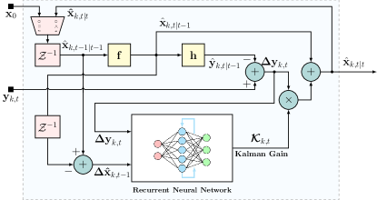
(a) $k^{th}$ forward pass.

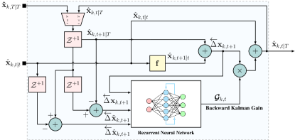
(b) $k^{th}$ backward pass.

Figure 1: rn high level architecture block diagram.

III-B Microarchitecture

rn includes $2K$ rnn, as each $k$th pass utilizes one rnn to compute the forward kg and another rnn to compute the backward kg. In this subsection, we focus on a single pass of index $k$ and formulate the microarchitecture of its forward and backward rnn, as well as which features the rnn use to compute the kg.

Forward Gain: The forward pass is built on kn, where architecture 2 of [39] is particularly utilized to compute the forward kg, i.e., $\mathbfcal{K}_{k,t}$, using separate gru (gru) cells for each of the tracked cov. The division of the architecture into separate gru cells and fc (fc) layers and their interconnection is illustrated in Fig. 2. As shown in the figure, the network composes three gru layers, connected in a cascade with dedicated input and output fc layers. This architecture, which is composed of a non-standard interconnection between gru and fc layers, is directly tailored towards the formulation of the ss model and the operation of the mb kf, as detailed in [39].

The input features are designed to capture differences in the state and the observation model, as these differences are mostly affected by unknown noise statistics. As in [39], the following features are used to compute $\mathbfcal{K}_{k,t}$ (see Fig. 2):

1. Observation difference $\Delta\tilde{\mathbf{y}}_{k,t}={\mathbf{y}_{k,t}-\mathbf{y}_{k,t-1}}$.

2. Innovation difference $\Delta\mathbf{y}_{k,t}=\mathbf{y}_{k,t}-\hat{\mathbf{y}}_{k,t\left|t-1\right.}$.

3. Forward evolution difference $\Delta\tilde{\mathbf{x}}_{k,t}={\hat{\mathbf{x}}_{k,t\left|t\right.}\!-\!\hat{\mathbf{x}}_{k,{t\!-1}\left|t\!-1\right.}}$.

4. Forward update difference $\Delta\hat{\mathbf{x}}_{k,t}={\hat{\mathbf{x}}_{k,t\left|t\right.}-\hat{\mathbf{x}}_{k,{t}\left|t-1\right.}}$.

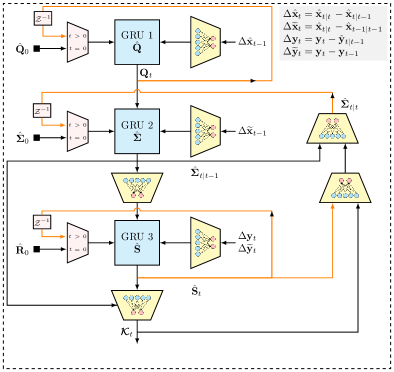
Figure 2: Forward gain rnn block diagram. The input features are used to update three gru with dedicated fc layers, and the overall interconnection between the blocks is based on the flow of the Forward kg $\mathbfcal{K}_{t}$ computation in the mb kf.

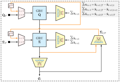
Figure 3: Backward gain rnn block diagram. The input features are used to update two gru with dedicated fc layers, and the overall interconnection between the blocks is based on the flow of the Backward kg $\mathbfcal{G}_{t}$ computation in the ks.

Backward Gain: To compute $\mathbfcal{G}_{k,t}$ in a learned manner, we again design an architecture based on how the ks computes the backward gain. To that aim, we again use separate gru cells for each of the tracked cov, as illustrated in Fig. 3. The first gru layer tracks the unknown state noise covariance $\mathbf{Q}$, thus tracking $m^{2}$ variables. Similarly, the second gru tracks the predicted moment $\hat{\mathbf{\Sigma}}_{t|T}$ (9b) and $\hat{\mathbf{S}}_{t}$ (6b), thus having $m^{2}$ hidden state variables. The gru are interconnected such that the learned $\mathbf{Q}$ is used to compute $\hat{\mathbf{\Sigma}}_{t|T}$, while fc layers are utilized for input and output shaping.

We utilize the following features, which are related to the unknown underlying statistics:

1. Update difference $\overleftarrow{\Delta}\mathbf{x}_{k,t+1}=\hat{\mathbf{x}}_{k,t+1\left|T\right.}-\hat{\mathbf{x}}_{k,t+1\left|t\right.}$.

2. Backward forward difference $\overleftarrow{\Delta}\hat{\mathbf{x}}_{k,t\!+1}\!=\!\\ \hat{\mathbf{x}}_{k,t\!+\!1\left|T\right.}\!-\!\hat{\mathbf{x}}_{k,t\!+\!1\left|t\!+\!1\right.}$.

3. Evolution difference $\overleftarrow{\Delta}\tilde{\mathbf{x}}_{k,t+1}=\hat{\mathbf{x}}_{k,t+2\left|T\right.}-\hat{\mathbf{x}}_{k,t+1\left|T\right.}$.

The first two features capture the uncertainty in the state estimate, where the differences remove predictable components such that they are mostly affected by the unknown noise statistics. The third feature is related to the evolution of the predicted state and thus reflects on its statistics that are tracked by the ks. The features are utilized by the proposed architecture, as illustrated in Fig. 3.

III-C Training Algorithm

Loss Function: We train rn in a supervised manner. To formulate the loss function used for training, let $\mathbf{\Theta}_{k}$ denote the trainable parameters of the rnn of the $k$th pass. The loss measure used to tune these parameters is the regularized $\ell_{2}$ loss; for a labeled pair $(\mathbf{Y}_{k}{(i)},\mathbf{X}^{(i)})$ of length $T_{i}$, this loss is given by

$$\mathcal{L}_{k}^{(i)}\left(\mathbf{\Theta}_{k}\right)= \frac{1}{T_{i}}\cdot\sum_{t=1}^{T_{i}}\left\|\hat{\mathbf{x}}_{k,t\left|T\right.}\left(\mathbf{Y}_{k}^{(i)},\mathbf{\Theta}_{k}\right)-\mathbf{x}^{\left(i\right)}_{t}\right\|^{2}$$

$$+\gamma_{k}\cdot\left\|\mathbf{\Theta}_{k}\right\|^{2}.$$ (17)

In (17), $\hat{\mathbf{x}}_{k,t\left|T\right.}\left(\mathbf{Y}_{k},\mathbf{\Theta}_{k}\right)$ denotes the $t$th output of the $k$th pass with input $\mathbf{Y}_{k}$ and rnn parameters $\mathbf{\Theta}_{k}$. While the loss in (17) refers to a single trajectory $i$, we use it to optimize rn using variants of mini-batch stochastic gradient descent. Here for every batch indexed by $j$, we choose $B<N$ trajectories indexed by $i_{1}^{j},\ldots,i_{B}^{j}$, and compute the mini-batch loss of the $k$th pass as

$$\bar{\mathcal{L}}_{k,j}\left(\mathbf{\Theta}_{k}\right)=\frac{1}{B}\sum_{b=1}^{B}\mathcal{L}_{k}^{(i_{b}^{j})}\left(\mathbf{\Theta}_{k}\right).$$ (18)

Gradient Computation: rn uses the rnn for computing the kg rather than for directly producing the estimate $\hat{\mathbf{x}}_{k,t|T}$. The loss function (17) enables the evaluation of the overall system without having to externally provide ground truth values of the kg for training purposes. Training rn in an e2e manner thus builds upon the ability to backpropagate the loss to the computation of the kg. One can obtain the loss gradient with respect to the kg from the output of rn since by combing (7a) and (9a) we get that

$$\hat{\mathbf{x}}_{k,t\left|T\right.}=\hat{\mathbf{x}}_{k,t\left|t-1\right.}+\mathbfcal{K}_{k,t}\cdot\Delta\mathbf{y}_{k,t}+\mathbfcal{G}_{k,t}\cdot\overleftarrow{\Delta}\mathbf{x}_{k,t+1}.$$ (19)

Consequently, the gradients of the $\ell_{2}$ loss terms with respect to the kg obey

$$\frac{\partial}{\partial\mathbfcal{K}_{k,t}}\left\|\hat{\mathbf{x}}_{k,t\left|T\right.}-\mathbf{x}_{t}\right\|^{2} \propto\left(\mathbf{x}_{k,t\left|T\right.}-\mathbf{x}_{t}\right)\cdot\Delta\mathbf{y}_{k,t}^{\top}$$ (20a)

$$\frac{\partial}{\partial\mathbfcal{G}_{k,t}}\left\|\hat{\mathbf{x}}_{k,t\left|T\right.}-\mathbf{x}_{t}\right\|^{2} \propto\left(\mathbf{x}_{k,t\left|T\right.}-\mathbf{x}_{t}\right)\cdot\overleftarrow{\Delta}\mathbf{x}_{k,t+1}^{\top},$$ (20b)

which in turn allows to compute the gradient of the $\ell_{2}$ loss with respect to $\mathbf{\Theta}_{k}$ via the chain rule. The gradient computation indicates that one can learn the computation of the kg by training rn e2e.

End-to-End Training: The differentiable loss function in (17) allows e2e training of a single forward-backward pass of index $k$. To train the overall unfolded rn, we consider the following loss measures:

Joint learning, where the rnn of all the passes are simultaneously using the labeled dataset $\mathcal{D}$. Here, we stack the trainable parameters as $\mathbf{\Theta}=\{\mathbf{\Theta}_{k}\}$, and set the loss function for the $i$th trajectory to

$$\mathcal{L}^{(i)}\left(\mathbf{\Theta}\right)= \sum_{k=1}^{K}\alpha_{k}\cdot\left(\frac{1}{T_{i}}\cdot\sum_{t=1}^{T_{i}}\left\|\hat{\mathbf{x}}_{k,t\left|T\right.}\left(\mathbf{Y}_{1}^{(i)},\mathbf{\Theta}\right)-\mathbf{x}^{\left(i\right)}_{t}\right\|^{2}\right)$$

$$+\gamma\cdot\left\|\mathbf{\Theta}\right\|^{2}.$$ (21)

where $\hat{\mathbf{x}}_{k,t\left|T\right.}\left(\mathbf{Y}_{1},\mathbf{\Theta}\right)$ is the $t$th output of the $k$th forward-backward pass when the input to rn is $\mathbf{Y}_{1}$ and its parameters are $\mathbf{\Theta}$. The coefficients $\{\alpha_{k}\}_{k=1}^{K}$ in (21) balance the contribution of each pass to the loss – setting $\alpha_{k}=0$ for $k<K$ evaluates rn based solely on its output, while setting $\alpha_{k}\neq 0$ for $k<K$ encourages also the intermediate passes to provide accurate estimates. The ability to evaluate rn during training, not just based on its output but also on its intermediate pass (i.e., with$\alpha_{k}\neq 0$ for $k<K$), is a direct outcome of its interpretable deep unfolded design. In conventional black-box dnn, one typically cannot associate its internal features with an operational meaning and thus trains it solely based on its output. In contrast, our unfolded architecture ensures that internal modules produce a gradually refined estimate. A candidate setting is $\alpha_{k}=\log(1+k)$, see, e.g., [54, 55].

Sequential learning repeats the training procedure $K$ times, training each pass of index $k$ after its preceding passes have been trained using the same dataset. Here, the dataset $\mathcal{D}$ is first used to train only $\mathbf{\Theta}_{1}$ using (17) with $k=1$; then, $\mathbf{\Theta}_{1}$ is frozen and $\mathbf{\Theta}_{2}$ is trained using (17) with $k=2$ and $\mathbf{Y}_{2}^{(i)}=\hat{X}_{1}^{(i)}$, and the procedure repeats until $\mathbf{\Theta}_{K}$ is trained. This form of training, proposed in [56], exploits the modular structure of the unfolded architecture and tends to be data efficient and simpler to train compared with joint learning, and is also the form of training used in our empirical study presented in Section IV.

III-D Discussion

rn is designed to operate in a hybrid dd/mb manner, combining dl with the classical ks. It is designed by converting the eks into a trainable architecture as a form of discriminative machine learning [48], that directly learns the smoothing task from data while bypassing the need to carry out system identification [57]. By identifying the specific noise-model-dependent computations of the ks and replacing them with a dedicated rnn integrated in the mb flow, rn benefits from the individual strengths of both dd and mb approaches. We particularly note several core differences between rn and its mb counterpart. First, rn is suitable for settings where full knowledge on an underlying ss model describing the dynamics is not available. Furthermore Unlike the eks, rn does not attempt to linearize the ss model, and does not impose a statistical model on the noise signals, while avoiding the need to compute a Jacobian and invert a matrix at each iteration. This notably facilitates operation in high-dimensional nl settings [44]. In addition, rn filters in a nl manner, as, e.g., its forward kg matrix depends on the input $\mathbf{y}_{t}$. Moreover, rn supports multiple learned forward-backward passes. While the number of passes is a hyperparameter that should be set based on system considerations and empirical evaluations, our numerical studies reported in Section IV show that using $K=2$ passes improves accuracy in nl settings where the single pass eks is not optimal. Due to these differences, rn is more robust to model mismatch and can infer more efficiently compared with the ks, as shown in Section IV.

Compared to purely dd state estimation, rn benefits from its model awareness, as it supports systematic inclusion of the available state evolution and observation functions, and does not have to learn its complete operation from data. As empirically observed in Section IV, rn achieves improved mse compared to utilizing rnn for e2e state estimation, and also approaches the mmse performance achieved by the ks in linear Gaussian ss models.

Furthermore, the operation of rn follows the flow of ks rather than being utilized as a bb. This implies that the intermediate features exchanged between its modules have a specific operation meaning, providing interpretability that is often scarce in e2e, dl systems. For instance, the fact that rn learns to compute the kg indicates the possibility of providing not only estimates of the state $\mathbf{x}_{t}$, but also a measure of confidence in this estimate, as the kg can be related to the covariance of the estimate, as initially explored for kn in [45].

While rn is inspired by kn, and shares its architecture for the forward pass, the algorithms are fundamentally different. kn is a filtering method, designed to operate in an adaptive sample-by-sample manner. rn is a smoothing algorithm, which jointly processes a complete observed measurement sequence. The most notable difference is in the addition of a backward pass for rn (which is the main extension of the ks over the kf). However, rn also introduces joint learning along with the forward kg; the ability to unfold the operation into multiple iterative forward-backward passes to facilitate coping with complex nl dynamics; and a dedicated learning procedure, as detailed in Subsection III-C.

The fact that rn preserves the ks flow also indicates potential avenues for future research arising from its combination with established model-based extensions to the mb ks. One such avenue of future research involves the incorporation of adaptive priors [58, 59] or optimization-based extensions of the eks [13, 10, 11, 9, 12] for tackling non-Gaussian distributions and outliers, while possibly leveraging emerging techniques for combining iterative methods with deep learning techniques [41, 60]. An alternative research avenue involves extending rn to constrained smoothing [61]. This can potentially be achieved by leveraging the fact that it preserves the operation of the eks and thus supports complying with some forms of state constraints by principled incorporation of differentiable projection operators [62]. These extensions of rn are left for future investigation.

While we train rn in a supervised manner using labeled data, the fact that it preserves the operation of the ks indicates the possibility of training it in an unsupervised manner using a loss function measuring consistency between its estimates and observations, e.g., $\left\|\mathbf{h}\left(\hat{\mathbf{x}}_{t\left|T\right.}\right)-\mathbf{y}_{t}\right\|^{2}$. One can thus envision rn being trained offline in a supervised manner, while tracking variations in the underlying ss model at run-time using online self-supervision. This approach was initially explored for kn in [46], and we leave its extension to future work. The ability to train in an unsupervised manner opens the door to use the backbone of rn in more ss related tasks other than smoothing, e.g., signal de-noising [63], imputation, and prediction. Nonetheless, we leave the exploration of these extensions of rn for future work.

IV Experiments and Results

In this section, we present an extensive empirical study of rn, evaluating its performance in multiple setups and comparing it with both mb and dd benchmark algorithms. We consider both linear Gaussian ss models, where we identify the ability of rn to coincide with the ks (which is mse optimal in such settings), as well as challenging nl models.

IV-A Experimental Setup

Smoothers: Our empirical study compares rn with mb and dd counterparts. We use the ks (rts smoother) as the mb benchmark for linear models. For nl models, we use the eks and the ps [64], where the latter is based on the forward-filter backward simulator of [65] with $100$ particles and $10$ backward trajectories. The benchmark algorithms were optimized for performance by manually tuning the covariance matrices. This tuning is often essential to avoid divergence under model uncertainty as well as under dominant nonlinearities.

Our main dd benchmark is the hybrid graph neural network-aided belief propagation smoother of [38] (referred to as hybrid), which incorporates knowledge of the ss model. We also compare with a bb architecture using a vanilla (vanilla), which is comprised of bi-directional gru with input and output fc layers designed to have a similar number of trainable parameters as rn. Both dnn-aided benchmarks are empirically optimized and cross-validated to achieve their best training performance.

We use the term full information to describe cases where $\mathbf{f}\left(\cdot\right)$ and $\mathbf{h}\left(\cdot\right)$ are accurately known. The term partial information refers to the case where rn and benchmark algorithms operate with some level of model mismatch in their available knowledge of the ss model parameters. rn and the dd vanilla operate without access to the noise covariance matrices (i.e., $\mathbf{Q}$ and $\mathbf{R}$), while their mb counterparts operate with an accurate knowledge of the noise covariance matrices from which the data was generated.

Evaluation: The metric used to evaluate the performance is the empirical mean and standard deviation of squared error, denoted,$\hat{\mu}$ and $\hat{\sigma}$, respectively. Unless stated otherwise, we evaluate using a $N_{\mathrm{test}}=200$ test trajectories.

Throughout the empirical study and unless stated otherwise, in the experiments involving synthetic data, the ss model is generated using diagonal noise covariance matrices; i.e.,

$$\mathbf{Q}=\mathrm{q}^{2}\cdot\mathbf{I},\quad\mathbf{R}=\mathrm{r}^{2}\cdot\mathbf{I},\quad\nu\triangleq\frac{\mathrm{q}^{2}}{\mathrm{r}^{2}}.$$ (22)

By (22), setting $\nu$ to be $0$ dB implies that both the state noise and the observation noise have the same variance.

TABLE I: Linear ss model - Full Information - mse $\left[\textrm{dB}\right]$

(a) $\nu=0\left[\textrm{dB}\right]$

$\mathrm{r}^{2}\left[\textrm{dB}\right]$	$10$	$0$	$-10$	$-20$	$-30$
Noise	10.023	0.054	-10.003	-19.947	-29.962
	$\pm$ 0.424	$\pm$ 0.448	$\pm$ 0.427	$\pm$ 0.411	$\pm$ 0.430
kf	8.085	-1.827	-11.880	-21.903	-31.886
	$\pm$ 0.502	$\pm$ 0.525	$\pm$ 0.464	$\pm$ 0.419	$\pm$ 0.514
ks	6.215	-3.710	-13.776	-23.751	-33.749
	$\pm$ 0.487	$\pm$ 0.535	$\pm$ 0.466	$\pm$ 0.519	$\pm$ 0.508
rn	6.225	-3.695	-13.738	-23.732	-33.698
	$\pm$ 0.487	$\pm$ 0.537	$\pm$ 0.463	$\pm$ 0.512	$\pm$ 0.506

(b) $\nu=-10\left[\textrm{dB}\right]$

$\mathrm{r}^{2}\left[\textrm{dB}\right]$	$10$	$0$	$-10$	$-20$	$-30$
Noise	10.004	0.000	-10.029	-19.982	-29.969
	$\pm$ 0.419	$\pm$ 0.392	$\pm$ 0.431	$\pm$ 0.404	$\pm$ 0.435
kf	5.299	-4.703	-14.756	-24.680	-34.731
	$\pm$ 0.710	$\pm$ 0.663	$\pm$ 0.675	$\pm$ 0.596	$\pm$ 0.696
ks	1.834	-8.220	-18.179	-28.098	-38.236
	$\pm$ 0.794	$\pm$ 0.721	$\pm$ 0.778	$\pm$ 0.726	$\pm$ 0.837
rn	1.881	-8.169	-18.092	-27.875	-38.183
	$\pm$ 0.796	$\pm$ 0.720	$\pm$ 0.797	$\pm$ 0.746	$\pm$ 0.836

(c) $\nu=-20\left[\textrm{dB}\right]$

$\mathrm{r}^{2}\left[\textrm{dB}\right]$	$10$	$0$	$-10$	$-20$	$-30$
Noise	10.012	-0.008	-10.004	-19.977	-30.003
	$\pm$ 0.398	$\pm$ 0.434	$\pm$ 0.448	$\pm$ 0.416	$\pm$ 0.429
kf	2.756	-7.254	-17.339	-27.194	-37.324
	$\pm$ 1.086	$\pm$ 1.012	$\pm$ 0.967	$\pm$ 1.011	$\pm$ 0.963
ks	-1.790	-11.847	-21.738	-31.620	-41.831
	$\pm$ 1.242	$\pm$ 1.190	$\pm$ 1.281	$\pm$ 1.107	$\pm$ 1.289
rn	-1.640	-11.712	-21.543	-31.817	-41.505
	$\pm$ 1.199	$\pm$ 1.173	$\pm$ 1.279	$\pm$ 1.152	$\pm$ 1.229

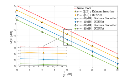
Figure 4: Linear SS model - full information.

IV-B Linear State Space Models with Full Information

We first focus on comparing rn with the ks for synthetically generated linear Gaussian dynamics with full information. Since the ks is mse optimal here, we show that the performance of both algorithms coincides, demonstrating that rn with $K=1$ can learn to be optimal. Then, we show that the learning capabilities of rn are scalable, namely, that they hold for different ss dimensions, and transferable, i.e., that they can be trained and evaluated with different trajectory lengths and initial conditions. We conclude this study by demonstrating the ability of rn to learn to smooth in the presence of non-Gaussian ss models.

Approaching Optimality: We consider a $2\times 2$ ss model (1)-(2), where $\mathbf{F}$ takes a canonical form and $\mathbf{H}$ is set to be the identity matrix, namely,

$$\mathbf{F}=\begin{pmatrix}1&1\\ 0&1\end{pmatrix},\quad\mathbf{H}=\mathbf{I}.$$ (23)

We use multiple noise levels, in $\left[\textrm{dB}\right]$ scale, of $\mathrm{r^{2}}\in\left\{10,0,-10,-20,-30\right\}$, and $\nu\in\left\{-20,-10,0\right\}$. The results provided in Table I(c), and in Fig. 4, show that rn converges to the mmse estimate produced by the ks in the first two moments. This indicates that rn successfully learns to implement the ks when it is mmse optimal.

Scaling up Model Size: Next, we provide empirical evidence that rn is a scalable smoothing architecture, capable of handling ss models beyond just those with small dimensions. In this experiment $\mathbf{F}$ and $\mathbf{H}$ in their canonical form were considered, $\mathrm{q^{2}}=-20\left[\textrm{dB}\right]$, $\mathrm{r^{2}}=0\left[\textrm{dB}\right]$, and $T=20$. It is clearly observed in Table II(a) that rn retains its optimality also for high dimensional models, outperforming its dd benchmarks: vanilla is far from optimal, and the performance of hybrid degrades when the model dimensions increase.

Trajectory Length: To show generalization in $T$, the ss model in (23) is again considered, where $\mathrm{q^{2}}=-20\left[\textrm{dB}\right]$, and $\mathrm{r^{2}}=0\left[\textrm{dB}\right]$. Here, we first train rn and its dd benchmarks on one trajectory length and then test it on a longer one. The results reported in Table II(b) show that while rn retains optimally for various trajectory lengths, vanilla completely diverges. We can also see the superiority of rn over hybrid demonstrating slightly degraded performance.

Initial Conditions: The operation of all smoothing algorithms depends on their initial state. We next train the dd benchmarks on trajectories with a different initial state compared to that used in the test for the ss model in (23) with $\mathrm{q^{2}}=-20\left[\textrm{dB}\right]$, $\mathrm{r^{2}}=0\left[\textrm{dB}\right]$, and $T=100$. The results provided in Table II(c) demonstrates that while vanilla completely diverges, and hybrid is with slightly degraded performance when trained and then tested on different initial conditions, rn still retains its optimally, which again demonstrates that it learns the smoothing task, rather than to overfit to trajectories presented during training.

Non-Gaussian Noise: The fact that rn augments the computation of the forward and backward gains with dedicated rnn enables it to track in non-Gaussian dynamics, where the mb ks is no longer optimal. To demonstrate this, we consider a linear ss model as in (23) where the noise signals are drawn from an i.i.d. exponential distributions with covariance matrices given in (22). For this setting, we compare rn with the mb ks and kf, as well as with the dd hybrid, for $\nu=-20\left[\textrm{dB}\right]$. The resulting mse versus $1/\mathrm{r}^{2}$ are reported in Fig. 5. There, it is clearly observed that rn outperforms not only the mb ks with a notable gap, but also the dd hybrid. These results indicate the ability of the hybrid architecture of rn to successfully cope with non-Gaussian dynamics.

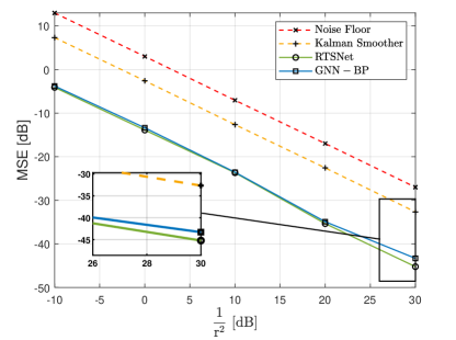
Figure 5: Linear non-Gaussian SS model - full information.

TABLE II: Linear ss model - Learning Capabilities

(a) Scaling ss Model Dimensions

Dimensions	$2\times 2$	$5\times 5$	$10\times 10$	$20\times 20$
kf	-7.791	-10.931	-11.062	-11.540
	$\pm$ 2.204	$\pm$ 1.411	$\pm$ 0.951	$\pm$ 0.771
ks	-11.732	-12.350	-12.436	-12.762
	$\pm$ 2.489	$\pm$ 1.561	$\pm$ 1.058	$\pm$ 0.808
vanilla	3.289	4.261	5.581	3.742
	$\pm$ 4.495	$\pm$ 4.724	$\pm$ 4.553	$\pm$ 4.416
hybrid	-10.016	-9.028	-8.674	-8.557
	$\pm$ 2.331	$\pm$ 1.312	$\pm$ 0.803	$\pm$ 0.603
rn	-11.208	-11.9725	-12.0231	-12.2755
	$\pm$ 2.438	$\pm$ 1.597	$\pm$ 1.055	$\pm$ 0.828

(b) Scalability for Trajectory Length

$T_{\textrm{training}},T_{\textrm{testing}}$	$20,20$	$100,100$	$100,1000$	$100,\mathcal{U}\left[100,1000\right]$
Noise	0.025	-0.008	0.011	0.015
	$\pm$0.919	$\pm$ 0.434	$\pm$ 0.132	$\pm$ 0.227
kf	-7.791	-7.254	-7.162	-7.241
	$\pm$ 2.204	$\pm$ 1.012	$\pm$ 0.335	$\pm$ 0.543
ks	-11.732	-11.847	-11.810	-11.853
	$\pm$ 2.489	$\pm$ 1.190	$\pm$ 0.450	$\pm$ 0.687
vanilla	3.289	22.277	54.955	48.390
	$\pm$ 4.495	$\pm$ 5.190	4.419	5.436
hybrid	-10.016	-11.433	-11.662	-11.687
	$\pm$ 2.331	$\pm$ 1.166	$\pm$ 0.448	$\pm$ 1.740
rn	-11.208	-11.753	-11.753	-11.773
	$\pm$ 2.438	$\pm$ 1.182	$\pm$ 0.449	$\pm$ 0.685

(c) Initial Conditions

Training, Testing	Fixed, Fixed	Fixed, Random	Random, Random
Noise	-0.008	NA	-0.019
	$\pm$ 0.434	NA	$\pm$ 0.360
kf	-7.254	NA	-7.426
	$\pm$ 1.012	NA	$\pm$ 0.963
ks	-11.847	NA	-12.025
	$\pm$ 1.190	NA	$\pm$ 1.238
vanilla	22.277	37.281	26.606
	$\pm$ 5.190	$\pm$ 2.003	$\pm$ 3.547
hybrid	-11.433	-10.655	-11.382
	$\pm$ 1.166	$\pm$ 1.219	$\pm$ 1.164
rn	-11.753	-11.757	-11.701
	$\pm$ 1.182	$\pm$ 1.187	$\pm$ 1.214

IV-C Linear SS Models with Partial Information

Next, we demonstrate the merits of using rn in linear settings with partial information where the ks is degraded due to the missing information. We consider mismatches in both the observation model as well as in the state evolution model. In particular, a mismatch in a model, e.g., the observation model, refers to a case in which a wrong setting of $\mathbf{h}(\cdot)$ is used, while the mb smoothers have access to the noise distribution. We also consider the case in which the corresponding model is unknown, e.g., both $\mathbf{h}(\cdot)$ and the noise distribution are unknown for the observation model; In such cases, since unlike hybrid and the mb benchmarks, rn does not require prior knowledge of the noise distribution, we also evaluate it when it uses its data also to estimate the missing design parameter, e.g., $\mathbf{h}(\cdot)$, using ls.

Observation Model Mismatch: We first consider the case where the design observation model is mismatched. We again use the canonical model in (23) with the observation matrix being either unknown, or assumed to be $\mathbf{H}_{0}=\mathbf{I}$, while the observation model is

$$\mathbf{H}_{\alpha^{\circ}}=\mathbf{R}_{x,y}\left(\alpha\right)\cdot\mathbf{H}_{0},\quad\mathbf{R}_{x,y}\left(\alpha\right)=\begin{pmatrix}\cos{\alpha}&-\sin{\alpha}&0\\ \sin{\alpha}&\cos{\alpha}&0\\ 0&0&1\end{pmatrix},$$

with $\mathbf{H}_{0}=\mathbf{I}$. The data is generated with $\alpha^{\circ}=10$. Such scenarios represent a setup where the true observed values are rotated by $\alpha^{\circ}$, e.g., a slight misalignment of the sensors exists.

We compare the performance of rn and the ks when their design observation model is either $\mathbf{H}_{\alpha=10}$ (full information) or $\mathbf{H}_{\alpha=0}$ (mismatch). We also consider the case where the matrix is estimated from the data set via ls, denoting $\hat{\mathbf{H}}_{\alpha=10}$. The empirical results reported in Table III and in Fig. 6 demonstrate that while ks experienced a severe performance degradation, rn is able to compensate for mismatches using the learned kg. When assuming a mismatched model $\mathbf{H}_{0}$, rn converges to within a minor gap from the mmse, which is further reduced when the data is also used to estimate the observation model. The latter indicates that even when the ss model is completely unknown, yet can be postulated as being linear, rn can reliably smooth by using its data to both estimate the state evolution matrix as well as learn to smooth, while bypassing the need to impose a model on the noise.

TABLE III: Linear ss - Observation mismatch: $\nu=-20\left[\textrm{dB}\right]$

$\mathrm{r}^{2}\left[\textrm{dB}\right]$		$10$	$0$	$-10$	$-20$	$-30$
kf	Full	2.702	-7.394	-17.367	-27.293	-37.273
		$\pm$ 0.885	$\pm$ 0.901	$\pm$ 0.957	$\pm$ 0.966	$\pm$ 1.029
ks	Full	-1.875	-11.880	-21.812	-31.961	-41.810
		$\pm$ 1.285	$\pm$ 1.272	$\pm$ 1.149	$\pm$ 1.265	$\pm$ 1.156
vanilla	Opt	33.490	22.120	13.523	4.058	-5.876
		$\pm$ 4.490	$\pm$ 4.808	$\pm$ 5.334	$\pm$ 4.543	$\pm$ 4.421
hybrid	Full	-1.417	-11.397	-21.383	-31.545	-41.395
		$\pm$ 1.244	$\pm$ 1.248	$\pm$ 1.148	$\pm$ 1.252	$\pm$ 1.200
rn	Full	-1.790	-11.847	-21.738	-31.620	-41.831
		$\pm$ 1.242	$\pm$ 1.190	$\pm$ 1.281	$\pm$ 1.107	$\pm$ 1.289
kf	Partial	11.154	0.926	-9.160	-18.428	-28.786
		$\pm$ 3.023	$\pm$ 3.064	$\pm$ 3.651	$\pm$ 3.253	$\pm$ 3.301
ks	Partial	5.502	-4.825	-15.062	-24.198	-34.592
		$\pm$ 2.942	$\pm$ 3.205	$\pm$ 3.440	$\pm$ 3.119	$\pm$ 3.133
hybrid	Partial	-0.989	-11.123	-20.865	-30.080	-38.174
		$\pm$ 1.223	$\pm$ 1.243	$\pm$ 1.587	$\pm$ 1.354	$\pm$ 2.624
rn	Partial	-0.774	-10.852	-21.104	-29.667	-38.066
		$\pm$ 1.243	$\pm$ 1.158	$\pm$ 1.216	$\pm$ 1.215	$\pm$ 1.136
rn	$\hat{\mathbf{H}}$	-1.743	-11.697	-21.721	-31.186	-40.301
		$\pm$ 1.269	$\pm$ 1.241	$\pm$ 1.153	$\pm$ 1.220	$\pm$ 1.169

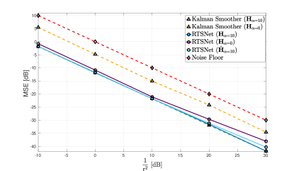
Figure 6: Linear SS model - Observation mismatch.

State Evolution Mismatch: We next consider a similar, but more challenging use case. Here, the design evolution model is either unknown, or assumed to be $\mathbf{F}_{0}=\mathbf{I}$, while the true evolution model is

$$\mathbf{F}_{\alpha^{\circ}}=\mathbf{R}_{x,y}\left(\alpha\right)\cdot\mathbf{F}_{0},\quad\alpha^{\circ}=10.$$ (24)

The empirical results reported in Table IV demonstrate that while ks experienced a severe performance degradation, rn is able to compensate for unknown model information, by pre-estimating the evolution model via ls, and achieve the lb. We can again clearly notice the performance superiority of our rn over its dd counterparts, both for full and unknown information.

TABLE IV: Linear ss - Evolution mismatch: $\nu=-20\left[\textrm{dB}\right]$

$\mathrm{r}^{2}\left[\textrm{dB}\right]$		$10$	$0$	$-10$	$-20$	$-30$
kf	Full	3.450	-6.594	-16.562	-26.601	-36.565
		$\pm$ 1.846	$\pm$ 1.883	$\pm$ 1.876	$\pm$ 1.907	$\pm$ 1.831
ks	Full	-3.843	-13.913	-23.592	-33.861	-43.593
		$\pm$ 2.655	$\pm$ 2.709	$\pm$ 2.751	$\pm$ 2.753	$\pm$ 2.746
vanilla	Opt	40.915	30.714	20.796	12.593	2.411
		$\pm$ 5.033	$\pm$ 5.317	$\pm$ 4.955	$\pm$ 4.281	$\pm$ 4.069
hybrid	Full	-1.975	-11.850	-21.403	-30.579	-41.016
		$\pm$ 2.549	$\pm$ 3.369	$\pm$ 2.564	$\pm$ 2.548	$\pm$ 2.682
rn	Full	-3.351	-13.585	-23.333	-33.126	-43.160
		$\pm$ 2.699	$\pm$ 2.673	$\pm$ 2.671	$\pm$ 2.628	$\pm$ 2.649
kf	Partial	33.961	23.833	13.848	4.199	-6.434
		$\pm$ 3.933	$\pm$ 3.857	$\pm$ 3.683	$\pm$ 3.850	$\pm$ 3.812
ks	Partial	32.963	22.838	12.853	3.201	-7.431
		$\pm$ 3.933	$\pm$ 3.859	$\pm$ 3.685	$\pm$ 3.851	$\pm$ 3.809
hybrid	Partial	12.150	-1.152	-5.042	-10.950	-26.154
		$\pm$ 4.215	$\pm$ 6.240	$\pm$ 4.272	$\pm$ 2.790	$\pm$ 3.968
rn	Partial	10.553	-2.011	-10.689	-21.683	-31.887
		$\pm$ 3.151	$\pm$ 1.945	$\pm$ 1.934	$\pm$ 1.643	$\pm$ 1.244
rn	$\hat{\mathbf{F}}$	-3.433	-12.945	-23.013	-32.932	-41.864
		$\pm$ 2.633	$\pm$ 2.682	$\pm$ 2.798	$\pm$ 2.471	$\pm$ 2.657

IV-D Kinematic Linear Differential Equations

As a concluding experiment in a setting of linear ss models, we consider smoothing in dynamics obtained from a sde (sde) with a model mismatch. The state here represents a moving object obeying the ca (ca) model [49] for one-dimensional kinematics. Here, $\mathbf{x}_{t}=\left(p_{t},v_{t},a_{t}\right)^{\top}\in\mathbb{R}^{3}$, where $p_{t}$, $v_{t}$, and $a_{t}$ are the position, velocity, and acceleration, respectively, at time $t$. We observe noisy position measurements sampled at time intervals $\Delta{t}=10^{-2}$, yielding a linear Gaussian ss model with $\mathbf{H}=\left(1,0,0\right)$ and

$$\mathbf{F}\!=\!\begin{pmatrix}1&\Delta\tau&\frac{1}{2}\Delta\tau^{2}\\ 0&1&\Delta\tau\\ 0&0&1\end{pmatrix};\mathbf{Q}\!=\!\mathrm{q}^{2}\cdot\begin{pmatrix}\frac{1}{20}\Delta\tau^{5}&\frac{1}{8}\Delta\tau^{4}&\frac{1}{6}\Delta\tau^{3}\\ \frac{1}{8}\Delta\tau^{4}&\frac{1}{3}\Delta\tau^{3}&\frac{1}{2}\Delta\tau^{2}\\ \frac{1}{6}\Delta\tau^{3}&\frac{1}{2}\Delta\tau^{2}&\Delta\tau\end{pmatrix}.$$

While for the synthetic linear models considered in the previous subsections we used rn with a single forward-backward pass, here we evaluate it with $K=2$ unfolded pass, comparing it to both the ks and to hybrid when recovering the entire state vector, as well as when recovering only the position (which is often the case in positioning applications). For the latter, we also consider the case where the smoothers assume a more simplified cv (cv) model [49] state evolution for state evolution. The cv model captures in its state vector the position and velocity (without the acceleration), and is a popular model for kinematics due to its simplicity. Yet, for the current setting, it induces an inherent model mismatch. The results are reported in Table V.

For the hybrid smoother of [38], which is dd yet also requires knowledge of the ss model, we optimized $\mathbf{Q}$ via grid search to achieve the best performance, as it was shown to be unstable when substituting the true $\mathbf{Q}$. In Table V, we observe that rn comes within a minor gap of the ks in estimating both the full state as well as only the positions when it is known that the state obeys the ca model; When it is postulated that the state obeys the cv model, rn outperforms all benchmarks.

TABLE V: Linear kinematic ss model

Model	Error	kf	ks	hybrid	rn-2
ca	Full State	-7.631	-8.791	14.351	-8.432
		$\pm$ 2.891	$\pm$ 3.054	$\pm$ 2.011	$\pm$ 2.974
ca	Position	-22.074	-23.221	-11.456	-22.241
		$\pm$ 3.694	$\pm$ 4.081	$\pm$ 2.037	$\pm$ 3.676
cv	Position	-7.657	-14.752	-10.732	-15.900
		$\pm$ 3.145	$\pm$ 3.308	$\pm$ 1.661	$\pm$ 2.542

In the study reported in Table V, the state trajectory was simulated from a kinematic ca model, which is a linear Gaussian state evolution model. We next show that the improved performance of rn is preserved also when tracking states corresponding to real-world vehicular trajectories, that are only approximated by linear Gaussian models. To that aim, we use the city recordings from the KITTI data set [66], where each sample represents the position of a vehicle in three-dimensional space, with 16 training trajectories, 2 validation trajectories, and 6 testing trajectories, all sampled at intervals of $\Delta t=10^{-2}$. The measurements are noisy observations of the position corrupted by Gaussian noise with covariance $\mathbf{R}=\mathbf{I}_{3}$

In Table VI we compare the mse achieved by rn with $K=1$ to that of the mb kf and ks, where all smoothers assume a cv model on the underlying state trajectory. We observe in Table VI that rn outperforms the mb benchmarks, as it learns from data to compensate for the inherent mismatch in modeling the underlying real-world vehicular trajectory as obeying a cv model.

TABLE VI: KITTI kinematic ss model

Model	kf	ks	rn-1
cv	-21.395	-25.158	-26.566
	$\pm$ 0.486	$\pm$ 0.633	$\pm$ 0.422

IV-E Nonlinear Lorenz Attractor

We proceed to evaluate rn in a nl ss model following the la, which is a three-dimensional chaotic solution to the Lorenz system of ordinary differential equations. This synthetically generated chaotic system exemplifies dynamics formulated with sde, that demonstrates the task of smoothing a highly nl trajectory and a rw practical challenge of handling mismatches due to sampling a ct signal into dt [67]. As the dynamics are nl, here we use rn with both $K=1$ and $K=2$ forward-backward passes, denoted rn-1 and rn-2, respectively.

The la models the movement of a particle in 3D space, i.e., $m=3$, which, when sampled at interval $\Delta\tau$, obeys a state evolution model with $\mathbf{f}\left(\mathbf{x}_{t}\right)=\mathbf{F}\left({\mathbf{x}_{t}}\right)\cdot\mathbf{x}_{t}$, where

$$\mathbf{F}\left({\mathbf{x}_{\tau}}\right)=\mathbf{I}+\sum_{j=1}^{J}\frac{\left(\mathbf{A}\left({\mathbf{x}_{\tau}}\right)\cdot\Delta\tau\right)^{j}}{j!},$$ (25)

with $J$ denoting the order of the Taylor series approximation used to obtain the model (where we use $J=5$ when generating the data), and

$$\mathbf{A}\left({\mathbf{x}_{\tau}}\right)=\begin{pmatrix}-10&10&0\\ 28&-1&-\mathrm{x}_{1,\tau}\\ 0&\mathrm{x}_{1,\tau}&-\frac{8}{3}\end{pmatrix}.$$

We first evaluate rn under noisy rotated state observations, with and without observation model mismatch as well as with sampling mismatches, after which we evaluate it with nl observations.

TABLE VII: la - Observation Mismatch:

$\mathrm{r}^{2}\left[\textrm{dB}\right]$		$10$	$0$	$-10$	$-20$	$-30$
Noise		10.017	0.005	-10.011	-19.942	-29.986
		$\pm$ 0.334	$\pm$ 0.376	$\pm$ 0.368	$\pm$ 0.347	$\pm$ 0.354
ekf	Full	-0.299	-10.533	-20.493	-30.348	-40.483
		$\pm$ 1.084	$\pm$ 1.016	$\pm$ 0.969	$\pm$ 1.016	$\pm$ 0.992
eks	Full	-3.892	-13.752	-23.868	-33.743	-43.755
		$\pm$ 0.996	$\pm$ 1.161	$\pm$ 1.025	$\pm$ 1.013	$\pm$ 1.145
hybrid	Full	-2.263	-12.398	-22.413	-31.040	-42.368
		$\pm$ 1.113	$\pm$ 1.182	$\pm$ 1.076	$\pm$ 1.046	$\pm$ 1.256
rn-2	Full	-3.138	-13.330	-23.304	-33.311	-43.235
		$\pm$ 0.983	$\pm$ 1.195	$\pm$ 1.036	$\pm$ 0.999	$\pm$ 1.112
ekf	Partial	-0.258	-9.747	-15.945	-17.549	-17.752
		$\pm$ 1.073	$\pm$ 0.988	$\pm$ 0.769	$\pm$ 0.325	$\pm$ 0.109
eks	Partial	-3.824	-12.932	-18.957	-20.363	-20.563
		$\pm$ 0.976	$\pm$ 1.122	$\pm$ 0.853	$\pm$ 0.366	$\pm$ 0.126
hybrid	Partial	-1.921	-11.959	-18.724	-23.076	-23.351
		$\pm$ 0.962	$\pm$ 1.308	$\pm$ 0.871	$\pm$ 0.743	$\pm$ 0.472
rn-2	Partial	-3.010	-13.290	-22.620	-31.789	-41.874
		$\pm$ 1.067	$\pm$ 1.175	$\pm$ 1.077	$\pm$ 1.207	$\pm$ 1.216
rn-2	$\hat{\mathbf{H}}$	-3.127	-13.315	-23.158	-32.581	-42.928
		$\pm$ 1.057	$\pm$ 1.194	$\pm$ 1.043	$\pm$ 1.119	$\pm$ 1.145

Figure 7: $T=2000$, $\nu=-20\left[\textrm{dB}\right]$, $\mathbf{h}\left(\cdot\right)=\mathbf{I}$.

Rotated State Observations: Here, we consider the dt state evolution with $\Delta{\tau}=0.02$. The observations model $\mathbf{h}\left(\cdot\right)$ is set to a rotation matrix with $\alpha=1^{\circ}$, whereas $T=100$ and $\nu=-20\left[\textrm{dB}\right]$. As in Subsection IV-C, we consider the cases where the smoothers are aware of the rotation (Full information); when the assumed state evolution is the identity matrix instead of the slightly rotated one (Partial information), as well as when it is estimated from the data set via ls ($\hat{\mathbf{H}}$).

The results reported in Table VII and in Fig. 7 demonstrate that although rn does not have access to the true statistics of the noise, for the case of full observation model information, it still achieves the mse lb. It is also observed that a mismatched state observation model obtained from a seemingly minor rotation causes severe performance degradation for the ks, which is sensitive to model uncertainty, while rn is able to learn from data to overcome such mismatches. Finally, empirical observations reveal that rn consistently surpasses the dd benchmark presented in [38]. Furthermore, the utilization of its unfolding mechanism with $K=2$ forward-backward passes leads to a notable enhancement in performance compared to just a single pass.

Sampling Mismatch: Here, we demonstrate a practical case where a physical process evolves in ct, but the smoother only has access to noisy observations in dt, which then results in an inherent mismatch in the ss model. We generate data from an approximate ct noise-less state evolution $\mathbf{F}\left({\mathbf{x}_{\tau}}\right)$, with high resolution time interval ${\Delta\tau=10^{-5}}$. We then sub-sampled the process by a ratio of $\frac{1}{2000}$ and get a decimated process with $\Delta{t}=0.02$. Finally, we generated noisy observations of the true state, by using an identity observation matrix $\mathbf{h}\left(\cdot\right)=\mathbf{I}$ and non-correlated observation noise with $\mathrm{r}^{2}=0\left[\textrm{dB}\right]$. See an example in Fig. 8: gt, and noisy observations, respectively.

The mse values for smoothing sequences with length $T=3000$, reported in Table VIII, demonstrate that rn overcomes the mismatch induced by representing a ct ss model in dt, achieving a substantial processing gain over its mb and dd counterparts due to its learning capabilities. In Fig. 8, we visualize how this gain is translated into clearly improved smoothing of a single trajectory.

TABLE VIII: mse $\left[\textrm{dB}\right]$ - la with sampling mismatch.

Noise	ekf (ekf)	pf	kn	eks	ps	vanilla	hybrid	rn-1	rn-2
-0.024	-6.316	-5.333	-11.106	-10.075	-7.222	-2.342	-16.479	-15.436	-16.803
$\pm$ 0.049	$\pm$ 0.135	$\pm$ 0.136	$\pm$ 0.224	$\pm$ 0.191	$\pm$ 0.202	$\pm$ 0.092	$\pm$ 0.352	$\pm$ 0.329	$\pm$ 0.301

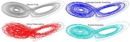
Figure 8: la with sampling mismatch (decimation), $T=3000$.

Noisy Nonlinear Observations: Finally, we consider the case of the dt la, with nl observations, which take the form of a transformation from a cartesian coordinate system to spherical coordinates. In such settings, the observations function is given by

$$\mathbf{h}\left(\left[\mathrm{x},\mathrm{y},\mathrm{z}\right]^{\top}\right)\triangleq\left[\begin{array}[]{c}\sqrt{\mathrm{x}^{2}+\mathrm{y}^{2}+\mathrm{z}^{2}}\\ \tan^{-1}\left(\frac{\mathrm{y}}{\mathrm{x}}\right)\\ \cos^{-1}\left({\frac{\mathrm{z}}{\sqrt{\mathrm{x}^{2}+\mathrm{y}^{2}+\mathrm{z}^{2}}}}\right)\end{array}\right].$$

We further set $T=20$ and $\nu=0\left[\textrm{dB}\right]$.

The mse achieved by rn with $K=2$ forward-backward passes is compared with that of the ks, ps and rn with $K=1$, reported in Table IX and depicted in Fig. 9. It is clearly observed here that in such nl setups, rn outperforms its mb counterparts which operate with full knowledge of the underlying ss model, indicating the ability of its dnn augmentation and unfolded architecture to improve performance in the presence of nonlinearities.

TABLE IX: la with nl observations

$\mathrm{r}^{2}\left[\textrm{dB}\right]$		$10$	$0$	$-10$	$-20$	$-30$
ekf	Full	24.693	12.197	-6.343	-15.574	-26.418
		$\pm$ 4.147	$\pm$ 8.061	$\pm$ 1.961	$\pm$ 3.451	$\pm$ 1.743
eks	Full	24.739	12.045	-7.613	-16.134	-28.211
		$\pm$ 4.313	$\pm$ 8.260	$\pm$ 2.474	$\pm$ 5.157	$\pm$ 1.548
ps	Full	20.490	7.612	-7.093	-17.293	-27.138
		$\pm$ 6.187	$\pm$ 10.071	$\pm$ 1.822	$\pm$ 1.704	$\pm$ 1.743
rn-1	Full	21.094	10.804	-8.074	-17.941	-27.476
		$\pm$ 2.901	$\pm$ 8.999	$\pm$ 1.500	$\pm$ 1.712	$\pm$ 1.553
rn-2	Full	19.849	6.100	-8.122	-17.960	-27.630
		$\pm$ 4.183	$\pm$ 6.614	$\pm$ 1.521	$\pm$ 1.676	$\pm$ 1.558

Figure 9: $T=20$, $\nu=0\left[\textrm{dB}\right]$, $\mathbf{h}\left(\cdot\right)$ nl.

IV-F Nonlinear Van Der Pol Oscillator

The study reported in Subsection IV-E shows the ability of rn to successfully cope with harsh nonlinearities in the ss model. To further demonstrate this property of rn, we next evaluate it in tracking the Van Der Pol Oscillator [68, Sec. 4.1], where the state is a two-dimensional vector governed by the following nl state-evolution model

$$\mathbf{f}\left(\mathbf{x}_{\tau}\right)=\left(\begin{array}[]{c}\mathrm{x}_{1,\tau}+\mathrm{x}_{2,\tau}\cdot\Delta\tau\\ \mathrm{x}_{2,\tau}+\left(2\left(1-\mathrm{x}_{1,\tau}^{2}\right)\cdot\mathrm{x}_{2,\tau}-\mathrm{x}_{1,\tau}\right)\Delta\tau\end{array}\right),$$ (26)

with $\Delta\tau=0.1$ Tracking is done based on noisy observations of the first state element, i.e., $\mathbf{H}=(1,0)$, with $\mathbf{Q}=0.01\cdot\mathbf{I}_{2}$ and $\mathbf{R}=1$. The initial state is fixed to $\mathbf{x}_{0}=(0,-5)^{\top}$, and the trajectory length is $T=40$.

In addition to comparing rn to the mb ekf and eks, here we also compare it to optimization-based smoothers that are derived from the map formulation, and particularly the mb Gauss-Newton method of [9, Sec. 3]. This optimization-based smoother is typically capable of tracking in nl ss models, while coinciding with the mse optimal eks for linear Gaussian cases. The resulting mse values are reported in Table X. There, it is observed that the nl state evolution model in (26) limits the performance of the ekf and the eks, which are outperformed by the Gauss-Newton method of [9]. Still, rn is shown in Table X to outperform all these mb smoothers, which operate with full knowledge of the underlying ss model and the noise distribution.

TABLE X: Van der Pol oscillator

ekf	eks	Gauss-Newton	rn-1
12.711	3.164	-4.94	-7.689
$\pm$ 5.951	$\pm$ 4.135	$\pm$ 2.45	$\pm$ 3.102

IV-G Complexity Analysis

So far, we have demonstrated that rn delivers superior mse performance, surpassing both its dd and mb counterparts, especially when they operate with partial information or under nl dynamics. We conclude our empirical study by highlighting that the advantages of rn don’t come with added computational complexity during inference, dependency on large datasets, or an increase in dnn size

In Table XI, we detail the average inference time for all filters (without parallelism) using the la se task as a benchmark. The stopwatch timings, captured on Google Colab equipped with a CPU: Intel(R) Xeon(R) CPU @ 2.20GHz and GPU: Tesla P100-PCIE-16GB, reveal that rn is highly competitive when compared with classical methods and even outperforms hybrid. This superiority is primarily attributed to its efficient nn computations. Furthermore, unlike the mb filters, rn bypasses the need for linearization and matrix inversions at each time step.

Subsequently, we delve into the volume of training trajectories required to effectively train rn. Focusing again on the la setup, we measure the average mse against varying data sizes. Specifically, each dd smoothing algorithm is trained with a varying number of trajectories (denoted as $N$) spanning a length of $T=3000$ pairs with an observation noise of $\mathrm{r}^{2}=0\left[\textrm{dB}\right]$. As depicted in Fig. 10, which showcases test mse versus $10\log_{10}\left(N\right)$, rn is successfully trained even with a single trajectory. Notably, its performance is approached by dd hybrid only when the number of trajectories exceeds $50$.

Figure 10: mse versus $10\log_{10}(N)$, nl.

In conclusion, a side-by-side comparison of dnn size, represented by the number of trainable parameters, between rn and hybrid for select use cases reveals some insightful findings. Table Table XII lists the number of parameters, illustrating the compactness of rn, thereby implying that it is easier to train. Significantly, rn consistently outperforms the dd hybrid benchmark of [38] across tested scenarios. This is achieved with a simpler architecture that has fewer trainable parameters. This stands out especially considering that the design of [38] also emphasizes compactness and efficiency. Ultimately, The reduced parameterization of rn leads to faster training and inference.

TABLE XI: Inference Time $\left[\sec\right]$ - la.

Use Case	Trajectory Length	kf	pf	kn	ks	ps	hybrid	rn-1	rn-2
Nonlinear Observations	$T=20$	0.0501	NA	NA	0.0946	5.0175	NA	0.0605	0.1178
Linear Observations	$T=100$	0.2194	NA	NA	0.4344	24.4158	1.2513	0.2950	NA
Decimation $\left(K=2\right)$	$T=3000$	4.3583	45.4791	4.9226	6.5164	452.8513	25.4527	7.3587	14.6174
Decimation $\left(K=5\right)$	$T=3000$	6.2641	71.6549	NA	10.3243	723.9320	NA	NA	NA

TABLE XII: Network Size - Number of Trainable Parameters

Use Case	Linear - $2\times 2$	Linear - $5\times 5$	Lorentz - Decimation
rn	$7,370$	$28,285$	$33,270~{}(\#1)~{},~{}66,540~{}(\#2)$
hybrid	$40,947$	$41,814$	$41,236$

V Conclusion

In this work, we introduced rn, a hybrid fusion of dl with the classic ks. Our design identifies the ss-model-dependent computations of the ks and replaces them with dedicated rnn. These rnn operate on specific features that encapsulate the information necessary for their operation. Additionally, we unfold the algorithm to enable multiple trainable forward-backward passes. Our empirical studies reveal that rn can perform offline state estimation similarly to the ks, but with the added ability to learn to overcome model mismatches and nonlinearities. Notably, rn employs a relatively compact rnn, which can be trained with a modest-sized ds, leading to reduced complexity.

Guy Revach is a researcher with a proven industry track record as an innovator and system engineer. He received his B.Sc. (cum laude) and M.Sc. degrees in 2008 and 2017, respectively, from the Andrew and Erna Viterbi Department of Electrical & Computer Engineering at the Technion – Israel Institute of Technology in Haifa. He completed his master’s thesis under the supervision of Prof. Nahum Shimkin on planning for cooperative multi-agents. Since 2019, he has been a Ph.D. candidate at the Institute for Signal and Information Processing (ISI) at ETH Zürich, Switzerland, supervised by Prof. Dr. Hans-Andrea Loeliger. His main research focus is on the intersection of machine learning with signal processing, specifically combining sound theoretical principles from classical signal processing with state-of-the-art machine learning algorithms for tracking and detection problems. Before joining ETH Zürich, he worked in the Israeli wireless communication industry for over 10 years, initially as a real-time embedded software engineer and later as a software manager. He was the main innovator behind state-of-the-art, software-defined radio (SDR) for wireless communication, which was game-changing and groundbreaking in terms of size, weight, and power. As a system engineer, he defined major aspects of SDR requirements and architecture, including hardware, software, network, cyber defense, signal processing, data analysis, and control algorithms.

Xiaoyong Ni received a B.S. degree in Communication Engineering in 2020 from the University of Electronic Science and Technology of China (UESTC) in Chengdu, China. He received an M.S. degree from the Department of Electrical Engineering and Information Technology at ETH Zürich. His current research interests include signal processing, machine learning, and wireless communication.

Nir Shlezinger (M’17-SM’23) is an assistant professor in the School of Electrical and Computer Engineering at Ben-Gurion University, Israel. He received his B.Sc., M.Sc., and Ph.D. degrees in 2011, 2013, and 2017, respectively, from Ben-Gurion University, Israel, all in electrical and computer engineering. From 2017 to 2019, he was a postdoctoral researcher at the Technion, and from 2019 to 2020, he was a postdoctoral researcher at the Weizmann Institute of Science, where he was awarded the FGS Prize for outstanding research achievements. His research interests include communications, information theory, signal processing, and machine learning.

Ruud van Sloun is an Associate Professor at the Department of Electrical Engineering at Eindhoven University of Technology in the Netherlands. He received both his M.Sc. and Ph.D. degrees (cum laude) in Electrical Engineering from Eindhoven University of Technology in 2014 and 2018, respectively. From 2019 to 2020, he served as a Visiting Professor with the Department of Mathematics and Computer Science at the Weizmann Institute of Science in Rehovot, Israel. From 2020 to 2023, he was a Kickstart AI Fellow at Philips Research. He has been honored with an ERC Starting Grant, an NWO VIDI Grant, an NWO Rubicon Grant, and a Google Faculty Research Award. His current research interests include closed-loop image formation, deep learning for signal processing and imaging, active signal acquisition, model-based deep learning, compressed sensing, ultrasound imaging, and probabilistic signal and image reconstruction.

Yonina C. Eldar (S’98-M’02-SM’07-F’12) received the B.Sc. degree in Physics in 1995 and the B.Sc. degree in Electrical Engineering in 1996 both from Tel-Aviv University (TAU), Tel-Aviv, Israel, and the Ph.D. degree in Electrical Engineering and Computer Science in 2002 from the Massachusetts Institute of Technology (MIT), Cambridge. She is currently a Professor in the Department of Mathematics and Computer Science, Weizmann Institute of Science, Rehovot, Israel. She was previously a Professor in the Department of Electrical Engineering at the Technion, where she held the Edwards Chair in Engineering. She is also a Visiting Professor at MIT, a Visiting Scientist at the Broad Institute, and an Adjunct Professor at Duke University and was a Visiting Professor at Stanford. She is a member of the Israel Academy of Sciences and Humanities (elected 2017), an IEEE Fellow and a EURASIP Fellow. Her research interests are in the broad areas of statistical signal processing, sampling theory and compressed sensing, learning and optimization methods, and their applications to biology, medical imaging and optics. Dr. Eldar has received many awards for excellence in research and teaching, including the IEEE Signal Processing Society Technical Achievement Award (2013), the IEEE/AESS Fred Nathanson Memorial Radar Award (2014), and the IEEE Kiyo Tomiyasu Award (2016). She was a Horev Fellow of the Leaders in Science and Technology program at the Technion and an Alon Fellow. She received the Michael Bruno Memorial Award from the Rothschild Foundation, the Weizmann Prize for Exact Sciences, the Wolf Foundation Krill Prize for Excellence in Scientific Research, the Henry Taub Prize for Excellence in Research (twice), the Hershel Rich Innovation Award (three times), the Award for Women with Distinguished Contributions, the Andre and Bella Meyer Lectureship, the Career Development Chair at the Technion, the Muriel & David Jacknow Award for Excellence in Teaching, and the Technion’s Award for Excellence in Teaching (two times). She received several best paper awards and best demo awards together with her research students and colleagues including the SIAM outstanding Paper Prize, the UFFC Outstanding Paper Award, the Signal Processing Society Best Paper Award and the IET Circuits, Devices and Systems Premium Award, was selected as one of the 50 most influential women in Israel and in Asia, and is a highly cited researcher. She was a member of the Young Israel Academy of Science and Humanities and the Israel Committee for Higher Education. She is the Editor in Chief of Foundations and Trends in Signal Processing, a member of the IEEE Sensor Array and Multichannel Technical Committee and serves on several other IEEE committees. In the past, she was a Signal Processing Society Distinguished Lecturer, member of the IEEE Signal Processing Theory and Methods and Bio Imaging Signal Processing technical committees, and served as an associate editor for the IEEE Transactions On Signal Processing, the EURASIP Journal of Signal Processing, the SIAM Journal on Matrix Analysis and Applications, and the SIAM Journal on Imaging Sciences. She was Co-Chair and Technical Co-Chair of several international conferences and workshops. She is author of the book ”Sampling Theory: Beyond Bandlimited Systems” and co-author of five other books published by Cambridge University Press.

References

- [1] X. Ni, G. Revach, N. Shlezinger, R. J. G. van Sloun, and Y. C. Eldar, “RTSNet: Deep Learning Aided Kalman Smoothing,” in IEEE International Conference on Acoustics, Speech and Signal Processing (ICASSP), 2022, pp. 5902–5906.
- [2] J. Durbin and S. J. Koopman, Time series analysis by state space methods. Oxford University Press, 2012.
- [3] N. Wiener, Extrapolation, interpolation, and smoothing of stationary time series: With engineering applications. MIT press Cambridge, MA, 1949, vol. 113, no. 21.
- [4] R. E. Kalman, “A new approach to linear filtering and prediction problems,” Journal of Basic Engineering, vol. 82, no. 1, pp. 35–45, 1960.
- [5] H. E. Rauch, F. Tung, and C. T. Striebel, “Maximum likelihood estimates of linear dynamic systems,” AIAA Journal, vol. 3, no. 8, pp. 1445–1450, 1965.
- [6] H.-A. Loeliger, J. Dauwels, J. Hu, S. Korl, L. Ping, and F. R. Kschischang, “The Factor Graph Approach to Model-Based Signal Processing,” Proceedings of the IEEE, vol. 95, no. 6, pp. 1295–1322, 2007.
- [7] F. Wadehn, State space methods with applications in biomedical signal processing. ETH Zurich, 2019, vol. 31.
- [8] J. Humpherys, P. Redd, and J. West, “A fresh look at the Kalman filter,” SIAM review, vol. 54, no. 4, pp. 801–823, 2012.
- [9] A. Y. Aravkin, J. V. Burke, and G. Pillonetto, “Optimization viewpoint on Kalman smoothing with applications to robust and sparse estimation,” Compressed sensing & sparse filtering, pp. 237–280, 2014.
- [10] A. Y. Aravkin, B. M. Bell, J. V. Burke, and G. Pillonetto, “An -Laplace Robust Kalman Smoother,” IEEE Trans. Autom. Control, vol. 56, no. 12, pp. 2898–2911, 2011.
- [11] A. Y. Aravkin, J. V. Burke, and G. Pillonetto, “Sparse/Robust Estimation and Kalman Smoothing with Nonsmooth Log-Concave Densities: Modeling, Computation, and Theory.” Journal of Machine Learning Research, vol. 14, 2013.
- [12] A. Y. Aravkin and J. V. Burke, “Smoothing dynamic systems with state-dependent covariance matrices,” in IEEE Conference on Decision and Control, 2014, pp. 3382–3387.
- [13] A. Aravkin, J. V. Burke, L. Ljung, A. Lozano, and G. Pillonetto, “Generalized Kalman smoothing: Modeling and algorithms,” Automatica, vol. 86, pp. 63–86, 2017.
- [14] Z. Ghahramani and G. E. Hinton, “Parameter Estimation for Linear Dynamical Systems,” University of Totronto, Dept. of Computer Science, Tech. Rep. CRG-TR-96-2, 02 1996.
- [15] J. Dauwels, A. W. Eckford, S. Korl, and H. Loeliger, “Expectation Maximization as Message Passing - Part I: Principles and Gaussian Messages,” CoRR, vol. abs/0910.2832, 2009. [Online]. Available: http://arxiv.org/abs/0910.2832
- [16] K.-V. Yuen and S.-C. Kuok, “Online updating and uncertainty quantification using nonstationary output-only measurement,” Mechanical Systems and Signal Processing, vol. 66, pp. 62–77, 2016.
- [17] H.-Q. Mu, S.-C. Kuok, and K.-V. Yuen, “Stable robust Extended Kalman filter,” Journal of Aerospace Engineering, vol. 30, no. 2, p. B4016010, 2017.
- [18] L. Martino, J. Read, V. Elvira, and F. Louzada, “Cooperative parallel particle filters for online model selection and applications to urban mobility,” Digital Signal Processing, vol. 60, pp. 172–185, 2017.
- [19] L. Xu and R. Niu, “EKFNet: Learning system noise statistics from measurement data,” in IEEE International Conference on Acoustics, Speech and Signal Processing (ICASSP), 2021, pp. 4560–4564.
- [20] S. T. Barratt and S. P. Boyd, “Fitting a Kalman smoother to data,” in IEEE American Control Conference (ACC), 2020, pp. 1526–1531.
- [21] M. Zorzi, “On the robustness of the Bayes and Wiener estimators under model uncertainty,” Automatica, vol. 83, pp. 133–140, 2017.
- [22] A. Longhini, M. Perbellini, S. Gottardi, S. Yi, H. Liu, and M. Zorzi, “Learning the tuned liquid damper dynamics by means of a robust ekf,” in 2021 American Control Conference (ACC), 2021, pp. 60–65.
- [23] I. Goodfellow, Y. Bengio, and A. Courville, Deep Learning. MIT Press Cambridge, MA, 2016, http://www.deeplearningbook.org.
- [24] J. Chung, C. Gulcehre, K. Cho, and Y. Bengio, “Empirical evaluation of gated recurrent neural networks on sequence modeling,” in NIPS 2014 Workshop on Deep Learning, December 2014, 2014.
- [25] A. Vaswani, N. Shazeer, N. Parmar, J. Uszkoreit, L. Jones, A. N. Gomez, L. u. Kaiser, and I. Polosukhin, “Attention is All you Need,” in Advances in Neural Information Processing Systems, I. Guyon, U. V. Luxburg, S. Bengio, H. Wallach, R. Fergus, S. Vishwanathan, and R. Garnett, Eds., vol. 30. Curran Associates, Inc., 2017. [Online]. Available: https://proceedings.neurips.cc/paper_files/paper/2017/file/3f5ee243547dee91fbd053c1c4a845aa-Paper.pdf
- [26] P. Becker, H. Pandya, G. Gebhardt, C. Zhao, C. J. Taylor, and G. Neumann, “Recurrent Kalman networks: Factorized inference in high-dimensional deep feature spaces,” in International Conference on Machine Learning. PMLR, 2019, pp. 544–552.
- [27] M. Zaheer, A. Ahmed, and A. J. Smola, “Latent LSTM allocation: Joint clustering and non-linear dynamic modeling of sequence data,” in International Conference on Machine Learning, 2017, pp. 3967–3976.
- [28] R. G. Krishnan, U. Shalit, and D. A. Sontag, “Deep Kalman filters,” CoRR, vol. abs/1511.05121, 2015.
- [29] E. Archer, I. M. Park, L. Buesing, J. Cunningham, and L. Paninski, “Black box variational inference for state space models,” arXiv preprint arXiv:1511.07367, 11 2015.
- [30] M. Karl, M. Soelch, J. Bayer, and P. van der Smagt, “Deep Variational Bayes Filters: Unsupervised Learning of State Space Models from Raw Data,” in International Conference on Learning Representations, 2017.
- [31] R. Krishnan, U. Shalit, and D. Sontag, “Structured inference networks for nonlinear state space models,” in Proceedings of the AAAI Conference on Artificial Intelligence, vol. 31, no. 1, 2017.
- [32] M. Fraccaro, S. D. Kamronn, U. Paquet, and O. Winther, “A Disentangled Recognition and Nonlinear Dynamics Model for Unsupervised Learning,” in Advances in Neural Information Processing Systems, 2017.
- [33] T. Haarnoja, A. Ajay, S. Levine, and P. Abbeel, “Backprop KF: Learning discriminative deterministic state estimators,” in Advances in Neural Information Processing Systems, 2016, pp. 4376–4384.
- [34] B. Laufer-Goldshtein, R. Talmon, and S. Gannot, “A hybrid approach for speaker tracking based on TDOA and data-driven models,” IEEE/ACM Trans. Audio, Speech, Language Process., vol. 26, no. 4, pp. 725–735, 2018.
- [35] L. Zhou, Z. Luo, T. Shen, J. Zhang, M. Zhen, Y. Yao, T. Fang, and L. Quan, “KFNet: Learning temporal camera relocalization using Kalman Filtering,” in Proceedings of the IEEE/CVF Conference on Computer Vision and Pattern Recognition, 2020, pp. 4919–4928.
- [36] H. Coskun, F. Achilles, R. DiPietro, N. Navab, and F. Tombari, “Long short-term memory Kalman filters: Recurrent neural estimators for pose regularization,” in Proceedings of the IEEE International Conference on Computer Vision, 2017, pp. 5524–5532.
- [37] S. S. Rangapuram, M. W. Seeger, J. Gasthaus, L. Stella, Y. Wang, and T. Januschowski, “Deep state space models for time series forecasting,” in Advances in Neural Information Processing Systems, 2018, pp. 7785–7794.
- [38] V. G. Satorras, Z. Akata, and M. Welling, “Combining generative and discriminative models for hybrid inference,” in Advances in Neural Information Processing Systems, 2019, pp. 13 802–13 812.
- [39] G. Revach, N. Shlezinger, X. Ni, A. L. Escoriza, R. J. G. van Sloun, and Y. C. Eldar, “KalmanNet: Neural Network Aided Kalman Filtering for Partially Known Dynamics,” IEEE Transactions on Signal Processing, vol. 70, pp. 1532–1547, 2022.
- [40] N. Shlezinger, J. Whang, Y. C. Eldar, and A. G. Dimakis, “Model-Based Deep Learning,” Proceedings of the IEEE, vol. 111, no. 5, pp. 465–499, 2023.
- [41] N. Shlezinger, Y. C. Eldar, and S. P. Boyd, “Model-Based Deep Learning: On the Intersection of Deep Learning and Optimization,” IEEE Access, vol. 10, pp. 115 384–115 398, 2022.
- [42] N. Shlezinger and Y. C. Eldar, “Model-Based Deep Learning,” Foundations and Trends® in Signal Processing, vol. 17, no. 4, pp. 291–416, 2023. [Online]. Available: http://dx.doi.org/10.1561/2000000113
- [43] A. L. Escoriza, G. Revach, N. Shlezinger, and R. J. G. van Sloun, “Data-Driven Kalman-Based Velocity Estimation for Autonomous Racing,” in IEEE International Conference on Autonomous Systems (ICAS), 2021.
- [44] I. Buchnik, D. Steger, G. Revach, R. J. van Sloun, T. Routtenberg, and N. Shlezinger, “Latent-KalmanNet: Learned Kalman Filtering for Tracking from High-Dimensional Signals,” arXiv preprint arXiv:2304.07827, 2023.
- [45] I. Klein, G. Revach, N. Shlezinger, J. E. Mehr, R. J. G. van Sloun, and Y. C. Eldar, “Uncertainty in Data-Driven Kalman Filtering for Partially Known State-Space Models,” in IEEE International Conference on Acoustics, Speech and Signal Processing (ICASSP), 2022, pp. 3194–3198.
- [46] G. Revach, N. Shlezinger, T. Locher, X. Ni, R. J. G. van Sloun, and Y. C. Eldar, “Unsupervised Learned Kalman Filtering,” in European Signal Processing Conference (EUSIPCO), 2022, pp. 1571–1575.
- [47] V. Monga, Y. Li, and Y. C. Eldar, “Algorithm unrolling: Interpretable, efficient deep learning for signal and image processing,” IEEE Signal Process. Mag., vol. 38, no. 2, pp. 18–44, 2021.
- [48] N. Shlezinger and T. Routtenberg, “Discriminative and Generative Learning for the Linear Estimation of Random Signals [Lecture Notes],” IEEE Signal Processing Magazine, vol. 40, no. 6, pp. 75–82, 2023.
- [49] Y. Bar-Shalom, X. R. Li, and T. Kirubarajan, Estimation with applications to tracking and navigation: Theory algorithms and software. John Wiley & Sons, 01 2004.
- [50] S. SÄrkkÄ, “Unscented Rauch–Tung–Striebel Smoother,” IEEE Trans. Autom. Control, vol. 53, no. 3, pp. 845–849, 2008.
- [51] N. J. Gordon, D. J. Salmond, and A. F. Smith, “Novel approach to nonlinear/non-Gaussian Bayesian state estimation,” in IEE proceedings F (radar and signal processing), vol. 140, no. 2. IET, 1993, pp. 107–113.
- [52] G. J. Bierman, Factorization methods for discrete sequential estimation. Courier Corporation, 1977.
- [53] ——, “Fixed interval smoothing with discrete measurements,” International Journal of Control, vol. 18, no. 1, pp. 65–75, 1973.
- [54] N. Samuel, T. Diskin, and A. Wiesel, “Learning to detect,” IEEE Trans. Signal Process., vol. 67, no. 10, pp. 2554–2564, 2019.
- [55] O. Lavi and N. Shlezinger, “Learn to rapidly and robustly optimize hybrid precoding,” IEEE Trans. Commun., 2023, early access.
- [56] N. Shlezinger, R. Fu, and Y. C. Eldar, “DeepSIC: Deep Soft Interference Cancellation for Multiuser MIMO Detection,” IEEE Transactions on Wireless Communications, vol. 20, no. 2, pp. 1349–1362, 2021.
- [57] G. Pillonetto, A. Aravkin, D. Gedon, L. Ljung, A. H. Ribeiro, and T. B. Schön, “Deep networks for system identification: a Survey,” arXiv preprint arXiv:2301.12832, 2023.
- [58] H.-A. Loeliger, L. Bruderer, H. Malmberg, F. Wadehn, and N. Zalmai, “On sparsity by NUV-EM, Gaussian message passing, and Kalman smoothing,” in Information Theory and Applications Workshop (ITA). IEEE, 2016.
- [59] F. Wadehn, L. Bruderer, J. Dauwels, V. Sahdeva, H. Yu, and H.-A. Loeliger, “Outlier-insensitive Kalman smoothing and marginal message passing,” in European Signal Processing Conference (EUSIPCO). IEEE, 2016, pp. 1242–1246.
- [60] A. Agrawal, S. Barratt, and S. Boyd, “Learning convex optimization models,” IEEE/CAA J. Autom. Sinica, vol. 8, no. 8, pp. 1355–1364, 2021.
- [61] N. Amor, G. Rasool, and N. C. Bouaynaya, “Constrained state estimation-a review,” arXiv preprint arXiv:1807.03463, 2018.
- [62] B. Liang, T. Mitchell, and J. Sun, “NCVX: A General-Purpose Optimization Solver for Constrained Machine and Deep Learning,” in OPT 2022: Optimization for Machine Learning (NeurIPS 2022 Workshop), 2022. [Online]. Available: https://openreview.net/forum?id=rg7l9Vrt4-8
- [63] T. Locher, G. Revach, N. Shlezinger, R. J. G. van Sloun, and R. Vullings, “Hierarchical Filtering With Online Learned Priors for ECG Denoising,” in ICASSP 2023 - 2023 IEEE International Conference on Acoustics, Speech and Signal Processing (ICASSP), 2023, pp. 1–5.
- [64] S. J. Godsill, A. Doucet, and M. West, “Monte Carlo smoothing for nonlinear time series,” Journal of the american statistical association, vol. 99, no. 465, pp. 156–168, 2004.
- [65] Jerker Nordh, “pyParticleEst - Particle based methods in Python,” 2015. [Online]. Available: https://pyparticleest.readthedocs.io/en/latest/index.html
- [66] A. Geiger, P. Lenz, C. Stiller, and R. Urtasun, “Vision meets robotics: The KITTI dataset,” The International Journal of Robotics Research, vol. 32, no. 11, pp. 1231–1237, 2013.
- [67] W. Gilpin, “Chaos as an interpretable benchmark for forecasting and data-driven modelling,” in Thirty-fifth Conference on Neural Information Processing Systems Datasets and Benchmarks Track (Round 2), 2021.
- [68] R. Kandepu, B. Foss, and L. Imsland, “Applying the unscented Kalman filter for nonlinear state estimation,” Journal of Process Control, vol. 18, no. 7-8, pp. 753–768, 2008.