Deep Long-Tailed Learning: A Survey

Abstract

Deep long-tailed learning, one of the most challenging problems in visual recognition, aims to train well-performing deep models from a large number of images that follow a long-tailed class distribution. In the last decade, deep learning has emerged as a powerful recognition model for learning high-quality image representations and has led to remarkable breakthroughs in generic visual recognition. However, long-tailed class imbalance, a common problem in practical visual recognition tasks, often limits the practicality of deep network based recognition models in real-world applications, since they can be easily biased towards dominant classes and perform poorly on tail classes. To address this problem, a large number of studies have been conducted in recent years, making promising progress in the field of deep long-tailed learning. Considering the rapid evolution of this field, this paper aims to provide a comprehensive survey on recent advances in deep long-tailed learning. To be specific, we group existing deep long-tailed learning studies into three main categories (i.e., class re-balancing, information augmentation and module improvement), and review these methods following this taxonomy in detail. Afterward, we empirically analyze several state-of-the-art methods by evaluating to what extent they address the issue of class imbalance via a newly proposed evaluation metric, i.e., relative accuracy. We conclude the survey by highlighting important applications of deep long-tailed learning and identifying several promising directions for future research.

1 Introduction

Deep learning allows computational models, composed of multiple processing layers, to learn data representations with multiple levels of abstraction [1, 2] and has made incredible progress in computer vision [3, 4, 5, 6, 7, 8]. The key enablers of deep learning are the availability of large-scale datasets, the emergence of GPUs, and the advancement of deep network architectures [9]. Thanks to the strong ability of learning high-quality data representations, deep neural networks have been applied with great success to many visual discriminative tasks, including image classification [6, 10], object detection [11, 7] and semantic segmentation [12, 8].

In real-world applications, training samples typically exhibit a long-tailed class distribution, where a small portion of classes have a massive number of sample points but the others are associated with only a few samples [13, 14, 15, 16]. Such class imbalance of training sample numbers, however, makes the training of deep network based recognition models very challenging. As shown in Fig. 1, the trained model can be easily biased towards head classes with massive training data, leading to poor model performance on tail classes that have limited data [17, 18, 19]. Therefore, the deep models trained by the common practice of empirical risk minimization [20] cannot handle real-world applications with long-tailed class imbalance, e.g., face recognition [21, 22], species classification [23, 24], medical image diagnosis [25], urban scene understanding [26] and unmanned aerial vehicle detection [27].

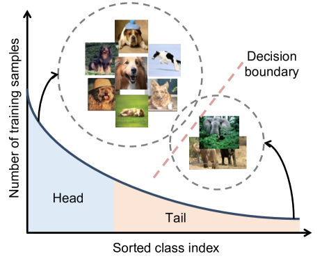
Figure 1: The label distribution of a long-tailed dataset (e.g., the iNaturalist species dataset [23] with more than 8,000 classes). The head-class feature space learned on these sampled is often larger than tail classes, while the decision boundary is usually biased towards dominant classes.

To address long-tailed class imbalance, massive deep long-tailed learning studies have been conducted in recent years [16, 28, 15, 29, 30]. Despite the rapid evolution in this field, there is still no systematic study to review and discuss existing progress. To fill this gap, we aim to provide a comprehensive survey for recent long-tailed learning studies conducted before mid-2021.

As shown in Fig. 2, we group existing methods into three main categories based on their main technical contributions, i.e., class re-balancing, information augmentation and module improvement; these categories can be further classified into nine sub-categories: re-sampling, class-sensitive learning, logit adjustment, transfer learning, data augmentation, representation learning, classifier design, decoupled training and ensemble learning. According to this taxonomy, we provide a comprehensive review of existing methods, and also empirically analyze several state-of-the-art methods by evaluating their abilities of handling class imbalance using a new evaluation metric, namely relative accuracy. We conclude the survey by introducing several real-world application scenarios of deep long-tailed learning and identifying several promising research directions that can be explored by the community in the future.

We summarize the key contributions of this survey as follows.

• To the best of our knowledge, this is the first comprehensive survey of deep long-tailed learning, which will provide a better understanding of long-tailed visual learning with deep neural networks for researchers and the community.

• We provide an in-depth review of advanced long-tailed learning studies, and empirically study state-of-the-art methods by evaluating to what extent they handle long-tailed class imbalance via a new relative accuracy metric.

• We identify four potential directions for method innovation as well as eight new deep long-tailed learning task settings for future research.

The rest of this survey will be organized as follows: Section 2 presents the problem definition and introduces widely-used datasets, metrics and applications. Section 3 provides a comprehensive review of advanced long-tailed learning methods and Section 4 empirically analyzes several state-of-the-art methods based on a new evaluation metric. Section 5 identifies future research directions. We conclude the survey in Section 6.

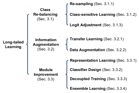
Figure 2: Taxonomy of existing deep long-tailed learning methods.

2 Problem Overview

2.1 Problem Definition

Deep long-tailed learning seeks to learn a deep neural network model from a training dataset with a long-tailed class distribution, where a small fraction of classes have a massive number of samples, and the rest of the classes are associated with only a few samples (c.f. Fig. 1). Let $\{x_{i},y_{i}\}_{i=1}^{n}$ be the long-tailed training set, where each sample $x_{i}$ has a corresponding class label $y_{i}$. The total number of training set over $K$ classes is $n=\sum_{k=1}^{K}n_{k}$, where $n_{k}$ denotes the data number of class $k$; let $\pi$ denote the vector of label frequencies, where $\pi_{k}=n_{k}/n$ indicates the label frequency of class $k$. Without loss of generality, a common assumption in long-tailed learning [31, 32] is that the classes are sorted by cardinality in decreasing order (i.e., if $i_{1}<i_{2}$, then $n_{i_{1}}\geq n_{i_{2}}$, and $n_{1}\gg n_{K}$), and then the imbalance ratio is defined as $n_{1}$/$n_{K}$.

This task is challenging due to two difficulties: (1) imbalanced data numbers across classes make deep models biased to head classes and performs poorly on tail classes; (2) lack of tail-class samples makes it further challenging to train models for tail-class classification. Such a task is fundamental and may occur in various visual recognition tasks, such as image classification [15, 32], detection [19, 33] and segmentation [34, 35, 26].

TABLE I: Statistics of long-tailed datasets. “Cls.” indicates image classification; “Det.” represents object detection; “Seg.” means instance segmentation.

Task	Dataset	$\#$ classes	$\#$ training data	$\#$ test data
Cls.	ImageNet-LT [15]	1,000	115,846	50,000
	CIFAR100-LT [18]	100	50,000	10,000
	Places-LT [15]	365	62,500	36,500
	iNaturalist 2018 [23]	8,142	437,513	24,426
Det./Seg.	LVIS v0.5 [36]	1,230	57,000	20,000
	LVIS v1 [36]	1,203	100,000	19,800
Multi-label Cls.	VOC-LT [37]	20	1,142	4,952
	COCO-LT [37]	80	1,909	5,000
Video Cls.	VideoLT [38]	1,004	179,352	51,244

2.2 Datasets

In recent years, a variety of visual datasets have been released for long-tailed learning, differing in tasks, class numbers and sample numbers. In Table I, we summarize nine visual datasets that are widely used in the deep long-tailed learning community.

In long-tailed image classification, there are four benchmark datasets: ImageNet-LT [15], CIFAR100-LT [18], Places-LT [15], and iNaturalist 2018 [23]. The previous three are sampled from ImageNet [39], CIFAR100 [40] and Places365 [41] following Pareto distributions, respectively, while iNaturalist is a real-world long-tailed dataset. The imbalance ratio of ImageNet-LT, Places-LT and iNaturalist are 256, 996 and 500, respectively; CIFAR100-LT has three variants with various imbalance ratios $\{10,50,100\}$.

In long-tailed object detection and instance segmentation, LVIS [36], providing precise bounding box and mask annotations, is the widely-used benchmark. In multi-label image classification, the benchmarks are VOC-LT [37] and COCO-LT [37], which are sampled from PASCAL VOC 2012 [42] and COCO [43], respectively. Recently, a large-scale “untrimmed” video dataset, namely VideoLT [38], was released for long-tailed video recognition.

2.3 Evaluation Metrics

Long-tailed learning seeks to train a well-performing model on the data with long-tailed class imbalance. To evaluate how well class imbalance is resolved, the model performance on all classes and the performance on class subsets (i.e., head, middle and tail classes) are usually reported. Note that the evaluation metrics should treat each class equally. Following this principle, top-1 accuracy or error rate is often used for balanced test sets, where every test sample is equally important. When the test set is not balanced, mean Average Precision (mAP) or macro accuracy is often adopted since the two metrics treat each class equally. For example, in previous studies, top-1 accuracy or error rate was widely used for long-tailed image classification, in which the test set is usually assumed to be near-balanced. Meanwhile, mAP was adopted for long-tailed object detection, instance segmentation and multi-label image classification, where the test set is usually not balanced.

2.4 Applications

The main applications of deep long-tailed learning include image classification, detection segmentation, and visual relation learning.

Image Classification. The most common applications of long-tailed learning are multi-class classification [15, 32, 44, 45] and multi-label classification [37, 46]. As mentioned in Section 2.2, there are many artificially sampled long-tailed datasets from widely-used multi-class classification datasets (i.e., ImageNet, CIFAR, and Places) and multi-label classification datasets (i.e., VOC and COCO). Based on these datasets, various long-tailed learning methods have been proposed, as shown in Section 3. Besides these artificial tasks, long-tailed learning is also applied to real-world applications, including species classification [23, 24, 47], face recognition [21, 22, 48, 49], face attribute classification [50], cloth attribute classification [50], age classification [51], rail surface defect detection [52], and medical image diagnosis [25, 53]. These real applications usually require more fine-grained discrimination abilities, since the differences among their classes are more subtle. Due to this new challenge, existing deep long-tailed learning methods tend to fail in these applications, since they only focus on addressing the class imbalance and cannot essentially identify subtle class differences. Therefore, when exploring new methods to handle these applications, it is worth considering how to tackle the challenges of class imbalance and fine-grained information identification, simultaneously.

Image Detection / Segmentation. Object detection and instance segmentation has attracted increasing attention in the long-tailed learning community [54, 55, 56, 57, 58, 59], where most existing studies are conducted based on LVIS and COCO. In addition to these widely-used benchmarks, many other applications have also been explored, including urban scene understanding [26, 60] and unmanned aerial vehicle detection [27]. Compared to artificial tasks on LVIS and COCO, these real applications are more challenging due to more complex environments in the wild. For example, the images may be collected from different weather conditions or different times in a day, which may lead to multiple image domains with different data distributions and inconsistent class skewness. When facing these new challenges, existing deep long-tailed learning methods tend to fail. Hence, it is worth exploring how to simultaneously resolve the challenges of class imbalance and domain shifts for handling these applications.

Visual Relation Learning. Visual relation learning is important for image understanding and is attracting rising attention in the long-tailed learning community. Important applications include long-tailed scene graph generation [61, 62], long-tailed visual question answering and image captioning [63, 64]. Most existing long-tailed studies focus on discriminative tasks, so they cannot be applied to the aforementioned applications that require modeling relations between objects or those between images and texts. Even so, it is interesting to explore the high-level ideas (e.g., class re-balancing) in existing long-tailed studies to design application-customized approaches for visual relation learning.

2.5 Relationships with Related Tasks

We then briefly discuss several related tasks, including non-deep long-tailed learning, class-imbalanced learning, few-shot learning, and out-of-domain generalization.

Non-deep long-tailed learning. There are a lot of non-deep learning approaches for long-tailed problems [65, 66, 67]. They usually explore prior knowledge to enhance classic machine learning algorithms for handling the long-tailed problem. For example, the prior of similarity among categories is used to regularize kernel machine algorithm for long-tailed object recognition [65]. Moreover, the prior of a long-tailed power-law distribution produced by the Pitman-Yor Processes (PYP) method [68] is applied to enhance the Bayesian non-parametric framework for long-tailed active learning [66]. An artificial distribution prior is adopted to construct tail-class data augmentation to enhance KNN and SVM for long-tailed scene parsing [67]. Almost all these approaches extract image features based on Scale Invariant Feature Transform (SIFT) [69], Histogram of Gradient Orientation (HOG) [70], or RGB color histogram [71]. Such representation approaches, however, cannot extract highly informative and discriminative features for real visual applications [1] and thus lead to limited performance in long-tailed learning. Recently, in light of the powerful abilities of deep networks for image representation, deep long-tailed methods have achieved significant performance improvement for long-tailed learning. More encouragingly, the use of deep networks also inspires plenty of new solution paradigms for long-tailed learning, such as transfer learning, decoupled training and ensemble learning, which will be introduced in the next section.

Class-imbalanced learning [72, 5] also seeks to train models from class-imbalanced samples. In this sense, long-tailed learning can be regarded as a challenging sub-task of class-imbalanced learning. The dominant distinction is that the classes of long-tailed learning follow a long-tailed class distribution, which is not necessary for class-imbalanced learning. More differences include that in long-tailed learning the number of classes is usually large and the tail-class samples are often very scarce, whereas the number of minority-class samples in class-imbalanced learning is not necessarily small in an absolute sense. These extra challenges lead long-tailed learning to be a more challenging task than class-imbalanced learning. Despite these differences, both seek to resolve the class imbalance, so some high-level solution ideas (e.g., class re-balancing) are shared between them.

Few-shot learning [73, 74, 75, 76] aims to train models from a limited number of labeled samples (e.g., 1 or 5) per class. In this regard, few-shot learning can be regarded as a sub-task of long-tailed learning, in which the tail classes generally have a very small number of samples.

Out-of-domain Generalization [77, 78] indicates a class of tasks, in which the training distribution is inconsistent with the unknown test distribution. Such inconsistency includes inconsistent data marginal distributions (e.g., domain adaptation [79, 80, 81, 82, 83, 84] and domain generalization [85, 86]), inconsistent class distributions (e.g., long-tailed learning [15, 32, 28], open-set learning [87, 88]), and the combination of the previous two situations. From this perspective, long-tailed learning can be viewed as a specific task within out-of-domain generalization.

TABLE II: Summary of existing deep long-tailed learning methods published in the top-tier conferences before mid-2021. There are three main categories: class re-balancing, information augmentation and module improvement. In this table, “CSL” indicates class-sensitive learning; “LA” indicates logit adjustment; “TL” represents transfer learning; “Aug” indicates data augmentation; “RL” indicates representation learning; “CD” indicates classifier design, which seeks to design new classifiers or prediction schemes for long-tailed recognition; “DT” indicates decoupled training, where the feature extractor and the classifier are trained separately; “Ensemble” indicates ensemble learning based methods. In addition, “Target Aspect” indicates from which aspect an approach seeks to resolve the class imbalance. We also make our codebase and our collected long-tailed learning resources available at https://github.com/Vanint/Awesome-LongTailed-Learning.

Method	Year	Class Re-balancing				Augmentation			Module Improvement				Target Aspect
		Re-sampling	CSL	LA		TL	Aug		RL	CD	DT	Ensemble
LMLE [89]	2016								✓				feature
HFL [90]	2016								✓				feature
Focal loss [54]	2017		✓										objective
Range loss [21]	2017								✓				feature
CRL [50]	2017								✓				feature
MetaModelNet [91]	2017					✓
DSTL [92]	2018					✓
DCL [93]	2019	✓											sample
Meta-Weight-Net [94]	2019		✓										objective
LDAM [18]	2019		✓										objective
CB [16]	2019		✓										objective
UML [95]	2019		✓										feature
FTL [96]	2019					✓	✓						feature
Unequal-training [48]	2019								✓				feature
OLTR [15]	2019								✓				feature
Balanced Meta-Softmax [97]	2020	✓	✓										sample, objective
Decoupling [32]	2020	✓	✓						✓	✓	✓		feature, classifier
LST [98]	2020	✓				✓							sample
Domain adaptation [28]	2020		✓										objective
Equalization loss (ESQL) [19]	2020		✓										objective
DBM [22]	2020		✓										objective
Distribution-balanced loss [37]	2020		✓										objective
UNO-IC [99]	2020			✓									prediction
De-confound-TDE [45]	2020			✓						✓			prediction
M2m [100]	2020					✓	✓						sample
LEAP [49]	2020					✓	✓		✓				feature
OFA [101]	2020					✓	✓				✓		feature
SSP [102]	2020					✓			✓				feature
LFME [103]	2020					✓						✓	sample, model
IEM [104]	2020								✓				feature
Deep-RTC [105]	2020									✓			classifier
SimCal [34]	2020										✓	✓	sample, model
BBN [44]	2020											✓	sample, model
BAGS [56]	2020											✓	sample, model
VideoLT [38]	2021	✓											sample
LOCE [33]	2021	✓	✓										sample, objective
DARS [26]	2021	✓	✓			✓							sample, objective
CReST [106]	2021	✓				✓							sample
GIST [107]	2021	✓				✓				✓			classifier
FASA [58]	2021	✓					✓						feature
Equalization loss v2 [108]	2021		✓										objective
Seesaw loss [109]	2021		✓										objective
ACSL [110]	2021		✓										objective
IB [111]	2021		✓										objective
PML [51]	2021		✓										objective
VS [112]	2021		✓										objective
LADE [31]	2021		✓	✓									objective, prediction
RoBal [113]	2021		✓	✓						✓			objective, prediction
DisAlign [29]	2021		✓	✓							✓		objective, classifier
MiSLAS [114]	2021		✓				✓				✓		objective, feature, classifier
Logit adjustment [14]	2021			✓									prediction
Conceptual 12M [115]	2021					✓
DiVE [116]	2021					✓
MosaicOS [117]	2021					✓
RSG [118]	2021					✓	✓						feature
SSD [119]	2021					✓					✓
RIDE [17]	2021					✓						✓	model
MetaSAug [120]	2021						✓						sample
PaCo [121]	2021								✓				feature
DRO-LT [122]	2021								✓				feature
Unsupervised discovery [35]	2021								✓				feature
Hybrid [123]	2021								✓				feature
KCL [13]	2021								✓		✓		feature
DT2 [61]	2021										✓		feature, classifier
LTML [46]	2021											✓	sample, model
ACE [124]	2021											✓	sample, model
ResLT [125]	2021											✓	sample, model
SADE [30]	2021											✓	objective, model

3 Classic Methods

As shown in Fig. 2, we divide existing deep long-tailed learning methods into three main categories according to their main technical characteristics, including class re-balancing, information augmentation, and module improvement. More specifically, class re-balancing consists of three sub-categories: re-sampling, class-sensitive learning (CSL), and logit adjustment (LA). Information augmentation comprises transfer learning (TL) and data augmentation (Aug). Module improvement includes representation learning (RL), classifier design (CD), decoupled training (DT) and ensemble learning (Ensemble). According to this taxonomy, we sort out existing methods in Table II and review them in detail as follows.

3.1 Class Re-balancing

Class re-balancing, a mainstream paradigm in long-tailed learning, seeks to re-balance the negative influence brought by the class imbalance in training sample numbers. This type of methods has three main sub-categories: re-sampling, class-sensitive learning, and logit adjustment. We begin with re-sampling based methods, followed by class-sensitive learning and logit adjustment.

3.1.1 Re-sampling

Conventional training of deep networks is based on mini-batch gradient descent with random sampling, i.e., each sample has an equal probability of being sampled. Such a sampling manner, however, ignores the imbalance issue in long-tailed learning, and naturally samples more head-class samples than tail-class samples in each sample mini-batch. This makes the resulting deep models biased towards head classes and perform poorly on tail classes. To address this issue, re-sampling [126, 127, 128, 129] has been explored to re-balance classes by adjusting the number of samples per class in each sample batch for model training.

In the non-deep learning era, the most classic re-sampling approaches are random over-sampling (ROS) and random under-sampling (RUS). Specifically, ROS randomly repeats the samples from minority classes to re-balance classes before training, while RUS randomly discards the samples from majority classes. When applying them to deep long-tailed learning where the classes are highly skewed, ROS with duplicated tail-class data might lead to overfitting over tail classes, while RUS might discard precious head-class samples and degrade model performance on head classes [44]. Instead of using random re-sampling, recent deep long-tailed studies have developed various class-balanced sampling methods for mini-batch training of deep models.

We begin with Decoupling [32], in which four sampling strategies were evaluated for representation learning of long-tailed data, including random sampling, class-balanced sampling, square-root sampling and progressively-balanced sampling. Specifically, class-balanced sampling means that each class has an equal probability of being selected. Square-root sampling [130] is a variant of class-balanced sampling, where the sampling probability of each class is related to the square root of the sample size in the corresponding class. Progressively-balanced sampling [32] interpolates progressively between random and class-balanced sampling. Based on empirical results, Decoupling [32] found that square-root sampling and progressively-balanced sampling are better strategies for standard model training in long-tailed recognition. The two strategies, however, require knowing the training sample frequencies of different classes in advance, which may be unavailable in real applications.

To address the above issue, recent studies proposed various adaptive sampling strategies. Dynamic Curriculum Learning (DCL) [93] developed a new curriculum strategy to dynamically sample data for class re-balancing. The basic idea is that the more instances from one class are sampled as training proceeds, the lower probability of this class would be sampled in later stages. Following this idea, DCL first conducts random sampling to learn general representations, and then samples more tail-class instances based on the curriculum strategy to handle the imbalance. In addition to using the accumulated sampling times, Long-tailed Object Detector with Classification Equilibrium (LOCE) [33] proposed to monitor model training on different classes via the mean classification prediction score (i.e., running prediction probability), and used this score to guide the sampling rates for different classes. Furthermore, VideoLT [38], focusing on long-tailed video recognition, introduced a new FrameStack method that dynamically adjusts the sampling rates of different classes based on running model performance during training, so that it can sample more video frames from tail classes (generally with lower running performance).

Besides using the statistics computed during model training, some re-sampling approaches resorted to meta learning [131]. Balanced Meta-softmax [97] developed a meta-learning-based sampling method to estimate the optimal sampling rates of different classes for long-tailed learning. Specifically, the developed meta learning method seeks to learn the best sample distribution parameter by optimizing the model classification performance on a balanced meta validation set. Similarly, Feature Augmentation and Sampling Adaptation (FASA) [58] explored the model classification loss on a balanced meta validation set as a score, which is used to adjust the sampling rate for different classes so that the under-represented tail classes can be sampled more.

Note that some long-tailed visual tasks may have multiple levels of imbalance. For example, long-tailed instance segmentation is imbalanced in terms of both images and instances (i.e., the number of instances per image is also imbalanced). To address this task, Simple Calibration (SimCal) [34] proposed a new bi-level class-balanced sampling strategy that combines image-level and instance-level re-sampling for class re-balancing.

Discussions. Re-sampling methods seek to address the class imbalance issue at the sample level. When the label frequencies of different classes are known a priori, progressively-balanced sampling [32] is recommended. Otherwise, using the statistics of model training to guide re-sampling [33] is a preferred solution for real applications. For meta-learning-based re-sampling, it may be difficult to construct a meta validation set in real scenarios. Note that if one re-sampling strategy has already addressed class imbalance well, further using other re-sampling methods may not bring extra benefits. Moreover, the high-level ideas of these re-sampling methods can be applied to design multi-level re-sampling strategies if there are multiple levels of imbalance in real applications.

3.1.2 Class-sensitive Learning

Conventional training of deep networks is based on the softmax cross-entropy loss (c.f. Table III). This loss ignores the class imbalance in data sizes and tends to generate uneven gradients for different classes. That is, each positive sample of one class can be seen as a negative sample for other classes in cross-entropy, which leads head classes to receive more supporting gradients (as they usually are positive samples) and causes tail classes to receive more suppressed gradients (as they usually are negative samples)  [19, 55]. To address this, class-sensitive learning seeks to particularly adjust the training loss values for various classes to re-balance the uneven training effects caused by the imbalance issue [132, 133, 134, 135, 136, 137]. There are two main types of class-sensitive strategies, i.e., re-weighting and re-margining. We begin with class re-weighting as follows.

TABLE III: Summary of losses. In this table, $z$ and $p$ indicate the predicted logits and the softmax probability of the sample $x$, where $z_{y}$ and $p_{y}$ correspond to the class $y$. Moreover, $n$ indicates the total number of training data, where $n_{y}$ is the sample number of the class $y$. In addition, $\pi$ denotes the vector of sample frequencies, where $\pi_{y}\small{=}n_{y}/n$ represents the label frequency of the class $y$. The class-wise weight is denoted by $\omega$ and the class-wise margin is denoted by $\Delta$, if no more specific value is given. Loss-related parameters include $\gamma$.

Loss	Formulation	Type
Softmax loss	${\mathcal{L}_{\rm ce}}=-\log(p_{y})$	-
Focal loss [54]	${\mathcal{L}_{\rm fl}}=-(1-p_{y})^{\gamma}\log(p_{y})$	re-weighting
Weighted Softmax loss	${\mathcal{L}_{\rm wce}}=-\frac{1}{\pi_{y}}\log(p_{y})$	re-weighting
Class-balanced loss [16]	${\mathcal{L}_{\rm cb}}=-\frac{1-\gamma}{1-\gamma^{n_{y}}}\log(p_{y})$	re-weighting
Balanced Softmax loss [97]	${\mathcal{L}_{\rm bs}}=-\log(\frac{\pi_{y}\exp(z_{y})}{\sum_{j}\pi_{j}\exp(z_{j})})$	re-weighting
Equalization loss [19]	${\mathcal{L}_{\rm eq}}=-\log(\frac{\exp(z_{y})}{\sum_{j}\omega_{j}\exp(z_{j})})$	re-weighting
LDAM loss [18]	${\mathcal{L}_{\rm ldam}}=-\log(\frac{\exp(z_{y}-\Delta_{y})}{\sum_{j}\exp(z_{j}-\Delta_{j})})$	re-margining

Re-weighting. To address the class imbalance, re-weighting attempts to adjust the training loss values for different classes by multiplying them with different weights. The most intuitive method is to directly use the label frequencies of training samples for loss re-weighting to re-balance the uneven positive gradients among classes. For example, weighted softmax (c.f. Table III) directly multiplies the loss values of different classes by the inverse of training label frequencies. However, simply multiplying by its inverse may not be the optimal solution. Recent studies thus proposed to tune the influence of training label frequencies based on sample-aware influences [111]. Moreover, Class-balanced loss (CB) [16] introduced a novel concept of effective number to approximate the expected sample number of different classes, which is an exponential function of their training label number. Following this, CB loss enforces a class-balanced re-weighting term, inversely proportional to the effective number of classes, to address the class imbalance (c.f. Table III). Besides the aforementioned re-weighting at the level of log probabilities, we can also use the training label frequencies to re-weight prediction logits. Balanced Softmax [97] proposed to adjust prediction logits by multiplying by the label frequencies, so that the bias of class imbalance can be alleviated by the label prior before computing final losses. Afterwards, Vector-scaling loss (VS) [112] intuitively analyzed the distinct effects of additive and multiplicative logit-adjusted losses, leading to a novel VS loss to combine the advantages of both forms of adjustment.

Instead of using training label frequencies, Focal loss [54] explored class prediction hardness for re-weighting. This is inspired by the observation that class imbalance usually increases the prediction hardness of tail classes, whose prediction probabilities would be lower than those of head classes. Following this, Focal loss uses the prediction probabilities to inversely re-weight classes (c.f. Table III), so that it can assign higher weights to the harder tail classes but lower weights to the easier head classes. Besides using a pre-defined weighting function, the class weights can also be learned from data. For instance, Meta-Weight-Net [94] proposed to learn an MLP-approximated weighting function based on a balanced validation set for class-sensitive learning.

Some recent studies [37, 19] also seek to address the negative gradient over-suppression issue of tail classes. For example, Equalization loss [19] directly down-weights the loss values of tail-class samples when they serve as negative labels for head-class samples. However, simply down-weighting negative gradients may harm the discriminative abilities of deep models. To address this, Adaptive Class Suppression loss (ACSL) [110] uses the output confidence to decide whether to suppress the gradient for a negative label. Specifically, if the prediction probability of a negative label is larger than a pre-defined threshold, it means that the model is confused about this class so the weight for this class is set to 1 to improve model discrimination; otherwise, the weight is set to 0 to avoid negative over-suppression. Moreover, Equalization loss v2 [108] extended the equalization loss [19] by introducing a novel gradient-guided re-weighting mechanism that dynamically up-weights the positive gradients and down-weights the negative gradients for different classes. Similarly, Seesaw loss [109] re-balances positive and negative gradients for each class with two re-weighting factors, i.e., mitigation and compensation. Specifically, to address gradient over-suppression, the mitigation factor alleviates the penalty to tail classes based on a dynamically cumulative sampling number of different classes. Meanwhile, if a false positive sample is observed, the compensation factor up-weights the penalty to the corresponding class for improving model discrimination.

Re-margining. To handle the class imbalance, re-margining attempts to adjust losses by subtracting different margin factors for different classes, so that they have a different minimal margin (i.e., distance) between features and the classifier. Directly using existing soft margin losses [138, 139] is unfeasible, since they ignore the issue of class imbalance. To address this, Label-Distribution-Aware Margin (LDAM) [18] enforces class-dependent margin factors for different classes based on their training label frequencies, which encourages tail classes to have larger margins.

However, the training label frequencies may be unknown in real applications, and simply using them for re-margining also ignores the status of model training on different classes. To address this, recent studies explored various adaptive re-margining methods. Uncertainty-based margin learning (UML) [95] found that the class prediction uncertainty is inversely proportional to the training label frequencies, i.e., tail classes are more uncertain. Inspired by this, UML proposed to use the estimated class-level uncertainty to re-margin losses, so that the tail classes with higher class uncertainty incur a higher loss value and thus have a larger margin between features and the classifier. Moreover, LOCE [33] proposed to use the mean class prediction score to monitor the learning status of different classes and apply it to guide class-level margin adjustment for enhancing tail classes. Domain balancing [22] introduced a novel frequency indicator based on the inter-class compactness of features, and uses this indicator to re-margin the feature space of tail domains. Despite effectiveness, the above re-margining methods for encouraging large tail-class margins may degrade the feature learning of head classes. To address this, RoBal [113] further enforces a margin factor to also enlarge head-class margins.

Discussions. These class-sensitive learning methods aim to resolve the class imbalance issue at the objective level. We summarize some of them in Table III. Both re-weighting and re-margining methods have a similar effect on re-balancing classes. If the negative influence of class imbalance can be addressed by one class-sensitive approach well, it is unnecessary to further apply other class-sensitive methods, which would not bring further performance gain and even harm performance. More specifically, if the training label frequencies are available, directly using them for re-weighting (e.g., Balanced Softmax [97] and VS [112]) or re-margining (e.g., LDAM [18]) provides a simple and generally effective solution for real applications. If not, it is preferred to use the mean class prediction score to guide class-sensitive learning (e.g., ACSL [110] and LOCE [33]) thanks to its simplicity. One can also consider other guidance, like intra-class compactness. However, inter-class compactness of features [22] may be not that informative when the feature dimensions are very high, while the prediction uncertainty [95] may be difficult to estimate accurately in practice. Moreover, using prediction hardness for re-weighting in Focal loss performs well when the number of classes is not large, but may fail when facing a large number of classes. Furthermore, Equalization loss v2, Seesaw loss and RoBal can also be considered if the challenges that they try to resolve appear in real applications.

3.1.3 Logit Adjustment

Logit adjustment [140, 14] seeks to resolve the class imbalance by adjusting the prediction logits of a class-biased deep model. One recent study [14] comprehensively analyzed logit adjustment via training label frequencies of different classes in long-tailed recognition, and theoretically showed that logit adjustment is Fisher consistent to minimize the average per-class error. Following this idea, RoBal [113] applied a post-processing strategy to adjust the cosine classifier based on training label frequencies.

However, the above methods tent to fail when the training label frequencies are unavailable. To address this this, UNO-IC [99] proposed to learn the logit offset based on a balanced meta validation set and use it to calibrate the biased model predictions. Instead of using a meta validation set, DisAlign [29] applied an adaptive calibration function for logit adjustment, where the calibration function is learned by matching the calibrated prediction distribution to a pre-defined relatively balanced class distribution.

The idea of logit adjustment naturally suits agnostic test class distributions. If the test label frequencies are available, LADE [31] proposed to use them to post-adjust model outputs so that the trained model can be calibrated for arbitrary test class distributions. However, the test label frequencies are usually unavailable, which makes LADE less practical in real scenarios.

Discussions. To summarize, these logit adjustment methods address the class imbalance at the prediction level. If the training label frequencies are known, directly using them to post-adjust the predictions of biased deep models is recommended [14, 113]. If such information is unknown, it is preferred to exploit the idea of DisAlign [29] to learn an adaptive calibration function. These logit adjustment methods are exclusive to each other, so using a well-performing one is enough for real applications.

3.1.4 Summary

Class re-balancing is relatively simple among the three main method types of long-tailed learning, but it can achieve comparable or even better performance. Some methods, especially class-sensitive learning, are theoretically inspired or guaranteed to handle long-tailed problems [16, 18, 31]. These advantages enable class re-balancing to be a good candidate for real-world applications.

The ultimate goal of its three sub-categories (i.e., re-sampling, class-sensitive learning and logit adjustment) are the same, i.e., re-balancing classes. Hence, when the class imbalance is not addressed well, combining them may achieve better performance. However, these subtypes are sometimes exclusive to each other. For example, if we have trained a class-balanced deep model via class-sensitive learning, then further using logit adjustment methods to post-adjust model inference will instead lead to biased predictions and suffer poor performance. Therefore, if one wants to combine them, the pipeline should be designed carefully.

One drawback of class re-balancing is that most methods improve tail-class performance at the cost of lower head-class performance, which is like playing on a performance seesaw. Although the overall performance is improved, it cannot essentially handle the issue of lacking information, particularly on tail classes due to limited data sizes. To address this limitation, one feasible solution is to conduct information augmentation as follows.

3.2 Information Augmentation

Information augmentation seeks to introduce additional information into model training, so that the model performance can be improved for long-tailed learning. There are two kinds of methods in this method type: transfer learning and data augmentation.

3.2.1 Transfer Learning

Transfer learning [141, 142, 91, 118, 101] seeks to transfer the knowledge from a source domain (e.g., datasets) to enhance model training on a target domain. In long-tailed learning, there are four main transfer schemes, i.e., model pre-training, knowledge distillation, head-to-tail model transfer, and self-training.

Model pre-training is a popular scheme for deep model training [143, 144, 145, 146, 147] and has also been explored in long-tailed learning. For example, Domain-Specific Transfer Learning (DSTL) [92] first pre-trains the model with all long-tailed samples for representation learning, and then fine-tunes the model on a more class-balanced training subset. In this way, DSTL slowly transfers the learned features to tail classes, obtaining more balanced performance among all classes. Rather than supervised pre-training, Self-supervised Pre-training (SSP) [102] proposed to first use self-supervised learning (e.g., contrastive learning [148] or rotation prediction [149]) for model pre-training, followed by standard training on long-tailed data. Empirical results show self-supervised learning helps to learn a balanced feature space for long-tailed learning [13]. Such a scheme has also been explored to handle long-tailed data with noisy labels [150].

Knowledge distillation seeks to train a student model based on the outputs of a well-trained teacher model [151, 152]. Recent studies have explored knowledge distillation for long-tailed learning. For example, Learning from Multiple Experts (LFME) [103] first trains multiple experts on several less imbalanced sample subsets (e.g., head, middle and tail sets), and then distills these experts into a unified student model. Similarly, Routing Diverse Experts (RIDE) [17] introduced a knowledge distillation method to reduce the parameters of the multi-expert model by learning a student network with fewer experts. Instead of multi-expert teachers, Distill the Virtual Examples (DiVE) [116] showed that learning a class-balanced model as the teacher is also beneficial for long-tailed learning. Following DiVE, Self-Supervision to Distillation (SSD) [119] developed a new self-distillation scheme to enhance decoupled training (c.f. Section 3.3.3). Specifically, SSD first trains a calibrated model based on supervised and self-supervised information via the decoupled training scheme, and then uses the calibrated model to generate soft labels for all samples. Following that, both the generated soft labels and original long-tailed hard labels are used to distill a new student model, followed by a new classifier fine-tuning stage.

Head-to-tail model transfer seeks to transfer the model knowledge from head classes to enhance model performance on tail classes. For example, MetaModelNet [91] proposed to learn a meta-network that can map few-shot model parameters to many-shot model parameters. To this end, MetaModelNet first trains a many-shot model on the head-class training set, and trains a fake few-shot model on a sampled subset from these classes with a very limited number of data to mimic tail classes. Then, the meta-network is learned by mapping the learned fake few-shot model to the many-shot model. Following that, the learned meta-network on head classes is applied to map the true few-shot model trained on tail classes for obtaining better tail-class performance. Instead of model mapping, Geometric Structure Transfer (GIST)  [107] proposed to conduct head-to-tail transfer at the classifier level. Specifically, GIST uses the relatively large classifier geometry information of head classes to enhance the tail-class classifier weights, so that the performance of tail classes can be improved.

Self-training aims to learn well-performing models from a small number of labeled samples and massive unlabeled samples [153, 154, 155]. To be specific, it firstly uses labeled samples to train a supervised model, which is then applied to generate pseudo labels for unlabeled data. Following that, both the labeled and pseudo-labeled samples are used to re-train models. In this way, self-training can exploit the knowledge from massive unlabeled samples to enhance long-tailed learning performance. Such a paradigm, however, cannot be directly used to handle long-tailed problems, because both labeled and unlabeled datasets may follow long-tailed class distributions with different degrees. In such cases, the trained model on labeled samples may be biased to head classes and tends to generate more head-class pseudo labels for unlabeled samples, leading to a more skewed degree of imbalance.

To address this issue, Distribution Alignment and Random Sampling (DARS) [26] proposed to regard the label frequencies of labeled data as a reference and enforce the label frequencies of the generated pseudo labels to be consistent with the labeled ones. Instead of using training label frequencies, Class-rebalancing Self-training (CReST) [106] found that the precision of the supervised model on tail classes is surprisingly high, and thus proposed to select more tail-class samples for online pseudo labeling in each iteration, so that the re-trained model can obtain better performance on tail classes. Beyond classification tasks, MosaicOS [117] resorted to other object-centric images to boost long-tailed object detection. Specifically, it first pre-trains the model with labeled scene-centric images from the original detection dataset, and then uses the pre-trained model to generate pseudo bounding boxes for object-centric images, e.g., ImageNet-1K [39]. After that, MosaicOS fine-tunes the pre-trained model in two stages, i.e., first fine-tuning with the pseudo-labeled object-centric images and then fine-tuning with the original labeled scene-centric images. In this way, MosaicOS alleviates the negative influence of data discrepancies and effectively improves long-tailed performance.

Discussions. These transfer learning methods are complementary to each other, which brings additional information from different perspectives to long-tailed learning. Most of them can be used together for real applications if the resources permit and the combination pipeline is designed well. More concretely, when using model pre-training, the trade-off between supervised discrimination learning and self-supervised class-balanced learning should be tuned [13], which contributes to better long-tailed learning performance. In addition, knowledge distillation with multi-experts can usually achieve better performance than distillation with a single teacher. In head-to-tail model transfer, GIST is a better candidate than MetaModelNet due to its simplicity. Lastly, the use of self-training methods depends on task requirements and what unlabeled samples are available at hand.

3.2.2 Data Augmentation

Data Augmentation aims to enhance the size and quality of datasets by applying pre-defined transformations to each data$/$feature for model training [156, 157]. In long-tailed learning, there are two types of augmentation methods that have been explored, i.e., transfer-based augmentation and non-transfer augmentation.

Head-to-tail transfer augmentation seeks to transfer the knowledge from head classes to augment tail-class samples. For example, Major-to-Minor translation (M2m) [100] proposed to augment tail classes by translating head-class samples to tail-class ones via perturbation-based optimization, which is essentially similar to adversarial attack. The translated tail-class samples are used to construct a more balanced training set for model training.

Besides the data-level transfer in M2m, most studies explore feature-level transfer. For instance, Feature Transfer Learning (FTL) [96] found that tail-class samples have much smaller intra-class variance than head-class samples, leading to biased feature spaces and decision boundaries. To address this, FTL exploits the knowledge of intra-class variance from head classes to guide feature augmentation for tail-class samples, so that the tail-class features have higher intra-class variance. Similarly, LEAP [49] constructs “feature cloud” for each class, and transfers the distribution knowledge of head-class feature clouds to enhance the intra-class variation of tail-class feature clouds. As a result, the distortion of the intra-class feature variance among classes is alleviated, leading to better tail-class performance.

Instead of using the intra-class variation information, Rare-class Sample Generator (RSG) [118] proposed to dynamically estimate a set of feature centers for each class, and use the feature displacement between head-class sample features and their nearest intra-class feature center to augment each tail sample feature for enlarging the tail-class feature space. Moreover, Online Feature Augmentation (OFA) [101] proposed to use class activation maps [158] to decouple sample features into class-specific and class-agnostic ones. Following that, OFA augments tail classes by combining the class-specific features of tail-class samples with class-agnostic features from head-class samples.

Non-transfer augmentation seeks to improve or design conventional data augmentation methods to address long-tailed problems. SMOTE [159], a classic over-sampling method for non-deep class imbalance, can be applied to deep long-tailed problems to generate tail-class samples by mixing several intra-class neighbouring samples. Recently, MiSLAS [114] further investigated data mixup in deep long-tailed learning, and found that (1) data mixup helps to remedy model over-confidence; (2) mixup has a positive effect on representation learning but a negative or negligible effect on classifier learning in the decoupled training scheme [32]. Following these observations, MiSLAS proposed to use data mixup to enhance representation learning in the decoupled scheme. In addition, Remix [160] also resorted to data mixup for long-tailed learning and introduced a re-balanced mixup method to particularly enhance tail classes.

Instead of using data mixup, FASA [58] proposed to generate new data features for each class, based on class-wise Gaussian priors with their mean and variance estimated from previously observed samples. Here, FASA exploits the model classification loss on a balanced validation set to adjust feature sampling rates for different classes, so that the under-represented tail classes can be augmented more than head classes. With a similar idea, Meta Semantic Augmentation (MetaSAug) [120] proposed to augment tail classes with a variant of implicit semantic data augmentation (ISDA) [161]. Specifically, ISDA estimates the class-conditional statistics (i.e., covariance matrices from sample features) to obtain semantic directions, and generates diversified augmented samples by translating sample features along with diverse semantically meaningful directions. To better estimate the covariance matrices for tail classes, MetaSAug explored meta learning to guide the learning of covariance matrices for each class with the class-balanced loss [16], leading to more informative synthetic features.

Discussions. Data augmentation based methods attempt to address the class imbalance at the sample or feature levels. The goals of these methods are consistent, so they can be used simultaneously if the combination pipeline is constructed well. Among its two subtypes, head-to-tail transfer augmentation is more intuitive than non-transfer augmentation. More specifically, head-to-tail transfer at the feature level (e.g., RSG) seems to perform better than transfer at the sample level (e.g., M2m). In the feature-level transfer augmentation, RSG is preferred thanks to its easy-to-use source code, whereas the intra-class variation in FTL and LEAP may be less informative for augmentation when the feature dimension is very high. In non-transfer augmentation, mixup-based strategies are usually used thanks to their simplicity, where MiSLAS has demonstrated promising performance. In contrast, the class-wise Gaussian priors in FASA and the covariance matrices in MetaSAug may be difficult to estimate in various real scenarios.

3.2.3 Summary

Information augmentation addresses the long-tailed problems by introducing additional knowledge, and thus is compatible with and complementary to other two method types, i.e., class re-balancing and module improvement. For the same reason, its two method subtypes, i.e., transfer learning and data augmentation, are also complementary to each other. More concretely, both the subtypes are able to improve tail-class performance without sacrificing head-class performance if designed carefully. Considering that all classes are important in long-tailed learning, this type of method is worth further exploring. Moreover, data augmentation is a very fundamental technique and can be used for a variety of long-tailed problems, which makes it more practical than other paradigms in real-world applications. However, simply using existing class-agnostic augmentation techniques for improving long-tailed learning is unfavorable, since they ignore the class imbalance and inevitably augment more head-class samples than tail-class samples. How to better conduct data augmentation for long-tailed learning is still an open question.

3.3 Module Improvement

Besides re-balancing and information augmentation, researchers also explored methods to improve network modules in long-tailed learning. These methods can be divided into four categories: (1) representation learning improves the feature extractor; (2) classifier design enhances the model classifier; (3) decoupled training aims to boost the learning of both the feature extractor and the classifier; (4) ensemble learning improves the whole architecture.

3.3.1 Representation Learning

Existing long-tailed learning methods improve representation learning based on three main paradigms, i.e., metric learning, prototype learning, and sequential training.

Metric learning aims at designing task-specific distance metrics for establishing similarity or dissimilarity between data. In deep long-tailed learning, metric learning based methods seek to explore various distance-based losses to learn a discriminative feature space for long-tailed data. One example is Large Margin Local Embedding (LMLE) [89], which introduced a quintuplet loss to learn representations that maintain both inter-cluster and inter-class margins. Unlike the triplet loss [162] that samples two contrastive pairs, LMLE presented a quintuplet sampler to sample four contrastive pairs, including a positive pair and three negative pairs. The positive pair is the most distant intra-cluster sample, while the negative pairs include two inter-clusters samples from the same class (one is the nearest and one is the most distant within the same cluster) and the nearest inter-class sample. Following that, LMLE introduced a quintuplet loss to encourage the sampled quintuplet to follow a specific distance order. In this way, the learned representations preserve not only locality across intra-class clusters but also discrimination between classes. Moreover, each data batch contains the same number of samples from different classes for class re-balancing. However, LMLE does not consider the sample differences among head and tail classes. To address this, Class Rectification Loss (CRL) [50] explored hard pair mining and proposed to construct more hard-pair triplets for tail classes, so that tail-class features can have a larger degree of intra-class compactness and inter-class distances.

Rather than sampling triplets or quintuplets, range loss [21] innovated representation learning by using the overall distances among all sample pairs within one mini-batch. In other words, the range loss uses statistics over the whole batch and thus alleviates the bias of data number imbalance over classes. Specifically, range loss enlarges the inter-class distance by maximizing the distances of any two class centers within the mini-batch, and reduces the intra-class variation by minimizing the largest distances between intra-class samples. In this way, the range loss obtains features with better discriminative abilities and less imbalanced bias.

Recent studies also explored contrastive learning for long-tailed problems. KCL [13] proposed a $k$-positive contrastive loss to learn a balanced feature space, which helps to alleviate the class imbalance and improve model generalization. Parametric contrastive learning (PaCo) [121] further innovated supervised contrastive learning by adding a set of parametric learnable class centers, which plays the same role as a classifier if regarding the class centers as the classifier weights. Following that, Hybrid [123] introduced a prototypical contrastive learning strategy to enhance long-tailed learning. DRO-LT [122] extended the prototypical contrastive learning with distribution robust optimization [163], which makes the learned model more robust to distribution shift.

Prototype learning based methods seek to learn class-specific feature prototypes to enhance long-tailed learning performance. Open Long-Tailed Recognition (OLTR) [15] innovatively explored the idea of feature prototypes to handle long-tailed recognition in an open world, where the test set also includes open classes that do not appear in training data. To address this task, OLTR maintains a visual meta memory containing discriminative feature prototypes, and uses the features sampled from the visual memory to augment the original features for better discrimination. Meanwhile, the sample features from novel classes are enforced to be far away from the memory and closer to the origin point. In this way, the learned feature space enables OLTR to classify all seen classes and detect novel classes. However, OLTR only maintains a static prototype memory and each class has only one prototype. Such a single prototype per class may fail to represent the real data distribution. To address this issue, Inflated Episodic Memory (IEM) [104] further innovated the meta-embedding memory by a dynamical update scheme, in which each class has independent and differentiable memory blocks. Each memory block is updated to record the most discriminative feature prototypes of the corresponding categories, thus leading to better performance than OLTR.

Sequential training based methods learn data representation in a continual way. For example, Hierarchical Feature Learning (HFL) [90] took inspiration from that each class has its individuality in discriminative visual representation. Therefore, HFL hierarchically clusters objects into visually similar class groups, forming a hierarchical cluster tree. In this cluster tree, the model in the original node is pre-trained on ImageNet-1K; the model in each child node inherits the model parameters from its parent node and is then fine-tuned based on samples in the cluster node. In this way, the knowledge from the groups with massive classes is gradually transferred to their sub-groups with fewer classes. Similarly, Unequal-training [48] proposed to divide the dataset into head-class and tail-class subsets, and treat them differently in the training process. First, unequal-training uses the head-class samples to train relatively discriminative and noise-resistant features with a new noise-resistant loss. After that, it uses tail-class samples to enhance the inter-class discrimination of representations via hard identity mining and a novel center-dispersed loss.

Discussions. These representation learning methods seek to address the class imbalance at the feature level. The methods within each subtype are competing with each other (e.g., KCL [13] vs PaCo [121] and OLTR [15] vs IEM [104]), while the methods from different subtypes may be complementary to each other (e.g., KCL [13] and Unequal-training [48]). Therefore, the pipeline must be carefully designed, if one wants to combine them together. Moreover, when handling real long-tailed applications, PaCo [121] is recommended to use thanks to its promising performance and open-source code. If there are open classes in test data, IEM [104] is preferred. Other methods, like Unequal-training [48], can also be considered if they suit real scenarios.

3.3.2 Classifier Design

In addition to representation learning, researchers also explored different types of classifiers to address long-tailed problems. In generic visual problems [10, 148], the common practice of deep learning is to use linear classifier $p=\phi(w^{\top}f\small{+}b)$, where $\phi$ denotes the softmax function and the bias term $b$ can be discarded. However, long-tailed class imbalance often results in larger classifier weight norms for head classes than tail classes [96], which makes the linear classifier easily biased to dominant classes.

To address this, recent studies [49, 113] proposed to use the scale-invariant cosine classifier $p=\phi((\frac{w^{\top}f}{\|w\|\|f\|})/\tau+b)$, where both the classifier weights and sample features are normalized. Here, the temperature $\tau$ should be chosen reasonably [164], or the classifier performance would be negatively influenced. However, normalizing the feature space may harm its representation abilities. Therefore, the $\tau$-normalized classifier [32] rectifies the imbalance by only adjusting the classifier weight norms through a $\tau$-normalization procedure. Formally, let $\tilde{w}=\frac{w}{\|w\|^{\tau}_{2}}$, where $\tau$ is the temperature factor for normalization. When $\tau=1$, the $\tau$-normalization reduces to $L_{2}$ normalization, while when $\tau=0$, no scaling is imposed. Note that, the hyper-parameter $\tau$ can also be trained with class-balanced sampling, and the resulting classifier is named the learnable weight scaling classifier [32]. Another approach to address classifier weight imbalance is to use the nearest class mean classifier [32], which first computes the mean features for each class on the training set as the classifier, and then conducts prediction based on the nearest neighbor algorithm [165].

There are also some more complicated classifier designs based on hierarchical classification, causal inference or classifier knowledge transfer. For example, Realistic Taxonomic Classifier (RTC) [105] proposed to address class imbalance with hierarchical classification by mapping images into a class taxonomic tree structure, where the hierarchy is defined by a set of classification nodes and node relations. Different samples are adaptively classified at different hierarchical levels, where the level at which the prediction is made depends on the sample classification difficulty and the classifier confidence. Such a design favors correct decisions at intermediate levels rather than incorrect decisions at the leaves.

Causal classifier [45] resorted to causal inference for keeping the good and removing the bad momentum causal effects in long-tailed learning. The good causal effect indicates the beneficial factor that stabilizes gradients and accelerates training, while the bad causal effect indicates the accumulated long-tailed bias that leads to poor tail-class performance. To better approximate the bias information, the causal classifier applies a multi-head strategy to divide the channel (or dimensions) of model weights and data features equally into $K$ groups. Formally, the causal classifier calculates the original logits by $p=\phi(\frac{\tau}{K}\sum_{k=1}^{K}\frac{(w^{k})^{\top}f^{k}}{(\|w^{k}\|+\gamma)\|f^{k}\|})$, where $\tau$ is the temperature factor and $\gamma$ is a hyper-parameter. This classifier is essentially the cosine classifier when $\gamma=0$. In inference, the causal classifier removes the bad causal effect by subtracting the prediction when the input is null, i.e., $p=\phi(\frac{\tau}{K}\sum_{k=1}^{K}\frac{(w^{k})^{\top}f^{k}}{(\|w^{k}\|+\gamma)\|f^{k}\|}-\alpha\frac{cos(x^{k},\hat{d}^{k})(w^{k})^{\top}\hat{d}^{k}}{\|w^{k}\|+\gamma})$, where $\hat{d}$ is the unit vector of the exponential moving average features, and $\alpha$ is a trade-off parameter to control the direct and indirect effects. More intuitively, the classifier records the bias by computing the exponential moving average features during training, and then removes the bad causal effect by subtracting the bias from prediction logits during inference.

GIST classifier [107] seeks to transfer the classifier geometric structure of head classes to tail classes. Specifically, the GIST classifier consists of a class-specific weight center (for encoding the class location) and a set of displacements (for encoding the class geometry). By exploiting the relatively large displacements from head classes to enhance tail-class weight centers, the GIST classifier is able to obtain better performance on tail classes.

(a) Standard training

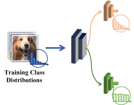
(b) BBN [44], TLML [46], SimCAL [34]

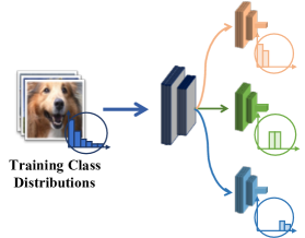
(c) BAGS [56], LFME [103]

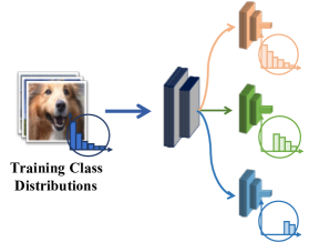
(d) ACE [124], ResLT [125]

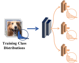
(e) RIDE [17]

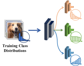
(f) SADE [30]

Figure 3: Illustrations of existing ensemble-based long-tailed methods. Compared to standard training (a), the trained experts by ensemble-based methods (b-f) may have different expertise, e.g., being skilled in different class distributions or different class subsets (indicated by different colors). For example, BBN and SimCAL train two experts for simulating the original long-tailed and uniform distributions so that they can address the two distributions well. BAGS, LFME, ACE, and ResLT train multiple experts by sampling class subsets, so that different experts can particularly handle different sets of classes. SADE directly trains multiple experts to separately simulate long-tailed, uniform and inverse long-tailed class distributions from a stationary long-tailed distribution, which enables it to handle test sets with agnostic class distributions based on self-supervised aggregation.

Discussions. These methods address the imbalance at the classifier level. Note that these classifiers are exclusive to each other, and the choice of classifiers also influences other long-tailed methods. For example, the effects of data mixup are different for the linear classifier and the cosine classifier. Hence, when exploring new long-tailed approaches, it is better to first determine which classifier is used. Generally, the cosine classifier or the learnable weight-scaling classifier are recommended, as they are empirically robust to the imbalance and also easy to use. Moreover, when designing feature prototype-based methods, the nearest class mean classifier is a good choice. More complicated classifier designs (e.g., RTC, Causal and GIST) can also be considered if real applications are complex and hard to handle.

3.3.3 Decoupled Training

Decoupled training decouples the learning procedure into representation learning and classifier training. Here, decoupled training represents a general paradigm for long-tailed learning instead of a specific approach. Decoupling [32] was the pioneering work to introduce such a two-stage decoupled training scheme. It empirically evaluated different sampling strategies (mentioned in Section 3.1.1) for representation learning in the first stage, and then evaluated different classifier training schemes by fixing the trained feature extractor in the second stage. In the classifier learning stage, there are also four methods, including classifier re-training with class-balanced sampling, the nearest class mean classifier, the $\tau$-normalized classifier, and the learnable weight-scaling classifier. The main observations are twofold: (1) random sampling is surprisingly the best strategy for representation learning in decoupled training; (2) re-adjusting the classifier leads to significant performance improvement in long-tailed recognition.

Following this scheme, KCL [13] empirically observed that a balanced feature space is beneficial to long-tailed learning. Therefore, it innovated the decoupled training scheme by developing a $k$-positive contrastive loss to learn a more class-balanced and class-discriminative feature space, which leads to better long-tailed learning performance. Moreover, MiSLAS [114] empirically observed that data mixup is beneficial to features learning but has a negative/negligible effect on classifier training under the two-stage decoupled training scheme. Therefore, MiSLAS proposed to enhance the representation learning with data mixup in the first stage, while applying a label-aware smoothing strategy for better classifier generalization in the second stage.

Several recent studies particularly enhanced the classifier training stage. For example, OFA [101] innovated the classifier re-training through tail-class feature augmentation. SimCal [34] enhanced the classifier training stage by calibrating the classification head with a novel bi-level class-balanced sampling strategy for long-tailed instance segmentation. DisAlign [29] innovated the classifier training with a new adaptive logit adjustment strategy. Very recently, DT2 [61] applied the scheme of decoupled training to the scene graph generation task, which demonstrates the effectiveness of decoupled training in handling long-tailed visual relation learning.

Discussions. Decoupled training methods resolve the class imbalance issue at both the feature and classifier levels. Under ideal conditions, combining different methods can lead to better long-tailed performance, e.g., using self-supervised pre-training [13] and mixup augmentation [114] together for better representation learning, and applying label-aware smoothing [114] and tail-class feature augmentation [101] together for better classifier tuning. Therefore, it is recommended to use MiSLAS [114] as a base method and use different tricks on it. Note that some representation methods are also competing to each other, e.g., different sampling methods for representation learning [32].

The classifier learning stage does not introduce too many computation costs but can lead to significant performance gains. This makes decoupled training attract increasing attention. One critique is that the accumulated training stages make decoupled training less practical to be integrated with existing well-formulated methods for other long-tailed problems like object detection and instance segmentation. Despite this, the idea of decoupled training is conceptually simple and thus can be easily used to design new methods for resolving various long-tailed problems, like DT2 [61].

3.3.4 Ensemble Learning

Ensemble learning based methods strategically generate and combine multiple network modules (namely, multiple experts) to solve long-tailed visual learning problems. We summarize the main schemes of existing ensemble-based methods in Fig. 3, which will be detailed as follows.

BBN [44] proposed to use two network branches, i.e., a conventional learning branch and a re-balancing branch (cf. Table 3(b)), to handle long-tailed recognition. To be specific, the conventional learning branch applies uniform sampling to simulate the original long-tailed training distribution, while the re-balancing branch applies a reversed sampler to sample more tail-class samples in each mini-batch for improving tail-class performance. The predictions of two branches are dynamically combined during training, so that the learning focus of BBN gradually changes from head classes to tail classes. Following BBN, LTML [46] applied the bilateral-branch network scheme to solve long-tailed multi-label classification. To be specific, LTML trains each branch using the sigmoid cross-entropy loss for multi-label classification and enforces a logit consistency loss to improve the consistency of the two branches. Similarly, SimCal [34] explored a dual classification head scheme, a conventional classification head and a calibrated classification head, to address long-tail instance segmentation. Based on a new bi-level sampling strategy, the calibrated classification head is able to improve the performance on tail classes, while the original head aims to maintain the performance on head classes.

Instead of bilateral branches, BAGS [56] explored a multi-head scheme to address long-tailed object detection. Specifically, BAGS took inspiration from an observation that learning a more uniform distribution with fewer samples is sometimes easier than learning a long-tailed distribution with more samples. Therefore, BAGS divides classes into several groups, where the classes in each group have a similar number of training data. Then, BAGS applies multiple classification heads for prediction, where different heads are trained on different class groups (cf. Table 3(c)). In this way, each classification head performs the softmax operation on classes with a similar number of training data, thus avoiding the negative influence of class imbalance. Moreover, BAGS also introduces a label of “other classes” into each group to alleviate the contradiction among different heads. Similar to BAGS, LFME [103] divides the long-tailed dataset into several subsets with smaller class imbalance degrees, and trains multiple experts with different sample subsets. Based on these experts, LFME then learns a unified student model using adaptive knowledge distillation from multiple teachers.

Instead of division into several balanced sub-groups, ACE [124] divides classes into several skill-diverse subsets: one subset contains all classes; one contains middle and tail classes; another one has only tail classes (cf. Table 3(d)). ACE then trains multiple experts with various class subsets, so that different experts have specific and complementary skills. Moreover, considering that various subsets have different sample numbers, ACE also applies a distributed-adaptive optimizer to adjust the learning rate for different experts. A similar idea of ACE was also explored in ResLT [125].

Instead of dividing the dataset, RIDE [17] uses all training samples to train multiple experts with softmax loss respectively (cf. Table 3(e)), and enforces a KL-divergence based loss to improve the diversity among various experts. Following that, RIDE applies an expert assignment module to improve computing efficiency. Note that training each expert with the softmax loss independently boosts the ensemble performance on long-tailed learning a lot. However, the learned experts by RIDE are not diverse enough.

Self-supervised Aggregation of Diverse Experts (SADE) [30] explored a new multi-expert scheme to handle test-agnostic long-tailed recognition, where the test class distribution can be either uniform, long-tailed or even inversely long-tailed. To be specific, SADE developed a novel spectrum-spanned multi-expert framework (cf. Table 3(f)), and innovated the expert training scheme by introducing diversity-promoting expertise-guided losses that train different experts to handle different class distributions, respectively. In this way, the learned experts are more diverse than RIDE, leading to better ensemble performance, and integratedly span a wide spectrum of possible class distributions. In light of this, SADE further introduced a self-supervised learning method, namely prediction stability maximization, to adaptively aggregate experts at test time for better handling unknown test class distribution.

Discussions. These ensemble-based methods address the class imbalance at the model level. As they require particular manners for multi-model design and training (cf. Fig. 3), they are exclusive to each other and usually cannot be used together. More specifically, the methods with bilateral branches like BBN and TLML only have two experts, whose empirical performance has been shown worse than the approaches with more experts. Moreover, the methods with experts trained on class subsets like BAGS and ACE may suffer from expert inconsistency in terms of different label spaces, which makes the aggregation of experts difficult and may lead to poor performance in real applications. Instead, RIDE trains multiple experts with all samples but the resulting multiple experts are not diverse enough. In contrast, SADE is able to train skill-diverse experts with the same label space, and thus is recommended for real applications. One concern of these ensemble-based methods is that they generally lead to higher computational costs due to the use of multiple experts. Such a concern, however, can be alleviated by using a shared feature extractor. Moreover, efficiency-oriented expert assignment and knowledge distillation strategies [103, 17] can also reduce computational complexity.

3.3.5 Summary

Module improvement based methods seek to address long-tailed problems by improving network modules. Specifically, representation learning and classifier design are fundamental problems of deep learning, being worth further exploring for long-tailed problems. Both representation learning and classifier design are complementary to decoupled training. The scheme of decoupled training is conceptually simple and can be easily used to design new methods for resolving real long-tailed applications. In addition, ensemble-based methods, thanks to the aggregation of multiple experts, are able to achieve better long-tailed performance without sacrificing the performance on any class subsets, e.g., head classes. Since all classes are important, such a superiority enables ensemble-based methods to be a better choice for real applications compared to existing class re-balancing methods that usually improve tail-class performance at the cost of lower head-class performance. Here, both ensemble-based methods and decoupled training require specific model training and design manners, so it is not easy to use them together unless very careful design.

Note that most module improvement methods are developed based on fundamental class re-balancing methods. Moreover, module improvement methods are complementary to information augmentation methods. Using them together can usually achieve better performance for real-world long-tailed applications.

4 Empirical Studies

This section empirically analyzes existing long-tailed learning methods. To begin with, we introduce a new evaluation metric.

4.1 Novel Evaluation Metric

The key goal of long-tailed learning is to handle the class imbalance for better model performance. Therefore, the common evaluation protocol [22, 13] is directly using the top-1 test accuracy (denoted by $A_{t}$) to judge how well long-tailed methods perform and which method handles class imbalance better. Such a metric, however, cannot accurately reflect the relative superiority among different methods when handling class imbalance, as the top-1 accuracy is also influenced by other factors apart from class imbalance. For example, long-tailed methods like ensemble learning (or data augmentation) also improve the performance of models, trained on a balanced training set. In such cases, it is hard to tell if the performance gain is from the alleviation of class imbalance or from better network architectures (or more data information).

To better evaluate the method effectiveness in handling class imbalance, we explore a new metric, namely relative accuracy $A_{r}$, to alleviate the influence of unnecessary factors in long-tailed learning. To this end, we first compute an empirically upper reference accuracy $A_{u}=\max(A_{v},A_{b})$, which is the maximal value between the vanilla accuracy $A_{v}$ of the backbone trained on a balanced training set with cross-entropy and the balanced accuracy $A_{b}$ of the model trained on a balanced training set with the corresponding long-tailed method. Here, the balanced training set is a variant of the long-tailed training set, where the total data number is similar but each class has the same number of data. This upper reference accuracy, obtained from the balanced training set, is used to alleviate the influence apart from class imbalance, and then the relative accuracy is defined by $A_{r}=\frac{A_{t}}{A_{u}}$. Note that this metric is mainly designed for empirical understanding, i.e., to evaluate to what extent existing methods resolve the class imbalance. We conduct this analysis based on the ImageNet-LT dataset [15], where a corresponding balanced training set variant can be built by sampling from the original ImageNet following [13].

4.2 Experimental Settings

We then introduce the experimental settings.

Datasets. We adopt the widely-used ImageNet-LT [15] and iNaturalist 2018 [23] as the benchmark long-tailed dataset for empirical studies. Their dataset statistics can be found in Table I. Besides the performance regarding all classes, we also report performance on three class subsets: Head (more than 100 images), Middle (20$\sim$100 images) and Tail (less than 20 images).

Baselines. We select long-tailed methods via two criteria: (1) the source codes are publicly available or easy to re-implement; (2) the methods are evaluated on ImageNet-LT in the corresponding papers. As a result, more than 20 methods are empirically evaluated in this paper, including baseline (Softmax), class-sensitive learning (Weighted Softmax, Focal loss [54], LDAM [18], ESQL [19], Balanced Softmax [97], LADE [31]), logit adjustment (UNO-IC [99]), transfer learning (SSP [102]), data augmentation (RSG [118]) representation learning (OLTR [15], PaCo [121]). classifier design (De-confound [45]), decoupled training (Decouple-IB-CRT [32], CB-CRT [32], SR-CRT [32], PB-CRT [32], MiSLAS [114]), ensemble learning (BBN [44], LFME [103], RIDE [17], ResLT [125], SADE [30]).

Implementation details. We implement all experiments in PyTorch. Following [31, 17, 32], we use ResNeXt-50 for ImageNet-LT and and ResNet-50 for iNaturalist 2018 as the network backbones for all methods. We conduct model training with the SGD optimizer based on batch size 256, momentum 0.9 and weight decay factor 0.0005, and learning rate 0.1 (linear LR decay). For method-related hyper-parameters, we set the values by either directly following the original papers or manual tuning if the default values perform poorly. Moreover, we use the same basic data augmentation (i.e., random resize and crop to 224, random horizontal flip, color jitter, and normalization) for all methods.

4.3 Results on ImageNet-LT

Observations on all classes. Table V and Fig. 4 report the average performance of ImageNet-LT over all classes. From these results, we have several observations on the overall method progress and different method types. As shown in Table V, almost all long-tailed methods perform better than the Softmax baseline in terms of accuracy, which demonstrates the effectiveness of long-tailed learning. Even so, there are two methods performing slightly worse than Softmax, i.e., Decouple-CB-CRT [32] and BBN [44]. We speculate that the poor performance of Decouple-CB-CRT results from poor representation learning by class-balanced sampling in the first stage of decoupled training (refer to [32] for more empirical observations). The poor results of BBN (based on the official codes) may come from the cumulative learning strategy, which gradually adjusts the learning focus from head classes to tail classes; at the end of the training, however, it may put too much focus on the tail ones. As a result, despite the better tail-class performance, the model accuracy on head classes drops significantly (c.f. Table V), leading to worse average performance.

In addition to accuracy, we also evaluate long-tailed methods based on upper reference accuracy (UA) and relative accuracy (RA). Table V shows that most methods have the same UA as the baseline model, but there are still some methods having higher UA, e.g., SSP, MiSLAS, and SADE. For these methods, the performance improvement comes not only from the alleviation of class imbalance, but also from other factors, like data augmentation or better network architectures. Therefore, simply using accuracy for evaluation is not comprehensive enough, while the proposed RA metric provides a good complement as it alleviates the influences of factors apart from class imbalance. For example, MiSLAS, based on data mixup, has higher accuracy than Balanced Softmax under 90 training epochs, but it also has higher UA. As a result, the relative accuracy of MiSLAS is lower than Balanced Softmax, which means that Balanced Softmax alleviates class imbalance better than MiSLAS under 90 training epochs.

Although some recent high-accuracy methods have lower RA, the overall development trend of long-tailed learning is still positive, as shown in Fig. 4. Such a performance trend demonstrates that recent studies of long-tailed learning make real progress. Moreover, the RA of the state-of-the-art SADE is 93.0, which implies that there is still room for improvement in the future.

TABLE IV: Results on ImageNet-LT in terms of accuracy (Acc), upper reference accuracy (UA), relative accuracy (RA) under 90 or 200 training epochs. In this table, CR, IA and MI indicate class re-balancing, information augmentation and module improvement, respectively.

Type	Method	90 epochs				200 epochs
		Acc	UA	RA		Acc	UA	RA
Baseline	Softmax	45.5	57.3	79.4		46.8	57.8	81.0
CR	Weighted Softmax	47.9	57.3	83.6		49.1	57.8	84.9
	Focal loss [54]	45.8	57.3	79.9		47.2	57.8	81.7
	LDAM [18]	51.1	57.3	89.2		51.1	57.8	88.4
	ESQL [19]	47.3	57.3	82.5		48.0	57.8	83.0
	UNO-IC [99]	45.7	57.3	81.4		46.8	58.6	79.9
	Balanced Softmax [97]	50.8	57.3	88.7		51.2	57.8	88.6
	LADE [31]	51.5	57.8	89.1		51.6	57.8	89.3
IA	SSP [102]	53.1	59.6	89.1		53.3	59.9	89.0
	RSG [118]	49.6	57.3	86.7		52.9	57.8	91.5
MI	OLTR [15]	46.7	57.3	81.5		48.0	58.4	82.2
	PaCo [121]	52.7	58.7	89.9		54.4	59.6	91.3
	De-confound [45]	51.8	57.7	89.8		51.3	57.8	88.8
	Decouple-IB-CRT [32]	49.9	57.3	87.1		50.3	58.1	86.6
	Decouple-CB-CRT [32]	44.9	57.3	78.4		43.0	57.8	74.4
	Decouple-SR-CRT [32]	49.3	57.3	86.0		48.5	57.8	83.9
	Decouple-PB-CRT [32]	48.4	57.3	84.5		48.1	57.8	83.2
	MiSLAS [114]	51.4	58.3	88.2		53.4	59.7	89.4
	BBN [44]	41.2	57.3	71.9		44.7	57.8	77.3
	LFME [103]	47.0	57.3	82.0		48.0	57.8	83.0
	ResLT [125]	51.6	57.3	90.1		53.2	58.1	91.6
	RIDE [17]	55.5	60.2	92.2		56.1	60.9	92.1
	SADE [30]	57.3	61.9	92.6		58.8	63.2	93.0

TABLE V: Accuracy results on ImageNet-LT regarding head, middle and tail classes under 90 or 200 training epochs. In this table, WS indicates weighed softmax and BS indicates balanced softmax. The types of methods are the same to Table V.

Method	90 epochs				200 epochs
	Head	Middle	Tail		Head	Middle	Tail
Softmax	66.5	39.0	8.6		66.9	40.4	12.6
WS	66.3	42.2	15.6		57.9	46.2	34.0
Focal loss [54]	66.9	39.2	9.2		67.0	41.0	13.1
LDAM [18]	62.3	47.4	32.5		60.0	49.2	31.9
ESQL [19]	62.5	44.0	15.7		63.1	44.6	17.2
UNO-IC [99]	66.3	38.7	9.3		67.0	40.3	12.7
BS [97]	61.7	48.0	29.9		62.4	47.7	32.1
LADE [31]	62.2	48.6	31.8		63.1	47.7	32.7
SSP [102]	65.6	49.6	30.3		67.3	49.1	28.3
RSG [118]	68.7	43.7	16.2		65.0	49.4	31.1
OLTR [15]	58.2	45.5	19.5		62.9	44.6	18.8
PaCo [121]	59.7	51.7	36.6		63.2	51.6	39.2
De-confound [45]	63.0	48.5	31.4		64.9	46.9	28.1
IB-CRT [32]	62.6	46.2	26.7		64.2	46.1	26.0
CB-CRT [32]	62.4	39.3	14.9		60.9	36.9	13.5
SR-CRT [32]	64.1	43.9	19.5		66.0	42.3	18.0
PB-CRT [32]	63.9	45.0	23.2		64.9	43.1	20.6
MiSLAS [114]	62.1	48.9	32.6		65.3	50.6	33.0
BBN [44]	40.0	43.3	40.8		43.3	45.9	43.7
LFME [103]	60.6	43.5	22.0		64.1	42.3	22.8
ResLT [125]	57.8	50.4	40.0		61.6	51.4	38.8
RIDE [17]	66.9	52.3	34.5		67.9	52.3	36.0
SADE [30]	65.3	55.2	42.0		67.2	55.3	40.0

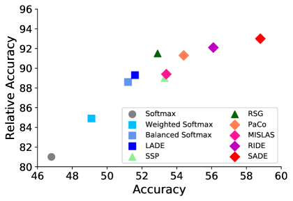
Figure 4: Performance trends of long-tailed learning methods in terms of accuracy and relative accuracy under 200 epochs. Here, the shape of $\circ$ indicates the softmax baseline; $\square$ indicates class re-balancing; $\bigtriangleup$ and $\diamondsuit$ are information augmentation and module improvement methods, respectively. Different colors represent different methods.

We also evaluate the influence of different training epochs (i.e., 90 and 200) in Table V. Overall, training with 200 epochs leads to better performance for most long-tailed methods, because sufficient training enables deep models to fit data better and learn better visual representations. However, there are also some methods that perform better when only training 90 epochs, e.g., De-confound and Decouple-CB-CRT. We speculate that, for these methods, 90 epochs are enough to train models well, while training more epochs does not bring additional benefits but increases the training difficulties since it also influences the learning rate decay scheme.

Observations on different method types. We next analyze different method types in Table V. To begin with, almost all class re-balancing (CR) methods all beneficial to long-tailed learning performance, compared to the baseline model. Among them, LADE, Balanced Softmax and LDAM achieve state-of-the-art. Moreover, Focal loss was initially proposed to handle object detection [54]. However, when handling a highly large number of classes (e.g., 1,000 in ImageNet-LT), Focal loss cannot perform well and only leads to marginal improvement. In LDAM, there is a deferred re-balancing optimization schedule in addition to the LDAM loss. Simply learning with the LDAM loss without the deferred scheme cannot achieve promising results. In addition, as shown in Table V, the upper reference accuracy of most class-sensitive methods is the same, so their relative accuracy is positively correlated to accuracy. Hence, the accuracy improvement in this method type can accurately reflect the alleviation of class imbalance.

In information augmentation (IA), both SSP (transfer learning) and RSG (data augmentation) help to handle long-tailed imbalance. Although SSP also improves upper reference accuracy, its relative accuracy is increased more significantly, implying that the performance gain mostly comes from handling the class imbalance. In module improvement (MI), all methods contribute to addressing the imbalance. By now, the state of the art is ensemble-based long-tailed methods, i.e., SADE and RIDE, in terms of both accuracy and relative accuracy. Although ensemble learning also improves upper reference accuracy, the performance gain from handling imbalance is more significant, leading to higher relative accuracy.

Results on different class subsets. We then report the performance in terms of different class subsets. As shown in Table V, almost all methods improve tail-class and middle-class performance at the cost of lower head-class performance. The head classes, however, are also important in long-tailed learning, so it is necessary to improve long-tailed performance without sacrificing the performance of the head. Potential solutions include information augmentation and ensemble learning, e.g., SSP and SADE. By comparing both Tables V and V, one can find that the overall performance gain largely depends on the improvement of middle and tail classes; hence, how to improve their performance is still the most important goal of long-tailed learning in the future.

By now, SADE [30] achieves the best overall performance in terms of accuracy and RA (c.f. Table V), but SADE does not perform state-of-the-art on all class subsets (c.f. Table V). For example, when training 200 epochs, the head-class performance of SADE is worse than RIDE and its tail-class performance is worse than BBN. To summarize, the higher average performance of SADE implies that the key to obtaining better long-tailed performance is a better trade-off among all classes. In summary, the current best practice for deep long-tailed learning is using ensemble learning and class re-balancing, simultaneously.

TABLE VI: Results on iNaturalist 2018 in terms of accuracy under 200 training epochs. In this table, CR, IA and MI indicate class re-balancing, information augmentation and module improvement, respectively.

Type	Method	Head	Middle	Tail	All
Baseline	Softmax	75.3	66.4	60.4	64.9
CR	Weighted Softmax	66.5	68.0	69.2	68.3
	Focal loss [54]	58.8	66.5	66.8	66.6
	LDAM [18]	57.4	62.7	63.8	62.8
	Balanced Softmax [97]	70.9	70.7	70.4	70.6
	LADE [31]	70.1	69.5	69.9	69.7
IA	SSP [102]	72.0	68.9	66.3	68.2
	RSG [118]	70.7	69.9	69.3	70.0
MI	PaCo [121]	68.5	72.0	71.8	71.6
	Decouple-IB-CRT [32]	73.2	68.8	65.1	67.8
	Decouple-IB-LWS [32]	71.3	69.2	68.1	69.0
	MiSLAS [114]	71.7	71.5	69.7	70.7
	ResLT [125]	67.5	69.2	70.1	69.4
	RIDE [17]	71.5	70.0	71.6	71.8
	SADE [30]	74.4	72.5	73.1	72.9

4.4 Results on iNaturalist 2018

iNaturalist 2018 is not a synthetic dataset sampled from a larger data pool, so we cannot build a corresponding balanced training set with a similar data size for it through sampling. As a result, it is infeasible to compute relative accuracy for it, so we only report the performance in terms of accuracy. As shown in Table VI, most observations are similar to those on ImageNet-LT. For example, most long-tailed methods outperform Softmax. Although LDAM (based on the official codes) performs slightly worse, its tail-class performance is better than the baseline, which demonstrates that LDAM can alleviate the class imbalance. However, its head-class performance drops significantly due to the head-tail trade-off, thus leading to poor overall performance. In addition, the current state-of-the-art method is SADE [30] in terms of accuracy, which further demonstrates the superiority of ensemble-based methods over other types of methods. All these baselines, except data augmentation based methods, adopt only basic augmentation operations. If we adopt stronger data augmentation and longer training, their model performance can be further improved.

TABLE VII: Analysis of class re-balancing on ImageNet-LT based on ResNeXt-50. LA indicates logit post-adjustment, while re-sampling indicates class-balance re-sampling [32]. BS indicates Balanced Softmax [97].

Loss	LA	Re-sampling	Head	Middle	Tail	All
Softmax			66.9	40.4	12.6	46.8
BS [97]			62.4	47.7	32.1	51.2
			47.2	45.5	48.5	46.6
			57.6	47.5	30.6	49.1
			42.6	46.6	43.6	44.6

TABLE VIII: Analysis of whether transfer-based methods (e.g., SSP pre-training [102]) are beneficial to other types of long-tailed learning. Here, we use ResNet-50 as the backbone since SSP provides an open-source self-supervised pre-trained ResNet-50.

Method	SSP pre-training [102]	Head	Middle	Tail	All
Softmax		64.7	35.9	7.1	43.1
Re-sampling [32]		51.7	48.2	32.4	47.4
		63.5	45.3	20.5	49.0
BS [97]		61.7	47.8	28.5	50.5
		62.9	50.0	30.4	52.3
Decouple [32]		64.2	46.1	26.0	50.3
		67.3	49.1	28.3	53.3
SADE [30]		66.0	56.1	41.0	57.8
		66.3	56.9	42.4	58.6

4.5 Analysis

We next analyze the relationship between various types of methods.

Discussions on class re-balancing. Class re-balancing has three subtypes of methods, i.e., re-sampling, class-sensitive learning and logit adjustment. Although they have the same goal for re-balancing classes, they are exclusive to each other to some degree. As shown in Table VII, Balanced Softmax (class-sensitive learning) alone greatly outperforms Softmax. However, when further using logit adjustment, it performs only comparably to Softmax. The reason is that the trained model by class-sensitive learning is already relatively class-balanced, so further using logit adjustment to post-adjust model inference will cause the predictions to become biased again and result in inferior performance. The performance is even worse when further combining class-balanced re-sampling. Therefore, simply combining existing class re-balancing without a careful design cannot lead to better performance.

Discussions on the relationship between pre-training and other long-tailed methods. As mentioned in Section 3.2, model pre-training is a transfer-based scheme for long-tailed learning. In this experiment, we analyze whether it is beneficial to other long-tailed paradigms. As shown in Table VIII, SSP pre-training brings consistent performance gains to class re-balancing (class-balanced sampling [32] and BS [97]) and module improvement (Decouple [32] and SADE [30]). We thus conclude that transfer-based methods are complementary to other long-tailed paradigms.

Discussions on the relationship between data augmentation and other long-tailed methods. We then analyze whether data augmentation methods are beneficial to other long-tailed paradigms. As shown in Table IX, RandAugment [166] brings consistent performance improvement to BS (a class re-balancing method), PaCo (representation learning), De-confound (classifier design) and SADE (ensemble learning). Such a result demonstrates that augmentation-based methods are complementary to other paradigms of long-tailed learning.

TABLE IX: Analysis of whether augmentation methods (e.g., RandAugment) are beneficial to other types of long-tailed learning, based on ResNeXt-50.

Method	RandAugment [166]	Head	Middle	Tail	All
Softmax		66.9	40.4	12.6	46.8
BS [97]		62.4	47.7	32.1	51.2
		64.1	50.4	32.3	53.2
PaCo [121]		63.2	51.6	39.2	54.4
		63.7	56.6	39.2	57.0
De-confound [45]		64.9	46.9	28.1	51.3
		66.1	50.5	32.2	54.0
SADE [30]		67.2	55.3	40.0	58.8
		67.3	60.4	46.4	61.2

TABLE X: The decoupled training performance of various class-sensitive losses under 200 training epochs on ImageNet-LT. Here, “Joint” indicates one-stage end-to-end joint training; “NCM” is the nearest class mean classifier [32]; “CRT” represents class-balanced classifier re-training [32]; “LWS” means learnable weight scaling [32]. Moreover, BS indicates the balanced softmax method [97].

Test Dist.	Accuracy on all classes					Accuracy on head classes
	Joint	NCM	CRT	LWS		Joint	NCM	CRT	LWS
Softmax	46.8	50.2	50.2	50.8		66.9	63.5	65.0	64.6
Focal loss [54]	47.2	50.7	50.7	51.5		67.0	62.6	64.5	64.3
ESQL [19]	48.0	49.8	50.6	50.5		63.1	60.2	64.0	63.3
BS [97]	51.2	50.4	50.6	51.1		62.4	62.4	64.9	64.3
Test Dist.	Accuracy on middle classes					Accuracy on tail classes
	Joint	NCM	CRT	LWS		Joint	NCM	CRT	LWS
Softmax	40.4	45.8	45.3	46.1		12.6	28.1	25.5	28.2
Focal loss [54]	41.0	47.0	46.4	47.3		13.1	30.1	26.9	30.2
ESQL [19]	44.6	46.6	46.5	46.1		17.2	31.1	27.1	29.5
BS [97]	47.7	46.8	46.1	46.7		32.1	29.1	26.2	29.4

Discussions on class-sensitive losses in the decoupled training scheme. We further evaluate the performance of different class-sensitive learning losses on the decoupled training scheme [32]. In the first stage, we use different class-sensitive learning losses to train the model backbone for learning representations, while in the second stage, we use four different strategies for classifier training [32], i.e., joint training without re-training, the nearest class mean classifier (NCM), class-balanced classifier re-training (CRT), and learnable weight scaling (LWS). As shown in Table X, decoupled training can further improve the overall performance of most class-sensitive methods with joint training, except BS. Among these methods, BS performs the best under joint training, but the others perform comparably to BS under decoupled training. Such results are particularly interesting, as they imply that although these class-sensitive losses perform differently under joint training, they essentially learn the similar quality of feature representations. The worse overall performance of BS under decoupled training than joint training may imply that BS has conducted class re-balancing very well; further using classifier re-training for re-balancing does not bring additional benefits but even degenerates the consistency of network parameters by end-to-end joint training.

4.6 Summary of Empirical Observations

We then summarize main take-home messages from our empirical studies. First, we analyze to what extent existing long-tailed methods resolve the class imbalance in terms of relative accuracy, and confirm that existing research is making positive progress in resolving class imbalance instead of just chasing state-of-the-art performance through tricks. Second, we determine the relative performance of existing long-tailed methods in a unified setup, and find that ensemble-based methods are the current state-of-the-art. Third, we analyze method performance on various class subsets, and find that most methods improve tail-class performance at the cost of lower head-class performance. Considering that all classes are important in long-tailed learning, it is worth exploring how to improve all classes at the same time in the future. Fourth, we empirically show that the three subtypes of class re-balancing are exclusive to each other to some degree. Moreover, information augmentation methods are complementary to other long-tailed paradigms. Lastly, by evaluating class-sensitive learning on the decoupled training scheme, we find class re-balancing and decoupled training play an interchangeable role in resolving class imbalance. Moreover, the representations learned by different class-sensitive losses perform similarly under decoupled training.

5 Future Directions

In this section, we identify several future research directions for deep long-tailed learning.

Test-agnostic long-tailed learning. Existing long-tailed learning methods generally hypothesize a balanced test class distribution. The practical test distribution, however, often violates this hypothesis (e.g., being long-tailed or even inversely long-tailed), which may lead existing methods to fail in real-world applications. To overcome this limitation, LADE [31] relaxes this hypothesis by assuming that the test class distribution can be skewed arbitrarily but the prior of test distribution is available. Afterward, SADE [30] further innovates the task, in which the test class distribution is not only arbitrarily skewed but also unknown. Besides class imbalance, this task poses another challenge, i.e., unidentified class distribution shift between the training and test samples.

Open-set long-tailed learning. Real-world samples often have a long-tailed and open-ended class distribution. Open-set long-tailed learning [15, 104] seeks to learn from long-tailed data and optimize the classification accuracy over a balanced test set that includes head, tail and open classes. There are two main challenges: (1) how to share visual knowledge between head and tail classes; (2) how to reduce confusion between tail and open classes.

Federated long-tailed learning. Existing long-tailed studies generally assume that all training samples are accessible during model training. However, in real applications, long-tailed training data may be distributed on numerous mobile devices or the Internet of Things [167], which requires decentralized training of deep models. Such a task is called federated long-tailed learning, which has two key challenges: (1) long-tail class imbalance; (2) unknown class distribution shift among the local data of different clients.

Class-incremental long-tailed learning. In real-world applications, long-tailed data may come in a continual and class-incremental manner [168, 98, 169]. To deal with this scenario, class-incremental long-tailed learning aims to learn deep models from class-incremental long-tailed data, suffering two key challenges: (1) how to handle long-tailed class imbalance when different classes come sequentially, and the model has no information about the future input regarding classes as well as label frequencies; (2) how to overcome catastrophic forgetting of previous class knowledge when learning new classes. Such a task setting can also be named continual long-tailed learning.

Multi-domain long-tailed learning. Current long-tailed methods generally assume that all long-tailed samples come from the same data marginal distribution. However, in practice, long-tailed data may also get from different domains with distinct data distributions [170, 28], e.g., the DomainNet dataset [171]. Motivated by this, multi-domain long-tailed learning seeks to handle both class imbalance and domain distribution shift, simultaneously. One more challenging issue may be the inconsistency of class imbalance among different domains. In other words, various domains may have different class distributions, which further enlarges the domain shift in multi-domain long-tailed learning.

Robust long-tailed learning. Real-world long-tailed samples may also suffer image noise [113, 172] or label noise [155, 150]. Most long-tailed methods, however, assume all images and labels are clean, leading to poor model robustness in practical applications. This issue would be particularly severe for tail classes, as they have very limited training samples. Inspired by this, robust long-tailed learning seeks to handle the class imbalance and improve model robustness, simultaneously.

Long-tailed regression. Most existing studies of long-tailed visual learning focus on classification, detection and segmentation, which have discrete labels with class indices. However, many tasks involve continuous labels, where hard classification boundaries among classes do not exist. Motivated by this, long-tailed regression [173] aims to deal with long-tailed learning with continuous label space. In such a task, how to simultaneously resolve long-tailed class imbalance and handle potential missing data for certain labels remains an open question.

Long-tailed video learning. Most existing deep long-tailed learning studies focus on the image level, but ignore that the video domain also suffers from the issue of long-tail class imbalance. Considering the additional temporal dimension in video data, long-tailed video learning should be more difficult than long-tailed image learning. Thanks to the recent release of a VideoLT dataset [38], long-tailed video learning can be explored in the near future.

6 Conclusion

In this survey, we have extensively reviewed classic deep long-tailed learning methods proposed before mid-2021, according to the taxonomy of class re-balancing, information augmentation and module improvement. We have empirically analyzed several state-of-the-art long-tailed methods by evaluating to what extent they address the issue of class imbalance, based on a newly proposed relative accuracy metric. Following that, we discussed the main application scenarios of long-tailed learning, and identified potential innovation directions for methods and task settings. We expect that this timely survey not only provides a better understanding of long-tailed learning for researchers and the community, but also facilitates future research.

Yifan Zhang is working toward the Ph.D. degree in computer science at National University of Singapore. His research interests are broadly in machine learning, now with high self-motivation to solve domain shifts problems for deep learning. He has published papers in top venues, including NeurIPS, ICML, ICLR, SIGKDD, ECCV, IJCAI, TPAMI, TIP, and TKDE. He has been invited as a reviewer for top-tier conferences and journals, including NeurIPS, ICML, ICLR, CVPR, ECCV, AAAI, IJCAI, TPAMI, TIP, IJCV, and JMLR.

Bingyi Kang is currently a research scientist at TikTok. Before joining TikTok, got his Ph.D degree in Electronic and Computer Engineering from National University of Singapore. He received his B.E. degree in automation from Zhejiang University, Hangzhou, Zhejiang in 2016. His current research interest focuses on sample-efficient learning and reinforcement learning.

Bryan Hooi is an assistant professor in the School of Computing and the Institute of Data Science in National University of Singapore. He received his PhD degree in Machine Learning from Carnegie Mellon University, USA in 2019. His research interests include methods for learning from graphs and other complex or multimodal datasets, with the goal of developing efficient and practical approaches for applications such as the detection of anomalies or malicious behavior, and automatic monitoring of medical, traffic, and environmental sensor data.

Shuicheng Yan is currently the director of Sea AI Lab and group chief scientist of Sea. He is an IEEE Fellow, ACM Fellow, IAPR Fellow, and Fellow of Academy of Engineering, Singapore. His research areas include computer vision, machine learning and multimedia analysis. Till now, he has published over 1,000 papers in top international journals and conferences, with Google Scholar Citation over 93,000 times and H-index 137. He had been among “Thomson Reuters Highly Cited Researchers” in 2014, 2015, 2016, 2018, 2019. His team has received winner or honorable-mention prizes for 10 times of two core competitions, Pascal VOC and ImageNet (ILSVRC), which are deemed as “World Cup” in the computer vision community. Also, his team won over 10 best paper or best student paper prizes and especially, a grand slam in ACM MM, the top conference in multimedia, including Best Paper Award, Best Student Paper Award and Best Demo Award.

Jiashi Feng is currently a research manager at TikTok and is leading a fundamental research team. Before TikTok, he was an assistant professor with Department of Electrical and Computer Engineering at National University of Singapore and a postdoc researcher in the EECS department and ICSI at the University of California, Berkeley. He received his Ph.D. degree from NUS in 2014. His research areas include deep learning and their applications in computer vision. He has authored/co-authored more than 300 technical papers on deep learning, image classification, object detection, machine learning theory. His recent research interest focuses on foundation models, transfer learning, 3D vision and deep neural networks. He received the best technical demo award from ACM MM 2012, best paper award from TASK-CV ICCV 2015, best student paper award from ACM MM 2018. He is also the recipient of Innovators Under 35 Asia, MIT Technology Review 2018. He served as the area chairs for NeurIPS, ICML, CVPR, ICLR, WACV, ACM MM and program chair for ICMR 2017.

References

- [1] Y. LeCun, Y. Bengio, and G. Hinton, “Deep learning,” Nature, vol. 521, no. 7553, pp. 436–444, 2015.
- [2] I. Goodfellow, Y. Bengio, and A. Courville, Deep learning. MIT press, 2016.
- [3] A. Voulodimos, N. Doulamis, A. Doulamis, and E. Protopapadakis, “Deep learning for computer vision: A brief review,” Computational Intelligence and Neuroscience, 2018.
- [4] C. Dong, C. C. Loy, K. He, and X. Tang, “Image super-resolution using deep convolutional networks,” IEEE Transactions on Pattern Analysis and Machine Intelligence, vol. 38, no. 2, pp. 295–307, 2015.
- [5] Z. Wang, J. Chen, and S. C. Hoi, “Deep learning for image super-resolution: A survey,” IEEE Transactions on Pattern Analysis and Machine Intelligence, 2020.
- [6] A. Krizhevsky, I. Sutskever, and G. E. Hinton, “Imagenet classification with deep convolutional neural networks,” Advances in Neural Information Processing Systems, vol. 25, pp. 1097–1105, 2012.
- [7] S. Ren, K. He, R. Girshick, and J. Sun, “Faster r-cnn: towards real-time object detection with region proposal networks,” IEEE Transactions on Pattern Analysis and Machine Intelligence, vol. 39, no. 6, pp. 1137–1149, 2016.
- [8] E. Shelhamer, J. Long, and T. Darrell, “Fully convolutional networks for semantic segmentation.” IEEE Transactions on Pattern Analysis and Machine Intelligence, vol. 39, no. 4, pp. 640–651, 2016.
- [9] Y. Bengio, Y. LeCun, and G. Hinton, “Deep learning for ai,” Communications of the ACM, vol. 64, no. 7, pp. 58–65, 2021.
- [10] K. He, X. Zhang, S. Ren, and J. Sun, “Deep residual learning for image recognition,” in Computer Vision and Pattern Recognition, 2016.
- [11] C. Szegedy, A. Toshev, and D. Erhan, “Deep neural networks for object detection,” 2013.
- [12] R. Girshick, J. Donahue, T. Darrell, and J. Malik, “Rich feature hierarchies for accurate object detection and semantic segmentation,” in Computer Vision and Pattern Recognition, 2014, pp. 580–587.
- [13] B. Kang, Y. Li, S. Xie, Z. Yuan, and J. Feng, “Exploring balanced feature spaces for representation learning,” in International Conference on Learning Representations, 2021.
- [14] A. K. Menon, S. Jayasumana, A. S. Rawat, H. Jain, A. Veit, and S. Kumar, “Long-tail learning via logit adjustment,” in International Conference on Learning Representations, 2021.
- [15] Z. Liu, Z. Miao, X. Zhan, J. Wang, B. Gong, and S. X. Yu, “Large-scale long-tailed recognition in an open world,” in Computer Vision and Pattern Recognition, 2019, pp. 2537–2546.
- [16] Y. Cui, M. Jia, T.-Y. Lin, Y. Song, and S. Belongie, “Class-balanced loss based on effective number of samples,” in Computer Vision and Pattern Recognition, 2019, pp. 9268–9277.
- [17] X. Wang, L. Lian, Z. Miao, Z. Liu, and S. X. Yu, “Long-tailed recognition by routing diverse distribution-aware experts,” in International Conference on Learning Representations, 2021.
- [18] K. Cao, C. Wei, A. Gaidon, N. Arechiga, and T. Ma, “Learning imbalanced datasets with label-distribution-aware margin loss,” in Advances in Neural Information Processing Systems, 2019.
- [19] J. Tan, C. Wang, B. Li, Q. Li, W. Ouyang, C. Yin, and J. Yan, “Equalization loss for long-tailed object recognition,” in Computer Vision and Pattern Recognition, 2020, pp. 11 662–11 671.
- [20] V. Vapnik, “Principles of risk minimization for learning theory,” in Advances in Neural Information Processing Systems, 1992, pp. 831–838.
- [21] X. Zhang, Z. Fang, Y. Wen, Z. Li, and Y. Qiao, “Range loss for deep face recognition with long-tailed training data,” in International Conference on Computer Vision, 2017, pp. 5409–5418.
- [22] D. Cao, X. Zhu, X. Huang, J. Guo, and Z. Lei, “Domain balancing: Face recognition on long-tailed domains,” in Computer Vision and Pattern Recognition, 2020, pp. 5671–5679.
- [23] G. Van Horn, O. Mac Aodha, Y. Song, Y. Cui, C. Sun, A. Shepard, H. Adam, P. Perona, and S. Belongie, “The inaturalist species classification and detection dataset,” in Computer Vision and Pattern Recognition, 2018, pp. 8769–8778.
- [24] Z. Miao, Z. Liu, K. M. Gaynor, M. S. Palmer, S. X. Yu, and W. M. Getz, “Iterative human and automated identification of wildlife images,” arXiv:2105.02320, 2021.
- [25] L. Ju, X. Wang, L. Wang, T. Liu, X. Zhao, T. Drummond, D. Mahapatra, and Z. Ge, “Relational subsets knowledge distillation for long-tailed retinal diseases recognition,” arXiv:2104.11057, 2021.
- [26] R. He, J. Yang, and X. Qi, “Re-distributing biased pseudo labels for semi-supervised semantic segmentation: A baseline investigation,” in International Conference on Computer Vision, 2021.
- [27] W. Yu, T. Yang, and C. Chen, “Towards resolving the challenge of long-tail distribution in uav images for object detection,” in IEEE Winter Conference on Applications of Computer Vision, 2021, pp. 3258–3267.
- [28] M. A. Jamal, M. Brown, M.-H. Yang, L. Wang, and B. Gong, “Rethinking class-balanced methods for long-tailed visual recognition from a domain adaptation perspective,” in Computer Vision and Pattern Recognition, 2020, pp. 7610–7619.
- [29] S. Zhang, Z. Li, S. Yan, X. He, and J. Sun, “Distribution alignment: A unified framework for long-tail visual recognition,” in Computer Vision and Pattern Recognition, 2021, pp. 2361–2370.
- [30] Y. Zhang, B. Hooi, L. Hong, and J. Feng, “Self-supervised aggregation of diverse experts for test-agnostic long-tailed recognition,” in Advances in Neural Information Processing Systems, 2022.
- [31] Y. Hong, S. Han, K. Choi, S. Seo, B. Kim, and B. Chang, “Disentangling label distribution for long-tailed visual recognition,” in Computer Vision and Pattern Recognition, 2021.
- [32] B. Kang, S. Xie, M. Rohrbach, Z. Yan, A. Gordo, J. Feng, and Y. Kalantidis, “Decoupling representation and classifier for long-tailed recognition,” in International Conference on Learning Representations, 2020.
- [33] C. Feng, Y. Zhong, and W. Huang, “Exploring classification equilibrium in long-tailed object detection,” in International Conference on Computer Vision, 2021.
- [34] T. Wang, Y. Li, B. Kang, J. Li, J. Liew, S. Tang, S. Hoi, and J. Feng, “The devil is in classification: A simple framework for long-tail instance segmentation,” in European Conference on Computer Vision, 2020.
- [35] Z. Weng, M. G. Ogut, S. Limonchik, and S. Yeung, “Unsupervised discovery of the long-tail in instance segmentation using hierarchical self-supervision,” in Computer Vision and Pattern Recognition, 2021.
- [36] A. Gupta, P. Dollar, and R. Girshick, “Lvis: A dataset for large vocabulary instance segmentation,” in Computer Vision and Pattern Recognition, 2019, pp. 5356–5364.
- [37] T. Wu, Q. Huang, Z. Liu, Y. Wang, and D. Lin, “Distribution-balanced loss for multi-label classification in long-tailed datasets,” in European Conference on Computer Vision, 2020, pp. 162–178.
- [38] X. Zhang, Z. Wu, Z. Weng, H. Fu, J. Chen, Y.-G. Jiang, and L. Davis, “Videolt: Large-scale long-tailed video recognition,” in International Conference on Computer Vision, 2021.
- [39] J. Deng, W. Dong, R. Socher, L.-J. Li, K. Li, and L. Fei-Fei, “Imagenet: A large-scale hierarchical image database,” in Computer Vision and Pattern Recognition, 2009, pp. 248–255.
- [40] A. Krizhevsky, G. Hinton et al., “Learning multiple layers of features from tiny images,” 2009.
- [41] B. Zhou, A. Lapedriza, J. Xiao, A. Torralba, and A. Oliva, “Learning deep features for scene recognition using places database,” Advances in Neural Information Processing Systems, vol. 27, pp. 487–495, 2014.
- [42] M. Everingham, S. A. Eslami, L. Van Gool, C. K. Williams, J. Winn, and A. Zisserman, “The pascal visual object classes challenge: A retrospective,” International Journal of Computer Vision, vol. 111, no. 1, pp. 98–136, 2015.
- [43] T.-Y. Lin, M. Maire, S. Belongie, J. Hays, P. Perona, D. Ramanan, P. Dollár, and C. L. Zitnick, “Microsoft coco: Common objects in context,” in European Conference on Computer Vision, 2014.
- [44] B. Zhou, Q. Cui, X.-S. Wei, and Z.-M. Chen, “Bbn: Bilateral-branch network with cumulative learning for long-tailed visual recognition,” in Computer Vision and Pattern Recognition, 2020, pp. 9719–9728.
- [45] K. Tang, J. Huang, and H. Zhang, “Long-tailed classification by keeping the good and removing the bad momentum causal effect,” in Advances in Neural Information Processing Systems, vol. 33, 2020.
- [46] H. Guo and S. Wang, “Long-tailed multi-label visual recognition by collaborative training on uniform and re-balanced samplings,” in Computer Vision and Pattern Recognition, 2021, pp. 15 089–15 098.
- [47] M. R. Keaton, R. J. Zaveri, M. Kovur, C. Henderson, D. A. Adjeroh, and G. Doretto, “Fine-grained visual classification of plant species in the wild: Object detection as a reinforced means of attention,” arXiv:2106.02141, 2021.
- [48] Y. Zhong, W. Deng, M. Wang, J. Hu, J. Peng, X. Tao, and Y. Huang, “Unequal-training for deep face recognition with long-tailed noisy data,” in Computer Vision and Pattern Recognition, 2019, pp. 7812–7821.
- [49] J. Liu, Y. Sun, C. Han, Z. Dou, and W. Li, “Deep representation learning on long-tailed data: A learnable embedding augmentation perspective,” in Computer Vision and Pattern Recognition, 2020.
- [50] Q. Dong, S. Gong, and X. Zhu, “Class rectification hard mining for imbalanced deep learning,” in International Conference on Computer Vision, 2017, pp. 1851–1860.
- [51] Z. Deng, H. Liu, Y. Wang, C. Wang, Z. Yu, and X. Sun, “Pml: Progressive margin loss for long-tailed age classification,” in Computer Vision and Pattern Recognition, 2021, pp. 10 503–10 512.
- [52] Z. Zhang, S. Yu, S. Yang, Y. Zhou, and B. Zhao, “Rail-5k: a real-world dataset for rail surface defects detection,” arXiv:2106.14366, 2021.
- [53] A. Galdran, G. Carneiro, and M. A. G. Ballester, “Balanced-mixup for highly imbalanced medical image classification,” in International Conference on Medical Image Computing and Computer-Assisted Intervention, 2021.
- [54] T.-Y. Lin, P. Goyal, R. Girshick, K. He, and P. Dollár, “Focal loss for dense object detection,” in International Conference on Computer Vision, 2017, pp. 2980–2988.
- [55] T.-I. Hsieh, E. Robb, H.-T. Chen, and J.-B. Huang, “Droploss for long-tail instance segmentation,” in AAAI Conference on Artificial Intelligence, vol. 35, no. 2, 2021, pp. 1549–1557.
- [56] Y. Li, T. Wang, B. Kang, S. Tang, C. Wang, J. Li, and J. Feng, “Overcoming classifier imbalance for long-tail object detection with balanced group softmax,” in Computer Vision and Pattern Recognition, 2020, pp. 10 991–11 000.
- [57] T. Weyand, A. Araujo, B. Cao, and J. Sim, “Google landmarks dataset v2-a large-scale benchmark for instance-level recognition and retrieval,” in Computer Vision and Pattern Recognition, 2020, pp. 2575–2584.
- [58] Y. Zang, C. Huang, and C. C. Loy, “Fasa: Feature augmentation and sampling adaptation for long-tailed instance segmentation,” in International Conference on Computer Vision, 2021.
- [59] J. Wu, L. Song, T. Wang, Q. Zhang, and J. Yuan, “Forest r-cnn: Large-vocabulary long-tailed object detection and instance segmentation,” in ACM International Conference on Multimedia, 2020, pp. 1570–1578.
- [60] J. Mao, M. Niu, C. Jiang, H. Liang, X. Liang, Y. Li, C. Ye, W. Zhang, Z. Li, J. Yu et al., “One million scenes for autonomous driving: Once dataset,” in NeurIPS 2021 Datasets and Benchmarks Track, 2021.
- [61] A. Desai, T.-Y. Wu, S. Tripathi, and N. Vasconcelos, “Learning of visual relations: The devil is in the tails,” in International Conference on Computer Vision, 2021.
- [62] N. Dhingra, F. Ritter, and A. Kunz, “Bgt-net: Bidirectional gru transformer network for scene graph generation,” in Computer Vision and Pattern Recognition, 2021, pp. 2150–2159.
- [63] J. Chen, A. Agarwal, S. Abdelkarim, D. Zhu, and M. Elhoseiny, “Reltransformer: Balancing the visual relationship detection from local context, scene and memory,” arXiv:2104.11934, 2021.
- [64] Z. Li, E. Stengel-Eskin, Y. Zhang, C. Xie, Q. Tran, B. Van Durme, and A. Yuille, “Calibrating concepts and operations: Towards symbolic reasoning on real images,” in International Conference on Computer Vision, 2021.
- [65] G. Wang, D. Forsyth, and D. Hoiem, “Comparative object similarity for improved recognition with few or no examples,” in Computer Vision and Pattern Recognition, 2010, pp. 3525–3532.
- [66] C. C. Loy, T. M. Hospedales, T. Xiang, and S. Gong, “Stream-based joint exploration-exploitation active learning,” in Computer Vision and Pattern Recognition, 2012, pp. 1560–1567.
- [67] J. Yang, B. Price, S. Cohen, and M.-H. Yang, “Context driven scene parsing with attention to rare classes,” in Computer Vision and Pattern Recognition, 2014, pp. 3294–3301.
- [68] J. Pitman and M. Yor, “The two-parameter poisson-dirichlet distribution derived from a stable subordinator,” The Annals of Probability, pp. 855–900, 1997.
- [69] D. G. Lowe, “Distinctive image features from scale-invariant keypoints,” International Journal of Computer Vision, vol. 60, no. 2, pp. 91–110, 2004.
- [70] N. Dalal and B. Triggs, “Histograms of oriented gradients for human detection,” in Computer Vision and Pattern Recognition, vol. 1, 2005, pp. 886–893.
- [71] M. J. Swain and D. H. Ballard, “Color indexing,” International Journal of Computer Vision, vol. 7, no. 1, pp. 11–32, 1991.
- [72] H. He and E. A. Garcia, “Learning from imbalanced data,” IEEE Transactions on Knowledge and Data Engineering, vol. 21, no. 9, pp. 1263–1284, 2009.
- [73] J. Snell, K. Swersky, and R. Zemel, “Prototypical networks for few-shot learning,” Advances in Neural Information Processing Systems, 2017.
- [74] F. Sung, Y. Yang, L. Zhang, T. Xiang, P. H. Torr, and T. M. Hospedales, “Learning to compare: Relation network for few-shot learning,” in Computer Vision and Pattern Recognition, 2018, pp. 1199–1208.
- [75] Q. Sun, Y. Liu, T.-S. Chua, and B. Schiele, “Meta-transfer learning for few-shot learning,” in Computer Vision and Pattern Recognition, 2019.
- [76] Y. Wang, Q. Yao, J. T. Kwok, and L. M. Ni, “Generalizing from a few examples: A survey on few-shot learning,” ACM Computing Surveys, vol. 53, no. 3, pp. 1–34, 2020.
- [77] D. Krueger, E. Caballero et al., “Out-of-distribution generalization via risk extrapolation,” in International Conference on Machine Learning, 2021, pp. 5815–5826.
- [78] Z. Shen, J. Liu, Y. He, X. Zhang, R. Xu, H. Yu, and P. Cui, “Towards out-of-distribution generalization: A survey,” arXiv:2108.13624, 2021.
- [79] S. J. Pan, I. W. Tsang, J. T. Kwok, and Q. Yang, “Domain adaptation via transfer component analysis,” IEEE Transactions on Neural Networks, vol. 22, no. 2, pp. 199–210, 2010.
- [80] E. Tzeng, J. Hoffman, K. Saenko, and T. Darrell, “Adversarial discriminative domain adaptation,” in Computer Vision and Pattern Recognition, 2017, pp. 7167–7176.
- [81] Y. Zhang, H. Chen, Y. Wei, P. Zhao, J. Cao, X. Fan, X. Lou, H. Liu, J. Hou, X. Han et al., “From whole slide imaging to microscopy: Deep microscopy adaptation network for histopathology cancer image classification,” in International Conference on Medical Image Computing and Computer-Assisted Intervention, 2019, pp. 360–368.
- [82] Y. Zhang, Y. Wei et al., “Collaborative unsupervised domain adaptation for medical image diagnosis,” IEEE Transactions on Image Processing, 2020.
- [83] Z. Qiu, Y. Zhang, H. Lin, S. Niu, Y. Liu, Q. Du, and M. Tan, “Source-free domain adaptation via avatar prototype generation and adaptation,” in International Joint Conference on Artificial Intelligence, 2021.
- [84] H. Wu, H. Zhu, Y. Yan, J. Wu, Y. Zhang, and M. K. Ng, “Heterogeneous domain adaptation by information capturing and distribution matching,” IEEE Transactions on Image Processing, vol. 30, pp. 6364–6376, 2021.
- [85] D. Li, Y. Yang, Y.-Z. Song, and T. M. Hospedales, “Deeper, broader and artier domain generalization,” in International Conference on Computer Vision, 2017, pp. 5542–5550.
- [86] H. Li, S. J. Pan, S. Wang, and A. C. Kot, “Domain generalization with adversarial feature learning,” in Computer Vision and Pattern Recognition, 2018, pp. 5400–5409.
- [87] L. Neal, M. Olson, X. Fern, W.-K. Wong, and F. Li, “Open set learning with counterfactual images,” in European Conference on Computer Vision, 2018, pp. 613–628.
- [88] Y. Fu, X. Wang, H. Dong, Y.-G. Jiang, M. Wang, X. Xue, and L. Sigal, “Vocabulary-informed zero-shot and open-set learning,” IEEE Transactions on Pattern Analysis and Machine Intelligence, vol. 42, no. 12, pp. 3136–3152, 2019.
- [89] C. Huang, Y. Li, C. C. Loy, and X. Tang, “Learning deep representation for imbalanced classification,” in Computer Vision and Pattern Recognition, 2016.
- [90] W. Ouyang, X. Wang, C. Zhang, and X. Yang, “Factors in finetuning deep model for object detection with long-tail distribution,” in Computer Vision and Pattern Recognition, 2016, pp. 864–873.
- [91] Y.-X. Wang, D. Ramanan, and M. Hebert, “Learning to model the tail,” in Advances in Neural Information Processing Systems, 2017.
- [92] Y. Cui, Y. Song, C. Sun, A. Howard, and S. Belongie, “Large scale fine-grained categorization and domain-specific transfer learning,” in Computer Vision and Pattern Recognition, 2018, pp. 4109–4118.
- [93] Y. Wang, W. Gan, J. Yang, W. Wu, and J. Yan, “Dynamic curriculum learning for imbalanced data classification,” in International Conference on Computer Vision, 2019, pp. 5017–5026.
- [94] J. Shu, Q. Xie, L. Yi, Q. Zhao, S. Zhou, Z. Xu, and D. Meng, “Meta-weight-net: Learning an explicit mapping for sample weighting,” Advances in Neural Information Processing Systems, 2019.
- [95] S. Khan, M. Hayat, S. W. Zamir, J. Shen, and L. Shao, “Striking the right balance with uncertainty,” in Computer Vision and Pattern Recognition, 2019, pp. 103–112.
- [96] X. Yin, X. Yu, K. Sohn, X. Liu, and M. Chandraker, “Feature transfer learning for face recognition with under-represented data,” in Computer Vision and Pattern Recognition, 2019, pp. 5704–5713.
- [97] R. Jiawei, C. Yu, X. Ma, H. Zhao, S. Yi et al., “Balanced meta-softmax for long-tailed visual recognition,” in Advances in Neural Information Processing Systems, 2020.
- [98] X. Hu, Y. Jiang, K. Tang, J. Chen, C. Miao, and H. Zhang, “Learning to segment the tail,” in Computer Vision and Pattern Recognition, 2020.
- [99] J. Tian, Y.-C. Liu, N. Glaser, Y.-C. Hsu, and Z. Kira, “Posterior re-calibration for imbalanced datasets,” in Advances in Neural Information Processing Systems, 2020.
- [100] J. Kim, J. Jeong, and J. Shin, “M2m: Imbalanced classification via major-to-minor translation,” in Computer Vision and Pattern Recognition, 2020.
- [101] P. Chu, X. Bian, S. Liu, and H. Ling, “Feature space augmentation for long-tailed data,” in European Conference on Computer Vision, 2020.
- [102] Y. Yang and Z. Xu, “Rethinking the value of labels for improving class-imbalanced learning,” in Advances in Neural Information Processing Systems, 2020.
- [103] L. Xiang, G. Ding, and J. Han, “Learning from multiple experts: Self-paced knowledge distillation for long-tailed classification,” in European Conference on Computer Vision, 2020, pp. 247–263.
- [104] L. Zhu and Y. Yang, “Inflated episodic memory with region self-attention for long-tailed visual recognition,” in Computer Vision and Pattern Recognition, 2020, pp. 4344–4353.
- [105] T.-Y. Wu, P. Morgado, P. Wang, C.-H. Ho, and N. Vasconcelos, “Solving long-tailed recognition with deep realistic taxonomic classifier,” in European Conference on Computer Vision, 2020, pp. 171–189.
- [106] C. Wei, K. Sohn, C. Mellina, A. Yuille, and F. Yang, “Crest: A class-rebalancing self-training framework for imbalanced semi-supervised learning,” in Computer Vision and Pattern Recognition, 2021.
- [107] B. Liu, H. Li, H. Kang, G. Hua, and N. Vasconcelos, “Gistnet: a geometric structure transfer network for long-tailed recognition,” in International Conference on Computer Vision, 2021.
- [108] J. Tan, X. Lu, G. Zhang, C. Yin, and Q. Li, “Equalization loss v2: A new gradient balance approach for long-tailed object detection,” in Computer Vision and Pattern Recognition, 2021, pp. 1685–1694.
- [109] J. Wang, W. Zhang, Y. Zang, Y. Cao, J. Pang, T. Gong, K. Chen, Z. Liu, C. C. Loy, and D. Lin, “Seesaw loss for long-tailed instance segmentation,” in Computer Vision and Pattern Recognition, 2021.
- [110] T. Wang, Y. Zhu, C. Zhao, W. Zeng, J. Wang, and M. Tang, “Adaptive class suppression loss for long-tail object detection,” in Computer Vision and Pattern Recognition, 2021, pp. 3103–3112.
- [111] S. Park, J. Lim, Y. Jeon, and J. Y. Choi, “Influence-balanced loss for imbalanced visual classification,” in International Conference on Computer Vision, 2021.
- [112] G. R. Kini, O. Paraskevas, S. Oymak, and C. Thrampoulidis, “Label-imbalanced and group-sensitive classification under overparameterization,” in Advances in Neural Information Processing Systems, vol. 34, 2021, pp. 18 970–18 983.
- [113] T. Wu, Z. Liu, Q. Huang, Y. Wang, and D. Lin, “Adversarial robustness under long-tailed distribution,” in Computer Vision and Pattern Recognition, 2021, pp. 8659–8668.
- [114] Z. Zhong, J. Cui, S. Liu, and J. Jia, “Improving calibration for long-tailed recognition,” in Computer Vision and Pattern Recognition, 2021.
- [115] S. Changpinyo, P. Sharma, N. Ding, and R. Soricut, “Conceptual 12m: Pushing web-scale image-text pre-training to recognize long-tail visual concepts,” in Computer Vision and Pattern Recognition, 2021.
- [116] Y.-Y. He, J. Wu, and X.-S. Wei, “Distilling virtual examples for long-tailed recognition,” in International Conference on Computer Vision, 2021.
- [117] C. Zhang, T.-Y. Pan, Y. Li, H. Hu, D. Xuan, S. Changpinyo, B. Gong, and W.-L. Chao, “Mosaicos: A simple and effective use of object-centric images for long-tailed object detection,” in International Conference on Computer Vision, 2021.
- [118] J. Wang, T. Lukasiewicz, X. Hu, J. Cai, and Z. Xu, “Rsg: A simple but effective module for learning imbalanced datasets,” in Computer Vision and Pattern Recognition, 2021, pp. 3784–3793.
- [119] T. Li, L. Wang, and G. Wu, “Self supervision to distillation for long-tailed visual recognition,” in International Conference on Computer Vision, 2021.
- [120] S. Li, K. Gong, C. H. Liu, Y. Wang, F. Qiao, and X. Cheng, “Metasaug: Meta semantic augmentation for long-tailed visual recognition,” in Computer Vision and Pattern Recognition, 2021, pp. 5212–5221.
- [121] J. Cui, Z. Zhong, S. Liu, B. Yu, and J. Jia, “Parametric contrastive learning,” in International Conference on Computer Vision, 2021.
- [122] D. Samuel and G. Chechik, “Distributional robustness loss for long-tail learning,” in International Conference on Computer Vision, 2021.
- [123] P. Wang, K. Han, X.-S. Wei, L. Zhang, and L. Wang, “Contrastive learning based hybrid networks for long-tailed image classification,” in Computer Vision and Pattern Recognition, 2021, pp. 943–952.
- [124] J. Cai, Y. Wang, and J.-N. Hwang, “Ace: Ally complementary experts for solving long-tailed recognition in one-shot,” in International Conference on Computer Vision, 2021.
- [125] J. Cui, S. Liu, Z. Tian, Z. Zhong, and J. Jia, “Reslt: Residual learning for long-tailed recognition,” IEEE Transactions on Pattern Analysis and Machine Intelligence, 2022.
- [126] N. V. Chawla, K. W. Bowyer, L. O. Hall, and W. P. Kegelmeyer, “Smote: synthetic minority over-sampling technique,” Journal of artificial intelligence research, vol. 16, pp. 321–357, 2002.
- [127] A. Estabrooks, T. Jo, and N. Japkowicz, “A multiple resampling method for learning from imbalanced data sets,” Computational Intelligence, vol. 20, no. 1, pp. 18–36, 2004.
- [128] X.-Y. Liu, J. Wu, and Z.-H. Zhou, “Exploratory undersampling for class-imbalance learning,” IEEE Transactions on Systems, Man, and Cybernetics, vol. 39, no. 2, pp. 539–550, 2008.
- [129] Z. Zhang and T. Pfister, “Learning fast sample re-weighting without reward data,” in International Conference on Computer Vision, 2021.
- [130] D. Mahajan, R. Girshick, V. Ramanathan, K. He, M. Paluri, Y. Li, A. Bharambe, and L. Van Der Maaten, “Exploring the limits of weakly supervised pretraining,” in European conference on computer vision, 2018, pp. 181–196.
- [131] T. Hospedales, A. Antoniou, P. Micaelli, and A. Storkey, “Meta-learning in neural networks: A survey,” IEEE Transactions on Pattern Analysis and Machine Intelligence, vol. 44, no. 9, pp. 5149–5169, 2021.
- [132] C. Elkan, “The foundations of cost-sensitive learning,” in International Joint Conference on Artificial Intelligence, 2001.
- [133] Z.-H. Zhou and X.-Y. Liu, “Training cost-sensitive neural networks with methods addressing the class imbalance problem,” IEEE Transactions on Knowledge and Data Engineering, vol. 18, no. 1, pp. 63–77, 2005.
- [134] P. Zhao, Y. Zhang, M. Wu, S. C. Hoi, M. Tan, and J. Huang, “Adaptive cost-sensitive online classification,” IEEE Transactions on Knowledge and Data Engineering, vol. 31, no. 2, pp. 214–228, 2018.
- [135] Y. Zhang, P. Zhao, J. Cao, W. Ma, J. Huang, Q. Wu, and M. Tan, “Online adaptive asymmetric active learning for budgeted imbalanced data,” in SIGKDD International Conference on Knowledge Discovery Data Mining, 2018, pp. 2768–2777.
- [136] Y. Zhang, P. Zhao, S. Niu, Q. Wu, J. Cao, J. Huang, and M. Tan, “Online adaptive asymmetric active learning with limited budgets,” IEEE Transactions on Knowledge and Data Engineering, 2019.
- [137] Y. Sun, M. S. Kamel, A. K. Wong, and Y. Wang, “Cost-sensitive boosting for classification of imbalanced data,” Pattern Recognition, vol. 40, no. 12, pp. 3358–3378, 2007.
- [138] F. Wang, J. Cheng, W. Liu, and H. Liu, “Additive margin softmax for face verification,” IEEE Signal Processing Letters, vol. 25, no. 7, pp. 926–930, 2018.
- [139] V. Koltchinskii and D. Panchenko, “Empirical margin distributions and bounding the generalization error of combined classifiers,” The Annals of Statistics, vol. 30, no. 1, pp. 1–50, 2002.
- [140] F. Provost, “Machine learning from imbalanced data sets 101,” in AAAI Workshop on Imbalanced Data Sets, vol. 68, no. 2000, 2000, pp. 1–3.
- [141] S. J. Pan and Q. Yang, “A survey on transfer learning,” IEEE Transactions on Knowledge and Data Engineering, vol. 22, no. 10, pp. 1345–1359, 2009.
- [142] C. Tan, F. Sun, T. Kong, W. Zhang, C. Yang, and C. Liu, “A survey on deep transfer learning,” in International Conference on Artificial Neural Networks, 2018, pp. 270–279.
- [143] D. Erhan, A. Courville, Y. Bengio, and P. Vincent, “Why does unsupervised pre-training help deep learning?” in International Conference on Artificial Intelligence and Statistics, 2010, pp. 201–208.
- [144] K. He, R. Girshick, and P. Dollár, “Rethinking imagenet pre-training,” in International Conference on Computer Vision, 2019, pp. 4918–4927.
- [145] D. Hendrycks, K. Lee, and M. Mazeika, “Using pre-training can improve model robustness and uncertainty,” in International Conference on Machine Learning, 2019, pp. 2712–2721.
- [146] B. Zoph, G. Ghiasi, T.-Y. Lin, Y. Cui, H. Liu, E. D. Cubuk, and Q. Le, “Rethinking pre-training and self-training,” Advances in Neural Information Processing Systems.
- [147] Y. Zhang, B. Hooi, D. Hu, J. Liang, and J. Feng, “Unleashing the power of contrastive self-supervised visual models via contrast-regularized fine-tuning,” in Advances in Neural Information Processing Systems, 2021.
- [148] K. He, H. Fan, Y. Wu, S. Xie, and R. Girshick, “Momentum contrast for unsupervised visual representation learning,” in Computer Vision and Pattern Recognition, 2020.
- [149] S. Gidaris, P. Singh, and N. Komodakis, “Unsupervised representation learning by predicting image rotations,” in International Conference on Learning Representations, 2018.
- [150] S. Karthik, J. Revaud, and C. Boris, “Learning from long-tailed data with noisy labels,” arXiv:2108.11096, 2021.
- [151] G. Hinton, O. Vinyals, and J. Dean, “Distilling the knowledge in a neural network,” arXiv:1503.02531, 2015.
- [152] J. Gou, B. Yu, S. J. Maybank, and D. Tao, “Knowledge distillation: A survey,” International Journal of Computer Vision, vol. 129, no. 6, pp. 1789–1819, 2021.
- [153] X. J. Zhu, “Semi-supervised learning literature survey,” 2005.
- [154] C. Rosenberg, M. Hebert, and H. Schneiderman, “Semi-supervised self-training of object detection models,” 2005.
- [155] T. Wei, J.-X. Shi, W.-W. Tu, and Y.-F. Li, “Robust long-tailed learning under label noise,” arXiv:2108.11569, 2021.
- [156] L. Perez and J. Wang, “The effectiveness of data augmentation in image classification using deep learning,” arXiv:1712.04621, 2017.
- [157] C. Shorten and T. M. Khoshgoftaar, “A survey on image data augmentation for deep learning,” Journal of Big Data, vol. 6, no. 1, pp. 1–48, 2019.
- [158] B. Zhou, A. Khosla, A. Lapedriza, A. Oliva, and A. Torralba, “Learning deep features for discriminative localization,” in Computer Vision and Pattern Recognition, 2016, pp. 2921–2929.
- [159] H. Han, W.-Y. Wang, and B.-H. Mao, “Borderline-smote: a new over-sampling method in imbalanced data sets learning,” in International Conference on Intelligent Computing, 2005, pp. 878–887.
- [160] H.-P. Chou, S.-C. Chang, J.-Y. Pan, W. Wei, and D.-C. Juan, “Remix: Rebalanced mixup,” in European Conference on Computer Vision Workshop, 2020, pp. 95–110.
- [161] Y. Wang, X. Pan, S. Song, H. Zhang, G. Huang, and C. Wu, “Implicit semantic data augmentation for deep networks,” in Advances in Neural Information Processing Systems, vol. 32, 2019, pp. 12 635–12 644.
- [162] A. Hermans, L. Beyer, and B. Leibe, “In defense of the triplet loss for person re-identification,” arXiv:1703.07737, 2017.
- [163] J. Goh and M. Sim, “Distributionally robust optimization and its tractable approximations,” Operations Research, vol. 58, no. 4-part-1, pp. 902–917, 2010.
- [164] H.-J. Ye, H.-Y. Chen, D.-C. Zhan, and W.-L. Chao, “Identifying and compensating for feature deviation in imbalanced deep learning,” arXiv:2001.01385, 2020.
- [165] T. Cover and P. Hart, “Nearest neighbor pattern classification,” IEEE transactions on information theory, vol. 13, no. 1, pp. 21–27, 1967.
- [166] E. D. Cubuk, B. Zoph, J. Shlens, and Q. Le, “Randaugment: Practical automated data augmentation with a reduced search space,” in Advances in Neural Information Processing Systems, vol. 33, 2020.
- [167] M. Luo, F. Chen, D. Hu, Y. Zhang, J. Liang, and J. Feng, “No fear of heterogeneity: Classifier calibration for federated learning with non-iid data,” in Advances in Neural Information Processing Systems, 2021.
- [168] C. D. Kim, J. Jeong, and G. Kim, “Imbalanced continual learning with partitioning reservoir sampling,” in European Conference on Computer Vision, 2020, pp. 411–428.
- [169] S. Niu, J. Wu, G. Xu, Y. Zhang, Y. Guo, P. Zhao, P. Wang, and M. Tan, “Adaxpert: Adapting neural architecture for growing data,” in International Conference on Machine Learning, 2021, pp. 8184–8194.
- [170] Y. Zhang, S. Niu, Z. Qiu, Y. Wei, P. Zhao, J. Yao, J. Huang, Q. Wu, and M. Tan, “Covid-da: Deep domain adaptation from typical pneumonia to covid-19,” arXiv:2005.01577, 2020.
- [171] X. Peng, Q. Bai, X. Xia, Z. Huang, K. Saenko, and B. Wang, “Moment matching for multi-source domain adaptation,” in International Conference on Computer Vision, 2019, pp. 1406–1415.
- [172] K. Cao, Y. Chen, J. Lu, N. Arechiga, A. Gaidon, and T. Ma, “Heteroskedastic and imbalanced deep learning with adaptive regularization,” in International Conference on Learning Representations, 2021.
- [173] Y. Yang, K. Zha, Y.-C. Chen, H. Wang, and D. Katabi, “Delving into deep imbalanced regression,” in International Conference on Machine Learning, 2021.