Characterization of golden vaterite by the extended Maxwell Garnett formalism

Abstract

The homogenization of vaterite impregnated with gold nanoparticles was accomplished using the extended Maxwell Garnett formalism. The extended formalism takes into account the intrinsic anisotropy of vaterite as well as the size, shape, and orientation of the nanoparticles. Size-dependent permittivity was used for the gold nanoparticles. Numerical studies revealed that the homogenized composite material’s permittivity parameters are acutely sensitive to the size, shape, orientation, and volume fraction of the gold nanoparticles.

Keywords: Vaterite, gold nanoparticle, size-dependent permittivity, Maxwell Garnett, homogenization

1 Introduction

Vaterite is a naturally occurring polymorph of calcium carbonate which can be found in certain biological tissues [1, 2, 3]. Vaterite monocrystals can self-assemble to form polycrystalline spherulites which are highly porous [4]. The porosity and biocompatibility of vaterite spherulites render them attractive platforms for biomedical applications. In particular, the ability to engineer the optical properties of vaterite spherulites that are impregnated with gold nanoparticles opens the door to targeted drug delivery [5], photothermal therapy [6], optical sensing [7], etc.

The aim of this study is to rigorously characterize the optical properties of porous vaterite impregnated with gold nanoparticles, using homogenization theory [8]. Recently, such a characterization was attempted using the Maxwell Garnett homogenization formalism [9], but the implementation of that formalism was flawed because: (a) the depolarization factors adopted did not take account of the uniaxial anisotropy of vaterite; (b) the permittivity used for gold nanoparticles did not take account of the size of the nanoparticles; and (c) a simple version of the Maxwell Garnett formalism was used that did not take into account the size of the inclusions within the vaterite host material. These shortcomings can be avoided, as we show here by implementing an extended version of the Maxwell Garnett formalism that accommodates the size of the nanoparticles [10] and incorporates depolarization factors that capture the intrinsic uniaxial anisotropy of vaterite [11], using a size-dependent permittivity for the gold nanoparticles [12].

An $\exp(-i\omega{t})$ dependence on time $t$ is implicit, with $i=\sqrt{-1}$ and $\omega$ as the angular frequency. The permittivity and permeability of free space, respectively, are denoted by $\varepsilon_{\scriptscriptstyle 0}$ and $\mu_{\scriptscriptstyle 0}$, whereas $\lambda_{\scriptscriptstyle 0}$ and $k_{\scriptscriptstyle 0}=2\pi/\lambda_{\scriptscriptstyle 0}$ are the wavelength and wavenumber in free space, respectively. Single underlining denotes a 3-vector, with $\left\{\hat{\underline{u}}_{\rm x},\hat{\underline{u}}_{\rm y},\hat{\underline{u}}_{\rm z}\right\}$ being the triad of Cartesian vectors. Double underlining with normal typeface denotes a 3$\times$3 dyadic [13], with the identity dyadic being $\underline{\underline{I}}=\hat{\underline{u}}_{\rm x}\,\hat{\underline{u}}_{\rm x}+\hat{\underline{u}}_{\rm y}\,\hat{\underline{u}}_{\rm y}+\hat{\underline{u}}_{\rm z}\,\hat{\underline{u}}_{\rm z}$ and the null dyadic being $\underline{\underline{0}}$. Double underlining with bold typeface denotes a 6$\times$6 dyadic [14]. An $\exp(-i\omega{t})$ dependence on time $t$ is implicit, with $i=\sqrt{-1}$ and $\omega$ as the angular frequency.

2 Homogenization

2.1 Preliminaries

A porous host material, labeled c, contains spheroidal inclusions. Some inclusions are composed of gold, in which case they are labeled b; the remaining inclusions are pores and labeled a. The volume fraction of material $a$ is denoted by $f_{a}\in[0,1]$ while that of material $b$ by $f_{b}\in[0,1]$.

The host material $c$ is vaterite [9], which is a uniaxial dielectric material characterized in the visible spectral regime by an ordinary relative permittivity of 2.4 and an extraordinary relative permittivity of 2.7. The optic axis of vaterite can vary spatially. However, in any sufficiently large spatial domain in which the optic axis is invariant, a Cartesian coordinate system can be found, by virtue of the principal axis theorem [15], such that the permittivity dyadic of vaterite can be written as

$$\underline{\underline{\varepsilon}}_{\,c}=\varepsilon_{\scriptscriptstyle 0}\left[2.4\left(\hat{\underline{u}}_{\rm x}\,\hat{\underline{u}}_{\rm x}+\hat{\underline{u}}_{\rm y}\,\hat{\underline{u}}_{\rm y}\right)+2.72\,\hat{\underline{u}}_{\rm z}\,\hat{\underline{u}}_{\rm z}\right]\,$$ (1)

in that domain. Homogenization of only that domain is considered here, it being implicit that the Cartesian coordinate system varies from domain to domain. This local homogenization approach is evident in Eq. (3) of Ref. 9, and it has been used in the context of thin films too [16, 17].

The permittivity of inclusion material $a$ is simply that of free space, i.e., $\varepsilon_{a}=\varepsilon_{\scriptscriptstyle 0}$. For material $b$, we consider the the permittivity of gold nanoparticles of radius $\rho$ at the angular frequency $\omega$, which is provided by the formula [12]

$$\varepsilon_{Au}=\varepsilon_{\scriptscriptstyle 0}\left(\varepsilon_{Di}+i\Delta\varepsilon\right),$$ (2)

where

$$\left.\begin{array}[]{l}\varepsilon_{Di}=\displaystyle{\varepsilon_{r}-\frac{\omega^{2}_{p}}{\omega^{2}+i\left(\gamma_{bulk}+C\frac{v_{F}}{\rho}\right)\omega}\vspace{6pt}}\\ \Delta\varepsilon=\displaystyle{\frac{A}{1+\exp\left[-\frac{\omega-\omega_{c}}{\Delta}\right]}}\end{array}\right\},$$ (3)

with $\varepsilon_{r}=9.84$, $A=5.6$, $C=0.33$, $\omega_{c}=3.6462\times 10^{15}$ rad s^-1, $\Delta=2.5828\times 10^{14}$ rad s^-1, $\omega_{p}=1.3689\times 10^{16}$ rad s^-1, $\gamma_{bulk}=1.0939\times 10^{14}$ rad s^-1, and $v_{F}=1.4\times 10^{6}\,\mbox{m s}^{-1}$. The real and imaginary parts of $\varepsilon_{Au}/\varepsilon_{\scriptscriptstyle 0}$ are plotted against $\rho$ in Fig. 1 for $\lambda_{\scriptscriptstyle 0}\in\left\{450,600,750\right\}$ nm. Clearly, $\varepsilon_{Au}$ is acutely sensitive to both the nanoparticle size, especially over the range $\rho<25$ nm, and the free-space wavelength. Specifically, $\mbox{Re}\left\{\varepsilon_{Au}\right\}$ becomes more negative as $\rho$ increases and as $\lambda_{\scriptscriptstyle 0}$ increases, while $\mbox{Im}\left\{\varepsilon_{Au}\right\}$ becomes more positive as $\rho$ decreases. With the assumption that Eq. (2) extends to gold nanoparticles of spheroidal shape that is neither very prolate nor very oblate, we set $\varepsilon_{b}=\varepsilon_{Au}$.

Figure 1: Real and imaginary parts of the relative permittivity scalar of gold nanoparticles of radius $\rho$ for free-space wavelengths $\lambda_{\scriptscriptstyle 0}=450$ nm (green, broken dashed curve), 600 nm (red, solid curve), and 750 nm (blue, dashed curve).

To begin with, let all inclusions have same shape, size, and orientation denoted via the dyadic

$$\underline{\underline{U}}=\rho\,\underline{\underline{S}}(\gamma,\beta,\psi)\mbox{ \tiny{${}^{\bullet}$} }\underline{\underline{U}}_{\,0}\mbox{ \tiny{${}^{\bullet}$} }\left[\underline{\underline{S}}(\gamma,\beta,\psi)\right]^{-1}.$$ (4)

Later (in Fig. 7) the requirement that all inclusions have the same orientation is relaxed. The inclusion shape is prescribed by the diagonal dyadic

$$\underline{\underline{U}}_{\,0}=\frac{1}{\sqrt[3]{U}}\left(U\hat{\underline{u}}_{\rm x}\,\hat{\underline{u}}_{\rm x}+\hat{\underline{u}}_{\rm y}\,\hat{\underline{u}}_{\rm y}+\hat{\underline{u}}_{\rm z}\,\hat{\underline{u}}_{\rm z}\right),$$ (5)

with shape parameter $U>0$; the size parameter $\rho>0$ provides a measure of the linear dimensions of the inclusion; and the orientation is prescribed by the orthogonal dyadic

$$\underline{\underline{S}}(\gamma,\beta,\psi)=\underline{\underline{R}}_{\,\text{z}}(\gamma)\mbox{ \tiny{${}^{\bullet}$} }\underline{\underline{R}}_{\,\text{y}}(\beta)\mbox{ \tiny{${}^{\bullet}$} }\underline{\underline{R}}_{\,\text{z}}(\psi),$$ (6)

wherein the rotation dyadics

$$\left.\begin{array}[]{l}\underline{\underline{R}}_{\,\text{z}}(\kappa)=\left(\hat{\underline{u}}_{\rm x}\,\hat{\underline{u}}_{\rm x}+\hat{\underline{u}}_{\rm y}\,\hat{\underline{u}}_{\rm y}\right)\cos\kappa+\left(\hat{\underline{u}}_{\rm y}\,\hat{\underline{u}}_{\rm x}-\hat{\underline{u}}_{\rm x}\,\hat{\underline{u}}_{\rm y}\right)\sin\kappa\vspace{8pt}\\ \hskip 199.16928pt+\hat{\underline{u}}_{\rm z}\,\hat{\underline{u}}_{\rm z}\vspace{8pt}\\ \underline{\underline{R}}_{\,\text{y}}(\beta)=\left(\hat{\underline{u}}_{\rm x}\,\hat{\underline{u}}_{\rm x}+\hat{\underline{u}}_{\rm z}\,\hat{\underline{u}}_{\rm z}\right)\cos\beta+\left(\hat{\underline{u}}_{\rm z}\,\hat{\underline{u}}_{\rm x}-\hat{\underline{u}}_{\rm x}\,\hat{\underline{u}}_{\rm z}\right)\sin\beta\vspace{8pt}\\ \hskip 199.16928pt+\hat{\underline{u}}_{\rm y}\,\hat{\underline{u}}_{\rm y}\end{array}\right\},$$ (7)

with $\gamma$, $\beta$, and $\psi$ being the Euler angles. Thus, the inclusions are arbitrarily oriented relative to the optic axis of the vaterite host material.

2.2 Extended Maxwell Garnett formalism

Provided that $\lambda_{\scriptscriptstyle 0}$ is much larger than $\rho$, porous vaterite embedded with gold nanoparticles may be regarded as a homogeneous composite material (HCM). The permittivity dyadic of the HCM, denoted by $\underline{\underline{\varepsilon}}_{\,HCM}$, is estimated using an extended version of the Maxwell Garnett formalism that accommodates the sizes of the inclusions.

The extended Maxwell Garnett formalism [18, 19] accommodates the sizes of the inclusions whereas the standard Maxwell Garnett formalism does not. This is achieved by taking both singular and nonsingular contributions into account in the integration of the corresponding dyadic Green function [20, 21]. The extended Maxwell Garnett estimate of the permittivity dyadic of the HCM is $\underline{\underline{\varepsilon}}_{\,MG}$. Thus, we have $\underline{\underline{\varepsilon}}_{\,HCM}\approx\underline{\underline{\varepsilon}}_{\,MG}$ with [8]

$$\underline{\underline{\varepsilon}}_{\,MG} = \underline{\underline{\varepsilon}}_{\,c}+f_{a}\,\underline{\underline{\alpha}}_{\,a/c}\mbox{ \tiny{${}^{\bullet}$} }\left(\underline{\underline{I}}-i\omega f_{a}\underline{\underline{D}}_{\,I,c}\mbox{ \tiny{${}^{\bullet}$} }\underline{\underline{\alpha}}_{\,a/c}\right)^{-1}$$ (8)

$$+f_{b}\,\underline{\underline{\alpha}}_{\,b/c}\mbox{ \tiny{${}^{\bullet}$} }\left(\underline{\underline{I}}-i\omega f_{b}\underline{\underline{D}}_{\,I,c}\mbox{ \tiny{${}^{\bullet}$} }\underline{\underline{\alpha}}_{\,b/c}\right)^{-1},$$

wherein the polarizability density dyadics

$$\underline{\underline{\alpha}}_{\,\ell/c} = \left(\varepsilon_{\,\ell}\,\underline{\underline{I}}-\underline{\underline{\varepsilon}}_{\,c}\right)\mbox{ \tiny{${}^{\bullet}$} }\left[\underline{\underline{I}}+i\omega\underline{\underline{D}}_{\,U,c}\mbox{ \tiny{${}^{\bullet}$} }\left(\varepsilon_{\,\ell}\,\underline{\underline{I}}-\underline{\underline{\varepsilon}}_{\,c}\right)\right]^{-1},$$ (9)

$$\ell\in\left\{a,b\right\}\,.$$

The size-dependent depolarization dyadic $\underline{\underline{D}}_{\,U,c}$ is associated with a cavity of shape specified by $\underline{\underline{U}}$ in the host material $c$. The size-dependent depolarization dyadic $\underline{\underline{D}}_{\,I,c}$ is equivalent to $\underline{\underline{D}}_{\,U,c}$ evaluated for $\underline{\underline{U}}=\underline{\underline{I}}$. An integral expression for $\underline{\underline{D}}_{\,U,c}$ is provided in the Appendix.

Since the rotational symmetry axis of the spheroidal inclusions $a$ and $b$ is not aligned with the optic axis of the host material $c$, the HCM has biaxial symmetry. In order to focus on inclusion orientation in the $xy$ plane, as prescribed by the angle $\psi$, we fix $\gamma=\beta=0$. Accordingly, the HCM’s permittivity dyadic has the general form

$$\underline{\underline{\varepsilon}}_{\,MG} = \varepsilon^{MG}_{x}\hat{\underline{u}}_{\rm x}\,\hat{\underline{u}}_{\rm x}+\varepsilon^{MG}_{y}\hat{\underline{u}}_{\rm y}\,\hat{\underline{u}}_{\rm y}+\varepsilon^{MG}_{z}\hat{\underline{u}}_{\rm z}\,\hat{\underline{u}}_{\rm z}$$ (10)

$$+\varepsilon^{MG}_{t}\left(\hat{\underline{u}}_{\rm x}\,\hat{\underline{u}}_{\rm y}+\hat{\underline{u}}_{\rm y}\,\hat{\underline{u}}_{\rm x}\right),$$

with the off-diagonal permittivity parameter $\varepsilon^{MG}_{t}$ being null valued when the orientation angle $\psi=n\pi/2$, $n\in\left\{0,1,2,3\right\}$.

2.3 Numerical results

We now numerically illustrate the dependency of the HCM’s permittivity parameters $\varepsilon^{MG}_{x,y,z,t}$ on the shape, size, orientation, and volume fraction of the inclusions, for $\lambda_{\scriptscriptstyle 0}\in\left\{450,600,750\right\}$ nm. We take $f_{a}+f_{b}=0.3$, which is representative of vaterite spherulites.

Figure 2: Real and imaginary parts of the non-zero components of the HCM’s relative permittivity dyadic versus relative size of gold nanoparticles for free-space wavelengths $\lambda_{\scriptscriptstyle 0}=450$ nm (green, broken dashed curve), 600 nm (red, solid curve), and 750 nm (blue, dashed curve). Shape parameter $U=3$, orientation angle $\psi=50^{\circ}$, and volume fractions $f_{a}=f_{b}=0.15$.

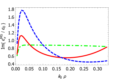
Let us begin with dependency on the size parameter $\rho$. In Fig. 2, the real and imaginary parts of $\varepsilon^{MG}_{x,y,z}/\varepsilon_{\scriptscriptstyle 0}$ are plotted against $k_{\scriptscriptstyle 0}\rho$, as computed using Eq. (8) with $U=3$, $\psi=50^{\circ}$, and $f_{a}=f_{b}=0.15$. Both real and imaginary parts of $\varepsilon^{MG}_{x,y,z,t}/\varepsilon_{\scriptscriptstyle 0}$ are acutely sensitive to $\rho$, for all free-space wavelengths considered. The plots for both the real and imaginary parts of $\varepsilon^{MG}_{x}/\varepsilon_{\scriptscriptstyle 0}$ and $\varepsilon^{MG}_{y}/\varepsilon_{\scriptscriptstyle 0}$ are qualitatively similar for all wavelengths considered. For $\lambda_{\scriptscriptstyle 0}\in\left\{600,750\right\}$ nm, the plots of $\mbox{Im}\left\{\varepsilon^{MG}_{x,y,z}/\varepsilon_{\scriptscriptstyle 0}\right\}$ exhibit a distinctive local maximum at small values of $\rho$ whereas the plots of $\mbox{Im}\left\{\varepsilon^{MG}_{t}/\varepsilon_{\scriptscriptstyle 0}\right\}$ exhibit a distinctive local minimum at small values of $\rho$. For $\lambda_{\scriptscriptstyle 0}\in\left\{600,750\right\}$ nm, the plots of $\mbox{Re}\left\{\varepsilon^{MG}_{x,y}/\varepsilon_{\scriptscriptstyle 0}\right\}$ exhibit a distinctive local minimum at small values of $\rho$ whereas the plots of $\mbox{Re}\left\{\varepsilon^{MG}_{t}/\varepsilon_{\scriptscriptstyle 0}\right\}$ exhibit a distinctive local maximum at small values of $\rho$. The real and imaginary parts of $\varepsilon^{MG}_{x,y,z,t}/\varepsilon_{\scriptscriptstyle 0}$ are highly sensitive to $k_{\scriptscriptstyle 0}\rho$ for the entire range of nanoparticle size considered, but in Fig. 1 we see that the permittivity of gold nanoparticles is highly sensitive to $\rho$ only for $\rho\lessapprox{\color[rgb]{0,0,1}25}$ nm. Therefore, the sensitivity exhibited in Fig. 2 for large values of $k_{\scriptscriptstyle 0}\rho$ is attributable to the size dependences of the depolarization dyadics $\underline{\underline{D}}_{\,U,c}$ and $\underline{\underline{D}}_{\,I,c}$ (as appropriate).

Figure 3: Real and imaginary parts of the non-zero components of the HCM’s relative permittivity dyadic versus orientation angle $\psi$ of gold nanoparticles for free-space wavelengths $\lambda_{\scriptscriptstyle 0}=450$ nm (green, broken dashed curve), 600 nm (red, solid curve), and 750 nm (blue, dashed curve). Size parameter $\rho=0.2/k_{\scriptscriptstyle 0}$, shape parameter $U=3$, and volume fractions $f_{a}=f_{b}=0.15$.

Next we turn to the dependency on inclusion orientation, as specified by the angle $\psi\in[0,\pi/2]$. The real and imaginary parts of $\varepsilon^{MG}_{x,y,z,t}/\varepsilon_{\scriptscriptstyle 0}$ are plotted against $\psi$ in Fig. 3 for $U=3$, $\rho=0.2/k_{\scriptscriptstyle 0}$, and $f_{a}=f_{b}=0.15$. Both real and imaginary parts of $\varepsilon^{MG}_{x,y,t}$ are acutely sensitive to $\psi$ but $\varepsilon^{MG}_{z}$ is independent of $\psi$, for all free-space wavelengths considered. Unlike $\varepsilon^{MG}_{x,y}$, $\varepsilon^{MG}_{t}$ is symmetric with respect to reflection about $\psi=\pi/4$ and is null valued for $\psi\in\left\{0,\pi/2\right\}$.

Figure 4: Real and imaginary parts of the non-zero components of the HCM’s relative permittivity dyadic versus shape parameter $U$ of gold nanoparticles for free-space wavelengths $\lambda_{\scriptscriptstyle 0}=450$ nm (green, broken dashed curve), 600 nm (red, solid curve), and 750 nm (blue, dashed curve). Size parameter $\rho=0.2/k_{\scriptscriptstyle 0}$, orientation angle $\psi=50^{\circ}$, and volume fractions $f_{a}=f_{b}=0.15$.

Now the inclusion shape is considered via the shape parameter $U\in(0,4]$. For $\rho=0.2/k_{\scriptscriptstyle 0}$, $\psi=50^{\circ}$, and $f_{a}=f_{b}=0.15$, the real and imaginary parts of $\varepsilon^{MG}_{x,y,z,t}/\varepsilon_{\scriptscriptstyle 0}$ are plotted against $U$ in Fig. 4. Both the real and imaginary parts of $\varepsilon^{MG}_{x,y,z,t}/\varepsilon_{\scriptscriptstyle 0}$ are acutely sensitive to $U$ for $\lambda_{\scriptscriptstyle 0}\in\left\{600,750\right\}$ nm but both are quite insensitive to $U$ for $\lambda_{\scriptscriptstyle 0}=450$ nm, for $U<3$. For $U>3$, $\varepsilon^{MG}_{x,y,z,t}/\varepsilon_{\scriptscriptstyle 0}$ is largely insensitive to $U$. Whereas the plots for $\varepsilon^{MG}_{x}/\varepsilon_{\scriptscriptstyle 0}$ and $\varepsilon^{MG}_{y}/\varepsilon_{\scriptscriptstyle 0}$ are qualitatively similar, those for $\varepsilon^{MG}_{z}/\varepsilon_{\scriptscriptstyle 0}$ and $\varepsilon^{MG}_{t}/\varepsilon_{\scriptscriptstyle 0}$ are somewhat different.

Figure 5: Real and imaginary parts of the non-zero components of the HCM’s relative permittivity dyadic versus volume fraction of gold for free-space wavelengths $\lambda_{\scriptscriptstyle 0}=450$ nm (green, broken dashed curve), 600 nm (red, solid curve), and 750 nm (blue, dashed curve). Size parameter $\rho=0.2/k_{\scriptscriptstyle 0}$, shape parameter $U=3$, orientation angle $\psi=50^{\circ}$, and volume fraction $f_{a}=0.3-f_{b}$.

The sensitivity of the HCM’s permittivity dyadic to the volume fraction of the inclusions is explored next. In Fig. 5, the real and imaginary parts of $\varepsilon^{MG}_{x,y,z,t}/\varepsilon_{\scriptscriptstyle 0}$ are plotted against $f_{b}$, with $\rho=0.2/k_{\scriptscriptstyle 0}$, $U=3$, $\psi=50^{\circ}$, and $f_{a}=0.3-f_{b}$. As in Figs. 2 and 4, the plots of both the real and imaginary parts of $\varepsilon^{MG}_{x}/\varepsilon_{\scriptscriptstyle 0}$ and $\varepsilon^{MG}_{y}/\varepsilon_{\scriptscriptstyle 0}$ in Fig. 5 are qualitatively similar for all wavelengths considered. The real parts of $\varepsilon^{MG}_{z}/\varepsilon_{\scriptscriptstyle 0}$ and $\varepsilon^{MG}_{t}/\varepsilon_{\scriptscriptstyle 0}$, as well as the imaginary part of $\varepsilon^{MG}_{z}/\varepsilon_{\scriptscriptstyle 0}$, increase uniformly as $f_{b}$ increases, whereas the imaginary part of $\varepsilon^{MG}_{t}/\varepsilon_{\scriptscriptstyle 0}$ does not, for all wavelengths considered.

The numerical results presented in Figs. 2–5 were computed using the extended Maxwell Garnett formalism, per Eq. (8), incorporating the size-dependent permittivity of gold nanoparticles delivered by Eqs. (2) and (3). Commonly, the unextended version of the Maxwell Garnett formalism [8] — which arises from the extended version in the limit $\rho\to 0$ — is implemented. It is also common for size-independent dielectric properties of the inclusion materials to be incorporated in the homogenization formalism used. Indeed, in a recent numerical study of gold-impregnated vaterite [9], a size-independent permittivity scalar was adopted for gold nanoparticles along with a non-rigorous version of the Maxwell Garnett formalism that fails to properly account for the uniaxial anisotropy of vaterite in the depolarization dyadics. In the case of spherical inclusions of air and gold (i.e., $U=1$), this non-rigorous formalism’s estimate of the HCM’s permittivity dyadic is given by

$$\underline{\underline{\tilde{\varepsilon}}}_{\,MG} = \underline{\underline{\varepsilon}}_{\,c}+\Bigg{\{}f_{a}\left(\varepsilon_{a}\underline{\underline{I}}-\underline{\underline{\varepsilon}}_{\,c}\right)$$ (11)

$$\mbox{ \tiny{${}^{\bullet}$} }\left[\underline{\underline{\varepsilon}}_{\,c}+\frac{1-f_{a}}{3}\left(\varepsilon_{a}\underline{\underline{I}}-\underline{\underline{\varepsilon}}_{\,c}\right)\right]^{-1}$$

$$+f_{b}\left(\varepsilon_{b}\underline{\underline{I}}-\underline{\underline{\varepsilon}}_{\,c}\right)$$

$$\mbox{ \tiny{${}^{\bullet}$} }\left[\underline{\underline{\varepsilon}}_{\,c}+\frac{1-f_{b}}{3}\left(\varepsilon_{b}\underline{\underline{I}}-\underline{\underline{\varepsilon}}_{\,c}\right)\right]^{-1}\Bigg{\}}\mbox{ \tiny{${}^{\bullet}$} }\underline{\underline{\varepsilon}}_{\,c}.$$

Figure 6: Real and imaginary parts of the non-zero components of the HCM’s relative permittivity dyadic versus relative size of gold nanoparticles. (a) Blue, dashed curves: estimates delivered by the extended Maxwell Garnett formalism, with size-dependent $\varepsilon_{b}$. (b) Green, broken-dashed curves: as (a) but computed using size-independent $\varepsilon_{b}=\left(-7.1698+i6.5253\right)\varepsilon_{\scriptscriptstyle 0}$. (c) Red, solid curves: as (a) but computed using unextended Maxwell Garnett formalism. (d) Black, solid horizontal lines: estimates delivered by the unextended Maxwell Garnett formalism, with size-independent $\varepsilon_{b}=\left(-7.1698+i6.5253\right)\varepsilon_{\scriptscriptstyle 0}$. (e) Black, dashed horizontal lines: estimates delivered by Eq. (11), with size-independent $\varepsilon_{b}=\left(-7.1698+i6.5253\right)\varepsilon_{\scriptscriptstyle 0}$. Free-space wavelength $\lambda_{\scriptscriptstyle 0}=600$ nm, shape parameter $U=1$, and volume fractions $f_{a}=f_{b}=0.15$.

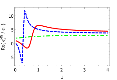
It is of interest to compare and contrast the estimate of $\underline{\underline{\varepsilon}}_{\,HCM}$ provided by the extended Maxwell Garnett formalism, incorporating the size-dependent permittivity of gold nanoparticles, with estimates provided by these related approaches in which the sizes of the inclusions and/or the anisotropy of vaterite are not taken into account. For this purpose, let us fix the free-space wavelength $\lambda_{\scriptscriptstyle 0}=600$ nm, shape parameter $U=1$ (in which case the orientation angle $\psi$ becomes irrelevant), and volume fractions $f_{a}=f_{b}=0.15$. Since the inclusions are spherical, the HCM’s permittivity dyadic has the uniaxial form

$$\underline{\underline{\varepsilon}}_{\,HCM}=\varepsilon^{HCM}_{x}\left(\hat{\underline{u}}_{\rm x}\,\hat{\underline{u}}_{\rm x}+\hat{\underline{u}}_{\rm y}\,\hat{\underline{u}}_{\rm y}\right)+\varepsilon^{HCM}_{z}\hat{\underline{u}}_{\rm z}\,\hat{\underline{u}}_{\rm z}.$$ (12)

In Fig. 6, the real and imaginary parts of $\varepsilon^{HCM}_{x}/\varepsilon_{\scriptscriptstyle 0}$ and $\varepsilon^{HCM}_{z}/\varepsilon_{\scriptscriptstyle 0}$ are plotted against $k_{\scriptscriptstyle 0}\rho$ using estimates from

• $\underline{\underline{\varepsilon}}^{MG}$ computed using Eq. (8) with a size-dependent $\varepsilon_{b}$ (blue, dashed curves);

• $\underline{\underline{\varepsilon}}^{MG}$ as computed in (a) but with size-independent $\varepsilon_{b}=\left(-7.1698+i6.5253\right)\varepsilon_{\scriptscriptstyle 0}$, which is the permittivity of gold nanoparticles of radius $\rho=3$ nm per Eqs. (2) and (3) (green, broken-dashed curves);

• $\underline{\underline{\varepsilon}}^{MG}$ as computed in (a) but with the unextended Maxwell Garnett formalism (red, solid curves);

• $\underline{\underline{\varepsilon}}^{MG}$ delivered by the unextended Maxwell Garnett formalism, with size-independent $\varepsilon_{b}=\left(-7.1698+i6.5253\right)\varepsilon_{\scriptscriptstyle 0}$ (black, solid horizontal lines); and

• $\underline{\underline{\tilde{\varepsilon}}}_{\,MG}$ delivered by Eq. (11), with size-independent $\varepsilon_{b}=\left(-7.1698+i6.5253\right)\varepsilon_{\scriptscriptstyle 0}$ (black, dashed horizontal lines).

All five estimates of the real and imaginary parts of $\varepsilon^{HCM}_{x}$ and $\varepsilon^{HCM}_{z}$ approximately agree at $\rho=3$ nm. For smaller values of $\rho$, the three estimates based on a size-independent $\varepsilon_{b}$, i.e., (a), (d), and (e), approximately agree, and the two estimates based on a size-dependent $\varepsilon_{b}$, i.e., (b) and (c), are in close agreement, but the estimates (b) and (c) differ markedly from the estimates (a), (d) and (e). For larger values of $\rho$, especially for $\rho>10$ nm, quite large differences emerge between the estimates (a), (b), and (c); however, the estimates (d) and (e) remain quite close to each other.

Finally in this section, let us consider again the issue of orientation of the inclusions. The results presented in Figs. 2–6 are based on the assumption that all inclusions have the same orientation, as specified by the dyadic $\underline{\underline{S}}(\gamma,\beta,\psi)$. We now assume that all orientations of inclusions in the $xy$ plane are equally likely. Accordingly, the dyadic $\underline{\underline{U}}$ introduced in Eq. (4) is replaced by its orientational average

$$\hat{\underline{\underline{U}}}=\frac{1}{2\pi}\int^{2\pi}_{0}\underline{\underline{U}}\,d\psi,$$ (13)

which yields

$$\hat{\underline{\underline{U}}}=\rho\sqrt[3]{\left(\frac{2}{U+1}\right)^{2}}\left[\frac{U+1}{2}\left(\hat{\underline{u}}_{\rm x}\,\hat{\underline{u}}_{\rm x}+\hat{\underline{u}}_{\rm y}\,\hat{\underline{u}}_{\rm y}\right)+\hat{\underline{u}}_{\rm z}\,\hat{\underline{u}}_{\rm z}\right].$$ (14)

Since the symmetry axis of $\hat{\underline{\underline{U}}}$ is parallel to the optic axis of the vaterite host material, the permittivity dyadic of the corresponding HCM has the uniaxial form given in Eq. (12). Now we repeat the computations of Fig. 2 but with $\underline{\underline{U}}$ replaced by its orientational average $\hat{\underline{\underline{U}}}$. The corresponding real and imaginary parts of the non-zero components of the HCM’s relative permittivity dyadic are plotted against relative size of gold nanoparticles in Fig. 7. The plots of both the real and imaginary parts of $\varepsilon^{MG}_{z}/\varepsilon_{\scriptscriptstyle 0}$ in Fig. 7 are very similar to those in Fig. 2 for all wavelengths considered. But the plots of the real and imaginary parts of $\varepsilon^{MG}_{x}/\varepsilon_{\scriptscriptstyle 0}$ in Fig. 7 are both quite different to those in Fig. 2; for example, the $\mbox{Re}\left\{\varepsilon^{MG}_{x}/\varepsilon_{\scriptscriptstyle 0}\right\}$ plot in Fig. 7 is concave whereas the corresponding plot in Fig. 2 is convex.

Parenthetically, homogenization formalisms such as the Maxwell Garnett and Bruggeman formalisms, as well as their extended variants, can accommodate other orientational statistics for $\underline{\underline{U}}$ in Eq. (4) than those considered here. Furthermore, $\underline{\underline{U}}$ can be different for inclusions made of different materials in these formalisms [8].

Figure 7: As Fig. 2 except that $\underline{\underline{U}}$ is replaced by its orientational average $\hat{\underline{\underline{U}}}$.

3 Closing remarks

The non-zero components of the permittivity dyadic of a biaxial dielectric HCM — constituted by porous vaterite impregnated with gold nanoparticles — have been estimated using the extended Maxwell Garnett formalism. The extended formalism takes into account the anisotropy of the vaterite as well as the size, shape, and orientation of the nanoparticles and pores; and a size-dependent permittivity was used for the gold nanoparticles. Numerical studies revealed that the HCM’s permittivity parameters are acutely sensitive to the size, shape, orientation, and volume fraction of the gold nanoparticles. Therefore, all of these attributes must be taken into account in theoretical studies of such HCMs. In particular, when the size of the gold nanoparticles is neglected, the Maxwell Garnett formalism can provide quite different estimates of the HCM’s permittivity parameters.

Lastly, surface roughness of nanoparticles may also have a significant bearing on the permittivity dyadic of impregnated vaterite [26]. However, as conventional approaches to homogenization such as the Maxwell Garnett formalism are based on convex-shaped inclusions, surface roughness cannot be accommodated by such conventional approaches. This remains a matter for future research.

Appendix

In order to specify the size-dependent depolarization dyadic $\underline{\underline{D}}_{\,U,c}$ given in the extended Maxwell Garnett formula (8), it is convenient to adopt the most general linear framework in which case the host material $c$ is a bianisotropic material, characterized by four 3$\times$3 constitutive dyadics in the Tellegen formalism: the permittivity dyadic $\underline{\underline{\varepsilon}}_{\,c}$, the permeability dyadic $\underline{\underline{\mu}}_{\,c}$, and two magnetoelectric dyadics $\underline{\underline{\xi}}_{\,c}$ and $\underline{\underline{\zeta}}_{\,c}$. In the case of vaterite, $\underline{\underline{\mu}}_{\,c}=\mu_{\scriptscriptstyle 0}\underline{\underline{I}}$ and $\underline{\underline{\xi}}_{\,c}=\underline{\underline{\zeta}}_{\,c}=\underline{\underline{0}}$.

The size-dependent 6$\times$6 depolarization dyadic of an inclusion embedded in a bianisotropic host material $c$ may be represented as the sum

$$\underline{\underline{\bf D}}_{\,U/\mbox{\tiny{c}}}=\underline{\underline{\bf D}}^{0}_{\,U/\mbox{\tiny{c}}}+\underline{\underline{\bf D}}^{+}_{\,U/\mbox{\tiny{c}}}.$$ (15)

Herein the size-independent contribution [11, 22]

$$\underline{\underline{\bf D}}^{0}_{\,U/\mbox{\tiny{c}}}=\frac{1}{4\pi}\int^{2\pi}_{\phi=0}\int^{\pi}_{\theta=0}\,\underline{\underline{\check{\bf G}}}^{\infty}_{\,\mbox{\tiny{c}}}(\underline{\underline{U}}^{-1}\mbox{ \tiny{${}^{\bullet}$} }\hat{\underline{q}})\sin\theta\,d\theta\,d\phi,$$ (16)

with the 6$\times$6 dyadic

$$\underline{\underline{\check{\bf G}}}^{\infty}_{\,\mbox{\tiny{c}}}(\underline{\underline{U}}^{-1}\mbox{ \tiny{${}^{\bullet}$} }\hat{\underline{q}})=\displaystyle{\frac{1}{i\omega\,b_{\,U/\mbox{\tiny{c}}}(\theta,\phi)}}\times$$

$$\left[\begin{array}[]{cc}\beta_{\mu}(\theta,\phi)\;\underline{\underline{U}}^{-1}\mbox{ \tiny{${}^{\bullet}$} }\hat{\underline{q}}\hat{\underline{q}}\mbox{ \tiny{${}^{\bullet}$} }\underline{\underline{U}}^{-1}&-\beta_{\xi}(\theta,\phi)\;\underline{\underline{U}}^{-1}\mbox{ \tiny{${}^{\bullet}$} }\hat{\underline{q}}\hat{\underline{q}}\mbox{ \tiny{${}^{\bullet}$} }\underline{\underline{U}}^{-1}\vspace{4pt}\\ -\beta_{\zeta}(\theta,\phi)\;\underline{\underline{U}}^{-1}\mbox{ \tiny{${}^{\bullet}$} }\hat{\underline{q}}\hat{\underline{q}}\mbox{ \tiny{${}^{\bullet}$} }\underline{\underline{U}}^{-1}&\beta_{\varepsilon}(\theta,\phi)\;\underline{\underline{U}}^{-1}\mbox{ \tiny{${}^{\bullet}$} }\hat{\underline{q}}\hat{\underline{q}}\mbox{ \tiny{${}^{\bullet}$} }\underline{\underline{U}}^{-1}\end{array}\right];$$ (19)

the scalar functions

$$\left.\begin{array}[]{l}\beta_{\sigma}(\theta,\phi)=\hat{\underline{q}}\mbox{ \tiny{${}^{\bullet}$} }\underline{\underline{U}}^{-1}\mbox{ \tiny{${}^{\bullet}$} }\underline{\underline{\sigma}}_{\,\mbox{\tiny{c}}}\mbox{ \tiny{${}^{\bullet}$} }\underline{\underline{U}}^{-1}\mbox{ \tiny{${}^{\bullet}$} }\hat{\underline{q}},\quad\left(\sigma\in\left\{\varepsilon,\xi,\zeta,\mu\right\}\right)\vspace{8pt}\\ b_{\,U/\mbox{\tiny{c}}}(\theta,\phi)=\left[\beta_{\varepsilon}(\theta,\phi)\,\beta_{\mu}(\theta,\phi)\right]-\left[\beta_{\xi}(\theta,\phi)\,\beta_{\zeta}(\theta,\phi)\right]\end{array}\right\};$$ (21)

and the unit vector

$$\hat{\underline{q}}=\frac{1}{q}\,\underline{q}=\sin\theta\cos\phi\,\hat{\underline{u}}_{\rm x}\,+\sin\theta\sin\phi\,\hat{\underline{u}}_{\rm y}\,+\cos\theta\,\hat{\underline{u}}_{\rm z}\,.$$ (22)

The size-dependent contribution is [23, 24]

$$\underline{\underline{\bf D}}^{+}_{\,U/\mbox{\tiny{c}}} = \frac{\omega^{4}}{4\pi}\int^{2\pi}_{\phi=0}\int^{\pi}_{\theta=0}\frac{1}{b_{\,U/\mbox{\tiny{c}}}(\theta,\phi)}\Bigg{[}\frac{1}{\kappa_{+}-\kappa_{-}}\Bigg{(}\frac{\exp\left(i\rho q\right)}{2q^{2}}$$ (23)

$$\times\left(1-i\rho q\right)\Big{\{}\,\mbox{det}\left[\underline{\underline{\check{\bf A}}}_{\,\mbox{\tiny{c}}}(\underline{\underline{U}}^{-1}\mbox{ \tiny{${}^{\bullet}$} }\underline{q})\right]\,\underline{\underline{\check{\bf G}}}^{+}_{\,\mbox{\tiny{c}}}(\underline{\underline{U}}^{-1}\mbox{ \tiny{${}^{\bullet}$} }\underline{q})$$

$$+\mbox{det}\left[\underline{\underline{\check{\bf A}}}_{\,\mbox{\tiny{c}}}(-\underline{\underline{U}}^{-1}\mbox{ \tiny{${}^{\bullet}$} }\underline{q})\right]\,\underline{\underline{\check{\bf G}}}^{+}_{\,\mbox{\tiny{c}}}(-\underline{\underline{U}}^{-1}\mbox{ \tiny{${}^{\bullet}$} }\underline{q})\Big{\}}\Bigg{)}^{q=\sqrt{\kappa_{+}}}_{q=\sqrt{\kappa_{-}}}$$

$$+\frac{\mbox{det}\left[\underline{\underline{\check{\bf A}}}_{\,\mbox{\tiny{c}}}(\underline{0})\right]}{\kappa_{+}\,\kappa_{-}}\,\underline{\underline{\check{\bf G}}}^{+}_{\,\mbox{\tiny{c}}}(\underline{0})\Bigg{]}\,\sin\theta\;d\theta\;d\phi,$$

with the 6$\times$6 dyadics

$$\left.\begin{array}[]{l}\displaystyle{\underline{\underline{\check{\bf A}}}_{\,\mbox{\tiny{c}}}(\underline{q})=\left[\begin{array}[]{cc}\underline{\underline{0}}&(\underline{q}/\omega)\times\underline{\underline{I}}\\ \vspace{-6pt}\hfil\\ -(\underline{q}/\omega)\times\underline{\underline{I}}&\underline{\underline{0}}\end{array}\right]+\left[\begin{array}[]{cc}\underline{\underline{\varepsilon}}_{\,c}&\underline{\underline{\xi}}_{\,c}\\ \underline{\underline{\zeta}}_{\,c}&\underline{\underline{\mu}}_{\,c}\end{array}\right]\vspace{8pt}}\\ \displaystyle{\underline{\underline{\check{\bf G}}}^{+}_{\,\mbox{\tiny{c}}}(\underline{q})=\frac{1}{i\omega}\,\underline{\underline{\check{\bf A}}}^{-1}_{\,\mbox{\tiny{c}}}(\underline{q})-\underline{\underline{\check{\bf G}}}^{\infty}_{\,\mbox{\tiny{c}}}(\underline{\underline{U}}^{-1}\mbox{ \tiny{${}^{\bullet}$} }\hat{\underline{q}})}\end{array}\right\}.$$ (24)

and $\kappa_{\pm}$ representing the roots of the quadratic (in $q^{2}$) equation $\mbox{det}\left[\underline{\underline{\check{\bf A}}}_{\,\mbox{\tiny{c}}}(\underline{\underline{U}}^{-1}\mbox{ \tiny{${}^{\bullet}$} }\underline{q})\right]=0$, i.e.,

$$\mbox{det}\left[\underline{\underline{\check{\bf A}}}_{\,\mbox{\tiny{c}}}(\underline{\underline{U}}^{-1}\mbox{ \tiny{${}^{\bullet}$} }\underline{q})\right]\propto\left(q^{2}-\kappa_{+}\right)\left(q^{2}-\kappa_{-}\right)=0.$$ (25)

Thus, the desired 3$\times$3 depolarization dyadic $\underline{\underline{D}}_{\,U,c}$ arises as

$$\underline{\underline{D}}_{\,U,c}=\left[\,\begin{array}[]{ccc}\left[\underline{\underline{\bf D}}_{\,U/\mbox{\tiny{c}}}\right]_{1,1}&\left[\underline{\underline{\bf D}}_{\,U/\mbox{\tiny{c}}}\right]_{1,2}&\left[\underline{\underline{\bf D}}_{\,U/\mbox{\tiny{c}}}\right]_{1,3}\vspace{4pt}\\ \left[\underline{\underline{\bf D}}_{\,U/\mbox{\tiny{c}}}\right]_{2,1}&\left[\underline{\underline{\bf D}}_{\,U/\mbox{\tiny{c}}}\right]_{2,2}&\left[\underline{\underline{\bf D}}_{\,U/\mbox{\tiny{c}}}\right]_{2,3}\vspace{4pt}\\ \left[\underline{\underline{\bf D}}_{\,U/\mbox{\tiny{c}}}\right]_{3,1}&\left[\underline{\underline{\bf D}}_{\,U/\mbox{\tiny{c}}}\right]_{3,2}&\left[\underline{\underline{\bf D}}_{\,U/\mbox{\tiny{c}}}\right]_{3,3}\end{array}\,\right].$$ (26)

In general, numerical methods are needed to evaluate the double integrals in Eqs. (16) and (23), but for biaxial dielectric host materials those integrals in Eqs. (16) may be expressed in terms of incomplete elliptic integrals of the first and second kind [25].

Acknowledgments. This work was supported in part by EPSRC (grant number EP/V046322/1) and US NSF (grant number DMS-2011996). AL thanks the Charles Godfrey Binder Endowment at The Pennsylvania State University for ongoing support of his research endeavors.

References

• [1] C. Rodriguez-Navarro, C. Jimenez-Lopez, A. Rodriguez-Navarro, M. T. Gonzalez-Muñoz, and M. Rodriguez-Gallego, “Bacterially mediated mineralization of vaterite,” Geochimica et Cosmochimica Acta, vol. 71, pp. 1197–1213, 2007.
• [2] B. C. Chakoumakos, B. M. Pracheil, R. S. Wood, A. Loeppky, G. Anderson, R. Koenigs, and R. Bruch, “Texture analysis of polycrystalline vaterite spherulites from Lake Sturgeon otoliths,” Sci. Rep., vol. 9, art. no. 7151, 2019.
• [3] S. Wu, C.-Y. Chiang, and W. Zhou, “Formation mechanism of CaCO3 spherulites in the myostracum layer of limpet shells,” Crystals, vol. 7, art. no. 319, 2017.
• [4] J. D. H. Donnay and G. Donnay, “Optical determination of water content in spherulitic vaterite,” Acta Cryst., vol. 22, pp. 312–314, 1967.
• [5] A. M. Ferreira, A. S. Vikulina, and D. Volodkina, “CaCO3 crystals as versatile carriers for controlled delivery of antimicrobials,” J. Controlled Release, vol. 328, pp. 470–489, 2020.
• [6] A. R. Rastinehad, H. Anastos, E. Wajswol, J. S. Winoker, J. P. Sfakianos, S. K. Doppalapudi, M. R. Carrick, C. J. Knauer, B. Taouli, S. C. Lewis, A. K. Tewari, J. A. Schwartz, S. E. Canfield, A. K. George, J. L. West, and N. J. Halas, “Gold nanoshell-localized photothermal ablation of prostate tumors in a clinical pilot device study,” Proc. Nat. Acad. Sci. USA, art. no. 201906929, 2019.
• [7] A. Biswas, A. T. Nagaraja, and M. J. McShane, “Fabrication of nanocapsule carriers from multilayer-coated vaterite calcium carbonate nanoparticles,” ACS Appl. Mater. Interfaces, vol. 6, pp. 21193–21201, 2014.
• [8] T. G. Mackay and A. Lakhtakia, Modern Analytical Electromagnetic Homogenization with Mathematica${}^{\mbox{\tiny{\textregistered}}}$, Second Edition. Bristol, UK, 2020.
• [9] R. E. Noskov, A. Machnev, I. I. Shishkin, M. V. Novoselova, A. V. Gayer, A. A. Ezhov, E. A. Shirshin, S. V. German, I. D. Rukhlenko, S. Fleming, B. N. Khlebtsov, D. A. Gorin, and P. Ginzburg, “Golden vaterite as a mesoscopic metamaterial for biophotonic applications,” Adv. Mater., vol. 33, art. no. 2008484, 2021.
• [10] T. G. Mackay, “On extended homogenization formalisms for nanocomposites,” J. Nanophoton., vol. 2, art. no. 021850, 2008.
• [11] B. Michel, “A Fourier space approach to the pointwise singularity of an anisotropic dielectric medium,” Int. J. Appl. Electromagn. Mech., vol. 8, pp. 219–227, 1997.
• [12] A. Derkachova, K. Kolwas, and I. Demchenko, “Dielectric function for gold in plasmonics applications: size dependence of plasmon resonance frequencies and damping rates for nanospheres,” Plasmonics, vol. 11, pp. 941–951, 2016.
• [13] H. C. Chen, Theory of Electromagnetic Waves. McGraw–Hill, New York, NY, USA, 1983.
• [14] T. G. Mackay and A. Lakhtakia, Electromagnetic Anisotropy and Bianisotropy, 2nd Edition. World Scientific, Singapore, 2019.
• [15] G. Strang, Introduction to Linear Algebra, 5th Edition. Wellesley, Cambridge, MA, USA, 2016.
• [16] A. Lakhtakia, P. D. Sunal, V. C. Venugopal, and E. Ertekin, “Homogenization and optical response properties of sculptured thin films,” Proc. SPIE, vol. 3790, pp. 77–83, 1999.
• [17] A. Lakhtakia and R. Messier, Sculptured Thin Films: Nanoengineered Morphology and Optics. SPIE, Bellingham, WA, USA, 2005.
• [18] A. Lakhtakia, “Size–dependent Maxwell–Garnett formula from an integral equation formalism,” Optik vol. 91, pp. 131–133, 1992.
• [19] M. T. Prinkey, A. Lakhtakia, and B. Shanker, “On the extended Maxwell–Garnett and the extended Bruggeman approaches for dielectric–in–dielectric composites,” Optik vol. 96, pp. 25–30, 1994.
• [20] J. G. Fikioris, “Electromagnetic field inside a current carrying region,” J. Math. Phys. vol. 6, pp. 1617–1620, 1965.
• [21] J. J. H. Wang, “A unified and consistent view of the singularities of the electric dyadic Green’s function in the source region,” IEEE Trans. Antennas Propagat. vol. 30, pp. 463–468, 1982.
• [22] B. Michel and W. S. Weiglhofer, “Pointwise singularity of dyadic Green function in a general bianisotropic medium,” Arch. Elektron. Übertrag., vol. 51, pp. 219–223, 1997. Corrections: vol. 52, p. 310, 1998.
• [23] T .G. Mackay, “Depolarization volume and correlation length in the homogenization of anisotropic dielectric composites,” Waves Random Media, vol. 14, pp. 485–498, 2004. Corrections: Waves Random Complex Media, vol. 16, p. 85, 2006.
• [24] J. Cui and T. G. Mackay, “Depolarization regions of nonzero volume in bianisotropic homogenized composites,” Waves Random Complex Media, vol. 17, pp. 269–281, 2007.
• [25] W. S. Weiglhofer, “Electromagnetic depolarization dyadics and elliptic integrals,” J. Phys. A: Math. Gen., vol. 31, pp. 7191–7196, 1998.
• [26] Y.-W. Lu, L.-Y. Li, and J.-F. Liu, “Influence of surface roughness on strong light-matter interaction of a quantum emitter-metallic nanoparticle system,” Sci. Rep., vol. 8, art. no. 7115, 2018.